Computing the Independence Polynomial:
from the Tree Threshold down to the Roots

Abstract

We study an algorithm for approximating the multivariate independence polynomial $Z(\mathbf{z})$, with negative and complex arguments. While the focus so far has been mostly on computing combinatorial polynomials restricted to the univariate positive setting (with seminal results for the independence polynomial by Weitz (2006) and Sly (2010)), the independence polynomial with negative or complex arguments has strong connections to combinatorics and to statistical physics. The independence polynomial with negative arguments, $Z(-\mathbf{p})$, determines the Shearer region, the maximal region of probabilities to which the Lovász Local Lemma (LLL) can be extended (Shearer 1985). In statistical physics, complex zeros of the independence polynomial relate to existence of phase transitions.

Our main result is a deterministic algorithm to compute approximately the independence polynomial in any root-free complex polydisc centered at the origin. More precisely, we can $(1+\epsilon)$-approximate the independence polynomial $Z(\mathbf{z})$ for an $n$-vertex graph of degree at most $d$, for any complex vector $\mathbf{z}$ such that $Z(\mathbf{z^{\prime}})\neq 0$ for $|z^{\prime}_{i}|\leq(1+\alpha)|z_{i}|$, in running time $(\frac{n}{\epsilon\alpha})^{O(\log(d)/\sqrt{\alpha})}$. Our result also extends to graphs of unbounded degree that have a bounded connective constant. Our algorithm is essentially the same as Weitz’s algorithm for positive parameters up to the tree uniqueness threshold. The core of the analysis is a novel multivariate form of the correlation decay technique, which can handle non-uniform complex parameters. In summary, we provide a unifying algorithm for all known regions where $Z(\mathbf{z})$ is approximately computable. In particular, in the univariate real setting our work implies that Weitz’s algorithm works in an interval between two critical points $(-\lambda^{\prime}_{c}(d),\lambda_{c}(d))$, and outside of this interval an approximation of $Z(\lambda)$ is known to be NP-hard.

As an application, we provide an algorithm to test membership in Shearer’s region within a multiplicative error of $1+\alpha$, in running time $(n/\alpha)^{O(\sqrt{n/\alpha}\log d)}$. We also give a deterministic algorithm for Shearer’s lemma (extending the LLL) with $n$ events on $m$ independent variables under slack $\alpha$, with running time $(nm/\alpha)^{O(\sqrt{m/\alpha}\log d)}$.

On the hardness side, we prove that evaluating $Z(\mathbf{z})$ at an arbitrary point in Shearer’s region, and testing membership in Shearer’s region, are $\#P$-hard problems. For Weitz’s correlation decay technique in the negative regime, we show that the $1/\sqrt{\alpha}$ dependence in the exponent is optimal.

1 Introduction

The independence polynomial is the generating function of independent sets of a graph. Formally, given a graph $G=(V,E)$, and a vector $\mathbf{x}=\left(x_{v}\right)_{v\in V}$ of vertex activities, it is the multi-linear polynomial

$$Z_{G}(\mathbf{x})=\sum_{I\text{ indep. in }G}\>\prod_{v\in I}x_{v}.$$

Aside from its natural importance in combinatorics as a generating function, the independence polynomial has also been studied extensively in statistical physics where it arises as the partition function of the hard core lattice gas, which has been used as a model of adsorption. In both settings, the partition function and its derivatives encode important properties of the model. For example, in the combinatorial setting, $Z_{G}$ encodes a weighted count of the independent sets, while the derivatives of $\log Z_{G}$ encode relevant average quantities, such as the mean size of an independent set. As such, much effort has gone into understanding the complexity of computing $Z_{G}$. The exact evaluation of the independence polynomial at non-trivial evaluation points turns out to be #P-hard [47]. As for approximate computation, the problem is well studied in the setting where the activities are positive and real valued. In this setting, the problem has served to highlight some of the tightest known connections between phase transitions and computational complexity: we will discuss this line of work in more detail below.

In this paper, we are concerned instead with the problem of approximately computing the independence polynomial at possibly negative and even complex valued vertex activities. The interest in studying partition functions at complex values of the activities originally comes from statistical mechanics, where there is a paradigm of studying phase transitions in terms of the analyticity of $\log Z_{G}$. This paradigm has led to the question of characterizing regions of the complex plane where the partition function is non-zero [49, 26]. Inspired by previous connections between statistical physics and computation complexity, a natural question is: does the maximum radius around the origin within which $\log Z_{G}$ is analytic (i.e., within which $Z_{G}$ has no roots) correspond to a transition in the computational complexity of computing $Z_{G}$? As we discuss below, the answer is yes.

A second motivation for studying the independence polynomial at complex activities comes from a delightful connection between combinatorics and statistical mechanics that arose in the work of Shearer [37] and Scott and Sokal [36] on the Lovász Local Lemma (LLL). In particular, the largest region of parameters in which the LLL applies is the maximal connected region of the negative orthant within which $Z_{G}$ has no roots. As we discuss below, an algorithm for approximating $Z_{G}$ at negative activities has several algorithmic applications relating to the LLL, including testing whether the hypotheses are satisfied, as well as giving a constructive proof of the LLL itself.

1.1 Our results

Before stating our results, let us define the Shearer region for graph $G$ to be

$$\mathcal{S}\leavevmode\nobreak\ =\leavevmode\nobreak\ \mathcal{S}_{G}\leavevmode\nobreak\ \,:=\,\leavevmode\nobreak\ \left\{\;\mathbf{p}\in[0,1]^{V}\,:\,Z_{G}\left(\mathbf{z}\right)\neq 0\leavevmode\nobreak\ \leavevmode\nobreak\ \forall\mathbf{z}\in\mathbb{C}^{V}\leavevmode\nobreak\ \text{s.t.}\leavevmode\nobreak\ \left|\mathbf{z}\right|\leq\mathbf{p}\;\right\},$$ (1.1)

which describes the radii of polydiscs within which $Z_{G}$ has no roots. Here, $\left|\mathbf{z}\right|$ means coordinate-wise magnitude, and $\leq$ also applies coordinate-wise. It can be shown that $\mathcal{S}_{G}$ is an open set.

Our main result is a fully polynomial time approximation scheme (FPTAS) for $Z_{G}(\mathbf{z})$ when $\mathbf{z}$ is a vector of possibly complex activities for which the vector $\left|\mathbf{z}\right|$ of their magnitudes lies in the Shearer region.

Theorem 1.1 (FPTAS for $Z_{G}$).

Let $G$ be an $n$-vertex graph with maximum degree $d$. Suppose that $\alpha,\epsilon\in(0,1]$, and that $\mathbf{z}\in\mathbb{C}^{V}$ satisfies $(1+\alpha)\cdot\left|\mathbf{z}\right|\in\mathcal{S}_{G}$. Then a $(1+\epsilon)$-approximation to $Z_{G}(\mathbf{z})$ can be computed in time $\big{(}\frac{n}{\epsilon\alpha}\big{)}^{O(\log(d)/\sqrt{\alpha})}$.

As the set $\mathcal{S}_{G}$ is somewhat mysterious, it is instructive to consider the following univariate corollary.

Figure 1: Summary of results for computation of $Z_{G}(z\mathbf{1})$ in the complex univariate setting, as a function of the degree $d$. Here $\lambda^{\prime}_{c}=\frac{(d-1)^{d-1}}{d^{d}}\searrow\frac{1}{ed}$ and $\lambda_{c}=\frac{(d-1)^{d-1}}{(d-2)^{d}}\searrow\frac{e}{d}$. Note that a major difference of this work from Patel-Regts [33] that is not captured by this figure is that our running time has a significantly better dependence on distance from the boundary of Shearer’s region, which is crucial in our applications.

Corollary 1.2 (FPTAS for the univariate case).

Let $G$ be an $n$-vertex graph with maximum degree $d$. Define $\lambda_{G}=\min\{\,\left|z\right|\,:\,z\in\mathbb{C},\,Z_{G}(z\mathbf{1})=0\,\}$. Let $\alpha,\epsilon\in(0,1]$ and $z\in\mathbb{C}$ satisfy $(1+\alpha)\left|z\right|\leq\lambda_{G}$. Then a $(1+\epsilon)$-approximation to $Z_{G}(z\mathbf{1})$ can be deterministically computed in time $\big{(}\frac{n}{\epsilon\alpha}\big{)}^{O((1/\sqrt{\alpha})\cdot\log(d))}$.

Remark: Region of applicability.

In order to understand $\lambda_{G}$ it is helpful to consider a bound that depends only on the degree $d$. Define $\lambda^{\prime}_{c}(d)$ to be the minimum of $\lambda_{G}$ over all graphs of maximum degree $d$. Then it is known [37] that $\lambda^{\prime}_{c}(1)=1/2$ and $\lambda^{\prime}_{c}(d)=\frac{(d-1)^{d-1}}{d^{d}}$ for $d\geq 2$; the minimum is achieved by the infinite $d$-regular tree. So $\lambda^{\prime}_{c}(d)$ is the threshold, depending only on $d$, that determines the region of applicability of our algorithm. This is no accident: approximating $Z_{G}(z\mathbf{1})$ for real $z<-\lambda^{\prime}_{c}$ has recently been shown to be NP-hard by Galanis, Goldberg and Štefankovič [16], showing that Corollary 1.2 has the tightest possible range of applicability on the negative real line (i.e., the Shearer region). Thus, a phase transition in the computational complexity of the problem occurs right at the boundary of the region within which $Z_{G}$ is guaranteed to have no roots. As Figure 1 shows, we now have a complete picture of the computational complexity of $Z_{G}$ in the real univariate case, as a function of $d$.

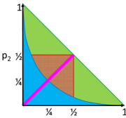
Figure 2: For illustrative purposes, let us consider the graph $G=K_{2}$; here $d=1$ and $\lambda^{\prime}_{c}(d)=1/2$. Our algorithm applies throughout Shearer’s region $\mathcal{S}_{G}$, shown as the green triangular region. The pink line segment is the restriction of $\mathcal{S}_{G}$ for the univariate function $Z_{G}(z\mathbf{1})$. The work of Patel-Regts describes an algorithm focused on the univariate case, but they mention [33, pp. 13] that it can be generalized to all points dominated by $\lambda^{\prime}_{c}$ (the red square region). The blue region, defined as $\mathcal{L}$ in Appendix A, is where the original LLL [14, 43] applies.

Remark: Dependence on Slack.

An important feature of Theorem 1.1 is that although the running time degrades as the input vector $\mathbf{p}$ approaches the boundary of the Shearer region $\mathcal{S}$, the degradation is only sub-exponential in $\frac{1}{\alpha}$ (being exponential in $\frac{1}{\sqrt{\alpha}}$) where $\alpha$ is the slack parameter that measures the distance to the boundary. This is in contrast to an earlier manuscript of the present paper [21] and the concurrent paper of Patel and Regts [33], which (using different methods), obtained an FPTAS whose running time is actually exponential in $\frac{1}{\alpha}$. We describe the new ideas required to get this better dependence on $\alpha$ in Section 3.2, and remark on the barriers to improving this dependence towards the end of this subsection.

The importance of a sub-exponential dependence on the slack is that for some applications it is imperative to approximate the independence polynomial at points that are extremely close to the boundary of the Shearer region and have slack at most $\Theta(1/n)$. We present two such applications here, for both of which we are able to obtain sub-exponential time algorithms, and for both of which the earlier results [21, 33] only give exponential time algorithms.

Remark: Connective constant.

Theorem 1.1 extends to graphs of unbounded maximum degree that have a bounded connective constant [30, 19, 39, 40]. See Appendix F for the details of this extension.

Application 1: Testing membership in Shearer region.

Physicists have studied the univariate threshold $\lambda_{G}$ for specific graphs, as this determines the region within which there are no phase transitions [49]. For example, to understand phase transitions in $\mathbb{Z}^{2}$, researchers have performed numerical computations on finite graphs to estimate the exact value $\lambda_{G}(\mathbb{Z}^{2})$. (See, e.g., [24] [36, Section 8.4] [46].) Computations have shown that $\lambda_{G}(\mathbb{Z}^{2})\leq 1/8$ (rigorous) and $\lambda_{G}(\mathbb{Z}^{2})=0.119,338,881,88(1)$ (non-rigorous).

Our first application is an algorithm to test whether a given vector $\mathbf{p}$ lies in the Shearer region, up to accuracy $\alpha$. This can be used to compute bounds on $\lambda_{G}$, and could potentially be useful for physicists.

Theorem 1.3.

Given a graph $G$, $\mathbf{p}\in(0,1)^{V}$, and $\alpha\in(0,1]$, there exists a deterministic algorithm which, in running time $(n/\alpha)^{O(\sqrt{n/\alpha}\log d)}$ decides whether $\mathbf{p}\in{\cal S}_{G}$ or $(1+\alpha)\mathbf{p}\notin{\cal S}_{G}$.

This algorithm uses the FPTAS of Theorem 1.1 in a black box fashion, calling it at points in $\mathcal{S}$ that may have slack $O(1/n)$. Replacing the black box by an algorithm that had an exponential dependence on the slack would give an algorithm with only a trivial exponential time guarantee on its run-time. We note also that the testing membership in $\mathcal{S}$ is #P-hard when $\alpha$ is exponentially small. (See Appendix E for a precise statement of this hardness result.)

Application 2: Constructive algorithm for the Lovász Local Lemma by polynomial evaluation.

The LLL is a tool in combinatorics giving conditions ensuring that it is possible to avoid certain bad events $\mathcal{E}_{1},\ldots,\mathcal{E}_{n}$. (For readers unfamiliar with the LLL, a statement is provided in Appendix A.) Although the LLL guarantees that there exists a point in $\bigcap_{i=1}^{n}\overline{\mathcal{E}_{i}}$, it provides no hint on how to find such a point. For decades, algorithmically constructing such a point was a major research challenge, though over the past 10 years dramatic progress has been made. Any such algorithm must necessarily make some assumptions on the probability space, the most common being the “variable model” used by [31]. All previous algorithms have been based on the idea of randomly sampling variables followed by brute-force search [8, 2], or random resampling [44, 32, 31, 25, 1, 20, 22], or derandomizations of those ideas [8, 2, 32, 31, 10].

We develop a completely new algorithmic approach to the LLL in the variable model. The previous randomized algorithms can be viewed as generating a sequence of infeasible, integral solutions; at each step, they resample one of the bad events and hopefully move closer to feasibility. (The previous deterministic algorithms are derandomizations of this approach.) In contrast, our new algorithm generates a sequence of feasible, fractional solutions; at each step, it fixes the value of one of the variables while preserving feasibility in $\mathcal{S}_{G}$. The value of the polynomial $Z_{G}(\mathbf{z})$ is used to determine membership in $\mathcal{S}_{G}$. Thus, our algorithm can be viewed as a rounding algorithm for the LLL, and the value of $Z_{G}(\mathbf{z})$ can be viewed as a pessimistic estimator for the probability of $\bigcap_{i=1}^{n}\overline{\mathcal{E}_{i}}$. To compute $Z_{G}(\mathbf{z})$, our algorithm uses (as a black box) our deterministic FPTAS for evaluating the independence polynomial with negative activities and slack $\Omega(1/m)$, where $m$ is the number of variables.

Theorem 1.4.

Consider an LLL scenario in the variable model (as in Section A.1): $\mu_{\mathbf{z}}$ is the product distribution on $\left\{0,1\right\}^{m}$ with expectation $\mathbf{z}$, $G$ is the dependency graph for events $\mathcal{E}_{1},\ldots,\mathcal{E}_{n}$, and $p_{i}=\mu_{\mathbf{z}}(\mathcal{E}_{i})$. There is a deterministic algorithm that takes as input a description of the events $\mathcal{E}_{1},\ldots,\mathcal{E}_{n}$, a vector $\mathbf{z}\in[0,1]^{m}$, and a parameter $\alpha\in(0,1]$ such that $(1+\alpha)\cdot\mathbf{p}(\mathbf{z})\in\mathcal{S}_{G}$. The algorithm runs for time $(nm/\alpha)^{O(\log(d)\sqrt{m/\alpha})}$ and outputs a point in $\bigcap_{i=1}^{n}\overline{\mathcal{E}_{i}}$.

This algorithm uses our FPTAS from Theorem 1.1 as a black box. Note that our algorithm runs in subexponential time, so, as of now, its runtime is not competitive with the state of the art deterministic algorithms for the LLL [10]. Nevertheless, prior to our work there was essentially only one known algorithmic technique known for the LLL: the witness tree technique originating with Beck [8]. Our work provides the only other known technique that gives an algorithm for the LLL better than brute-force. The fact that our algorithm is slow is only because the best known implementation of the black box (i.e., Theorem 1.1) has a running time that depends sub-exponentially on the slack. The algorithm thus points to a new intriguing connection between approximate counting and algorithmic versions of the LLL, and suggests the open question of finding the optimal dependence on the slack $\sqrt{\alpha}$ in Theorem 1.1.

Dependence on the “slack parameter” $\alpha$.

The discussion following the two applications above suggests that the question of the optimal dependence on the slack $\alpha$ in Theorem 1.1 is of importance for further exploration of the connection between approximate counting and the LLL. While we cannot yet provide a complete answer to this question, we conclude this section with a couple of our results that address this point. Our first result in this direction shows that some dependence on the slack parameter is inevitable. (See Section E.2 for a proof).

Theorem 1.5 (Necessity of slack).

If there is an algorithm to estimate $Z_{G}(-\mathbf{p})$, assuming $(1+\alpha)\mathbf{p}\in\mathcal{S}$, within a $\mathop{\mathrm{poly}}\left(n\right)$ multiplicative factor in running time $(n\log\frac{1}{\alpha})^{O(\log n)}$ then $\text{\#P}\subseteq\text{DTIME}(n^{O(\log n)})$.

However, this hardness result, while applying to all algorithmic approaches, only provides a weak lower bound on what can be achieved. We do not yet have any stronger general lower bounds, but our second result, described in detail in Appendix G, presents evidence that the dependence on $1/\sqrt{\alpha}$ in Theorem 1.1 is optimal for the techniques used in our paper. Nevertheless, it does not preclude the possibility that other approximate counting techniques could substantially improve upon Theorem 1.1. We discuss some related future directions in Section 6.

1.2 Related work

As discussed above, the exact computation of the independence polynomial turns out to be #P-hard. This is a fate shared by the partition functions of several other “spin systems” (e.g., the Ising model) in statistical physics, and by now there is extensive work on the complexity theoretic classification of partition functions in terms of dichotomy theorems (see e.g., [9]).

The approximation problem for a univariate partition function with a positive real argument is also well studied and has strong connections with phase transitions in statistical mechanics. In two seminal papers, Weitz [48] and Sly [41] (see also [42, 15, 17]) showed that there exists a critical value $\lambda_{c}(d)$ such when $\lambda<\lambda_{c}(d)$, there is an FPTAS for the partition function $Z_{G}(\lambda)$ on graphs of maximum degree $d$, while for $\lambda>\lambda_{c}(d)$ close to the threshold, approximating $Z_{G}(\lambda)$ on $d$-regular graphs is NP-hard under randomized reductions. (Sly and Sun [42] extended the hardness result to any $\lambda>\lambda_{c}(d)$.)

The approach for our FPTAS builds upon the correlation decay technique pioneered by Weitz, which has since inspired several results in approximate counting (see, e.g., [27, 18, 13, 28, 39, 29, 38, 7]). Unlike previous work, where the partition function has positive activities and induces a probability distribution on the underlying structures, our emphasis is on negative and complex activities. It turns out that Weitz’s proof can be easily modified to handle a univariate independence polynomial with a negative (and indeed, complex) parameter $z$ satisfying $\left|z\right|<\lambda^{\prime}_{c}(d)=\frac{(d-1)^{d-1}}{d^{d}}$, analogous to the $\lambda<\lambda_{c}(d)$ condition mentioned above; this observation appears in [45]. Our work considers a much more general scenario: the multivariate independence polynomial under a global condition incorporating all vertex activities (i.e., the set $\mathcal{S}$). This yields a result for the univariate case stronger than [45], as our threshold $\lambda_{G}$ in Corollary 1.2 depends on $G$ not just on $d$.

Starting with a paper of Barvinok [4], a different approach to approximating partition functions in their zero-free regions has emerged. Here, the analyticity of $\log Z$ in the zero-free region of $Z$ is used to provide an additive approximation to $\log Z$ (which translates to a multiplicative approximation for $Z$) via a Taylor expansion truncated at an appropriate degree. While this method has by now been applied to several classes of partition functions [3, 5, 6, 34], the resulting algorithms had turned out to be quasi-polynomial in the earlier applications because of the lack of a method to efficiently compute coefficients of terms of degree $\Omega(\log n)$ in the Taylor expansion of $\log Z$ (which, in the case of the hard core model, correspond to $\Omega(\log n)$-wise correlations among vertices in a random independent set). In work that was circulated concurrently with an earlier manuscript [21] of this paper, Patel and Regts [33] showed that for a class of models, these coefficients could be computed in polynomial time on bounded degree graphs, and as a consequence obtained an FPTAS for some partition functions in the region of analyticity of their logarithms. This included the univariate independence polynomial in bounded-degree graphs of degree $d$ when the activity $\lambda$ satisfies $\left|\lambda\right|<\lambda^{\prime}_{c}$. While their particular result for the univariate independence polynomial seems to be implied by the observations in [45] pointed out above, their technique applies also to other models. We note however that the present work has advantages over the result of Patel and Regts in two qualitative aspects which are both crucial for our applications.

First, as mentioned above, the running time of our FPTAS is sub-exponential in $1/\alpha$ when the input activity (or more generally, the input probability vector in the multivariate case) has slack $\alpha$, whereas their algorithm has an exponential dependence on $1/\alpha$. Indeed, it appears that this exponential dependence on $1/\alpha$ is intrinsic to their approach since the rate of convergence of the power series they use for approximating $\log Z$ is exactly $1-\alpha$ for an activity that has slack $\alpha$, so that the number of terms of the series that need to be evaluated for an additive $\epsilon/n$-approximation to $\log Z$ (which corresponds to a $(1\pm\Theta(\epsilon/n))$ multiplicative approximation for $Z$) is $\Omega(\log_{1/(1-\alpha)}\log(n/\epsilon))=\Omega\left(\frac{\log(n/\epsilon)}{\alpha}\right)$. Since the complexity of computing the $k$th term of this series in their framework is $\Omega(d^{k})$, this leads to a run time that is $\left(\nicefrac{{n}}{{\epsilon}}\right)^{\Omega\left((1/\alpha)\cdot\log(d)\right)}$ (our algorithm, in contrast will run in time $\left(\nicefrac{{n}}{{\alpha\epsilon}}\right)^{O\left((1/\sqrt{\alpha})\cdot\log(d)\right)}$). As discussed above, this improvement over Patel and Regts [33] is crucial for the applications considered in this paper. Second, our paper explicitly handles the multivariate independence polynomial. The work of Patel-Regts describes an algorithm focused on the univariate case, but they mention [33, pp. 13] that it can be generalized to all points dominated by $\lambda^{\prime}_{c}$ (the red square region in Figure 2). Though it seems plausible that their method can be extended to be applicable throughout the Shearer region (albeit still with an exponential dependence on the slack $\alpha$), to the best of our knowledge, the algorithmic details for doing so have not yet been published.

1.3 Techniques

As in previous work, our starting point is the standard self-reducibility argument showing that the problem of designing an FPTAS for $Z_{G}(\lambda)$ is equivalent to the problem of designing an FPTAS for computing the occupation ratio $r_{v}$ of a given vertex $v$ in any given graph $G$ (i.e., the ratio of the total weights of the independent sets containing $v$ to the total weight of those that do not). In previous work, these occupation ratios are actual likelihood ratios that can be translated to the probability that the vertex $v$ is occupied, but because of complex weights, we do not have the luxury of this interpretation. However, as in earlier work, we can still write formal recurrences for these occupation ratios. As Weitz showed [48], this recursive computation is naturally structured as a tree which has the same structure as the the tree $T_{\mathrm{SAW}}(v,G)$ whose nodes correspond to self-avoiding walks in $G$ starting at $v$. However the tree $T_{\mathrm{SAW}}(v,G)$ has size exponential in $|V|$, so this reduction does not immediately give a polynomial time algorithm.

The crucial step in correlation decay algorithms is to show that this tree can be truncated to polynomial size without incurring a large error in the value computed at the root. In earlier work on positive activities, especially since Restrepo et al. [35], the standard method for doing this has been to consider instead a recurrence for an appropriately chosen function $\phi(r_{v})$, known as the message, that is chosen so that when correlation decay holds on the $d$-regular tree, each step of the recurrence on the truncated $T_{\mathrm{SAW}}$ contracts the error introduced by the truncation by a constant factor. Thus, by expanding the tree to $\ell=O(\log\frac{n}{\epsilon})$ levels (so $d^{\ell}=\mathop{\mathrm{poly}}\left(n,\frac{1}{\epsilon}\right)$ nodes), one obtains a $(1+O(\frac{\epsilon}{n}))$-approximation to the value at the root.

Our approach also involves truncating the computation tree at an appropriate depth and then controlling the errors introduced due to truncation. However, in part because of the lack of a uniform bound on the vertex activities, we are not able to recreate a message-based approach. Instead, we perform a direct amortization argument, where we define recursively for each node in the computation tree an error sensitivity parameter, and then measure errors at that node as a fraction of the local error sensitivity parameter. We then establish two facts: (1) that the errors, when measured as a fraction of the error sensitivity parameter, do indeed decay by a constant fraction (roughly $(1-\Omega(\sqrt{\alpha}))$ when the input probability vector has slack $\alpha$) at each step of the recurrence (even though the absolute errors may not), and (2) that the error sensitivity parameter of the root node is not too large, so that the absolute error of the final answer can be appropriately bounded. The detailed argument appears in Section 3.2. For readers familiar with the earlier manuscript [21] of this paper, we point out that in that manuscript, the decay at each step of the recurrence could only be shown to be of the form $(1-O(\alpha))$; informal and formal descriptions of how this is improved to $(1-\Omega(\sqrt{\alpha}))$ in the present paper also appear in Section 3.2.

2 Overview of the correlation decay method

In this section we summarize the basic concepts and facts relating to Weitz’s correlation decay method. Since all the claims are simple or known, the proofs are omitted or appear in the appendix.

Partition functions and occupation ratios.

Since we are primarily interested in the hard-core partition function (i.e., independence polynomial) with negative activities, it will be convenient to introduce the following notation. Let $G=(V,E)$ be a fixed graph, and let $\mathbf{p}$ be a fixed vector of (possibly complex) parameters on the vertices of $V$. For $S\subseteq V$, let $\operatorname{Ind}(S)=\operatorname{Ind}_{G}(S)=\left\{\;I\subseteq S\,:\,I\text{ independent in }G\;\right\}$. Following the notation of [25, 23], we define the alternating-sign independence polynomial for any subset $S$ of $V$ to be

$$\breve{q}_{S}\>=\>\breve{q}_{S}(\mathbf{p})\,:=\,\sum_{\begin{subarray}{c}I\in\operatorname{Ind}(S)\end{subarray}}(-1)^{\left|I\right|}\prod_{v\in I}p_{v}.$$

Note that $\breve{q}_{V}(\mathbf{p})=Z_{G}(-\mathbf{p})$. The computation of $\breve{q}_{V}$ will be reduced to the computation of occupation ratios defined as follows. For a pair $(S,u)$, where $S\subseteq V$ and $u\in S$, the occupation ratio $r_{S,u}$ is

$$r_{S,u}=r_{S,u}(\mathbf{p})\,:=\,-\frac{\sum_{I\in\operatorname{Ind}(S),u\in I}(-1)^{|I|}\prod_{v\in I}p_{v}}{\sum_{I\in\operatorname{Ind}(S),u\notin I}(-1)^{|I|}\prod_{v\in I}p_{v}}.$$ (2.1)

For readers familiar with the notation of Weitz [48], we note that $r_{S,u}$ agrees with his definition of occupation ratios except for the negative signs used in the definition here. Using the definition of $\breve{q}_{S}$, and the notation $\Gamma(u)=\left\{\;v\,:\,u\text{ is a neighbor of }v\text{ in }G\;\right\}$, $\Gamma^{+}(u)=\Gamma(u)\cup\left\{u\right\}$, we can also rewrite this quantity as

$$r_{S,u}=\frac{p_{u}\breve{q}_{S\setminus\Gamma^{+}(u)}}{\breve{q}_{S\setminus\left\{u\right\}}}=-\frac{\breve{q}_{S}-\breve{q}_{S\setminus\left\{u\right\}}}{\breve{q}_{S\setminus\left\{u\right\}}}=1-\frac{\breve{q}_{S}}{\breve{q}_{S\setminus\left\{u\right\}}}.$$ (2.2)

A standard self-reducibility argument now reduces the computation of $\breve{q}_{V}$ to that of the $r_{S,u}$.

Claim 2.1.

Fix an arbitrary ordering $(v_{1},v_{2},\dots,v_{n})$ of $V$, and let $S_{i}=\left\{v_{i},v_{i+1},\dots,v_{n}\right\}$. We then have

$$\breve{q}_{V}=\prod_{i=1}^{n}\frac{\breve{q}_{S_{i}}}{\breve{q}_{S_{i+1}}}=\prod_{i=1}^{n}(1-r_{S_{i},v_{i}}).$$ (2.3)

Recurrences for the occupation ratios.

An important observation in Weitz’s work [48] was that the computation of occupation ratios similar to the $r_{S,u}$ can be carried out over a tree-like recursive structure. We follow a similar strategy, although we find it convenient to work with a somewhat different notation.

Definition 2.2 (Child subproblems).

Given a pair $(S,u)$ with $S\subseteq V$ and $u\in S$, and an arbitrary ordering $(v_{1},v_{2},\dots,v_{k})$ of $\Gamma(u)\cap S$, we define the set of child sub-problems $\mathcal{C}(S,u)=\mathcal{C}_{(v_{1},v_{2},\dots,v_{k})}(S,u)$ to be

$$\mathcal{C}(S,u)\leavevmode\nobreak\ =\leavevmode\nobreak\ \left\{\,(S\setminus\left\{u\right\},v_{1}),\,(S\setminus\left\{u,v_{1}\right\},v_{2}),\,\dots,\,(S\setminus\left\{u,v_{1},\ldots,v_{k-1}\right\},v_{k})\right\}.$$

Note that the ordering of neighbors used in the definition of $\mathcal{C}(S,u)$ is completely arbitrary and orderings between neighbors of different vertices do not share any consistency constraints. The recurrence relation for the computation of the $r_{S,u}$, analogous to Weitz’s computation tree, is then the following:

Lemma 2.3 (Computational recurrence).

Fix a graph $G=(V,E)$ and a vector $\mathbf{p}\in\mathbb{C}^{V}$ of complex parameters. Let $(S,u)$ be such that $u\in S$ and $S\subseteq V$. Fix an arbitrary ordering $(v_{1},v_{2},\dots,v_{k})$ of $\Gamma(u)\cap S$ and define the corresponding set $\mathcal{C}(S,u)$ of child subproblems. We then have

$$r_{S,u}=p_{u}\cdot\prod_{(S^{\prime},u^{\prime})\in\mathcal{C}(S,u)}\frac{1}{1-r_{S^{\prime},u^{\prime}}}.$$ (2.4)

Remark 2.1.

As observed by Weitz [48], each node in the computation tree of $r_{V,v}$ at depth $\ell$ corresponds to a unique self-avoiding walk of length $\ell$ starting at $v$.

The Shearer region.

The Shearer region was defined (implicitly) by Shearer [37] as follows.

Definition 2.4 (Shearer region and slack).

Given a graph $G=(V,E)$, the Shearer region $\mathcal{S}$ is the set of vectors $\mathbf{p}\in(0,1)^{V}$ such that $\breve{q}_{S}(\mathbf{p})>0$ for all $S\subseteq V$. A probability vector $\mathbf{p}$ is said to have slack $\alpha\geq 0$ if the vector $(1+\alpha)\mathbf{p}$ is also a probability vector and is contained in $\mathcal{S}$.

Shearer proved that this is the maximal region of probability vectors to which the LLL can be extended. The equivalence with our earlier definition (1.1) is due to Scott and Sokal [36, Theorem 2.10]: the Shearer region can be equivalently defined by the absence of roots in a certain polydisc, as follows.

Theorem 2.5.

A probability vector $\mathbf{p}\in(0,1)^{V}$ is in the Shearer region (as defined in Definition 2.4) if and only if for all vectors $\mathbf{z}=\left(z_{v}\right)_{v\in V}$ of complex activities such that $\left|z_{v}\right|\leq p_{v}$, it holds that $Z_{G}(\mathbf{z})\neq 0$.

Considering this, it is natural to extend the definition of the Shearer region to complex parameters. In the following, we consider primarily this complex extension of the Shearer region.

Definition 2.6 (Complex Shearer region).

Given a graph $G=(V,E)$, the complex Shearer region is

$$\mathcal{S}\,=\,\mathcal{S}_{G}\,:=\,\left\{\;\mathbf{p}\in\mathbb{C}^{V}\,:\,Z_{G}(\mathbf{z})\neq 0\leavevmode\nobreak\ \>\forall\mathbf{z}\in\mathbb{C}^{V},\,|z_{v}|\leq|p_{v}|\;\right\}.$$

We now state some important properties of the occupation ratios and $\breve{q}_{S}$ in the setting of real, positive parameters $\mathbf{p}$. These results are essentially translations of the results of [37, 36] into our notation.

Lemma 2.7 (Monotonicity and positivity of $\breve{q}$).

Let $G=(V,E)$ be any graph and let $\mathbf{p}\in(0,1)^{V}$ be such that $\mathbf{p}\in\mathcal{S}$. Then for any subsets $A$ and $B$ of $V$ such that $A\subseteq B$, we have $\breve{q}_{A}(\mathbf{p})\geq\breve{q}_{B}(\mathbf{p})>0$.

Lemma 2.8 (Occupation ratios are bounded).

Let $G=(V,E)$ be any graph and let $\mathbf{p}\in(0,1)^{V}$ be such that $\mathbf{p}\in\mathcal{S}$. Then, for any subset $S$ of $V$ and any vertex $u\in S$, we have $p_{u}\leq r_{S,u}<1$.

The correlation decay algorithm.

Weitz’s high-level approach to compute the independence polynomial is to compute the partition function via a telescoping product analogous to (2.3), and to compute each occupation ratio via a recurrence analogous to (2.4). As discussed in Section 1.3, the recursion is truncated to $\ell$ levels, and the analysis shows that the occupation ratio at the root is not affected heavily by the occupation ratios where the truncation occurred.

We follow that same high-level approach here, although the details of the analysis are quite different. Algorithm 1 presents pseudocode giving a compact description of the full algorithm. The main procedure, ComputeIndependencePolynomial($G,\mathbf{p},\ell$) implements (2.3) to estimate $\breve{q}_{V}(\mathbf{p})$ for a graph $G=(V,E)$, a parameter vector $\mathbf{p}$, and a desired recursion depth $\ell$. (The required value of $\ell$ depends upon the the accuracy parameter $\epsilon$; see Theorem 3.9). The recursive procedure OccupationRatio($G,\mathbf{p},\ell,S,u$) implements (2.4) to estimate the occupation ratio $r_{S,u}$ by executing $\ell$ levels of recursion.

Algorithm 1 Our algorithm to compute a $(1+\epsilon)$-approximation to $\breve{q}_{V}(\mathbf{p})$.

1:procedure ComputeIndependencePolynomial($G=(V,E),\mathbf{p},\ell$)

2:     Fix an ordering $V=(v_{1},v_{2},\ldots,v_{n})$

3:     $\breve{q}\leftarrow 1$

4:     for $i\leftarrow 1,\ldots,n$ do

5:         $\breve{q}\leftarrow\breve{q}\cdot(1-\text{\sc OccupationRatio}(G,\mathbf{p},\ell,\{v_{i},\ldots,v_{n}\},v_{i}))$      

6:     return $\breve{q}$

7:procedure OccupationRatio($G,\mathbf{p},\ell,S,u$)

8:     if $\ell=0$ then return $0$

9:     Let $(w_{1},w_{2},\ldots,w_{k})$ denote a fixed ordering of $S\cap\Gamma(u)$

10:     $r\leftarrow p_{u}$

11:     for $i\leftarrow 1,\ldots,k$ do

12:         $r\leftarrow r/(1-\text{\sc OccupationRatio}(G,\mathbf{p},\ell-1,S\setminus\{u,w_{1},\ldots,w_{i-1}\},w_{i}))$      

13:     return $r$

3 The analysis

Let us turn to the analysis of the correlation decay method in our setting. The notion of correlation decay in the hard core model refers to the decaying dependence of the occupation probability at a given vertex $v$ on the conditioning on a set of vertices at a certain distance from $v$. In the setting of positive activities $\mathbf{z}$ [48], these correlations are closely tied to the decay of errors in the computation tree for $r_{S,u}$ described in (2.4). For negative or general complex activities, the occupation ratios $r_{S,u}$ do not have a direct interpretation in terms of occupation probabilities. However, the analysis of errors in the computation tree is reminiscent of that of [48] and hence we still refer to it as correlation decay.

Unlike Weitz’s setting [48], where all vertex activities are the same, and the bounds are derived uniformly for all graphs with degrees bounded by $d$, here we are aiming for a more refined analysis for a particular graph $G$ and a (possibly non-uniform) vector $\mathbf{p}$. In Weitz’s setting, the worst-case errors in the recursive tree can be proved to decay in a uniform fashion (possibly after an application of an appropriate potential function or message). That is not the case here, since the local structure of $G$ and $\mathbf{p}$ might cause the errors to locally increase, even if the computation eventually converges. Hence it is critical to identify a local sensitivity parameter that describes how the errors propagate in the recursive tree.

3.1 The error sensitivity parameter

For simplicity of notation, we fix the input graph $G=(V,E)$ and an ordering on vertices $V=\{v_{1},\ldots,v_{n}\}$ for the rest of this section. Recall that $\mathbf{p}=(p_{1},p_{2},\dots,p_{n})$ denotes a vector of vertex parameters in the complex plane. (We have $\mathbf{p}=-\mathbf{z}$ where $\mathbf{z}$ are the usual activities in the hard core model.) We use $\left|\mathbf{p}\right|$ to denote the vector $(\left|p_{1}\right|,\left|p_{2}\right|,\dots,\left|p_{n}\right|)$. Note that $\mathbf{p}$ is in the Shearer region $\mathcal{S}$ if and only if $\left|\mathbf{p}\right|$ is in $\mathcal{S}$.

First, let us consider how the errors propagate throughout the recursive computation in Algorithm 1. Let $R_{S,u}$ an estimate obtained by the algorithm for the occupation ratio $r_{S,u}=1-\breve{q}_{S}/\breve{q}_{S\setminus\{u\}}$. We are interested in how the additive approximation error $|r_{S,u}-R_{S,u}|$ propagates in the recursive computation.

It turns out that $\mathbf{p}$ being real positive is in some sense the worst case; to simplify notation, we define for $u\in S$ and $\mathbf{p}\in\mathbb{C}^{V}$,

$$\varrho_{S,u}(\mathbf{p})\,:=\,r_{S,u}(\left|\mathbf{p}\right|).$$

The reader who wishes to understand the main ideas while avoiding some mild technical details may henceforth assume that $\mathbf{p}$ is a real positive vector, and therefore $\varrho_{S,u}(\mathbf{p})=r_{S,u}(\mathbf{p})$. Indeed, an easy recursive argument shows that when $\mathbf{p}\in\mathcal{S}$, $\varrho_{S,u}(\mathbf{p})$ dominates both $r_{S,u}(\mathbf{p})$ and $R_{S,u}(\mathbf{p})$ (see 3.6):

$$\left|r_{S,u}(\mathbf{p})\right|\leq\varrho_{S,u}(\mathbf{p})\text{ and }\left|R_{S,u}(\mathbf{p})\right|\leq\varrho_{S,u}(\mathbf{p}).$$

Now, from the mean value theorem, we obtain the following recursive bound.

Claim 3.1.

Let $\mathbf{p}$ lie in the complex Shearer region. For a node $(S,u)$ with children $\mathcal{C}(S,u)$ in the recursive computation tree, we have

$$\left|r_{S,u}-R_{S,u}\right|\leq\varrho_{S,u}\sum_{c\in\mathcal{C}(S,u)}\frac{\left|r_{c}-R_{c}\right|}{1-\varrho_{c}}.$$ (3.1)

Proof.

Recall Lemma 2.3, $r_{S,u}=p_{u}\prod_{c\in\mathcal{C}(S,u)}\frac{1}{1-r_{c}}$. Using the mean value theorem (Theorem C.3) with $\gamma_{c}\,:=\,\varrho_{c}$, we obtain

$$\left|r_{S,u}-R_{S,u}\right|\leq\left|p_{u}\right|\prod_{c\in\mathcal{C}(S,u)}\frac{1}{1-\varrho_{c}}\sum_{c^{\prime}\in\mathcal{C}(S,u)}\frac{\left|r_{c^{\prime}}-R_{c^{\prime}}\right|}{1-\varrho_{c^{\prime}}}=\varrho_{S,u}\sum_{c\in\mathcal{C}(S,u)}\frac{\left|r_{c}-R_{c}\right|}{1-\varrho_{c}}.$$

Note that the conditions imposed in the hypothesis of Theorem C.3 hold, since, as pointed out above, $\left|r_{S,u}\right|,\left|R_{S,u}\right|\leq\varrho_{S,u}$ for all nodes $(S,u)$ in the computation tree (see 3.6). ∎

Our error sensitivity parameter is defined to capture how errors propagate under this recursive bound. An important observation is that the derivative of $\varrho_{S,u}((1+t)\mathbf{p})$ with respect to $t$ satisfies a recurrence very similar to Claim 3.1, and this is the main motivation behind the following definition.

Definition 3.2 (Error sensitivity parameter).

The error sensitivity parameter $\beta_{S,u}\,:=\,\beta_{S,u}(\mathbf{p})$ is defined as

$$\beta_{S,u}(\mathbf{p})\,:=\,\left.\frac{\text{d}\varrho_{S,u}((1+t)\mathbf{p})}{\text{d}t}\right|_{t=0}.$$ (3.2)

Claim 3.3.

Let $(S,u)$ be node in the computation tree. Then

$$\beta_{S,u}=\varrho_{S,u}\cdot\left(1+\sum_{c\in\mathcal{C}(S,u)}\frac{\beta_{c}}{1-\varrho_{c}}\right).$$

Proof.

By a direct calculation using the definition of $\beta_{S,u}$,

$$\beta_{S,u}\,:=\,\frac{\text{d}\varrho_{S,u}((1+t)\mathbf{p})}{\text{d}t}\Big{|}_{t=0}=\frac{\text{d}}{\text{d}t}\Bigg{(}(1+t)\left|p_{u}\right|\cdot\prod_{c\in\mathcal{C}(S,u)}\frac{1}{1-\varrho_{c}((1+t)\mathbf{p})}\Bigg{)}\Bigg{|}_{t=0}$$

$$\>=\prod_{c\in\mathcal{C}(S,u)}\frac{1}{1-\varrho_{c}(\mathbf{p})}\cdot\Bigg{(}\left|p_{u}\right|+\Big{(}(1+t)\left|p_{u}\right|\Big{)}\cdot\!\!\sum_{c\in\mathcal{C}(S,u)}\frac{1}{1-\varrho_{c}((1+t)\mathbf{p})}\cdot\frac{\text{d}\varrho_{c}((1+t)\mathbf{p})}{\text{d}t}\Bigg{)}\Bigg{|}_{t=0}$$

$$\>=\prod_{c\in\mathcal{C}(S,u)}\frac{1}{1-\varrho_{c}(\mathbf{p})}\cdot\Big{(}\left|p_{u}\right|+\left|p_{u}\right|\sum_{c\in\mathcal{C}(S,u)}\frac{\beta_{c}}{1-\varrho_{c}}\Big{)}$$

$$\>=\varrho_{S,u}(\mathbf{p})\cdot\Big{(}1+\sum_{c\in\mathcal{C}(S,u)}\frac{\beta_{c}}{1-\varrho_{c}}\Big{)}.\qed$$

We will now prove several additional properties of the error sensitivity parameter.

Lemma 3.4.

Fix a parameter vector $\mathbf{p}\in\mathcal{S}$. Let $t_{0}$ be such that for $0\leq t\leq t_{0}$, $(1+t)\mathbf{p}$ is also in $\mathcal{S}$. Define $\beta_{S,u}(\mathbf{p},t)=\frac{\text{d}}{\text{d}t}\varrho_{S,u}((1+t)\mathbf{p})$. (Note that Definition 3.2 is consistent with $\beta_{S,u}(\mathbf{p})=\beta_{S,u}(\mathbf{p},0)$.) Then, for all nodes $(S,u)$ in the computation tree, $\beta_{S,u}(\mathbf{p},t)$ is a non-negative, non-decreasing function of $t$ for $t\in[0,t_{0}]$. Thus, the map $t\mapsto\varrho_{S,u}((1+t)\mathbf{p})$ is non-decreasing and convex over the same domain.

Proof.

We induct on $|S|$. The base case is $S=\left\{u\right\}$, so $\varrho_{\{u\},u}((1+t)\mathbf{p})=(1+t)\left|p_{u}\right|$. We therefore have

$$\beta_{\{u\},u}(\mathbf{p},t)=\frac{\text{d}}{\text{d}t}\varrho_{\{u\},u}((1+t)\mathbf{p})=|p_{u}|,$$

which is a constant (and hence non-decreasing), non-negative function of $t$.

For the inductive case, we use a recursive formula for $\beta_{S,u}(p,t)$ as in the proof of 3.3. We have

$$\beta_{S,u}(\mathbf{p},t)={\left|p_{u}\right|\cdot\prod_{(S^{\prime},u^{\prime})\in\mathcal{C}(S,u)}\frac{1}{1-\varrho_{S^{\prime},u^{\prime}}((1+t)\mathbf{p})}\>+\>\varrho_{S,u}((1+t)\mathbf{p})\cdot\sum_{(S^{\prime},u^{\prime})\in\mathcal{C}(S,u)}\frac{\beta_{S^{\prime},u^{\prime}}(\mathbf{p},t)}{1-\varrho_{S^{\prime},u^{\prime}}((1+t)\mathbf{p})}}.$$

By the induction hypothesis, $\beta_{S^{\prime},u^{\prime}}(\mathbf{p},t)\geq 0$ for each $|S^{\prime}|<|S|$, $u^{\prime}\in S^{\prime}$. Since $(1+t)\mathbf{p}\in\mathcal{S}$, Lemma 2.8 implies $0\leq\varrho_{S^{\prime},u^{\prime}}((1+t)\mathbf{p})<1$. Therefore $\beta_{S,u}(\mathbf{p},t)\geq 0$ as well. Moreover, the inductive hypothesis implies that both $\varrho_{S^{\prime},u^{\prime}}((1+t)\mathbf{p})$ and $\beta_{S^{\prime},u^{\prime}}(\mathbf{p},t)$ are non-decreasing in $t$. Since the whole expression is monotone in $\varrho_{S^{\prime},u^{\prime}}$ and $\beta_{S^{\prime},u^{\prime}}(\mathbf{p},t)$, the left-hand side $\beta_{S,u}(\mathbf{p},t)$ is also a non-decreasing function of $t$. ∎

We can now prove the following relations between the $\beta_{S,u}$ and the $\varrho_{S,u}$.

Lemma 3.5.

Let $\mathbf{p}\in\mathbb{C}^{V}$ and $\alpha>0$ satisfy $(1+\alpha)\mathbf{p}\in\mathcal{S}$. We then have the following inequalities for all nodes $(S,u)$ in the computation tree. (We use the shorthand notation $\varrho_{S,u}=\varrho_{S,u}(\mathbf{p})$ and $\beta_{S,u}=\beta_{S,u}(\mathbf{p})$.)

1. $\beta_{S,u}<(1-\varrho_{S,u})/\alpha$.

2. $\varrho_{S,u}\leq\beta_{S,u}\leq(1+d_{u}/\alpha)\cdot\varrho_{S,u}$, where $d_{u}$ is the degree of the vertex $u$ in $G$.

3. $\varrho_{S,u}\leq\frac{1}{1+\alpha}\varrho_{S,u}((1+\alpha)\mathbf{p})<\frac{1}{1+\alpha}$.

Proof.

Since $(1+\alpha)\mathbf{p}\in\mathcal{S}$, Lemma 2.8 implies $\varrho_{S,u}((1+\alpha)\mathbf{p})<1$. Further, from Lemma 3.4, we know that $t\mapsto\varrho_{S,u}((1+t)\mathbf{p})$ is convex for $t\in[0,\alpha]$. Item 1 of the lemma then follows from the inequalities

$$1\leavevmode\nobreak\ >\leavevmode\nobreak\ \varrho_{S,u}((1+\alpha)\mathbf{p})\leavevmode\nobreak\ \geq\leavevmode\nobreak\ \varrho_{S,u}+\alpha\frac{\text{d}\varrho_{S,u}}{\text{d}t}\Big{|}_{t=0}\leavevmode\nobreak\ \geq\leavevmode\nobreak\ \varrho_{S,u}+\alpha\beta_{S,u}.$$ (3.3)

Item 2 follows from 3.3, using $\beta_{S,u}\geq 0$, $\left|\mathcal{C}(S,u)\right|\leq d_{u}$, and $\beta_{S,u}<(1-\varrho_{S,u})/\alpha$ from item 1.

To prove the first inequality in item 3, we again use eq. 3.3, and substitute $\beta_{S,u}\geq\varrho_{S,u}$ from item 2. The second inequality follows from the fact that $\varrho_{S,u}((1+\alpha)\mathbf{p})<1$ as mentioned above. ∎

Finally we relate the quantities $\varrho_{S,u}$ to the quantities $r_{S,u}$ that we actually want to approximate.

Claim 3.6.

Let $\mathbf{p}$ lie in the complex Shearer region. For any node $(S,u)$ in the computation tree, we have

$$\left|r_{S,u}(\mathbf{p})\right|\leq\varrho_{S,u}(\mathbf{p})\text{ and }\left|R_{S,u}(\mathbf{p})\right|\leq\varrho_{S,u}(\mathbf{p}).\vspace*{-4pt}$$

Proof.

For both $r_{S,u}$ and $R_{S,u}$, the proof is by induction on $|S|$. The base case for $r_{S,u}$ is when $S$ is a singleton, in which case we have $\left|r_{\left\{u\right\},u}(\mathbf{p})\right|=\left|p_{u}\right|=\varrho_{\left\{u\right\},u}(\mathbf{p})$. For $R_{S,u}$, the base case is when $(S,u)$ is at depth $\ell$ in the computation tree (where $\ell$ is as in the input to Algorithm 1), in which case one has $R_{S,u}(\mathbf{p})=0\leq\rho_{S,u}(\mathbf{p})$. For the inductive case, we use the recursion for $r_{S,u}(\mathbf{p})$ to obtain

$$\left|r_{S,u}(\mathbf{p})\right|=\left|p_{u}\prod_{c\in\mathcal{C}(S,u)}\frac{1}{1-r_{c}(\mathbf{p})}\right|\leq\left|p_{u}\right|\prod_{c\in\mathcal{C}(S,u)}\frac{1}{1-\left|r_{c}(\mathbf{p})\right|}\leq\left|p_{u}\right|\prod_{c\in\mathcal{C}(S,u)}\frac{1}{1-\varrho_{c}(\mathbf{p})}=\varrho_{S,u}.$$

Here, the first inequality follows from C.1 since the induction hypothesis implies that $\mathbf{p}\in\mathcal{S}$ $\left|r_{c}(\mathbf{p})\right|\leq\varrho_{c}(\mathbf{p})$, while that fact that $\mathbf{p}\in\mathcal{S}$ implies that $\varrho_{c}(\mathbf{p})<1$ (e.g., from item 3 of Lemma 3.5). The second inequality follows directly from the induction hypothesis. The inductive step for $R_{S,u}$ is identical. ∎

3.2 Correlation decay with complex activities

We now use the error sensitivity parameters to establish the correlation decay results needed for our FPTAS.

Let $G=(V,E)$ be a graph on $n$ vertices, and let $\mathbf{p}\in\mathbb{C}^{V}$ be such that $(1+\alpha)^{2}\mathbf{p}\in\mathcal{S}$ ($\mathbf{p}$ is in the Shearer region with slack $\simeq 2\alpha$). The root of the recursion is a pair $(A,a)$ where $A\subseteq V$ and $a\in A$. Let $\ell\geq 0$ be arbitrary. Recall that Algorithm 1 recursively computes an estimate $R_{S,u}$ of $r_{S,u}$, where for every pair $(S,u)$ encountered, we have

$$R_{S,u}\leavevmode\nobreak\ =\leavevmode\nobreak\ \begin{cases}0&\quad\text{(if $(S,u)$ is at depth $\ell$ in the computation tree)}\\ p_{u}\cdot\prod_{c\in\mathcal{C}(S,u)}(1-R_{c})^{-1}&\quad\text{(otherwise)}\end{cases}.$$

The depth $\delta$ of a node is defined as its distance from the root $(A,a)$ in the recursive tree: the root has $\delta(A,a)=0$, its children have $\delta(S,u)=1$, etc.

Intuition.

2.1 implies that it is sufficient to get good approximations for the occupation ratios in order to obtain an FPTAS. Suppose now that we were to expand the computation tree for computing a particular occupation ratio up to depth $\ell$ as described above, and were then able to show that at every node $(S,u)$ in this tree, the approximation error $|r_{S,u}-R_{S,u}|$ is smaller than the maximum approximation error at the node’s children by a factor $c<1$. It would then follow that the approximation error at the root node is $O(c^{\ell})$, and hence that it is sufficient to take $\ell=O(\log n)$ in order to obtain an inverse polynomial approximation of the occupation ratio (which in turn can be shown to be sufficient for obtaining an FPTAS for $Z$). However, since degrees and the activity parameters might vary throughout the tree, the errors $|r_{S,u}-R_{S,u}|$ do not decay uniformly in this fashion at each node of the tree; they might even increase locally. (Examples are not difficult to construct.) Instead, we aim to use the error sensitivity parameter $\beta_{S,u}$ as a yardstick against which the approximation error $|r_{S,u}-R_{S,u}|$ at node $(S,u)$ ought to be compared.

As we mentioned earlier, $\beta_{S,u}$ is a natural error sensitivity parameter because it satisfies a recurrence (Claim 3.3) similar to the recurrence for error propagation (Claim 3.1). In an earlier version of this paper, we used “normalized errors” roughly of the form $|r_{S,u}-R_{S,u}|/\beta_{S,u}$, and showed that they decay by a factor of $1-\Theta(\alpha)$ at each level of the tree. Here we present an improved analysis which leads to a decay factor of $1-\Theta(\sqrt{\alpha})$, which is in fact tight (in particular on the infinite $d$-regular tree, see Appendix G).

The improvement comes from analyzing in conjunction the behavior of $r_{S,u}$ at two different probability vectors: $\mathbf{p}$ and the vector $(1+\alpha)\mathbf{p}$ of slightly larger probabilities (which nonetheless still has a slack of $\alpha$). We denote $\beta^{\prime}_{S,u}=\frac{d\varrho_{S,u}((1+t)\mathbf{p})}{dt}\Big{|}_{t=\alpha}$. Instead of $\beta_{S,u}$, we compare the errors to the quantity $\sqrt{\beta_{S,u}\beta^{\prime}_{S,u}}$, i.e., we normalize the error at node $(S,u)$ as $|r_{S,u}-R_{S,u}|/\sqrt{\beta_{S,u}\beta^{\prime}_{S,u}}$.

The reason for this choice of the normalization is as follows. It can be shown that the case where the earlier version of the normalized error decays by a factor of only $1-O(\alpha)$ corresponds to the situation where $\varrho_{S,u}((1+\alpha)\mathbf{p})\simeq(1+\alpha)\varrho_{S,u}(\mathbf{p})$. But in that case, an argument based on Lemmas 3.4 and 3.5 implies that $\beta_{S,u}-\varrho_{S,u}$ must be quite small. The new normalization of the error allows us to exploit this phenomenon: we can now show, roughly speaking, that the smaller of these two factors, i.e., $\varrho_{S,u}(\mathbf{p})/\varrho_{S,u}((1+\alpha)\mathbf{p})$ (which was the factor obtained in the analysis of the earlier version) on the one hand, and $\beta_{S,u}-\varrho_{S,u}$ on the other, can be taken to be the decay factor for the new normalized error. We then show that at least one of these two factors is as small as $1-\Omega(\sqrt{\alpha})$. At a technical level, proving this requires a careful comparison of the recurrences for the propagation of unnormalized errors (Claim 3.1) with the recurrence for the $\beta_{S,u}$ (Claim 3.3), exploiting in particular the extra additive term of $1$ in the latter recurrence. We now make this intuition precise in the following theorem. Recall that $\mathbf{p}$ is assumed to be such that $(1+\alpha)^{2}\mathbf{p}\in\mathcal{S}$.

Theorem 3.7.

For notational simplicity, let $\varrho_{S,v}=\varrho_{S,v}(\mathbf{p})$ and $\varrho^{\prime}_{S,v}=\varrho_{S,v}((1+\alpha)\mathbf{p})$. Similarly, let $\beta_{S,v}=\beta_{S,v}(\mathbf{p})$ and $\beta^{\prime}_{S,v}=\beta_{S,v}((1+\alpha)\mathbf{p})$. For a node $(S,u)$ in a computation tree of depth $\ell$,

$$\left|r_{S,u}-R_{S,u}\right|\leq\sqrt{\beta_{S,u}\beta^{\prime}_{S,u}}{(1+\sqrt{\alpha})^{-(\ell-0pt(S,u))/2}}.$$

Proof.

The proof is by induction on $\ell-0pt(S,u)$. The base case is $0pt(S,u)=\ell$ and $R_{S,u}=0$; we want to prove $|r_{S,u}|\leq\sqrt{\beta_{S,u}\beta^{\prime}_{S,u}}$. We have $\left|r_{S,u}\right|\leq\varrho_{S,u}$ (3.6). The base case follows since $\varrho_{S,u}\leq\beta_{S,u}$ and $\varrho_{S,u}\leq\varrho^{\prime}_{S,u}\leq\beta^{\prime}_{S,u}$, by Lemma 3.4, and item 2 of Lemma 3.5.

For the inductive step, we apply the recursive formula from Claim 3.1:

$$\left|r_{S,u}-R_{S,u}\right|\leq\varrho_{S,u}\sum_{c\in\mathcal{C}(S,u)}\frac{\left|r_{c}-R_{c}\right|}{1-\varrho_{c}}.$$

By definition, $0pt(c)=0pt(S,u)+1$ for all $c\in\mathcal{C}(S,u)$. By the induction hypothesis, we therefore have

$$\left|r_{S,u}-R_{S,u}\right| \leq\varrho_{S,u}\sum_{c\in\mathcal{C}(S,u)}\frac{\sqrt{\beta_{c}\beta^{\prime}_{c}}}{1-\varrho_{c}}(1+\sqrt{\alpha})^{-(\ell-0pt(S,u)-1)/2}$$

$$\leq\varrho_{S,u}\sum_{c\in\mathcal{C}(S,u)}\sqrt{\frac{\beta_{c}}{1-\varrho_{c}}}\cdot\sqrt{\frac{\beta^{\prime}_{c}}{1-\varrho^{\prime}_{c}}}\ (1+\sqrt{\alpha})^{-(\ell-0pt(S,u)-1)/2},$$

$$\leq\varrho_{S,u}\sqrt{\sum_{c\in\mathcal{C}(S,u)}\frac{\beta_{c}}{1-\varrho_{c}}}\cdot\sqrt{\sum_{c\in\mathcal{C}(S,u)}\frac{\beta_{c}^{\prime}}{1-\varrho^{\prime}_{c}}}\ (1+\sqrt{\alpha})^{-(\ell-0pt(S,u)-1)/2}$$

$$=\sqrt{\frac{\varrho_{S,u}}{\varrho^{\prime}_{S,u}}}\sqrt{\beta_{S,u}-\varrho_{S,u}}\cdot\sqrt{\beta_{S,u}^{\prime}-\varrho^{\prime}_{S,u}}(1+\sqrt{\alpha})^{-(\ell-0pt(S,u)-1)/2}$$ (3.4)

where the second inequality uses $\varrho_{c}\leq\varrho^{\prime}_{c}$ (which follows from item 3 of Lemma 3.5), the third is the Cauchy-Schwarz inequality, and the last equality uses the recursion for $\beta_{S,u}$ as developed in 3.3. Note that it also follows from items 2 and 3 of Lemma 3.5 that

$$0\leq\varrho_{S,u}\leq\varrho^{\prime}_{S,u}\text{ and }\beta_{S,u}-\varrho_{S,u},\beta^{\prime}_{S,u}-\varrho^{\prime}_{S,u}\geq 0.$$ (3.5)

We now divide the rest of the analysis into two cases.

Case 1: $\beta_{S,u}\leq\varrho_{S,u}/\sqrt{\alpha}$

. In this case, we have $0\leq\beta_{S,u}-\varrho_{S,u}\leq\beta_{S,u}(1-\sqrt{\alpha})\leq\beta_{S,u}/(1+\sqrt{\alpha})$. Substituting this into eq. 3.4, and estimating the rest of the factors using (3.5), we get

$$\left|r_{S,u}-R_{S,u}\right| \leq\sqrt{\frac{\varrho_{S,u}}{\varrho^{\prime}_{S,u}}}\sqrt{\beta_{S,u}-\varrho_{S,u}}\cdot\sqrt{\beta_{S,u}^{\prime}-\varrho^{\prime}_{S,u}}\ (1+\sqrt{\alpha})^{-(\ell-0pt(S,u)-1)/2}$$

$$\leq\sqrt{\beta_{S,u}\beta_{S,u}^{\prime}}\cdot\frac{1}{\sqrt{1+\sqrt{\alpha}}}\ (1+\sqrt{\alpha})^{-(\ell-0pt(S,u)-1)/2},$$

which completes the inductive step in this case.

Case 2: $\beta_{S,u}>\varrho_{S,u}/\sqrt{\alpha}$

. We claim that in this case, $\varrho_{S,u}\leq\varrho^{\prime}_{S,u}/(1+\sqrt{\alpha})$. Indeed, using the same argument as in the proof of item 1 of 3.3, we have

$$\varrho^{\prime}_{S,u}\leavevmode\nobreak\ \,:=\,\leavevmode\nobreak\ \varrho_{S,u}((1+\alpha)\mathbf{p})\leavevmode\nobreak\ \geq\leavevmode\nobreak\ \varrho_{S,u}+\alpha\frac{\text{d}\varrho_{S,u}}{\text{d}t}\Big{|}_{t=0}\leavevmode\nobreak\ \geq\leavevmode\nobreak\ \varrho_{S,u}+\alpha\beta_{S,u}\leavevmode\nobreak\ >\leavevmode\nobreak\ (1+\sqrt{\alpha})\varrho_{S,u}.$$ (3.6)

Substituting this into eq. 3.4, we obtain

$$\left|r_{S,u}-R_{S,u}\right| \leq\sqrt{\frac{\varrho_{S,u}}{\varrho^{\prime}_{S,u}}}\sqrt{\beta_{S,u}-\varrho_{S,u}}\cdot\sqrt{\beta_{S,u}^{\prime}-\varrho^{\prime}_{S,u}}\ (1+\sqrt{\alpha})^{-(\ell-0pt(S,u)-1)/2}$$

$$\leq\frac{1}{\sqrt{1+\sqrt{\alpha}}}\sqrt{\beta_{S,u}\beta_{S,u}^{\prime}}\ (1+\sqrt{\alpha})^{-(\ell-0pt(S,u)-1)/2},$$

which establishes the induction step in this case as well.∎

Corollary 3.8.

Given a graph $G=(V,E)$, let $\mathbf{p}$ be a complex parameter vector such that $(1+\alpha)^{2}\mathbf{p}\in\mathcal{S}$. Let $(A,a)$ be the root of the recursive computation of Theorem 3.7, where $a$ is a vertex of degree $d_{a}$ in $G$. Then, we have

$$\left|r_{A,a}-R_{A,a}\right|\leq\frac{1+d_{a}/\alpha}{(1+\sqrt{\alpha})^{\ell/2}}.$$

Proof.

Recall from Lemma 2.8 that $\varrho_{A,a}\in[0,1)$ when $\mathbf{p}\in\mathcal{S}$. Then item 2 of Lemma 3.5 implies that

$$\beta_{A,a}\big{(}(1+\alpha)\mathbf{p}\big{)}\leavevmode\nobreak\ \leq\leavevmode\nobreak\ (1+d_{a}/\alpha)\cdot r_{A,a}\big{(}(1+\alpha)\mathbf{p}\big{)}\leavevmode\nobreak\ \leq\leavevmode\nobreak\ 1+d_{a}/\alpha.$$

We can apply Lemma 3.5 to $\beta_{A,a}((1+\alpha)\mathbf{p})$ (as opposed to $\beta_{A,a}(\mathbf{p})$) because of the assumption that $(1+\alpha)^{2}\mathbf{p}\in S$. The claim now follows from Theorem 3.7 since $(A,a)$ is at depth $0$ in the computation tree. ∎

We can now prove that our algorithm indeed provides an FPTAS for the quantity $\breve{q}_{V}(\mathbf{p})$ (for bounded degree graphs and constant slack). We remark that this also proves Theorem 1.1.

Theorem 3.9 (FPTAS for $\breve{q}$).

Given $\alpha,\epsilon\in(0,1]$, a graph $G=(V,E)$ on $n$ vertices with maximum degree $d$, and a parameter vector $\mathbf{p}$ such that $(1+\alpha)^{2}\mathbf{p}\in\mathcal{S}$, a $(1+\epsilon)$-approximation to $\breve{q}_{V}(\mathbf{p})$ can be computed in time $(\frac{n}{\epsilon\alpha})^{O(\log(d)/\sqrt{\alpha})}$.

Proof.

Order the vertices of $G$ arbitrarily as $v_{1},v_{2},\dots,v_{n}$. Recall that

$$\breve{q}\,:=\,\breve{q}_{V}=\prod_{i=1}^{n}\left(1-r_{S_{i},v_{i}}\right),$$

where $S_{i}\,:=\,\left\{v_{i},v_{i+1},\dots,v_{n}\right\}$. Let us denote by capital letters the estimates computed by Algorithm 1. $R_{S_{i},v_{i}}$ is computed using $\ell$ levels of the recurrence in Theorem 3.7, where

$$\ell=\left\lceil 2\log_{(1+\sqrt{\alpha})}\left(\frac{2(1+\alpha)(1+d/\alpha)n}{\epsilon\alpha}\right)\right\rceil.$$

We have

$$\ell=\left\lceil\frac{2}{\log(1+\sqrt{\alpha})}\log\left(\frac{2(1+\alpha)(1+d/\alpha)n}{\epsilon\alpha}\right)\right\rceil\leq O\left(\frac{1}{\sqrt{\alpha}}\log\left(\frac{n}{\epsilon\alpha}\right)\right).$$

The number of nodes of the computation tree explored in the computation of each $R_{S_{i},v_{i}}$ is $O(d^{\ell})$ since the graph is assumed to be of degree at most $d$. This proves the running time bound.

The algorithm outputs the quantity

$$\breve{Q}\,:=\,\prod_{i=1}^{n}(1-R_{S_{i},v_{i}}).$$

We now prove that this is indeed a $(1+\epsilon)$-approximation for $\breve{q}_{V}(\mathbf{p})$. For ease of notation, we define $\xi_{i}\,:=\,1-r_{S_{i},v_{i}}$ and $\Xi_{i}=1-R_{S_{i},v_{i}}$. From Corollary 3.8 we have, for each $i$,

$$\left|\frac{\Xi_{i}}{\xi_{i}}-1\right|=\frac{\left|r_{S_{i},v_{i}}-R_{S_{i},v_{i}}\right|}{\left|1-r_{S_{i},v_{i}}\right|}\leq\frac{1+\alpha}{\alpha}\cdot\frac{1+d/\alpha}{(1+\sqrt{\alpha})^{\ell/2}}.$$ (3.7)

Here, the last inequality uses 3.6 (which implies that $\left|r_{S_{i},v_{i}}\right|\leq\varrho_{S_{i},v_{i}}$) and item 3 from Lemma 3.5 (which implies that when $\mathbf{p}\in\mathcal{S}$, $\varrho_{S_{i},v_{i}}\leq\frac{1}{1+\alpha}<1$). Together, with C.1, these two inequalities imply that $\frac{1}{\left|1-r_{S_{i},v_{i}}\right|}\leq\frac{1+\alpha}{\alpha}$. Since $\ell=\left\lceil 2\log_{(1+\sqrt{\alpha})}\left(\frac{2(1+\alpha)(1+d/\alpha)n}{\epsilon\alpha}\right)\right\rceil$, we therefore have $\left|\frac{\Xi_{i}}{\xi_{i}}-1\right|\leq\frac{\epsilon}{2n}$, for all $i$. Combining this with C.2, and recalling that $\breve{q}=\prod_{i=1}^{n}\xi_{i}$ and that $\breve{Q}=\prod_{i=1}^{n}\Xi_{i}$, we obtain $\left|\breve{Q}-\breve{q}\right|\leq\epsilon\left|\breve{q}\right|$, which proves the theorem. ∎

4 Application for the Lovász Local Lemma

4.1 Proof of Shearer’s lemma by rounding variables

Let us recall Shearer’s formulation [37] of the Lovász Local Lemma, as stated in Appendix A. For any distribution $\mu$ and events $\mathcal{E}_{1},\ldots,\mathcal{E}_{n}$ with dependency graph $G$, and any $\mathbf{p}\in\mathcal{S}_{G}$ for which $\mu(\mathcal{E}_{i})\leq p_{i}$, then $\mu\left(\bigcap_{i=1}^{n}\overline{\mathcal{E}_{i}}\right)>0$, and hence $\bigcap_{i=1}^{n}\overline{\mathcal{E}_{i}}\neq\varnothing$.

In this section, we give a new proof of Shearer’s lemma in the so-called “variable model”, in which it is assumed that the events are determined by underlying independent variables. The variable model is assumed in most algorithmic formulations of the Lovász Local Lemma [31].

For the purposes of this section, it will be slightly more convenient to use the definition of the Shearer region from Definition 2.4:

$$\mathcal{S}=\left\{\;\mathbf{p}\in\mathbb{R}^{V}\,:\,\breve{q}_{S}(\mathbf{p})>0\leavevmode\nobreak\ \>\forall S\subseteq V\;\right\}.$$ (4.1)

Preliminaries.

We will use the variable model, as described in Section A.1. For simplicity we restrict to $\left\{0,1\right\}$-valued variables, although similar arguments work for variables with arbitrary finite domains. Given any vector $\mathbf{z}\in[0,1]^{m}$, let $\mu_{\mathbf{z}}$ now be the product distribution on $\Omega=\left\{0,1\right\}^{m}$ with expectation $\mathbf{z}$. We assume that event $\mathcal{E}_{i}$ depends only on the coordinates $A_{i}\subseteq[m]$. The dependency graph $G$ on vertex set $V=[n]$ has an edge between $i$ and $j$ if $A_{i}\cap A_{j}\neq\varnothing$.

Multilinearity.

Let us now define $\mathbf{p}=\mathbf{p}(\mathbf{z})\in[0,1]^{n}$ by $p_{i}=\mu_{\mathbf{z}}(\mathcal{E}_{i})$. We first observe that each $p_{i}$ is a multilinear polynomial in $\mathbf{z}$:

$$\text{}p_{i}\leavevmode\nobreak\ =\leavevmode\nobreak\ p_{i}(\mathbf{z})\leavevmode\nobreak\ =\leavevmode\nobreak\ \sum_{S\in\Pi_{A_{i}}(\mathcal{E}_{i})}\leavevmode\nobreak\ \prod_{j\in S}z_{j}\prod_{j\in A_{i}\setminus S}(1-z_{j}),$$ (4.2)

where $\Pi_{A_{i}}$ denotes projection to the coordinates in $A_{i}$.

The key observation is that $\breve{q}_{U}(\mathbf{p}(\mathbf{z}))$ is also a multilinear polynomial in $\mathbf{z}$, for any $U\subseteq V$. To see this, note that the events depending on variable $z_{j}$ form a clique in $G$, whereas each summand $\pm\prod_{i\in I}p_{i}$ in the definition of $\breve{q}_{U}$ involves an independent set $I$ in $G$. Since a clique and an independent set intersect in at most one vertex, each summand $\pm\prod_{i\in I}p_{i}$ involves at most one $p_{i}$ that depends on $z_{j}$. So $\pm\prod_{i\in I}p_{i}$ is multilinear in $\mathbf{z}$, and the same is true of $\breve{q}_{U}(\mathbf{p}(\mathbf{z}))$.

Proof of Shearer’s Lemma.

In the variable model, the hypothesis of Shearer’s lemma is that there exists $\mathbf{z}\in[0,1]^{m}$ such that under distribution $\mu_{\mathbf{z}}$ we have $\mathbf{p}(\mathbf{z})\in\mathcal{S}$. The conclusion $\bigcap_{i=1}^{n}\overline{\mathcal{E}_{i}}\neq\varnothing$ is equivalent to the existence of an assignment $\mathbf{z}\in\left\{0,1\right\}^{m}$ to the variables with $\mathbf{p}(\mathbf{z})=\mathbf{0}$.

We prove that $\bigcap_{i=1}^{n}\overline{\mathcal{E}_{i}}\neq\varnothing$ by the following argument. Given an initial vector $\mathbf{z}\in[0,1]^{m}$ with $\mathbf{p}(\mathbf{z})\in\mathcal{S}$, we first round $z_{1}$ to $0$ or $1$ while maintaining the property that $\mathbf{p}(\mathbf{z})\in\mathcal{S}$. Then we repeat with $z_{2},\ldots,z_{m}$, resulting in a final vector $\mathbf{z}\in\left\{0,1\right\}^{m}$ with $\mathbf{p}=\mathbf{p}(\mathbf{z})\in\mathcal{S}$. As the distribution $\mu_{\mathbf{z}}$ is now deterministic, we must have $\mathbf{p}\in\left\{0,1\right\}^{n}$. In fact $\mathbf{p}=\mathbf{0}$, for if $p_{j}=1$ then $\breve{q}_{\left\{j\right\}}=1-p_{j}=0$, contradicting that $\mathbf{p}\in\mathcal{S}$. Thus none of the events $\mathcal{E}_{1},\ldots,\mathcal{E}_{n}$ occur under the assignment $\mathbf{z}$, so $\mathbf{z}\in\bigcap_{i=1}^{n}\overline{\mathcal{E}_{i}}$.

The crux is deciding how to round $z_{i}$. We will increase $z_{i}$ to $1$ if $\frac{\partial\breve{q}_{V}}{\partial z_{i}}(\mathbf{p}(\mathbf{z}))\geq 0$, and otherwise decrease $z_{i}$ to $0$. This decision ensures that $\breve{q}_{V}$ does not decrease during this rounding step, since $\breve{q}_{V}$ is multilinear in $\mathbf{z}$. Note that the condition $\breve{q}_{V}(\mathbf{p})>0$ alone does not imply that $\mathbf{p}\in\mathcal{S}$; referring to Equation 4.1, we must also ensure that $\breve{q}_{S}(\mathbf{p})>0$ for all $S\subseteq V$. Fortunately Lemma 2.7 implies that $\breve{q}_{V}(\mathbf{p})=\min_{S\subseteq V}\breve{q}_{S}(\mathbf{p})$ whenever $\mathbf{p}\in\mathcal{S}$. So, thinking of continuously modifying $z_{i}$, if any $\breve{q}_{S}(\mathbf{p})$ were to become non-positive then $\breve{q}_{V}(\mathbf{p})$ should be the first to do so. Since the rounding is a continuous process ensuring that $\breve{q}_{V}(\mathbf{p})>0$, this is actually sufficient to imply that $\mathbf{p}\in\mathcal{S}$. A formal version of this argument appears in Section D.1.

Remarks.

Since this rounding argument for the LLL in Shearer’s region is very simple, one might be tempted to try a similar rounding in the region $\mathcal{L}$ employed in the original form of the Lovász Local Lemma (see Appendix A). It turns out that $\mathcal{L}$ does not support such roundings: there is a probability space in the variable model with $\mathbf{p}\in\mathcal{L}$, such that rounding some variable to $0$ or $1$ will both lead to $\mathbf{p}\not\in\mathcal{L}$. An example is shown in Section D.2. So the fact that our rounding argument works is a special property of the Shearer region.

This proof of Shearer’s lemma directly suggests a potential algorithm: compute the sign $\frac{\partial\breve{q}_{V}}{\partial z_{i}}(\mathbf{p}(\mathbf{z}))$ in order to perform the rounding. We design such an algorithm in the next section.

4.2 An algorithmic LLL by polynomial evaluation

We now explain how the algorithm from the previous subsection can be made to run in subexponential time, using our FPTAS ComputeIndependencePolynomial, assuming that the initial probabilities have slack. We also assume that the probabilities $p(\mathbf{z})$ of the events can be efficiently computed given the probability distribution $\mathbf{z}$ on the underlying variables: this is the case in standard applications of the variable model LLL such as $k$-CNF-SAT. The notation used in the theorem is as in the previous subsection.

Theorem 4.1.

Assume that the initial distribution $\mathbf{z}$ has slack $\alpha\in(0,1]$, i.e., $(1+\alpha)\cdot\mathbf{p}(\mathbf{z})\in\mathcal{S}$, and that $\mathbf{p}(\mathbf{z})$ can be computed from $\mathbf{z}$ in time polynomial in $m$. Then there is a deterministic algorithm with runtime $(nm/\alpha)^{O(\log(d)\sqrt{m/\alpha})}$ that can construct a point in $\bigcap_{i=1}^{n}\overline{\mathcal{E}_{i}}$. Here, $d$ is the degree of the dependency graph.

Main ideas.

Recall that the algorithm examines the sign of $\frac{\partial\breve{q}_{[n]}}{\partial z_{i}}(\mathbf{p}(\mathbf{z}))$ in order to decide whether to round $z_{i}$ up or down. Since $\breve{q}_{[n]}$ is multilinear in $z_{i}$, we can estimate $\frac{\partial\breve{q}_{[n]}}{\partial z_{i}}(\mathbf{p}(\mathbf{z}))$ by using the FPTAS to compute $\breve{q}_{[n]}$ at two points nearby $\mathbf{p}(\mathbf{z})$.

Recall that the FPTAS is only efficient so long as there is sufficiently large slack. So the main challenge in the rounding is ensuring that the points $\mathbf{p}(\mathbf{z})$ constructed during the algorithm not only remain in $\mathcal{S}$ but also have slack. In each of the $m$ iterations, we might step a bit towards the Shearer boundary, but we ensure that in one step, the slack cannot decrease by more that $\frac{\alpha}{2m}$. Since the initial slack is at least $\alpha$, it can then be insured that all points constructed during the $m$ iterations have slack at least $\frac{\alpha}{m}$.

Detailed discussion.

The input to the algorithm is $\mathbf{z^{0}}$ satisfying $(1+\alpha)\cdot\mathbf{p}(\mathbf{z^{0}})\in\mathcal{S}$. As a preprocessing step, we will first eliminate any coordinates of $\mathbf{z}$ that are nearly integral: if $z_{i}\leq\alpha/4$ we set $z_{i}$ to $0$, and if $z_{i}\geq 1-\alpha/4$ we set $z_{i}$ to $1$. In doing so, $p_{j}(\mathbf{z})$ can increase by at most a factor $(1-\frac{\alpha}{4})^{-1}$, because $p_{j}$ is a probability and is multilinear in $z$. So the resulting point $\mathbf{p}(\mathbf{z})$ still has slack at least $\frac{\alpha}{2}$.

As in the non-constructive version above, the algorithm has $m$ iterations, in which the $i^{\mathrm{th}}$ iteration rounds $z_{i}$ to either $0$ or $1$. Define $s_{i}=1+\frac{\alpha(m-i)}{2m}$. We maintain the following invariant:

At the start of iteration $$i \mathbf{p}(\mathbf{z}) s_{i-1}-1 \dagger$$, the point has slack at least . ()

We then proceed to estimate $\frac{\partial\breve{q}_{[n]}}{\partial z_{i}}$ at the point $s_{i}\cdot\mathbf{p}(\mathbf{z})$ which, due to the definition of $s_{i}$, still has slack $\frac{\alpha}{4m}$. Note that

$$\frac{\partial\breve{q}_{[n]}}{\partial z_{i}}\big{(}s_{i}\cdot\mathbf{p}(\mathbf{z})\big{)}\leavevmode\nobreak\ =\leavevmode\nobreak\ \frac{1}{\delta}\Big{(}\breve{q}_{[n]}\big{(}s_{i}\cdot\mathbf{p}(\mathbf{z})\big{)}-\breve{q}_{[n]}\big{(}s_{i}\cdot\mathbf{p}(\mathbf{z}-\delta\mathbf{e}_{i})\big{)}\Big{)},$$ (4.3)

by multilinearity. Our algorithm will choose an appropriate $\delta$, then use the FPTAS to estimate the two terms on the right-hand side with sufficiently small error.

First we must check that $s_{i}\cdot\mathbf{p}(\mathbf{z}-\delta\mathbf{e}_{i})$ is still in the Shearer region, and with sufficient slack. Set $\delta=\frac{\alpha^{2}}{36m}$. Since $z_{i}\geq\alpha/4$, we certainly have $\mathbf{p}(\mathbf{z}-\delta\mathbf{e}_{i})\geq 0$. Next we will prove that

$$\textstyle s_{i}\cdot\mathbf{p}(\mathbf{z}-\delta\mathbf{e}_{i})\leavevmode\nobreak\ \leq\leavevmode\nobreak\ (1+\frac{\alpha}{9m})s_{i}\cdot\mathbf{p}(\mathbf{z})$$ (4.4)

coordinate-wise. Since $s_{i}\cdot\mathbf{p}(\mathbf{z})$ has slack $\frac{\alpha}{4m}$, the inequality (4.4) will then imply that $s_{i}\cdot\mathbf{p}(\mathbf{z}-\delta\mathbf{e}_{i})$ has slack $\frac{\alpha}{8m}$.

Let us consider the $j$th coordinate in (4.4). Fixing all coordinates of $\mathbf{z}$ other than $z_{i}$, we may write $p_{j}$ as the linear function $\mu z_{i}+\nu$, where $\mu+\nu\geq 0$ since $p_{j}$ is a probability. We may assume that $\mu\leq 0$, otherwise the inequality (4.4) is trivial. Then, using $\mu\leq 0$ and recalling that $z_{i}\leq 1-\frac{\alpha}{4}$, we have

$$\frac{\mu(z_{i}-\delta)+\nu}{\mu z_{i}+\nu}\leavevmode\nobreak\ =\leavevmode\nobreak\ 1-\frac{\mu\delta}{\mu z_{i}+\nu}\leavevmode\nobreak\ \leq\leavevmode\nobreak\ 1-\frac{\mu\delta}{\mu(1-\frac{\alpha}{4})+\nu}\leavevmode\nobreak\ \leq\leavevmode\nobreak\ 1+\frac{\delta}{\alpha/4}\leavevmode\nobreak\ =\leavevmode\nobreak\ 1+\frac{\alpha}{9m}.$$

This proves (4.4).

Now let us return to our estimation of (4.3). For simplicity let us rewrite (4.3) with the following shorthand notation

$$\underbrace{\frac{\partial\breve{q}_{[n]}}{\partial z_{i}}\big{(}s_{i}\cdot\mathbf{p}(\mathbf{z})\big{)}}_{a}\leavevmode\nobreak\ =\leavevmode\nobreak\ \frac{1}{\delta}\Big{(}\underbrace{\breve{q}_{[n]}\big{(}s_{i}\cdot\mathbf{p}(\mathbf{z})\big{)}}_{q_{0}}-\underbrace{\breve{q}_{[n]}\big{(}s_{i}\cdot\mathbf{p}(\mathbf{z}-\delta\mathbf{e}_{i})\big{)}}_{q_{\delta}}\Big{)}\quad\leavevmode\nobreak\ \leavevmode\nobreak\ \iff\quad\leavevmode\nobreak\ \leavevmode\nobreak\ a\leavevmode\nobreak\ =\leavevmode\nobreak\ \frac{q_{0}-q_{\delta}}{\delta}.$$

We set $\epsilon=\frac{\delta}{4}$, then use the FPTAS to compute quantities $Q_{0}\in[1-\epsilon,1]\cdot q_{0}$ and $Q_{\delta}\in[1-\epsilon,1]\cdot q_{\delta}$, then compute

$$A\leavevmode\nobreak\ =\leavevmode\nobreak\ \frac{Q_{0}-Q_{\delta}}{\delta}.$$

It then follows that

$$-\frac{\epsilon}{\delta}q_{\delta}\leavevmode\nobreak\ \leq\leavevmode\nobreak\ a-A\leavevmode\nobreak\ \leq\leavevmode\nobreak\ \frac{\epsilon}{\delta}q_{0}.$$ (4.5)

The algorithm’s rounding proceeds as follows. Let $\mathbf{z^{\prime}}=\mathbf{z}$. If $A\geq 0$ then round $z^{\prime}_{i}$ to $1$, otherwise round $z^{\prime}_{i}$ to $0$. We claim that $\mathbf{z^{\prime}}$ satisfies $s_{i}\cdot\mathbf{p}(\mathbf{z^{\prime}})\in\mathcal{S}$. This implies that $\mathbf{z^{\prime}}$ has slack at least $s_{i}-1$, so that the invariant ($\dagger$ ‣ 4.2) is satisfied at the start of the next (i.e., the $(i+1)$th) iteration.

To prove this claim, we begin by observing that Lemma D.1 implies that it is sufficient to prove that while rounding the $i$th co-ordinate, $\breve{q}_{[n]}(s_{i}\cdot\mathbf{p}(\mathbf{z^{\prime\prime}}))$ is strictly positive on all points $\mathbf{z^{\prime\prime}}$ lying on the straight line segment along which $z_{i}$ is rounded. Let $\mathbf{z^{\prime\prime}}$ be a point on this line segment. Consider first the case $A<0$. Using eq. 4.5, we have

$$\textstyle\breve{q}_{[n]}(s_{i}\cdot\mathbf{p}(\mathbf{z^{\prime\prime}}))\leavevmode\nobreak\ =\leavevmode\nobreak\ q_{0}-(z_{i}-z_{i}^{\prime\prime})a\leavevmode\nobreak\ \geq\leavevmode\nobreak\ q_{0}(1-z_{i}\frac{\epsilon}{\delta})\leavevmode\nobreak\ \geq\leavevmode\nobreak\ q_{0}/2\leavevmode\nobreak\ >\leavevmode\nobreak\ 0.$$

Next consider the case $A\geq 0$. Then $0\leq Q_{0}-Q_{\delta}\leq q_{0}-(1-\epsilon)q_{\delta}$, and hence $q_{\delta}\leq(1+2\epsilon)q_{0}\leq 2q_{0}$. Then, by eq. (4.5), we have $a\geq-\frac{\epsilon}{\delta}q_{\delta}\geq-\frac{2\epsilon}{\delta}q_{0}$. It follows that

$$\textstyle\breve{q}_{[n]}(s_{i}\cdot\mathbf{p}(\mathbf{z^{\prime\prime}}))\leavevmode\nobreak\ =\leavevmode\nobreak\ q_{0}+(z_{i}^{\prime\prime}-z_{i})a\leavevmode\nobreak\ \geq\leavevmode\nobreak\ q_{0}\big{(}1-(1-z_{i})\frac{2\epsilon}{\delta}\big{)}\leavevmode\nobreak\ \geq\leavevmode\nobreak\ q_{0}/2\leavevmode\nobreak\ >\leavevmode\nobreak\ 0.$$

This completes the claim that $s_{i}\cdot\mathbf{p}(\mathbf{z^{\prime}})\in\mathcal{S}$.

Runtime.

The FPTAS is invoked $O(m)$ times, each time with $\epsilon=\frac{\delta}{4}=\frac{\alpha^{2}}{144m}$ and with slack at least $\alpha/8m$. The runtime is therefore

$$O(m)\cdot\Big{(}\frac{n}{\epsilon(\alpha/8m)}\Big{)}^{O\big{(}\log(d)/\sqrt{\alpha/8m}\big{)}}\leavevmode\nobreak\ =\leavevmode\nobreak\ \Big{(}\frac{nm}{\alpha}\Big{)}^{O\big{(}\log(d)\sqrt{m/\alpha}\big{)}}.$$

5 Testing membership in Shearer’s region

In this section we consider the following question:

Question 0.

Given a graph $G$ and activities $p_{v}$ for all $v\in V$, is $\mathbf{p}$ in the Shearer region of $G$?

We recall that $\mathbf{p}\in{\cal S}_{G}$ if and only if $\breve{q}_{S}(\mathbf{p})>0$ for all $S\subseteq[n]$, or equivalently if $\breve{q}_{V}(\mathbf{p})>0$ everywhere on the line segment connecting $\mathbf{0}$ and $\mathbf{p}$. As we prove, it is #P-hard to answer this question exactly (see Appendix E). On the other hand, in running time $2^{O(n)}$, we can trivially compute all Shearer’s polynomials $\breve{q}_{S}(\mathbf{p})$ and answer this question. Here we show that we can test membership approximately in subexponential time.

5.1 An algorithm to test membership in Shearer’s region

Theorem 5.1.

Given a graph $G$, $p_{v}\in(0,1)$ for $v\in V$, and $0<\alpha<1$, there exists a deterministic algorithm which, in running time $(n/\alpha)^{O(\sqrt{n/\alpha}\log d)}$, decides whether $\mathbf{p}\in{\cal S}_{G}$ or $(1+\alpha)\mathbf{p}\notin{\cal S}_{G}$.

Notation. It will be convenient to express some of the arguments in this section in terms of Shearer polynomials $q$ defined as follows (see, e.g. [23]). For any subset $S$ of vertices in a graph $G=(V,E)$,

$$q_{S}(\mathbf{p})\,:=\,\sum_{\begin{subarray}{c}I\in\operatorname{Ind}(G)\\ I\supseteq S\end{subarray}}(-1)^{|I\setminus S|}\prod_{i\in S}p_{i}.$$ (5.1)

Note that these polynomials are related to the $\breve{q}$ as follows:

$$q_{S}(\mathbf{p})=\begin{cases}\left(\prod_{i\in S}p_{i}\right)\breve{q}_{V\setminus\Gamma^{+}(S)}&\text{ if $S\in\operatorname{Ind}(G)$,}\\ 0&\text{ otherwise }.\end{cases}$$

We want to harness our evaluation algorithm for $q_{\varnothing}(\mathbf{p})=\breve{q}_{V}(\mathbf{p})$. However, we need to proceed carefully, since evaluating $q_{\varnothing}({\mathbf{p}})$ without knowing a lower bound on the slack might give the wrong answer. Hence we start from a point which is guaranteed to be in the Shearer region, and we maintain a lower bound on the slack at each point. We will use the following lemma.

Lemma 5.2.

For a point $\mathbf{p}\in{\cal S}_{G}$, let $\gamma(\mathbf{p})=1/\sum_{i=1}^{n}\frac{q_{\{i\}}(\mathbf{p})}{q_{\varnothing}(\mathbf{p})}.$ Then the slack of $\mathbf{p}$ is between $\gamma(\mathbf{p})$ and $n\gamma(\mathbf{p})$, or in other words: $(1+\gamma(\mathbf{p})-\epsilon)\mathbf{p}\in{\cal S}_{G}$ for every $\epsilon>0$, and $(1+n\gamma(\mathbf{p}))\mathbf{p}\notin{\cal S}_{G}$.

Proof.

We know from [23] that $q_{\varnothing}((1+t)\mathbf{p})$ is a convex function of $t$, and

$$\frac{d}{dt}q_{\varnothing}((1+t)\mathbf{p})\Big{|}_{t=0}=\sum_{i=1}^{n}p_{i}\frac{\partial q_{\varnothing}}{\partial p_{i}}(\mathbf{p})=-\sum_{i=1}^{n}p_{i}\breve{q}_{V\setminus\Gamma^{+}(i)}(\mathbf{p})=-\sum_{i=1}^{n}q_{\{i\}}(\mathbf{p}).$$

Therefore, for $\lambda<\gamma(\mathbf{p})=1/\sum_{i=1}^{n}\frac{q_{\{i\}}(\mathbf{p})}{q_{\varnothing}(\mathbf{p})}$, we have

$$\breve{q}_{V}((1+\lambda)\mathbf{p})=q_{\varnothing}((1+\lambda)\mathbf{p})\geq q_{\varnothing}(\mathbf{p})+\lambda\frac{d}{dt}q_{\varnothing}((1+t)\mathbf{p})\Big{|}_{t=0}=q_{\varnothing}(\mathbf{p})-\lambda\sum_{i=1}^{n}q_{\{i\}}(\mathbf{p})>0.$$

Along with Lemma D.1, this implies that $(1+\gamma(\mathbf{p})-\epsilon)\mathbf{p}\in{\cal S}_{G}$ for every $\epsilon>0$, since $\mathbf{p}\in{\cal S}_{G}$ and $q_{\varnothing}((1+\lambda)\mathbf{p})>0$ for every $\lambda\in[0,\gamma(\mathbf{p}))$.

On the other hand, we have $n\gamma(\mathbf{p})\geq\frac{q_{\varnothing}(\mathbf{p})}{q_{\{i^{*}\}}(\mathbf{p})}$ where $q_{\{i^{*}\}}(\mathbf{p})=\max_{i}q_{\{i\}}(\mathbf{p})$. Since $q_{\varnothing}(\mathbf{p})$ is linear in $p_{i^{*}}$, we obtain

$$q_{\varnothing}\left(\mathbf{p}+\frac{q_{\varnothing}(\mathbf{p})}{q_{\{i^{*}\}}(\mathbf{p})}p_{i^{*}}{\mathbf{e}}_{i^{*}}\right)=q_{\varnothing}(\mathbf{p})+p_{i^{*}}\frac{q_{\varnothing}(\mathbf{p})}{q_{\{i^{*}\}}(\mathbf{p})}\frac{\partial{q_{\varnothing}}}{\partial p_{i^{*}}}=0,$$

since $p_{i}\frac{\partial{q_{\varnothing}}}{\partial p_{i^{*}}}=-q_{\left\{i^{*}\right\}}(\mathbf{p})$. Thus, by monotonicity of the Shearer region, $(1+n\gamma(\mathbf{p}))\mathbf{p}\notin{\cal S}_{G}$. ∎

Now we can prove Theorem 5.1.

Proof.

We maintain a point $\mathbf{\tilde{p}}$ such that $(1+\frac{\alpha}{8n})\mathbf{\tilde{p}}\in{\cal S}_{G}$. We start with $\mathbf{\tilde{p}}=\frac{1}{2n}\cdot\mathbf{p}$ (where $\mathbf{p}$ is the input vector) for which the statement is certainly true (since $(\frac{1}{n},\ldots,\frac{1}{n})\in{\cal S}_{G}$ for any graph $G$). Note further that this initial point has slack $O(n)$, since if each $p_{v}$ was less than $1/n$, $\mathbf{p}\in\mathcal{S}$ is trivially true.

Given $\mathbf{\tilde{p}}$, we compute $q_{\varnothing}(\mathbf{\tilde{p}})$ and $q_{\{i\}}(\mathbf{\tilde{p}})$ for all $i$ within a relative error of $\epsilon=1/2$. More precisely, we obtain estimates within $[1,3/2]$ times the correct value. Thus we can also compute $\gamma(\mathbf{\tilde{p}})=1/\sum_{i=1}^{n}\frac{q_{\{i\}}(\mathbf{\tilde{p}})}{q_{\varnothing}(\mathbf{\tilde{p}})}$ within $[2/3,3/2]$ times the correct value. Let us call this estimate $\tilde{\gamma}$. If $\tilde{\gamma}\leq\frac{\alpha}{2n}$ then we can conclude by Lemma 5.2 that $(1+\alpha)\mathbf{\tilde{p}}\notin{\cal S}_{G}$.

If on the other hand $\tilde{\gamma}>\frac{\alpha}{2n}$, we know by Lemma 5.2 that $(1+\frac{\alpha}{3n})\mathbf{\tilde{p}}\in{\cal S}_{G}$, and hence $(1+\frac{\alpha}{6n})\mathbf{\tilde{p}}$ still has a slack of say $\frac{\alpha}{8n}$. In this case we replace $\mathbf{\tilde{p}}$ by $(1+\frac{\alpha}{6n})\mathbf{\tilde{p}}$ and continue.

Let us analyze the running time. Whenever we evaluate $q_{\varnothing}(\mathbf{\tilde{p}})=\breve{q}_{V}(\mathbf{\tilde{p}})$ and $q_{\{i\}}(\mathbf{\tilde{p}})=p_{i}\breve{q}_{V\setminus\Gamma^{+}(i)}(\mathbf{\tilde{p}})$, we have a guaranteed slack of $\Omega(\alpha/n)$. By Theorem 3.9, we can evaluate these polynomials within a relative error of $\epsilon=1/2$ in running time $(\frac{2n}{\alpha})^{4\sqrt{n/\alpha}\log d}=(n/\alpha)^{O(\sqrt{n/\alpha}\log d)}$. Every time we iterate, the actual slack goes down by a factor of $1-\Omega(1/n)$ (from Lemma 5.2). Since the multiplicative slack at the beginning is $O(n)$, and we stop when the slack becomes $O(\alpha/n)$, the number of iterations is $O(n\log(n/\alpha))$. Thus the total running time is $(n/\alpha)^{O(\sqrt{n/\alpha}\log d)}$. ∎

6 Conclusions and open questions

The main open question left open by our work is whether the dependence on the slack in Theorem 1.1 can be improved from sub-exponential to polynomial. In all our applications of Theorem 1.1, we have to work with sub-constant values of the slack $\alpha$, and it is the sub-exponential dependence on $1/\alpha$ that prevents us from giving polynomial time algorithms for these applications.

Question 1.

Is there an algorithm to estimate $\breve{q}_{V}(\mathbf{p})$ up to a $(1+\epsilon)$-multiplicative factor in $n$-vertex graphs of maximum degree $d$, assuming that $(1+\alpha)\mathbf{p}\in\mathcal{S}$, in running time $(\frac{n}{\alpha\epsilon})^{O(\log d)}$?

In Appendix G, we provide some evidence to show that the correlation decay technique may not be capable of completely removing the sub-exponential dependence on $1/\alpha$. On the other hand, the result of Patel and Regts [33], to the best of our knowledge, has an even worse exponential dependence on $1/\alpha$, which, as discussed in Section 1.2, appear to be intrinsic to the techniques used there. A ray of hope is however offered by some recent progress in the positive activity setting, where Efthymiou, Hayes, Štefankovič, Vigoda and Yin [13] were able to obtain an FPRAS for the independence polynomial on graphs of large enough bounded degree and large enough girth, the exponent of whose running time has no dependence on the analog of the slack in the positive activity setting (the slack only appears in the time complexity of their algorithm as a multiplicative factor). The starting point of their result is the tight connection between approximation of the independence polynomial at positive activities and sampling from the associated Gibbs distribution; they then exploit this connection by showing that a natural Markov chain can sample efficiently from the Gibbs distribution. Their proof uses the connection between correlation decay and the mixing properties of Markov chains for the Gibbs distribution in an novel interesting fashion.

Unfortunately, to the best of our knowledge, no natural analogue of the Gibbs distribution is known for the negative activities setting. Thus, it remains an open problem to find if, and how, sampling techniques such as Markov chain Monte Carlo can be brought to bear upon the above question. Moreover, for applications to the LLL in the variable model, one would also need to remove the large girth assumption that appears to be crucial to the result of Efthymiou et al. [13].

Appendix A The Lovász Local Lemma and Shearer’s Lemma

The Lovász Local Lemma (LLL) is a fundamental tool used in combinatorics to argue that the probability that none of a set of suitably constrained bad events occurs is positive. In abstract terms, the lemma is formulated in terms of $n$ events $\mathcal{E}_{1},\mathcal{E}_{2},\dots,\mathcal{E}_{n}$ and a probability distribution $\mu$ on the events. However, only two pieces of data about the distribution $\mu$ are used in the formulation of lemma:

• The marginal probabilities $p_{i}\,:=\,\mu(\mathcal{E}_{i})$ of the events, and

• A dependency graph $G=(V,E)$ associated with $\mu$. The vertices $V$ are identified with the events $\mathcal{E}_{1},\mathcal{E}_{2},\dots,\mathcal{E}_{n}$, and the graph is interpreted as stipulating that under the distribution $\mu$, the event $\mathcal{E}_{i}$ is independent of its non-neighbors in the graph $G$.

The original LLL [14, 43] provides sufficient conditions on the $p_{i}$ and the dependency graph $G$ that ensure that $\mu\left(\bigcap_{i=1}^{n}\overline{\mathcal{E}_{i}}\right)>0$, and hence $\bigcap_{i=1}^{n}\overline{\mathcal{E}_{i}}\neq\varnothing$.

Define the set

$$\mathcal{L}\leavevmode\nobreak\ =\leavevmode\nobreak\ \left\{\;\mathbf{p}\in[0,1]^{n}\,:\,\exists\mathbf{x}\in(0,1)^{n}\leavevmode\nobreak\ \text{s.t.}\leavevmode\nobreak\ p_{i}\leq x_{i}\prod_{j\in\Gamma(i)}(1-x_{j})\;\right\}.$$

Theorem A.1 (The Lovász Local Lemma [14, 43]).

If $\mathbf{p}\in\mathcal{L}$ then $\mu\left(\bigcap_{i=1}^{n}\overline{\mathcal{E}_{i}}\right)>0$.

Shearer’s remarkable lemma [37] provides necessary and sufficient conditions for $\mu(\bigcap_{i=1}^{n}\overline{\mathcal{E}_{i}})>0$ to hold for a given dependency graph $G$ and vector of probabilities $\mathbf{p}\in[0,1]^{V}$. Scott and Sokal [36] showed that Shearer’s conditions can be expressed very succinctly in the language of partition functions. Recall the definition of $\mathcal{S}$ from Section 1.1.

Theorem A.2 (Shearer’s Lemma [37, 36]).

If $\mathbf{p}\in\mathcal{S}$ then $\mu\left(\bigcap_{i=1}^{n}\overline{\mathcal{E}_{i}}\right)>0$.

Conversely, if $\mathbf{p}\not\in\mathcal{S}$ then there exists a distribution $\mu$ with dependency graph $G$ satisfying $\mu(\mathcal{E}_{i})=p_{i}$ such that $\mu\left(\bigcap_{i=1}^{n}\overline{\mathcal{E}_{i}}\right)=0$.

The fact that $\mathcal{L}\subseteq\mathcal{S}$ follows indirectly from the statements of Theorems A.1 and A.2, but a direct argument is also known [23, Corollary 5.37].

A.1 The Variable Model

In order to design algorithmic forms of the LLL, some assumption must be made on the probability space. The most natural assumption is the “variable model”, in which the probability space consists of $m$ independent variables with finite domain, each event depends on some subset of the variables, and that two events are adjacent in $G$ if there is a common variable on which both depend.

This paper will focus on the specific scenario where the variables take values in $\left\{0,1\right\}$. Concretely, the probability space is supported on $\Omega=\left\{0,1\right\}^{m}$. Its distribution is $\mu_{\mathbf{z}}$, the product distribution on $\Omega$ with marginal vector $\mathbf{z}$. That is, if $\mathbf{\omega}$ has distribution $\mu_{\mathbf{z}}$ then $\mathbb{E}\left[\mathbf{\omega}\right]=\mathbf{z}$. Each event is a Boolean function of $\mathbf{\omega}$ that only depends on certain coordinates $A_{i}\subseteq[m]$. Let $G$ be the dependency graph on $V=[n]$ where $i$ and $j$ are adjacent if $A_{i}\cap A_{j}\neq\varnothing$. Since $\mu_{\mathbf{z}}$ is a product distribution, each event $\mathcal{E}_{i}$ is clearly independent from its non-neighbors in $G$.

Appendix B Proofs from Section 2

Proof of 2.1.

From eq. 2.2, we have, for every $1\leq i\leq n$,

$$1-r_{S_{i},v_{i}}=\frac{\breve{q}_{S_{i}}}{\breve{q}_{S_{i+1}}}.$$

Multiplying these equations, we get

$$\prod_{i=1}^{n}(1-r_{S_{i},v_{i}})=\frac{\breve{q}_{S_{1}}}{\breve{q}_{S_{n+1}}}=\frac{\breve{q}_{V}}{\breve{q}_{\varnothing}}.$$

Since $\breve{q}_{\varnothing}=1$, this yields the claim. ∎

Proof of Lemma 2.3.

Define $S_{i}=S\setminus\left\{u,v_{1},v_{2},\dots,v_{i-1}\right\}$ for $1\leq i\leq k$. From eq. 2.2, we then have, for $1\leq i\leq k$,

$$\frac{1}{1-r_{S_{i},v_{i}}}=\frac{\breve{q}_{S_{i+1}}}{\breve{q}_{S_{i}}}.$$

Multiplying these equations, we get

$$\prod_{i=1}^{k}\frac{1}{1-r_{S_{i},v_{i}}}=\frac{\breve{q}_{S_{k+1}}}{\breve{q}_{S_{1}}}=\frac{\breve{q}_{S\setminus\Gamma^{+}(u)}}{\breve{q}_{S\setminus\left\{u\right\}}},$$

where in the last equation we use $S_{k+1}={S\setminus\Gamma^{+}(u)}$ and $S_{1}=S\setminus\left\{u\right\}$. (Recall that $\Gamma^{+}(u)$ is the set containing $u$ and all its neighbors in $G$). The claim of the lemma now follows since $r_{S,u}=p_{u}\cdot\frac{\breve{q}_{S\setminus\Gamma^{+}(u)}}{\breve{q}_{S\setminus\left\{u\right\}}}$ (see eq. 2.2). ∎

Proof of Lemma 2.7.

This is a special case of Corollary 2.27 (b) of Scott and Sokal [36]. See also [23, Section 5.3]. ∎

Proof of Lemma 2.8.

From eq. 2.2 we have $r_{S,u}=\frac{p_{u}\breve{q}_{S\setminus\Gamma^{+}(u)}}{\breve{q}_{S\setminus\left\{u\right\}}}=1-\frac{\breve{q}_{S}}{\breve{q}_{S\setminus\left\{u\right\}}}$. From Lemma 2.7, we have $0<\breve{q}_{V}\leq\breve{q}_{S}\leq\breve{q}_{S\setminus\left\{u\right\}}\leq\breve{q}_{S\setminus\Gamma^{+}(u)}$, which yields the claim. ∎

Appendix C Inequalities in the complex plane

Finally, we enumerate some simple inequalities that are used in our proofs.

Fact C.1.

Let $z$ be a complex number such that $\left|z\right|\leq\tau<1$. Then $\frac{1}{\left|1-z\right|}\leq\frac{1}{1-\tau}$.

Proof.

$\left|1-z\right|\geq 1-\left|z\right|\geq 1-\tau$, which implies the claim since $\tau<1$. ∎

Fact C.2.

Let $\left(x_{i}\right)_{i=1}^{n}$ and $\left(y_{i}\right)_{i=1}^{n}$ be two sequences of complex numbers with the $y_{i}$ non-zero such that

$$\left|\frac{x_{i}}{y_{i}}-1\right|\leq\epsilon,$$ (C.1)

where $\epsilon\leq 1/n$. Then, we have

$$\left|\prod_{i=1}^{n}x_{i}-\prod_{i=1}^{n}y_{i}\right|\leq 2n\epsilon\cdot\prod_{i=1}^{n}\left|y_{i}\right|.$$

Proof.

For each $i$, define $z_{i}$ so that $x_{i}=y_{i}(1+z_{i})$. Note that $\left|z_{i}\right|\leq\epsilon$ for each $i$. We therefore have

$$\left|\prod_{i=1}^{n}x_{i}-\prod_{i=1}^{n}y_{i}\right| =\prod_{i=1}^{n}\left|y_{i}\right|\left|\prod_{i=1}^{n}(1+z_{i})-1\right|\leq\sum_{i=1}^{n}\binom{n}{i}\epsilon^{i}\cdot\prod_{i=1}^{n}\left|y_{i}\right|$$

$$\leq n\epsilon\sum_{i=1}^{n}\frac{(n\epsilon)^{i-1}}{i!}\cdot\prod_{i=1}^{n}\left|y_{i}\right|\text{, using $\binom{n}{i}\leq\frac{n^{i}}{i!}$},$$

$$\leq\prod_{i=1}^{n}\left|y_{i}\right|\cdot n\epsilon\sum_{i=1}^{n}\frac{1}{i!}\leq n\epsilon\cdot(e-1)\cdot\prod_{i=1}^{n}\left|y_{i}\right|\leq 2n\epsilon\cdot\prod_{i=1}^{n}\left|y_{i}\right|,$$

where the last line uses the fact that $n\epsilon<1$. ∎

We will also need the following consequence of the mean value theorem. Fix a complex number $\lambda$ and a positive integer $d>0$ and let $f(\mathbf{x})=f(x_{1},x_{2},\dots,x_{d})$ be defined as

$$f(x_{1},x_{2},\dots,x_{d})\,:=\,\lambda\prod_{i=1}^{d}\frac{1}{1-x_{i}}$$

defined when $\left|x_{i}\right|<1$ for all $i$.

Theorem C.3 (Mean value theorem).

Let $\mathbf{x}=(x_{1},x_{2},\dots,x_{d})$ and $\mathbf{y}=(y_{1},y_{2},\dots,y_{d})$ be two sequences of complex numbers and let $\mathbf{\gamma}=(\gamma_{1},\gamma_{2},\dots,\gamma_{d})$ be such that $\left|x_{i}\right|,\left|y_{i}\right|\leq\gamma_{i}<1$ for $1\leq i\leq d$. Then

$$\left|f(\mathbf{x})-f(\mathbf{y})\right|\leq\left|f(\mathbf{\gamma})\right|\sum_{i=1}^{d}\frac{\left|x_{i}-y_{i}\right|}{1-\gamma_{i}}.$$

Proof.

Let $g(t)\,:=\,f(t\mathbf{x}+(1-t)\mathbf{y})$ for $t\in[0,1]$. Note that $g$ is continuously differentiable on its domain (since $\left|x_{i}\right|,\left|y_{i}\right|<1$). Hence $\left|g^{\prime}(t)\right|$ attains its maximum at some point $t_{0}\in[0,1]$. Let $\mathbf{z}=t_{o}\mathbf{x}+(1-t_{0})\mathbf{y}$. Note that $\left|z_{i}\right|\leq\gamma_{i}$ for all $i$. We now have

$$\left|f(\mathbf{x})-f(\mathbf{y})\right| =\left|g(1)-g(0)\right|\leq\int_{0}^{1}\left|g^{\prime}(t)\right|dt\leq\left|g^{\prime}(t_{0})\right|$$

$$=\left|f(\mathbf{z})\right|\left|\sum_{i=1}^{d}\frac{y_{i}-x_{i}}{1-z_{i}}\right|$$

$$\leq\left|f(\mathbf{\gamma})\right|\sum_{i=1}^{d}\frac{\left|x_{i}-y_{i}\right|}{1-\gamma_{i}},$$

where the last line uses the form of $f$ and C.1. ∎

Appendix D Proofs from Section 4

D.1 Correctness of the rounding procedure

Define the following set

$$\mathcal{R}\leavevmode\nobreak\ =\leavevmode\nobreak\ \left\{\;\mathbf{p}\in[0,1]^{n}\,:\,\breve{q}_{V}(\mathbf{p})>0\;\right\}.$$

Lemma D.1.

Let $f:[0,1]\rightarrow\mathcal{R}$ be a continuous function with $f(0)\in\mathcal{S}$. Then $f(t)\in\mathcal{S}$ for all $t\in[0,1]$.

Proof.

Suppose that $\left\{\;t\in[0,1]\,:\,f(t)\not\in\mathcal{S}\;\right\}$ is non-empty, and let $\tau$ be the infimum of that set. By continuity of $f$ and the fact that $\mathcal{S}$ is open, we must have $f(\tau)\not\in\mathcal{S}$. That is, there exists $S\subseteq V$ with $0\geq\breve{q}_{S}(f(\tau))$. As $f(0)\in\mathcal{S}$, we have $\tau>0$. The range of $f$ is $\mathcal{R}$, so $\breve{q}_{V}(f(\tau))>0\geq\breve{q}_{S}(f(\tau))$. For sufficiently small $\epsilon>0$, continuity implies that $\breve{q}_{V}(f(\tau-\epsilon))>\breve{q}_{S}(f(\tau-\epsilon))$. But, by definition of $\tau$, we have $f(\tau-\epsilon)\in\mathcal{S}$. This contradicts Lemma 2.7. ∎

Consider rounding the coordinate $z_{i}$. Let $\mathbf{z^{\prime}}\rightarrow\mathbf{z}$. If $\frac{\partial\breve{q}_{V}}{\partial z_{i}}(\mathbf{p}(\mathbf{z}))\geq 0$ then set $z^{\prime}_{i}\leftarrow 1$, otherwise set $z^{\prime}_{i}\leftarrow 0$. Then, by multilinearity, for all $\mathbf{y}$ on the line segment between $\mathbf{z}$ and $\mathbf{z^{\prime}}$ we have $\breve{q}_{V}(\mathbf{y})\geq\breve{q}_{V}(\mathbf{z})>0$, and hence $\mathbf{y}\in\mathcal{R}$. Lemma D.1 now implies that $\mathbf{p}(\mathbf{z^{\prime}})\in\mathcal{S}$.

D.2 Impossibility of rounding within $\mathcal{L}$

Consider the scenario $\Omega=\left\{0,1\right\}^{15}$ with $\mathbf{z}=(1/2,\ldots,1/2)$ so that $\mu_{\mathbf{z}}$ is the uniform distribution. Define the events

$$\mathcal{E}_{1} \leavevmode\nobreak\ =\leavevmode\nobreak\ \left\{\;\omega\,:\,{\textstyle\sum_{i=1}^{6}}\>\omega_{i}\in\left\{0,2,6\right\}\;\right\}$$

$$\mathcal{E}_{2} \leavevmode\nobreak\ =\leavevmode\nobreak\ \left\{\;\omega\,:\,\omega_{6}=\omega_{7}=\omega_{8}=0\;\right\}$$

$$\mathcal{E}_{3} \leavevmode\nobreak\ =\leavevmode\nobreak\ \left\{\;\omega\,:\,\omega_{8}=\omega_{9}=\omega_{10}=1\;\right\}$$

$$\mathcal{E}_{4} \leavevmode\nobreak\ =\leavevmode\nobreak\ \left\{\;\omega\,:\,{\textstyle\sum_{i=10}^{15}}\>\omega_{i}\in\left\{0,2,6\right\}\;\right\}.$$

The dependency graph $G$ for these events is the path graph $1$-$2$-$3$-$4$.

Recalling that $p_{i}=\mu_{\mathbf{z}}(\mathcal{E}_{i})$, we have

$$\mathbf{p}\leavevmode\nobreak\ =\leavevmode\nobreak\ \Big{(}\frac{17}{64},\leavevmode\nobreak\ \frac{1}{8},\leavevmode\nobreak\ \frac{1}{8},\leavevmode\nobreak\ \frac{17}{64}\Big{)}.$$

One may verify that $\mathbf{p}\in\mathcal{L}$ using the vector

$$\mathbf{x}\leavevmode\nobreak\ =\leavevmode\nobreak\ \Big{(}\frac{4}{10},\leavevmode\nobreak\ \frac{3}{10},\leavevmode\nobreak\ \frac{3}{10},\leavevmode\nobreak\ \frac{4}{10}\Big{)}.$$

Suppose we round $z_{8}$ to $0$. (The other case is symmetric.) The probability vector is now

$$\mathbf{p}^{\prime}\leavevmode\nobreak\ =\leavevmode\nobreak\ \Big{(}\frac{17}{64},\leavevmode\nobreak\ \frac{1}{4},\leavevmode\nobreak\ 0,\leavevmode\nobreak\ \frac{17}{64}\Big{)}.$$

We claim that $\mathbf{p^{\prime}}\not\in\mathcal{L}$. To see this, note that $p_{3}=0$, so we may delete vertex $3$, after which the dependency graph has the single edge $1$-$2$. For a graph consisting of a single edge, the region $\mathcal{L}$ can be shown to be precisely $\left\{\;(p_{1},p_{2})\,:\,\sqrt{p_{1}}+\sqrt{p_{2}}\leq 1\;\right\}$. Since this condition is violated for $\mathbf{p}^{\prime}$, we have $\mathbf{p^{\prime}}\not\in\mathcal{L}$.

Thus $z_{8}$ cannot be rounded either to $0$ or to $1$ while preserving membership in $\mathcal{L}$.

Appendix E Hardness of evaluation and deciding membership

In this section we complement our positive results with some negative ones. First, in Section E.1 we show that exactly evaluating $\breve{q}_{V}$ and deciding membership is #P-hard. Then, in Section E.2 we show similar results with exponentially small error, and show that algorithms for approximating $\breve{q}_{V}$ must have runtime that depends on the slack. Finally, in Section E.3 we show a positive result: that one can efficiently decide membership in the region for the original LLL, which is a strict subset of Shearer’s region.

E.1 Exact evaluation and membership

Our starting point is the following known hardness result.

Theorem E.1 ([11]).

For a given 3-regular bipartite graph, it is #P-hard to compute the number of perfect matchings.

From here, we obtain by a standard reduction the hardness of computing the alternating-sign independence polynomial. In the following, to emphasize the graph under consideration, we deviate from our previous notation slightly by letting $\breve{q}_{G}(p)=\sum_{I\in\operatorname{Ind}(V)}(-1)^{|I|}p^{I}$, where $G=(V,E)$.

Theorem E.2.

For a 4-regular graph $G=(V,E)$ and $|V|<k<|V|^{2}$ given on the input, it is #P-hard to compute $\breve{q}_{G}(1/k,\ldots,1/k)$.

We note that for a $4$-regular graph, the Shearer region is known to contain at least the line segment between $(0,\ldots,0)$ and $(\frac{1}{4e},\ldots,\frac{1}{4e})$. So we claim that it is #P-hard to evaluate Shearer’s polynomial even on points that are inside the Shearer region with a large slack.

Proof.

Let $H$ be a given 3-regular bipartite graph on $n+n$ vertices. We define $G=(V,E)$ to be the line graph of $H$, which is 4-regular. We have $|V|=3n$, the number of edges of $H$. Independent sets in $G$ correspond to matchings in $H$. We have

$$\breve{q}_{G}(1/k,\ldots,1/k)=\sum_{I\in\operatorname{Ind}(G)}\left(-\frac{1}{k}\right)^{|I|}=\sum_{\text{matching }M\subset H}\left(-\frac{1}{k}\right)^{|M|}=\frac{1}{k^{n}}\sum_{\text{matching }M\subset H}(-1)^{|M|}k^{n-|M|}.$$

Let us denote $b_{k}=\sum_{\text{matching }M\subset H}(-1)^{|M|}k^{n-|M|}$, which is an integer. Perfect matchings in $H$ have cardinality $n$. Therefore, each non-perfect matching contributes a multiple of $k$ here, only perfect matchings contribute $1$ (with a sign depending on the parity on $n$; assume wlog that $n$ is even). Hence we have $b_{k}=\#\text{ perfect matchings}\pmod{k}$. If we could compute $b_{k}$, say for any $|V|<k<|V|^{2}$, then we could recover the number of perfect matchings in $H$ by the Chinese remainder theorem with $|V|$ choices of prime numbers $k$, $|V|<k<|V|^{2}$ (which exist for large enough $|V|$ by the prime number theorem), since the number of perfect matchings is upper-bounded by $n!<|V|^{|V|}$. This proves that computing $\breve{q}_{G}(1/k,\ldots,1/k)=b_{k}/k^{n}$ for $|V|<k<|V|^{2}$ is #P-hard. ∎

Next, we show that for an unrestricted point $p$, it is #P-hard even to compute the sign of $\breve{q}_{G}(p)$.

Theorem E.3.

For a graph $G=(V,E)$ and rational $p\in[0,1]^{V}$ given on the input, it is #P-hard to decide whether $\breve{q}_{G}(p)>0$.

Proof.

Let $G$ be a given graph as in the proof of Theorem E.2, $|V|=3n$ and $|V|<k<|V|^{2}$. Define $G^{\prime}$ to be a graph obtained from $G$ by adding a new vertex $z$ and adding edges between $z$ and all the vertices of $G$. We have

$$\breve{q}_{G^{\prime}}(1/k,\ldots,1/k,p_{z})=\breve{q}_{G}(1/k,\ldots,1/k)-p_{z}$$

because the only independent set in $G^{\prime}$ containing $z$ is $\{z\}$. We can also assume that $\breve{q}_{G}(1/k,\ldots,1/k)=b_{k}/k^{n}$ for some integer $b_{k}$, as in the proof of Theorem E.2. The possible range for $b_{k}$ is $[-(8k)^{n},(8k)^{n}]$, since in the proof of Theorem E.2, $|b_{k}|\leq k^{n}|\operatorname{Ind}(G)|\leq k^{n}2^{3n}$.

Suppose that we can decide whether $\breve{q}_{G^{\prime}}(1/k,\ldots,1/k,p_{z})>0$ for a given $p_{z}=b^{\prime}/k^{n}$. That is, we can decide whether $\breve{q}_{G}(1/k,\ldots,1/k)>p_{z}$. Then we can compute $\breve{q}_{G}(1/k,\ldots,1/k)=b_{k}/k^{n}$ by a binary search on $p_{z}=b^{\prime}/k^{n}$. Since we have $2(8k)^{n}$ possible values for $b^{\prime}$, the binary search takes $1+n\log_{2}(8k)\leq 1+n\log_{2}(72n^{2})$ steps. Therefore we could compute the value of $\breve{q}_{G}(1/k,\ldots,1/k)$, which is #P-hard. ∎

The same argument also gives the following.

Theorem E.4.

For a graph $G=(V,E)$ and rational $p\in[0,1]^{V}$ given on the input, it is #P-hard to decide whether $p$ is in the Shearer region.

Proof.

Let $\mathcal{S}_{G}$ denote the Shearer region for a graph $G$. Let $G^{\prime}=G+z$ be a graph as in the proof of Theorem E.3, with all edges between $z$ and $G$. For a given $p_{z}\in[0,1]$ and $|V|<k<|V|^{2}$, we would like to decide whether $\breve{q}_{G^{\prime}}(1/k,\ldots,1/k,p_{z})=\breve{q}_{G}(1/k,\ldots,1/k)-p_{z}>0$. As above, we know that $(1/k,\ldots,1/k)\in\mathcal{S}_{G}$, which means that $0<\breve{q}_{G}(1/k,\ldots,1/k)<1$. Therefore, as $p_{z}$ varies from $0$ to $1$, $\breve{q}_{G^{\prime}}(1/k,\ldots,1/k,p_{z})=\breve{q}_{G}(1/k,\ldots,1/k)-p_{z}$ decreases from a positive value to a negative one.

We use the following characterization: $p\in\mathcal{S}_{G^{\prime}}$ if and only if there is a continuous path from the origin to $p$ such that $\breve{q}_{G^{\prime}}(x)>0$ for each point $x$ on the path [36, Theorem 2.10]. Here, we know that $(1/k,\ldots,1/k,0)\in\mathcal{S}_{G^{\prime}}$ and $\breve{q}_{G^{\prime}}(1/k,\ldots,1/k,p_{z})$ is decreasing in $p_{z}$; therefore checking whether $(1/k,\ldots,1/k,p_{z})\in\mathcal{S}_{G^{\prime}}$ is equivalent to checking whether $\breve{q}_{G^{\prime}}(1/k,\ldots,1/k,p_{z})>0$, which is #P-hard. ∎

E.2 Approximate evaluation and membership

Perhaps a more interesting question is how accurately we can evaluate $\breve{q}_{G}(p)$ or check membership in the Shearer region, when errors are allowed. As our main positive result shows, $\breve{q}_{G}(p)$ for $p$ well inside the Shearer region (with constant slack) can indeed be evaluated approximately, within polynomially small error. Our hardness reductions here show that certain exponentially small errors are not achievable. We obtain the following results automatically, from the fact that the possible values of $\breve{q}_{G}(p)$ in our reduction are integer multiples of $1/k^{n}$, where $|V|=3n$ and $k<|V|^{2}$, so $1/k^{n}>1/|V|^{2|V|/3}$.

Theorem E.5.

For a 4-regular graph $G=(V,E)$ and $|V|<k<|V|^{2}$ given on the input, it is #P-hard to compute $\breve{q}_{G}(1/k,\ldots,1/k)$ within an additive error of $1/(2k^{|V|/3})$.

Theorem E.6.

For a graph $G=(V,E)$ and rational $p\in[0,1]^{V}$ given on the input, it is #P-hard to distinguish whether $\breve{q}_{G}(p)\geq 1/|V|^{|V|}$ or $\breve{q}_{G}(p)\leq 0$.

With a slight extension of the above proof for membership hardness, we get the following.

Theorem E.7.

For a graph $G=(V,E)$ and rational $(p_{1},\ldots,p_{n})\in[0,1]^{V}$ given on the input, it is #P-hard to distinguish between $(p_{1}+\epsilon,\ldots,p_{n}+\epsilon)\in\mathcal{S}_{G}$ and $(p_{1},\ldots,p_{n})\notin\mathcal{S}_{G}$, for $\epsilon=1/|V|^{|V|}$.

Proof.

Consider the reduction we used in the proof of Theorem E.3. It shows that it is #P-hard to distinguish whether $\breve{q}_{G}(1/k,\ldots,1/k)\geq b^{\prime}/k^{n}$ or $\breve{q}_{G}(1/k,\ldots,1/k)\leq(b^{\prime}-1)/k^{n}$, for given $b^{\prime}>0$; here, $|V|=3n$. We let $p_{z}=(b^{\prime}-1)/k^{n}$ and consider the graph $G^{\prime}=G+z$. In the first case, $(1/k,\ldots,1/k,p_{z})$ is in the Shearer region of $G^{\prime}$ while in the second case it is not.

In the first case, when $\breve{q}_{G}(1/k,\ldots,1/k)\geq b^{\prime}/k^{n}$, we consider a modified point $(1/k+\epsilon,\ldots,1/k+\epsilon,p_{z}+\epsilon)$ where $\epsilon=1/|V|^{|V|}$. By the convexity of $\breve{q}_{G}(\lambda p)$ in $\lambda$ (see [23]), we have

$$\breve{q}_{G}(1/k+\epsilon,\ldots,1/k+\epsilon)\geq 1-\frac{1/k+\epsilon}{1/k}(1-\breve{q}_{G}(1/k,\ldots,1/k))\geq\frac{b^{\prime}}{k^{n}}-k\epsilon.$$

Furthermore,

$$\breve{q}_{G^{\prime}}(1/k+\epsilon,\ldots,1/k+\epsilon,p_{z}+\epsilon)=\breve{q}_{G}(1/k+\epsilon,\ldots,1/k+\epsilon)-p_{z}-\epsilon\geq\frac{b^{\prime}}{k^{n}}-k\epsilon-\frac{b^{\prime}-1}{k^{n}}-\epsilon>0$$

since $\epsilon={1}/{|V|^{|V|}}<{1}/{k^{3n/2}}$. Moreover, there is a path from the origin to $(1/k+\epsilon,\ldots,1/k+\epsilon,p_{z}+\epsilon)$ where $\breve{q}_{G^{\prime}}$ is positive, which means that $(1/k+\epsilon,\ldots,1/k+\epsilon,p_{z}+\epsilon)\in\mathcal{S}_{G^{\prime}}$.

In the second case, when $\breve{q}_{G}(1/k,\ldots,1/k)\leq(b^{\prime}-1)/k^{n}$, we have

$$\breve{q}_{G^{\prime}}(1/k,\ldots,1/k,p_{z})=\breve{q}_{G}(1/k,\ldots,1/k)-p_{z}\leq 0.$$

Here, $(1/k,\ldots,1/k,p_{z})\notin\mathcal{S}_{G^{\prime}}$. Therefore, distinguishing between these two cases would allow us to solve a #P-hard problem. ∎

It remains open whether membership in the Shearer region is polynomially checkable within polynomially small error.

Next, we use Theorem E.7 to prove that it is in fact #P-hard to approximate the independence polynomial even within polynomially large factors, when $\mathbf{p}$ is inside but close to the boundary of the Shearer region.

Theorem E.8.

For a graph $G=(V,E)$, $|V|=n$, and rational $\mathbf{z}\in[0,1]^{V}$ given on the input, such that $(1+\frac{1}{n^{2n}})\mathbf{z}\in\mathcal{S}_{G}$, it is #P-hard to approximate $\breve{q}_{V}(\mathbf{z})$ with any $\mathop{\mathrm{poly}}\left(n\right)$ factor.

Proof.

Suppose that given $G$, $\mathbf{z}$ as above, we can compute a number $\breve{Q}_{V}$ such that $\breve{q}_{V}(\mathbf{z})\leq\breve{Q}_{V}\leq n^{c}\breve{q}_{V}(\mathbf{z})$, for some absolute constant $c>0$. Then clearly we can also do this for $\breve{q}_{S}(\mathbf{z})$, $S\subseteq V$, by considering the subgraph induced by $S$. Suppose also that $n$ is sufficiently large, say $n\geq 2c+2$. We claim that then by a polynomial number of calls to such an algorithm, we can distinguish for a given point $\mathbf{p}\in[0,1]^{V}$ whether $\mathbf{p}+\frac{1}{n^{n}}\mathbf{1}\in\mathcal{S}_{G}$ or $\mathbf{p}\notin\mathcal{S}_{G}$, which is a #P-hard problem by Theorem E.7.

Let $\phi(t)=\breve{q}_{V}(t\mathbf{p})$. Clearly $\phi(0)=1$, and it was shown in [23] that $\phi$ is convex and decreasing. We aim to find the minimum $t>0$ such that $\phi(t)=0$, which defines the nearest point on the boundary of $\mathcal{S}_{G}$ in the direction of $\mathbf{p}$. We can assume that $\sum_{i=1}^{n}p_{i}\geq 1$, otherwise $\mathbf{p}\in\mathcal{S}_{G}$ trivially. We use the following algorithm: We start with $t=0$. Given $t$, we estimate $\phi(t)$ and $\phi^{\prime}(t)$ (within polynomial factors) using the assumed algorithm. This can be done, since $\phi(t)=\breve{q}_{V}(t\mathbf{p})$, and

$$\phi^{\prime}(t)=\frac{d}{dt}\breve{q}_{V}(t\mathbf{p})=\sum_{i=1}^{n}p_{i}\frac{\partial}{\partial{z_{i}}}\breve{q}_{V}(\mathbf{z})\big{|}_{t\mathbf{p}}=-\sum_{i=1}^{n}p_{i}\breve{q}_{V\setminus\Gamma^{+}(i)}(t\mathbf{p}).$$

We will show that we only apply this computation to points $t$ such that $(1+\frac{1}{n^{2n}})t\mathbf{p}\in\mathcal{S}$. For such points $\phi(t)>0$, $\phi^{\prime}(t)<0$ and we can also estimate $\frac{\phi(t)}{|\phi^{\prime}(t)|}$. Let $D(t)$ be our estimate, such that $n^{-2c}\frac{\phi(t)}{|\phi^{\prime}(t)|}\leq D(t)\leq\frac{\phi(t)}{|\phi^{\prime}(t)|}$. Given this estimate, we replace $t$ by $t^{\prime}=t+\frac{1}{2}D(t)$. We repeat this process as long as $D(t)\geq 1/n^{n+1+2c}$ and $t<1$. If we reach $t\geq 1$, we answer YES; else if $D(t)$ drops below $1/n^{n+1+2c}$, we answer NO.

We note the following: Assuming that the minimum positive root of $\phi$ is $\xi_{0}$ and $0\leq t<\xi_{0}$, we have $t+D(t)\leq t+\frac{\phi(t)}{|\phi^{\prime}(t)|}\leq\xi_{0}$ by convexity of $\phi$. Therefore, the additive slack at any point $t$ is at least $D(t)$. Since we update the point to $t^{\prime}=t+\frac{1}{2}D(t)$, we always retain slack at least $\frac{1}{2}D(t)$, which is guaranteed to be at least $\frac{1}{2n^{n+1+2c}}\geq\frac{1}{n^{2n}}$ (for $n\geq 2c+2$), otherwise we terminate. This proves the above claim that we only evaluate at points $t$ such that $(1+\frac{1}{n^{2n}})t\mathbf{p}\in\mathcal{S}$.

On the other hand, if $\delta\,:=\,\xi_{0}-t$, we have $\breve{q}_{V}(t\mathbf{p}+\delta p_{i}\mathbf{e}_{i})\geq 0$ for $1\leq i\leq n$ since $(t+\delta)p$ is at the boundary of $\mathcal{S}_{G}$. We then have

$$\phi(t+\delta)-\phi(t)\leq\min_{1\leq i\leq n}\breve{q}_{V}(t\mathbf{p}+\delta p_{i}\mathbf{e}_{i})-\breve{q}_{V}(t\mathbf{p})=-\max_{1\leq i\leq n}\delta p_{i}\frac{\partial\breve{q}_{V}}{\partial z_{i}}\big{|}_{\mathbf{z}=t\mathbf{p}}\leq-\frac{\delta}{n}\sum_{i=1}^{n}p_{i}\frac{\partial\breve{q}_{V}}{\partial z_{i}}\big{|}_{\mathbf{z}=t\mathbf{p}}=\frac{\delta}{n}\phi^{\prime}(t).$$

Therefore, since $\phi(t+\delta)=0$, we get $\frac{\phi(t)}{|\phi^{\prime}(t)|}\geq\frac{\delta}{n}=\frac{\xi_{0}-t}{n}$. By our approximation guarantee, $D(t)\geq n^{-2c}\frac{\phi(t)}{|\phi^{\prime}(t)|}\geq n^{-2c-1}(\xi_{0}-t)$. (Note that this also means that $(t+n^{1+2c}D(t))\mathbf{p}\not\in\mathcal{S}$.) So when we replace $t$ by $t+\frac{1}{2}D(t)$, we decrease the distance $\xi_{0}-t$ to the nearest root by a factor of $1-1/(2n^{2c+1})$ in the worst case. After $2n^{2c+1}(n+2+2c)\log n$ steps, the distance decreases by a factor of

$$\Big{(}1-\frac{1}{2n^{2c+1}}\Big{)}^{2n^{2c+1}(n+2+2c)\log n}\leavevmode\nobreak\ <\leavevmode\nobreak\ \frac{1}{n^{n+2+2c}}.$$

Initially, we have $\xi_{0}\leq n$ because $p_{i}\geq 1/n$ for some $i\in[n]$. Hence, the quantity $\xi_{0}-t$ as well as $D(t)$ must shrink below $1/n^{n+1+2c}$ in a polynomial number of steps.

If we terminate because $t\geq 1$, we have certified that $\mathbf{p}\in\mathcal{S}$ and we can answer YES. If we terminate because $D(t)<1/n^{n+1+2c}$ then it is the case that $t<1$, and we know that $(t+n^{1+2c}D(t))\mathbf{p}\notin\mathcal{S}$. Hence $(1+1/n^{n})\mathbf{p}\notin\mathcal{S}$ and we can answer NO. ∎

Corollary E.9 (restatement of Theorem 1.5).

If there is an algorithm to estimate $\breve{q}_{V}(\mathbf{p})$ to within a $\mathop{\mathrm{poly}}\left(n\right)$ multiplicative factor, assuming that $(1+\alpha)\mathbf{p}\in\mathcal{S}$, and running in time $(n\log\frac{1}{\alpha})^{O(\log n)}$, then $\text{\#P}\subseteq\text{DTIME}(n^{O(\log n)})$.

Proof.

Suppose we have such an algorithm. Then we can run it for $\alpha=\frac{1}{n^{2n}}$, and solve a #P-hard problem (from Theorem E.8) in running time $(n\log\frac{1}{\alpha})^{O(\log n)}=n^{O(\log n)}$. ∎

In contrast, the running time of our algorithm (for a constant-factor approximation) is $n^{O(\frac{1}{\alpha}\log d)}$. Again, there is an open question here, whether there is an approximation algorithm (possibly even an FPTAS) under these conditions with running time at most $\text{quasi-poly}(n,1/\alpha)$.

E.3 Membership in the original LLL region

The original statement of the Lovász Local Lemma [14, 43] had a stronger hypothesis than Shearer’s formulation. It stated that $\mu(\land_{i=1}^{n}\lnot\mathcal{E}_{i})>0$ if $G$ is a dependency graph for events $\mathcal{E}_{1},\ldots,\mathcal{E}_{n}$ and if $\mathbf{p}$ lies in the set

$$\mathcal{L}_{G}\,:=\,\Big{\{}\leavevmode\nobreak\ \mathbf{p}\in[0,1]^{V}\leavevmode\nobreak\ :\leavevmode\nobreak\ \exists\mathbf{x}\in(0,1)^{V}\leavevmode\nobreak\ \text{s.t.}\leavevmode\nobreak\ p_{i}\leq x_{i}\cdot{\textstyle\prod_{(i,j)\in E}}\,(1-x_{j})\leavevmode\nobreak\ \>\forall i\in V\leavevmode\nobreak\ \Big{\}}.$$

Shearer’s results imply that $\mathcal{L}_{G}\subseteq\mathcal{S}_{G}$ (see also [36, 23]). Interestingly, although deciding membership in $\mathcal{S}_{G}$ is #P-hard, membership in $\mathcal{L}_{G}$ can be decided in polynomial time within exponentially small errors.

Theorem E.10.

For a given graph $G=(V,E)$, $|V|=n$, rational $(p_{1},\ldots,p_{n})\in[0,1]^{V}$ and $\epsilon>0$, we can distinguish between $(p_{1}+\epsilon,\ldots,p_{n}+\epsilon)\in\mathcal{L}_{G}$ and $(p_{1},\ldots,p_{n})\notin\mathcal{L}_{G}$ , in time $\text{poly}(n,\log\frac{1}{\epsilon})$.

Proof.

By taking logs, we can write equivalently

$$\mathcal{L}_{G}\leavevmode\nobreak\ =\leavevmode\nobreak\ \Big{\{}\leavevmode\nobreak\ \mathbf{p}\in[0,1]^{V}\leavevmode\nobreak\ :\leavevmode\nobreak\ \exists\mathbf{x}\in(0,1)^{V}\leavevmode\nobreak\ \text{s.t.}\leavevmode\nobreak\ \log p_{i}\leq\log x_{i}+{\textstyle\sum_{(i,j)\in E}}\log(1-x_{j})\leavevmode\nobreak\ \>\forall i\in V\leavevmode\nobreak\ \Big{\}}.$$

Thus $p\in\mathcal{L}_{G}$ is equivalent to the following set being nonempty:

$$\mathcal{X}_{G,p}\leavevmode\nobreak\ =\leavevmode\nobreak\ \Big{\{}\leavevmode\nobreak\ \mathbf{x}\in(0,1)^{V}\leavevmode\nobreak\ :\leavevmode\nobreak\ \log p_{i}\leq\log x_{i}+{\textstyle\sum_{(i,j)\in E}}\log(1-x_{j})\leavevmode\nobreak\ \>\forall i\in V\leavevmode\nobreak\ \Big{\}}.$$

Note that this is a convex set: $p_{i}$ is fixed here, and $\phi_{i}(x)=\log x_{i}+\sum_{(i,j)\in E}\log(1-x_{j})$ is a concave function of $x\in(0,1)^{V}$. Also, it is easy to implement a separation oracle for $\mathcal{X}_{G,p}$: Given a point $x$, we can check directly if all the constraints are satisfied, and if not we can compute a separating hyperplane whose normal vector is the gradient of $\phi_{i}(x)$.

Suppose now that $p+\epsilon=(p_{1}+\epsilon,\ldots,p_{n}+\epsilon)\in\mathcal{L}_{G}$. Let $x\in(0,1)^{V}$ be such that $p_{i}+\epsilon\leq x_{i}\prod_{(i,j)\in E}(1-x_{j})$. Clearly, $x_{i}\geq\epsilon$. Also, for any $\xi_{i}\in[0,\epsilon]$,

$$(x_{i}-\xi_{i})\prod_{(i,j)\in E}(1-(x_{j}-\xi_{j}))\geq(x_{i}-\xi_{i})\prod_{(i,j)\in E}(1-x_{j})\geq x_{i}\prod_{(i,j)\in E}(1-x_{j})-\xi_{i}\geq p_{i}.$$

This means that the box $[x-\epsilon,x]$ is contained in $\mathcal{X}_{G,p}$. The volume of this box is $\epsilon^{n}$, while $\mathcal{X}_{G,p}$ is contained in the box $[0,1]^{V}$, of volume $1$. Therefore, by the ellipsoid method, we can find a point in $\mathcal{X}_{G,p}$ in $\text{poly}(n,\log\frac{1}{\epsilon})$ iterations, which certifies that $p\in\mathcal{L}_{G}$ and we can answer YES. If the ellipsoid method fails to find such a point, it must be the case that $p+\epsilon\notin\mathcal{L}_{G}$, in which case we can answer NO. ∎

In particular, in $\text{poly}(n)$ time we can decide about membership in the LLL region within a $1/n^{n}$ additive error, which is #P-hard for the Shearer region.

Appendix F Extension to graphs of bounded connective constant

The connective constant, first studied by Hammersley [19], is a natural notion of the average degree of a graph. The definition is best motivated in the setting of infinite regular lattices (e.g., $\mathbb{Z}^{2}$), though it extends easily to general graph families. Note that the maximum and average degrees of $\mathbb{Z}^{2}$ are both $4$, and in this respect it is not distinguishable from the infinite $4$-regular tree. However, it is clear that $\mathbb{Z}^{2}$ is very different from the regular tree (in particular due to its small girth), and the connective constant may be seen as a notion of average degree that tries to capture this difference.

For a fixed vertex $v$ in $\mathbb{Z}^{2}$, consider $N(v,\ell)$, the number of self-avoiding walks in the lattice starting at $v$. (In the special case of the lattice, this number depends only upon $\ell$ and not $v$). We then have

$$2^{\ell}<N(v,\ell)<3^{\ell}.$$

The connective constant measures the rate of growth of $N(v,\ell)$ as a function of $\ell$. Formally, the connective constant $\Delta(\mathbb{Z}^{2})$ of $\mathbb{Z}^{2}$ is given by

$$\Delta(\mathbb{Z}^{2})=\lim_{\ell\rightarrow\infty}N(v,\ell)^{1/\ell}.$$

(The limit on the right hand side above can be shown to exist in the case of $\mathbb{Z}^{2}$ and other regular lattices; see, e.g., [30]. However, computing the exact value of the connective constant is an open problem for most regular lattices, with one celebrated exception [12].) For an infinite family of finite graphs, we may similarly define the connective constant as follows:

Definition F.1 (Connective constant: finite graphs [39]).

Let $\mathcal{G}$ be an infinite family of finite graphs. We say that the connective constant of graphs in $\mathcal{G}$ is at most $\Delta$ if there exist positive constants $a$ and $c$ such that for any $G\in\mathcal{G}$ with at least $n$ vertices, any $\ell\geq a\log n$ and any vertex $v$ in $G$, the number $N(v,\ell)$ of self-avoiding walks in $G$ of length $\ell$ starting at $v$ is at most $c\Delta^{\ell}$.

Note that the connective constant of graphs of maximum degree $d$ is at most $d-1$. However, as in the case of lattices, it can be much smaller than this crude bound; in particular, it can be bounded even when the maximum degree is unbounded. An important example is that of graphs sampled from the sparse Erdős-Rényi random graph model $\mathcal{G}(n,d/n)$. When $d$ is a constant, the connective constant of such graphs is at most $d$ w.h.p. On the other hand, the maximum degree of such a graph on $n$ vertices is $\Omega\left(\frac{\log n}{\log\log n}\right)$ w.h.p.

The connective constant turns out to have an important connection with correlation decay based algorithms for the independence polynomial. Recall that Weitz showed that when $0\leq\lambda<\lambda_{c}(d)$, there is an FPTAS for $Z_{G}(\lambda)$ on graphs of degree at most $d$. In [39], this was extended to all graphs of connective constant $d-1$, without any bound on the maximum degree. (Note that graphs of maximum degree $d$ have connective constant at most $d-1$, so this is a strict generalization of Weitz’s result even in the bounded degree setting.)

In the setting of complex activities, our main theorem, Theorem 1.1, also generalizes to graphs of bounded connective constant. The proof presented in Section 3.2 is already sufficient to establish this extension with a few small modifications, which we now proceed to describe. In particular, we prove the following modification of Theorem 3.9.

Theorem F.2 (FPTAS for graphs of bounded connective constant).

Let $\mathcal{G}$ be an infinite family of finite graphs with connective constant at most $\Delta$, and let the constant $a$ be as in the definition of the connective constant. Given a graph $G=(V,E)\in\mathcal{G}$ on $n$ vertices, a parameter vector $\mathbf{p}$ such that $(1+\alpha)^{2}\mathbf{p}\in\mathcal{S}$, and a positive $\epsilon\leq 1/n$, define $\ell=\max\left\{a\log n,\frac{4}{\sqrt{\alpha}}\log\left(\frac{n}{\epsilon\alpha}\right)\right\}$. Then a $\big{(}1+O(\epsilon n)\big{)}$-approximation to $\breve{q}_{V}(\mathbf{p})$ can be computed in time $O(n\Delta^{\ell})$.

Proof (sketch).

The proof is very similar to that of Theorem 3.9 in Section 3.2 so we only describe the steps that need to be modified. The first observation, already alluded to in the remark following Lemma 2.3, is that the the size of the computation tree for computing $r_{V,v}$ up to depth $\ell$ is at most $N(v,\ell)$, the number of self-avoiding walks of length $\ell$ starting at $v$. Since $G$ belongs to a graph family of connective constant at most $\Delta$, we have $N(v,\ell)=O(\Delta^{\ell})$ when $\ell\geq a\log n$, so that the cost of expanding the tree to depth $\ell$ is at most $O(\Delta^{\ell})$. Thus, the total cost of computing each of the $R_{S_{i},v_{i}}$ as in the proof of Theorem 3.9 is $O(n\Delta^{\ell})$.

It remains to show that this achieves an $1\pm O(\epsilon n)$ factor approximation to $\breve{q}_{V}$. The proof is again similar, except that we now apply Corollary 3.8 using $n$ as the bound $d$ on the maximum degree, and using the new definition of $\ell$ in the statement of above theorem (which also replaces the $d$ used in the definition of $\ell$ in Theorem 3.9 by $n$). With these two modification, we again obtain

$$\left|\frac{\Xi_{i}}{\xi_{i}}-1\right|\leq\epsilon\quad\text{for each $i$},$$

and can complete the proof exactly as before. ∎

Appendix G Optimality of the decay rate

We saw above that when the probability vector $\mathbf{p}$ input to our approximation algorithm (Algorithm 1) for the independence polynomial has slack $\alpha$ (i.e., when $(1+\alpha)\mathbf{p}\in\mathcal{S}$), the running time of the algorithm is exponential in $1/\sqrt{\alpha}$. In the applications outlined in Sections 4 and 5, Algorithm 1 is invoked with $\mathbf{p}$ that have slack $\Theta(1/n)$ (where $n$ is the number of vertices in the graph), and the above exponential dependence on $1/\sqrt{\alpha}$ leads to a sub-exponential dependence on $n$. While this is qualitatively superior to exponential time algorithms that would result from naive brute force methods, or even methods based on approximate counting algorithms whose running times are exponential in $1/\alpha$ (e.g., those in [33]), one might still ask if it is possible to get a better dependence on $\alpha$ so as to improve the running times obtained in our applications.

In this section, we present evidence that “correlation-decay” based methods based on Weitz’s framework cannot in fact break the sub-exponential barrier. To do this, we revisit Theorem 3.7, which is the main ingredient in the complexity analysis of Algorithm 1. Recall that Theorem 3.7 considers the effect of truncating the exponentially large computation tree (generated by Lemma 2.3) at a finite depth $\ell$ by showing that the tree-recurrence of eq. 2.4 causes an amortized version of the error to decay by a factor $(1-\Omega(\sqrt{\alpha}))$ at each level of the computation tree. The factor of $\sqrt{\alpha}$ in the running time of Algorithm 1 came precisely from this form of the decay factor. In particular, to show that one cannot do better than a sub-exponential dependence on $1/\alpha$ in the running time in this framework, we need to show that a decay rate better than $(1-\Omega(\sqrt{\alpha}))$, where $c$ is an appropriate constant in $(0,1/2]$, cannot be obtained in the general case.

To establish this, we consider the case where the computation tree is actually a $d$-ary tree. In addition to being the simplest possible example of a computation tree, the $d$-ary tree also arises as the truncated computation tree when Algorithm 1 is applied to a vertex in a locally tree like graph (e.g., a random vertex in a random regular graph).

For a given activity $\lambda$, the tree recurrence on a $d$-ary tree reduces to the following univariate recurrence:

$$f(x)\,:=\,\frac{\lambda}{(1-x)^{d}}.$$

Since the $d$-ary tree has degree $d+1$ at all vertices (except at the root which has degree $d$), the radius of the univariate Shearer region for it is $\lambda_{c}^{\prime}(d+1)=\frac{d^{d}}{(d+1)^{d+1}}$. Note that $f$ and all its derivatives are increasing functions of $x\in(0,1)$. It is also not hard to show that when $0<\lambda<\lambda_{c}^{\prime}(d+1)$, this recurrence has two fixed points $x^{\star}<x^{\dagger}$ in $(0,1)$, such that $\lim_{\ell\rightarrow\infty}f^{\ell}(x)=x^{\star}$. Our goal now is to show that when $\lambda$ has slack $\alpha$ (i.e., $\lambda=(1-\alpha)\lambda_{c}^{\prime}(d+1)$), the rate of convergence of this recurrence is no better than $\left(1-O\left(\sqrt{\alpha}\right)\right)$. In particular, we will show that

$$\left|f^{l}(0)-x^{\star}\right|\geq\Omega\left((1-O\left(\sqrt{\alpha}\right)^{l}\right).$$

More formally, we have the following theorem.

Theorem G.1.

Let $d$ be a large enough positive degree. Let $\alpha\in(0,1/8)$ be arbitrary, and set $\lambda=(1-\alpha)\lambda_{c}^{\prime}(d+1)$. Then, there exist $c_{o}=c_{0}(\alpha,d),c_{1}=c_{1}(\alpha,d)$ and $l_{0}=l_{0}(\alpha,d)$ such that for all $l\geq l_{0}$,

$$\left|f^{l}(0)-x^{\star}\right|\geq c_{0}\left(1-c_{1}\sqrt{\alpha}\right)^{l-l_{0}}.$$

Before proving the theorem, we record some useful properties of the recurrence $f$.

Observation G.2.

$f$ and all its derivatives are strictly increasing in $\lambda$ and $x$ when $x\in[0,1)$.

Proof.

This follows from the form of $f$. ∎

Fact G.3.

Given $\lambda>0$ and $d\geq 3$, let $x^{\star}(d,\lambda)$ be the smallest fixed point (if one exists) of $f$ in $(0,1)$. Then, for all $d\geq 3$, $x^{\star}(d,\lambda_{c}^{\prime}(d+1))=\frac{1}{d+1}$ and $f^{\prime}(x^{\star}(d,\lambda_{c}^{\prime}(d+1)))=1$. Further, $x^{\star}(d,\lambda)$ and $f^{\prime}(x^{\star}(d,\lambda))$ are strictly increasing functions of $\lambda$ for $\lambda<\lambda_{c}^{\prime}(d+1)$.

Proof.

Since $f$ is convex in $[0,1)$ and satisfies both $f(0)>0$ and $\lim_{t\uparrow 1}f(t)-t=\infty$, it follows that the equation $x=f(x)$ has at most two roots in $[0,1)$. Further, since $\lambda<\lambda_{c}^{\prime}(d+1)\leq 1$, we also have that $f^{\prime}(x)\leq 1$ at the smaller such root. It then follows that if $f^{\prime}(x)=1$ at such a root $x$, then $x$ is the unique root of $f$ in $[0,1)$. We then verify by direct calculation that $f_{d,\lambda_{c}^{\prime}(d+1)}(1/(d+1))=1/(d+1)$ and $f^{\prime}_{d,\lambda_{c}^{\prime}(d+1)}(1/(d+1))=1$.

Since $f$ is strictly increasing in $\lambda$, it then follows that $x^{\star}(d,\lambda)$ is also a strictly increasing function of $\lambda$. Since $f^{\prime}$ is strictly increasing in both $\lambda$ and $x$ the last claim also follows. ∎

We are now ready to prove Theorem G.1.

Proof of Theorem G.1.

It follows from G.3 that $f^{\prime}(x^{\star}(d,\lambda))<1$. So let $\delta\in(0,1)$ be such that $1-\delta=f^{\prime}(x^{\star}(d,\lambda))$. Since we also have $f(x^{\star}(d,\lambda))=x^{\star}(d,\lambda)$, we can solve to get $x^{\star}(d,\lambda)=\frac{1-\delta}{d+1-\delta}$, and hence $\lambda=(1-\delta)\cdot\frac{d^{d}}{(d+1-\delta)^{d+1}}$. Since $\lambda=(1-\alpha)\lambda_{c}^{\prime}(d+1)$, we have

$$1-\alpha=(1-\delta)\left(1-\frac{\delta}{d+1}\right)^{-(d+1)}.$$ (G.1)

We now use the following inequalities which are valid for all large enough positive $d$:

$$\forall x\in[0,1],(1-x)\left(1-\frac{x}{d+1}\right)^{-(d+1)}\leq 1-x^{3}$$ (G.2)

$$\exists\mu>0\text{ such that }\forall x\in[0,1/2],(1-x)\left(1-\frac{x}{d+1}\right)^{-(d+1)}\leq 1-(x/\mu)^{2}.$$ (G.3)

Inequality (G.2) applied to eq. G.1 implies that $\delta\leq\alpha^{1/3}$ for all $\alpha\in(0,1)$. Thus, for $\alpha\in(0,1/8)$, $\delta\in(0,1/2)$. We can thus apply inequality (G.3) to eq. G.1 for such $\alpha$ to get $\delta\leq\mu\sqrt{\alpha}$ when $\alpha\in(0,1/8)$, where $\mu=\mu(d)$ is the constant appearing in eq. G.3. Thus, $1-\mu\sqrt{\alpha}\leq f^{\prime}(x^{\star}(d,\lambda))\leq 1$. Further, by the continuity and monotonicity of $f^{\prime}$, there exists an $\epsilon>0$ such that

$$x\in[x^{\star}(d,\lambda)-\epsilon,x^{\star}(d,\lambda)]\quad\implies\quad f^{\prime}(x)\geq 1-2\mu\sqrt{\alpha}.$$ (G.4)

Now, $\left(f^{l}(0)\right)_{l=0}^{\infty}$ is a strictly increasing sequence lying strictly below the fixed point $x^{\star}(d,\lambda)$, and further satisfies

$$x^{\star}(d,\lambda)-f^{l+1}(0)=f(x^{\star}(d,\lambda))-f(f^{l}(0))\leq(1-\delta)(x^{\star}(d,\lambda)-f^{l}(0)).$$

It therefore follows that there is an $l_{0}$ such that for $l\geq l_{0}$, $f^{l}(0)\in[x^{\star}(d,\lambda)-\epsilon,x^{\star}(d,\lambda)]$. For $l\leq l_{0}$ we therefore have

$$x^{\star}(d,\lambda)-f^{l+1}(0)=f(x^{\star}(d,\lambda))-f(f^{l}(0))\geq(1-2\mu\sqrt{\alpha})(x^{\star}(d,\lambda)-f^{l}(0)),$$

where the last inequality uses eq. G.4. The result now follows by an induction on $l$. ∎

References

- [1] Achlioptas, D., and Iliopoulos, F. Random walks that find perfect objects and the Lovász local lemma. In Proc. 55th IEEE Symp. on Foundations of Computer Science (FOCS) (2014), IEEE, pp. 494–503.
- [2] Alon, N. A parallel algorithmic version of the local lemma. Random Structures and Algorithms 2, 4 (1991), 367–378.
- [3] Barvinok, A. Computing the partition function for cliques in a graph. Theory of Computing 11, 13 (2015), 339–355.
- [4] Barvinok, A. Computing the permanent of (some) complex matrices. Found. Comput. Math. 16, 2 (Jan. 2015), 329–342. arXiv:1405:1303.
- [5] Barvinok, A., and Soberón, P. Computing the partition function for graph homomorphisms. Combinatorica (May 2016). Available online at http://dx.doi.org/10.1007/s00493-016-3357-2.
- [6] Barvinok, A., and Soberón, P. Computing the partition function for graph homomorphisms with multiplicities. J. Combin. Theory, Ser. A 137 (Jan. 2016), 1–26.
- [7] Bayati, M., Gamarnik, D., Katz, D., Nair, C., and Tetali, P. Simple Deterministic Approximation Algorithms for Counting Matchings. In Proc. 39th ACM Symp. on Theory of Computing (STOC) (2007), ACM, pp. 122–127.
- [8] Beck, J. An algorithmic approach to the Lov’asz local lemma. I. Random Structures and Algorithms 2, 4 (1991), 343–365.
- [9] Cai, J.-Y., and Chen, X. Complexity of counting CSP with complex weights. In Proc. 44th ACM Symp. on Theory of Computing (STOC) (2012), ACM, pp. 909–920.
- [10] Chandrasekaran, K., Goyal, N., and Haeupler, B. Deterministic algorithms for the Lov’asz local lemma. SIAM J. Comput. 42, 6 (2013).
- [11] Dagum, P., and Luby, M. Approximating the permanent of graphs with large factors. Theoret. Computer Science 102, 2 (1992), 283–305.
- [12] Duminil-Copin, H., and Smirnov, S. The connective constant of the honeycomb lattice equals . Ann. Math. 175, 3 (May 2012), 1653–1665.
- [13] Efthymiou, C., Hayes, T. P., Štefankovic, D., Vigoda, E., and Yin, Y. Convergence of MCMC and loopy BP in the tree uniqueness region for the hard-core model. In Proc. 57th IEEE Symp. on Foundations of Computer Science (FOCS) (2016), IEEE Computer Society, pp. 704–713.
- [14] Erdös, P., and Lovász, L. Problems and results on 3-chromatic hypergraphs and some related questions. In Infinite and finite sets, A. H. et al., Ed., vol. 10 of Colloquia Mathematica Societatis János Bolyai. North-Holland, Amsterdam, 1975, pp. 609–628.
- [15] Galanis, A., Ge, Q., Štefankovič, D., Vigoda, E., and Yang, L. Improved inapproximability results for counting independent sets in the hard-core model. Random Struct. Algorithms 45, 1 (2014), 78–110.
- [16] Galanis, A., Goldberg, L. A., and Stefankovic, D. Inapproximability of the Independent Set Polynomial Below the Shearer Threshold. In Proc. 44th International Colloquium on Automata, Languages, and Programming (ICALP) (2017), Schloss Dagstuhl–Leibniz-Zentrum fuer Informatik, pp. 28:1–28:13. arXiv:1612.05832.
- [17] Galanis, A., Štefankovič, D., and Vigoda, E. Inapproximability for Antiferromagnetic Spin Systems in the Tree Nonuniqueness Region. J. ACM 62, 6 (Dec. 2015), 50:1–50:60. arXiv:1305.2902.
- [18] Gamarnik, D., and Katz, D. Correlation decay and deterministic FPTAS for counting list-colorings of a graph. In Proc. 18th ACM-SIAM Symp. on Discrete Algorithms (SODA) (2007), SIAM, pp. 1245–1254.
- [19] Hammersley, J. M. Percolation processes II. The connective constant. Math. Proc. Cambridge Philosophical Soc. 53, 03 (1957), 642–645.
- [20] Harris, D. G. Algorithms and Generalizations for the Lovász Local Lemma. PhD thesis, University of Maryland, 2015.
- [21] Harvey, N. J. A., Srivastava, P., and Vondrák, J. Computing the independence polynomial in Shearer’s region for the LLL, Aug. 2016. arXiv:1608.02282v1.
- [22] Harvey, N. J. A., and Vondrák, J. An algorithmic proof of the Lovász local lemma via resampling oracles. In Proc. 56th IEEE Symp. on Foundations of Computer Science (FOCS) (2015), IEEE, pp. 1327–1346.
- [23] Harvey, N. J. A., and Vondrák, J. An algorithmic proof of the Lovász local lemma via resampling oracles, 2015. arXiv:1504.02044.
- [24] Holroyd, A. E., and Liggett, T. M. Finitely dependent coloring. Forum of Mathematics, Pi 4 (2016). arXiv:1403.2448.
- [25] Kolipaka, K., and Szegedy, M. Moser and Tardos meet Lovász. In Proc. 43rd ACM Symp. on Theory of Computing (STOC) (2011), ACM, pp. 235–244.
- [26] Lee, T. D., and Yang, C. N. Statistical theory of equations of state and phase transitions. II. Lattice gas and Ising model. Phys. Rev. 87, 3 (Aug. 1952), 410–419.
- [27] Li, L., Lu, P., and Yin, Y. Correlation decay up to uniqueness in spin systems. In Proc. 24th ACM-SIAM Symp. on Discrete Algorithms (SODA) (2013), SIAM, pp. 67–84.
- [28] Liu, J., and Lu, P. FPTAS for #BIS with Degree Bounds on One Side. In Proc. 47th ACM Symp. on Theory of Computing (STOC) (2015), ACM, pp. 549–556.
- [29] Liu, J., and Lu, P. FPTAS for counting monotone CNF. In Proc. 26th ACM-SIAM Symp. on Discrete Algorithms (SODA) (2015), SIAM, pp. 1531–1548. arXiv:1311:3728.
- [30] Madras, N., and Slade, G. The Self-Avoiding Walk. Birkhäuser, 1996.
- [31] Moser, R., and Tardos, G. A constructive proof of the general Lovász Local Lemma. J. ACM 57, 2 (2010).
- [32] Moser, R. A. A constructive proof of the Lovász local lemma. In Proceedings of the ACM Symposium on Theory of Computation (STOC) (2009).
- [33] Patel, V., and Regts, G. Deterministic polynomial-time approximation algorithms for partition functions and graph polynomials, July 2016. arXiv:1607.01167v2. To appear in SIAM J. Comput.
- [34] Regts, G. Zero-free regions of partition functions with applications to algorithms and graph limits. Combinatorica (2015). To appear.
- [35] Restrepo, R., Shin, J., Tetali, P., Vigoda, E., and Yang, L. Improved mixing condition on the grid for counting and sampling independent sets. Probab. Theory Relat. Fields 156, 1-2 (June 2013), 75–99. Extended abstract in Proc. IEEE Symp. on Foundations of Computer Science (FOCS), 2011.
- [36] Scott, A., and Sokal, A. The Repulsive Lattice Gas, the Independent-Set Polynomial, and the Lovász Local Lemma. J. Stat. Phys. 118, 5-6 (2004), 1151–1261.
- [37] Shearer, J. B. On a problem of Spencer. Combinatorica 5, 3 (1985).
- [38] Sinclair, A., Srivastava, P., and Thurley, M. Approximation algorithms for two-state anti-ferromagnetic spin systems on bounded degree graphs. J. Stat. Phys. 155, 4 (2014), 666–686. A prelimiary version appeared in Proc. 23rd ACM-SIAM Symp. on Discrete Algorithms (SODA), 2012.
- [39] Sinclair, A., Srivastava, P., Štefankovič, D., and Yin, Y. Spatial mixing and the connective constant: Optimal bounds. Probab. Theory Relat. Fields 168, 1–2 (July 2017), 153–197. Avilable online at http://dx.doi.org/10.1007/s00440-016-0708-2. An extended abstract of this paper appeared in Proc. 26th ACM-SIAM Symp. on Discrete Algorithms (SODA), 2015, pp. 1549–1563. arXiv:1410.2595.
- [40] Sinclair, A., Srivastava, P., and Yin, Y. Spatial mixing and approximation algorithms for graphs with bounded connective constant. In Proc. 54th IEEE Symp. on Foundations of Computer Science (FOCS) (2013), IEEE Computer Society, pp. 300–309. Full version available at arXiv:1308.1762v1. Improved versions of results in this paper appear in [39].
- [41] Sly, A. Computational transition at the uniqueness threshold. In Proc. 51st IEEE Symp. on Foundations of Computer Science (FOCS) (2010), IEEE, pp. 287–296.
- [42] Sly, A., and Sun, N. Counting in two-spin models on -regular graphs. Ann. Probab. 42, 6 (Nov. 2014), 2383–2416.
- [43] Spencer, J. Asymptotic lower bounds for Ramsey functions. Discrete Math. 20 (1977), 69–76.
- [44] Srinivasan, A. Improved algorithmic versions of the Lovász local lemma. In Proceedings of the ACM-SIAM Symposium on Discrete Algorithms (SODA) (2008).
- [45] Srivastava, P. Approximating the hard core partition function with negative activities, Apr. 2015. Available at http://www.tifr.res.in/~piyush.srivastava/research.html#Notes.
- [46] Todo, S. Transfer-matrix study of negative-fugacity singularity of hard-core lattice gas. Int. J. Mod. Phys C 10 (1999), 517–529. arXiv:cond-mat/9703176.
- [47] Valiant, L. G. The complexity of enumeration and reliability problems. SIAM J. Comput. 8, 3 (1979), 410–421.
- [48] Weitz, D. Counting independent sets up to the tree threshold. In Proc. 38th ACM Symp. on Theory of Computing (STOC) (2006), ACM, pp. 140–149.
- [49] Yang, C. N., and Lee, T. D. Statistical theory of equations of state and phase transitions. I. Theory of condensation. Phys. Rev. 87, 3 (Aug. 1952), 404–409.