Combinatorial properties of symmetric polynomials from
integrable vertex models in finite lattice

Abstract

We introduce and study several combinatorial properties of a class of symmetric polynomials from the point of view of integrable vertex models in finite lattice. We introduce the $L$-operator related with the $U_{q}(sl_{2})$ $R$-matrix, and construct the wavefunctions and their duals. We prove the exact correspondence between the wavefunctions and symmetric polynomials which is a quantum group deformation of the Grothendieck polynomials. This is proved by combining the matrix product method and an analysis on the domain wall boundary partition functions. As applications of the correspondence between the wavefunctions and symmetric polynomials, we derive several properties of the symmetric polynomials such as the determinant pairing formulas and the branching formulas by analyzing the domain wall boundary partition functions and the matrix elements of the $B$-operators.

1 Introduction

Integrable lattice models [1, 2] are playing important roles these days not only in mathematical physics but also in various areas of mathematics, especially representation theory and combinatorics. Various mathematical structues are discovered by investigating integrable lattice models. The most notable one is the quantum group [3, 4], which came out of the quantum inverse scattering method [5, 6], a method to analyze physical properties of quantum integrable models.

From the point of view of statistical physics, the most important objects are partition functions, which are objects constructed from the $L$-operators. Among the various types of partition functions, the most basic ones for physics are the wavefunctions. This is because the wavefunctions become eigenvectors of the corresponding one-dimensional quantum integrable models under the Bethe ansatz equation. In recent years, wavefunctions turned out be interesting not only because of their roles in physics but rather from the point of view of mathematics. From the point of view of representation theory, the commutativity of the $B$-operators in the quantum inverse scattering method implies that the wavefunctions are some symmetric polynomials, and this fact offers us a way to study symmetric polynomials from the point of view of quantum inverse scattering method. For a particular type of an integrable five-vertex model [7, 28] and an integrable boson model [8], the wavefunctions are nothing but the Grothendieck polynomials [9, 10, 11, 12, 13, 14, 15], which are polynomial representatives of the structure sheaves of the Schubert cells in the $K$-theory of the Grassmannian variety. This fact allowed us to extract various properties of the Grothendieck polynomials. This is just an example, and there are increasing interests on the studies of symmetric polynomials from the point of view of integrable lattice models today (see [16, 17, 18, 19, 20, 21, 22, 23, 24, 25, 26, 27, 28, 29, 30, 31, 32, 33, 34, 35, 36, 37, 38] for examples on these subjects) . One of the interesting topics is the study on symmetric polynomials by investigating integrable boson models in half-infinite lattice initiated in [24], which resembles the $q$-vertex operator approach. Due to the imposition of the infinite boundary condition, great simplifications occur and several beautiful formulas are displayed (see [25, 26, 31, 32] for further works and also for an approach from the coordinate Bethe ansatz approach [39, 40] whose connections with the quantum inverse scattering method seems to not be revealed up to now).

In this paper, we focus on integrable six-vertex models in finite lattice, and study combinatorial properties of symmetric polynomials by using the quantum inverse scattering method. We first introduce the most general $L$-operator of an integrable six-vertex model satisfying the $RLL$ relation with the $R$-matrix given by the $U_{q}(sl_{2})$ $R$-matrix. Besides the spectral parameter and the quantum group parameter, the $L$-operator has other parameters $a,b,c,d,e,f$ under the constraints (2.22). One next defines four types of wavefunctions constructed from the $B$- and $C$-operators, particle and hole states. From the properties that the $B$-operators ($C$-operators) commute with each other, the wavefunctions are symmetric polynomials of the spectral parameters in principle. We determine the exact correspondence between the wavefunctions and the symmetric polynomials by combining the matrix product method [41, 42] and an analysis on the domain wall boundary partition function [43, 44, 45, 46]. We will see that the symmetric polynomials is a quantum group deformation of the Grothendieck polynomials by showing that if one takes the quantum group parameter to zero, the symmetric polynomials becomes essentially the Grothendieck polynomials. The method combining the matrix product method and the domain wall boundary partition function was used in [7] to study the relation between the wavefunctions of the five-vertex model and the Grothendieck polynomials, and the wavefunctions of the Felderhof model and the Schur polynomials in [33, 19]. We remark that similar results for one of the correspondences between the wavefunctions and the symmetric polynomials (3.26) in Theorem 3.2 are obtained for the $q$-boson models with fewer free parameters (special cases of the parameters $t,a,b,c,d,e,f$ under the constraints (2.22)) in [8, 20, 22, 24, 25, 26, 31].

Next, having established the correspondence between the wavefunctions and the symmetric polynomials, we study several combinatorial properties of the symmetric polynomials. First, we prove pairing formulas between the symmetric polynomials by using the domain wall boundary partition function. We derive the determinant pairing formula by the taking the homogeneous limit of the Izerign-Korepin determinant form of the inhomogeneous domain wall boundary partition function. For the case of the Felderhof model, the idea of using the domain wall boundary partition function was used to derive dual Cauchy formula for the (factorial) Schur polynomials [17, 18] See also [31] for example by using it in a different way. We also derive the branching formulas for the four symmetric polynomials introduced in this paper by analyzing the matrix elements of the $B$- and $C$-operators.

This paper is organized as follows. In the next section, we introduce the $L$-operator of an integrable six-vertex model. In section 3, we introduce four types of symmetric polynomials, and show the correspondence between the wavefunctions of the six-vertex models and the symmetric polynomials. We also show the degeneration from the symmetric polynomials to the Grothendieck polynomials by taking the quantum group parameter to zero. In sections 4 and 5, we give a proof for the correspondence by using the matrix product method and the domain wall boundary partition function. The next two sections are applications of the correspondence. In section 6, we derive pairing formulas between the symmetric polynomials by using the determinant form of the homogeneous domain wall boundary partition functions. In section 7, we study the branching formulas of the symmetric polynomials introduced in this paper by analyzing the matrix elements of the $B$- and $C$-operators. Section 8 is devoted to conclusion.

2 Integrable six-vertex models

We introduce the $L$-operator of the six-vertex model whose wavefunctions will be investigated in this paper. We first start from the $R$-matrix $R(u)$, which is the most fundamental object in integrable lattice models, acting on the tensor product $W_{a}\otimes W_{b}$ of the representation spaces $W_{a}$ and satisfying the Yang-Baxter relation

$$R_{ab}(u_{1}/u_{2})R_{ac}(u_{1})R_{bc}(u_{2})=R_{bc}(u_{2})R_{ac}(u_{1})R_{ab}(u_{1}/u_{2})\in\mathrm{End}(W_{a}\otimes W_{b}\otimes W_{c}).$$ (2.1)

We take $W_{a}$ as the complex two-dimensional space, and the $R$-matrix as the following one which is nowadays called as the $U_{q}(sl_{2})$ $R$-matrix [3, 4]

$$R_{ab}(u)=\left(\begin{array}[]{cccc}u-t&0&0&0\\ 0&t(u-1)&(1-t)u&0\\ 0&1-t&u-1&0\\ 0&0&0&u-t\end{array}\right).$$ (2.6)

Here, $t$ is the quantum group parameter, and $u$ is called as spectral parameters. We denote the orthonormal basis of the space $W_{a}$ as $\{|0\rangle_{a},|1\rangle_{a}\}$ and its dual orthonormal basis as $\{{}_{a}\langle 0|,{}_{a}\langle 1|\}$. When one denotes the matrix elements of the $R$-matrix as ${}_{a}\langle\gamma|{}_{b}\langle\delta|R_{ab}(u)|\alpha\rangle_{a}|\beta\rangle_{b}=[R(u)]_{\alpha\beta}^{\gamma\delta}$, The matrix elements of the $R$-matrix (2.6) is explicitly written as

$${}_{a}\langle 0|{}_{b}\langle 0|R_{ab}(u)|0\rangle_{a}|0\rangle_{b} =u-t,$$ (2.7)

$${}_{a}\langle 0|{}_{b}\langle 1|R_{ab}(u)|0\rangle_{a}|1\rangle_{b} =t(u-1),$$ (2.8)

$${}_{a}\langle 0|{}_{b}\langle 1|R_{ab}(u)|1\rangle_{a}|0\rangle_{b} =(1-t)u,$$ (2.9)

$${}_{a}\langle 1|{}_{b}\langle 0|R_{ab}(u)|0\rangle_{a}|1\rangle_{b} =1-t,$$ (2.10)

$${}_{a}\langle 1|{}_{b}\langle 0|R_{ab}(u)|1\rangle_{a}|0\rangle_{b} =u-1,$$ (2.11)

$${}_{a}\langle 1|{}_{b}\langle 1|R_{ab}(u)|1\rangle_{a}|1\rangle_{b} =u-t.$$ (2.12)

One important property for the $R$-matrix of the six-vertex model is that if $\alpha$, $\beta$, $\gamma$ and $\delta$ does not satisfy $\alpha+\beta=\gamma+\delta$, the corresponding matrix elements become zero $[R(u)]_{\alpha\beta}^{\gamma\delta}=0$. This property is called as the ice rule, or the total spin conservation law.

For later convenience, here we define Pauli spin operators $\sigma^{+}$ and $\sigma^{-}$ as operators acting on the (dual) orthonomal basis as

$$\sigma^{+}|1\rangle=|0\rangle,\ \sigma^{+}|0\rangle=0,\ \langle 0|\sigma^{+}=\langle 1|,\ \langle 1|\sigma^{+}=0,$$ (2.13)

$$\sigma^{-}|0\rangle=|1\rangle,\ \sigma^{-}|1\rangle=0,\ \langle 1|\sigma^{-}=\langle 0|,\ \langle 0|\sigma^{-}=0.$$ (2.14)

The Yang-Baxter relation (2.1) is an $RRR$-type Yang-Baxter relation, i.e., all of the operators in the relation are identical. From the point of view of quantum integrability, one can introduce the following $RLL$-type Yang-Baxter relation

$$R_{ab}(u_{1}/u_{2})L_{aj}(u_{1})L_{bj}(u_{2})=L_{bj}(u_{2})L_{aj}(u_{1})R_{ab}(u_{1}/u_{2})\in\mathrm{End}(W_{a}\otimes W_{b}\otimes V_{j}).$$ (2.15)

The physical model constructed from the $L$-operator $L(u)$ is also quantum integrable in the sense that the transfer matrix constructed from the $L$-operators form a commutative family. The $L$-operators act on the tensor product $W_{a}\otimes V_{j}$. From the correspondence between two-dimensional integrable lattice models and one-dimensional quantum integrable models, the space $W$ is called as the auxiliary space while $V$ is referred to as the quantum space. The representation space $V$ does not necessarily have to be the same with the space $W$. One typical example is to take $V$ as an infinite-dimensional boson Fock space. However, we take $V$ as the two-dimensional complex vector space in this paper, the same with $W$.

We take the $R$-matrix $R(u)$ as the $U_{q}(sl_{2})$ $R$-matrix (2.6). Then one can regard the $RLL$ relation (2.15) as an equation with the $L$-operator unknown. By assuming the ice rule for the $L$-operator and solving the $RLL$ equation, one finds the following full solution of the $L$-operator [8]

$$L_{aj}(u)=\left(\begin{array}[]{cccc}au+b&0&0&0\\ 0&atu+b&(1-t)cu&0\\ 0&(1-t)d&eu+f&0\\ 0&0&0&eu+tf\end{array}\right).$$ (2.20)

Here, the parameters $a$, $b$, $c$, $d$, $e$ and $f$ are constant parameters (do not depend on the spectral parameter $u$) and must obey the following relations

$$(1-t)cd+af-be=0,\ (t^{2}-t)cd+t^{2}af-be=0.$$ (2.21)

If one assumes $t\neq 1$, the relations (2.21) further reduce to

$$cd+af=0,\ tcd+be=0.$$ (2.22)

In this paper, we consider the integrable six-vertex model of the $L$-operator (2.20) under the constraints of the parameters (2.22).

By introducing the orthonormal basis $\{|0\rangle_{j},|1\rangle_{j}\}$ of $V_{j}$ and the dual orthonormal basis $\{{}_{j}\langle 0|,{}_{j}\langle 1|\}$, the matrix elements of the $L$-operator (2.20) ${}_{a}\langle\gamma|{}_{j}\langle\delta|L_{aj}(u)|\alpha\rangle_{a}|\beta\rangle_{j}=[L(u)]_{\alpha\beta}^{\gamma\delta}$ is explicitly given by (see Figure 1 for a pictorial desciption)

$${}_{a}\langle 0|{}_{j}\langle 0|L_{aj}(u)|0\rangle_{a}|0\rangle_{j} =au+b,$$ (2.23)

$${}_{a}\langle 0|{}_{j}\langle 1|L_{aj}(u)|0\rangle_{a}|1\rangle_{j} =atu+b,$$ (2.24)

$${}_{a}\langle 0|{}_{j}\langle 1|L_{aj}(u)|1\rangle_{a}|0\rangle_{j} =(1-t)cu,$$ (2.25)

$${}_{a}\langle 1|{}_{j}\langle 0|L_{aj}(u)|0\rangle_{a}|1\rangle_{j} =(1-t)d,$$ (2.26)

$${}_{a}\langle 1|{}_{j}\langle 0|L_{aj}(u)|1\rangle_{a}|0\rangle_{j} =eu+f,$$ (2.27)

$${}_{a}\langle 1|{}_{j}\langle 1|L_{aj}(u)|1\rangle_{a}|1\rangle_{j} =eu+ft.$$ (2.28)

In the next section, we introduce a class of partition functions called the wavefunctions, which are constructed from the $L$-operators. Then we state a theorem on the correspondence between the wavefunctions of the $L$-operators (2.20), (2.22) and the symmetric polynomials.

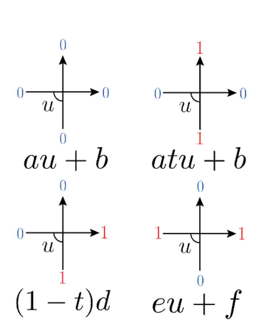
Figure 1: A pictorial description of the $L$-operator (2.20), (2.22). For each configuration, a particular weight is assigned.

3 Wavefunctions and symmetric polynoimals

Here we construct global objects from the local $L$-operators by using the terminology of the quantum inverse scattering method [5, 2, 6]. We first define the monodromy matrix $T_{a}(u)$ from the $L$-operator as

$$T_{a}(u)=L_{aM}(u)\cdots L_{a1}(u) =\begin{pmatrix}A(u)&B(u)\\ C(u)&D(u)\end{pmatrix}_{a}\in\mathrm{End}(W_{a}\otimes V_{1}\otimes\cdots\otimes V_{M}).$$ (3.1)

The matrix elements of the monodromy matrix (see Figure 2 for a pictorial description)

$$A(u)=_{a}\langle 0|T_{a}(u)|0\rangle_{a},$$ (3.2)

$$B(u)=_{a}\langle 0|T_{a}(u)|1\rangle_{a},$$ (3.3)

$$C(u)=_{a}\langle 1|T_{a}(u)|0\rangle_{a},$$ (3.4)

$$D(u)=_{a}\langle 1|T_{a}(u)|1\rangle_{a},$$ (3.5)

are $2^{M}\times 2^{M}$ matrices acting on the tensor product of the quantum spaces $V_{1}\otimes\dots\otimes V_{M}$.

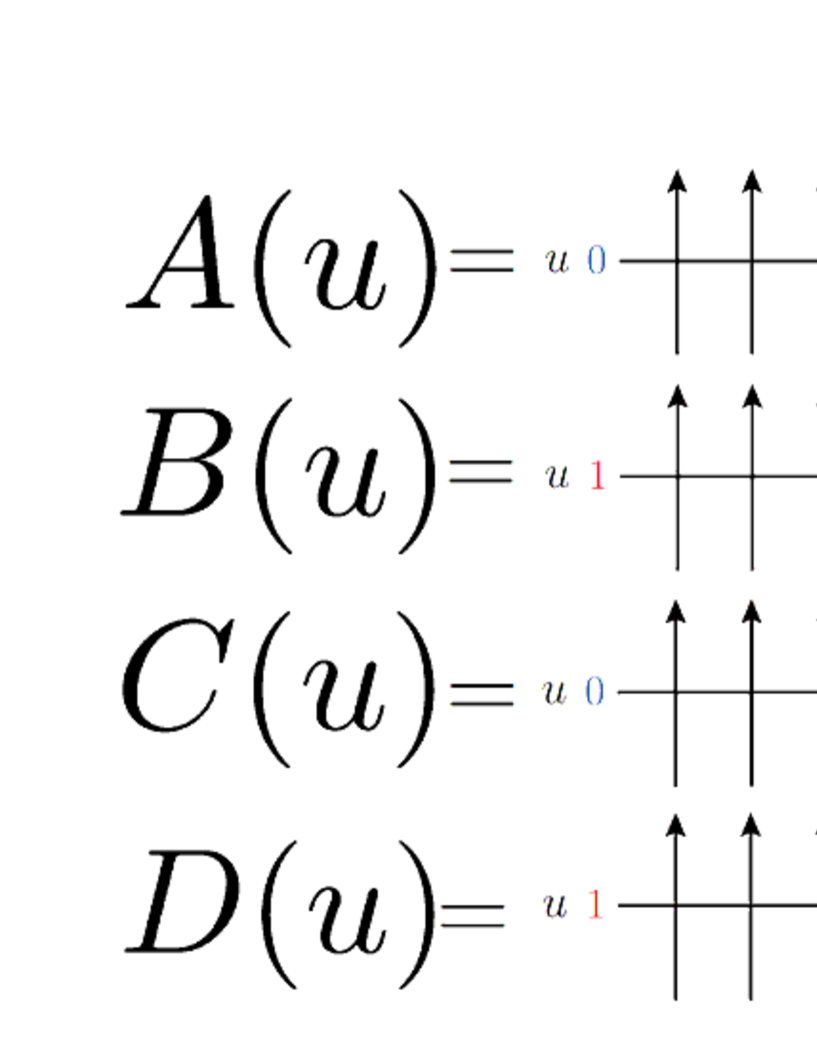
Figure 2: A pictorial description of the $ABCD$-operators which are matrix elements of the monodromy matrix (3.1).

The vector $|0\rangle$, which forms one of the orthonormal basis of $V$, can be interpreted as a state with no particle (hole state). The other vector $|1\rangle$ is interpreted as a particle-occupied state. From the ice rule of the $L$-operator, one easily finds that a single $B$-operator plays the role of creating a particle in the quantum space. Likewise, a single $C$-operator annihilates a particle in the quantum space. To create $N$-particle, $N$-hole states and their duals, we introduce the following vacuum and particle-occupied states

$$|\Omega\rangle :=|0^{M}\rangle:=|0\rangle_{1}\ \otimes\dots\otimes|0\rangle_{M},$$ (3.6)

$$\langle\Omega| :=\langle 0^{M}|:={}_{1}\langle 0|\otimes\dots\otimes{}_{M}\langle 0|,$$ (3.7)

$$\langle 1\cdots M| :=\langle 1^{M}|:={}_{1}\langle 1|\otimes\dots\otimes{}_{M}\langle 1|,$$ (3.8)

$$|1\cdots M\rangle :=|1^{M}\rangle:=|1\rangle_{1}\ \otimes\dots\otimes|1\rangle_{M}.$$ (3.9)

We call $|\Omega\rangle$ ($\langle\Omega|$) as the (dual) vacuum state since there are no particles, and $|1\cdots M\rangle$ ($\langle 1\cdots M|$) as the (dual) particle-occupied state since all the sites are filled with particles.

One can define an $N$-particle state, a dual $N$-particle state, an $N$-hole state and a dual $N$-hole state by acting $N$ $B$- and $C$-operators on the vacuum state, particle-occupied state and their duals

$$|\psi(\{u\}_{N})\rangle =B(u_{N})\cdots B(u_{1})|\Omega\rangle,$$ (3.10)

$$\langle\psi(\{u\}_{N})| =\langle\Omega|C(u_{1})\cdots C(u_{N}),$$ (3.11)

$$\langle\phi(\{u\}_{N})| =\langle 1\cdots M|B(u_{1})\cdots B(u_{N}),$$ (3.12)

$$|\phi(\{u\}_{N})\rangle =C(u_{N})\cdots C(u_{1})|1\cdots M\rangle.$$ (3.13)

For example, $|\psi(\{u\}_{N})\rangle$ (3.10) is an $N$-particle state since $N$ $B$-operators are acting on the vacuum state with no particles. The states (3.10), (3.11), (3.12) and (3.13) are sometimes called as off-shell Bethe vectors. This is because if one imposes a set of constraints (Bethe ansatz equation) on the spectral parameters $u_{j}$ $(j=1,\dots,N)$, the states (3.10), (3.11), (3.12) and (3.13) become eigenvectors of the transfer matrix $t(u):=\mathrm{Tr}_{a}T_{a}(u)=A(u)+D(u)$ which is a generating function of conserved quantities such as the Hamiltonian.

To define wavefunctions, one also needs to introduce vectors which label the configuration of particles. Namely, we define the following particle state and its dual

$$|x_{1}\cdots x_{N}\rangle =\prod_{j=1}^{N}\sigma^{-}_{x_{j}}(|0\rangle_{1}\otimes\cdots\otimes|0\rangle_{M}),$$ (3.14)

$$\langle x_{1}\cdots x_{N}| =(_{1}\langle 0|\otimes\cdots\otimes{}_{M}\langle 0|)\prod_{j=1}^{N}\sigma^{+}_{x_{j}},$$ (3.15)

which are states labelling the configurations of particles $1\leq x_{1}<x_{2}<\cdots<x_{N}\leq M$. Likewise, we introduce vectors describing hole configurations $1\leq\overline{x_{1}}<\overline{x_{2}}<\cdots<\overline{x_{N}}\leq M$

$$|\overline{x_{1}}\cdots\overline{x_{N}}\rangle =\prod_{j=1}^{N}\sigma^{+}_{x_{j}}(|1\rangle_{1}\otimes\cdots\otimes|1\rangle_{M}),$$ (3.16)

$$\langle\overline{x_{1}}\cdots\overline{x_{N}}| =(_{1}\langle 1|\otimes\cdots\otimes{}_{M}\langle 1|)\prod_{j=1}^{N}\sigma^{-}_{x_{j}}.$$ (3.17)

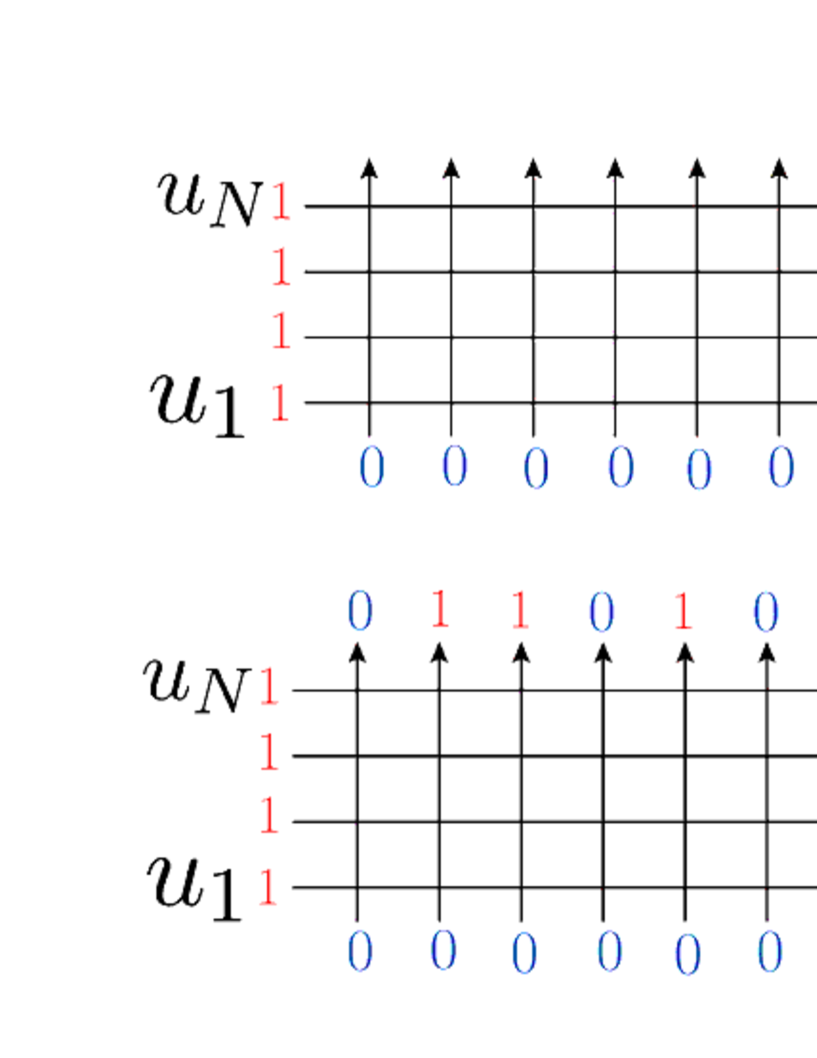
Figure 3: Pictorial descriptions of an $N$-particle state $B(u_{4})B(u_{3})B(u_{2})B(u_{1})|\Omega\rangle$ (top) and a wavefunction $\langle 2,3,5,8|B(u_{4})B(u_{3})B(u_{2})B(u_{1})|\Omega\rangle$ (bottom).

Now we are in a position to define the wavefunctions. The wavefunctions are defined as the overlap between the (dual) $N$-particle ($N$-hole) states (3.10), (3.11), (3.12), (3.13) and the (dual) particle (hole) states (3.14), (3.15), (3.16), (3.17) (see Figure 3 for graphical descriptions of the $N$-particle states and the wavefunctions)

$$\langle x_{1}\cdots x_{N}|\psi(\{u\}_{N})\rangle =\langle x_{1}\cdots x_{N}|B(u_{N})\cdots B(u_{1})|\Omega\rangle,$$ (3.18)

$$\langle\psi(\{u\}_{N})|x_{1}\cdots x_{N}\rangle =\langle\Omega|C(u_{1})\cdots C(u_{N})|x_{1}\cdots x_{N}\rangle,$$ (3.19)

$$\langle\phi(\{u\}_{N})|\overline{x_{1}}\cdots\overline{x_{N}}\rangle =\langle 1\cdots M|B(u_{1})\cdots B(u_{N})|\overline{x_{1}}\cdots\overline{x_{N}}\rangle,$$ (3.20)

$$\langle\overline{x_{1}}\cdots\overline{x_{N}}|\phi(\{u\}_{N})\rangle =\langle\overline{x_{1}}\cdots\overline{x_{N}}|C(u_{N})\cdots C(u_{1})|1\cdots M\rangle.$$ (3.21)

Note that if one fixes a particular $L$-operator, the corresponding wavefunctions are fixed. Before stating the theorem on the exact expressions of the wavefunctions, we first introduce four types of symmetric polynomials.

Definition 3.1.

For a particle configuration $x=(x_{1},x_{2},\dots,x_{N})\ (1\leq x_{1}<x_{2}<\cdots<x_{N}\leq M)$, we define symmetric polynomials $G_{x}(u_{1},\dots,u_{N})$ and $\overline{G}_{x}(u_{1},\dots,u_{N})$ of $u_{1},\dots,u_{N}$ as

$$G_{x}(u_{1},\dots,u_{N})= \prod_{j=1}^{N}\frac{(1-t)cu_{j}(au_{j}+b)^{M}}{eu_{j}+f}\prod_{1\leq j<k\leq N}\frac{tu_{j}-u_{k}}{u_{j}-u_{k}}$$

$$\times\sum_{\sigma\in S_{N}}\prod_{\begin{subarray}{c}1\leq j<k\leq N\\ \sigma(j)>\sigma(k)\end{subarray}}\frac{u_{\sigma(k)}-tu_{\sigma(j)}}{tu_{\sigma(k)}-u_{\sigma(j)}}\prod_{j=1}^{N}\Bigg{(}\frac{eu_{\sigma(j)}+f}{au_{\sigma(j)}+b}\Bigg{)}^{x_{j}},$$ (3.22)

$$\overline{G}_{x}(u_{1},\dots,u_{N})= \prod_{j=1}^{N}\frac{(1-t)d(eu_{j}+f)^{M}}{au_{j}+b}\prod_{1\leq j<k\leq N}\frac{u_{j}-tu_{k}}{u_{j}-u_{k}}$$

$$\times\sum_{\sigma\in S_{N}}\prod_{\begin{subarray}{c}1\leq j<k\leq N\\ \sigma(j)>\sigma(k)\end{subarray}}\frac{tu_{\sigma(k)}-u_{\sigma(j)}}{u_{\sigma(k)}-tu_{\sigma(j)}}\prod_{j=1}^{N}\Bigg{(}\frac{au_{\sigma(j)}+b}{eu_{\sigma(j)}+f}\Bigg{)}^{x_{j}}.$$ (3.23)

For a hole configuration $\overline{x}=(\overline{x_{1}},\overline{x_{2}},\dots,\overline{x_{N}})\ (1\leq\overline{x_{1}}<\overline{x_{2}}<\cdots<\overline{x_{N}}\leq M)$, we define symmetric polynomials $H_{\overline{x}}(u_{1},\dots,u_{N})$ and $\overline{H}_{\overline{x}}(u_{1},\dots,u_{N})$ of $u_{1},\dots,u_{N}$ as

$$H_{\overline{x}}(u_{1},\dots,u_{N})= \prod_{j=1}^{N}\frac{(1-t)cu_{j}(atu_{j}+b)^{M}}{eu_{j}+tf}\prod_{1\leq j<k\leq N}\frac{u_{j}-tu_{k}}{t(u_{j}-u_{k})}$$

$$\times\sum_{\sigma\in S_{N}}\prod_{\begin{subarray}{c}1\leq j<k\leq N\\ \sigma(j)>\sigma(k)\end{subarray}}\frac{tu_{\sigma(k)}-u_{\sigma(j)}}{u_{\sigma(k)}-tu_{\sigma(j)}}\prod_{j=1}^{N}\Bigg{(}\frac{eu_{\sigma(j)}+tf}{atu_{\sigma(j)}+b}\Bigg{)}^{\overline{x_{j}}},$$ (3.24)

$$\overline{H}_{\overline{x}}(u_{1},\dots,u_{N})= \prod_{j=1}^{N}\frac{(1-t)d(eu_{j}+tf)^{M}}{atu_{j}+b}\prod_{1\leq j<k\leq N}\frac{tu_{j}-u_{k}}{t(u_{j}-u_{k})}$$

$$\times\sum_{\sigma\in S_{N}}\prod_{\begin{subarray}{c}1\leq j<k\leq N\\ \sigma(j)>\sigma(k)\end{subarray}}\frac{u_{\sigma(k)}-tu_{\sigma(j)}}{tu_{\sigma(k)}-u_{\sigma(j)}}\prod_{j=1}^{N}\Bigg{(}\frac{atu_{\sigma(j)}+b}{eu_{\sigma(j)}+tf}\Bigg{)}^{\overline{x_{j}}}.$$ (3.25)

We prove the correspondences between the wavefunctions (3.18), (3.19), (3.20), (3.21) constructed from the $L$-operator (2.20), (2.22) and the symmetric polynomials (3.22), (3.23), (3.24), (3.25).

Theorem 3.2.

The wavefunctions (3.18), (3.19), (3.20), (3.21) constructed from the $L$-operator (2.20), (2.22) are expressed by the symmetric polynomials (3.22), (3.23), (3.24), (3.25) as follows:

$$\langle x_{1}\cdots x_{N}|\psi(\{u\}_{N})\rangle =G_{x}(u_{1},\dots,u_{N}),$$ (3.26)

$$\langle\psi(\{u\}_{N})|x_{1}\cdots x_{N}\rangle =\overline{G}_{x}(u_{1},\dots,u_{N}),$$ (3.27)

$$\langle\phi(\{u\}_{N})|\overline{x_{1}}\cdots\overline{x_{N}}\rangle =H_{\overline{x}}(u_{1},\dots,u_{N}),$$ (3.28)

$$\langle\overline{x_{1}}\cdots\overline{x_{N}}|\phi(\{u\}_{N})\rangle =\overline{H}_{\overline{x}}(u_{1},\dots,u_{N}).$$ (3.29)

Let us give here some comments. From the right hand side of the expression (3.26), it is hard to see that it is a symmetric polynomial in $u_{j}$. However, once the correspondence is proven, the symmetry can be shown from the fact that the left hand side $\langle x_{1}\cdots x_{N}|\psi(\{u\}_{N})\rangle=\langle x_{1}\cdots x_{N}|B(u_{N})\cdots B(u_{1})|\Omega\rangle$ is symmetric in $u_{j}$ since the $B$-operators form a commutative family ${[}B(u_{j}),B(u_{k}){]}=0$. The commutativity of the $B$-operators is an immediate consequence of the $RLL$ relation (2.15).

We remark that similar results for (3.26) in Theorem 3.2 have been obtained for the case of $q$-boson models [8, 20, 22, 24, 25, 26, 31] by different methods in this paper. We give a proof of Theorem 3.2 by using the matrix product method and the domain wall boundary partition function in the next two sections. We also mention that the $q$-boson models treated in those papers have fewer free parameters (special cases of the parameters $t,a,b,c,d,e,f$ under the constraints (2.22)) than the vertex model treated in this paper. It is interesting to find the corresponding $q$-boson model which is the counterpart of the spin-1/2 vertex model in this paper. A special case of the correspondence between the wavefunctions of the boson model and the spin-1/2 vertex model is given in [8].

The parameters $a$, $b$, $c$, $d$, $e$ and $f$ of the $L$-operator (2.20) satisfy the constraints (2.22). In particular, it seems that the following specialization $a=1$, $b=t\beta$, $c=1$, $d=1$, $e=-\beta^{-1}$, $f=-1$ is important. Under this specialization, the $L$-operator is written as

$$L_{aj}(u)=\left(\begin{array}[]{cccc}u+t\beta&0&0&0\\ 0&t(u+\beta)&(1-t)u&0\\ 0&1-t&\beta^{-1}u-1&0\\ 0&0&0&-\beta^{-1}u-t\end{array}\right).$$ (3.34)

The wavefunction (3.26) is now given by the symmetric polynomials as

$$\langle x_{1}\cdots x_{N}|\psi(\{u\}_{N})\rangle= \prod_{j=1}^{N}\frac{(1-t)u_{j}(u_{j}+t\beta)^{M}}{-\beta^{-1}u_{j}-1}\prod_{1\leq j<k\leq N}\frac{tu_{j}-u_{k}}{u_{j}-u_{k}}$$

$$\times\sum_{\sigma\in S_{N}}\prod_{\begin{subarray}{c}1\leq j<k\leq N\\ \sigma(j)>\sigma(k)\end{subarray}}\frac{u_{\sigma(k)}-tu_{\sigma(j)}}{tu_{\sigma(k)}-u_{\sigma(j)}}\prod_{j=1}^{N}\Bigg{(}\frac{-\beta^{-1}u_{\sigma(j)}-1}{u_{\sigma(j)}+t\beta}\Bigg{)}^{x_{j}}.$$ (3.35)

If one furthermore set the parameter of the quantum group $t$ to $t=0$, the six-vertex model reduces to the five-vertex model investigated in [7] (up to gauge transformation, see also [28] for a model with inhomogeneties), whose wavefunction becomes the Grothendieck polynomials

$$\langle x_{1}\cdots x_{N}|\psi(\{u\}_{N})\rangle= \prod_{j=1}^{N}\frac{u_{j}^{M+1}}{-\beta^{-1}u_{j}-1}\prod_{1\leq j<k\leq N}\frac{-u_{k}}{u_{j}-u_{k}}$$

$$\times\sum_{\sigma\in S_{N}}\prod_{\begin{subarray}{c}1\leq j<k\leq N\\ \sigma(j)>\sigma(k)\end{subarray}}\frac{-u_{\sigma(k)}}{u_{\sigma(j)}}\prod_{j=1}^{N}(-\beta^{-1}-u_{\sigma(j)}^{-1})^{x_{j}}$$

$$= \prod_{j=1}^{N}\frac{u_{j}^{M}}{-\beta^{-1}u_{j}-1}\prod_{1\leq j<k\leq N}\frac{1}{u_{k}-u_{j}}$$

$$\times\sum_{\sigma\in S_{N}}\mathrm{sgn}(\sigma)\prod_{j=1}^{N}u_{j}^{j}\prod_{\begin{subarray}{c}1\leq j<k\leq N\\ \sigma(j)>\sigma(k)\end{subarray}}\frac{u_{\sigma(k)}}{u_{\sigma}(j)}\prod_{j=1}^{N}(-\beta^{-1}-u_{\sigma(j)}^{-1})^{x_{j}}$$

$$= \frac{\prod_{j=1}^{N}u_{j}^{M}(-\beta^{-1}u_{j}-1)^{-1}}{\prod_{1\leq j<k\leq N}(u_{k}-u_{j})}\mathrm{det}_{N}(u_{j}^{k}(-\beta^{-1}-u_{j}^{-1})^{x_{k}})$$

$$= (-\beta)^{-N(N-1)/2}\prod_{j=1}^{N}u_{j}^{M}G_{\lambda}(\boldsymbol{z};\beta).$$ (3.36)

Here, $G_{\lambda}(\boldsymbol{z};\beta)$ is the $\beta$-Grothendieck polynomials of the Grassmannian vraiety $\mathrm{Gr}(M,N)$ [9, 10, 11, 12, 13, 14], which is known to have the following determinant form

$$G_{\lambda}(\boldsymbol{z};\beta)=\frac{\mathrm{det}_{N}(z_{j}^{\lambda_{k}+N-k}(1+\beta z_{j})^{k-1})}{\prod_{1\leq j<k\leq N}(z_{j}-z_{k})}.$$ (3.37)

In this correspondence between the wavefunctions and the Grothendieck polynomials (3.36), the symmetric variables $\boldsymbol{z}=\{z_{1},\dots,z_{N}\}$ for the Grothendieck polynomials and the spectral parameters $u_{1},\dots,u_{N}$ of the wavefunction are related by the correspondence $z_{j}=-\beta^{-1}-u_{j}^{-1}$, $j=1,\dots,N$. For each Young diagram $\lambda=(\lambda_{1},\lambda_{2},\dots,\lambda_{N})\in\mathbb{Z}^{N}$ ($M-N\geq\lambda_{1}\geq\lambda_{2}\geq\dots\geq\lambda_{N}\geq 0$) there is a corresponding configuration of particles $|x_{1}\cdots x_{N}\rangle$ ($1\leq x_{1}<x_{2}<\cdots<x_{N}\leq M$) by the translation rule $\lambda_{j}=x_{N-j+1}-N+j-1$, $j=1,\dots,N$.

From this observation, one can see that the symmetric polynomials (3.22) giving the correspondence (3.26) can be regarded as a quantum group deformation of the Grothendieck polynomials.

We prove (3.26) in the next two sections. Before ending this section, we check (3.26) by an example.

Example Let us check (3.26) for the case $M=4$, $N=2$, $x_{1}=2$, $x_{2}=4$. One finds from the graphical description of the $L$-operator (see Figures 4, 5 and 6 for the graphical description needed to calculate the left hand side) that the left hand side of (3.26) is given by

$$(L.H.S) =(eu_{1}+f)(eu_{2}+f)(1-t)^{2}c^{2}u_{1}u_{2}X,$$

$$X =(eu_{1}+f)^{2}(au_{2}+b)(atu_{2}+b)+(1-t)^{2}cdu_{2}(au_{1}+b)(eu_{1}+f)$$

$$+(au_{1}+b)^{2}(eu_{2}+f)(eu_{2}+tf).$$ (3.38)

On the other hand, the right hand side is given by

$$(R.H.S) =(eu_{1}+f)(eu_{2}+f)(1-t)^{2}c^{2}u_{1}u_{2}Y,$$

$$Y =\frac{1}{u_{1}-u_{2}}\{(au_{1}+b)^{2}(eu_{2}+f)^{2}(tu_{1}-u_{2})+(eu_{1}+f)^{2}(au_{2}+b)^{2}(u_{1}-tu_{2})\}.$$ (3.39)

Calculating the difference of both hand sides, one gets

$$(L.H.S)-(R.H.S) =(eu_{1}+f)(eu_{2}+f)(1-t)^{2}c^{2}u_{1}u_{2}(X-Y),$$ (3.40)

$$X-Y =bf(t-1)(be-af+(t-1)cd)u_{2}$$

$$+(be+af)(t-1)(be-af+(t-1)cd)u_{1}u_{2}$$

$$+ae(t-1)(be-af+(t-1)cd)u_{1}^{2}u_{2}.$$ (3.41)

Using the relations $cd+af=0$ and $tcd+be=0$, one finds $X-Y=0$, and thus both hand sides of (3.26) are checked to be equal.

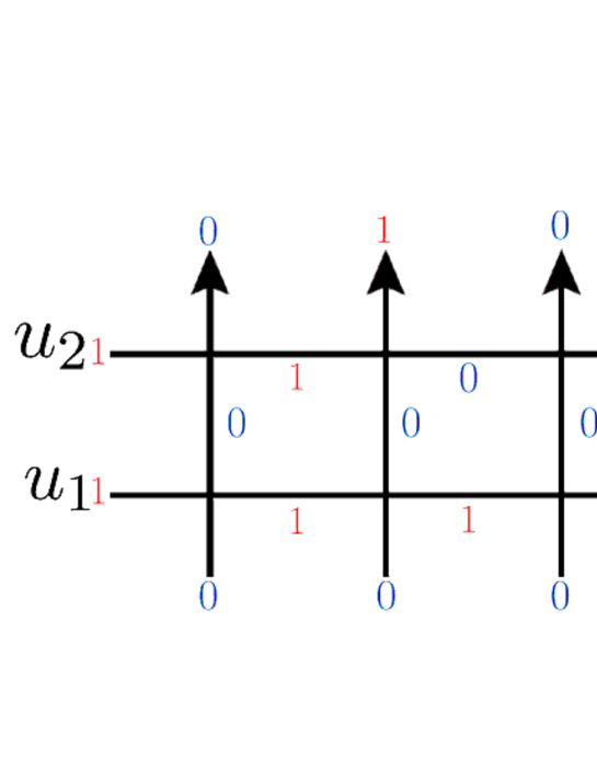
Figure 4: One of the states making a contribution of a factor $(eu_{1}+f)(eu_{2}+f)(1-t)cu_{2}(au_{2}+b)(atu_{2}+b)(eu_{1}+f)(eu_{1}+f)(1-t)cu_{1}$ to the wavefunction $\langle 2,4|B(u_{2})B(u_{1})|\Omega\rangle$.

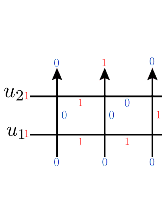
Figure 5: One of the states making a contribution of a factor $(eu_{1}+f)(eu_{2}+f)(1-t)cu_{2}(1-t)d(1-t)cu_{2}(eu_{1}+f)(1-t)cu_{1}(au_{1}+b)$ to the wavefunction $\langle 2,4|B(u_{2})B(u_{1})|\Omega\rangle$.

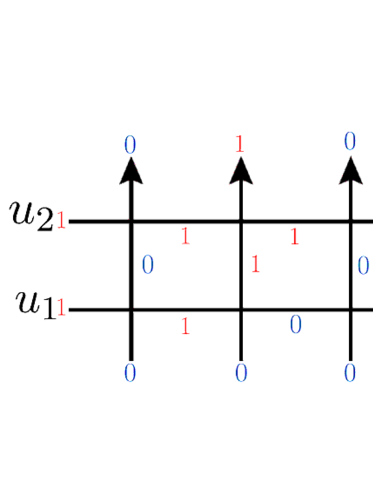
Figure 6: One of the states making a contribution of a factor $(eu_{1}+f)(eu_{2}+f)(eu_{2}+tf)(eu_{2}+f)(1-t)cu_{2}(1-t)cu_{1}(au_{1}+b)(au_{1}+b)$ to the wavefunction $\langle 2,4|B(u_{2})B(u_{1})|\Omega\rangle$.

4 Matrix product representation

In this section, we prove (3.26) in Theorem 3.2 by using the matrix product method and the domain wall boundary partition function. The same strategy was used in [7] to investigate the relation between the wavefunction of an integrable five-vertex model and the Grothendieck polynomials, and in [33, 19] to analyze the relation between the wavefunctions of the Felderhof model and the Schur polynomials. The results for the domain wall boundary partition function used in this section is proved in the next section. The other corresopndences (3.27), (3.28) and (3.29) in Theorem 3.2 can be proved in the same way. We assume the parameters in the $L$-operator $a,b,c,d,e,f$ to be nonzero and $t\neq 1$ since one sometimes needs this assumption in the proof.

The strategy of the proof is as follows. We first rewrite the wavefunction
$\langle x_{1}\cdots x_{N}|\psi(\{u\}_{N})\rangle$ into a matrix product form, following [41, 42], and show that the wavefunction can be expressed as

$$\langle x_{1}\cdots x_{N}|\psi(\{u\}_{N})\rangle= K\sum_{\sigma\in S_{N}}\prod_{\begin{subarray}{c}1\leq j<k\leq N\\ \sigma(j)>\sigma(k)\end{subarray}}\frac{u_{\sigma(k)}-tu_{\sigma(j)}}{tu_{\sigma(k)}-u_{\sigma(j)}}\prod_{j=1}^{N}\Bigg{(}\frac{eu_{\sigma(j)}+f}{au_{\sigma(j)}+b}\Bigg{)}^{x_{j}},$$ (4.1)

where $K$ is a prefactor which does not depend on the particle configurations $x=(x_{1},\dots,x_{N})$ of the wavefunction. Next, by evaluating the exact form of a particular wavefunction
$\langle 1\cdots N|\psi(\{u\}_{N})\rangle$ with the help of the analysis on the domain wall boundary partition function, we show that the prefactor $K$ in (4.1) is given by the following form

$$K=\prod_{j=1}^{N}\frac{(1-t)cu_{j}(au_{j}+b)^{M}}{eu_{j}+f}\prod_{1\leq j<k\leq N}\frac{tu_{j}-u_{k}}{u_{j}-u_{k}},$$ (4.2)

which concludes the proof of (3.26).

Proof.

Let us begin to compute the wavefunction
$\langle x_{1}\cdots x_{N}|\psi(\{u\}_{N})\rangle=\langle x_{1}\cdots x_{N}|\prod_{j=1}^{N}B(u_{j})|\Omega\rangle$. We first rewrite it into the matrix product representation. With the help of its graphical description, one finds that the wavefunction can be written as

$$\langle x_{1}\cdots x_{N}|\prod_{j=1}^{N}B(u_{j})|\Omega\rangle=\operatorname{Tr}_{W^{\otimes N}}\left[Q\langle x_{1}\cdots x_{N}|\prod_{a=1}^{N}T_{a}(u_{a})|\Omega\rangle\right],$$ (4.3)

where $Q=|1^{N}\rangle\langle 0^{N}|$ is an operator acting on the tensor product of auxiliary spaces $W_{1}\otimes\dots\otimes W_{N}$. The trace here is also over the auxiliary spaces.

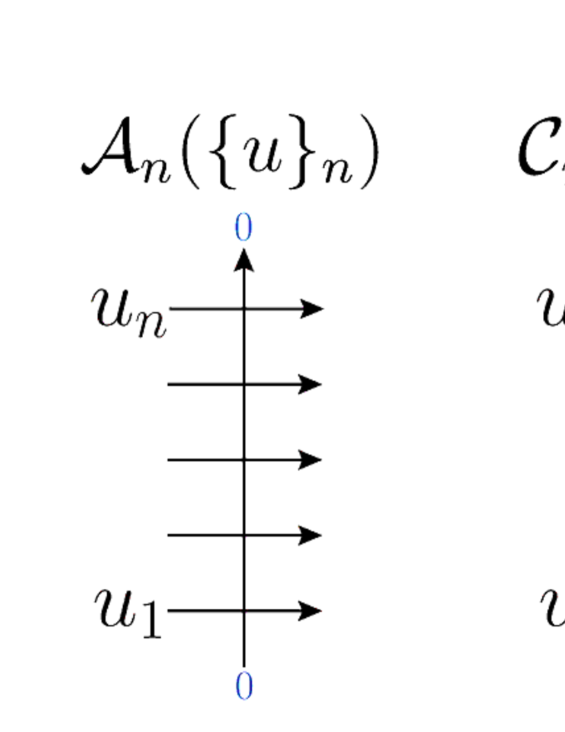
Figure 7: A graphical representation of the matrix elements $\mathcal{A}_{n}(\{u\}_{n})$ and $\mathcal{C}_{n}(\{u\}_{n})$ of the monodromy matrix $\mathcal{T}_{j}(\{u\}_{n})$.

Next we change the viewpoint of the monodromy matrices from the original one $T_{a}(u_{a})\in\mathrm{End}(W_{a}\otimes V_{1}\otimes\cdots\otimes V_{M})$ to the following one

$$\mathcal{T}_{j}(\{u\}_{N}):=\prod_{a=1}^{N}L_{aj}(u_{a})\in\operatorname{End}(W^{\otimes N}\otimes V_{j}),$$ (4.4)

which can be regarded as a monodromy matrix consisting of $L$-operators acting on the same quantum space $V_{j}$ (but acting on different auxiliary spaces). The monodromy matrix $\mathcal{T}_{j}(\{u\}_{N})$ is decomposed as

$$\mathcal{T}_{j}(\{u\}_{N}) :=\begin{pmatrix}\mathcal{A}_{N}(\{u\}_{N})&\mathcal{B}_{N}(\{u\}_{N})\\ \mathcal{C}_{N}(\{u\}_{N})&\mathcal{D}_{N}(\{u\}_{N})\end{pmatrix}_{j},$$ (4.5)

where the elements ($\mathcal{A}_{N}$, etc.) act on $W_{1}\otimes\dots\otimes W_{N}$ (Figure 7).

Using the matrix elements $\mathcal{A}_{N}(\{u\}_{N})$ and $\mathcal{C}_{N}(\{u\}_{N})$ of the monodromy matrix $\mathcal{T}_{j}(\{u\}_{N})$, one finds the wavefunction (4.3) can be written as

$$\langle x_{1}\cdots x_{N}|\psi(\{u\}_{N})\rangle =\operatorname{Tr}_{W^{\otimes N}}\left[Q\langle x_{1}\cdots x_{N}|\prod_{j=1}^{M}\mathcal{T}_{j}(\{u\}_{N})|\Omega\rangle\right]$$

$$=\operatorname{Tr}_{W^{\otimes N}}\left[Q\mathcal{A}_{N}^{M-x_{N}}\mathcal{C}_{N}\mathcal{A}_{N}^{x_{N}-x_{N-1}-1}\dots\mathcal{C}_{N}\mathcal{A}_{N}^{x_{2}-x_{1}-1}\mathcal{C}_{N}\mathcal{A}_{N}^{x_{1}-1}\right].$$ (4.6)

In order to convert the expression (4.6) to the one (4.1), we derive commutation relations between the operators $\mathcal{A}_{N}$ and $\mathcal{C}_{N}$ (Figure 8).

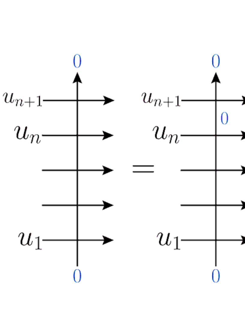
Figure 8: A graphical representation of the recursive relation (4.7) between the monodromy matrices.

First, one finds the following recursive relations for these operators:

$$\mathcal{A}_{n+1}(\{u\}_{n+1})=\begin{pmatrix}au_{n+1}+b&0\\ 0&eu_{n+1}+f\end{pmatrix}\otimes\mathcal{A}_{n}(\{u\}_{n})+\begin{pmatrix}0&0\\ (1-t)d&0\end{pmatrix}\otimes\mathcal{C}_{n}(\{u\}_{n}),$$ (4.7)

$$\mathcal{C}_{n+1}(\{u\}_{n+1})=\begin{pmatrix}0&(1-t)cu_{n+1}\\ 0&0\end{pmatrix}\otimes\mathcal{A}_{n}(\{u\}_{n})+\begin{pmatrix}atu_{n+1}+b&0\\ 0&eu_{n+1}+ft\end{pmatrix}\otimes\mathcal{C}_{n}(\{u\}_{n}),$$ (4.8)

with the initial condition

$$\mathcal{A}_{1}=\begin{pmatrix}au_{1}+b&0\\ 0&eu_{1}+f\end{pmatrix},\quad\mathcal{C}_{1}=\begin{pmatrix}0&(1-t)cu_{1}\\ 0&0\end{pmatrix}.$$ (4.9)

By using the recursive relations (4.7), (4.8) and the initial condition (4.9), one sees that these operators satisfy the following simple algebra.

Lemma 4.1.

There exists a decomposition of $\mathcal{C}_{n}$ : $\mathcal{C}_{n}=\sum_{j=1}^{n}\mathcal{C}_{n}^{(j)}$ such that the following algebraic relations hold for $\mathcal{A}_{n}$ and $\mathcal{C}_{n}^{(j)}$:

$$\mathcal{C}_{n}^{(j)}\mathcal{A}_{n}=\frac{eu_{j}+f}{au_{j}+b}\mathcal{A}_{n}\mathcal{C}_{n}^{(j)},$$ (4.10)

$$(\mathcal{C}_{n}^{(j)})^{2}=0,$$ (4.11)

$$\mathcal{C}_{n}^{(j)}\mathcal{C}_{n}^{(k)}=\frac{(eu_{j}+f)(au_{k}+b)(u_{j}-tu_{k})}{(au_{j}+b)(eu_{k}+f)(tu_{j}-u_{k})}\mathcal{C}_{n}^{(k)}\mathcal{C}_{n}^{(j)},\ \ \ (j\neq k).$$ (4.12)

Proof.

We show by induction on $n$. For $n=1$, from (4.9) $\mathcal{A}_{1}$ is diagonal and one can directly see that the relations are satisfied. For $n$, we assume that $\mathcal{A}_{n}$ is diagonalizable and write the corresponding diagonal matrix as $\mathscr{A}_{n}=G_{n}^{-1}\mathcal{A}_{n}G_{n}$. Also writing $\mathscr{C}_{n}=G_{n}^{-1}\mathcal{C}_{n}G_{n}$ and $\mathscr{C}_{n}=\sum_{j=1}^{n}\mathscr{C}_{n}^{(j)}$, and noting that the algebraic relations above do not depend on the choice of basis, we suppose by the induction hypothesis that the same relations are satisfied by $\mathscr{A}_{n}$ and $\mathscr{C}_{n}^{(j)}$.

We show that the relations hold for $n+1$. To this end, we first construct $G_{n+1}$. Noting from (4.7) that $\mathcal{A}_{n+1}$ is an upper triangular block matrix whose block diagonal elements are written in terms of $\mathcal{A}_{n}$, we assume that $G_{n+1}$ is written as

$$G_{n+1}=\begin{pmatrix}G_{n}&0\\ G_{n}H_{n}&G_{n}\end{pmatrix},$$ (4.13)

where $2n\times 2n$ matrix $H_{n}$ remains to be determined. Using the induction hypothesis for $n$, one obtains

$$G_{n+1}^{-1}\mathcal{A}_{n+1}G_{n+1}$$

$$= \begin{pmatrix}(au_{n+1}+b)\mathscr{A}_{n}&0\\ (eu_{n+1}+f)\mathscr{A}_{n}H_{n}+(1-t)d\mathscr{C}_{n}-(au_{n+1}+b)H_{n}\mathscr{A}_{n}&(eu_{n+1}+f)\mathscr{A}_{n}\end{pmatrix}.$$ (4.14)

The above matrix is guaranteed to be diagonal when

$$(eu_{n+1}+f)\mathscr{A}_{n}H_{n}+(1-t)d\mathscr{C}_{n}-(au_{n+1}+b)H_{n}\mathscr{A}_{n}=0.$$ (4.15)

Utilizing the above relation and recalling $\mathscr{A}_{n}$ and $\mathscr{C}^{(j)}_{n}$ satisfy the relation same as that in (4.10), one finds $H_{n}$ is expressed as

$$H_{n}=\mathscr{A}^{-1}_{n}\sum_{j=1}^{n}\frac{au_{j}+b}{c(u_{j}-u_{n+1})}\mathscr{C}_{n}^{(j)}.$$ (4.16)

One thus obtains the diagonal matrix $\mathscr{A}_{n+1}$:

$$\mathscr{A}_{n+1}=\begin{pmatrix}(au_{n+1}+b)\mathscr{A}_{n}&0\\ 0&(eu_{n+1}+f)\mathscr{A}_{n}\end{pmatrix}.$$ (4.17)

The remaining task is to derive $\mathscr{C}_{n+1}^{(j)}$ and to prove the relations (4.10)–(4.12) hold for $n+1$. Combining (4.8), (4.13) and (4.16), and also inserting the relations (4.11) and (4.12), one arrives at $\mathscr{C}_{n+1}=\sum_{j=1}^{n+1}\mathscr{C}_{n+1}^{(j)}$ where

$$\mathscr{C}_{n+1}^{(j)}=\begin{cases}\displaystyle\frac{1}{u_{j}-u_{n+1}}\begin{pmatrix}(u_{j}-tu_{n+1})(au_{n+1}+b)\mathscr{C}_{n}^{(j)}&0\\ 0&(tu_{j}-u_{n+1})(eu_{n+1}+f)\mathscr{C}_{n}^{(j)}\end{pmatrix}\\[17.07164pt] \text{ for $1\leq j\leq n$}\\[17.07164pt] \begin{pmatrix}0&(1-t)cu_{n+1}\mathscr{A}_{n}\\ 0&0\end{pmatrix}\text{ for $j=n+1$}\end{cases}.$$ (4.18)

Finally recalling that $\mathscr{A}_{n}$ and $\mathscr{C}_{n}^{(j)}$ are supposed to satisfy the relations (4.10)–(4.12) and using the explicit form of $\mathscr{A}_{n+1}$ (4.17) and $\mathscr{C}_{n+1}^{(j)}$ (4.18), one sees they satisfy the same algebraic relations as those in (4.10)–(4.12) for $n+1$. ∎

Due to the algebraic relations (4.10), (4.11) and (4.12) in Lemma 4.1, the matrix product form for the wavefunction (4.6) can be rewritten into the following form.

Proposition 4.2.

The wavefunction $\langle x_{1}\cdots x_{N}|\psi(\{u\}_{N})\rangle$ is expressed in the following form

$$\langle x_{1}\cdots x_{N}|\psi(\{u\}_{N})\rangle= K\sum_{\sigma\in S_{N}}\prod_{\begin{subarray}{c}1\leq j<k\leq N\\ \sigma(j)>\sigma(k)\end{subarray}}\frac{u_{\sigma(k)}-tu_{\sigma(j)}}{tu_{\sigma(k)}-u_{\sigma(j)}}\prod_{j=1}^{N}\Bigg{(}\frac{eu_{\sigma(j)}+f}{au_{\sigma(j)}+b}\Bigg{)}^{x_{j}}.$$ (4.19)

Here, $S_{N}$ denotes the symmetric group of order $N$, and the prefactor $K$ is given by

$$K=\prod_{j=1}^{N}\Bigg{(}\frac{au_{j}+b}{eu_{j}+f}\Bigg{)}^{j}\operatorname{Tr}_{W^{\otimes N}}\left[Q\mathcal{A}_{N}^{M-N}\mathcal{C}_{N}^{(N)}\dots\mathcal{C}_{N}^{(1)}\right].$$ (4.20)

What remains to be done to show (3.26) is to determine the explicit form of the prefactor $K$ in (4.19). From the expressions (4.19) and (4.20), one sees that the information of the particle configuration $x=(x_{1},x_{2},\dots,x_{N})$ is encoded in the determinant, while the overall factor $K$ is independent of the configuration. This fact means that one can determine the factor $K$ by evaluating the overlap for a particular particle configuration. In fact, we find the following explicit form of the prefactor $K$ by finding an explicit expression of the wavefunction $\langle x_{1}\cdots x_{N}|\psi(\{u\}_{N})\rangle$ for the case $x_{j}=j$ ($1\leq j\leq N$):

Proposition 4.3.

The prefactor $K$ in (4.19) is given by

$$K=\prod_{j=1}^{N}\frac{(1-t)cu_{j}(au_{j}+b)^{M}}{eu_{j}+f}\prod_{1\leq j<k\leq N}\frac{tu_{j}-u_{k}}{u_{j}-u_{k}}.$$ (4.21)

Proof.

We prove Proposition 4.3 by showing

$$\langle 1\cdots N|\psi(\{u\}_{N})\rangle= \prod_{j=1}^{N}\frac{(1-t)cu_{j}(au_{j}+b)^{M}}{eu_{j}+f}\prod_{1\leq j<k\leq N}\frac{tu_{j}-u_{k}}{u_{j}-u_{k}}$$

$$\times\sum_{\sigma\in S_{N}}\prod_{\begin{subarray}{c}1\leq j<k\leq N\\ \sigma(j)>\sigma(k)\end{subarray}}\frac{u_{\sigma(k)}-tu_{\sigma(j)}}{tu_{\sigma(k)}-u_{\sigma(j)}}\prod_{j=1}^{N}\Bigg{(}\frac{eu_{\sigma(j)}+f}{au_{\sigma(j)}+b}\Bigg{)}^{j},$$ (4.22)

since combining (4.22) and Proposition 4.2 for the case $x_{j}=j,\ j=1,\dots,N$ gives (4.21).

We now begin to evaluate a particular wavefunction $\langle 1\cdots N|\psi(\{u\}_{N})\rangle$. From its graphical description, we can easily see that $\langle 1\cdots N|\psi(\{u\}_{N})\rangle$ can be factorized as (see Figure 9)

$$\langle 1\cdots N|\psi(\{u\}_{N})\rangle =Z_{N}(\{u\}_{N})\prod_{j=1}^{N}(au_{j}+b)^{M-N},$$ (4.23)

where $Z_{N}(\{u\}_{N})$ is the domain wall boundary partition function on an $N\times N$ grid

$$Z_{N}(\{u\}_{N}) =\langle 1\cdots N|B_{N}(u_{1})\cdots B_{N}(u_{N})|\Omega\rangle,$$ (4.24)

$$B_{N}(u) ={}_{a}\langle 0|L_{aN}(u)\cdots L_{a1}(u)|1\rangle_{a}.$$ (4.25)

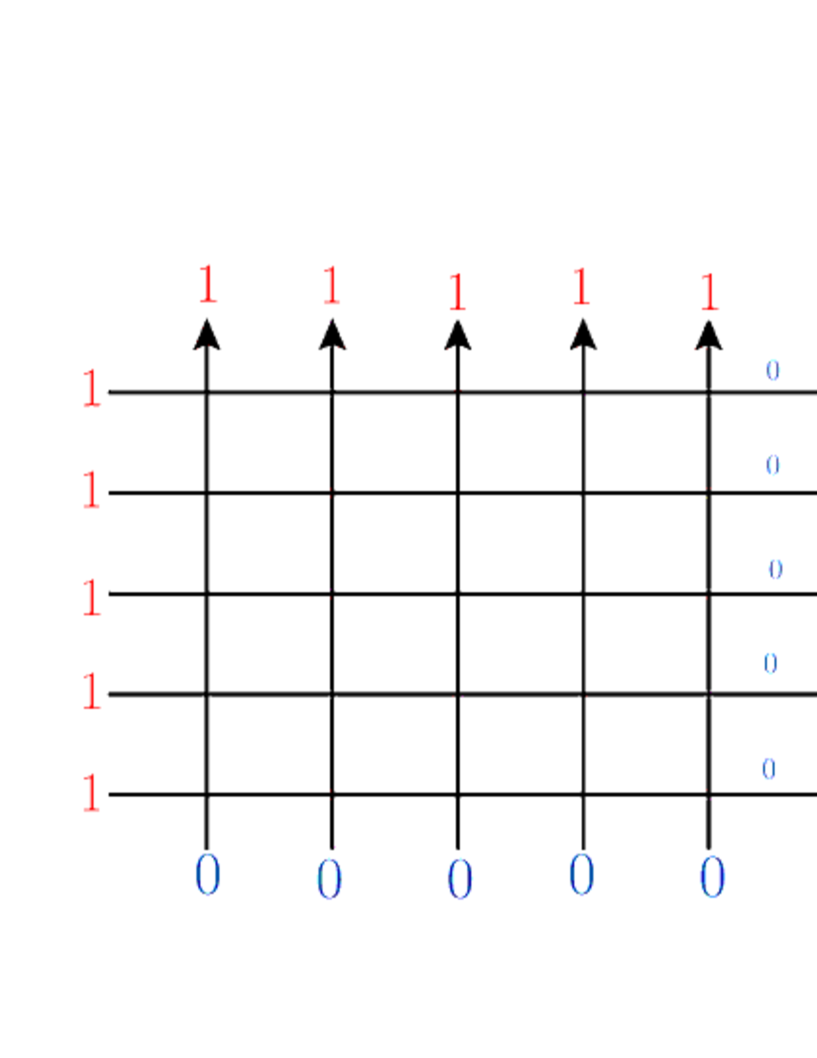
Figure 9: A graphical representation which shows the factorization of the wavefunction $\langle 1\cdots N|\psi(\{u\}_{N})\rangle=Z_{N}(\{u\}_{N})\prod_{j=1}^{N}(au_{j}+b)^{M-N}$ for the case $M=9$, $N=5$. One can easily see from its graphical reprensenation and the ice rule that the inner states of the left part of the wavefunction freeze, and the evaluation of this particular type of wavefunctions reduces to that of the domain wall boundary partition function.

One can show that the domain wall boundary partition function $Z_{N}(\{u\}_{N})$ has an expression given by (5.1), which will be proven in the next section. Inserting (5.1) into (4.23), one gets

$$\langle 1\cdots N|\psi(\{u\}_{N})\rangle= \prod_{j=1}^{N}\frac{(1-t)cu_{j}(au_{j}+b)^{M}}{eu_{j}+f}\prod_{1\leq j<k\leq N}\frac{tu_{j}-u_{k}}{u_{j}-u_{k}}$$

$$\times\sum_{\sigma\in S_{N}}\prod_{\begin{subarray}{c}1\leq j<k\leq N\\ \sigma(j)>\sigma(k)\end{subarray}}\frac{u_{\sigma(k)}-tu_{\sigma(j)}}{tu_{\sigma(k)}-u_{\sigma(j)}}\prod_{j=1}^{N}\Bigg{(}\frac{eu_{\sigma(j)}+f}{au_{\sigma(j)}+b}\Bigg{)}^{j},$$ (4.26)

hence Proposition 4.3 is proved. ∎

Having proved Propostitions 4.2 and 4.3, it immediately follows from the combination of the two propositions that the wavefunction $\langle x_{1}\cdots x_{N}|\psi(\{u\}_{N})\rangle$ is exactly expressed by the symmetric polynomials $G_{x}(u_{1},\dots,u_{N})$, hence (3.26) is proved. ∎

5 Domain wall boundary partition function

In this section, we show the following form for the domain wall boundary partition function $Z_{N}(\{u\}_{N})$ which is used to show (3.26) in the last section.

Theorem 5.1.

The domain wall boundary partition function $Z_{N}(\{u\}_{N})$ has the following form

$$Z_{N}(\{u\}_{N})= \prod_{j=1}^{N}(1-t)cu_{j}\prod_{1\leq j<k\leq N}\frac{tu_{j}-u_{k}}{u_{j}-u_{k}}$$

$$\times\sum_{\sigma\in S_{N}}\prod_{\begin{subarray}{c}1\leq j<k\leq N\\ \sigma(j)>\sigma(k)\end{subarray}}\frac{u_{\sigma(k)}-tu_{\sigma(j)}}{tu_{\sigma(k)}-u_{\sigma(j)}}\prod_{j=1}^{N}(au_{\sigma(j)}+b)^{N-j}\prod_{j=1}^{N}(eu_{\sigma(j)}+f)^{j-1}.$$ (5.1)

We show this expression (5.1) by generalizing the theorem to the case of inhomogeneous domain wall boundary partition function. Namely, we generalize the $L$-opearator by including inhomogeneous parameters $w_{j}$ in the quantum space $V_{j}$, $j=1,\dots,N$

$$L_{aj}(u,w_{j})=\left(\begin{array}[]{cccc}au+bw_{j}&0&0&0\\ 0&atu+bw_{j}&(1-t)cu&0\\ 0&(1-t)dw_{j}&eu+fw_{j}&0\\ 0&0&0&eu+tfw_{j}\end{array}\right),$$ (5.6)

and construct an inhomogeneous generalization of the domain wall boundary partition function $Z_{N}(\{u\}_{N}|\{w\}_{N})$ which is defined as the following:

$$Z_{N}(\{u\}_{N}|\{w\}_{N}) =\langle 1\cdots N|B_{N}(u_{1}|\{w\}_{N})\cdots B_{N}(u_{N}|\{w\}_{N})|\Omega\rangle,$$ (5.7)

$$B_{N}(u|\{w\}_{N}) ={}_{a}\langle 0|L_{aN}(u,w_{N})\cdots L_{a1}(u,w_{1})|1\rangle_{a}.$$ (5.8)

One can show the following expression for the inhomogeneous domain wall boundary partition function.

Theorem 5.2.

The inhomogeneous domain wall boundary partition function $Z_{N}(\{u\}_{N}|\{w\}_{N})$ has the following form:

$$Z_{N}(\{u\}_{N},\{w\}_{N})$$

$$= \prod_{j=1}^{N}(1-t)cu_{j}\prod_{1\leq j<k\leq N}\frac{tu_{j}-u_{k}}{u_{j}-u_{k}}$$

$$\times\sum_{\sigma\in S_{N}}\prod_{\begin{subarray}{c}1\leq j<k\leq N\\ \sigma(j)>\sigma(k)\end{subarray}}\frac{u_{\sigma(k)}-tu_{\sigma(j)}}{tu_{\sigma(k)}-u_{\sigma(j)}}\prod_{1\leq j<k\leq N}(au_{\sigma(j)}+bw_{k})\prod_{1\leq k<j\leq N}(eu_{\sigma(j)}+fw_{k}).$$ (5.9)

Theorem 5.1 follows immediately from Theorem 5.2 by taking the homogeneous limit of the inhomogeneous parameters $w_{j}=1$, $j=1,\dots,N$.

Theorem 5.2 can be proved by using the standard Izergin-Korepin technique [43, 44]. See [45] for the results for the case of the elliptic ABF model. We show the outline of the proof. The Izergin-Korepin technique is to first show properties for the inhomogeneous domain wall boundary partition function $Z_{N}(\{u\}_{N}|\{w\}_{N})=\langle 1\cdots N|B(u_{1}|\{w\}_{N})\cdots B(u_{N}|\{w\}_{N})|\Omega\rangle$ which is given in the proposition below, with the help of its graphical description. Then one next finds the unique desired polynomials satisfying the properties, and conclude that the polynomial is the exact expression for the domain wall boundary partition function.

Proposition 5.3.

The inhomogeneous domain wall boundary partition function $Z_{N}(\{u\}_{N}|\{w\}_{N})$ satisfies the following properties.

(1) $Z_{N}(\{u\}_{N}|\{w\}_{N})$ is a polynomial of degree $N-1$ in $w_{N}$.
(2) $Z_{N}(\{u\}_{N}|\{w\}_{N})$ is symmetric with respect to $u_{j}$, $j=1,\dots,N$.
(3) The case $n=1$ is given by $Z_{1}(u_{1}|w_{1})=(1-t)cu_{1}$. @
(4) The following recursive relations between the domain wall boundary partition functions hold (Figure 10):

$$Z_{N}(\{u\}_{N}|\{w\}_{N})|_{w_{N}=-au_{k}/b}= (1-t)ca^{N-1}u_{k}\prod_{\begin{subarray}{c}j=1\\ j\neq k\end{subarray}}^{N}(tu_{j}-u_{k})\prod_{j=1}^{N-1}(eu_{k}+fw_{j})$$

$$\times Z_{N-1}(\{u_{1},\dots,u_{k-1},u_{k+1},\dots,u_{N}\}|\{w\}_{N-1}).$$ (5.10)

One can show that the following polynomial satisfies the properties (1),(2),(3),(4) of Proposition 5.3

$$F_{N}(\{u\}_{N},\{w\}_{N})$$

$$= \prod_{j=1}^{N}(1-t)cu_{j}\prod_{1\leq j<k\leq N}\frac{tu_{j}-u_{k}}{u_{j}-u_{k}}$$

$$\times\sum_{\sigma\in S_{N}}\prod_{\begin{subarray}{c}1\leq j<k\leq N\\ \sigma(j)>\sigma(k)\end{subarray}}\frac{u_{\sigma(k)}-tu_{\sigma(j)}}{tu_{\sigma(k)}-u_{\sigma(j)}}\prod_{1\leq j<k\leq N}(au_{\sigma(j)}+bw_{k})\prod_{1\leq k<j\leq N}(eu_{\sigma(j)}+fw_{k}).$$ (5.11)

For example, let us consider the property (4). If one sets $w_{N}$ to $w_{N}=-au_{N}/b$, each of the summands labeled by the elements $\sigma\in S_{N}$ not satisfying $\sigma(N)=N$ in the summation of (5.11) always has a zero factor $\prod_{1\leq j<k\leq N}(au_{\sigma(j)}+bw_{k})$=0. Thus, one can restrict the summation to the elements $\sigma$ which satisfy $\sigma(N)=N$. Then it is easy to check that the polynomial $F_{N}(\{u\}_{N},\{w\}_{N})$ satisfies the recursive relation (5.10) for the case $k=N$. Thus we have proved that the inhomogeneous domain wall boundary partition function $Z_{N}(\{u\}_{N}|\{w\}_{N})$ is given by the polynomial $F_{N}(\{u\}_{N},\{w\}_{N})$.

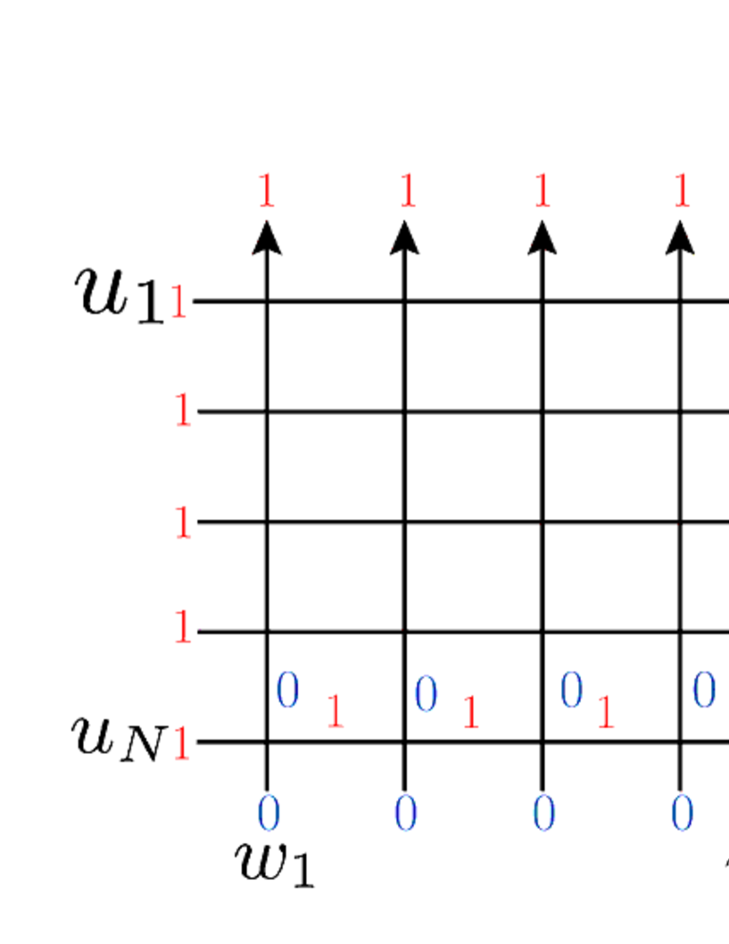
Figure 10: A graphical representation of the recursive relation of the domain wall boundary partition function (5.10) for the case $k=N$.

6 Pairing formulas between the symmetric polynomials

In the following two sections, we make applications of the correspondences between the wavefunctions and the symmetric polynomials. In this section, we prove a pairing formula between the symmetric polynomials $G_{x}(\{u\})$ and $H_{\overline{x}}(\{u\})$. First, we start from the Izergin-Korepin determinant formula [43, 44] of the domain wall boundary partition function $Z_{N}(\{u\}_{N}|\{w\}_{N})$.

Theorem 6.1.

The domain wall boundary partition function $Z_{N}(\{u\}_{N}|\{w\}_{N})$ can be expressed as the following determinant

$$Z_{N}(\{u\}_{N}|\{w\}_{N})= \frac{\prod_{j=1}^{N}(1-t)cu_{j}\prod_{j,k=1}^{N}(au_{j}+bw_{k})(eu_{j}+fw_{k})}{(cd)^{N(N-1)/2}\prod_{1\leq j<k\leq N}(u_{j}-u_{k})(w_{k}-w_{j})}$$

$$\times\mathrm{det}_{N}\Bigg{(}\frac{1}{(au_{j}+bw_{k})(eu_{j}+fw_{k})}\Bigg{)}.$$ (6.1)

This determinant representation (6.1) is more famous than the one (5.9) in the last section. This can also be proven by showing that (6.1) satisfies the Properties (1), (2), (3), (4) of Lemma 5.3.

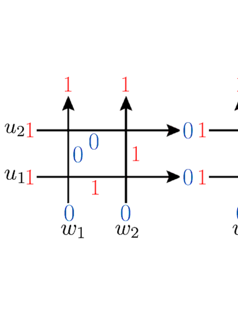
Figure 11: The state on the left and right makes a contribution of a factor $(1-t)cu_{2}(atu_{2}+bw_{2})(eu_{1}+fw_{1})(1-t)cu_{1}$ and $(eu_{2}+tfw_{1})(1-t)cu_{1}(1-t)cu_{2}(au_{1}+bw_{2})$ respectively to the inhomogeneous domain wall boundary partition function $Z_{2}(\{u_{1},u_{2}\}|\{w_{1},w_{2}\})$.

Example By using the definition of the $L$-operator, one can calculate the inhomogeneous domain wall boundary partition function $Z_{2}(\{u_{1},u_{2}\}|\{w_{1},w_{2}\})$ as (see Figure 11) $Z_{2}(\{u_{1},u_{2}\}|\{w_{1},w_{2}\})=(L.H.S)=(1-t)^{2}c^{2}u_{1}u_{2}((atu_{2}+bw_{2})(eu_{1}+fw_{1})+(eu_{2}+tfw_{1})(au_{1}+bw_{2}))$. The right hand side of (6.1) is $(R.H.S)=(1-t)^{2}cd^{-1}u_{1}u_{2}((be+af)(aeu_{1}u_{2}+bfw_{1}w_{2})+abef(u_{1}+u_{2})(w_{1}+w_{2}))$, and one can check the difference becomes

$$(L.H.S)-(R.H.S) =(1-t)^{2}cd^{-1}u_{1}u_{2}((cd+be+af+tcd)(aeu_{1}u_{2}+bfw_{1}w_{2})$$

$$+ af(be+tcd)(u_{1}+u_{2})w_{1}+be(cd+af)(u_{1}+u_{2})w_{2}),$$ (6.2)

which is zero due to the relations $cd+af=0$ and $tcd+be=0$.

By taking the homogeneous limit of the determinant representation (6.1) following Izergin-Coker-Korepin [46], one gets the following determinant form for the partition function without inhomogeneous parameters.

Proposition 6.2.

The homogeneous limit of the determinant representation of the domain wall boundary partition function is expressed as the following determinant

$$Z_{N}(\{u\}_{N})=\frac{\mathrm{det}_{N}((au_{j}+b)^{N}(-f)^{k}(eu_{j}+f)^{N-k}-(eu_{j}+f)^{N}(-b)^{k}(au_{j}+b)^{N-k})}{c^{N(N-1)/2}d^{N(N+1)/2}\prod_{1\leq j<k\leq N}(u_{j}-u_{k})}.$$ (6.3)

Proof.

Let us first examine

$$\frac{1}{\prod_{1\leq j<k\leq N}(w_{k}-w_{j})}\mathrm{det}_{N}\Bigg{(}\frac{1}{(au_{j}+bw_{k})(eu_{j}+fw_{k})}\Bigg{)}.$$ (6.4)

We rewrite the matrix elements $\displaystyle\frac{1}{(au_{j}+bw_{k})(eu_{j}+fw_{k})}$ of the determinant. Assuming $c\neq 0$ and $d\neq 0$ and using $be-af=(1-t)cd$, one finds the following equality

$$\frac{1}{(au_{j}+bw_{k})(eu_{j}+fw_{k})}=\frac{1}{(1-t)cdu_{j}}\frac{b}{au_{j}+bw_{k}}-\frac{1}{(1-t)cdu_{j}}\frac{f}{eu_{j}+fw_{k}},$$ (6.5)

and (6.4) becomes

$$\frac{1}{\prod_{1\leq j<k\leq N}(w_{k}-w_{j})}\mathrm{det}_{N}\Bigg{(}\frac{1}{(au_{j}+bw_{k})(eu_{j}+fw_{k})}\Bigg{)}$$

$$= \frac{1}{((1-t)cd)^{N}\prod_{j=1}^{N}u_{j}\prod_{1\leq j<k\leq N}(w_{k}-w_{j})}\mathrm{det}_{N}\Bigg{(}\frac{b}{bw_{k}+au_{j}}-\frac{f}{fw_{k}+eu_{j}}\Bigg{)}.$$ (6.6)

Taking the limit $w_{1}\to 1$, $w_{2}\to 1,\dots$, $w_{N}\to 1$ successively, one gets the following expression with the help of Taylor expansion

$$\lim_{w_{1},\dots,w_{N}\to 1}\frac{1}{\prod_{1\leq j<k\leq N}(w_{k}-w_{j})}\mathrm{det}_{N}\Bigg{(}\frac{1}{(au_{j}+bw_{k})(eu_{j}+fw_{k})}\Bigg{)}$$

$$= \frac{1}{((1-t)cd)^{N}\prod_{j=1}^{N}u_{j}}\mathrm{det}_{N}\Bigg{(}\frac{f^{k}}{(-f-eu_{j})^{k}}-\frac{b^{k}}{(-b-au_{j})^{k}}\Bigg{)}.$$ (6.7)

Taking the remaining factors into account, one has the homogeneous limit of the partition function

$$Z_{N}(\{u\}_{N})= \frac{\prod_{j=1}^{N}(1-t)cu_{j}(au_{j}+b)^{N}(eu_{j}+f)^{N}}{(cd)^{N(N-1)/2}\prod_{1\leq j<k\leq N}(u_{j}-u_{k})}$$

$$\times\frac{1}{((1-t)cd)^{N}\prod_{j=1}^{N}u_{j}}\mathrm{det}_{N}\Bigg{(}\frac{f^{k}}{(-f-eu_{j})^{k}}-\frac{b^{k}}{(-b-au_{j})^{k}}\Bigg{)}$$

$$= \frac{\mathrm{det}_{N}((au_{j}+b)^{N}(-f)^{k}(eu_{j}+f)^{N-k}-(eu_{j}+f)^{N}(-b)^{k}(au_{j}+b)^{N-k})}{c^{N(N-1)/2}d^{N(N+1)/2}\prod_{1\leq j<k\leq N}(u_{j}-u_{k})}.$$ (6.8)

∎

Example Let us check the case $N=2$. Using the relations $af=-cd$, $be=-tcd$, the right hand side of (6.3) can be rewritten as

$$-(be-af)^{2}(cd^{3})^{-1}u_{1}u_{2}(bf(be+af)+2abef(u_{1}+u_{2})+ae(be+af)u_{1}u_{2})$$

$$= -(t-1)^{2}c^{2}d^{2}(cd^{3})^{-1}u_{1}u_{2}(-(t+1)bfcd+(-cdbe-tcdaf)(u_{1}+u_{2})-(t+1)aecdu_{1}u_{2})$$

$$= (t-1)^{2}c^{2}u_{1}u_{2}((t+1)bf+(be+taf)(u_{1}+u_{2})+(t+1)aeu_{1}u_{2})$$

$$= (1-t)^{2}c^{2}u_{1}u_{2}\{(atu_{2}+b)(eu_{1}+f)+(eu_{2}+tf)(au_{1}+b)\},$$ (6.9)

which finally becomes the expression of $Z_{2}(\{u_{1},u_{2}\})$ calculated from the definition of the $L$-operator.

Now we can prove the following pairing formula for the symmetric polynomials.

Theorem 6.3.

We have the following pairing formula between the symmetric polynomials $G_{x}(u_{M-N+1},\dots,u_{M})$ and $H_{\overline{x}}(u_{1},\dots,u_{M-N})$

$$\sum_{x}H_{\overline{x}}(u_{1},\dots,u_{M-N})G_{x}(u_{M-N+1},\dots,u_{M})$$

$$= \frac{\mathrm{det}_{N}((au_{j}+b)^{N}(-f)^{k}(eu_{j}+f)^{N-k}-(eu_{j}+f)^{N}(-b)^{k}(au_{j}+b)^{N-k})}{c^{N(N-1)/2}d^{N(N+1)/2}\prod_{1\leq j<k\leq N}(u_{j}-u_{k})}.$$ (6.10)

Here, for each term of the product between $G_{x}(u_{M-N+1},\dots,u_{M})$ and $H_{\overline{x}}(u_{1},\dots,u_{M-N})$, the hole configuration $\overline{x}$ of $H_{\overline{x}}(u_{1},\dots,u_{M-N})$ is the complementary part of the particle configuration $x$ of $G_{x}(u_{M-N+1},\dots,u_{M})$. That is, the particle configuration $x=\{x_{1},\dots,x_{N}\}$ and the hole configuration $\overline{x}=\{\overline{x_{1}}\dots\overline{x_{M-N}}\}$ forms a disjoint union of $\{1,2,\dots,N\}$, $x\sqcup\overline{x}=\{1,2\dots,N\}$. The sum in the left hand side of (6.10) is over all particle configurations $x=(1\leq x_{1}<x_{2}<\cdots<x_{N}\leq M)$.

Proof.

The theorem can be shown by combining the two expressions for the domain wall boundary partition function $Z_{N}(\{u\}_{N})$. From Proposition 6.2, one has the direct determinant representation (6.3). Another way of evaluating the domain wall boundary partition function is to insert the completeness relation

$$\sum_{\{x\}}|x_{1}\cdots x_{N}\rangle\langle x_{1}\cdots x_{N}|=\mathrm{Id},$$ (6.11)

between the $B$-operators to get

$$\langle 1\cdots M|B(u_{1})\cdots B(u_{M})|\Omega\rangle$$

$$= \sum_{\{x\}}\langle 1\cdots M|B(u_{1})\cdots B(u_{M-N})|x_{1}\cdots x_{N}\rangle\langle x_{1}\cdots x_{N}|B(u_{M-N+1})\cdots B(u_{M})|\Omega\rangle$$

$$= \sum_{\{x\}}\langle 1\cdots M|B(u_{1})\cdots B(u_{M-N})|\overline{x_{1}}\cdots\overline{x_{M-N}}\rangle\langle x_{1}\cdots x_{N}|B(u_{M-N+1})\cdots B(u_{M})|\Omega\rangle,$$ (6.12)

and use the correspondence between the wavefunctions and the symmetric polynomials (3.26) and (3.28) . Combining the two ways of evaluations, one gets the pairing formula. ∎

One can do the same analysis to give a pairing formula between the symmetric polynomials $\overline{G}_{x}(\{u\})$ and $\overline{H}_{\overline{x}}(\{u\})$ from the dual domain wall boundary partition $\overline{Z_{N}}(\{u\}_{N})$

$$\overline{Z_{N}}(\{u\}_{N}) =\langle\Omega|C_{N}(u_{N})\cdots C_{N}(u_{1})|1\cdots N\rangle,$$ (6.13)

$$C_{N}(u) ={}_{a}\langle 1|L_{aN}(u)\cdots L_{a1}(u)|0\rangle.$$ (6.14)

Again, we start by generalizing to the inhomogeneous version

$$\overline{Z_{N}}(\{u\}_{N}|\{w\}_{N}) =\langle\Omega|C_{N}(u_{N}|\{w\}_{N})\cdots C_{N}(u_{1}|\{w\}_{N})|1\cdots N\rangle,$$ (6.15)

$$C_{N}(u|\{w\}_{N}) ={}_{a}\langle 1|L_{aN}(u,w_{N})\cdots L_{a1}(u,w_{1})|0\rangle.$$ (6.16)

We have the following determinant form.

Theorem 6.4.

The inhomogeneous dual domain wall boundary partition function $\overline{Z_{N}}(\{u\}_{N}|\{w\}_{N})$ can be expressed as the following determinant

$$\overline{Z_{N}}(\{u\}_{N}|\{w\}_{N})= \frac{\prod_{j=1}^{N}(1-t)dw_{j}\prod_{j,k=1}^{N}(atu_{j}+bw_{k})(eu_{j}+tfw_{k})}{(t^{2}cd)^{N(N-1)/2}\prod_{1\leq j<k\leq N}(u_{j}-u_{k})(w_{k}-w_{j})}$$

$$\times\mathrm{det}_{N}\Bigg{(}\frac{1}{(atu_{j}+bw_{k})(eu_{j}+tfw_{k})}\Bigg{)}.$$ (6.17)

By taking the homogeneous limit of the determinant (6.17), one gets the following determinant form for $\overline{Z_{N}}(\{u\}_{N})$.

Proposition 6.5.

The homogeneous limit of the determinant representation of the dual domain wall boundary partition function is expressed as the following determinant

$$\overline{Z_{N}}(\{u\}_{N})=\frac{\mathrm{det}_{N}((eu_{j}+tf)^{N}(-b)^{k}(atu_{j}+b)^{N-k}-(atu_{j}+b)^{N}(-tf)^{k}(eu_{j}+tf)^{N-k})}{t^{N^{2}}c^{N(N+1)/2}d^{N(N-1)/2}\prod_{j=1}^{N}u_{j}\prod_{1\leq j<k\leq N}(u_{j}-u_{k})}.$$ (6.18)

By combining (6.18), (3.27) and (3.29), one gets the following pairing formula.

Theorem 6.6.

We have the following pairing formula between the symmetric polynomials $\overline{G}_{x}(u_{M-N+1},\dots,u_{M})$ and $\overline{H}_{\overline{x}}(u_{1},\dots,u_{M-N})$

$$\sum_{x}\overline{H}_{\overline{x}}(u_{1},\dots,u_{M-N})\overline{G}_{x}(u_{M-N+1},\dots,u_{M})$$

$$= \frac{\mathrm{det}_{N}((eu_{j}+tf)^{N}(-b)^{k}(atu_{j}+b)^{N-k}-(atu_{j}+b)^{N}(-tf)^{k}(eu_{j}+tf)^{N-k})}{t^{N^{2}}c^{N(N+1)/2}d^{N(N-1)/2}\prod_{j=1}^{N}u_{j}\prod_{1\leq j<k\leq N}(u_{j}-u_{k})}.$$ (6.19)

Here, for each term of the product between $\overline{G}_{x}(u_{M-N+1},\dots,u_{M})$ and $\overline{H}_{\overline{x}}(u_{1},\dots,u_{M-N})$, the hole configuration $\overline{x}$ of $\overline{H}_{\overline{x}}(u_{1},\dots,u_{M-N})$ is the complementary part of the particle configuration $x$ of $\overline{G}_{x}(u_{M-N+1},\dots,u_{M})$. That is, the particle configuration $x=\{x_{1},\dots,x_{N}\}$ and the hole configuration $\overline{x}=\{\overline{x_{1}}\dots\overline{x_{M-N}}\}$ forms a disjoint union of $\{1,2,\dots,N\}$, $x\sqcup\overline{x}=\{1,2\dots,N\}$. The sum in the left hand side of (6.19) is over all particle configurations $x=(1\leq x_{1}<x_{2}<\cdots<x_{N}\leq M)$.

7 Branching formulas

In this section, we establish branching formulas for the symmetric polynomials as another application of the correspondences. We define four types of polynomials of $u$, each of which will become the skew polynomials of the four symmetric polynomials introduced in section 3. We first introduce a notation for the relation between two particle configurations.

Definition 7.1.

For two increasing sequences of integers $y_{1},y_{2},\dots,y_{N+1}$ $(y_{1}<y_{2}<\cdots<y_{N+1})$ and $x_{1},x_{2},\dots,x_{N}$ $(x_{1}<x_{2}<\cdots<x_{N})$, we define the relation $y\succ x$ as $y_{1}\leq x_{1}\leq y_{2}\leq\cdots\leq x_{N}\leq y_{N+1}$.

Definition 7.2.

We define the following four types of polynomials in $u$.

(1) We define $G_{y,x}(u)$ as

$$G_{y,x}(u)$$

$$= ((1-t)cu)^{k+1}((1-t)d)^{k}\prod_{j=1}^{k+1}(atu+b)^{\#\{x_{\ell}|p_{j}<x_{\ell}<q_{j}\}}(au+b)^{q_{j}-p_{j}-1-\#\{x_{\ell}|p_{j}<x_{\ell}<q_{j}\}}$$

$$\times(eu+tf)^{\#\{x_{\ell}|q_{j-1}<x_{\ell}<p_{j}\}}(eu+f)^{p_{j}-q_{j-1}-1-\#\{x_{\ell}|q_{j-1}<x_{\ell}<p_{j}\}},$$ (7.1)

for $y\succ x$, and 0 otherwise. Here, we define $p_{1},p_{2},\dots,p_{k+1}$ as an increasing sequence of $y_{j}$, $j=1,\dots,N+1$ satisfying $y_{j}\neq x_{j},x_{j-1}$. $q_{1},q_{2},\dots,q_{k}$ is defined as an increasing sequence of $x_{j}$, $j=1,\dots,N$ satisfying $x_{j}\neq y_{j},y_{j+1}$. We also define $q_{0}:=0$, $q_{k+1}:=M+1$.

(2) We define $H_{\overline{y},\overline{x}}(u)$ as

$$H_{\overline{y},\overline{x}}(u)$$

$$= ((1-t)cu)^{k+1}((1-t)d)^{k}\prod_{j=1}^{k+1}(au+b)^{\#\{\overline{x_{\ell}}|\overline{p_{j}}<\overline{x_{\ell}}<\overline{q_{j}}\}}(atu+b)^{\overline{q_{j}}-\overline{p_{j}}-1-\#\{\overline{x_{\ell}}|\overline{p_{j}}<\overline{x_{\ell}}<\overline{q_{j}}\}}$$

$$\times(eu+f)^{\#\{\overline{x_{\ell}}|\overline{q_{j-1}}<\overline{x_{\ell}}<\overline{p_{j}}\}}(eu+tf)^{\overline{p_{j}}-\overline{q_{j-1}}-1-\#\{\overline{x_{\ell}}|\overline{q_{j-1}}<\overline{x_{\ell}}<\overline{p_{j}}\}},$$ (7.2)

for $\overline{y}\succ\overline{x}$, and 0 otherwise. Here, we define $\overline{p_{1}},\overline{p_{2}},\dots,\overline{p_{k+1}}$ as an increasing sequence of $\overline{y_{j}}$, $j=1,\dots,N+1$ satisfying $\overline{y_{j}}\neq\overline{x_{j}},\overline{x_{j-1}}$. $\overline{q_{1}},\overline{q_{2}},\dots,\overline{q_{k}}$ is defined as an increasing sequence of $\overline{x_{j}}$, $j=1,\dots,N$ satisfying $\overline{x_{j}}\neq\overline{y_{j}},\overline{y_{j+1}}$. We also define $\overline{q_{0}}:=0$, $\overline{q_{k+1}}:=M+1$.

(3) We define $\overline{G}_{y,x}(u)$ as

$$\overline{G}_{y,x}(u)$$

$$= ((1-t)d)^{k+1}((1-t)cu)^{k}\prod_{j=1}^{k+1}(eu+tf)^{\#\{x_{\ell}|r_{j}<x_{\ell}<s_{j}\}}(eu+f)^{s_{j}-r_{j}-1-\#\{x_{\ell}|r_{j}<x_{\ell}<s_{j}\}}$$

$$\times(atu+b)^{\#\{x_{\ell}|s_{j-1}<x_{\ell}<r_{j}\}}(au+b)^{r_{j}-s_{j-1}-1-\#\{x_{\ell}|s_{j-1}<x_{\ell}<r_{j}\}},$$ (7.3)

for $y\succ x$, and 0 otherwise. Here, we define $r_{1},r_{2},\dots,r_{k+1}$ as an increasing sequence of $y_{j}$, $j=1,\dots,N+1$ satisfying $y_{j}\neq x_{j},x_{j-1}$. $s_{1},s_{2},\dots,s_{k}$ is defined as an increasing sequence of $x_{j}$, $j=1,\dots,N$ satisfying $x_{j}\neq y_{j},y_{j+1}$. We also define $s_{0}:=0$, $s_{k+1}:=M+1$.

(4) We define $\overline{H}_{\overline{y},\overline{x}}(u)$ as

$$\overline{H}_{\overline{y},\overline{x}}(u)$$

$$= ((1-t)d)^{k+1}((1-t)cu)^{k}\prod_{j=1}^{k+1}(eu+f)^{\#\{\overline{x_{\ell}}|\overline{r_{j}}<\overline{x_{\ell}}<\overline{s_{j}}\}}(eu+tf)^{\overline{s_{j}}-\overline{r_{j}}-1-\#\{\overline{x_{\ell}}|\overline{r_{j}}<\overline{x_{\ell}}<\overline{s_{j}}\}}$$

$$\times(au+b)^{\#\{\overline{x_{\ell}}|\overline{s_{j-1}}<\overline{x_{\ell}}<\overline{r_{j}}\}}(atu+b)^{\overline{r_{j}}-\overline{s_{j-1}}-1-\#\{\overline{x_{\ell}}|\overline{s_{j-1}}<\overline{x_{\ell}}<\overline{r_{j}}\}},$$ (7.4)

for $\overline{y}\succ\overline{x}$, and 0 otherwise. Here, we define $\overline{r_{1}},\overline{r_{2}},\dots,\overline{r_{k+1}}$ as an increasing sequence of $\overline{y_{j}}$, $j=1,\dots,N+1$ satisfying $\overline{y_{j}}\neq\overline{x_{j}},\overline{x_{j-1}}$. $\overline{s_{1}},\overline{s_{2}},\dots,\overline{s_{k}}$ is defined as an increasing sequence of $\overline{x_{j}}$, $j=1,\dots,N$ satisfying $\overline{x_{j}}\neq\overline{y_{j}},\overline{y_{j+1}}$. We also define $\overline{s_{0}}:=0$, $\overline{s_{k+1}}:=M+1$.

Proposition 7.3.

The matrix elements of the $B$-operators and $C$-operators are given by the polynomials $G_{y,x}(u)$, $H_{\overline{y},\overline{x}}(u)$, $\overline{G}_{y,x}(u)$ and $\overline{H}_{\overline{y},\overline{x}}(u)$.

$$\langle y_{1}\cdots y_{N+1}|B(u)|x_{1}\cdots x_{N}\rangle =G_{y,x}(u),$$ (7.5)

$$\langle\overline{x_{1}}\cdots\overline{x_{N}}|B(u)|\overline{y_{1}}\cdots\overline{y_{N+1}}\rangle =H_{\overline{y},\overline{x}}(u),$$ (7.6)

$$\langle x_{1}\cdots x_{N}|C(u)|y_{1}\cdots y_{N+1}\rangle =\overline{G}_{y,x}(u),$$ (7.7)

$$\langle\overline{y_{1}}\cdots\overline{y_{N+1}}|C(u)|\overline{x_{1}}\cdots\overline{x_{N}}\rangle =\overline{H}_{\overline{y},\overline{x}}(u).$$ (7.8)

Proof.

We show (7.5) since the other relations (7.6), (7.7) and (7.8) can be shown in the same way.

First, note that due to the ice rule of the $L$-operator of the six-vertex model $[L(u)]_{\alpha\beta}^{\gamma\delta}=0$ unless $\alpha+\beta=\gamma+\delta$, we only have to consider the following type of the matrix elements $\langle y_{1}\cdots y_{N+1}|B(u)|x_{1}\cdots x_{N}\rangle$, i.e., the case when the total number of particles is increased by one after the action of the $B$-operator (we can immediately see $\langle y_{1}\cdots y_{N}|B(u)|x_{1}\cdots x_{N}\rangle=0$ and $\langle y_{1}\cdots y_{N}|B(u)|x_{1}\cdots x_{N+1}\rangle=0$ due to the ice rule). Then one easily finds that for the case of $\langle y_{1}\cdots y_{N+1}|B(u)|x_{1}\cdots x_{N}\rangle$, one can define two increasing subsequences. One of them, denoted as $p_{1},p_{2},\dots,p_{k+1}$, is defined as an increasing sequence of $y_{j}$, $j=1,\dots,N+1$ satisfying $y_{j}\neq x_{j},x_{j-1}$. Another one denoted as $q_{1},q_{2},\dots,q_{k}$, is defined as an increasing sequence of $x_{j}$, $j=1,\dots,N$ satisfying $x_{j}\neq y_{j},y_{j+1}$. We also define $q_{0}:=0$, $q_{k+1}:=M+1$ for later convenience.

Using these two increasing subsequences, one can see that the matrix elements of the $L$-operators at the $p_{1},p_{2},\dots,p_{k+1}$-th sites constructing $\langle y_{1}\cdots y_{N+1}|B(u)|x_{1}\cdots x_{N}\rangle$ are all
$[L(u)]_{10}^{01}=(1-t)cu$, while the ones at the $q_{1},q_{2},\dots,q_{k}$-th sites are all $[L(u)]_{01}^{10}=(1-t)d$. From this consideration, one gets a factor $((1-t)cu)^{k+1}((1-t)d)^{k}$.

Let us now look at the matrix elements of the $L$-operators at the other sites. The matrix elements between the $(p_{j}+1)$-th and $(q_{j}-1)$-th sites are either $[L(u)]_{00}^{00}=au+b$ or $[L(u)]_{01}^{01}=atu+b$. Taking into account the number of particles whose positions are between $p_{j}+1$ and $q_{j}-1$, one finds the contribution of the $L$-operators from the $(p_{j}+1)$-th to $(q_{j}-1)$-th sites ($j=1,\dots,k+1$) to the matrix elements of the $B$-operators is given by $(atu+b)^{\#\{x_{\ell}|p_{j}<x_{\ell}<q_{j}\}}(au+b)^{q_{j}-p_{j}-1-\#\{x_{\ell}|p_{j}<x_{\ell}<q_{j}\}}$ in total.

One can also do the same arguments to the matrix elements between the $(q_{j-1}+1)$-th and $(p_{j}-1)$-th sites. The matrix elements are either $[L(u)]_{10}^{10}=eu+f$ or $[L(u)]_{11}^{11}=eu+tf$. From the number of particles whose positions are between $q_{j-1}+1$ and $p_{j}-1$, one gets the factor $(eu+tf)^{\#\{x_{\ell}|q_{j-1}<x_{\ell}<p_{j}\}}(eu+f)^{p_{j}-q_{j-1}-1-\#\{x_{\ell}|q_{j-1}<x_{\ell}<p_{j}\}}$ for each $j=1,\dots,k+1$.

Taking all factors into account, one gets the matrix elements

$$\langle y_{1}\cdots y_{N+1}|B(u)|x_{1}\cdots x_{N}\rangle$$

$$= ((1-t)cu)^{k+1}((1-t)d)^{k}\prod_{j=1}^{k+1}(atu+b)^{\#\{x_{\ell}|p_{j}<x_{\ell}<q_{j}\}}(au+b)^{q_{j}-p_{j}-1-\#\{x_{\ell}|p_{j}<x_{\ell}<q_{j}\}}$$

$$\times(eu+tf)^{\#\{x_{\ell}|q_{j-1}<x_{\ell}<p_{j}\}}(eu+f)^{p_{j}-q_{j-1}-1-\#\{x_{\ell}|q_{j-1}<x_{\ell}<p_{j}\}}=G_{y,x}(u).$$ (7.9)

∎

Example Let us check the case $M=10$, $(x_{1},x_{2},x_{3},x_{4},x_{5},x_{6})=(2,4,5,6,8,10)$ and $(y_{1},y_{2},y_{3},y_{4},y_{5},y_{6},y_{7})=(2,3,4,5,7,8,10)$. From the configurations $x$ and $y$, we have $k=1$, $p_{1}=3$, $p_{2}=7$, $q_{0}=0$, $q_{1}=6$, $q_{2}=11$. We further calculate the numbers of the elements of the sets $\#\{x_{\ell}|3<x_{\ell}<6\}=2$, $\#\{x_{\ell}|7<x_{\ell}<11\}=2$, $\#\{x_{\ell}|0<x_{\ell}<3\}=1$, $\#\{x_{\ell}|6<x_{\ell}<7\}=0$ which contribute to the powers in the definition of $G_{y,x}(u)$. From the datas calculated above, we get $G_{y,x}(u)=((1-t)cu)^{2}(1-t)d(atu+b)^{4}(au+b)(eu+tf)(eu+f)$, which matches exactly with the matrix elements of the $L$-operator $\langle 2,3,4,5,7,8,10|B(u)|2,4,5,6,8,10\rangle$ which can be calculated from its graphical description and using the matrix elements of the $L$-operator (see Figure 12).

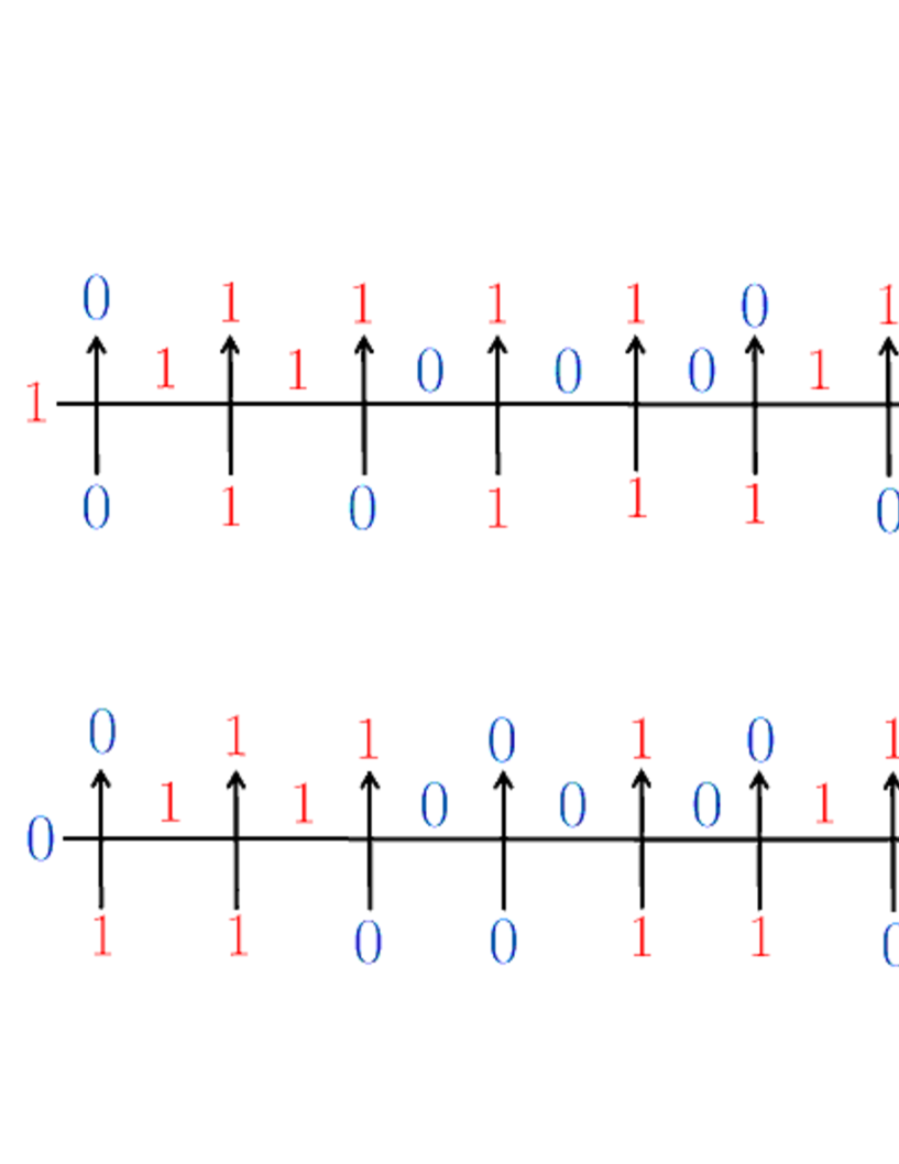
Figure 12: Graphical representations of the matrix elements $\langle 2,3,4,5,7,8,10|B(u)|2,4,5,6,8,10\rangle$ (top) and $\langle 2,3,5,7,8|C(u)|1,2,5,6,8,10\rangle$ (bottom). One can calculate from the above graphical description that $\langle 2,3,4,5,7,8,10|B(u)|2,4,5,6,8,10\rangle=(eu+f)\times(eu+ft)\times(1-t)cu\times(atu+b)\times(atu+b)\times(1-t)d\times(1-t)cu\times(atu+b)\times(au+b)\times(atu+b)=((1-t)cu)^{2}(1-t)d(atu+b)^{4}(au+b)(eu+tf)(eu+f)$.

Theorem 7.4.

We have the branching formula for the symmetric polynomials $G_{x}(u_{1},\dots,u_{N})$, $H_{\overline{x}}(u_{1},\dots,u_{N})$, $\overline{G}_{x}(u_{1},\dots,u_{N})$ and $\overline{H}_{\overline{x}}(u_{1},\dots,u_{N})$.

$$G_{y}(u_{1},\dots,u_{N},u_{N+1}) =\sum_{\begin{subarray}{c}x\\ y\succ x\end{subarray}}G_{y,x}(u_{N+1})G_{x}(u_{1},\dots,u_{N}),$$ (7.10)

$$H_{\overline{y}}(u_{1},\dots,u_{N},u_{N+1}) =\sum_{\begin{subarray}{c}\overline{x}\\ \overline{y}\succ\overline{x}\end{subarray}}H_{\overline{y},\overline{x}}(u_{N+1})H_{\overline{x}}(u_{1},\dots,u_{N}),$$ (7.11)

$$\overline{G}_{y}(u_{1},\dots,u_{N},u_{N+1}) =\sum_{\begin{subarray}{c}x\\ y\succ x\end{subarray}}\overline{G}_{y,x}(u_{N+1})\overline{G}_{x}(u_{1},\dots,u_{N}),$$ (7.12)

$$\overline{H}_{\overline{y}}(u_{1},\dots,u_{N},u_{N+1}) =\sum_{\begin{subarray}{c}\overline{x}\\ \overline{y}\succ\overline{x}\end{subarray}}\overline{H}_{\overline{y},\overline{x}}(u_{N+1})\overline{H}_{\overline{x}}(u_{1},\dots,u_{N}).$$ (7.13)

Proof.

We show (7.10). We use the argument in [8] which was used for the case of the Grothendieck polynomials. This follows by using (3.26) and (7.5) to calculate the action of ($N+1$) $B$-operators on the vacuum state $|\Omega\rangle$ as

$$\prod_{j=1}^{N+1}B(u_{j})|\Omega\rangle =B(u_{N+1})\prod_{j=1}^{N}B(u_{j})|\Omega\rangle$$

$$=B(u_{N+1})\sum_{x}G_{x}(u_{1},\dots,u_{N})|x_{1}\cdots x_{N}\rangle$$

$$=\sum_{y\succ x}G_{y,x}(u_{N+1})G_{x}(u_{1},\dots,u_{N})|y_{1}\cdots y_{N+1}\rangle,$$ (7.14)

on one hand, and comparing it with the direct evaluation

$$\prod_{j=1}^{N+1}B(u_{j})|\Omega\rangle=\sum_{y}G_{y}(u_{1},\dots,u_{N+1})|y_{1}\cdots y_{N+1}\rangle.$$ (7.15)

Equating the coefficients of the vectors $|y_{1}\cdots y_{N+1}\rangle$ in the right hand sides of (7.14) and (7.11) gives the branching formula (7.10). The other branching formulas (7.11), (7.12) and (7.13) van be proved in the same way. ∎

8 Conclusion

In this paper, we studied the combinatorial properties of certain classes of symmetric polynomials from the viewpoint of integrable lattice models in finite lattice. We introduced an integrable six-vertex model whose $L$-operator is the most general form intertwined by the $U_{q}(sl_{2})$ $R$-matrix, and analyzed the correspondence between the wavefunctions and the symmetric polynomials. The symmetric polynomials can be regarded as a generalization of the Grothendieck polynomials since taking the quantum group parameter to zero, the symmetric polynomials reduce to the Grothendieck polynomials. We proved the correspondence by combining the matrix product method and an expression for the homogeneous domain wall boundary partititon function. We remark that similar results for (3.26) in Theorem 3.2 have been obtained for the case of $q$-boson models [8, 20, 22, 24, 25, 26, 31] with fewer free parameters (except the inhomogeneous parameters) than the vertex model treated in this paper. It is interesting to find the corresponding $q$-boson model which is the counterpart of the spin-1/2 vertex model in this paper. A special case of the correspondence between the wavefunctions of the boson model and the spin-1/2 vertex model is given in [8].

Based on the correspondence, we examined several combinatorial properties of the symmetric polynomials. By taking the homogeneous limit of the Izergin-Korepin determinant form of the domain wall boundary partition functions, we extracted determinant pairing formulas for the symmetric polynomials introduced in this paper. The domain wall boundary partition function was used in the enumeration of the alternating sign matrices by taking limits of both the spectral and inhomogeneous parameters [47, 48, 49]. In this paper, we use the domain wall boundary partition function to extract pairing formulas between the symmetric polynomials. We just take the limit of the inhomogeneous paramaters and keeping the spectral parameters as they are.

By computing the matrix elements of the $B$- and $C$-operators explicitly, we also derived branching formulas for the symmetric polynomials. This is a direct consequence of the correpondence between the wavefunctions and the symmetric polynomials.

The combinatorial properties investigated in this paper holds for any value of the quantum group parameter $t$. By restricting the quantum group parameter to $t=0$ or $t=-1$, one can prove more combinatorial identities [7, 16] such as the Cauchy identity for the Grothendieck polynomials. It is interesting to find more combinatorial and algebraic identities by using the quantum inverse scattering method for the case either $t$ generic or by restricting to special values of $t$, when $t$ are roots of unity for example.

It is interesting to apply the analysis done in this paper to other models and other boundary conditions. One typical example is the reflecting boundary condition. The emerging symmetric polynomials change from the Schur polynomials to the symplectic Schur polynomials, or from the Hall-Littlewood polynomials to the $BC$-type versions for some integrable vertex and boson models [31, 34, 35, 36]. It is natural to expect that such kind of changes will also occur for the case of the integrable model treated in this paper.

References

[1]
H. Bethe,
Zur theorie der metalle: I. Eigenwerte und eigenfunktionen der linearen atomkette,
Z. Phys. 71, 205 (1931).
[3]
V. Drinfeld,
Hopf algebras and the quantum Yang-Baxter equation,
Sov. Math.-Dokl. 32, 254 (1985).
[4]
M. Jimbo,
A difference analog of and the Yang-Baxter equation,
Lett. Math. Phys. 10, 63 (1985).
[5]
L.D. Faddeev, E.K. Sklyanin, and L.A. Takhtajan,
Quantum inverse problem method. I,
Theor. Math. Phys. 40, 194 (1979).
[6]
V.E. Korepin, N.M. Bogoliubov and A.G. Izergin,
Quantum Inverse Scattering Method and Correlation functions,
(Cambridge University Press, Cambridge, 1993).
[7]
K. Motegi and K. Sakai,
Vertex models, TASEP and Grothendieck polynomials,
J. Phys. A: Math. Theor. 46, 355201 (2013).
[8]
K. Motegi, K. and Sakai,
-theoretic boson-fermion correspondence and melting crystals,
J. Phys. A: Math. Theor. 47, 445202 (2014).
[9]
A. Lascoux, and M. Schützenberger,
Structure de Hopf de
l’anneau de cohomologie et de l’anneau de Grothendieck d’une variété de
drapeaux,
C. R. Acad. Sci. Parix Sér. I Math
295, 629 (1982).
[10]
S. Fomin, and A.N. Kirillov,
Grothendieck polynomials and the Yang-Baxter equation,
Proc. 6th Internat. Conf. on Formal Power Series and
Algebraic Combinatorics, DIMACS 183-190 (1994).
[11]
A.S. Buch,
A Littlewood-Richardson rule for the K-theory of Grassmannians,
Acta. Math. 189, 37 (2002).
[12]
T. Ikeda, and H. Naruse,
-theoretic analogues of factorial Schur P-and Q-functions,
Adv. in Math. 243, 22 (2013).
[13]
T. Ikeda, and T. Shimazaki,
A proof of K-theoretic Littlewood-Richardson rules by Bender-Knuth-type involutions,
Math. Res. Lett. 21, 333 (2014).
[15]
A.N. Kirillov,
Notes on Schubert, Grothendieck and Key Polynomials,
SIGMA 12, 034 (2016).
[16]
K. Motegi, and K. Sakai,
Quantum integrable combinatorics of Schur polynomials,
arXiv:1507.06740.
[17]
B. Brubaker, D. Bump, and S. Friedberg,
Schur Polynomials and The Yang-Baxter Equation,
Commun. Math. Phys. 308, 281 (2011).
[18]
D. Bump, P. McNamara, and M. Nakasuji,
Factorial Schur functions and the Yang-Baxter equation,
Comm. Math. Univ. St. Pauli 63, 23 (2014).
[19]
K. Motegi,
Dual wavefunction of the Felderhof model,
arXiv:1606.08552.
[20]
N.M. Bogoliubov,
Boxed plane partitions as an exactly solvable boson model,
J. Phys. A 38, 9415 (2005).
[21]
K. Shigechi, and M. Uchiyama,
Boxed skew plane partition and integrable phase model,
J. Phys. A 38, 10287 (2005).
[22]
N.V. Tsilevich,
Quantum Inverse Scattering Method for the
-Boson Model and Symmetric Functions,
Funct. Anal. Appl. 40, 53 (2006).
[23]
C. Korff, and C. Stroppel,
The -WZNW Fusion Ring: a combinatorial construction and a realisation as quotient of quantum cohomology,
Adv. in Math. 225, 200 (2010).
[24]
A. Borodin,
On a family of symmetric rational functions,
arXiv:1410.0976.
[25]
A. Borodin, and L. Petrov,
Higher spin six vertex model and symmetric rational functions,
arXiv:1601.05770.
[26]
A. Borodin, and L. Petrov,
Lectures on Integrable probability:
Stochastic vertex models and symmetric functions,
arXiv:1605.01349.
[27]
V. Gorbounov and C. Korff,
Equivariant quantum cohomology and Yang-Baxter algebras,
arXiv:1402.2907.
[28]
V. Gorbounov, and C. Korff,
Quantum integrability and generalised quantum Schubert calculus,
arXiv:1408.4718.
[29]
D. Betea, M. Wheeler, and P. Zinn-Justin,
Refined Cauchy/Littlewood identities and six-vertex model partition functions: II. Proofs and new conjectures,
J. Alg. Comb. 42, 555 (2015).
[30]
D. Betea, and M. Wheeler,
Refined Cauchy and Littlewood identities, plane partitions and symmetry classes of alternating sign matrices,
J. Comb. Th. Ser. A 137, 126 (2016).
[31]
M. Wheeler and P. Zinn-Justin,
Refined Cauchy/Littlewood identities and six-vertex model partition functions: III. Deformed bosons,
Adv. in Math. 299, 543 (2016).
[32]
A. Duval, and V. Pasquier,
-bosons, Toda lattice, Pieri rules and Baxter -operator,
J. Phys. A:Math. Theor. 49, 154006 (2016).
[33]
K. Motegi, K. Sakai, and S. Watanabe,
Partition functions of integrable lattice models and combinatorics of symmetric polynomials,
arXiv:1512.07955.
[34]
J.F. van Diejen and E. Emsiz,
Orthogonality of Bethe Ansatz eigenfunctions for the Laplacian on a hyperoctahedral Weyl alcove,
Commun. Math. Phys. (2016).
[35]
D. Ivanov,
Symplectic Ice, in
Multiple Dirichlet series, L-functions
and automorphic forms, vol 300 of Progr. Math. Birkhäuser/Springer,
New York, 205-222 (2012).
[36]
B. Brubaker, D. Bump, G. Chinta, and P.E. Gunnells,
Metaplectic Whittaker Functions and Crystals of Type B., in
Multiple Dirichlet series, L-functions
and automorphic forms, vol 300 of Progr. Math. Birkhäuser/Springer,
New York, 93-118 (2012).
[37]
S.J. Tabony,
Deformations of characters, metaplectic Whittaker functions
and the Yang-Baxter equation, PhD. Thesis,
Massachusetts Institute of Technology, USA (2011).
[38]
A.M. Hamel, and R.C. King,
Tokuyama’s identity for factorial Schur and functions,
Elect. J. Comb. 22, 2 (2015).
[39]
Y. Takeyama
A discrete analogue of periodic delta Bose gas and affine Hecke algebra,
Funckeilaj Ekvacioj 57, 107 (2014).
[40]
Y. Takeyama,
A deformation of affine Hecke algebra and
integrable stochastic particle system,
J. Phys. A: Math. Theor. 47, 465203 (2014).
[41]
O. Golinelli, and K. Mallick,
Derivation of a Matrix Product Representation for the Asymmetric Exclusion Process from Algebraic Bethe Ansatz,
J. Phys. A:Math. Gen. 39, 10647 (2006).
[42]
H. Katsura, and I. Maruyama,
Derivation of Matrix Product Ansatz for the Heisenberg Chain from Algebraic Bethe Ansatz,
J. Phys. A:Math. Theor. 43, 175003 (2010).
[43]
V.E. Korepin,
Calculation of Norms of Bethe Wave Functions,
Commun. Math. Phys. 86, 391 (1982).
[44]
A. Izergin,
Partition function of the six-vertex model in a finite volume,
Sov. Phys. Dokl. 32, 878 (1987).
[45]
S. Pakuliak, V. Rubtsov, and A. Silantyev,
SOS model partition function and the elliptic weight functions,
J. Phys. A:Math. Theor. 41, 295204 (2008).
[46]
A.G. Izergin, D.A. Coker, and V.E. Korepin,
Determinant formula for the six-vertex model,
J. Phys. A 25, 4315 (1992).
[47]
D. Bressoud, Proofs and confirmations:
The story of the alternating sign matrix conjecture,
(MAA Spectrum, Mathematical Association of America,
Washington, DC, 1999).
[48]
G. Kuperberg,
Another proof of the alternating-sign matrix conjecture,
Int. Math. Res. Not. 3, 139 (1996).
[49]
G. Kuperberg,
Symmetry classes of alternating-sign matrices under one roof,
Ann. Math. 156, 835 (2002).