Reference Governor Strategies for Vehicle Rollover Avoidance

Abstract

The paper addresses the problem of vehicle rollover avoidance using reference governors applied to modify the driver steering input in vehicles with an active steering system. Several reference governor designs are presented and tested with a detailed nonlinear simulation model. The vehicle dynamics are highly nonlinear for large steering angles, including the conditions where the vehicle approaches a rollover onset, which necessitates reference governor design changes. Simulation results show that reference governor designs are effective in avoiding rollover. The results also demonstrate that the controllers are not overly conservative, adjusting the driver steering input only for very high steering angles.

Acronyms

AOA

Angle-of-Attack

AR

Aspect Ratio

AUV

Autonomous Underwater Vehicle

ASV

Autonomous Surface Vehicle

APF

Adaptive Particle Filter

AWA

Apparent Wind Angle

AWS

Apparent Wind Speed

BWA

B?? Wind Angle

CAS

Collision Avoidance System

CG

Command Governor

CM

Center of Mass

cdf

cumulative distribution function

CPCAA

Close Proximity Collision Avoidance Algorithm

CWA

C?? Wind Angle

DPG

Deconflicting Path Generator

DOF

Degrees-of-Freedom

ECG

Extended Command Governor

EKF

Extended Kalman Filter

ERG

Extended Reference Governor

ESC

Electronic Stability Control

ESP

Electronic Stability Program

FCS

Flight Control System

FOL

First-Order Logic

FRC

Foil Rotation Center

GNSS

Global Navigation Satellite System

GP

Gaussian process

GPS

Global Positioning System

GUI

Graphical User Interface

HCS

Hybrid Control System

HIL

Hardware-in-the-Loop

IID

Independent and Identically Distributed

IC

Internal Combustion

IMU

Inertial Measurement Unit

KF

Kalman Filter

LQR

Linear-Quadratic Regulator

LRG

Linear Reference Governor

LTR

Load Transfer Ratio

LWS

Layer Wind Shear

MWA

Mark Wind Angle

MPC

Model Predictive Controller

MPL

Multi-Point Linearization

NM

nautical miles

NHTSA

National Highway Traffic Safety Administration

NRG

Nonlinear Reference Governor

PDA

Path Deconflicting Algorithm

P

Proportional

PD

Proportional Derivative

PI

Proportional Integrative

PID

Proportional Integrative Derivative

pdf

probability density function

PL

Propositional Logic

PF

Particle Filter

QP

Quadratic Programming

RAPF

Regularized Adaptive Particle Filter

RG

Reference Governor

RHC

Receding Horizon Control

RPF

Regularized Particle Filter

RPM

Rotations Per Minute

SCG

Scalar Command Governor

SIL

Software-in-the-Loop

SMC

Sliding Mode Control

SWS

Surface Wind Shear

TCAS

Traffic Alert and Collision Avoidance System

TL

Temporal Logic

TWA

True Wind Angle

TWS

True Wind Speed

UAV

Unmanned Aerial Vehicle

UAS

Unmanned Aircraft System

UI

User Interface

VMG

Velocity Made Good

VMM

Velocity to the Mark

VPP

Velocity Prediction Program

VSC

Vehicle Stability Control

VTOL

Vertical Takeoff and Landing

WIP

Work in Progress

ZOH

Zero Order Hold

I Introduction

Rollover is an event where a vehicle’s roll angle increases abnormally. In most cases, this results from a loss of control of the vehicle by its driver.

This work focuses on the design of a supervisory controller that intervenes to avoid such extreme cases of loss of control. Conversely, in operating conditions considered normal the controller should not intervene, letting the driver commands pass through unaltered.

I-A Problem Statement

This paper treats the following problem for a vehicle equipped with an active front steering system. Given vehicle dynamics, a control model, and a set of predefined rollover avoidance constraints, find a control law for the steering angle such that the defined constraints are always enforced and the applied steering is as close as possible to that requested by the vehicle’s driver.

I-B Motivation

Between 1991 and 2001 there was an increase in the number of vehicle rollover fatalities when compared to fatalities from general motor vehicle crashes [1]. This has triggered the development of safety test standards and vehicle dynamics control algorithms to decrease vehicle rollover propensity. Rollover remains one of the major vehicle design and control considerations, in particular, for larger vehicles such as SUVs.

I-C Background and Notation

A variety of technologies, including differential braking, active steering, active differentials, active suspension and many others, are already in use or have been proposed to assist the driver in maintaining control of a vehicle. Since the introduction of the Electronic Stability Program (ESP) [2], much research has been undertaken on the use of active steering, see e.g., [3], to further enhance vehicle driving dynamics. According to [4] and [5], there is a need to develop driver assistance technologies that are transparent to the driver during normal driving conditions, but would act when needed to recover handling of the vehicle during extreme maneuvers. The active steering system has been introduced in production by ZF and BMW in 2003 [6].

For the rollover protection problem, Solmaz et al. [7, 8, 5] develop robust controllers which reduce the Load Transfer Ratio’s magnitude excursions. The presented controllers are effective at keeping the Load Transfer Ratio (LTR) within the desired constraints. Their potential drawbacks are that the controller is always active, interfering with the nominal steering input, or is governed by an ad hoc activation method. Furthermore, the controllers were tested with a linear model, whose dynamics may differ significantly from more realistic nonlinear models, in particular for larger steering angles, at which rollover is probable.

Constrained control methods have evolved significantly in recent years to a stage where they can be applied to vehicle control to enforce pointwise-in-time constraints on vehicle variables, thereby assisting the driver in maintaining control of the vehicle. Reference [9] is an indication of this trend.

We employ mostly standard notations throughout. We use $\left[a,b\right]$ to denote an interval (subset of real numbers between $a$ and $b$) for either $a<b$ or $a>b$.

I-D Original Contributions

This paper illustrates the development and the application of reference and extended command governors to LTR constraint enforcement and vehicle rollover avoidance. The reference governor (see [10] and references therein) is a predictive control scheme that supervises and modifies commands to well-designed closed-loop systems to protect against constraint violation. In the paper, we consider the application of both linear and nonlinear reference governor design techniques to vehicle rollover protection. While in the sequel we refer to the reference governors modifying the driver steering input, we note that they can be applied to modify the nominal steering angle generated by another nominal steering controller.

Our linear reference governor design exploits a family of linearizations of the nonlinear vehicle model for different steering angles. The linearized models are used to predict the vehicle response and to determine admissible steering angles that do not lead to constraint violation. In an earlier conference paper [11], reference and extended command governor designs for steering angle modification were proposed and validated on a linear vehicle model. This paper is distinguished by extending the design methodology to include compensation for nonlinear behavior, and validating the design on a comprehensive nonlinear vehicle model that includes nonlinear tire, steering, braking and suspension effects. The strong nonlinearity of the vehicle dynamics for high steering angles, the conditions where the vehicle is at risk of rolling over, caused the simpler controller presented in [11] to produce steering commands that were too conservative. The Linear Reference Governor (LRG) and Extended Command Governor (ECG) presented in Section III-G compensate for the strong nonlinearities with low interference over the driver input, while maintaining a low computational burden and a high effectiveness in avoiding car wheel lift.

For comparison, a Nonlinear Reference Governor (NRG) is also developed, which uses a nonlinear vehicle model for prediction of constraint violation and for the onboard optimization. This online reference governor approach is more computationally demanding but is able to take into account nonlinear model characteristics in the prediction.

The original contributions of this work are summarized as follows:

1. This paper demonstrates how Reference and Extended Command Governors [10], both linear and nonlinear, can improve the output adherence to the driver reference, while maintaining the vehicle within the desired constraints.

2. Conservatism, effectiveness, and turning response metrics are defined to evaluate, respectively, the controller command adherence to the driver reference, the constraints enforcement success, and the adherence of the vehicle trajectory in the horizontal plane to that desired by the driver.

3. Several methodological extensions to reference governor techniques are developed that can be useful in other applications.

I-E Paper Structure

The paper is organized as follows. Section II describes the vehicle models as well as the control constraints and the performance metrics used to evaluate the vehicle dynamic response under different designs. Section III-G describes reference governors considered in this paper, and includes preliminary performance evaluation to support the controller design decisions. Section IV illustrates the simulation results obtained with the different Reference Governors and comments on their comparative performance. Section V describes the conclusions of the current work, the current complementary research, and the follow-up work envisioned.

II Vehicle and Constraint Modeling

II-A Nonlinear Car Model

The nonlinear vehicle dynamics model is developed following [12, 5, 13, 14]. The model includes a nonlinear model for the tires’ friction and the suspension. The suspension model includes parameters to allow the simulation of a differential active suspension system.

II-A1 Vehicle Body Equations of Motion

Assuming that the sprung mass rotates about the Center of Mass (CM) of the undercarriage, that the car inertia matrix is diagonal, and that all the car wheels touch the ground, the car nonlinear model is defined by:

$$F_{x,T} =m\left(\dot{u}-vr\right)+m_{SM}h_{SM}p\cos\phi,$$ (1a)

$$F_{y,T} =m\left(\dot{v}+ur\right)-m_{SM}h_{SM}\left(\dot{p}\cos\phi-p^{2}\sin\phi\right),$$ (1b)

$$L_{T} =-K_{s}\left(1-\overline{\Delta k}_{ss}^{2}\right)\tan\phi-$$

$$D_{s}\left(1-\overline{\Delta d}_{ss}^{2}\right)p\cos\phi-mg\left(\overline{\Delta k}_{ss}+\overline{\Delta d}_{ss}\right),$$ (1c)

$$N_{T} =I_{zz}\dot{r},$$ (1d)

$$\dot{p} =\frac{h_{SM}m_{SM}\left(\frac{F_{y,T}}{m}+\sin\phi\left(g+h_{SM}\frac{m_{UC}}{m}p^{2}\right)\right)+L_{T}}{I_{xx,SM}+h^{2}_{SM}m_{SM}\frac{m_{UC}}{m}\cos\phi}.$$

Most of the model parameters are illustrated in Figure 1 and their values are given in Table II for the simulation model used. The model states are the vehicle velocity components in the horizontal plane ($u,v$), roll ($\phi$), roll rate ($p$), and turn rate ($r$). $F_{x,T}$, $F_{y,T}$, $L_{T}$, and $N_{T}$ are the forces and moments acting on the car through the tires. $m_{SM}$, $m_{UC}$, $m$, $I_{xx,SM}$ and $I_{zz}$ are the sprung mass, the undercarriage, and the overall vehicle mass and inertia moments, respectively. $K_{s}$ and $D_{s}$ are the suspension roll stiffness and damping coefficients, and $\overline{\Delta k}_{ss}$ and $\overline{\Delta d}_{ss}$ are the suspension roll differential stiffness and damping factors.

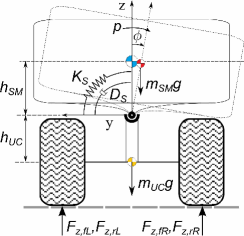
(a) Rear view.

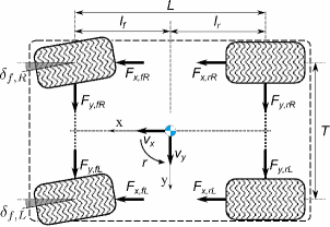
(b) Top view.

Figure 1: Vehicle forces diagram.

The simulation results (sec. IV) include some instants where the wheels on one of the sides lift from the road. In such conditions, the car dynamics are similar to a two segment inverted pendulum [15]. For the sake of readability and because it is not relevant for the design of the reference governors that maintain vehicle operation away from this condition, the extension of the vehicle equations of motion for the wheel lift condition is not presented here.

II-A2 Magic Formula Tire Model

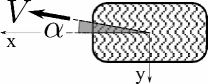
Figure 2: Tire slip angle ($\alpha$) at the contact patch. $V$ is the total tire speed.

The main source of nonlinearities in the equations of motion is the tire forces’ dependence on slip. In this work, we use the Magic Formula tire model [16, 13, 17, 18]. To compute the tire forces, the slip ratio ($\lambda$) and the tire slip angle ($\alpha$) are defined as (fig. 2):

$$\lambda =\begin{cases}\frac{R_{w}\omega_{w}-u_{w}}{u_{w}}&R_{w}\omega_{w}<u_{w}\\ \frac{R_{w}\omega_{w}-u_{w}}{R_{w}\omega_{w}}&R_{w}\omega_{w}\geq u_{w}\end{cases},$$ (2a)

$$\alpha_{f} =\delta_{f}-\tan^{-1}\frac{v+l_{f}r}{u},$$ (2b)

$$\alpha_{r} =\tan^{-1}\frac{-v+l_{r}r}{u}.$$ (2c)

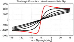
Figure 3: Tire lateral force variation with the side slip for several levels of slip ratio.

The tire slip ratio ($\lambda$) characterizes the longitudinal slip. It is defined as the normalized difference between wheel hub speed ($u_{w}$) and wheel circumferential speed ($R_{w}\omega_{w}$). The tire slip angle ($\alpha$) is the angle between the tire heading direction and the velocity vector at the contact patch (fig. 2). Equations (2b) and (2c) define the tire slip angle for the forward and rear wheels, respectively. For combined longitudinal and lateral slip, the Magic Formula takes the following form [12] (fig. 3):

$$\left[\begin{array}[]{c}F_{x}^{T}\\ F_{y}^{T}\end{array}\right] =F_{P}P\left(s_{c},C,E\right)\hat{\mathbf{s}},$$ (5)

$$P\left(s_{c},C,E\right) =\sin\left(C\tan^{-1}\left[\frac{s_{c}}{C}\left(1-E\right)+E\tan^{-1}\left(\frac{s_{c}}{C}\right)\right]\right),$$

$$s_{c} =\frac{C_{\alpha}\left\|\mathbf{s}\right\|}{F_{p}},\>\>\>C_{\alpha}=c_{1}mg\left(1-e^{-\frac{c_{2}F_{z}}{mg}}\right),$$

$$c_{1} =\frac{BCD}{4\left(1-e^{-\frac{c_{2}}{4}}\right)},$$

$$F_{P} =\frac{F_{z}1.0527D}{1+\left(\frac{1.5F_{z}}{mg}\right)^{3}},$$

$$\mathbf{s} =\left[\begin{array}[]{c}s_{x}\\ s_{y}\end{array}\right]=\left[\begin{array}[]{c}\lambda\\ \tan\alpha\end{array}\right],\>\>\>\hat{\mathbf{s}}=\frac{\mathbf{s}}{\left\|\mathbf{s}\right\|},$$ (10)

where $F_{x}^{T}$ and $F_{y}^{T}$ are the forces along the tire longitudinal and lateral axis, $x$ and $y$ (fig. 2), respectively. $C_{\alpha}$ is the cornering stiffness, $F_{P}$ is the horizontal (or slip) peak force, $\hat{\mathbf{s}}$ is the total slip, and $B$, $C$, $D$, $E$, and $c_{2}$ are tire parameters that depend on the tire characteristics and the road conditions (see Table I).

TABLE I: Tires Magic Formula model parameters.

Conditions	$B$	$C$	$D$	$E$	$c_{2}$
Dry	$7.15$	$2.30$	$0.87$	$1.00$	$1.54$
Wet	$9.00$	$2.50$	$0.72$	$1.00$	$1.54$
Snow	$5.00$	$2.00$	$0.30$	$1.00$	$1.54$
Ice	$4.00$	$2.00$	$0.10$	$1.00$	$1.54$

Figure 4 illustrates the variation of the lateral force with the vertical load. The illustrated model presents almost the same side slip angle for all vertical load cases, and an initial slope decreasing for lower vertical loads. This behavior is governed by the parameter $c_{2}$.

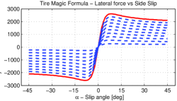
Figure 4: Tire lateral force variation with the vertical load. The solid red line is the lateral force generated at nominal vertical load.

II-B Constraints

The vehicle constraints reflect the system’s physical limits or requirements to keep the vehicle state in a safe region. There are several options to define constraints that protect the vehicle from rollover. One possibility is to define the rollover constraints as the states where the car roll is so large that there is no possible recovery. This approach would require the treatment of complex, hybrid vehicle dynamics, which involve the vehicle continuous dynamics states plus two discrete states (all wheels on the road state and wheel liftoff state), and in the case of wheel liftoff, multiple-body inverted pendulum-like dynamics.

In this paper, following also [7, 8, 5], more conservative rollover avoidance constraints are treated, which are, however, simpler to enforce. These constraints are defined through the Load Transfer Ratio (LTR). The LTR measures how much of the vehicle vertical load is concentrated on one of the vehicle sides:

$$LTR:=\frac{F_{z,R}-F_{z,L}}{mg}.$$ (11)

The wheel liftoff happens when the LTR increases above $1$ or decreases below $-1$, i.e., when the right or left wheels, respectively, bear all the car’s weight. Hence, the rollover avoidance constraints are imposed as:

$$LTR\in\left[-LTR_{lim},LTR_{lim}\right],\>\>0<LTR_{lim}<1.$$ (12)

Remark 1.

Note that the absolute value of the LTR may exceed 1, even if wheel liftoff does not occur. This can happen, in particular, due to the suspension roll moment, e.g., generated by the spring stored energy, and by the CM vertical acceleration during wheel liftoff.

The steering input is also considered to be constrained:

$$\delta_{SW}\in\left[-\delta_{SW,lim},\delta_{SW,lim}\right].$$ (13)

II-C Linearized Car Model

The vehicle linear model has the following form,

$$\dot{\mathbf{x}} =\mathbf{A}\mathbf{x}+\mathbf{B}_{\delta_{S}}k_{\delta_{SW}}\Delta\delta_{SW},$$ (14a)

$$\mathbf{y} =\mathbf{C}\mathbf{x}+\mathbf{D}_{\delta_{SW}}\Delta\delta_{SW},$$ (14b)

where $\mathbf{x}=\left[\Delta v,\Delta p,\Delta r,\Delta\phi\right]$ correspond to the relevant lateral state variables. $\Delta\delta_{SW}$ is the steering control input deviation. The ratio between the steering wheel angle and the forward tires steering angles is $k_{\delta_{SW}}$.

Linearizing (1), the vehicle linearized model is obtained, with the dynamics matrix of the form,

$$\mathbf{A}:=\left[\begin{array}[]{cccc}\frac{\partial F_{y,T}}{\partial v}\frac{1}{m^{\prime}}&\frac{\partial F_{y,T}}{\partial r}\frac{1}{m^{\prime}}-u&h^{\prime}_{SM}\frac{\partial\dot{p}}{\partial p}&h^{\prime}_{SM}\frac{\partial\dot{p}}{\partial\phi}\\ \frac{\partial N_{T}}{\partial v}\frac{1}{I_{zz}}&\frac{\partial N_{T}}{\partial r}\frac{1}{I_{zz}}&0&0\\ \frac{\partial F_{y,T}}{\partial v}\frac{h_{SM}}{I^{\prime}_{xx}}&\frac{\partial F_{y,T}}{\partial r}\frac{h_{SM}}{I^{\prime}_{xx}}&\frac{\partial\dot{p}}{\partial p}&\frac{\partial\dot{p}}{\partial\phi}\\ 0&0&1&0\end{array}\right],$$ (15)

where

$$m^{\prime} =\frac{m^{2}I^{\prime}_{xx}}{mI^{\prime}_{xx}+h^{2}_{SM}m^{2}_{SM}\cos\phi_{0}},$$ (16a)

$$I^{\prime}_{xx} =I_{xx,SM}+h^{2}_{SM}m_{SM}\frac{m_{UC}}{m}\cos\phi,$$ (16b)

$$h^{\prime}_{SM} =\frac{h_{SM}m_{SM}}{m},$$ (16c)

$$\frac{\partial\dot{p}}{\partial p} =\frac{2h^{2}_{SM}m_{SM}p_{0}\frac{m_{UC}}{m}\sin\phi_{0}-D_{s}\left(1-\overline{\Delta d}_{ss,0}^{2}\right)\cos\phi_{0}}{I^{\prime}_{xx}},$$ (16d)

$$\frac{\partial\dot{p}}{\partial\phi} =\left[m_{SM}gh_{SM}-K_{s}\left(1-\overline{\Delta k}_{ss,0}^{2}\right)\left(1+\tan^{2}\phi_{0}\right)-\right.$$

$$\left.D_{s}\left(1-\overline{\Delta d}_{ss,0}^{2}\right)p_{0}\sin\phi_{0}\right]/I^{\prime}_{xx}.$$ (16e)

The steering control matrix is defined as:

$$\mathbf{B}_{\delta_{S}}:=\left[\begin{array}[]{cccc}\frac{\partial F_{y,T}}{\partial\delta_{f}}\frac{1}{m^{\prime}}&\frac{\partial N_{T}}{\partial\delta_{f}}\frac{1}{I_{zz}}&\frac{\partial F_{y,T}}{\partial\delta_{f}}\frac{h_{SM}}{I^{\prime}_{xx}}&0\end{array}\right]^{\intercal},$$ (17)

The system output matrices are defined by the operation constraints (sec. II-B):

$$\mathbf{C} :=\left[\begin{array}[]{cccc}0&0&\frac{2D_{s}}{mgT}&\frac{2K_{s}}{mgT}\\ 0&0&0&0\end{array}\right],$$ (18c)

$$\mathbf{D}_{\delta_{S}} :=\left[\begin{array}[]{ccccccc}0&1\end{array}\right]^{\intercal}.$$ (18e)

II-D Performance Metrics

This study uses four performance metrics: the step computation time, the effectiveness, the conservatism, and the turning response. We have chosen not to use a metric that compares the vehicle positions between the reference trajectory and the trajectory affected by the controllers as there are several reference trajectories that end in a full rollover.

The step computation time is the time it takes the controller to perform the constraint enforcement verification and compute a command. The effectiveness metric is the success rate in avoiding wheel lift up to a wheel lift limit. For each test:

$$\eta_{lift}:=1-\frac{\max z_{wheel}}{z_{wheel,lim}},$$ (19)

where $\max z_{wheel}$ is the maximum wheel lift attained during a test, and $z_{wheel,lim}$ is the wheel lift limit considered.

The conservatism metric indicates how much the controller is over-constraining the steering command when compared with a safe steering command:

$$\chi:=\frac{\int_{0}^{T}\left(\left|\delta_{SW,ref}-\delta_{SW}\right|-\left|\delta_{SW,ref}-\delta_{SW,safe}\right|\right)dt}{\int_{0}^{T}\left|\delta_{SW,ref}\right|dt},$$ (20)

where $\delta_{SW,ref}$ is the driver reference command during the maneuver, $\delta_{SW}$ is the controller command, $\delta_{SW,safe}$ is a reference safe command, and $T$ is the test duration. Two options for the reference safe command are the driver steering input scaled down to avoid any wheel lift or the driver steering input scaled down to produce a maximum wheel lift of $z_{wheel,lim}$.

The turning response metric indicates how much the controller is limiting the vehicle turn rate relative to the driver desired turning rate when compared with the turn rate achieved with a safe steering command:

$$\eta_{\psi}:=\frac{\int_{0}^{T}\left(\left|\psi_{des}-\psi_{safe}\right|-\left|\psi_{des}-\psi\right|\right)dt}{\int_{0}^{T}\left|\psi_{SW,ref}\right|dt},$$ (21)

where the driver desired turning rate is inferred from the reference steering command and the steering-to-turn rate stability derivative: $\psi_{des}=\left.\frac{d\psi}{d\delta_{SW}}\right|_{\delta_{SW}=0}\delta_{SW,ref}$. $\psi$ and $\psi_{safe}$ are the turn rates caused by the controller command and the reference safe command, respectively.

III Reference and Command Governors

This work implements different versions of Reference and Command Governor (CG) controllers, collectively referred to by their common name as reference governors. Our reference governors modify the reference command, the steering angle (fig 5), if this reference command is predicted to induce a violation of the LTR constraints (sec. II-B).

The reference governors solutions studied for this application are based on both linear and nonlinear models. The following sections describe the various solutions in more detail.

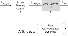
Figure 5: Command governor control architecture for a steering command.

III-A Linear Reference Governors and Command Governors

Both the Linear Reference Governors and the Command Governors rely on a maximum output admissible set $\mathcal{O}_{\infty}$ (or its subsets) to check if a reference command is safe, i.e., if it does not lead to constraint violation, and to compute a safe alternative command, if necessary. The $\mathcal{O}_{\infty}$ set characterizes the combinations of constant commands and vehicle states that do not lead to constraint violating responses,

$$\mathcal{O}_{\infty}:=\left\{\left(\mathbf{u},\mathbf{x}\right)|\mathbf{y}_{k}\in\mathbf{Y},\forall k\in\mathbb{Z}^{0+}\right\}\subset\mathbb{R}^{4+n},$$ (22)

where $n=1$ is the number of control variables, $\mathbf{x}$ and $\mathbf{u}$ are the state and command at the present moment and $\mathbf{y}_{k},k\in\mathbb{Z}^{0+}$, is the predicted evolution of the system output. The set $\mathbf{Y}$ represents the constraints and delineates safe outputs

$$\mathbf{Y}:=\left\{\mathbf{y}|\mathbf{A}_{y}\mathbf{y}\leq\mathbf{b}_{y}\right\}\subset\mathbb{R}^{l},$$ (23)

where $l$ is the number of system outputs on which constraints are imposed.

Considering (22), (23), $\mathbf{x}_{\mathcal{O}_{\infty}}:=\left[\begin{array}[]{ccc}\mathbf{u}&\mathbf{x}\end{array}\right]^{\intercal}$, and a linear model (14), we define an inner approximation of the maximum output admissible set as

$$\mathcal{O}_{\infty} :=\left\{\mathbf{x}_{\mathcal{O}_{\infty}}|\mathbf{A}_{\mathcal{O}_{\infty}}\mathbf{x}_{\mathcal{O}_{\infty}}\leq\mathbf{b}_{\mathcal{O}_{\infty}}\right\}\subset\mathbb{R}^{4+n},$$ (24a)

$$\mathbf{A}_{\mathcal{O}_{\infty}} :=\left[\begin{array}[]{cc}\mathbf{A}_{y}\mathbf{D}&\mathbf{A}_{y}\mathbf{C}\\ \mathbf{A}_{y}\left(\mathbf{C}\left(\mathbf{I}-\mathbf{A}\right)^{-1}\left(\mathbf{I}-\mathbf{A}\right)\mathbf{B}+\mathbf{D}\right)&\mathbf{A}_{y}\mathbf{C}\mathbf{A}\\ \vdots&\vdots\\ \mathbf{A}_{y}\left(\mathbf{C}\left(\mathbf{I}-\mathbf{A}\right)^{-1}\left(\mathbf{I}-\mathbf{A}^{N}\right)\mathbf{B}+\mathbf{D}\right)&\mathbf{A}_{y}\mathbf{C}\mathbf{A}^{N}\\ \mathbf{A}_{y}\mathbf{H}&0\end{array}\right],$$ (24g)

$$\mathbf{b}_{\mathcal{O}_{\infty}} :=\left[\begin{array}[]{c}\mathbf{b}_{y}\\ \mathbf{b}_{y}\\ \vdots\\ \mathbf{b}_{y}\\ \mathbf{b}_{y}\left(1-\epsilon\right)\end{array}\right],$$ (24m)

$$H =\mathbf{C}\left(\mathbf{I}-\mathbf{A}\right)^{-1}\mathbf{B}+\mathbf{D},$$ (24n)

where $N$ is the selected prediction horizon and $\epsilon>0$. Under mild assumptions [19], $\mathcal{O}_{\infty}$ is the same for all $N$ sufficiently large and is positively invariant (for constant $u$) and satisfies constraints pointwise. Generally, such an N is comparable to the settling time of the system.

III-B Linear Reference Governor (LRG)

The LRG computes a single command value on every update using the above $\mathcal{O}_{\infty}$ set which we re-write as

$$\mathcal{O}_{\infty} :=\left\{\left(\mathbf{u},\mathbf{x}\right)|\mathbf{y}_{k}=\left(\mathbf{C}\left(\mathbf{I}-\mathbf{A}\right)^{-1}\left(\mathbf{I}-\mathbf{A}^{k}\right)\mathbf{B}+\mathbf{D}\right)\mathbf{u}+\right.$$

$$\left.\mathbf{C}\mathbf{A}^{k}\mathbf{x}\in\mathbf{Y},k=0,...,N\right\}\bigcap\Gamma\subset\mathbb{R}^{4+n},$$ (25)

$$\Gamma =\left\{\left(\mathbf{u},\mathbf{x}\right)|\mathbf{H}\mathbf{u}\in\left(1-\epsilon\right)\mathbf{Y}\right\}.$$

By applying the $\mathcal{O}_{\infty}$ to the current state, the controller checks if the reference or an alternative command are safe. If the reference command is deemed safe, it is passed to the actuator. If not, the controller selects an alternative safe command that minimizes the difference to the reference:

$$\mathbf{v}_{k} =\arg\!\max_{\mathbf{v}_{k}}\left\{k_{RG}|\mathbf{v}_{k}=\mathbf{v}_{k-1}+k_{RG}\left(\mathbf{u}_{k}-\mathbf{v}_{k-1}\right),\right.$$

$$\left.\left(\mathbf{v}_{k},\mathbf{x}_{k}\right)\in\mathcal{O}_{\infty}\>\mathsf{and}\>k_{RG}\in\left[0,1\right]\right\},$$ (26)

where $\mathbf{u}_{k}$ is the current reference command, $\mathbf{x}_{k}$ is the current state, and $\mathbf{v}_{k-1}$ is the previous command used.

Remark 2.

Because the reference governor checks at each update if a command is safe for the future steps, $\mathbf{v}_{k-1}$ is assured to be safe for the current step, provided an accurate model of the system is used. As such, in the optimization process (26), one only needs to analyze the interval $\mathbf{u}\in\left[\mathbf{v}_{k-1},\mathbf{u}_{k}\right]$.

III-C Extended Command Governor (ECG)

The ECG [20] is similar to the LRG, but, when it detects an unsafe reference command, it computes a sequence of safe commands governed by:

$$\mathbf{v} =\bar{\mathbf{C}}\bar{\mathbf{x}}+\mathbf{\rho},$$ (27a)

$$\bar{\mathbf{x}}_{k+1} =\bar{\mathbf{A}}\bar{\mathbf{x}},$$ (27b)

where $\mathbf{v}$ is the safe command (output of the ECG) with dynamics governed by (27b), $\bar{\mathbf{x}}$ is the virtual state vector of the command dynamics, and $\mathbf{\rho}$ is the steady state command to which the sequence converges. The matrices $\bar{\mathbf{A}}$ and $\bar{\mathbf{C}}$ are two of the design elements of the ECG. They are defined at the end of this section. The key requirement is that the matrix $\bar{\mathbf{A}}$ must be Schur.

To detect if a reference command is safe, the ECG uses the LRG $\mathcal{O}_{\infty}$ set (III-B). If the reference command is unsafe, the ECG uses an augmented $\check{\mathcal{O}}_{\infty}$ set that takes into account the computed command dynamics:

$$\check{\mathcal{O}}_{\infty} :=\left\{\left(\mathbf{\rho},\mathbf{x}_{aug}\right)|\mathbf{y}_{k}=\right.$$

$$\left.\left(\mathbf{C}_{aug}\left(\mathbf{I}-\mathbf{A}_{aug}\right)^{-1}\left(\mathbf{I}-\mathbf{A}_{aug}^{k}\right)\mathbf{B}_{aug}+\mathbf{D}_{aug}\right)\mathbf{\rho}+\right.$$

$$\left.\mathbf{C}_{aug}\mathbf{A}_{aug}^{k}\mathbf{x}_{aug}\in\mathbf{Y},k=0,...,N\right\}\bigcap\Gamma^{\prime}\subset\mathbb{R}^{4+n+m},$$ (28)

$$\Gamma^{\prime} =\left\{\left(\mathbf{\rho},\mathbf{x}_{aug}\right)|\mathbf{H}\mathbf{\rho}\in\left(1-\epsilon\right)\mathbf{Y}\right\},$$

where $m$ is the size of $\bar{\mathbf{x}}$, $\mathbf{x}_{aug}^{\intercal}:=\left[\mathbf{x}^{\intercal},\bar{\mathbf{x}}^{\intercal}\right]^{\intercal}$ is an augmented state vector, and the matrices $A_{aug},B_{aug},C_{aug},D_{aug}$ correspond to the augmented system. We note that this event-triggered execution of ECG is quite effective in reducing average chronometric loading and to the authors’ knowledge, has not been previously proposed elsewhere.

In the ECG, both the steady state command and the initial virtual state are optimized. This optimization is performed by solving the following quadratic programming problem:

$$\mathbf{x}^{\prime} =\arg\!\min_{\mathbf{x}^{\prime}}\left\{\frac{1}{2}\mathbf{x}^{\prime\intercal}\mathbf{H}\mathbf{x}^{\prime}+\mathbf{f}\mathbf{\rho}|\left(\mathbf{\rho},\mathbf{x}_{aug}\right)\in\check{\mathcal{O}}_{\infty}\right\},$$ (29)

$$\mathbf{x}^{\prime} :=\left[\begin{array}[]{c}\bar{\mathbf{x}}\\ \rho\end{array}\right],\>\mathbf{H}:=\left[\begin{array}[]{cc}\mathbf{P}&0\\ 0&\mathbf{Q}\end{array}\right],\>\mathbf{f}:=-\mathbf{u}_{k}^{\intercal}\mathbf{Q},$$ (34)

where $\mathbf{P}$ and $\mathbf{Q}$ are symmetric positive-definite matrices. In this work $\mathbf{Q}:=k_{L}\mathbf{I}>0$ is the tuning matrix, while $\mathbf{P}$ is computed by solving the discrete-time Lyapunov equation:

$$\bar{\mathbf{A}}^{\intercal}\mathbf{P}\bar{\mathbf{A}}-\mathbf{P}+\mathbf{Q}=0.$$ (35)

The safe command is then computed by (27a).

Several possibilities for the matrices $\bar{\mathbf{A}}$ and $\bar{\mathbf{C}}$ exist [10]. These matrices can define a shift register sequence, making the ECG behave like a Model Predictive Controller (MPC), or a Laguerre sequence, as follows:

$$\bar{\mathbf{A}} =\left[\begin{array}[]{ccccc}\alpha\mathbf{I}_{m}&\mu\mathbf{I}_{m}&-\alpha\mu\mathbf{I}_{m}&\ldots&\left(-\alpha\right)^{N-2}\mu\mathbf{I}_{m}\\ 0&\alpha\mathbf{I}_{m}&\mu\mathbf{I}_{m}&\ldots&\left(-\alpha\right)^{N-3}\mu\mathbf{I}_{m}\\ 0&0&\alpha\mathbf{I}_{m}&\ddots&\vdots\\ 0&0&0&\ldots&\mu\mathbf{I}_{m}\\ 0&0&0&\ldots&\alpha\mathbf{I}_{m}\end{array}\right],$$ (36f)

$$\bar{\mathbf{C}} =\left[\begin{array}[]{ccccc}\mathbf{I}_{m}&-\alpha\mathbf{I}_{m}&\alpha^{2}\mathbf{I}_{m}&\ldots&\left(-\alpha\right)^{N-1}\mathbf{I}_{m}\end{array}\right],$$ (36h)

where $\mu=1-\alpha$ and $0\leq\alpha\leq 1$ is a tuning parameter that corresponds to the time constant of the command virtual dynamics. If $\alpha=0$, the ECG becomes a shift register.

III-D Steering Control

The output and the constraints of the RG are defined as follows:

$$\mathbf{y} :=\left[\begin{array}[]{cc}LTR&\delta_{SW}\end{array}\right]^{\intercal},$$ (37b)

$$\mathbf{A}_{y} :=\left[\begin{array}[]{cc}1&0\\ -1&0\\ 0&1\\ 0&-1\end{array}\right],\>\mathbf{b}_{y}:=\left[\begin{array}[]{c}LTR_{lim}\\ LTR_{lim}\\ \delta_{SW,lim}\\ \delta_{SW,lim}\end{array}\right].$$ (37k)

The discrete time step for the dynamics matrices is $\Delta t=0.01s$ and the prediction horizon is $N=100$. For the ECG, the optimization gain is $k_{L}=1$, the virtual state vector size is $4$, and the $\alpha=1-\frac{\Delta t}{\tau_{car}}$, so that the virtual dynamics match the vehicle dynamics time constant that, as we have determined empirically, appears to provide best response properties.

III-E Nonlinear Compensation

Both the Linear Reference Governor and the Extended Command Governor rely on linear model predictions to avoid breaching the defined constraints. In reality, the controller is acting on a vehicle with nonlinear dynamics. This results in deviations between the predicted and the real vehicle response.

III-E1 Nonlinear Difference

For the same state, there is a difference between the linear model output prediction and the vehicle’s real output variables, which we refer to as the nonlinear difference:

$$\mathbf{d}=f\left(\mathbf{x},\mathbf{u}\right)-\mathbf{C}\mathbf{x}-\mathbf{D}\mathbf{u}-\mathbf{y}_{0}.$$ (38)

This difference, further exacerbated by the error in the state prediction by the linear model, can either cause the vehicle to breach the constraints when the controller does not predict so, or cause the controller generated command to be too conservative. This effect can be mitigated if the controller takes into account the current nonlinear difference for the current command computation, assuming that it is persisting over the prediction horizon. As an example, the nonlinear difference can be compensated in the LRG by including it in the $\mathcal{O}_{\infty}$ set:

$$\check{\mathcal{O}}_{\infty} :=\left\{\left(\mathbf{v},\mathbf{x},\mathbf{d}\right):\mathbf{y}_{k}=\right.$$

$$\left.\left(\mathbf{C}\left(\mathbf{I}-\mathbf{A}\right)^{-1}\left(\mathbf{I}-\mathbf{A}^{k}\right)\mathbf{B}+\mathbf{D}\right)\mathbf{v}+\right.$$

$$\left.\mathbf{C}\mathbf{A}^{k}\mathbf{x}+\mathbf{d}\in\mathbf{Y},k=0,...,N\right\}\bigcap\Gamma^{\prime\prime}\subset\mathbb{R}^{4+n+l},$$ (39)

$$\Gamma^{\prime\prime} =\left\{\left(\mathbf{v},\mathbf{x},\mathbf{d}\right)|\mathbf{H}\mathbf{v}+\mathbf{d}\in\left(1-\epsilon\right)\mathbf{Y}\right\}.$$

To use the nonlinear difference in the controller, the $\mathbf{x}_{\mathcal{O}_{\infty}}$ vector and the $\mathbf{A}_{\mathcal{O}_{\infty}}$ matrix are extended to account for $\mathbf{d}$:

$$\breve{\mathbf{x}}_{\mathcal{O}_{\infty}}^{\intercal} :=\left[\begin{array}[]{ccc}\mathbf{u}^{\intercal},&\mathbf{x}^{\intercal},&\mathbf{d}^{\intercal}\end{array}\right]^{\intercal},$$ (40b)

$$\breve{\mathbf{A}}_{\mathcal{O}_{\infty}} :=\left[\begin{array}[]{cc}\mathbf{A}_{\mathcal{O}_{\infty}}&\begin{array}[]{cc}\mathbf{A}_{y}\\ \mathbf{A}_{y}\\ \vdots\\ \mathbf{A}_{y}\end{array}\end{array}\right],\>\breve{\mathbf{b}}_{\mathcal{O}_{\infty}}:=\mathbf{b}_{\mathcal{O}_{\infty}}.$$ (40h)

III-E2 Multi-Point Linearization (MPL)

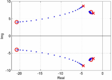
Figure 6: Vehicle dynamics’ poles for a range of steering angles from 0 degrees (cross) to 150 degrees (circle).

The nonlinear difference compensation in the previous subsection reduces the nonlinear effects in the vicinity of the system’s current state. However, in this work and in particular for large input commands, that are likely to cause a rollover, this alone is insufficient. Figure 6 shows how much the vehicle dynamics’ poles can change for a range of steering angles. If the controller uses a model linearized around the no actuation point ($\delta_{SW}=0$), the controller becomes too conservative. The use of multiple linearization points to define multiple $\mathcal{O}_{\infty}$ sets has proved to be an appropriate compensation. The multi-point linearization results in a less conservative controller, when compared to a controller just with the nonlinear difference compensation (fig. 7a).

The control strategy is the same as described in the previous sections. The difference is that several linearization points are selected (fig. 7b) and, for each one, an $\mathcal{O}_{\infty}$ set (24) is computed. The controller then selects the closest linearization point and corresponding $\mathcal{O}_{\infty}$ set, based on the current steering angle. Note that in Figure 7a and subsequent figures we report LTR in percent.

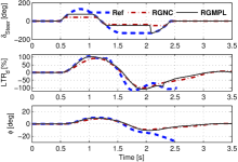
(a) Vehicle steering command, LTR response, and roll response. The dashed blue line is the reference command. The dot-and-dashed red and the solid black lines are the LRG commands with a single- and multi-point linearization, respectively, both with the nonlinear difference compensation.

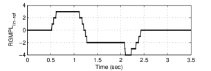
(b) Linearization point selection in the LRG with multi-point linearization.

Figure 7: LRG with multi-point linearization. Here linearization points used corresponded to steering angles of $\delta_{SW}=0,20,40,80\>\&\>130deg$.

III-F Command Computation Feasibility

In practical applications, the LRG and ECG optimization problems, (26) and (29), may become infeasible due to unmodeled uncertainties, in particular, due to the approximation of the nonlinear vehicle dynamics by a linear model in prediction. Figure 8a shows the computation feasibility classification for an example vehicle simulation. This section describes the different approaches to deal with infeasibility and the outcomes of their evaluation.

III-F1 Last Successful Command Sequence

The simplest approach, in the event of infeasibility, is to maintain the last successfully computed command, for the LRG:

$$\mathbf{v}_{k}=\mathbf{v}_{k-1},$$ (41)

or command sequence, for the ECG:

$$\bar{\mathbf{x}}_{k} =\bar{\mathbf{A}}\bar{\mathbf{x}}_{k-1},$$ (42a)

$$\mathbf{\rho}_{k} =\mathbf{\rho}_{k-1},$$ (42b)

$$\mathbf{v}_{k} =\bar{\mathbf{C}}\bar{\mathbf{x}}_{k}+\mathbf{\rho}_{k}.$$ (42c)

III-F2 Command Contraction

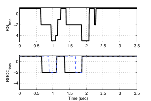
(a) Classification of the solution computation feasibility for the LRG. Level 1 means the controller is able to compute a solution. Level 0 means that there is no viable solution, because the current output is already breaching the constraints and the current reference is the same as the last used command. The levels $-1$ and $-2$ indicate that for some of the points in the prediction horizon a solution would only exist if the gain $k_{LRG}$ was set to more than $1$ or less than $0$, respectively. Level $-3$ indicates that for different points in the prediction horizon a solution would only exist if the gain $k_{LRG}$ was set to more than $1$ and less than $0$, simultaneously. The levels $-4$, $-5$ and $-6$ are set when the conditions for level 0 are verified at the same time as those necessary for the levels $-1$, $-2$ and $-3$, respectively. The dashed blue line for the method with command contraction allowed shows when a solution becomes viable due to the contraction.

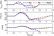
(b) Vehicle steering command, LTR response, and roll response. The dashed blue line is the reference command. The dot-and-dashed red and the solid black lines are the LRG commands with $k_{LRG}\in\left[0,1\right]$ and allowing command contraction, respectively.

Figure 8: Feasibility recovery - LRG with command contraction allowed.

In its standard form, the LRG computation limits the LRG gain to be $k_{LRG}\in\left[0,1\right]$, i.e., the computed command is limited to the interval $\mathbf{v}_{k}\in\left[\mathbf{v}_{k-1},\mathbf{u}_{k}\right]$. With the LRG, there are conditions in which maintaining the last successfully computed command might be problematic. If the solution infeasibility is caused by the differences between the linear model and vehicle nonlinear dynamics, that usually means that the controller allowed the command to be too large, allowing the vehicle state to go too close to the constraints, and maybe breaching them in the near future (fig. 8b). In this case, modifying (26) to allow the command to contract even if the reference command is not contracting produces safer solutions. The computations are modified as follows:

$$\mathcal{S} =\begin{cases}\left[0,\max\left\{\mathbf{v}_{k-1},\mathbf{u}_{k}\right\}\right]&\mathbf{v}_{k-1}>0\>\mathsf{and}\>\mathbf{u}_{k}>0,\\ \left[\min\left\{\mathbf{v}_{k-1},\mathbf{u}_{k}\right\},0\right]&\mathbf{v}_{k-1}<0\>\mathsf{and}\>\mathbf{u}_{k}<0,\\ \left[\mathbf{v}_{k-1},\mathbf{u}_{k}\right]&\mathsf{otherwise},\end{cases}$$ (43)

$$\mathbf{v} =\arg\!\min_{\mathbf{v}}\left\{\left|\mathbf{v}-\mathbf{u}_{k}\right||\left(\mathbf{v},\mathbf{x}\right)\in\mathcal{O}_{\infty}\>\mathsf{and}\>\mathbf{v}\in\mathcal{S}\right\}.$$ (44)

Figure 8b shows that with the last successful command (RG) the vehicle actually breaches momentarily the imposed constraints, $LTR<-100\%$ close to $t=1.9s$, while with the contracted command (RGCC) the LTR is kept within the desired bounds and the command converges to reference value sooner ($@t\approx 1.9s$).

III-F3 $\mathcal{O}_{\infty}$ Set Constraints Temporal Removal

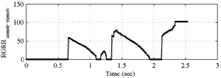
(a) Number of rows removed from the LRG $\mathcal{O}_{\infty}$ set.

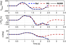
(b) Vehicle steering command, LTR response, and roll response. The dashed blue line is the reference command. The dot-and-dashed red and the solid black lines are the LRG commands blocking and allowing the $\mathcal{O}_{\infty}$ set rows removal, respectively.

Figure 9: Feasibility recovery - $\mathcal{O}_{\infty}$ set rows removal.

This method is based on the premise that the controller might not be able to avoid the constraint violation in the near term, but will be able to bring the system into the desired operation envelope in the future. The method removes as many initial rows from the representation of the $\mathcal{O}_{\infty}$ set as required to make the command computation feasible (alg. 1). In Algorithm 1, $\mathbf{A}_{\mathcal{O}_{\infty}}^{2il+1:2\left(Nl+2\right)}$ is the matrix composed by all rows between the $\left(2il+1\right)th$ line and the last ($2\left(Nl+2\right)th$ row) of the $\mathbf{A}_{\mathcal{O}_{\infty}}$ matrix.

$i=0$

while $\mathbf{v}\>computation\>fails$ do

       $i=i+1$

       $\mathbf{A}^{\prime}_{\mathcal{O}_{\infty}}=\mathbf{A}_{\mathcal{O}_{\infty}}^{2il+1:2\left(Nl+2\right)}$

       $\mathbf{b}^{\prime}_{\mathcal{O}_{\infty}}=\mathbf{b}_{\mathcal{O}_{\infty}}^{2il+1:2\left(Nl+2\right)}$

end while

Algorithm 1 Constraint removal from the $\mathcal{O}_{\infty}$ set.

Figure 9a indicates the number of rows that had to be removed at each computation step to make the command computation feasible. As shown by Figure 9b, this approach (RGRR) is prone to failure, limiting the steering angle only very slightly ($@t\approx 1.35s$) and allowing the car to rollover.

III-F4 $\mathcal{O}_{\infty}$ Set Constraints Relaxation

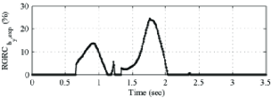
(a) LRG constraint relaxation magnitude.

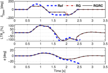
(b) Vehicle steering command, LTR response, and roll response. The dashed blue line is the reference command. The dot-and-dashed red and the solid black lines are the LRG commands without and with constraint relaxation, respectively.

Figure 10: Feasibility recovery - $\mathcal{O}_{\infty}$ constraints relaxation.

The logic behind this approach is that by allowing the controller to find a feasible solution through constraint relaxation, a solution may be found that unfreezes the command computation. This allows the controller to find a solution that may lead to a behavior closer to the intended than a locked command. The method expands and contracts the $\mathcal{O}_{\infty}$ set by modifying the $\mathbf{b}_{\mathcal{O}_{\infty}}$ vector:

$$\mathbf{b}^{\prime}_{\mathcal{O}_{\infty}}=\left(1+\epsilon\right)\mathbf{b}_{\mathcal{O}_{\infty}},$$ (45)

where $\epsilon$ is the expansion factor. This factor is doubled until the command computation is successful and then the bisection method is used to find the minimum $\epsilon$ for which the command computation is feasible.

Figure 10a shows the constraint expansion factor that had to be used at each computation step to make the command computation feasible. Figure 10b shows that this method (RGRC) provides only a small improvement over the last successful command (RG) by allowing the command to converge to the reference value sooner ($@t\approx 2.0s$). It still allows the LTR to breach the imposed constraints ($@t\approx 1.9s$).

We note that various heuristic and sensitivity-based modifications can be proposed where only some of the constraints are relaxed but this entails additional computing effort which is undesirable for this application. Note also that a soft constraint version of the RG has been proposed in [21]; this strategy has not been formally evaluated as it is similar to our $\mathcal{O}_{\infty}$ set constraints relaxation approach.

We also note that for the ECG a similar constraint relaxation method could be implemented, where a relaxation variable is included as part of the Quadratic Programming (QP) and the constraints that are most violated are relaxed first.

III-F5 Selected Feasibility Recovery Method

From the different methods tested with the LRG, the command contraction method was the best performing (sec. IV-C and fig. 19). In the simulations section, except for the results comparing directly the infeasibility recovery methods, the LRG is tested with the command contraction method.

III-G Nonlinear Reference Governor (NRG)

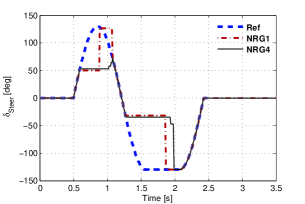
(a) Steering command.

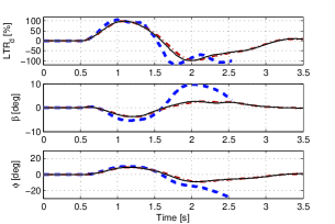
(b) Vehicle lateral response.

Figure 11: Nonlinear Reference Governor command with 1 and 4 nonlinear iterations per step.

The NRG relies on a nonlinear model in prediction to check if a command is safe or, if otherwise, compute a safe command. Instead of the $\mathcal{O}_{\infty}$ set used by the LRGs, the NRG uses a nonlinear model (sec. II-A1) to predict the vehicle response to a constant command for the specified time horizon, usually comparable to the settling time. If the predicted vehicle response stays within the imposed constraints, the command is deemed safe and is passed on. Otherwise, the NRG uses bisections to find a safe command in the range between the last passed (safe) command and the reference command. Each iteration, including the first with the reference command, involves a nonlinear prediction of a modified by bisections command, checks if it respects the constraints, and classifies the command as safe or unsafe. These bisection iterations numerically minimize the reference-command difference, i.e., the difference between the reference command and the used safe command. The number of iterations is a configuration parameter, and governs the balance between the computation time and the solution accuracy. Parametric uncertainties can be taken into account following the approach in [22], but these developments are left to future work.

Figure 11 shows that the NRG with a single iteration (NRG1), i.e., a simple verification of the trajectory constraints with the reference command, produces very similar results when compared with the NRG with three extra bisections (NRG4). The NRG4 initially allows a slightly less constrained command and then has slightly smoother convergence with the reference command ($@t=0.8s\>\&\>1.7s$). This behavior is obtained at the expense of the computational load, taking about 4 times longer to compute a safe command when the reference is unsafe. For the illustrated example (fig. 11), the NRG1 and the NRG4 take an average of $0.16s$ and $0.31s$, respectively, to compute a safe command.

IV Simulation Results

IV-A Simulation Setup

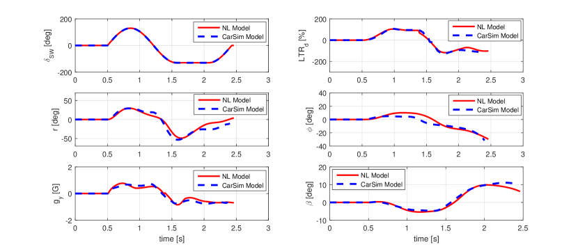
Figure 12: Vehicle dynamics in a Sine with Dwell maneuver. Comparison between the trajectories simulated by a CarSim model and the nonlinear model (sec. II-A).

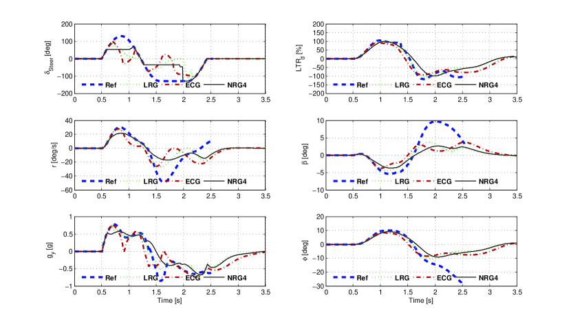
Figure 13: Vehicle dynamics in a Sine with Dwell maneuver. Comparison between the trajectories generated with the intervention of the proposed reference governors.

IV-A1 Simulation Model

The nonlinear simulation model was setup to have a behavior similar to a North American SUV. The model parameters are listed in Table II.

TABLE II: Vehicle simulation parameters.

Parameter	Value
$l_{f}$	$1.160m$
$l_{r}$	$1.750m$
$T$	$1.260m$
$h_{SM}$	$0.780m$
$h_{UC}$	$0.000m$
$m$	$2000kg$
$m_{SM}$	$1700kg$
$m_{UC}$	$300kg$
$I_{xx,SM}$	$1280kg/m^{2}$
$I_{xx,UC}$	$202kg/m^{2}$
$I_{yy,SM}$	$2800kg/m^{2}$
$I_{zz}$	$2800kg/m^{2}$
$I_{xz,SM}$	$0kg/m^{2}$
$k_{\delta_{SM}}$	$17.5$
$K_{S}$	$73991N.m$
$D_{S}$	$5993N.m.s/rad$
$\overline{\Delta k}_{ss}$	$0.0\%$
$\overline{\Delta d}_{ss}$	$0.0\%$

We used a CarSim^® simulation model to check the realism of the nonlinear model presented in section II-A, implemented in MATLAB^®. Figure 12 illustrates the simulation results from both models in terms of their lateral dynamics. The lateral dynamics match very well. All variables except for the roll angle match both in trend and amplitude. The roll angle matches in trend, but shows a larger amplitude in our MATLAB^® model. More importantly, both simulations match very well in terms of the main rollover metric, the LTR. The simulations diverge more in the last moments, when the roll angle is increasing and the car is in the process of rolling over.

IV-A2 Test Maneuvers

National Highway Traffic Safety Administration (NHTSA) defines several test maneuvers: Sine with Dwell, J-Turn, and FishHook [1]. In this work, we chose to test the controllers and demonstrate rollover avoidance for Sine with Dwell maneuvers (fig. 12).

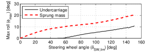
(a) Sprung mass and undercarriage maximum roll angles.

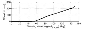
(b) Maximum wheel lift.

Figure 14: Variation of the roll propensity for Sine with Dwell maneuvers. The Sine with Dwell maneuvers vary in terms of steering amplitude, defined by the limit steering angle ($\delta_{SW,lim}$).

Figure 14b illustrates the variation of the vehicle roll (spring mass and undercarriage) and of the maximum wheel lift ($h_{WL,max}=T\sin\left|\phi_{uc,max}\right|$) with respect to the maximum value of the Sine with Dwell reference steering angle, showing $\approx 20deg$ of sprung mass roll and $\approx 240mm$ of wheel lift for $\delta_{SW,lim}=150deg$.

IV-B Trajectories with the Reference Governors (RGs)

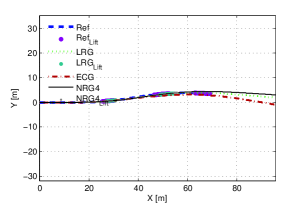
Figure 15: Vehicle trajectory in a Sine with Dwell maneuver.

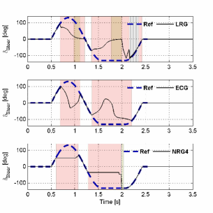
Figure 16: Reference Governors activation, i.e., steering command modification.

Figures 13 and 15 illustrate the effect of the various RGs on the vehicle trajectory. The simulations have been performed on our nonlinear vehicle dynamics model in MATLAB^®. The Linear Reference Governor (LRG) used in this comparison uses the nonlinear difference compensation (sec. III-E1), the Multi-Point Linearization (MPL) (sec. III-E2), and allows command contraction (sec. III-F2). The Extended Command Governor (ECG) uses the MPL (sec. III-E2) and maintains the last successfully computed command sequence (sec. III-F1) when an infeasible command computation is found. The Nonlinear Reference Governor (NRG) performs 4 iterations to find a suitable command, when the reference command is deemed unsafe.

It is clear from Figure 13 that the RGs steering adjustments are different in shape, but not so much in their effect on the LTR, side-slip ($\beta$), roll ($\phi$), and lateral acceleration ($g_{y}$). The amplitude of the turn rate ($r$) is more limited by the NRG than the other RGs. The trajectories with the RGs do not diverge much from the trajectory with the reference steering command, up to the moment when the vehicle starts to rollover with the reference command (fig.  15). The $Ref_{Lift}$, $LRG_{Lift}$, and $NRG4_{Lift}$ shades over the x-y trajectory illustrate where the LTR breaches the imposed constraints.

Figure 16 highlights with background shades when the RGs are active, adjusting the steering command. The darker shades indicate that the controller was unable to avoid breaching the LTR constraints. The LTR plots in Figures 13 and 16 show that in this simulation instance the LRG allowed the LTR to slightly exceed the constraints ($@t\approx 1s\>\&\>1.8s$), but was able to maintain the roll angle well under control.

IV-C Reference Governors Performance Comparison

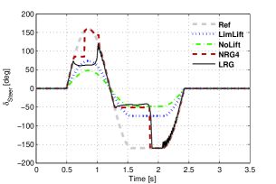
(a) Steering command.

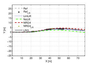
(b) Vehicle trajectory on the X-Y plane.

Figure 17: Reference safe trajectories used for the reference governors performance evaluation. The Ref trajectory is the unmodified sine-with-dwell maneuver with the maximum steering angle defined for a specific test, in this case 160 degrees. The LimLift trajectory is the sine-with-dwell maneuver that produces the maximum allowable wheel lift (5 cm, 2”). The NoLift trajectory is the sine-with-dwell maneuver with the maximum steering angle that produces no wheel lift. The NRG4 trajectory illustrates the safe maneuver, resulting from the Nonlinear Reference Governor intervention, that is considered to interfere the least with the original trajectory (Ref), while avoiding almost completely wheel lift conditions. The LRG trajectory illustrates a maneuver resulting from the application of the Linear Reference Governor.

The results presented next characterize the performance of the controllers in terms of constraint enforcement effectiveness, the adherence to the driver reference (conservatism), the adherence to the desired turning rate (turning response), and the controllers’ computation time. The results were obtained from simulation runs with a range of Sine-with-Dwell maneuvers’ amplitudes between 10 and 160 deg.

Figure 17 illustrates the trajectories that serve as reference in the RGs’ performance evaluation and an example of a trajectory with a controller intervention (LRG). The reference safe trajectories used in (20) and (21) are: the reference trajectory, produced by the original command; the limit lift trajectory (LimLift), with the maximum allowable wheel lift (5 cm, 2”); the no lift trajectory (NoLift), that produces no wheel lift; and the quasi-optimal safe trajectory (NRG4), produced by an NRG with 4 iterations. Each reference safe trajectory has its own merits in the evaluation of the reference governors’ conservatism. The trajectory produced by the reference governors will be the least conservative when compared with the NoLift trajectory. This shows how much the controller reduces the conservatism when compared to a simplistic safe trajectory. The comparison with the NRG4 trajectory produces a middle range conservatism evaluation, allowing us to compare the reference governors’ command with an almost optimal constraint enforcement strategy. The reference governors’ trajectory will be the most conservative when compared with the LimLift trajectory. This shows how much leeway exists between the reference governors’ commands and the commands that produce the limit lift condition.

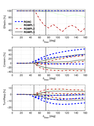
Figure 18: Variation in performance of the LRG with a single linearization point (RGNC - LRG with just the nonlinear difference compensation) and different selections of MPLs (RGMPL#).

The two bottom plots in Figure 18 illustrate the comparison between different LRG options and the NoLift, NRG4, and LimLift reference safe trajectories. On all the figures that illustrate the conservatism and turning response for the same controller configuration, there are three comparison branches, where the NoLift and the LimLift trajectories offer the most advantageous and most disadvantageous comparison trajectories, respectively. That means that the NoLift branch is the bottom branch in the conservatism plots and the top one in the turning response plots (fig. 18). The middle branch, the comparison with a trajectory considered to be NRG4, is the most interesting, as it shows a comparison with one of the least conservative trajectories that produce almost no wheel lift.

Figure 18 shows how the LRG performance improves with Multi-Point Linearization (MPL) and how it changes with the selection of linearization points:

• RGMPL1: 0, 20, 40, and 100 $deg$;

• RGMPL2: 0, 80, 110, and 150 $deg$;

• RGMPL3: 0, 20, 40, 60, 80, 100, 120, 130, 140, and 150 $deg$.

Note that fewer linearization points might lead to less conservatism and a better turning response, however may also result in a worse effectiveness (fig. 18). With a dense selection of linearization points (RGMPL3 case), the LRG is $100\%$ effective for all amplitudes of the reference command.

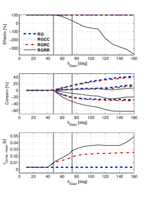
Figure 19: Variation in performance of the MPL LRG (RGMPL3’s linearization points) with the different feasibility recovery methods: last successful command (RG), command contraction (RGCC), constraints’ relaxation (RGRC), and constraint temporal removal (RGRR).

The feasibility recovery methods are compared with the linearization points of the RGMPL3 case (fig. 19). From the various feasibility recovery methods presented in Section III-F, the constraint temporal removal (RGRR), where rows from the $\mathcal{O}_{\infty}$ are removed, is the worst performing. The other three methods, last successful command (RG), command contraction (RGCC), and constraints relaxation (RGRC), are similar in terms of the conservatism metric. The last successful command (RG) method requires the lowest computational overhead. Nevertheless, the command contraction (RGCC) method is preferred, because it provides better effectiveness than the other three methods when the state estimation includes some noise (sec. IV-D).

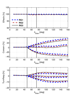
Figure 20: Variation in performance of the MPL LRG allowing contraction for different choices of $LTR_{max}$. $LTR_{max}=99,\>102,\>\&\>105\%$ for RG1, RG2, and RG3, respectively.

Most of the RGs’ tests shown were run with an LTR constraint of $0.99$ or $99\%$. The LTR constraint upper bound can be relaxed, as shown in Figure 20, to reduce the controllers’ conservatism. For $LTR_{max}=99,\>102,\>\&\>105\%$, the effectiveness is only slightly degraded and the conservatism is reduced about $10\%$ from $LTR_{max}=99\%$ to $LTR_{max}=105\%$. Note that the relaxation of the LTR constraint beyond $100\%$ is an ad hoc tuning method, without any guarantees on the effectiveness performance.

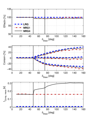
Figure 21: Variation in performance of the LRG, NRG1, and NRG4.

As expected, the NRG for a single iteration (NRG1), i.e., with a check of the actual reference command, runs faster than the NRG setup for four iterations (NRG4) (bottom plot of fig. 21). The unexpected result is that the NRG1 setup is less conservative and has higher effectiveness (top plots of fig. 21). This happens with Sine with Dwell maneuver, because the NRG1 is slightly more conservative during the increment of the reference command, i.e., the moment at which the NRG command diverges from the reference command, but that produces an earlier convergence with the reference command (fig. 11), while the NRG4 takes longer to converge, with a much larger difference between the reference command and the NRG command.

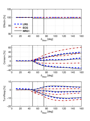
Figure 22: RGs’ performance without estimation errors.

Figure 22 illustrates the performance of the LRG, ECG, and NRG, for the selected configurations. The effectiveness is very similar and over $99\%$ for all the RGs (top plot of fig. 22). That means that the RGs keep the wheels from lifting more than $0.5mm$ ($0.02"$) from the ground, even when the reference steering would lead to rollover. The LRG and the NRG are less conservative and provide better turn response than the ECG (bottom plots of fig. 22). For the most demanding conditions (larger reference command amplitudes), both the LRG and the ECG have a mean computation time of about $0.005s$. In the same conditions, the maximum time for the command computation was lower than $0.01s$ for the LRG and about $0.02s$ for the ECG. The NRG has a larger computation time, which is about $0.16s$ per command update step, when the simulation and control update step is $0.01s$. This means that the NRG setup tested is not able to compute the control solution in real-time in MATLAB^® in the computer used for these tests (64-bit; CPU: Intel^® Core™i7-4600U @ 2.70 GHz; RAM: 8 GB). In C++, the NRG would be about 10 times faster. Also, it may be possible to use slower update rates or shorter prediction horizons with NRGs to reduce the computation times, provided this does not cause performance degradation or increase in constraint violation. We note that explicit reference governor [23] cannot be used for this application as we are lacking a Lyapunov function.

IV-D Performance in the Presence of Estimation Error

In this section, we illustrate the variation of the control performance for 3 controllers: a LRG with command contraction, an ECG, and a NRG with a single iteration (NRG1). The controllers are evaluated through Monte Carlo sampling with a range of estimation error conditions in all states used by the controllers: side-slip, turn rate, roll angle, and roll rate.

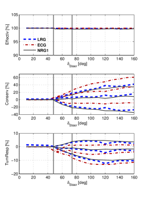
Figure 23: RGs’ performance with estimation errors of $\sigma=10\%$ about the true roll angle.

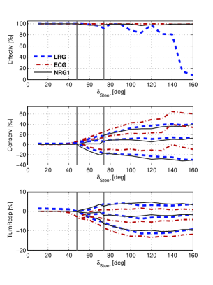
Figure 24: RGs’ performance with estimation errors of $\sigma=20\%$ about the true roll angle.

Figures 23, 24, 25, and 26 illustrate how the errors in the roll angle affect the controllers performance. Figure 23 shows that even with roll estimation errors up to $10\%$, the effectiveness of all the RGs is almost unaffected. Figures 24 and 25 show that the effectiveness of the ECG and the NRG is almost unaffected even for extremely high roll estimation errors. The exception is the LRG controller. Its average effectiveness approaches the limit of 0% for larger reference steering angles, meaning that the wheel could lift an average of $45mm$ ($1.8"$). Figure 25 indicates that this only happens in the presence of very high roll estimation errors and extremely high steering amplitudes ($>140\;deg$).

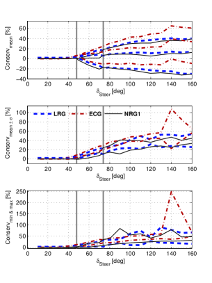
Figure 25: RGs’ effectiveness performance with estimation errors of $\sigma=20\%$ about the true roll angle.

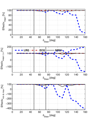
Figure 26: RGs’ conservatism performance with estimation errors of $\sigma=20\%$ about the true roll angle.

Figure 26 shows that the conservatism is also affected by the estimation errors. Nevertheless, even with $20\%$ of estimation error in roll, the RGs conservatism is quite acceptable, and in most test runs it is below $50\%$ for the LRG and NRG and below $60\%$ for the ECG. Most importantly, at lower steering angles, even in the most extreme test runs, the controllers conservatism is kept below 12% for steering angles that would not cause any wheel lift ($\delta_{SW}<48\;deg$) and is kept bellow 35% for steering angles that would take the wheels to reach the limit wheel lift. Among the controllers compared, the ECG controller seems to be the most sensitive to the roll estimation errors in terms of conservatism.

The bottom plots of Figures 23 and 24 show that the controllers turning response is largely unaffected by the estimation errors. Unlike in the conservatism metric, the ECG seems to be the least affected controller.

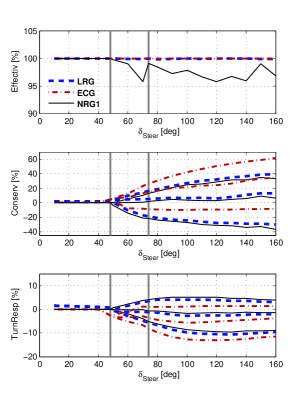
Figure 27: RGs’ performance with estimation errors of $\sigma=20\%$ about the true roll rate.

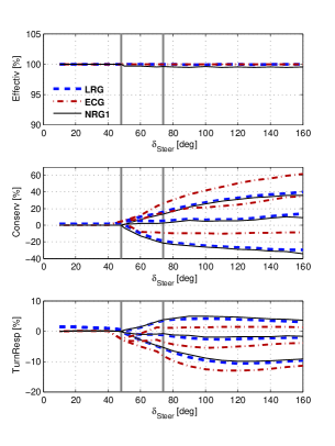
Figure 28: RGs’ performance with estimation errors of $\sigma=20\%$ about the true side-slip angle.

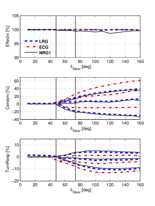
Figure 29: RGs’ performance with estimation errors of $\sigma=20\%$ about the true turn rate.

Figures 27, 28, and 29 show that the controllers’ performance is only slightly affected by roll rate estimation errors and is not visibly affected by the side-slip and turn rate errors, even for the high estimation errors ($\sigma=20\%$).

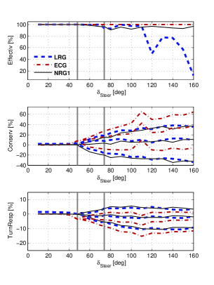
Figure 30: RGs’ performance with estimation errors of $\sigma=20\%$ about the true roll angle and true roll rate.

Figure 30 shows that the effect on the controllers performance from a combination of roll and roll rate estimation errors is very similar to that of just the roll estimation errors. These results show that the controllers are most sensitive to the errors in the roll angle. Nevertheless, the controllers average response is adequate, even with estimation errors with a standard deviation of 20%, which is an extremely poor estimation performance.

V Conclusions and Future Work

V-A Conclusions

We have presented several Reference Governor (RG) designs for vehicle rollover avoidance using active steering commands. We implemented three types of Reference Governors: a Linear Reference Governor (LRG), an Extended Command Governor (ECG), and a Nonlinear Reference Governor (NRG). The goal of the Reference Governors is to enforce Load Transfer Ratio (LTR) constraints. The Reference Governors predict the vehicle trajectory in response to a reference steering command, from the driver, to check if it respects the Load Transfer Ratio (LTR) constraints. The LRG and the ECG use a linear model to check the safety of the steering command. The NRG uses a nonlinear model to achieve the same goal. The controllers were tested with a nonlinear simulation model to check their performance with realistic vehicle dynamics, that are highly nonlinear for large steering angles. The nonlinearity causes the standard versions of the LRG and the ECG to be too conservative. We have presented several methods to compensate for such nonlinearities.

To evaluate the controllers we have defined three performance metrics: effectiveness, conservatism, and turning response. The effectiveness characterizes how well the constraints are enforced by the RG. The conservatism and the turning response characterize if the controller is too intrusive or not, by measuring how well the RG command and respective vehicle trajectory adhere to the driver command and desired trajectory. An additional evaluation metric is the command computation time, that characterizes the controller computational load. The NRG provides the best performance in terms of effectiveness, conservatism, and turning response, but it is slower to compute. The simulation results show that LRG with the nonlinear compensations (nonlinear difference and MPL) provides the best balance between all the metrics. It has a low computational load, while showing very high constraint enforcement effectiveness and generating commands with a conservatism almost as low as the NRG. The simulation results also show that the Reference Governors’ performance is most sensitive to the roll estimation errors, but that even with very high estimation errors ($\sigma=20\%$) the Reference Governors can still enforce the constraints effectively.

VI Further Extensions

Currently we are working to extend the current approach to incorporate differential braking and active suspension commands. It is important to understand the performance limits in rollover avoidance for each individual command. It is also important to understand how the different commands can be combined to provide the most effective and least intrusive rollover avoidance intervention.

Research is also needed to determine the slowest acceptable control update rate, i.e., to characterize how slower update rates degrade the control performance and the driver handling perception.

This research shows that the presented Reference Governors can cope with a great deal of estimation errors. Further research should address the state estimation methodology, given the limited sensing capabilities in standard cars. With such methodology, a better estimation error model should be integrated with the vehicle simulation to verify the Reference Governors performance with a realistic estimation error model. The effects of vehicle and road uncertainties on the estimation and control performance also need to be studied, in order to understand how the system will perform in the range of operating conditions in which the real vehicles will operate.

References

- [1] NHTSA, “49 cfr part 575 - consumer information - new car assessment program - rollover resistance,” Oct 2003.
- [2] A. van Zanten, “Bosch esp systems: 5 years of experience,” in SAE 2000 Automotive Dynamics & Stability Conference, Troy, Michigan, May 2000.
- [3] J. Ackermann and D. Odenthal, “Damping of vehicle roll dynamics by gain scheduled active steering,” in European Control Conference, Karlsruhe, Germany, 1999.
- [4] C. R. Carlson and J. C. Gerdes, “Optimal rollover prevention with steer by wire and differential braking,” in ASME 2003 International Mechanical Engineering Congress and Exposition, Washington, D.C., Nov 15-21 2003, pp. 345–354.
- [5] S. Solmaz, M. Corless, and R. Shorten, “A methodology for the design of robust rollover prevention controllers for automotive vehicles with active steering,” International Journal of Control, vol. 80, no. 11, pp. 1763–1779, Nov 2007.
- [6] P. Koehn and M. Eckrich, “Active Steering - The BMW Approach Towards Modern Steering Technology,” SAE Technical Paper 2004-01-1105, 2004.
- [7] S. Solmaz, M. Corless, and R. Shorten, “A methodology for the design of robust rollover prevention controllers for automotive vehicles - part 1-differential braking,” in 45th IEEE Conference on Decision & Control. San Diego, CA, USA: IEEE, Dec. 13-15 2006, pp. 1739 – 1744.
- [8] ——, “A methodology for the design of robust rollover prevention controllers for automotive vehicles: Part 2-active steering,” in American Control Conference. New York, NY, USA: IEEE, July 9-13 2007, pp. 1606–1611.
- [9] P. Falcone, F. Borrelli, H. E. Tseng, J. Asgari, and D. Hrovat, “Linear time-varying model predictive control and its application to active steering systems: Stability analysis and experimental validation,” International Journal of Robust and Nonlinear Control, vol. 18, no. 8, pp. 862–875, 2008.
- [10] I. V. Kolmanovsky, E. Garone, and S. Di Cairano, “Reference and command governors: A tutorial on their theory and automotive applications,” in American Control Conference (ACC), 2014, Portland, USA, June 2014, pp. 226–241.
- [11] I. V. Kolmanovsky, E. G. Gilbert, and H. Tseng, “Constrained control of vehicle steering,” in Control Applications, (CCA) Intelligent Control, (ISIC), 2009 IEEE, Saint Petersburg, Russia, July 2009, pp. 576–581.
- [12] J. Zhou, “Active safety measures for vehicles involved in light vehicle-to-vehicle impacts,” Ph.D. dissertation, University of Michigan, Ann Arbor, Michigan, USA, 2009.
- [13] A. G. Ulsoy, H. Peng, and M. Çakmakci, Automotive Control Systems. Cambridge University Press, June 2012.
- [14] M. Abe, Vehicle handling dynamics - Theory and applications, 2nd ed. Butterworth-Heinemann, Apr. 22 2015.
- [15] R. Bencatel, I. V. Kolmanovsky, and A. Girard, “Arc-lab technical report 2015-008 - car undercarriage dynamics - wheel lift condition,” University of Michigan - Aerospace Robotics and Control Laboratory, Tech. Rep., 2015.
- [16] D. Karnopp, Vehicle Dynamics, Stability, and Control, ser. Mechanical Engineering. CRC Press, Jan. 22 2013.
- [17] S. Hong, G. Erdogan, J. K. Hedrick, and F. Borrelli, “Tyre–road friction coefficient estimation based on tyre sensors and lateral tyre deflection: modelling, simulations and experiments,” Vehicle system dynamics, vol. 51, no. 5, pp. 627–647, Sep. 24 2013.
- [18] J. L. Stein and J. K. Hedrick, “Influence of fifth wheel location on truck ride quality,” Transportation Research Record, no. 774, pp. 31–39, 1980.
- [19] E. G. Gilbert, I. Kolmanovsky, and K. T. Tan, “Discrete-time reference governors and the nonlinear control of systems with state and control constraints,” International Journal of Robust and Nonlinear Control, vol. 5, pp. 487–504, 1995.
- [20] E. G. Gilbert and C.-J. Ong, “Constrained linear systems with hard constraints and disturbances: An extended command governor with large domain of attraction,” Automatica, vol. 47, no. 2, pp. 334–340, 2011.
- [21] U. Kalabić, Y. Chitalia, J. Buckland, and I. Kolmanovsky, “Prioritization schemes for reference and command governors,” in European Control Conference. Zurich, Swiss: IEEE, July 17-19 2013, pp. 2734 – 2739.
- [22] J. Sun and I. V. Kolmanovsky, “Load governor for fuel cell oxygen starvation protection: a robust nonlinear reference governor approach,” IEEE Transactions on Control Systems Technology, vol. 13, no. 6, pp. 911–920, Nov. 2005.
- [23] E. Garone, S. Di Cairano, and I. V. Kolmanovsky, “Reference and Command Governors for Systems with Constraints: A Survey of Their Theory and Applications,” Automatica, to appear.