Experimental quantum compressed sensing for a seven-qubit system

Abstract

Well-controlled quantum devices with their increasing system size face a new roadblock hindering further development of quantum technologies: The effort of quantum tomography—the characterization of processes and states within a quantum device—scales unfavorably to the point that state-of-the-art systems can no longer be treated. Quantum compressed sensing mitigates this problem by reconstructing the state from an incomplete set of observables. In this work, we present an experimental implementation of compressed tomography of a seven qubit system—the largest-scale realization to date—and we introduce new numerical methods in order to scale the reconstruction to this dimension. Originally, compressed sensing has been advocated for density matrices with few non-zero eigenvalues. Here, we argue that the low-rank estimates provided by compressed sensing can be appropriate even in the general case. The reason is that statistical noise often allows only for the leading eigenvectors to be reliably reconstructed: We find that the remaining eigenvectors behave in a way consistent with a random matrix model that carries no information about the true state. We report a reconstruction of quantum states from a topological color code of seven qubits, prepared in a trapped ion architecture, based on tomographically incomplete data involving $127$ Pauli basis measurement settings only, repeated $100$ times each.

Recent years have seen rapid progress in the development of quantum technologies, with precisely controlled quantum systems reaching ever larger system sizes. Specifically, for systems of trapped ions, precisely controlled arrays of tens and more individual ions have been engineered and manipulated in their quantum state,Nigg et al. (2014); Lanyon et al. (2011); Kaufmann et al. (2012); Blatt and Roos (2012) while architectures such as superconducting qubits Barends et al. (2014); Ofek et al. (2016) and neutral atoms,Maller et al. (2015); Nogrette et al. (2014) among many others, are also developing rapidly. These technological and scientific developments have enabled implementations of small-scale quantum simulators,Lanyon et al. (2011); Kaufmann et al. (2012); Blatt and Roos (2012) small measurement-based quantum computations,Lanyon et al. (2013), proof-of-principle gate-based quantum computations,Vandersypen et al. (2001); Fedorov et al. (2012); Nigg et al. (2014); Gulde et al. (2003) and quantum error correction, e.g. based on topological color codes.Nigg et al. (2014)

As a result of this fast development, a new roadblock is an increasing concern: The fact that the Hilbert space dimension scales exponentially means that traditional methods for the experimental characterization of the processes and states that have been implemented becomes infeasible even for intermediate system sizes. This is problematic, since such systems are relevant as building blocks for emerging quantum technologies. To mitigate this problem, it has been suggested to use various structural properties of natural quantum systems—e.g. high purity, symmetries, sparsity in a known basis, or entanglement area laws—in order to reduce the effort of characterization.Gross et al. (2010); Cramer et al. (2010); Flammia et al. (2012); Flammia and Liu (2011); Shabani et al. (2011); Hübener et al. (2013); Steffens et al. (2015)

In this work, we demonstrate that this approach is reaching maturity by implementing an experimental reconstruction of the state of a 7-qubit system from an informationally incomplete set of measurements. To achieve this, we are relying on the technique of compressed sensing. This theory has emerged over the past decade in the field of classical data analysis.Candes and Wakin (2008); Foucart and Rauhut (2013) It is now routinely used to estimate vectors or matrices from incomplete information, with manifold applications in such diverse fields as image processing, seismology, wireless communication, and many more.Foucart and Rauhut (2013); Eldar (2012) Compressed sensing for low-rank matrices has been adapted as a tool for quantum system characterization (also referred to as quantum tomography) in a series of works.Gross et al. (2010); Flammia et al. (2012); Kueng et al. (2015) A particularly appealing feature of compressed quantum tomography (the combination of compressed sensing and quantum tomography) is the fact that there is no need to make any a priori assumptions about the true quantum state.Carpentier et al. (2015); Flammia et al. (2012)

Quantum compressed sensing is most effective on density matrices with quickly decaying eigenvalues. Such a matrix can be well-approximated by one having a rank $r$ that is much smaller than the dimension $d$ of the Hilbert space. A rank-$r$ matrix depends on only $O(rd)$ parameters, significantly fewer than the $d^{2}$ parameters required in general. In quantum information experiments, the goal is often to prepare a pure state, described by a rank-1 density operator. Noise effects will typically require one to include more than just one eigenvalue to obtain a good approximation of the true density matrix. However, in highly controlled experiments, the number of additional eigenvalues required to obtain an accurate state estimate is expected to be small. In this context, the theory of compressed sensing showed for the first time that the reduced number of parameters is reflected in a reduced effort in both measurements and computation required for tomographic reconstruction. Indeed, it has been rigorously shown that an (approximate) rank-$r$ density matrix can be recovered from $O(rd\log^{2}d)$ experimentally measured parameters.Gross et al. (2010) This performance – close to the absolute lower bound of $O(rd)$ – can even be achieved when the eigenbasis is completely unknown.Gross et al. (2010) A variety of computationally efficient estimators have been proposed to achieve recovery in practice, and we will revisit this topic in more detail below when we describe the numerical implementation we have used for this experiment.

While important steps towards quantum compressed sensing protocols have been implemented before,Rodionov et al. (2014); Schwemmer et al. (2014); Shabani et al. (2011) we report here the first implementation of compressed state reconstruction in an intermediate-sized quantum system. For the purposes of this work, we refer to a quantum system as being intermediate-sized if it has $5$–$10$ physical qubits. This is the range where quantum error correction of one- and two-qubit logical gates becomes possible and full state reconstruction methods are most useful. We do so on the basis of a platform of seven trapped ions, which are prepared in a state of a topological color code.Bombin and Martin-Delgado (2006)

A secondary objective of this work is to argue that compressed tomography, while originally developed for density matrices with a small number of dominating eigenvalues, can also be appropriate in situations where the unknown true density matrix is not, in fact, of low rank. This counterintuitive conclusion follows from the finding that in realistic regimes, the statistical signal-to-noise ratio is such that only the leading eigenvectors of the density matrix can be reliably reconstructed. Indeed, we find that the tail of least-significant eigenvectors behaves in ways consistent with a random matrix model, which means that reporting more than the first few eigenvectors reveals no information about the true state and thus amounts to overfitting. To make this insight more concrete, we formulate a task that is very much reminiscent of support identification in compressed sensing, referring to the problem of deciding which estimated eigenspaces should be included in an estimate (see, e.g., ref. Waters et al. (2011)), which we may call quantum support identification. We give heuristics for identifying the relevant support, based on comparing the behavior of the estimate with a random matrix model. Our findings here are consistent with a recent approach that recommends spectral thresholding for statistical reasons;Guta et al. (2012) and another work that shows that statistical noise in state reconstruction protocols can manifest itself by giving rise to random-matrix like behavior.Knips et al. (2015)

We also observe that the estimators introduced in the context of compressed sensing reconstruct the leading eigenvectors more faithfully than more traditional approaches, at the price of being less faithful on the spectral tail. This suggests that one should employ the former if one is more interested in learning coherent errors (i.e. the way in which the first eigenvector deviates from its target), while the latter are better-suited to analyze incoherent noise processes that drive up the rank. It should be noted that these observations are qualitative rather than mathematically precise at this point.

The rest of this work is organized as follows: We first discuss the physical system at hand and state how the raw data is obtained. We then introduce the estimators used to recover the density operator. Subsequently, we turn to the discussion of quantum identification and to what is called model selection in the literature. We here also discuss the main results of this work and elaborate on the outcomes of the actual reconstruction from experimental data. We conclude by presenting further perspective arising from our approach.

Physical system and raw data

We begin by explaining the physical architecture of trapped ions that serves as the platform for this endeavor. In the considered ion-trap quantum computer, ⁴⁰Ca⁺ ions are stored in a linear Paul trap. Each physical qubit is encoded in $S_{1/2}(m=-1/2)=\lvert 1\rangle$ and the metastable, excited state corresponding to $D_{5/2}(m=-1/2)=\lvert 0\rangle$. Manipulation of the qubit is performed by laser pulses resonant (or close to resonant) to the atomic transitions of ⁴⁰Ca⁺. The universal set of quantum gates is implemented using three types of operations: collective operations of the form $\exp\bigl{(}-i({\theta}/{2})S_{\phi}\bigr{)}$ with

$$S_{\phi}=\sum_{l=1}^{L}\bigl{(}\cos(\phi)X_{l}+\sin(\phi)Y_{l}\bigr{)}\,,$$ (1)

and entangling operations of the form $\exp\bigl{(}-i({\theta}/{4})S_{\phi}^{2}\bigr{)}$, reflecting the entangling Mølmer-Sørenson interaction.Sørensen and Mølmer (1999) Here $X_{l},Y_{l},Z_{l}$ are the Pauli operators of qubit $l$, $\theta=\Omega t$ is determined by the Rabi frequency $\Omega$ and laser pulse duration $t>0$, and $\phi$ is determined by the relative phase between qubit and laser. The third type of operations are generated by single qubit phase rotations induced by localized AC-Stark shifts. More details of this experimental setup are covered in ref. 32.

Within this experimental setting involving $L=7$ qubits, quantum states have been prepared to the best of the experimental knowledge which, however, is limited by statistical noise and systematic errors. The quantum states are described mathematically by density operators $\rho\in\mathbbm{H}_{d}(\mathbbm{C})$ (Hermitian $d\times d$ matrices) for $d=2^{L}$ that satisfy $\mathrm{tr}(\rho)=1$ and $\rho\geq 0$. In all of the experiments, the aim was to prepare a pure state vector which is contained in the code space, which is a two-dimensional subspace of the Hilbert space of seven qubits spanned by $|\bar{0}\rangle$ and $|\bar{1}\rangle$. Here, the state vectors $|\bar{0}\rangle$ and $|\bar{1}\rangle$ span the code space and are joint $+1$ eigenstates of the set of stabilizer operators that define the code. The stabilizer operators are given explicitly in ref. 1. The particular basis for the code space is chosen by picking $|\bar{0}\rangle$ and $|\bar{1}\rangle$ to be the eigenvectors of $Z_{1}\otimes\dots\otimes Z_{L}$ with eigenvalues $+1$ and $-1$ respectively. The states that the ideal experiment would prepare will be referred to as anticipated states in what follows. Both $|\bar{0}\rangle$ and $|\bar{1}\rangle$ are code words of a Calderbank-Shor-Steane code Calderbank and Shor (1996); Steane (1996) originating from the theory of quantum error correction designed to protect fragile quantum information against unwanted local noise. At the same time, they can be seen as the smallest fully functional instances of a topological color code,Bombin and Martin-Delgado (2006) which are topological quantum error-correcting codes defined on physical systems supported on two-dimensional lattices.

For each state, a set of $n=127$ Pauli basis measurement settings is chosen. (An informationally complete set would contain $3^{L}=2187$ settings). Each measurement setting $j$ is characterized by a choice of a local Pauli matrix

$$W_{l}^{(j)}\in\{X_{l},Y_{l},Z_{l}\},\qquad l=1,\dots,L.$$ (2)

for each of the $L$ qubits. The $l$th qubit is measured in the eigenbasis of $W_{l}^{(j)}$. There are two possible outcomes for each qubit, and therefore a total of $2^{L}$ possible outcomes per experiment. Each specific outcome $k$ is associated with a projection operator

$$P^{(j)}_{k}=|v_{k}^{(j)}\rangle\langle v_{k}^{(j)}|,\qquad k=1,\dots 2^{L},$$ (3)

where $|v_{k}^{(j)}\rangle$ is a tensor product of eigenvectors of the $W^{(j)}_{l}$.

For each measurement setting, the measurement is repeated $m=100$ times and the statistics of measurement outcomes is recorded. From the relative frequencies of outcomes $k$, the probability $\mathrm{tr}(\rho P^{(j)}_{k})$ is estimated. Because of the relatively small number of repetitions of the measurements per setting, given $2^{L}$ potential outcomes, many of the possible outcomes will not appear even once.

Let us denote the measurement settings that have been chosen as $V\subset W$, where $W$ is the set of all possible measurement settings. We define the sampling operator $\mathcal{A}:\mathbbm{H}_{d}(\mathbbm{C})\rightarrow\mathbbm{R}^{nd}$ as

$$\mathcal{A}(\rho)=\bigl{(}\mathrm{tr}(\rho P^{(1)}_{1}),\mathrm{tr}(\rho P^{(1)}_{2}),\dots,\mathrm{tr}(\rho P^{(n)}_{d})\bigr{)},$$ (4)

with $n=|V|$ the number of chosen settings. That is, the sampling operator is the linear map that simply returns the list of expectation values of the observables $P^{(j)}_{k}$ measured in the state $\rho$. The data taken are of the type

$$\mathbf{y}=\mathcal{A}(\rho)+\mathbf{z}(\rho),$$ (5)

where the zero-mean random vector $\mathbf{z}(\rho)$ captures the statistical noise. The outcomes for any given basis follow a multinomial distribution, from which one obtains the expression

$$\frac{1}{m}\mathrm{tr}(\rho P^{(j)}_{k})\bigl{(}1-\mathrm{tr}(\rho P^{(j)}_{k})\bigr{)},$$ (6)

for the second moment of each given component of $\mathbf{y}$.

For completeness, we note that the Pauli basis measurements considered here differ from the Pauli correlation measuemrents that were the basis of some previous works on compressed sensing.Gross et al. (2010) Pauli correlation measurements are of the form $\mathrm{tr}\bigl{(}\rho(W_{1}^{(j)}\otimes\dots\otimes W_{L}^{(j)})\bigr{)}$, where again the $W_{l}^{(j)}$ are Pauli matrices acting on the $l$th qubit. These correlators associate one expectation value with each choice of local Pauli matrices and appear e.g. as syndrome measurements in quantum error correction. As detailed above, the basis measurements yield $2^{L}$ parameters per choice of local Pauli matrices. This is the number of ways of picking one of the two eigenvectors of each Pauli matrix. Basis measurements, which thus give much more detailed information per setting, appear naturally in the ion trap architecture used for this work. One can recover Pauli correlations from basis measurements via the relationship

$$\mathrm{tr}\bigl{(}\rho(W_{1}^{(j)}\otimes\dots\otimes W_{L}^{(j)})\bigr{)}=\sum_{k=1}^{d}(-1)^{\chi(k)}\mathrm{tr}(\rho P_{k}^{(j)}),$$ (7)

where $\chi(k)$ denotes the parity of the binary representation of the integer $k$.

Estimators and state reconstruction

In statistics, an estimator is a rule for mapping observed data (here, outcomes ${\mathbf{y}}$) to an estimate for an unknown quantity (here, a density matrix $\rho$). At the heart of the discussion here is an estimator that is particularly common in the compressed sensing literature. This is the so-called matrix Lasso Flammia et al. (2012) defined as

$$\min_{X}\,\|\mathbf{y}-\mathcal{A}(X)\|_{2}^{2}+\mu\|X\|_{*},$$ (8)

where $\mu\geq 0$ is a regularization parameter and $\|.\|_{*}$ is the nuclear or matrix trace norm. (The trace norm can be shown to be the tightest convex relaxation of “rank”. Thus, the regularization term both encourages low-rank solutions and, due to convexity, can be minimized efficiently Foucart and Rauhut (2013)). The estimator does make sense for $\mu=0$ if one adds the additional constraint that the result be positive semi-definite.Kueng et al. (2015) This positivity-constrained least squares estimator will be at the focus of attention in our approach. From its implementation, we expect this estimator to be specifically suited to the regime of intermediate and large quantum systems and comparably little data in which we are interested.

While the estimator from eq. (8) is formally efficient in the sense that it can be solved in polynomial time in the size of the input, additional theoretical efforts are required to arrive at an implementation that performs well in practice in the regime of intermediate and large quantum systems. To achieve this, we here introduce a tailor-made implementation for the $\mu=0$ case. In this approach, we parametrize the quantum state $\rho$ as

$$\rho=Q^{\dagger}Q\,,$$ (9)

for some $r\times d$ complex matrix $Q$, where $r$ controls the rank of $\rho$. We then consider

$$\min_{Q}\,g(Q)=\min_{Q}\,\|\mathbf{y}-\mathcal{A}(Q^{\dagger}Q)\|^{2}_{2},$$ (10)

with $\|.\|_{2}$ is the vector $2$-norm.

Using this parameterization of $\rho$ ensures that it is positive semidefinite by construction. The optimization problem itself is then solved using a gradient method. A gradient flow on the basis of $\rho$ directly would introduce negative eigenvalues in every step. In contrast, we optimize over $Q$, using the fact that we can analytically compute the gradient

$$\nabla_{Q}g(Q)=4Q\mathcal{A}^{\dagger}\bigl{(}\mathcal{A}(Q^{\dagger}Q)-\mathbf{y}\bigr{)},$$ (11)

of the objective function in eq. (10). This way, we dispense with the unnecessary and computationally expensive projection step that would otherwise be needed to enforce positivity.

This simplification significantly improves the computational effort as compared to earlier estimators that made use of an iterative gradient method based on $\rho$. We refer to this gradient method based on a manifestly positive parametrization of states as GRAD. We present details of this algorithm in the appendix.

(a)   Trace norm minimization estimate ($F=0.98$), corresponding to the result of the matrix Lasso in eq. (8) in the limit $\mu\rightarrow\infty$.

(b)   Least squares estimate ($F=0.30$), corresponding to eq. (8) with $\mu=0$.

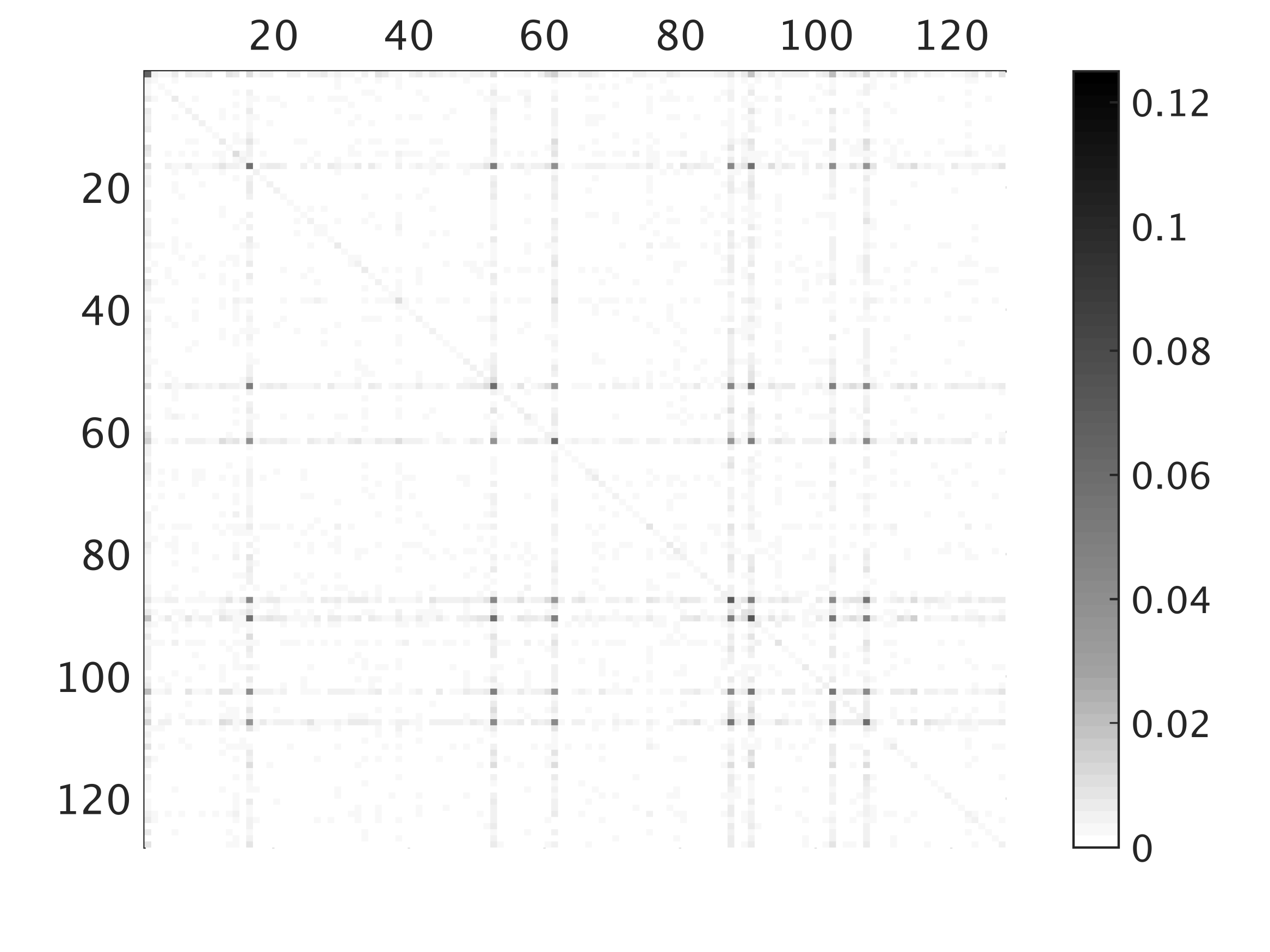
(c)   Rank $21$ leading subspace projection of the least squares estimate ($F=0.32$) obtained by our spectral thresholding method.

Figure 1: Example of quantum state reconstruction for the logical $|\bar{0}\rangle$ state vector. The plots are 2-D plots of the absolute values of the entries of the density matrix in the standard basis with magnitude represented by the grey scale. The axes are labeled by the computational basis vectors. For reasons of clarity, the basis vectors are numbered as $x\in\{1,2,\ldots,d\}$, where $|\chi(x-1)\rangle$ is the state vector in the standard computational basis, $\chi(x-1)$ being the binary representation of $x-1$. So $x=1$ corresponds to $|0,\dots,0,0\rangle$, $x=2$ to $|0,\dots,0,1\rangle$ and so on. The performance of the reconstruction is measured by the fidelity $F=\langle\bar{0}|\hat{\rho}|\bar{0}\rangle$, where $\hat{\rho}$ is the estimated state. While all three estimators produce roughly similar looking estimates, they differ greatly in the fidelity with the anticipated state.

The GRAD method allowed us to analyze data from informationally incomplete measurements on a $7$-qubit trapped ion experiment. In each experiment we have performed, the anticipated states were taken from the code space $\mathrm{span}(|\bar{0}\rangle,|\bar{1}\rangle)$ of the topological color code. In fig. 1, we present a graphical representation of an instance of such a reconstruction. It depicts the anticipated state, the reconstructed one based on the matrix Lasso from eq. (8) with $\mu\to\infty$, the one obtained by positivity-constrained least squares (using $\mu=0$), and an estimator that we call spectral thresholding estimator, to be discussed in more detail below and for reasons that will become clear then, where only the highest eigenvalues have been kept.

From Fig. 1 we see that the estimators give rise to valid and faithful reconstructions of the anticipated state, in that the reconstructed states are close in fidelity to the anticipated states, though some estimators report higher fidelities than others. The computational runtime for the estimators is moreover quite modest, or the order of a few hours, and of a few minutes for the GRAD estimator. This analysis can be seen as a first experimental implementation of quantum state tomography based on a compressed sensing methodology for high-dimensional quantum systems.

If we compare a typical figure of merit for the quality of a state reconstruction—the fidelity to the anticipated state—then we notice the glaring feature that the three reported reconstruction fidelities differ from $F=0.98$ (trace norm minimization estimate) down to $F=0.30$ (least squares estimate) on the same data. We hypothesize that this difference is due to a combination of limited data (applicable to all estimators) and the fact that the Lasso estimator with $\mu\to\infty$ (the trace norm minimization estimate) gives a much higher penalty to mixed states than the other two estimators. Because this trace norm minimization estimator will favor reconstructing nearly pure states, it will not faithfully estimate the tail of the spectrum when data is scarce, but it is expected to be better at diagnosing coherent errors, as it will return the dominant pure state. By contrast, the other estimators sacrifice purity to better match the spectrum, which causes them to have a poor fidelity with the anticipated state. Thus, these estimators might be better for diagnosing incoherent noise, as these methods retain visibility for excessive noise in the system.

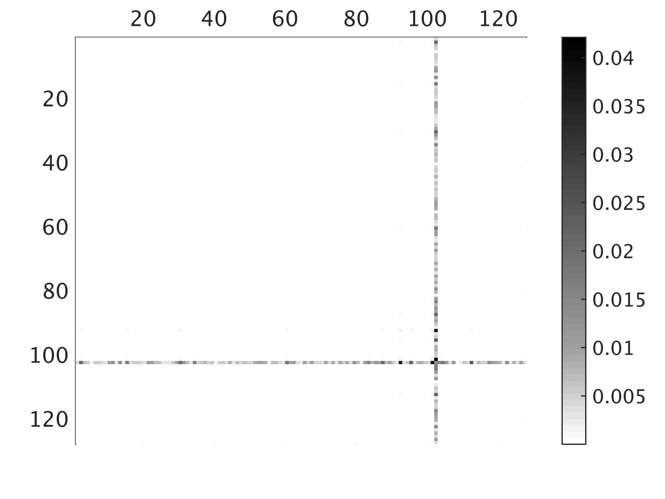
(a)  Trace norm estimate.

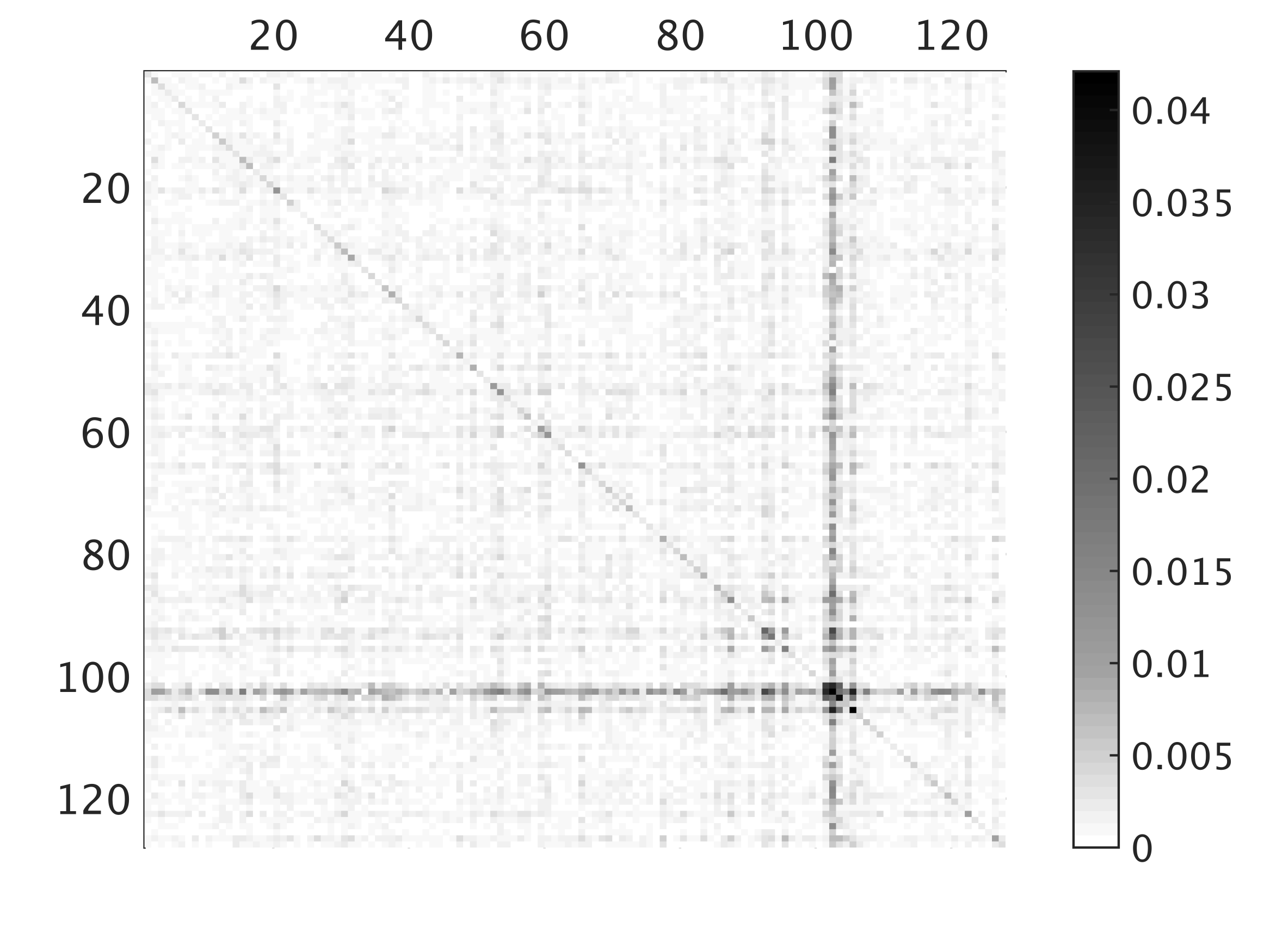
(b)   Least squares estimate.

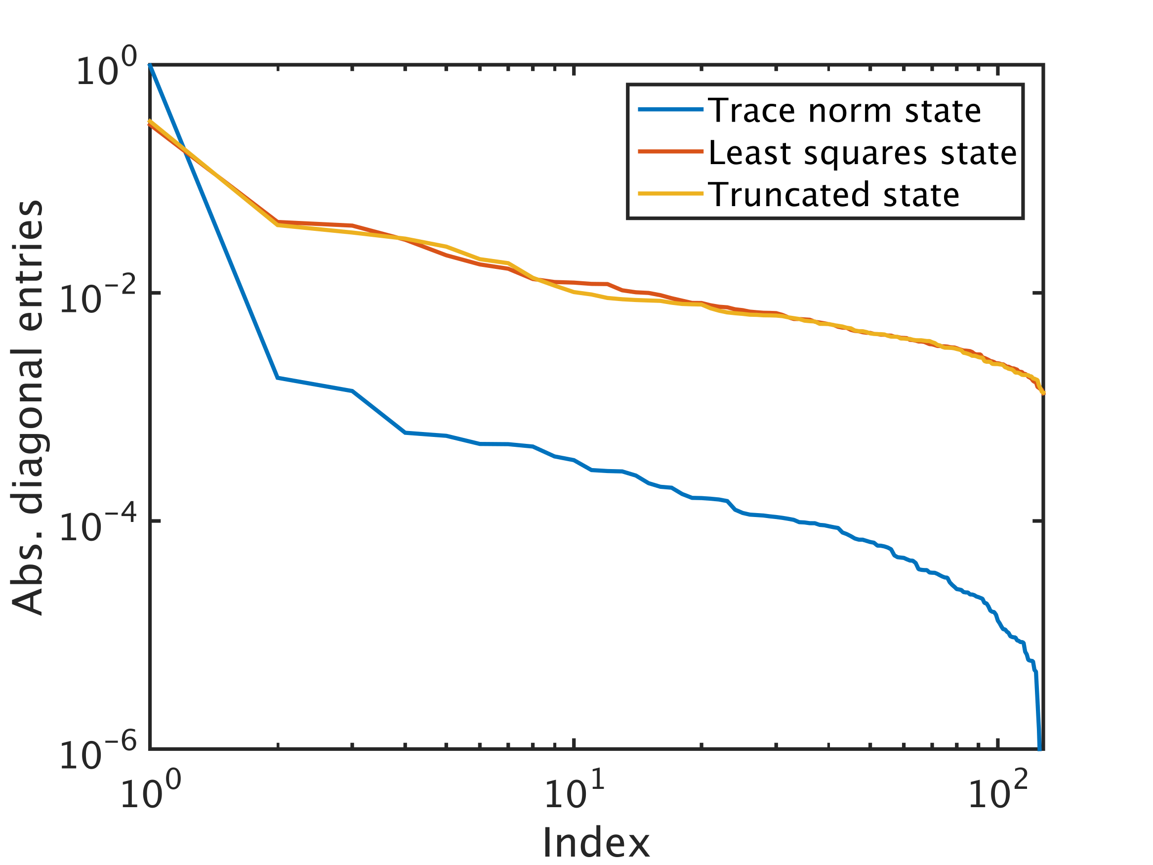
(c)   Diagonal element comparison.

Figure 2: (a,b) 2-D plots of the absolute values of the entries of the difference between the anticipated state and the reconstructed state density matrices in the stabilizer basis of the anticipated state for the logical $|\bar{0}\rangle$ state vector. In this basis, the anticipated state is exactly diagonal with only one nonzero entry in the diagonal. While only the trace norm and least squares estimates are shown, the spectral thresholding estimate is very similar to (b) and is omitted. (c) In the same basis, we plot the diagonal elements of the reconstructed density matrices in order of decreasing magnitude. The log-log plot shows that after a rapid initial decay, most of the diagonal elements follow an exponential decay curve. The trace norm estimator has almost all its support in few diagonal elements and thus is biased heavily towards pure states, while the least squares and spectral thresholding estimators have much heavier tails, despite still exhibiting exponential decay.

We can gather evidence for our hypothesis by looking at the diagonal matrix elements of the reconstructed states in the anticipated basis, meaning the stabilizer basis that includes the anticipated state. In fig. 2(a-b) we see the absolute values of the matrix elements of the reconstructed states using this basis. Here it is much clearer that the trace norm estimate is detecting coherent noise, while the least squares estimate (and the spectral thresholding estimate, not shown) achieve a more mixed reconstruction. In fact, fig. 2(c) shows that in every case the majority of the diagonal elements are decaying exponentially when ordered in decreasing magnitude, but with a much more rapid initial decay for the trace norm estimator. Although this constitutes evidence for our hypothesis, much more work should be done to determine if there is any advantage to using different estimators to highlight different features of the noise.

Quantum support identification

The traditional goal of quantum state tomography is to estimate the true density matrix of the system—i.e. the one that would result in the limit of infinitely many measurements, when all statistical uncertainties have vanished (assuming no drift or other systematic errors). We will now argue that in a high-dimensional setting, with limited data, it may be neither possible nor desirable to obtain a complete estimate of the true state.

It is not necessarily desirable, because it is unclear that a high-dimensional matrix would provide either interpretable or actionable information. Consider a typical use case for tomography, where the difference between the anticipated state and the leading eigenvectors encodes useful information about the dominating error sources. The eigenvectors associated with the first few eigenvalues contain the most useful information about noise effects, and based in these inputs an experimentalist can adjust the apparatus to achieve a higher fidelity in future runs. However, it is unclear which action would possibly follow from knowing, say, the exact form of the 100th eigenvector.

At the same time, the data obtained may also not be sufficient to estimate all the parameters of the full density matrix to a sensible accuracy. Indeed, trying to fit too many degrees of freedom to noisy data results in overfitting, where the estimate depends strongly on statistical fluctuations and only to a small degree on the true state. To combat this, model selection methods give rules for selecting a lower-dimensional model if the amount and variability of the data do not allow for a reconstruction of the full set of unknown parameters.Akaike (1974)

In the context of quantum state estimation, spectral thresholding has been proposed as a model selection method and theoretically analyzed in the regime of informationally complete measurements.Guta et al. (2012) Spectral thresholding here means that a lower-dimensional model is selected by setting all eigenvalues of the estimate to zero that are below a threshold value that depends on the dimension of the Hilbert space and the variance of the individual measurements.Guta et al. (2012)

Here we propose a new heuristic for selecting which eigenvalues of an estimate to keep and which to discard as not meaningful. While it lacks the rigorous guarantees of ref. 29, it is applicable in more general situations. It is based on a transparent criterion: Parameters of an estimated density matrix should not be reported if they behave in ways consistent with a random matrix model—i.e. if they can be explained as resulting from a purely random noise without any signal. This approach is consistent with recent unrelated findings that the spectrum of highly noisy quantum tomographic estimates resembles the spectrum of random matrix models.Knips et al. (2015)

Technically, for a given data set ${\mathbf{y}}^{(1)}$, the spectral decomposition of the positive semi-definite estimate ${\mathbf{y}}^{(1)}\mapsto f({\mathbf{y}}^{(1)})$ can be written as

$$\hat{\rho}^{(1)}:=f({\mathbf{y}}^{(1)})=\sum_{j=1}^{d}\lambda^{(1)}_{j}E^{(1)}_{j},$$ (12)

with decreasingly ordered eigenvalues $\{\lambda_{j}^{(1)}\}$ and corresponding eigenprojections $\{E^{(1)}_{j}\}$. When insufficient data are taken in an experiment, not all eigenprojections can be characterized equally well. Only for some eigenprojections will one have provided sufficient data. They concomitantly will have low uncertainties and thus will be common to different estimates of the same state based on different realizations of the experiment, while the other directions will fluctuate wildly based on the particular data obtained. Generating a different data set ${\mathbf{y}}^{(2)}$ using the bootstrapping techniques detailed below, we arrive at the estimate $f({\mathbf{y}}^{(2)})$ with decomposition

$$\hat{\rho}^{(2)}:=f({\mathbf{y}}^{(2)})=\sum_{j=1}^{d}\lambda^{(2)}_{j}E^{(2)}_{j}.$$ (13)

Our figure of merit is based on the Hilbert-Schmidt scalar product of the eigenprojections

$$M_{j}({\mathbf{y}}^{(1)},{\mathbf{y}}^{(2)})=\text{tr}(E^{(1)}_{j}E^{(2)}_{j}),$$ (14)

where $j=1,\ldots,d$. In the informationally incomplete regime we are in, this quantity will show a strong overlap only between the dominant eigenvectors. For the eigenvectors of the complement, the overlaps resemble the overlap of state vectors chosen randomly from the unitarily invariant Haar measure. In the light of this, the spectral thresholding parameter $k_{\mathrm{max}}$ is taken to be

$$k:=\max\left\{j:\mathbbm{E}\left(M_{j}({\mathbf{y}}^{(1)},{\mathbf{y}}^{(2)})\right)>e_{d}\right\},$$ (15)

in expectation over pairs $({\mathbf{y}}^{(1)},{\mathbf{y}}^{(2)})$, where the threshold $e_{d}$ is chosen as $e_{d}=\mathbbm{E}(x)+\text{var}(x)^{1/2}$ for the random variable defined as $x(U)=|\langle\psi|U|\psi\rangle|^{2}$ as overlaps between Haar random state vectors from $\mathbbm{C}^{d}$. Specifically, a random matrix theory computation (see supplementary material) gives,

$$e_{d}=\frac{1}{d}+\left(\frac{2}{d(d+1)}-\frac{1}{d^{2}}\right)^{1/2}.$$ (16)

Based on such a significance threshold, for the estimate based on the data, we return the spectrally thresholded state $\rho_{k}$ with a normalization $c>0$, where

$$\rho_{k}=c\sum_{j=1}^{k}\lambda^{(1)}_{j}E^{(1)}_{j}\,.$$ (17)

Let us now define the protocol we follow to provide an estimate that has low enough rank to be compatible with few data and yet avoid overfitting. For this, we briefly review the concept of bootstrapping. We consider two types of bootstrapping: parametric and non-parametric bootstrapping. In parametric bootstrapping, from the reconstructed density matrix, one simulates the experimental measurements (sampled according to the appropriate noise statistics) and for each sample data realization one computes a new estimated density matrix. In non-parametric bootstrapping, however, the measured frequencies are assumed as the true probabilities, which in turn are used to simulate (sample) new data sets which are used, as before, to compute an ensemble of estimated density matrices. In both cases, one uses the ensemble of recovered density matrices to gain confidence on the reconstructed state.

The way we proceed is the following: From the experimentally measured frequencies we do either parametric or non-parametric bootstrapping to generate an ensemble of estimated density matrices. We find their spectral decomposition and order their eigenvalues and eigenvectors in descending order as explained above. Then, for all possible pairs of estimated density matrices, we compute the mean of Eq. (14) for all $j$. Finally, we report as the rank of the reconstructed state the largest $j$ for which the quantity $M_{j}$ has an overlap grater than the threshold computed in Eq. (16). The results are shown in part (d) of Fig. 1 and in the supplementary material.

Conclusion and perspectives

Quantum tomography—the task of reconstructing unknown states from data—is a key primitive in quantum technologies. At its heart, it aims at providing actionable advice upon which the experimenter can make the appropriate modifications to an experimental setup. It goes beyond mere certification of the correctness of an anticipated preparation of a quantum state Flammia and Liu (2011); Flammia et al. (2012); Aolita et al. (2015): By learning in what way the actually prepared state deviates from the anticipated one, one can modify the apparatus appropriately to improve performance in future runs.

The purpose of the present work is two-fold. On the one hand, it presents a successful first compressed sensing tomography implementation on a moderately sized quantum experiment, using estimators and reconstruction techniques that are efficient in the Hilbert space dimension. In this way, it demonstrates the potential of using the machinery of the “big data” paradigm to assess quantum systems close to the limit of what is experimentally feasible. More conceptually, on the other hand, we discuss ideas of quantum support identification, related to the question of what quantum state tomography can actually mean in the regime of informationally incomplete data for intermediately sized quantum systems. We advocate a paradigm that only those low-rank states should be reported that have a statistical basis. It is the hope that in both ways we can inspire further work on the certification and reconstruction of quantum states and processes for increasingly large quantum systems, overcoming the roadblock against further development in quantum technologies.

Supplementary material

Grad estimator

In this supplementary material, we present details of the reconstruction sketched in the main text, beginning with the estimators we use. In our approach, we parametrize the density matrix as

$$\rho=Q^{\dagger}Q,$$ (18)

which makes it manifestly positive semidefinite. We then solve

$$\min_{Q}\,g(Q)=\min_{Q}\,\|\mathbf{y}-\mathcal{A}(Q^{\dagger}Q)\|^{2}_{2},$$ (19)

with $\|.\|_{2}$ being the vector $2$-norm. We do this using a gradient search algorithm, but notably for $Q$ and not for $\rho$ itself. This is the key feature of this approach. This estimator derives from the idea presented in ref. 37. The basic iteration step in a sequence of $\{Q_{i}\}$ is

$$Q_{i+1}=Q_{i}-\alpha_{i}\nabla_{Q}g(Q_{i}).$$ (20)

For the moment $\alpha_{i}>0$ is chosen to be a sufficiently small step size, but this can surely be refined to a conjugate gradient method if absolutely necessary, and can hence be refined to increase convergence speed. In our case, the actual gradient can be computed. Note that $g(Q)$ can be written as

$$g(Q)=\sum_{k}(y_{k}-{\rm Tr}(P_{k}Q^{\dagger}Q))^{2},$$ (21)

and its gradient

$$\nabla_{Q}g(Q) = -2\sum_{k}(y_{k}-{\rm Tr}(P_{k}Q^{\dagger}Q))\nabla_{Q}{\rm Tr}(QP_{k}Q^{\dagger})$$ (22)

$$= 4Q\mathcal{A}^{\dagger}(\mathcal{A}(Q^{\dagger}Q)-\mathbf{y}),$$

as stated in the main text. Here, we have used the standard matrix identity $\nabla_{X}{\rm Tr}(XBX^{\dagger})=XB^{\dagger}+XB$ for the particular case in which $B$ is Hermitian. We then iterate the previous equation until reaching convergence. The state is renormalized at the end, as the trace is not constrained in this way. This is an extremely fast and elegant way to incorporate positivity of $Q^{\dagger}Q$.

It is worth mentioning that this approach significantly improves earlier ideas deriving from Refs. 38; 39, in which a gradient method for the state $\rho$ was combined with a suitable projection. Specifically,

$$\min_{X}\,f(X)=\min_{X}\,\|\mathbf{y}-\mathcal{A}(X)\|^{2}_{2},\quad\text{s.t.}\quad X\geq 0$$ (23)

was solved by moving away from the semidefinite program and solving the optimization problem using a gradient search algorithm. The basic iteration is

$$X_{i+1}=\mathcal{P}(X_{i}-\alpha_{i}\nabla_{X}f(X_{i})),$$ (24)

where here $\nabla_{X}$ is the gradient operator with respect to matrix $X$, and $\mathcal{P}(X)$ is a projector that makes the estimated state positive semidefinite. The gradient is explicitly

$$\nabla_{X}f(X)=2\mathcal{A}^{\dagger}(\mathcal{A}(X)-\mathbf{y}).$$ (25)

While this approach also works, the projection significantly slows down the algorithm, hence the need for our method that directly incorporates positivity.

Random matrices

In this supplementary material, we present results from random matrix theory on expected overlaps of random vectors. Specifically, for an arbitrary vector $|\psi\rangle\in\mathbbm{C}^{d}$, we consider the random variable defined by

$$x(U)=|\langle\psi|U|\psi\rangle|^{2}$$ (26)

and moments thereof with respect to the Haar measure. This quantity is easily identified as the overlap of two random vectors from $\mathbbm{C}^{d}$. We compute first and second moments thereof. They can be computed making use of the powerful Weingarten function formalism Weingarten (1978). We find in terms of a Weingarten function $Wg$,

$$\int_{U(d)}dU|\langle\psi|U|\psi\rangle|^{2}=Wg((1),d)=\frac{1}{d}.$$ (27)

The second moments can be expressed as

$$\int_{U(d)}dU|\langle\psi|U|\psi\rangle|^{4} = 2Wg((1,2),d)+2Wg((2,1),d)$$ (28)

$$= \frac{2}{d^{2}-1}-\frac{2}{d(d^{2}-1)}$$

$$= \frac{2}{d(d+1)}$$

using suitable Weingarten functions. The sum over all permutations on two symbols in the relationship between Haar averages and Weingarten functions, $(1,2)\mapsto(1,2)$ and $(1,2)\mapsto(2,1)$, then simply gives rise to the above two terms. These result in the expression for the variance

$$\mathrm{var}(x)=\frac{2}{d(d+1)}-\frac{1}{d^{2}}.$$ (29)

In the main text, the quantity

$$e_{d} = \mathbbm{E}(x)+\mathrm{var(x)}^{1/2}$$ (30)

$$= \frac{1}{d}+\left(\frac{2}{d(d+1)}-\frac{1}{d^{2}}\right)^{1/2}$$

has been derived from this.

Further estimators

In this section, we review some of the estimators used in this work. The first estimator, referred to as LS-SDP, is a least squares estimator with positivity constraint as a semi-definite program (SDP). It solves

$$\min_{X}\,\|\mathbf{y}-\mathcal{A}(X)\|^{2}_{2},\quad\text{s.t.}\quad X\geq 0.$$ (31)

As with other SDP approaches, $\mathcal{A}(X)$ has to be computed in matrix form, which produces an unfavorable scaling of effort and memory resources in the system size. As before, we can use this for the $L=7$ qubit problem if the number of measurement settings is not too large. That is to say, for $n=127$ it is still usable. The positivity constraint on $X$ helps the estimation process, based on the intuition that the set of feasible density operators lies at the intersection of those operators compatible with the data and the positive cone. In practice, one can perform very good estimation with this algorithm, even with informationally incomplete measurements, if the actual state is not too mixed and hence close to the boundary of state space. There is empirical evidence for this observation, which can also made precise Suess et al. (2016).

The second estimator is the trace norm minimizer referred to as TNM: This is an estimator based on a trace minimization with a positivity constraint as an SDP. Here, we solve the following problem

$$\min_{X}\,\|X\|_{*}=\mathrm{Tr}(X),\quad\text{s.t.}\quad X\geq 0,\,\|\mathbf{y}-\mathcal{A}(X)\|^{2}_{2}\leq\epsilon,$$ (32)

which resembles the Dantzig selector Flammia et al. (2012), with $\epsilon>0$ being the error level. It is an estimator based on the intuition derived from compressed sensing that under the restricted isometry property (RIP) Candes (2008), the positive semidefinite trace norm minimizer compatible with the data is the actual state Gross et al. (2010). This estimator can be cast as an SDP, which again means that $\mathcal{A}(X)$ has to be computed in matrix form, with all memory requirements that come along with it as mentioned above. However, for $L=7$ qubits this is again still feasible if the number of measurement settings is not too large (about less than a thousand on a standard workstation). The obvious shortcoming of this estimator—apart from the fact that it will not work for large systems—is the estimation of $\epsilon>0$, as often discussed (see, e.g., ref. Flammia et al. (2012)). This algorithm is designed to generally produce low-rank estimates.

Simulations on spectral thresholding

In order to test our model selection protocol, we perform numerical simulations in a relatively small system of $L=4$ qubits. We proceed by generating random states of fixed rank: in this example, we choose ranks $1$, $2$, $4$, and $8$. These states, which we refer to as the true states $\rho$, are used to simulate the outcomes of a set of $1$, $10$, $16$, $32$, $56$, and $81$ local random measurements. Each simulated measurement, in turn, is done for different repetitions per observable. We choose, for comparison, $5$, $10$, $16$, and $100$ repetitions per measurement setting. More repetitions means less noise in the observed outcomes. Each numerical experiment is repeated $100$ times and the reconstruction of the density matrix is done via eq. (8) with $\mu=0$. Then, we compute our figure of merit $M_{j}$ as indicated in eq. (14). The results are presented in figs. 3-6. It is clear from the plots that the method described in the main text—when given enough measurements—can, in principle, distinguish the correct rank of the true state (see fig. 7). However, in the informationally incomplete low-data regime that we are interested in, it tends to give a lower rank than the true rank. This is indeed a desirable feature since the amount of collected data is not enough to justify a higher rank fit. Additionally, for benchmarking we compute the expected risk defined by

$$\mathbbm{E}\|\rho-\rho_{k}\|_{2}^{2},$$ (33)

where $\rho$ is the true state and $\rho_{k}$ is the reconstructed and truncated state from spectral thresholding. This is shown in fig. 9.

Since the procedure outlined in this work is related to model selection, for completeness we compare our method to the one proposed in ref. 43. There the authors have developed a particular spectral thresholding algorithm that is applied to a reconstructed density matrix via a plain least squares estimator that does not impose the positivity constraint. Even more, their approach is valid for informationally complete measurements and rigorous proofs are given for its performance. In our test, we have modified the approach in ref. 43 to include the positivity constraint (via the LS-SDP estimator) and have naively applied it to the regime of informationally incomplete measurements. As suggested in ref. 43, we choose the threshold parameter as

$$\gamma(\epsilon)^{2}=\frac{2d}{N}\log{\frac{2d}{\epsilon}}.$$ (34)

In our example, we select $\epsilon=0.05$ and set $N$ to be the total number of prepared quantum states used in the simulation of a particular experiment. For every reconstructed density matrix, computed via eq. (8) with $\mu=0$, we calculate its spectral decomposition and set all eigenvalues smaller than $4\gamma(\epsilon)$ equal to zero as prescribed in ref. 43. After this thresholding procedure, the spectrum is no longer normalized, and we correct this by shifting all eigenvalues by the same quantity (as opposed to dividing by its sum). The average rank, over 100 experiments, obtained by this method is shown in fig. 8. It is clear that the method performs well, as expected, for the informationally complete case. However, when not enough measurements are used in the reconstruction, it seems to (on average) estimate a rank that is greater than what our thresholding method gives (see fig. 7). In terms of risk, as defined in eq. (33), and as shown in fig. 10, we cannot see a very clear trend that distinguishes both methods, except that on average they seem to be similar in risk. Furthermore, we should notice that, for the informationally incomplete regime we are interested in analyzing, to date there is not a rigorously proven method for spectral thresholding available yet.

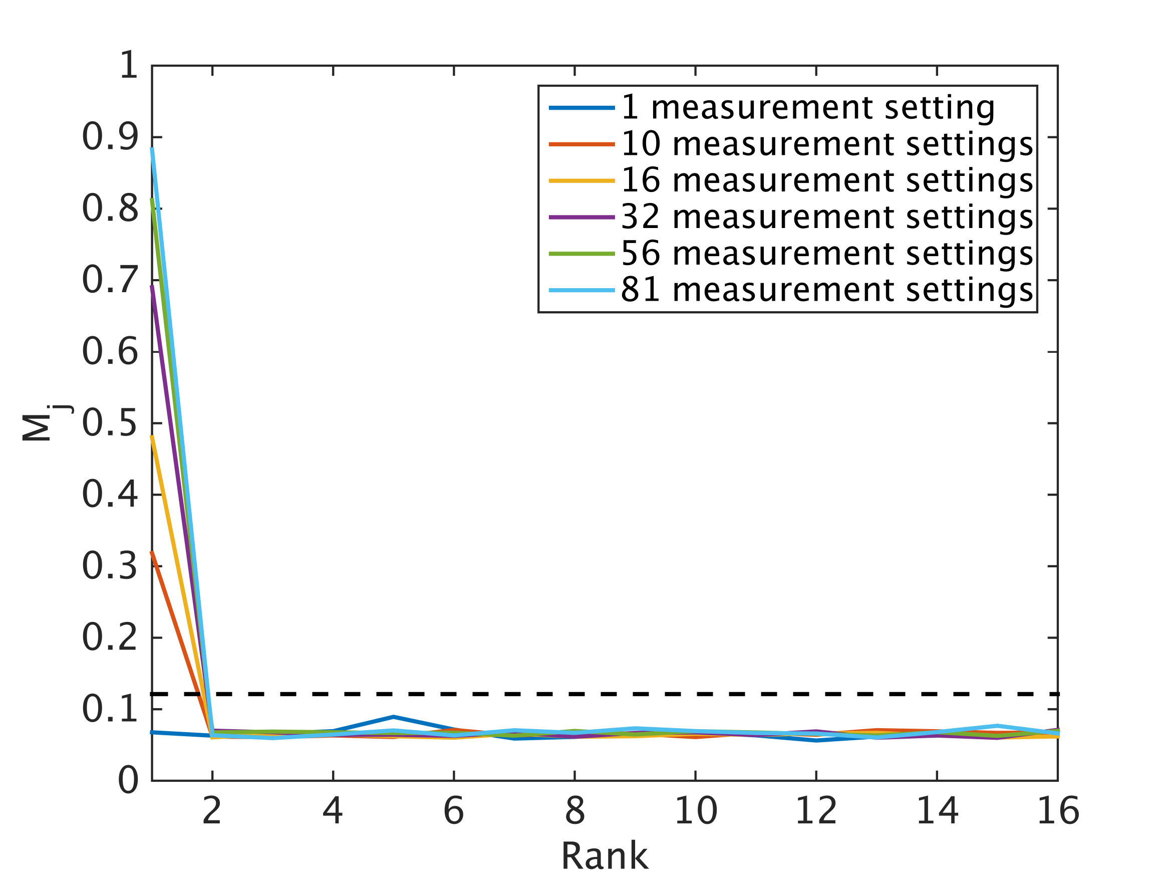
(a)   5 repetitions per measurement setting.

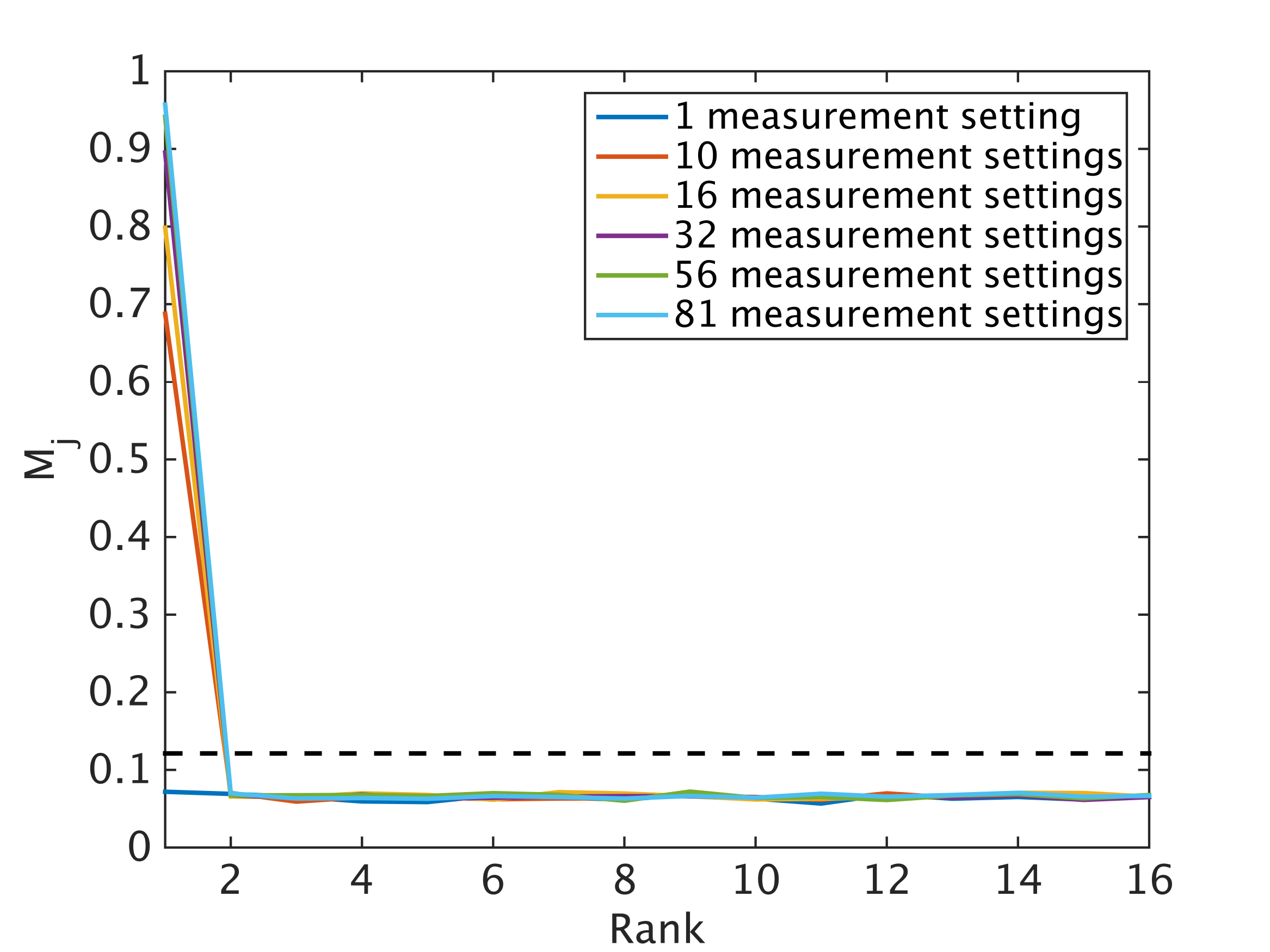
(b)   16 repetitions per measurement setting.

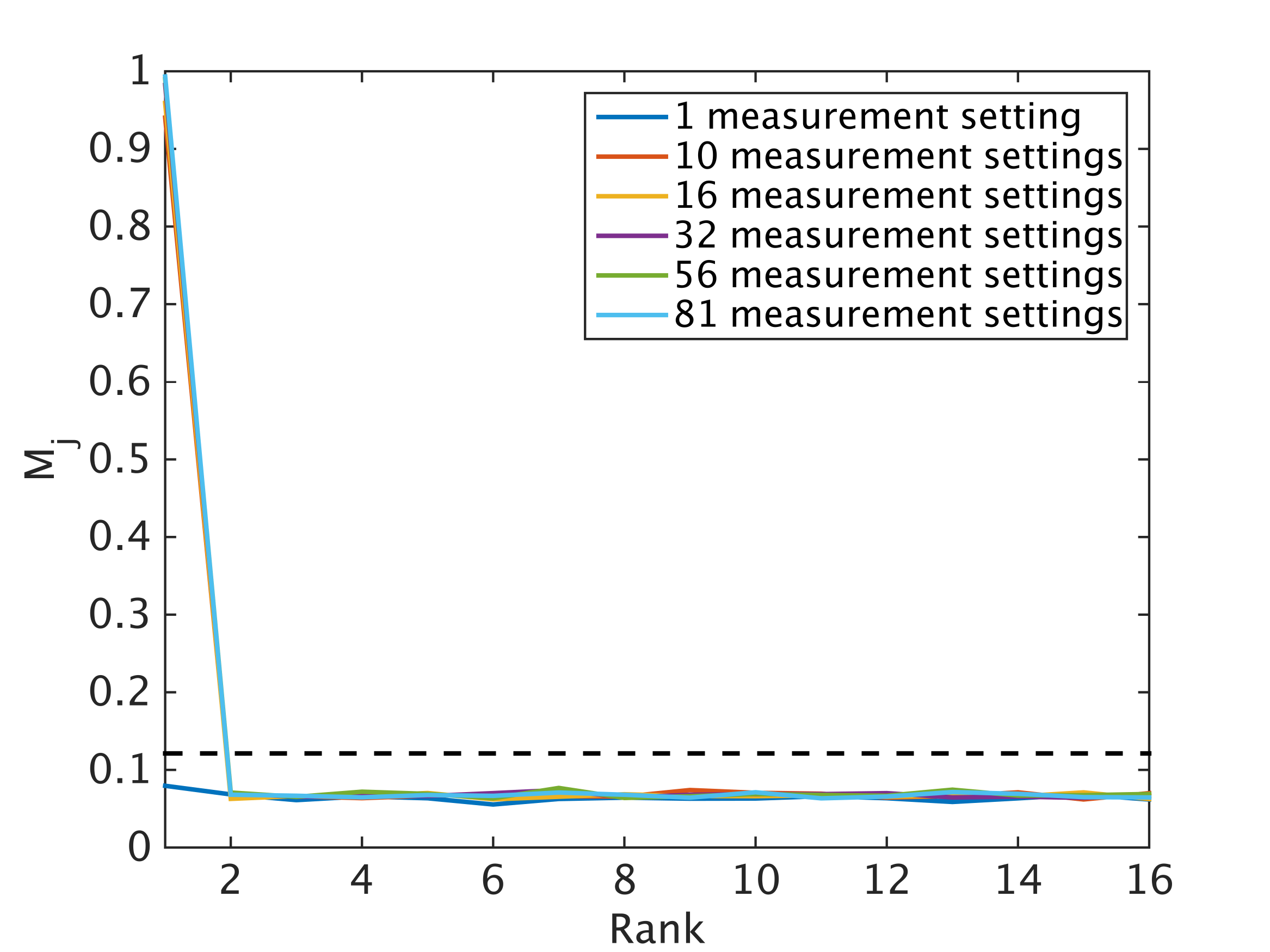
(c)   100 repetitions per measurement setting.

Figure 3: Mean eigenvector overlap as a function of the rank truncation of the recovered density matrix of a true state of rank $1$. The dotted line represents the threshold given in eq. (16).

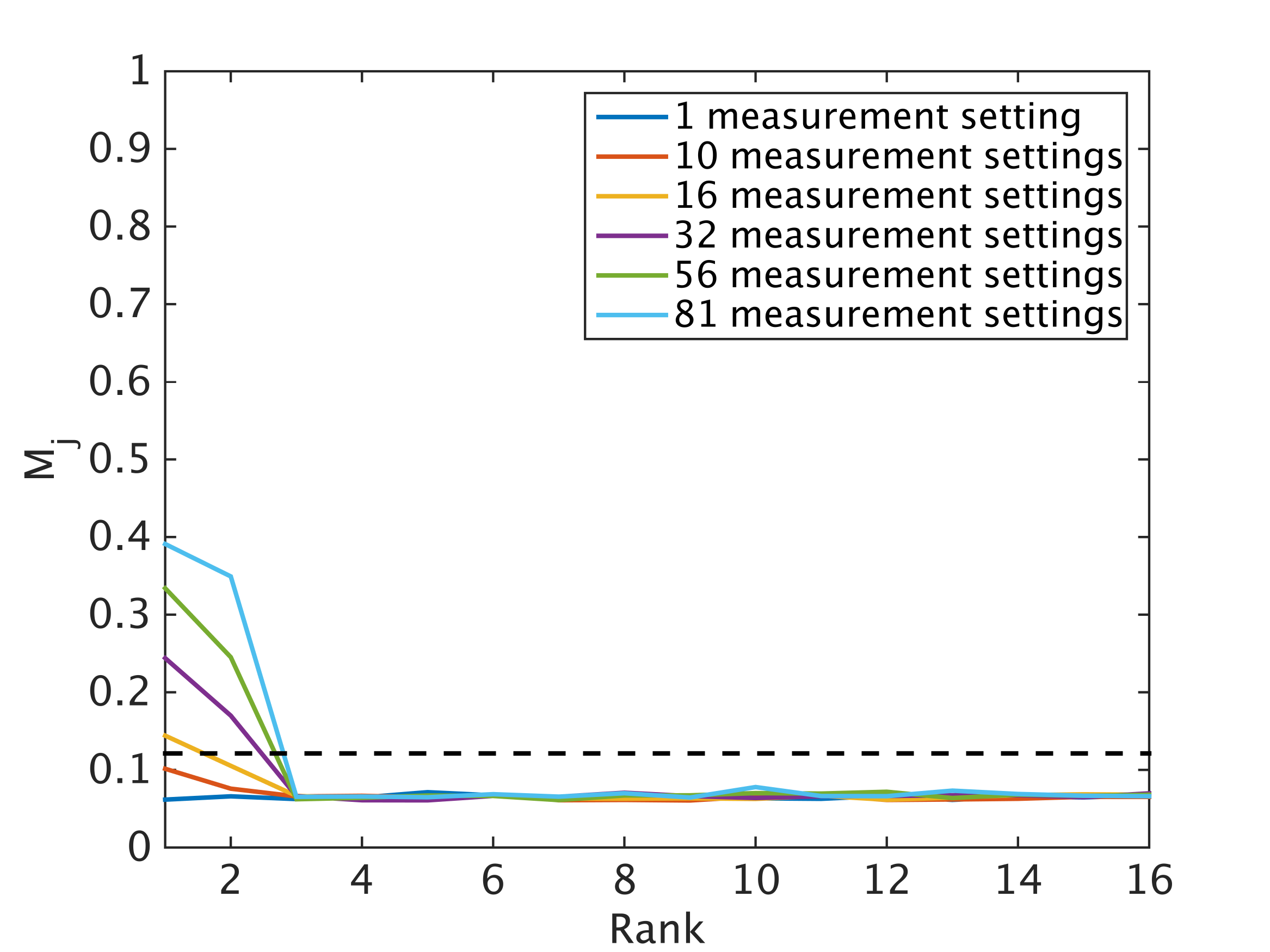
(a)   5 repetitions per measurement setting.

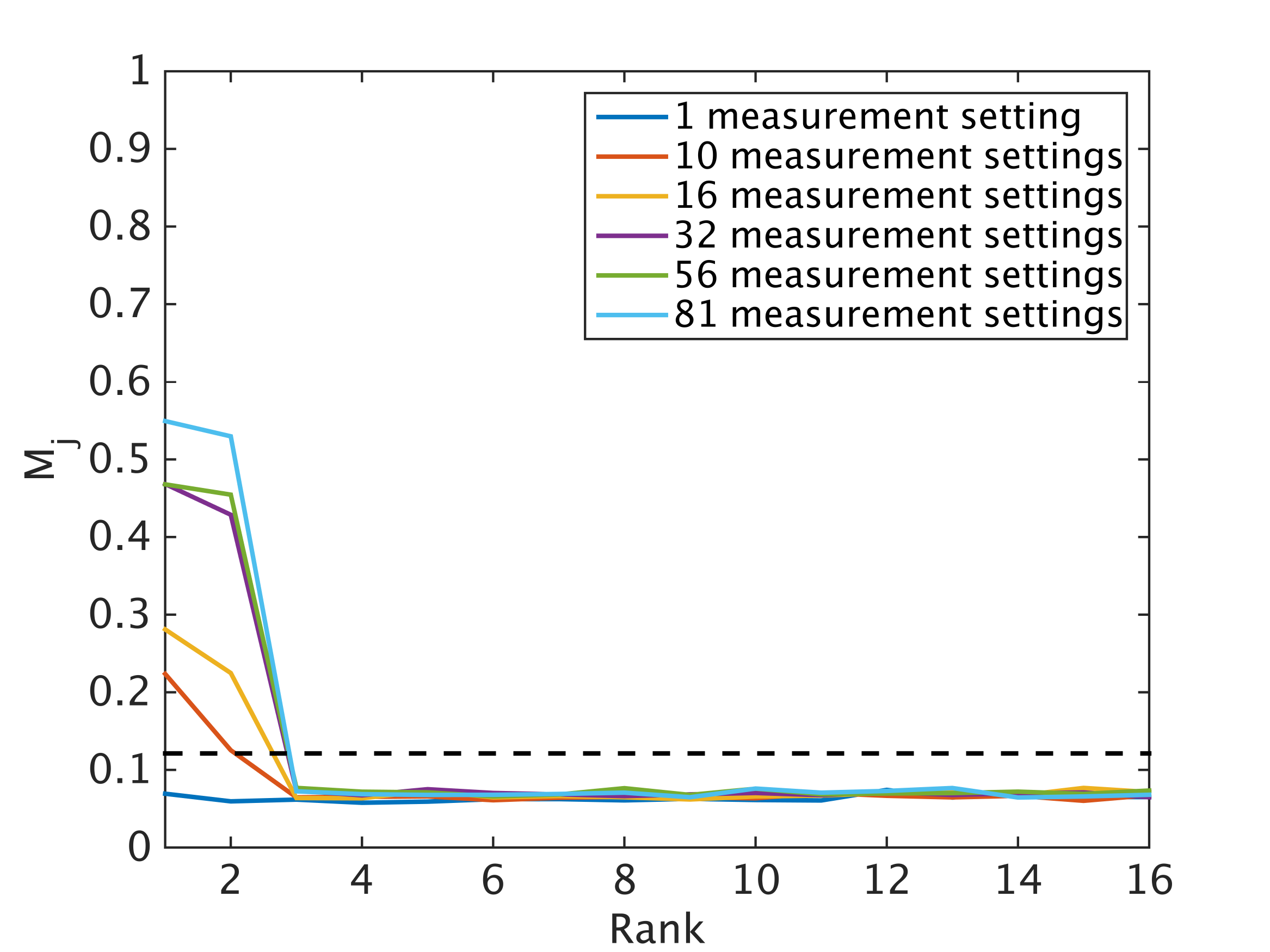
(b)   16 repetitions per measurement setting.

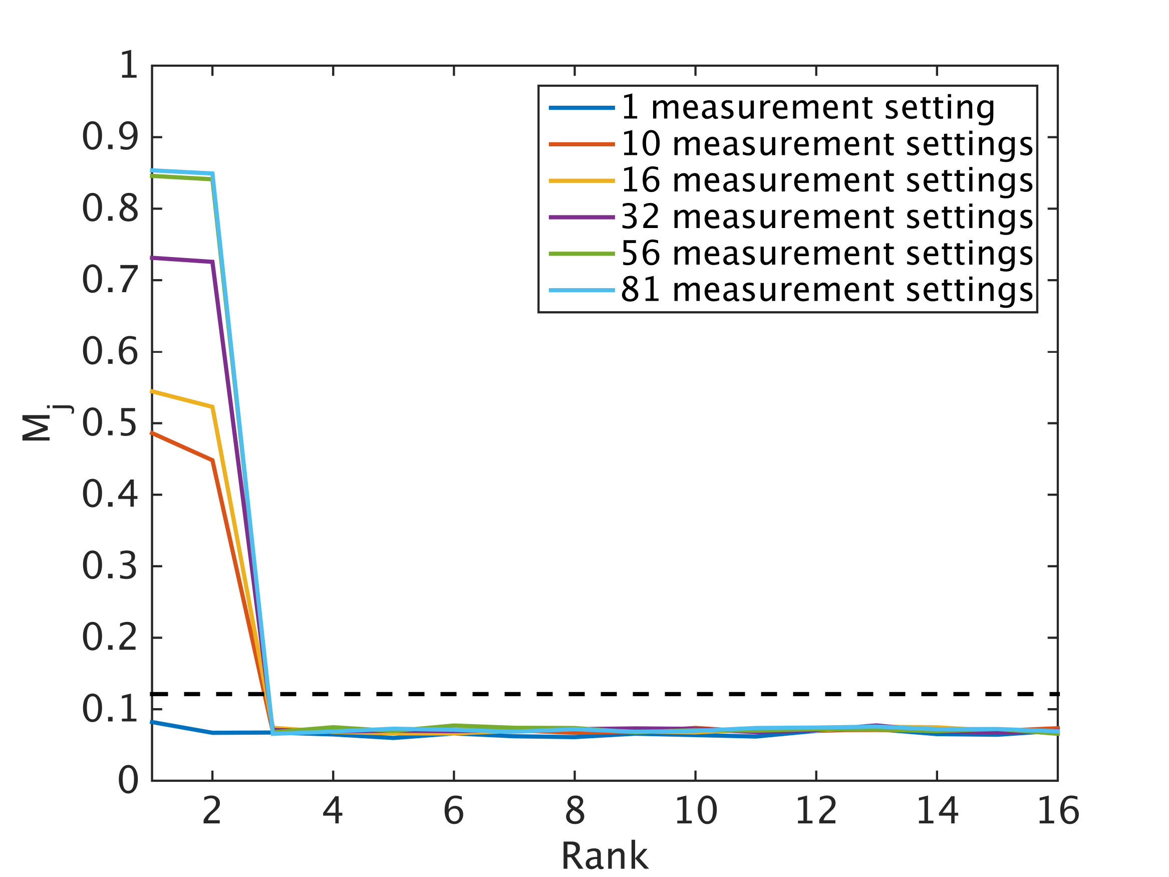
(c)   100 repetitions per measurement setting.

Figure 4: Mean eigenvector overlap as a function of the rank truncation of the recovered density matrix of a true state of rank $2$. The dotted line represents the threshold given in eq. (16).

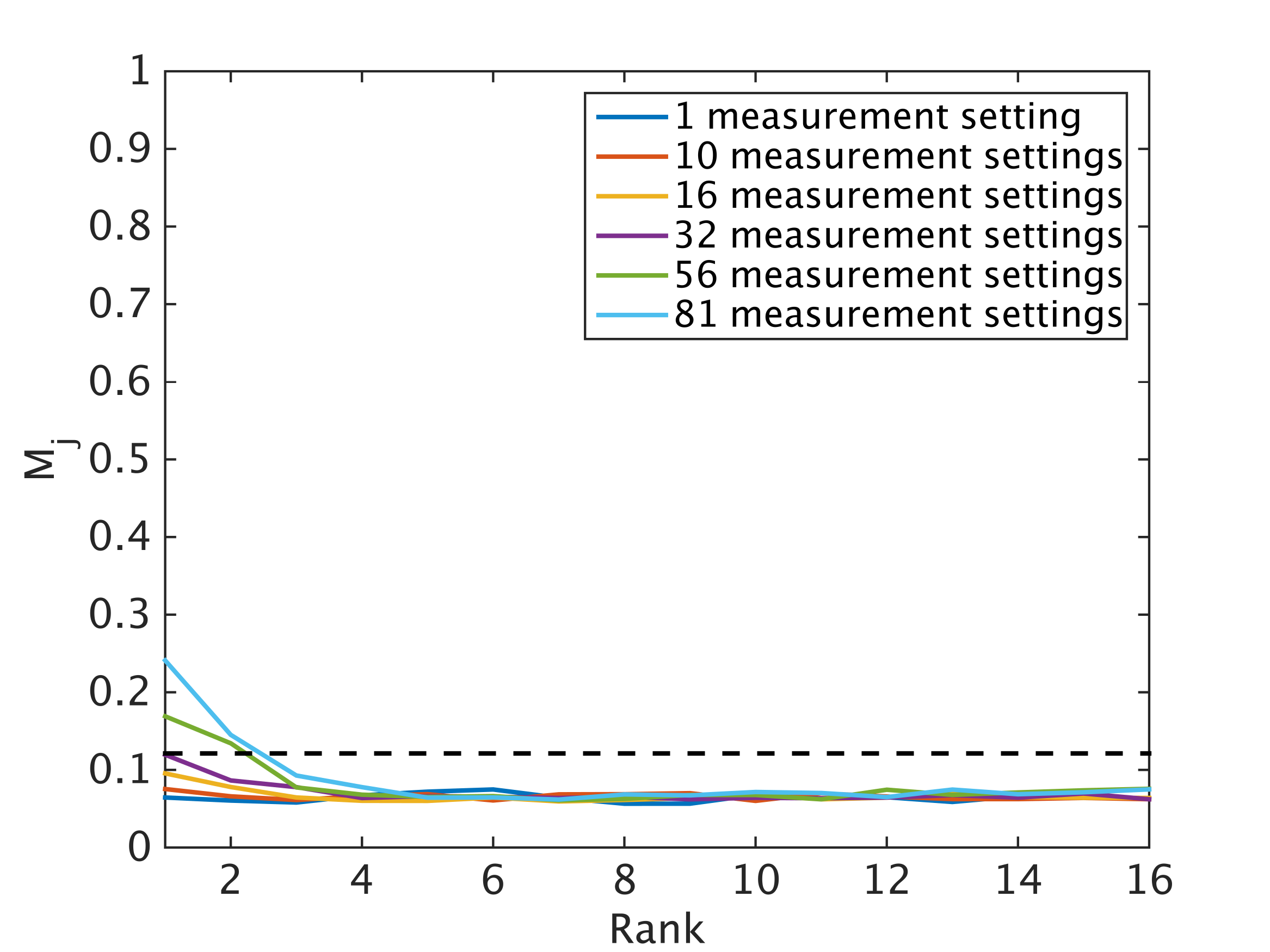
(a)   5 repetitions per measurement setting.

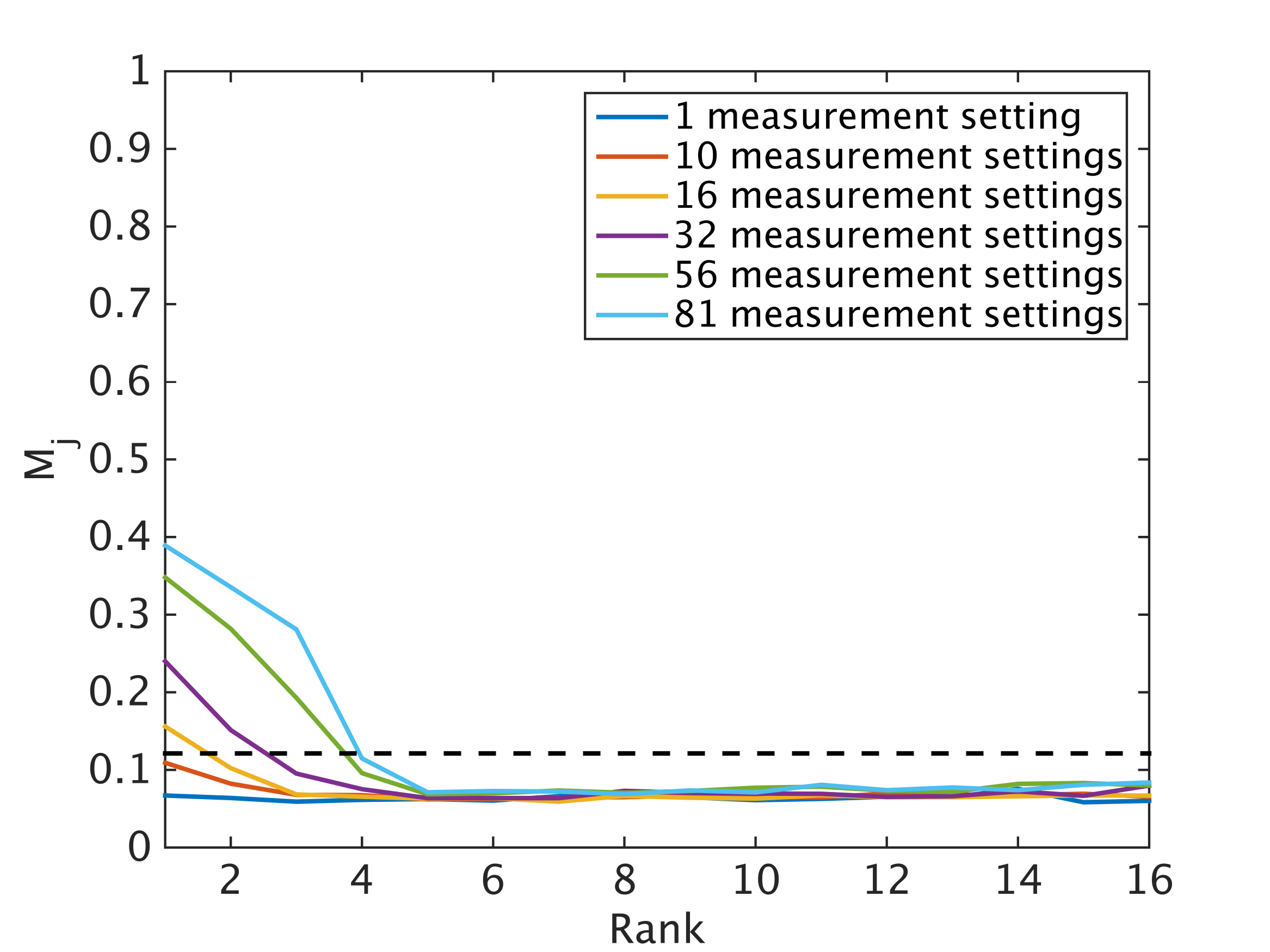
(b)   16 repetitions per measurement setting.

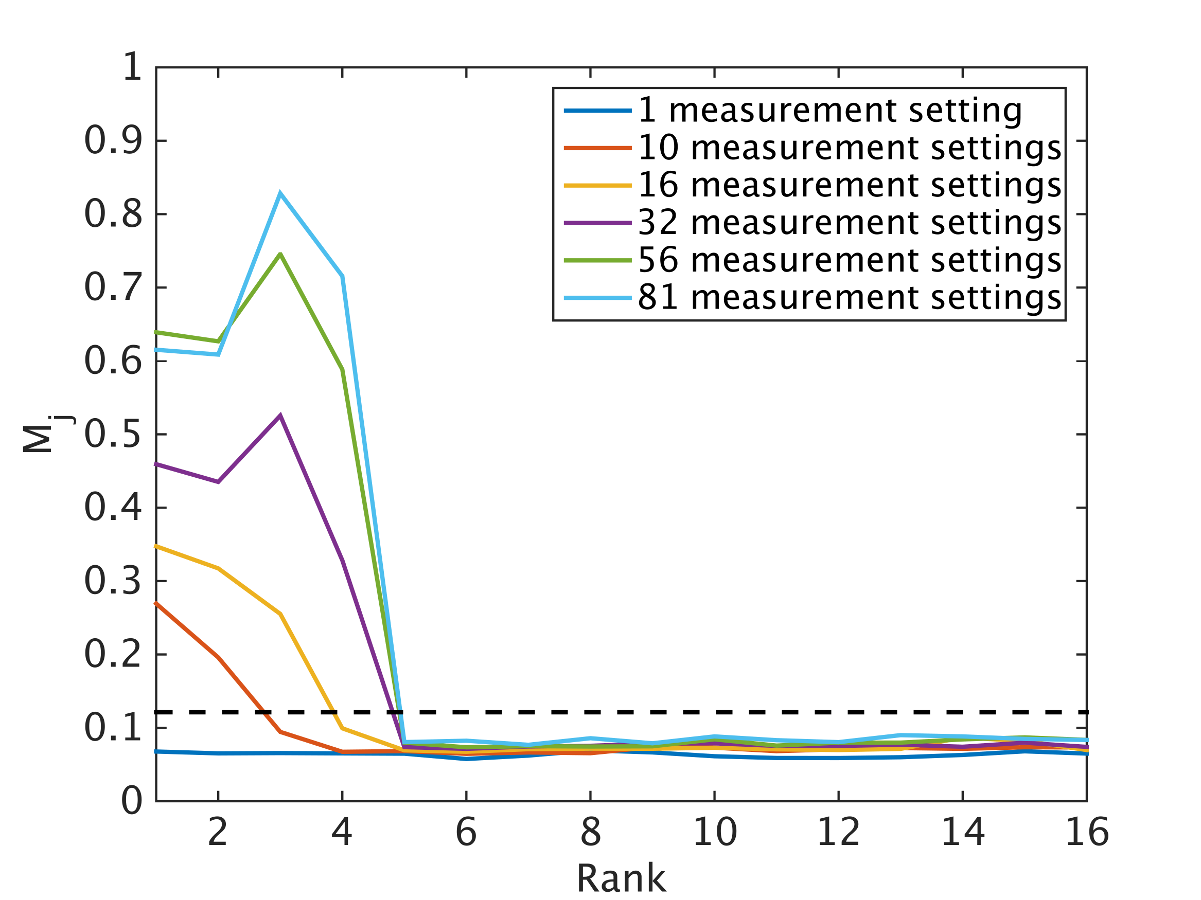
(c)   100 repetitions per measurement setting.

Figure 5: Mean eigenvector overlap as a function of the rank truncation of the recovered density matrix of a true state of rank $4$. The dotted line represents the threshold given in eq. (16).

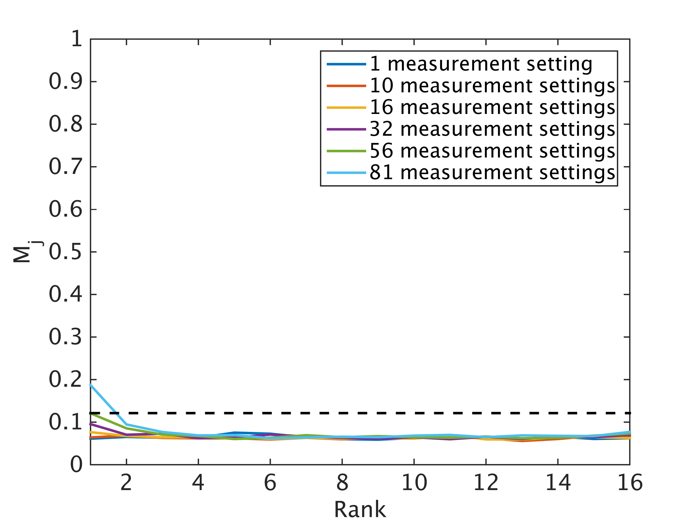
(a)   5 repetitions per measurement setting.

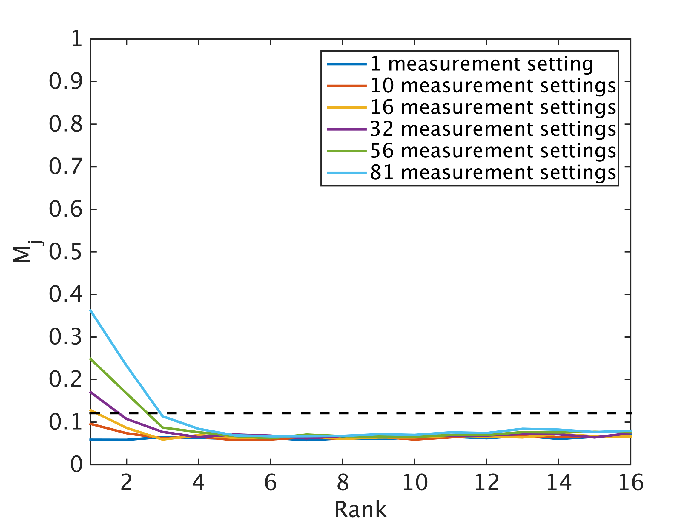
(b)   16 repetitions per measurement setting.

(c)   100 repetitions per measurement setting.

Figure 6: Mean eigenvector overlap as a function of the rank truncation of the recovered density matrix of a true state of rank $8$. The dotted line represents the threshold given in eq. (16).

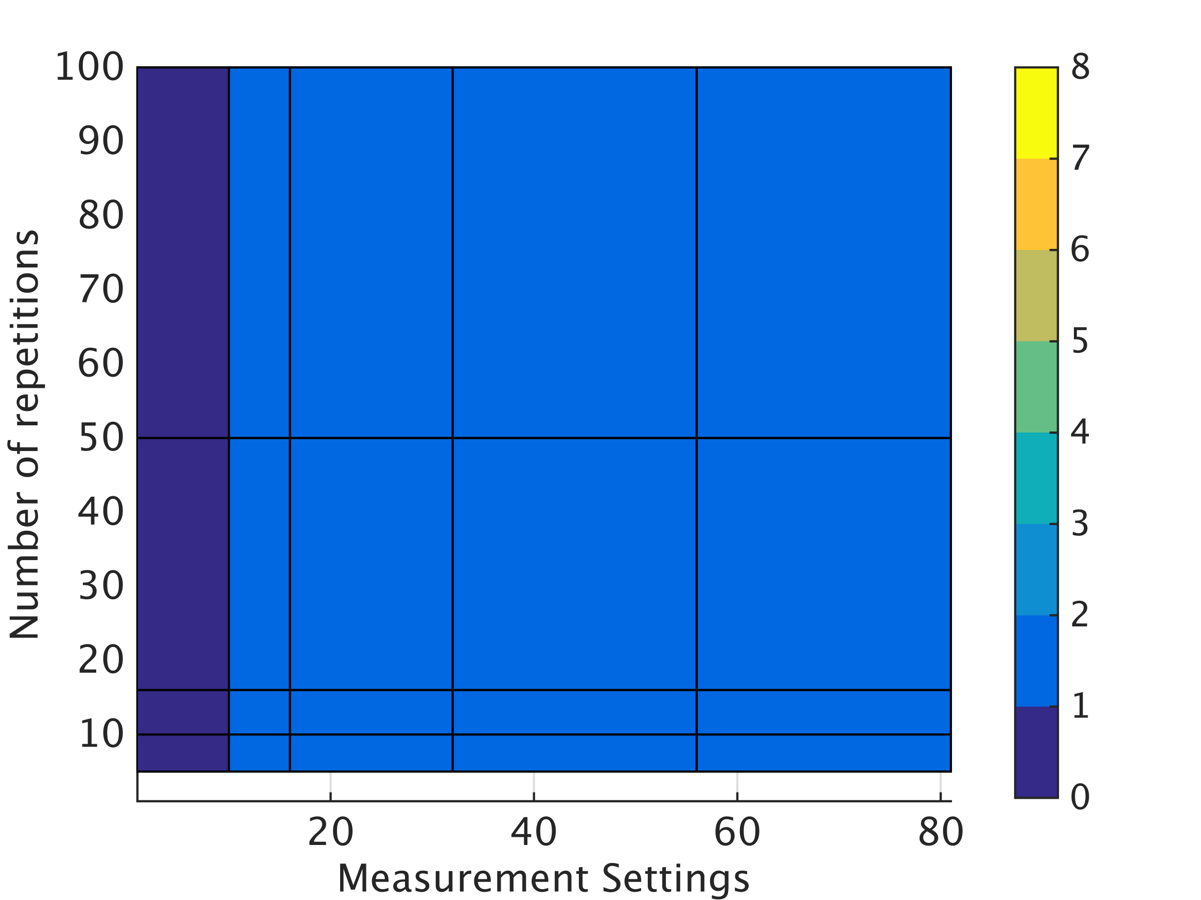
(a)   Rank 1 true state.

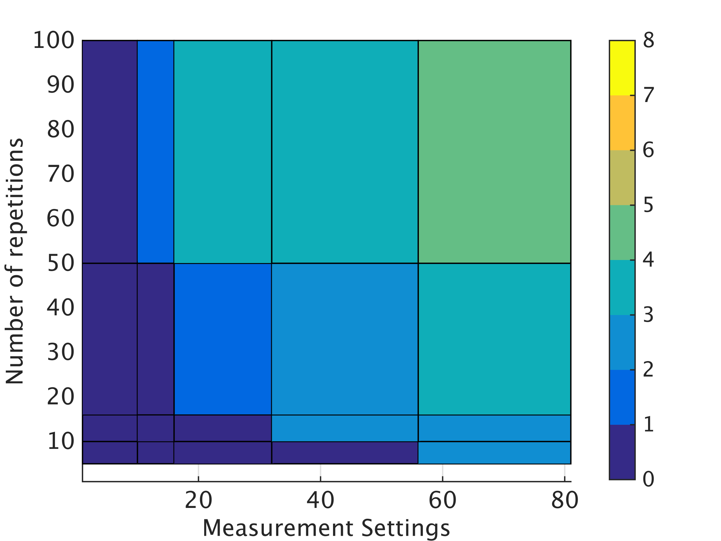
(b)   Rank 4 true state.

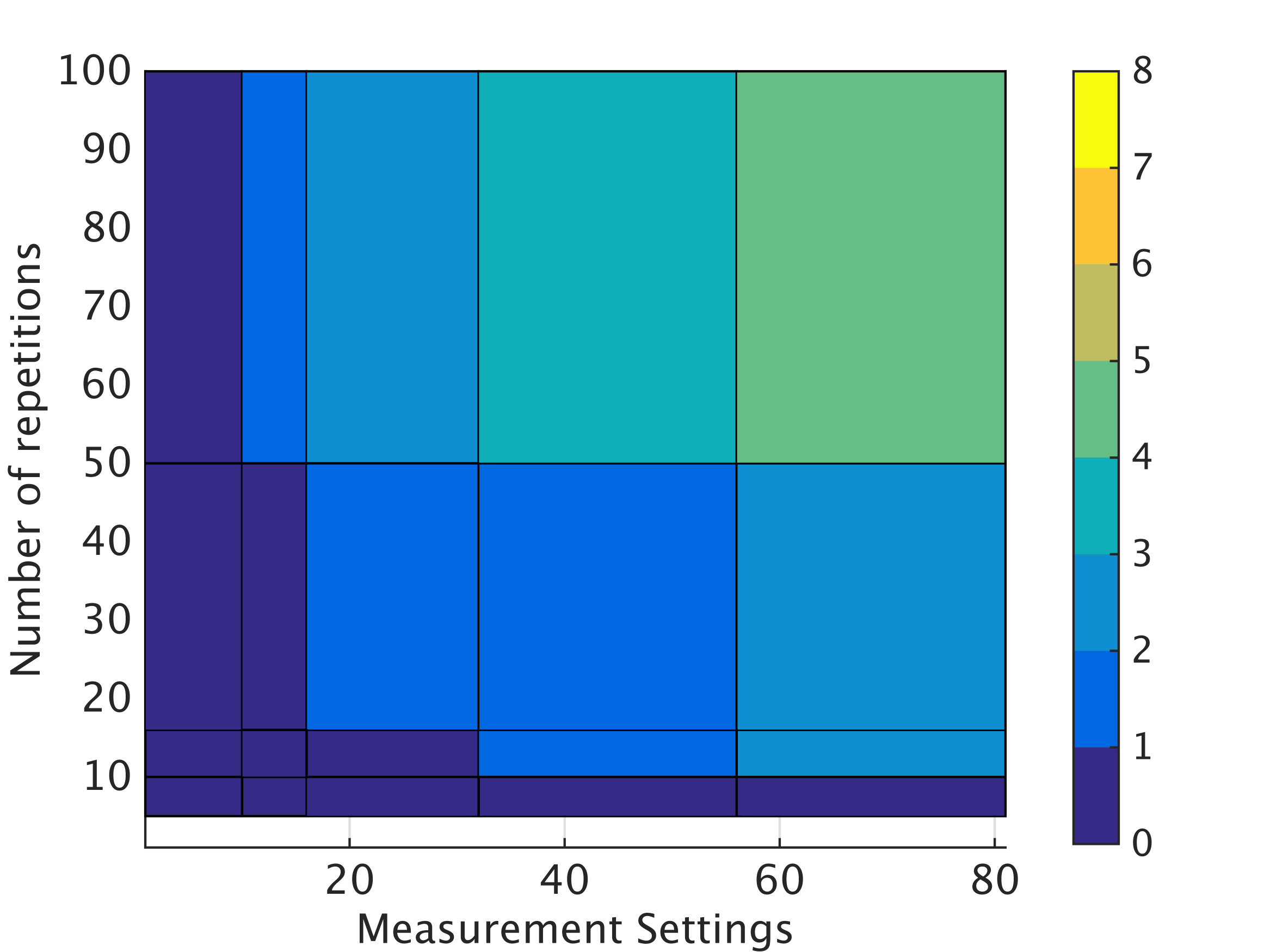
(c)   Rank 8 true state.

Figure 7: Estimated rank according to eq. (15) as a function of the number of measurement settings and number of repetitions per measurement. When insufficient information is available for our criterion to provide a non-zero rank, we choose a rank one estimate by default.

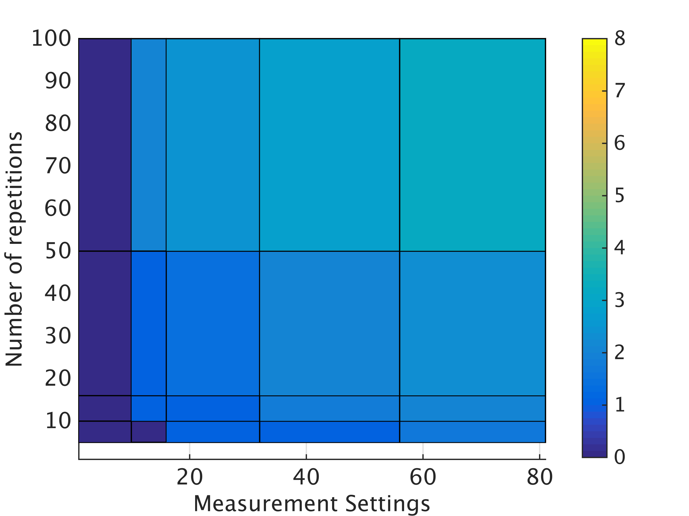
(a)   Rank 1 true state.

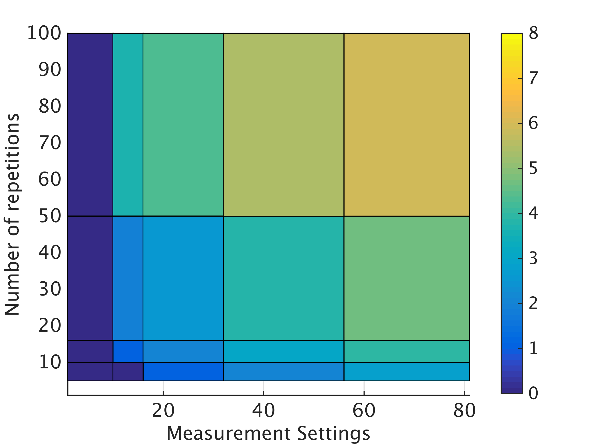
(b)   Rank 4 true state.

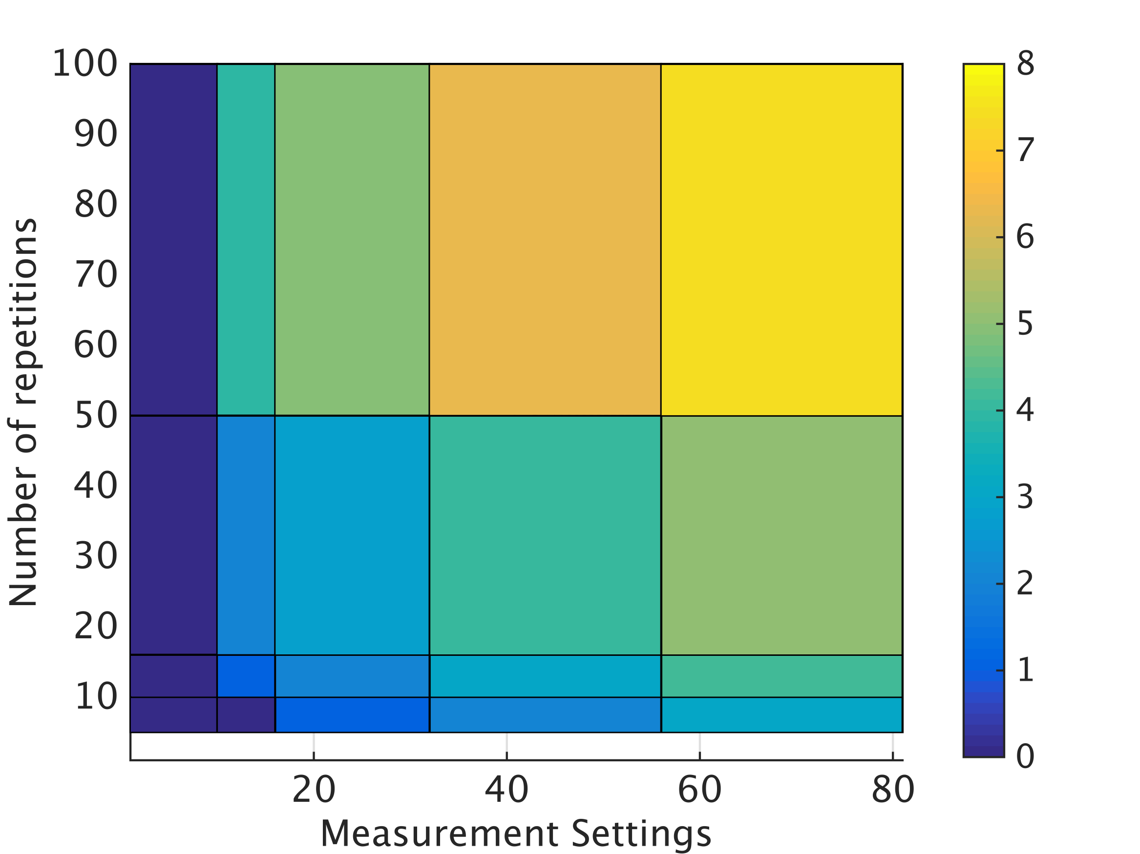
(c)   Rank 8 true state.

Figure 8: Estimated mean rank according to the spectral thresholding method developed in ref. 43 with positivity constraint. The method seems to overfit a little when not enough measurements are used in the reconstruction. Also, note that we are plotting the mean reconstructed rank, which does not take discrete values.

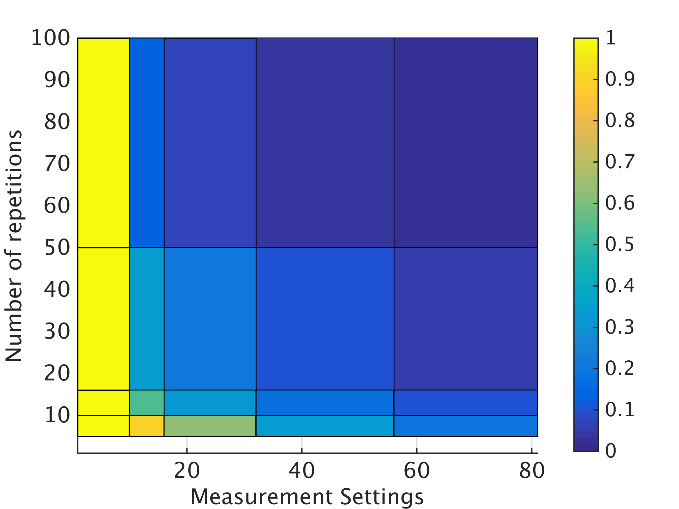
(a)   Rank 1 true state.

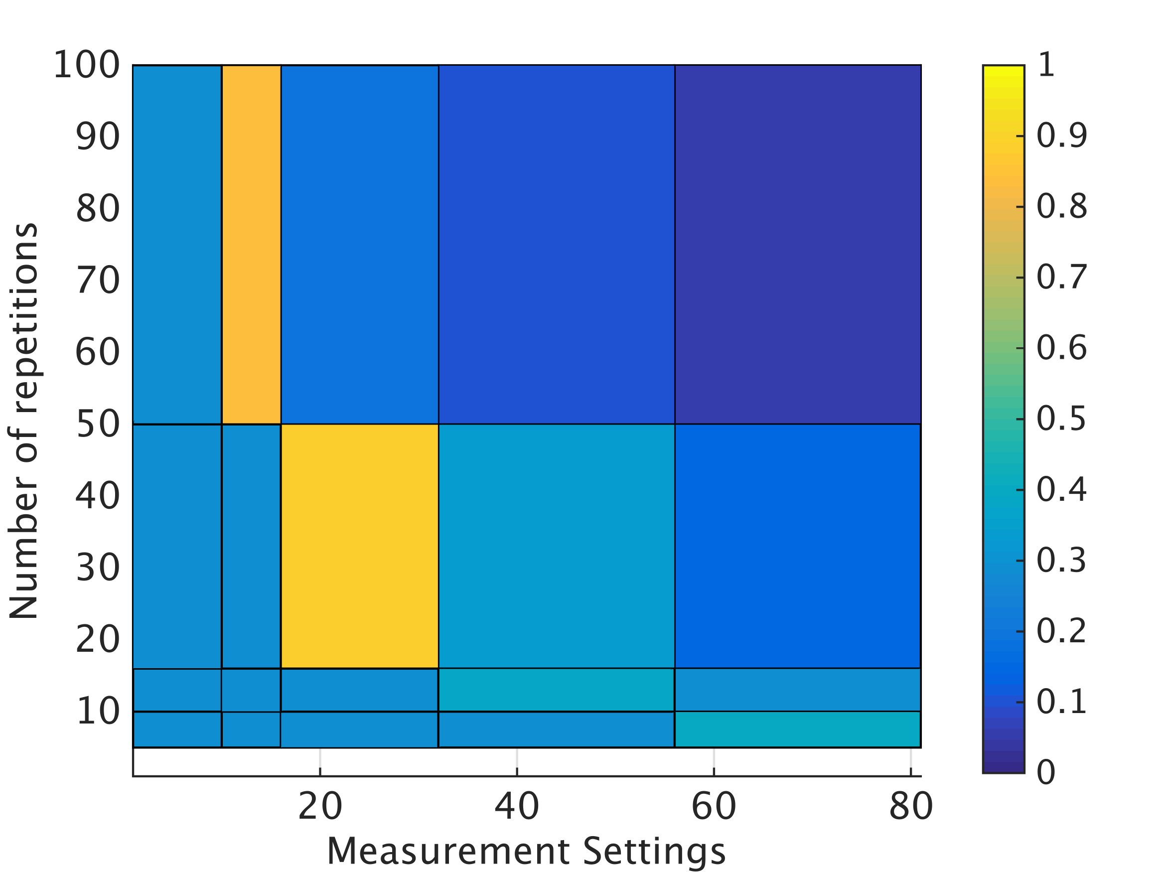
(b)   Rank 4 true state.

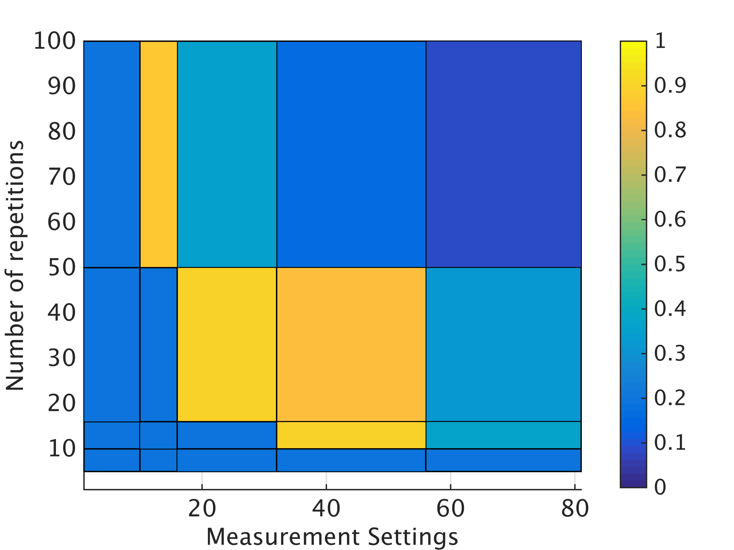
(c)   Rank 8 true state.

Figure 9: Mean risk, eq. (33), computed for the thresholding procedure eq. (15) of the main text.

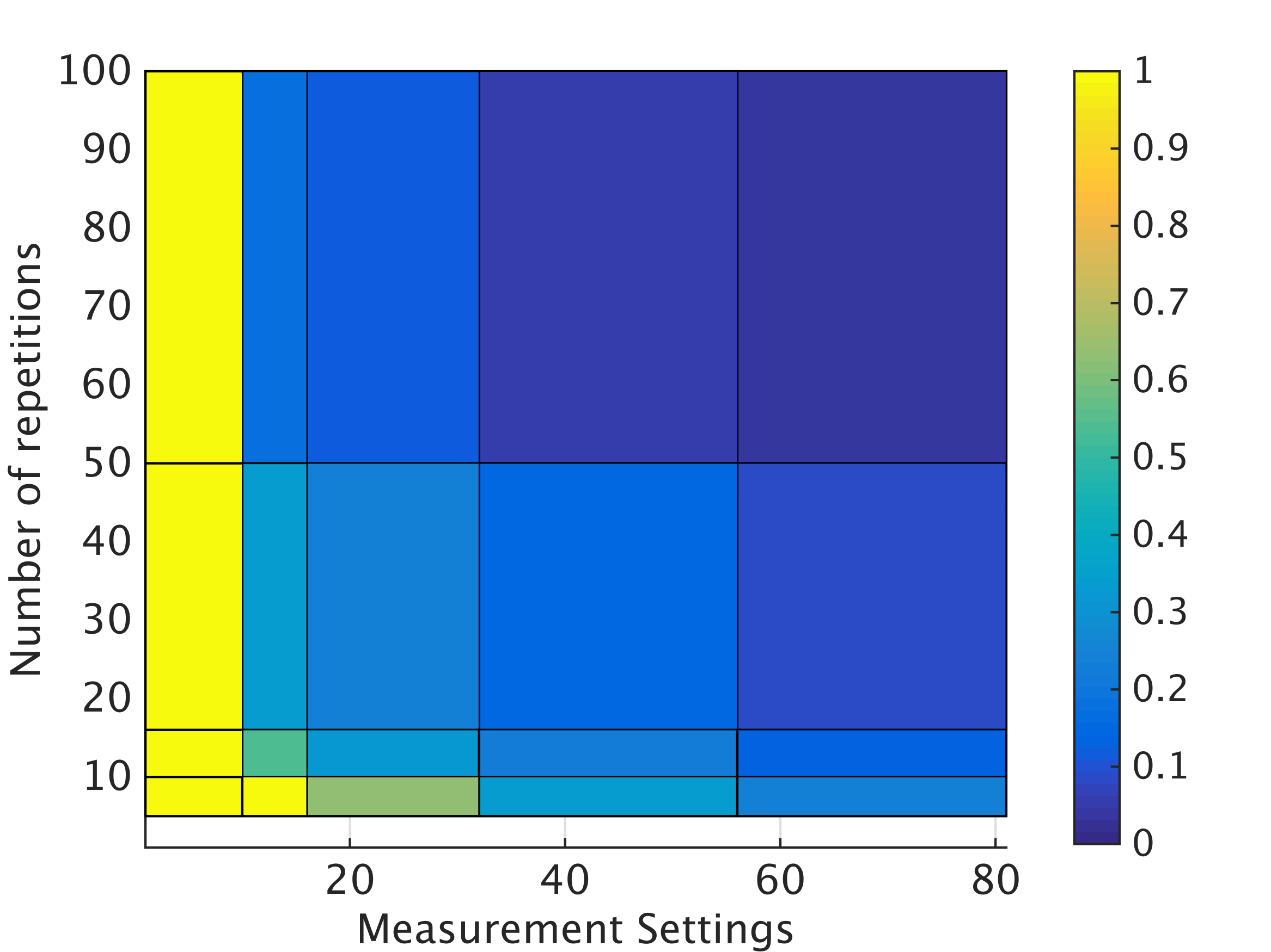
(a)   Rank 1 true state.

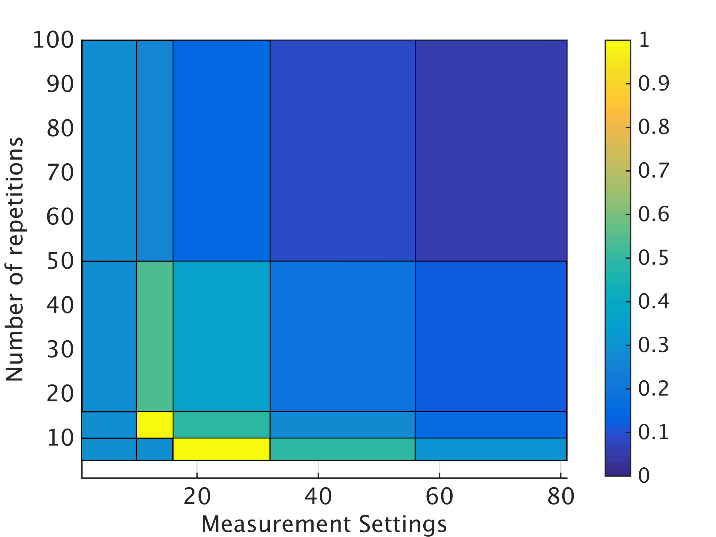
(b)   Rank 4 true state.

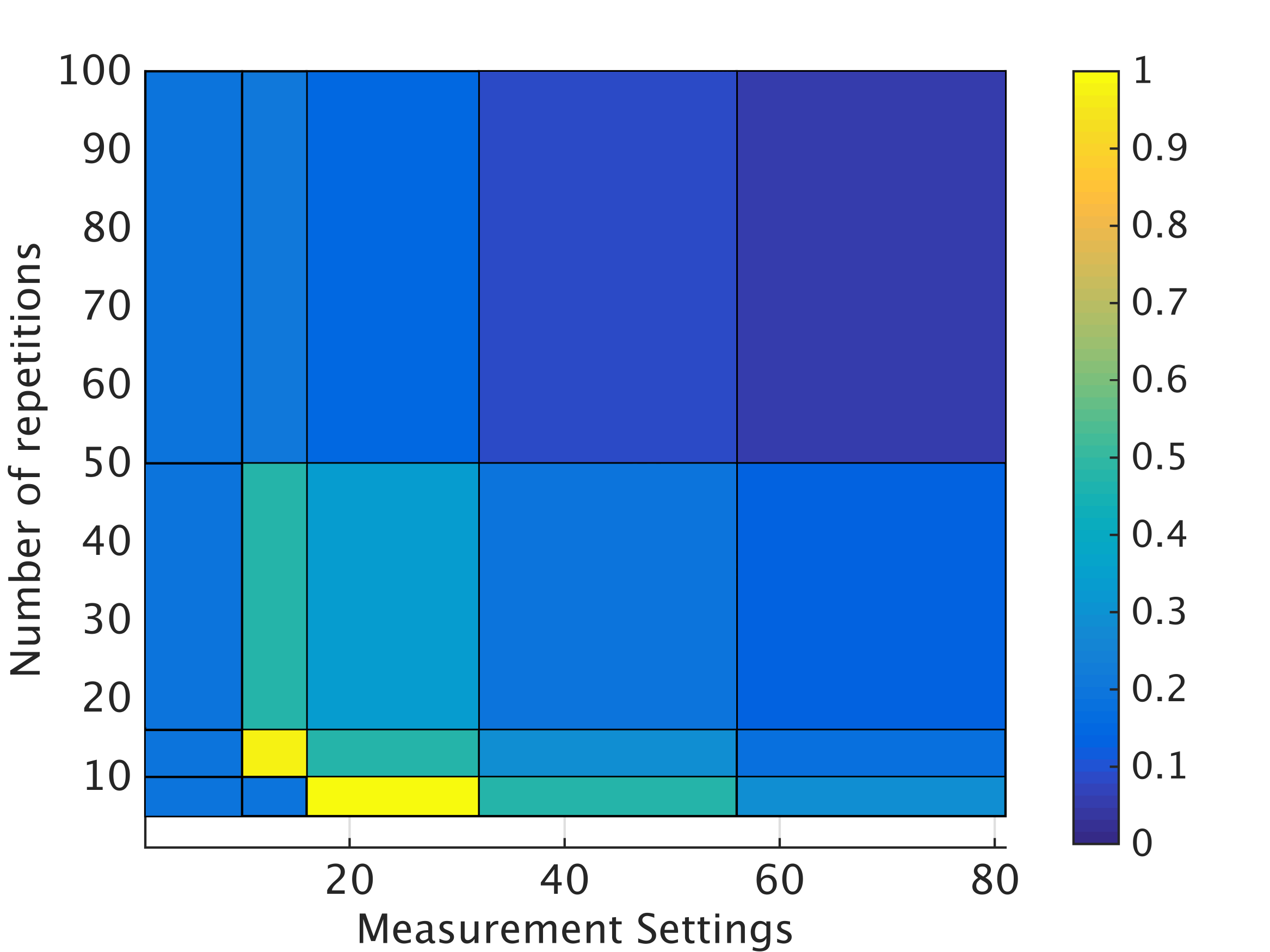
(c)   Rank 8 true state.

Figure 10: Mean risk, eq. (33), computed for the thresholding procedure in ref. 43 with positivity constraint.

Spectral thresholding with experimental data:
Additional results

In this section, we add the results for 2 additional states that were prepared in the laboratory. In figs. 11 and 12 we compare the reconstructed states for the anticipated $|\bar{1}\rangle$ and $(|\bar{0}\rangle+|\bar{1}\rangle)/\sqrt{2}$ encoded state vectors, respectively. As before, we can see how the trace norm minimization can deliver an almost pure state while the least squares estimator does not, which is revealed in the computed fidelities with respect to the anticipated states. Also, note that our spectral thresholding method is also applied successfully.

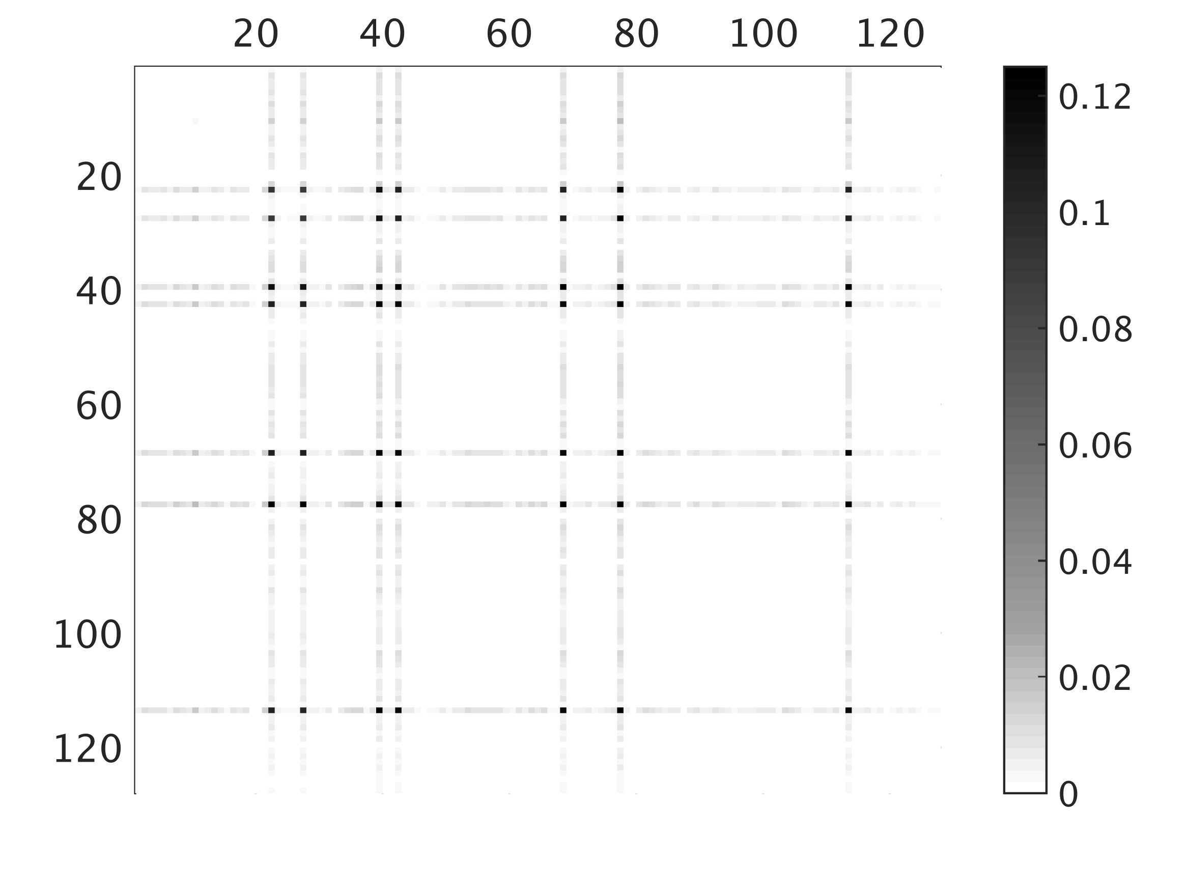
(a)  Trace norm minimization estimate ($F=0.91$), corresponding to the result of the matrix Lasso in eq. (8) in the limit $\mu\rightarrow\infty$.

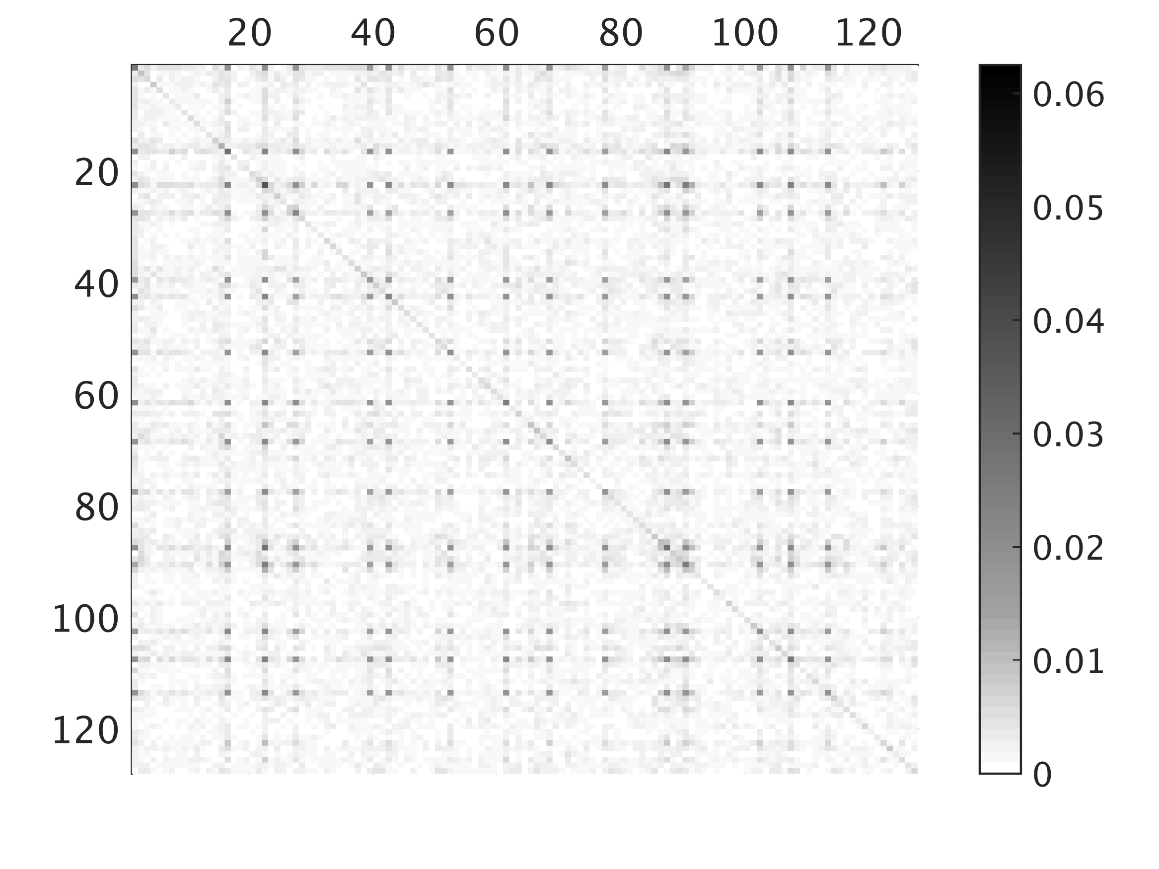
(b)   Least squares estimate ($F=0.23$), corresponding to $\mu=0$.

(c)   Rank $37$ leading subspace projection of the least squares estimate ($F=0.25$) obtained by our spectral thresholding method.

Figure 11: Example of quantum state reconstruction for the logical $|\bar{1}\rangle$ state vector. A 2-D plot of the absolute values of the entries of the density matrix is presented. The same notation as in fig. 1 in the main text is used.

(a)  Trace norm minimization estimate ($F=0.94$), corresponding to the result of the matrix Lasso in eq. (8) in the limit $\mu\rightarrow\infty$.

(b)   Least squares estimate ($F=0.29$), corresponding to $\mu=0$.

(c)   Rank $41$ leading subspace projection of the least squares estimate ($F=0.32$) obtained by our spectral thresholding method.

Figure 12: Example of quantum state reconstruction for the logical $(|\bar{0}\rangle+|\bar{1}\rangle)/\sqrt{2}$ state vector. A 2-D plot of the absolute values of the entries of the density matrix is presented. The same notation as in fig. 1 in the main text is used.

References

- Nigg et al. (2014) D. Nigg, M. Mueller, E. A. Martinez, P. Schindler, M. Hennrich, T. Monz, M. A. Martin-Delgado, and R. Blatt, Science 345, 302 (2014).
- Lanyon et al. (2011) B. P. Lanyon, C. Hempel, D. Nigg, M. Müller, R. Gerritsma, F. Zähringer, P. Schindler, J. T. Barreiro, M. Rambach, G. Kirchmair, M. Hennrich, P. Zoller, R. Blatt, and C. F. Roos, Science 334, 57 (2011).
- Kaufmann et al. (2012) H. Kaufmann, S. Ulm, G. Jacob, U. G. Poschinger, H. Landa, A. Retzker, M. B. Plenio, and F. Schmidt-Kaler, Phys. Rev. Lett. 109, 263003 (2012).
- Blatt and Roos (2012) R. Blatt and C. F. Roos, Nature Phys. 8, 277 (2012).
- Barends et al. (2014) R. Barends, J. Kelly, A. Megrant, A. Veitia, D. Sank, E. Jeffrey, T. C. White, J. Mutus, A. G. Fowler, B. Campbell, Y. Chen, Z. Chen, B. Chiaro, A. Dunsworth, C. Neill, P. O’Malley, P. Roushan, A. Vainsencher, J. Wenner, A. N. Korotkov, A. N. Cleland, and J. M. Martinis, Nature 508, 500 (2014).
- Ofek et al. (2016) N. Ofek, A. Petrenko, R. Heeres, P. Reinhold, Z. Leghtas, B. Vlastakis, Y. Liu, L. Frunzio, S. M. Girvin, L. Jiang, M. Mirrahimi, M. H. Devoret, and R. J. Schoelkopf, (2016), arXiv:1602.04768 .
- Maller et al. (2015) K. M. Maller, M. T. Lichtman, T. Xia, Y. Sun, M. J. Piotrowicz, A. W. Carr, L. Isenhower, and M. Saffman, Phys. Rev. A 92, 022336 (2015).
- Nogrette et al. (2014) F. Nogrette, H. Labuhn, S. Ravets, D. Barredo, L. Béguin, A. Vernier, T. Lahaye, and A. Browaeys, Phys. Rev. X 4, 021034 (2014).
- Lanyon et al. (2013) B. P. Lanyon, P. Jurcevic, M. Zwerger, C. Hempel, E. A. Martinez, W. Dür, H. J. Briegel, R. Blatt, and C. F. Roos, Phys. Rev. Lett. 111, 210501 (2013).
- Vandersypen et al. (2001) L. M. K. Vandersypen, M. Steffen, G. Breyta, C. S. Yannoni, M. H. Sherwood, and I. L. Chuang, Nature 414, 883 (2001).
- Fedorov et al. (2012) A. Fedorov, L. Steffen, M. Baur, M. P. da Silva, and A. Wallraff, Nature 481 (2012).
- Gulde et al. (2003) S. Gulde, M. Riebe, G. P. T. Lancaster, C. Becher, J. Eschner, H. Häffner, F. Schmidt-Kaler, I. L. Chuang, and R. Blatt, Nature 421, 48 (2003).
- Gross et al. (2010) D. Gross, Y.-K. Liu, S. T. Flammia, S. Becker, and J. Eisert, Phys. Rev. Lett. 105, 150401 (2010).
- Cramer et al. (2010) M. Cramer, M. B. Plenio, S. T. Flammia, R. Somma, D. Gross, S. D. Bartlett, O. Landon-Cardinal, D. Poulin, and Y.-K. Liu, Nature Comm. 1, 149 (2010).
- Flammia et al. (2012) S. T. Flammia, D. Gross, Y.-K. Liu, and J. Eisert, New J. Phys. 14, 095022 (2012).
- Flammia and Liu (2011) S. T. Flammia and Y.-K. Liu, Phys. Rev. Lett. 106, 230501 (2011).
- Shabani et al. (2011) A. Shabani, R. L. Kosut, M. Mohseni, H. Rabitz, M. A. Broome, M. P. Almeida, A. Fedrizzi, and A. G. White, Phys. Rev. Lett. 106, 100401 (2011).
- Hübener et al. (2013) R. Hübener, A. Mari, and J. Eisert, Phys. Rev. Lett. 110, 040401 (2013).
- Steffens et al. (2015) A. Steffens, M. Friesdorf, T. Langen, B. Rauer, T. Schweigler, R. Hübener, J. Schmiedmayer, C. A. Riofrio, and J. Eisert, Nature Comm. 6, 7663 (2015).
- Candes and Wakin (2008) E. Candes and M. Wakin, IEEE Signal Process. Mag. 25, 21 (2008).
- Foucart and Rauhut (2013) S. Foucart and H. Rauhut, A mathematical introduction to compressive sensing (Springer, Heidelberg, 2013).
- Eldar (2012) Y. Eldar, Compressed sensing: theory and applications (Cambridge University Press, Cambridge New York, 2012).
- Kueng et al. (2015) R. Kueng, H. Rauhut, and U. Terstiege, Applied and Computational Harmonic Analysis (2015), 10.1016/j.acha.2015.07.007.
- Carpentier et al. (2015) A. Carpentier, J. Eisert, D. Gross, and R. Nickl, arXiv:1504.03234v2 (2015).
- Rodionov et al. (2014) A. V. Rodionov, A. Veitia, R. Barends, J. Kelly, D. Sank, J. Wenner, J. M. Martinis, R. L. Kosut, and A. N. Korotkov, Phys. Rev. B 90, 144504 (2014).
- Schwemmer et al. (2014) C. Schwemmer, G. Toth, A. Niggebaum, T. Moroder, D. Gross, O. Gühne, and H. Weinfurter, Phys. Rev. Lett. 113, 040503 (2014).
- Bombin and Martin-Delgado (2006) H. Bombin and M. A. Martin-Delgado, Phys. Rev. Lett. 97, 180501 (2006).
- Waters et al. (2011) A. E. Waters, A. C. Sankaranarayanan, and R. Baraniuk, in Advances in Neural Information Processing Systems 24, edited by J. Shawe-Taylor, R. S. Zemel, P. L. Bartlett, F. Pereira, and K. Q. Weinberger (Curran Associates, Inc., 2011) pp. 1089–1097.
- Guta et al. (2012) M. Guta, T. Kypraios, and I. Dryden, New J. Phys. 14, 105002 (2012).
- Knips et al. (2015) L. Knips, C. Schwemmer, N. Klein, J. Reuter, G. Tóth, and H. Weinfurter, arXiv:1512.06866v1 (2015).
- Sørensen and Mølmer (1999) A. Sørensen and K. Mølmer, Phys. Rev. Lett. 82, 1971 (1999).
- Schindler et al. (2013) P. Schindler, D. Nigg, T. Monz, J. T. Barreiro, E. Martinez, S. X. Wang, S. Quint, M. F. Brandl, V. Nebendahl, C. F. Roos, M. Chwalla, M. Hennrich, and R. Blatt, New J. Phys. 15, 123012 (2013).
- Calderbank and Shor (1996) A. R. Calderbank and P. W. Shor, Phys. Rev. A 54, 1098 (1996).
- Steane (1996) A. M. Steane, Phys. Rev. Lett. 77, 793 (1996).
- Akaike (1974) H. Akaike, IEEE Trans. Aut. Contr. 19, 716 (1974).
- Aolita et al. (2015) L. Aolita, C. Gogolin, M. Kliesch, and J. Eisert, Nature Comm. 6, 8498 (2015).
- Burer and Monteiro (2003) S. Burer and R. D. C. Monteiro, Math. Program. B 95, 329 (2003).
- Kyrillidis et al. (2012) A. Kyrillidis, S. Becker, V. Cevher, and C. Koch, arXiv:1206.1529 (2012).
- (39) S. Becker, V. Cevher, and A. Kyrillidis, arXiv:1303.0167 .
- Weingarten (1978) D. Weingarten, J. Math. Phys. 19, 999 (1978).
- Suess et al. (2016) D. Suess, L. Rudnicki, and D. Gross, (2016), arXiv:1608.00374.
- Candes (2008) E. J. Candes, Compte Rendus de l’Academie des Sciences 346, 589 (2008).
- Butucea et al. (2015) C. Butucea, M. Guta, and T. Kypraios, (2015), arXiv:1504.08295.