Temperature and interaction dependence of the moment of inertia of a rotating condensate boson gas

Abstract

In this paper, a developed Hartree-Fock semiclassical approximation is used to calculate the temperature and interaction dependence of the moment of inertia of a rotating condensate Boson gas. A fully classical and quantum mechanical treatment for the moment of inertia are given in terms of the normalized temperature. We found that the moment of inertia is considerably affected by the interaction. The present analysis shows that the superfluid effects in the moment of inertia of a condensate Boson gas can be observed at temperatures $T>0.25T_{0}$ and not dramatically smaller than $T_{0}$.

I Introduction

One of the most remarkable characteristics of the Bose-Einstein condensate (BEC) is its response to rotate with superfluid nature Matthews ; Madison ; exp ; Dalibard3 . The superfluid nature of this system is investigated using the moment of inertia. For a macroscopic system, the moment of inertia is given by the rigid value unless it exhibits superfluidity. A deviation of the moment of inertia from the rigid value represents an important manifestion of superfluidity. In this respect, Stringari stringari1 drew a parallel between the rotating BEC and the superfluid systems, and he pointed out that the rotational properties of a BEC provides a natural way to analyze the deviations from a rigid motion due to condensation. Several studies showed that the evidence of the superfluidity in a rotating BEC is the reduction of the moment of inertia below the classical rigid-body value stringari1 ; Brosens ; Schneider ; Odelin ; Zambelli ; Zambelli1 .

Mainly, the moment of inertia is calculated in terms of the effective in situ radii and the normalized temperature. The approach of Brosens et al. Brosens of the moment of inertia is based on the in situ radial radius $\langle x^{2}+y^{2}\rangle$. Their analysis focused on the difference of the moment of inertia of a totally classical Boltzmann gas in a trap and $\langle x^{2}+y^{2}\rangle$ for a Bose gas (cf. Eq. (15)). Therefore, they missed the true superfluid effects that may only be analyzed by calculating the moment of inertia from quantum mechanical response to rotations. In contrast, Stringari’s work stringari1 is based on linear response theory. He obtained the different contributions from the condensate and the thermal cloud to the response coefficient both for an ideal and an interacting Bose gas. Schneider et al. Schneider presented a calculation of the fully quantum mechanical moment of inertia for a microscopic cloud (in the presence of vortices) of non-interacting atoms in a cylindrically symmetrical trap. However, an ideal BEC of (non-interacting bosons) is not a true superfluid, because the Landau criterion for superfluidity is not obeyed Annett . Superfluidity, the formation of the vortex lattice, is a direct effect of inter-particle interactions, that would not occur in the ideal BEC case.

In this work, having clarified that the moment of inertia can be derived in terms of the effective in situ radii, we discuss how quantitative results can be obtained in the presence of interatomic interactions. The temperature-dependent for the in situ radii is calculated within the mean field Hartree-Fock approximation dal ; Sinha ; Sandoval . This approach can be summarized as follow: a conventional method of statistical quantum mechanics is used to calculate the temperature dependency in situ radii. The parametrized formula for the in situ radii are used in calculating the moment of inertia. The obtained results showed that the above mentioned quantities have a special temperature behavior zha .

The paper is planned as follows: section two includes the basic formalism for calculating the effective in situ radii. Interaction and temperature dependency of the moment of inertia are given in section three. Conclusion is given in the last section.

II In situ radii of interacting Bose gas

The ideal Bose-Einstein condensation phenomenon is most conveniently described in the grand-canonical ensemble. For an ideal Bose gas, the average number of particles, $n_{i}$, in a single particle state $|i\rangle$ with energy $\epsilon_{i}$ is given by the familiar Bose-Einstein distribution,

$$n_{i}=\frac{{\textsc{z}}e^{-\beta\epsilon_{i}}}{1-{\textsc{z}}e^{-\beta\epsilon_{i}}}$$ (1)

where $\beta=1/(k_{B}T)$, ${\textsc{z}}=e^{\beta\mu}$ is the effective fugacity, and $\mu$ is the chemical potential, determined by the conservation of total number of particles

$$N=\sum_{i=0}^{\infty}n_{i}=\sum_{i=0}^{\infty}\sum_{j=1}^{\infty}{\textsc{z}}^{j}e^{-j\beta\epsilon_{i}}$$ (2)

The degeneracy factors are avoided by accounting for degenerate states individually. Once z has been determined, all thermodynamically relevant quantities can be calculated from partial derivatives of the grand potential $q$, the logarithm of the grand canonical partition function, such as the in situ radii, the condensate fraction, etc.

The effective in situ radius of trapped ideal boson gas was obtained by considering the statistical quantum mechanics arguments zha ; bra . For a trapped boson in spherically symmetric harmonic potential, $V(r)=m\omega^{2}r^{2}/2$, the effective in situ radius of a single particle state $|i\rangle$ is given by its expectation value in this stat,i.e.

$$\langle r_{i}^{2}\rangle=\frac{\epsilon_{i}}{m\omega^{2}}$$ (3)

with $\epsilon_{i}=\hbar\omega(i+\frac{3}{2})$ is the eigenvalue of the potential $V(\bf r)$. The effective in situ radius of $N$ atoms is found by gathering Eqs.(2) and (3)

$$N\langle r_{i}^{2}\rangle = \frac{1}{m\omega^{2}}\ \sum_{i=0}^{\infty}\epsilon_{i}\sum_{j=1}^{\infty}{\textsc{z}}^{j}e^{-j\beta\epsilon_{i}}$$ (4)

$$= -\frac{1}{m\omega^{2}}\frac{\partial}{\partial\beta}\sum_{i=0}^{\infty}\sum_{j=1}^{\infty}\frac{{\textsc{z}}^{j}}{j}e^{-j\beta\epsilon_{i}}$$

and can be expressed in terms of the thermodynamic potential $q$,

$$q = -\sum_{i=0}^{\infty}\ln(1-{\textsc{z}}e^{-\beta\epsilon_{i}})=\sum_{i=0}^{\infty}\sum_{j=1}^{\infty}\frac{{\textsc{z}}^{j}}{j}e^{-j\beta\epsilon_{i}}$$ (5)

the relation $\ln(1-y)=-\sum_{j=1}^{\infty}\frac{y^{j}}{j}$ is used here. Thus the effective in situ radius is given by

$$\langle r^{2}\rangle=-\frac{1}{m\omega^{2}}\frac{\partial q}{\partial\beta}$$ (6)

For a cylindrically symmetric trap with $\omega_{x}=\omega_{y}=\omega_{\bot}$, the temperature dependence of the three effective in situ is the same as in a spherically symmetric trap discussed above. Assuming an axial trap frequency $\omega_{z}=\lambda\omega_{\bot}$.

$$N{\langle x^{2}\rangle} = -\frac{1}{3}\lambda^{1/3}\frac{1}{m\omega_{x}^{2}}\frac{\partial q}{\partial\beta}$$

$$N{\langle y^{2}\rangle} = -\frac{1}{3}\lambda^{1/3}\frac{1}{m\omega_{y}^{2}}\frac{\partial q}{\partial\beta}$$

$$N{\langle z^{2}\rangle} = -\frac{1}{3}\lambda^{-2/3}\frac{1}{m\omega_{z}^{2}}\frac{\partial q}{\partial\beta}$$ (7)

where $\lambda$ is the trap deformation parameter. Generalization to highly anisotropic trap (which is mainly used for rotating condensate) is straightforward. Assuming that the trap deformation parameters for highly anisotropic trap are given by

$$\lambda_{x}=\frac{\omega_{z}}{\omega_{x}},\lambda_{y}=\frac{\omega_{z}}{\omega_{y}}$$

the three effective in situ radii are given by zha ; ahm1 ,

$$N{\langle x^{2}\rangle} = -\frac{1}{3}\big{(}\frac{\lambda_{x}^{2}}{\lambda_{y}}\big{)}^{1/3}\frac{1}{m\omega_{x}^{2}}\frac{\partial q}{\partial\beta}$$

$$N{\langle y^{2}\rangle} = -\frac{1}{3}\big{(}\frac{\lambda_{y}^{2}}{\lambda_{x}}\big{)}^{1/3}\frac{1}{m\omega_{y}^{2}}\frac{\partial q}{\partial\beta}$$

$$N{\langle z^{2}\rangle} = -\frac{1}{3}\big{(}\frac{1}{\lambda_{x}\lambda_{y}}\big{)}^{1/3}\frac{1}{m\omega_{z}^{2}}\frac{\partial q}{\partial\beta}$$ (8)

However, once the thermodynamic potential $q$ has been determined, the effective in situ radius can be calculated. our approach is expected to provide correctly the interaction dependence of $q$ potential, apart from the critical behavior near the BEC transition temperature where the mean-field approach is known to fail.

Generally, the simplest way to include the interaction effect is to use the Hartree-Fock approximation. Within this approximation, the thermal component is treated as a gas of non-interacting atoms moving in a self-consistently determined mean-field potential given by

$$V_{eff}(x,y,z)=V_{trap}(x,y,z)+2g[n_{th}(x,y,z)+n_{0}(x,y,z)],$$ (9)

where $g=\frac{4\pi\hbar^{2}a}{m}$ is the interaction strength and

$$V_{trap}(x,y,z)=\frac{1}{2}m[\omega_{x}^{2}x^{2}+\omega_{y}^{2}y^{2}+\omega_{z}^{2}z^{2}],$$ (10)

with $\{\omega_{x},\omega_{y},\omega_{z}\}$ are the effective trapping frequencies. The densities of the thermal and condensate component are given as a solution of the two coupled equations: the thermal atoms satisfies Schrödinger equation

$$\Big{[}\frac{p_{x}^{2}+p_{y}^{2}+p_{z}^{2}}{2m}+V_{eff}(x,y,z)\Big{]}\psi_{i}(x,y,z)=\epsilon_{i}\psi_{i}(x,y,z)$$ (11)

while the condensate part satisfies the time independent Gross-Pitaevskii equation

$$\Big{[}\frac{p_{x}^{2}+p_{y}^{2}+p_{z}^{2}}{2m}+V_{eff}(x,y,z)-gn_{0}(x,y,z)\Big{]}\phi(x,y,z)=\mu\phi(x,y,z),$$ (12)

Equations (11) and (12) along with the constraint that the total number of atoms $N$ is fixed,

$$N=\int n_{th}{(x,y,z)}dxdydz+\int n_{0}{(x,y,z)}dxdydz$$ (13)

form a closed set of equations which should be solved self-consistently. Two further simplifications can be made as a consequence of the relative diluteness of the thermal component compared to the condensate Campbell :
(i) at very low temperature the effect of thermal atoms on the condensate can be neglected. Therefore, setting $n_{th}(x,y,z)\approx 0$ in Eq.(12) and applying the Thomas-Fermi (TF) approximation gives the usual TF profile for the condensate

$$n_{0}(x,y,z)=\frac{\mu-V_{trap}(x,y,z)}{g}$$ (14)

For all $\mu>V_{trap}(x,y,z)$ and $n_{0}(x,y,z)$ = 0 elsewhere. Substituting from Eq.(10) in Eq.(14) leads to,

$$n_{0}(x,y,z)=\frac{\mu}{g}\Big{[}1-\frac{x^{2}}{R_{x}^{2}(\mu)}-\frac{y^{2}}{R_{y}^{2}(\mu)}-\frac{z^{2}}{R_{z}^{2}(\mu)}\Big{]}$$ (15)

where $R_{\alpha}(\mu)=\sqrt{\frac{2\mu}{m\omega_{\alpha}^{2}}}$ is the Thomas-Fermi radius at which the condensate density drops to zero along the $x,y$ or $z$ axis. The result in Eq.(15) can be expressed in terms of the condensate number of atoms through the relation between $\mu$ and $N_{0}$,

$$N_{0} = \int n_{0}(x,y,z)dxdydz$$ (16)

$$= \frac{8\pi}{15}\frac{\mu}{g}(R_{x}R_{y}R_{z})=\frac{8\pi}{15}\frac{\mu}{g}{\bar{R}}^{3}$$

$\bar{R}$ representing the geometric mean $(R_{x}R_{y}R_{z})^{1/3}$. Equation (16) can be inverted to give ${\mu}$ in terms of $N_{0}$ such that,

$$\mu = \frac{1}{2}\hbar\omega_{g}\Big{(}\frac{15N_{0}a}{a_{har}}\big{)}^{2/5}$$ (17)

where $a$ is the s-wave scattering length, $a_{har}=\sqrt{\hbar/m\omega_{g}}$ and $\omega_{g}=(\omega_{x}\omega_{y}\omega_{z})^{1/3}$.
(ii) further, within the same approximation, the mean-field energy, $2gn_{th}(x,y,z)$ due to the thermal component itself can be neglected, so that the effective potential experienced by the thermal atoms is then given by

$$V_{eff}(x,y,z) = V_{trap}(x,y,z)+2gn_{0}(x,y,z),$$ (18)

$$= |V_{trap}(x,y,z)-\mu_{0}|+\mu_{0}$$

where the mean-field chemical potential $\mu_{0}$ is given by Eq.(17) and $T\to 0$ limit is indicated. Eq.(18) shows that the condensate density is drastically altered from the ideal case, reflecting that the shape of the confining potential has a three-dimensional ‘Mexican-hat’ shape bretin . Moreover, $\mu_{0}$ is the relevant energy scale parametrizing the effects of interactions, up to the point in the trap where $\mu_{0}=V_{trap}(x,y,z)$.

Now, it is straightforward to calculate the thermodynamic potential $q$ for the interacting Bose gas Sinha ; hau . However, for large number of particles in the system, Eq.(5) provides a complicated sum over $i$. It is hard to evaluate this sum analytically in a closed form. Another possible way to do this analysis, is to use the semiclassical approximation in which the sum in Eq.(5) is converted into a phase space integral Sinha ; hau ,

$$q = q_{0}+\frac{1}{(2\pi\hbar)^{3}}\sum_{j=1}^{\infty}\frac{{\textsc{z}}^{j}}{j}\int e^{-j\beta[\frac{p_{x}^{2}+p_{y}^{2}+p_{z}^{2}}{2m}+V_{eff}(x,y,z)]}{dp_{x}dp_{y}dp_{z}dxdydz}$$ (19)

$$= q_{0}+\frac{1}{\lambda_{th}^{3}}\sum_{j=1}^{\infty}\frac{{\textsc{z}}^{j}}{j^{5/2}}\int e^{-j\beta V_{eff}(x,y,z)}{dxdydz}$$

where $q_{0}=-\ln(1-{\textsc{z}})$ is the thermodynamic potential accounted for the atoms in the ground state and $\lambda_{th}=\sqrt{\frac{2\pi\hbar^{2}}{mk_{B}T}}$ is the thermal de Broglie wavelength. The second term in Eq.(19) provides the thermodynamic potential for the thermal atoms.

In order to calculate the above integral (19), we followed the Hadzibabic and co-worker tammuz ; Campbell approach’s and consider the same approximation. For relatively high temperature, (compared with $\mu_{0}/k_{B}$) the majority of thermal atoms lie outside the condensate in the region where $V_{eff}(x,y,z)>\mu_{0}$ and $V_{eff}(x,y,z)=V_{trap}(x,y,z)$. Therefore, it is reasonable to approximate the full effective potential as the bare trapping potential and consider only the region outside the condensate. This does not mean that the effect of interactions may be neglected as the chemical potential has a value that differs substantially from the ideal value. Therefore Eq.(19) becomes

$$q = q_{0}+\frac{1}{\lambda_{th}^{3}}\sum_{j=1}^{\infty}\frac{1}{j^{5/2}}\int e^{-j\beta[V_{trap}(x,y,z)-\mu_{0}]}dxdydz$$ (20)

Note that in deriving this equation we used ${\textsc{z}}^{j}=e^{j\beta\mu_{0}}$. Substituting the harmonic form of $V_{trap}(x,y,z)$ into Eq.(20) gives

$$q = q_{0}+\frac{1}{\lambda_{th}^{3}}\sum_{j=1}^{\infty}\frac{{1}}{j^{5/2}}\int e^{-j\beta[\frac{1}{2}m(\omega_{x}^{2}x^{2}+\omega_{y}^{2}y^{2}+\omega_{z}^{2}z^{2})-\mu_{0}]}$$ (21)

Introducing the thermal radius, which fixed the maximum value of the chemical potential compared to $k_{B}T$,

$$R_{\alpha}^{\prime}(T)=\sqrt{\frac{2}{\beta m\omega_{\alpha}^{2}}}$$ (22)

these radius is equivalent to the condensate Thomas-Fermi radius at which the thermal density drops to zero along $T\to 0$. In terms of $R_{\alpha}^{\prime}(T)$ Eq.(21) becomes,

$$q = q_{0}+\frac{1}{\lambda_{th}^{3}}\sum_{j=1}^{\infty}\frac{1}{j^{5/2}}\int e^{-j\big{(}\frac{x^{2}}{{R_{x}^{\prime}}^{2}}+\frac{y^{2}}{{R_{y}^{\prime}}^{2}}+\frac{{z}^{2}}{{R_{z}^{\prime}}^{2}}-\alpha_{0}\big{)}}dxdydz$$ (23)

$$= q_{0}+4\pi\frac{{R_{x}^{\prime}R_{y}^{\prime}}R_{z}^{\prime}}{\lambda_{th}^{3}}\sum_{j=1}^{\infty}\frac{1}{j^{5/2}}\int_{\sqrt{\alpha_{0}}}^{\infty}R^{2}e^{-j(R^{2}-\alpha_{0})}dR$$

where the factor $4\pi$ is due to the integration over the angles and

$$\alpha_{0} = {\mu_{0}\beta},\ \ R^{2}=\frac{x^{2}}{{R_{x}^{\prime}}^{2}}+\frac{y^{2}}{{R_{y}^{\prime}}^{2}}+\frac{{z}^{2}}{{R_{z}^{\prime}}^{2}},$$ (24)

it is sensible to introduce the variable $Q$, where

$${Q^{2}}={R^{2}}-\alpha_{0}$$ (25)

to rewrite (23) as

$$q = q_{0}+4\pi\frac{{R_{x}^{\prime}R_{y}^{\prime}}R_{z}^{\prime}}{\lambda_{th}^{3}}\sum_{j=1}^{\infty}\frac{1}{j^{5/2}}\int_{0}^{\infty}Q^{2}\Big{(}1+\frac{\alpha_{0}}{Q^{2}}\Big{)}^{\frac{1}{2}}e^{-j\frac{Q^{2}}{2}}dQ$$

$$= q_{0}+4\pi\frac{{R_{x}^{\prime}R_{y}^{\prime}}R_{z}^{\prime}}{\lambda_{th}^{3}}\sum_{j=1}^{\infty}\frac{1}{j^{5/2}}\int_{0}^{\infty}(Q^{2}+\frac{\alpha_{0}}{2})e^{-j{Q^{2}}}dQ$$

where the binomial expansion has been evaluated to first order in $\alpha_{0}$ . Evaluating the Gaussian integral in (LABEL:eq106) and used $\zeta(s)=\sum_{j=1}^{\infty}\frac{1}{j^{s}}$ leads to

$$q = q_{0}+4\pi\frac{R_{x}^{\prime}R_{y}^{\prime}R_{z}^{\prime}}{\lambda_{th}^{3}}\sum_{j=1}^{\infty}\frac{1}{j^{5/2}}\Big{(}\frac{\sqrt{\pi}/4}{j^{3/2}}+\frac{\sqrt{\pi}/4}{j^{1/2}}\ \alpha_{0}\Big{)}$$ (27)

$$= q_{0}+\Big{(}\frac{1}{\beta\hbar\omega_{g}}\Big{)}^{3}\big{[}\zeta(4)+{\beta\mu_{0}}\zeta(3)\big{]}$$

where $\omega_{g}=(\omega_{x}\omega_{y}\omega_{z})^{1/3}$ for highly anisotropic trap. Expressions for other trap type (cylindrically or spherically) can be extracted from Eq.(16) by setting the trap frequencies. Direct comparison between this results and the $q$ potential for the ideal system pat ,

$$q^{id}=q_{0}^{id}+\Big{(}\frac{1}{\beta\hbar\omega_{g}}\Big{)}^{3}g_{4}({\textsc{z}})$$ (28)

shows that the first and the second terms in Eq.(27) are in comparable with the result of the ideal system at $T<T_{0}$ with $T_{0}=\frac{\hbar\omega_{g}}{k_{B}}\big{(}\frac{N}{\zeta(3)}\big{)}^{1/3}$ is the BEC transition temperature for the non-interacting gas and $\zeta$ is the Riemann zeta function and $g_{\nu}(\textsc{z})=\sum_{k=1}^{\infty}{{\textsc{z}}}^{k}/k^{\nu}$ is the usual Bose function. The last term in Eq.(27) accounted well for the interaction effect. This effect can be seen more clearly by using Stringari et al. dal ; strin interaction scaling parameter $\eta$. This parameter is determined by the ratio between the chemical potential at $T=0$ value calculated in Thomas-Fermi approximation, $\mu_{0}$ and the transition temperature for the non-interacting particles in the same trap, i.e. $\eta=\frac{\mu_{0}}{K_{B}T_{0}}$ (the typical values for $\eta$ for most experiments ranges from 0.30 to 0.40.).

Finally, we reach to the main results of our work. The interaction dependence for the  in situ radius for the spherically symmetric trap can be obtained by substituting from Eq.(27), after setting $\omega_{x}=\omega_{y}=\omega_{z}=\omega$, into Eq.(4), i.e.

$$N\langle r_{i}^{2}\rangle = -\frac{1}{m\omega^{2}}\frac{\partial q}{\partial\beta}$$ (29)

$$= -\frac{1}{m\omega^{2}}\frac{\partial}{\partial\beta}\big{[}-\ln(1-{\textsc{z}})+\Big{(}\frac{1}{\beta\hbar\omega}\Big{)}^{3}[\zeta(4)+{\beta\mu_{0}}\zeta(3)]\big{]}$$

$$= -\frac{1}{m\omega^{2}}\big{[}\frac{-1}{1-{\textsc{z}}}\frac{\partial{\textsc{z}}}{\partial\beta}-\Big{(}\frac{1}{\hbar\omega}\Big{)}^{3}[3\frac{\zeta(4)}{\beta^{4}}+2\mu_{0}\frac{\zeta(3)}{\beta^{3}}]\big{]}$$

$$= \frac{\mu_{0}}{m\omega^{2}}N_{0}(T)+3\Big{(}\frac{k_{B}T}{m\omega^{2}}\Big{)}[\zeta(4)+\frac{2}{3}\frac{\mu_{0}}{k_{B}T}\zeta(3)]\Big{(}\frac{k_{B}T}{\hbar\omega}\Big{)}^{3}$$

$$= \frac{\mu_{0}}{m\omega^{2}}N_{0}(T)+3\Big{(}\frac{k_{B}T}{m\omega^{2}}\Big{)}\big{[}\frac{\zeta(4)}{g_{3}({\textsc{z}})}+\frac{2}{3}\frac{\mu_{0}}{k_{B}T}\frac{\zeta(3)}{g_{3}({\textsc{z}})}\big{]}(N-N_{0}(T))$$

where $q_{0}=-\ln(1-{\textsc{z}}),{\textsc{z}}=e^{\beta\mu}$ and $N_{0}(T)=\frac{{\textsc{z}}}{1-{\textsc{z}}}$ are used here.

The generalization of the above treatment to a trap with three different frequencies, ($\omega_{x},\omega_{y}$ and $\omega_{z}$ ) is straightforward. Substituting from Eq.(27) into Eq.(8) leads to,

$$N\langle x^{2}\rangle=\big{(}\frac{\lambda_{x}^{2}}{\lambda_{y}}\big{)}^{1/3}\Big{(}\frac{k_{B}T}{3m\omega_{x}^{2}}\Big{)}\big{\{}\frac{\mu_{0}}{k_{B}T}N_{0}(T)+\big{[}3\frac{\zeta(4)}{g_{3}({\textsc{z}})}+{2}\frac{\mu_{0}}{k_{B}T}\frac{\zeta(3)}{g_{3}({\textsc{z}})}\big{]}(N-N_{0}(T))\big{\}}$$ (30)

and analogously for $\langle y^{2}\rangle$ and $\langle z^{2}\rangle$. The first term of $\langle x^{2}\rangle$ in the curly brackets give the contribution arising from the particles in the condensate, while the second one is the contribution from the non condensed atoms. Both of them are scaled as $\frac{1}{\omega_{x}^{2}}$. Unlike the non-interacting system for which the contribution arising from the non-interacting particles in the condensate is scaled as $\frac{1}{\omega_{x}}$.

Result in Eq.(30) is a complementary to the Stringari stringari1 result for non-interacting system. In fact, this result constitute the main result which enables us to immediately calculate the interaction and temperature dependence for the moment of inertia.

III Moment of inertia

Fast rotating condensate is expected to exhibit superfluid properties at critical rotation velocity $\Omega_{c}$ fet1 . For $\Omega<\Omega_{c}$, following Dalvofo et al. dal , the moment of inertia $\Theta$, relative to the $z$-axis, can be defined as the linear response of the system to a rotational field $H_{ext}=-\Omega L_{z}$, according to the formula

$$\langle L_{z}\rangle=\Omega\Theta$$ (31)

where the average here is taken on the state perturbed by $H_{ext}$. For a rigid body rotation, the moment of inertia takes the value

$$\Theta_{rig} = mN\langle x^{2}+y^{2}\rangle$$ (32)

$$= m[\langle y^{2}+x^{2}\rangle_{0}N_{0}(T)+\langle y^{2}+x^{2}\rangle_{nc}(N-N_{0}(T))]$$

where

$$\langle y^{2}+x^{2}\rangle_{0} = \Big{(}\frac{k_{B}T}{3m}\Big{)}\eta\big{(}1-{\cal T}^{3}\big{)}^{\frac{2}{5}}{\cal T}^{-1}\ [\big{(}\frac{\lambda_{x}^{2}}{\lambda_{y}}\big{)}^{1/3}\frac{1}{\omega_{x}^{2}}+\big{(}\frac{\lambda_{y}^{2}}{\lambda_{x}}\big{)}^{1/3}\frac{1}{\omega_{y}^{2}}]$$

$$\langle y^{2}+x^{2}\rangle_{nc} = \Big{(}\frac{k_{B}T}{3m}\Big{)}\{3\frac{\zeta(4)}{\zeta(3)}+2\eta\big{(}1-{\cal T}^{3}\big{)}^{\frac{2}{5}}{\cal T}^{-1}\}[\big{(}\frac{\lambda_{x}^{2}}{\lambda_{y}}\big{)}^{1/3}\frac{1}{\omega_{x}^{2}}+\big{(}\frac{\lambda_{y}^{2}}{\lambda_{x}}\big{)}^{1/3}\frac{1}{\omega_{y}^{2}}]$$ (33)

where the relation $\frac{\mu_{0}}{k_{B}T}=\eta\big{(}1-{\cal T}^{3}\big{)}^{\frac{2}{5}}{\cal T}^{-1}$ is used here, with ${\cal T}=\frac{T}{T_{0}}$ is the normalized temperature and $\eta$ is the Stringari interaction scaling parameter dal ; strin . Note that in (33) the appearance of $\omega_{g}/\omega_{x}$ and $\omega_{g}/\omega_{y}$ is due to the trap deformation effect. At low temperature, the presence of a condensate pushes the thermal non-condensed cloud out, consequently increasing the effective in situ size of the thermal component. At high temperatures $({\cal T}>1)$, the effect of the repulsive interaction becomes negligible as the density of the Bose gas decreases dramatically with increasing temperatures.

While for $\Omega>\Omega_{c}$, the moment of inertia of the condensate is determined from the quantum-mechanical arguments, in this case $\Theta$ is given by,

$$\Theta=\frac{2}{\cal Z}\sum_{i,j}\frac{|\langle j|L_{z}|i\rangle|^{2}}{E_{i}-E_{j}}e^{-\beta E_{j}}$$ (34)

where $\langle j|$ and $|i\rangle$ are eigenstates of the unperturbed Hamiltonian, $E_{j}$ and $E_{i}$ are the corresponding eigenvalues and ${\cal Z}$ is the partition function. The Hamiltonian describing the interacting atomic gas in the potential (9) is given bycooper

$$H=\frac{p_{x}^{2}+p_{y}^{2}+p_{z}^{2}}{2m}+V_{eff}(x,y,z)-\Omega L,$$ (35)

where $L_{z}$ is the angular momentum $L_{z}=xp_{y}-yp_{x}$. the moment of inertia is explicitly evaluated by solving the equation

$$[H,X]=L_{z}$$

for the operator $X$, which according to (34), determines the moment of inertia through the relation $\Theta=<[L_{z},X]>$. The explicit form of the operator $X$ is found to be Lipparin

$$X=-\frac{i}{\hbar(\omega^{2}_{x}-\omega^{2}_{y})}\sum_{i}[(\omega^{2}_{x}-\omega^{2}_{y})x_{i}y_{i}+\frac{2}{m}p^{x}_{i}p^{y}_{i}]$$ (36)

using the identity $<p_{x}^{2}>=m^{2}\omega_{x}^{2}<x^{2}>$ and $<p_{y}^{2}>=m^{2}\omega_{y}^{2}<y^{2}>$, the moment of inertia takes the form

$$\Theta = \frac{mN}{(\omega^{2}_{x}-\omega^{2}_{y})}{\big{[}(\langle y^{2}\rangle-\langle x^{2}\rangle){(\omega^{2}_{x}+\omega^{2}_{y})}-2{(\omega_{y}^{2}\langle y^{2}\rangle-\omega_{x}^{2}\langle x^{2}\rangle})\big{]}}$$ (37)

$$= m[\epsilon_{0}^{2}\langle y^{2}+x^{2}\rangle_{0}N_{0}(T)+\langle y^{2}+x^{2}\rangle_{nc}(N-N_{0}(T))]$$

Where

$$\epsilon_{0} = \frac{\langle x^{2}-y^{2}\rangle_{0}}{\langle x^{2}+y^{2}\rangle_{0}}\equiv\frac{\omega_{y}-\omega_{x}}{\omega_{y}+\omega_{x}}$$ (38)

the indices $\langle\rangle_{0}$ and $\langle\rangle_{nc}$ in Eq.(37) mean the average taken over the densities of the Bose condensed and noncondensed components in situ, respectively. The quantity $\epsilon_{0}$ is the deformation parameter of the condensate.

The above results for the moment of inertia, Eq.(32) and Eq.(37) were derived at non-zero temperature and for interacting system. Therefore, it is important to investigate the dependence of the moment of inertia on these two parameters. This dependency can be achived by considering the deviation of the moment of inertia from its rigid-body value, i.e.

$$\frac{\Theta}{\Theta_{rig}} = \frac{\epsilon_{0}^{2}\langle y^{2}+x^{2}\rangle_{0}N_{0}({\cal T})+\langle y^{2}+x^{2}\rangle_{nc}(N-N_{0}(T))}{\langle y^{2}+x^{2}\rangle_{0}{N_{0}({\cal T})}+\langle y^{2}+x^{2}\rangle_{nc}(N-N_{0}(T))}$$ (39)

$$= \frac{\epsilon_{0}^{2}\ \eta\big{(}1-{\cal T}^{3}\big{)}^{\frac{2}{5}}{\cal T}^{-1}N_{0}({\cal T})+N\{3\frac{\zeta(4)}{\zeta(3)}+2\eta\big{(}1-{\cal T}^{3}\big{)}^{\frac{2}{5}}{\cal T}^{-1}\}{\cal T}^{3}}{\eta\big{(}1-{\cal T}^{3}\big{)}^{\frac{2}{5}}{\cal T}^{-1}{N_{0}({\cal T})}+N\{3\frac{\zeta(4)}{\zeta(3)}+2\eta\big{(}1-{\cal T}^{3}\big{)}^{\frac{2}{5}}{\cal T}^{-1}\}{\cal T}^{3}}$$

$$= \frac{\epsilon_{0}^{2}\ \eta\big{(}1-{\cal T}^{3}\big{)}^{\frac{2}{5}}[1-{\cal T}^{3}]+2\eta\big{(}1-{\cal T}^{3}\big{)}^{\frac{2}{5}}{\cal T}^{3}+3\frac{\zeta(4)}{\zeta(3)}{\cal T}^{4}}{\ \eta\big{(}1-{\cal T}^{3}\big{)}^{\frac{2}{5}}[1-{\cal T}^{3}]+2\eta\big{(}1-{\cal T}^{3}\big{)}^{\frac{2}{5}}{\cal T}^{3}+3\frac{\zeta(4)}{\zeta(3)}{\cal T}^{4}}$$

Result (39) explicitly shows that at temperature greater than BEC transition temperature, where $N_{0}/N=0$, ${\Theta}={\Theta_{rig}}$. While at $T=0$, it reduces to ${\Theta}=\epsilon_{0}^{2}{\Theta_{rig}}$.

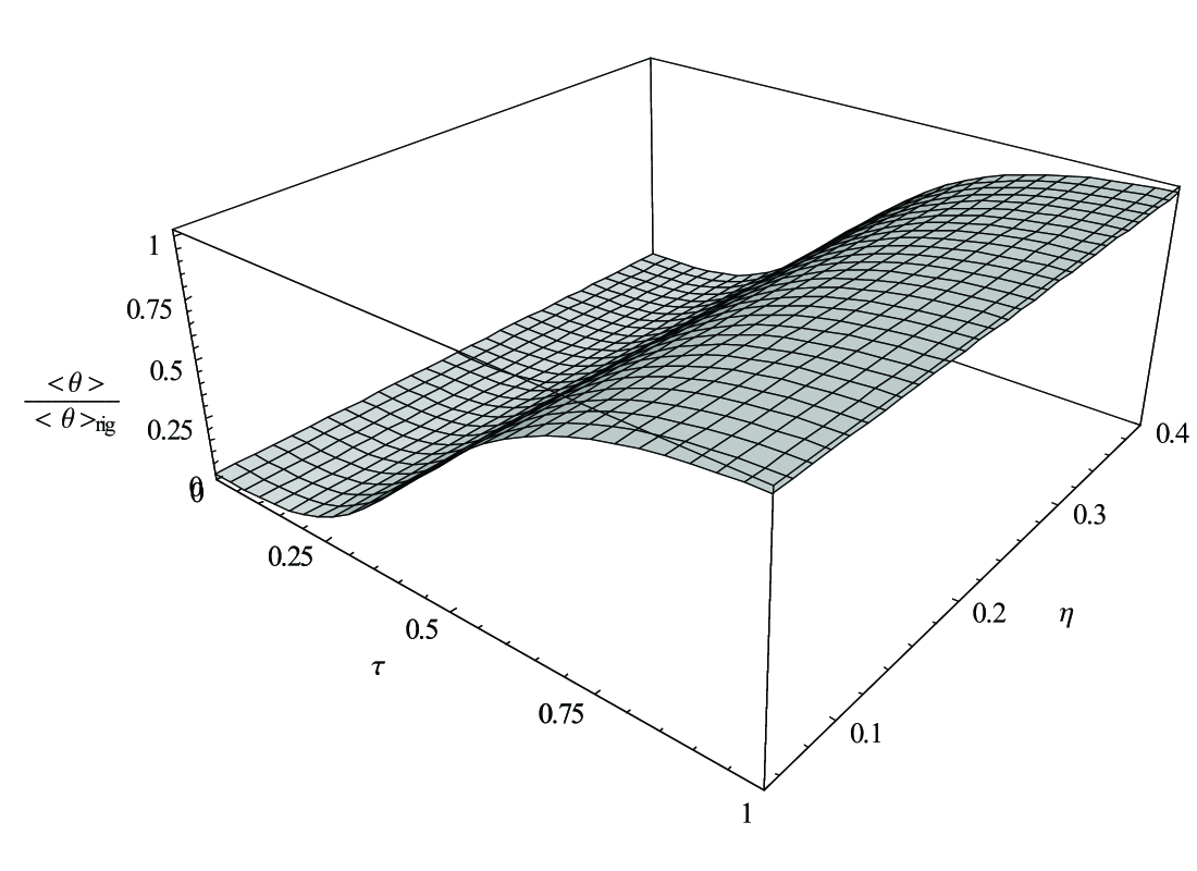
Figure 1: Moment of inertia ${\Theta}$ divided by its rigid value ${\Theta_{rig}}$, as a function of ${\cal T}$ and $\eta$ for $\epsilon_{0}=-0.032$. The trap parameters of Ref. exp3 are used.

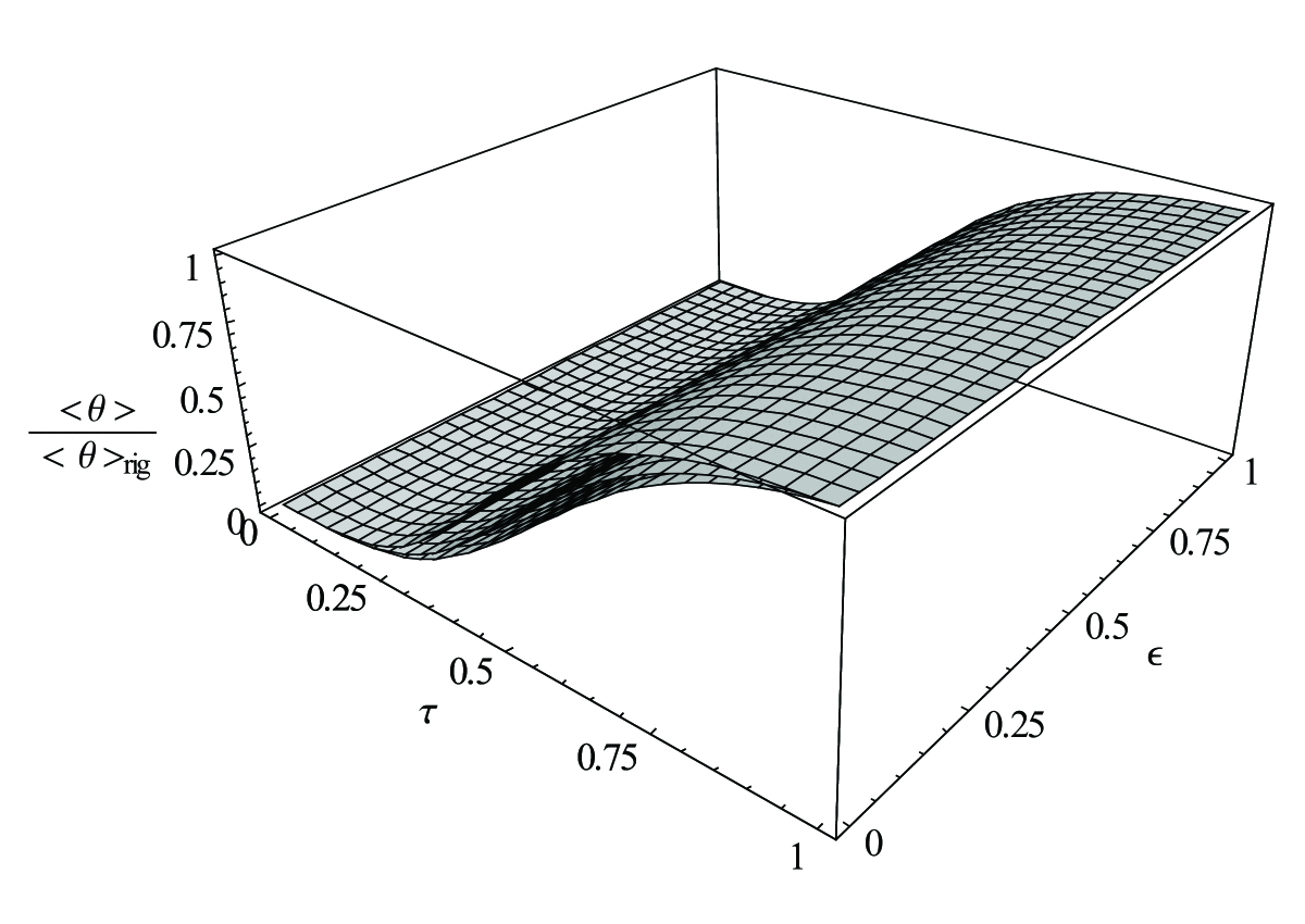
Figure 2: Moment of inertia ${\Theta}$ divided by its rigid value ${\Theta_{rig}}$, as a function of the normalized temperature ${\cal T}$ and the condensate deformation $\epsilon_{0}$ for $\eta$ = 0.2, 0.4. and 0.6 from the bottom to top respectively.

In Fig.(1), $\frac{\Theta}{\Theta_{rig}}$ is represented graphically as a function of ${\cal T}$ and $\eta$ for $\epsilon_{0}=0.031$. The trap parameters of Ref. exp3 are used. This figure shows that $\frac{\Theta}{\Theta_{rig}}$ has a monotonically increasing nature due to the increase of the normalized temperature. This increase is minor in the small temperature range and is rapid in the intermediate temperature range.

Fig.(2) draws $\frac{\Theta}{\Theta_{rig}}$ as a function of $T$ and $\epsilon_{0}$ for different interaction parameter $\eta$. This figure shows that, $\frac{\Theta}{\Theta_{rig}}$ has a monotonically increasing nature due to the increase of the normalized temperature. Moreover, the effect of interaction parameter is clear.

Fig(3) is devoted to illustrate dependence of $\frac{\Theta}{\Theta_{rig}}$ on the interaction parameter $\eta$ and the condensate deformation parameter $\epsilon_{0}$ for different normalized temperature. This figure shows that the dependence of the $\frac{\Theta}{\Theta_{rig}}$ on $\eta$ and $\epsilon_{0}$ is considerably depended on the normalized temperature.

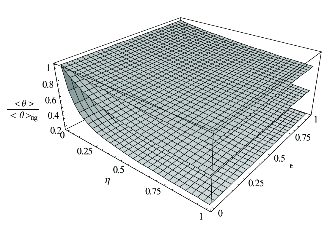
Figure 3: Moment of inertia ${\Theta}$ divided by its rigid value ${\Theta_{rig}}$, as a function of the condensate deformation parameter $\epsilon_{0}$, interaction parameter $\eta$ for normalized temperature $\tau=0.4,0.6$ and 0.8 from the bottom to top respectively.

IV Conclusion

In conclusion, we have shown that the moment of inertia of a gas trapped by a harmonic potential can be explicitly calculated in terms of the in situ radii and temperature dependence for both the condensate and thermal atoms. Interaction affected the value of the moment of inertia by changing its temperature dependence. An interesting feature is noticed that the moment of inertia ${\Theta}$ divided by its rigid value ${\Theta_{rig}}$ has a monotonically rapid increasing nature with the normalized temperature for $0.25<\tau<0.9$. The present analysis recommended Stingari first important conclusion for non-interaction system which is the superfluid effects in the moment of inertia of a harmonically trapped Bose gas should be observable at temperatures not dramatically smaller than the transition temperature for BEC. Our method can be extended to investigate the moment of inertia for system of rotating boson in a combined optical-magnetic trap.

References

(1) M. Matthews, B. Anderson, P. Haljan, D. Hall, C. Wieman,
and E. Cornell, Phys. Rev. Lett 83 (1999) 2498.
(2) K. Madison, F. Chevy, W. Wohlleben, and J. Dalibard,
Phys. Rev. Lett 84 (2000) 806.
(3) J. Abo-Shaeer, C. Raman, J. Vogels, and W. Ketterle,
Science 292 (2001) 476.
(4) K. W. Madison, F. Chevy, V. Bretin, and J. Dalibard,
Phys. Rev. Lett. 86 (2001) 4443.
(5) S. Stringari, Phys. Rev. Lett. 76 (1996) 1405.
(6) F. Brosens, J. T. Devreese, and L. F. Lemmens, Phys.
Rev. A 55 (1997) 2453.
(7) J. Schneider and H. Wallis, Eur. Phys. J. B 18
(2000) 507.
(8) D. Guéry-Odelin and S. Stringari, Phys. Rev. Lett. 83
(1999) 4452.
(9) F. Zambelli and S. Stringarii, Phys. Rev. A 63
(2001) 33602.
(10) A. Recatia, F. Zambellib, and S. Stringarib, Phys. Rev.
Lett. 86 (2001) 377.
(11) J. Annett, Superconductivity, Superfluids and Condensates
(Oxford University Press, 2004).
(12) F. D. S. Giorgini, L. Pitaevskii, and S. Stringari, Rev. of
Mod. Phys. 71 (1999) 463.
(13) S. Sinha, Phys. Rev. A 58 (1998) 3159.
(14) N. Sandoval-Figueroa and V. Romero-Rochin, Phys. Rev.
E 78 (2008) 061129.
(15) Z. X. W. Zhang and L. You, Phys. Rev. A 72
(2005) 053627.
(16) B. H. Bransden and C. J. Joachain, Introduction to Quantum
Mechanics (( Longman, London, 1990).
(17) A. S. Hassan and A. M. El-Badry, Eur. Phys. J. D 68 (2014) 76; A. S. Hassan and S. S. M. Soliman, Phys. Lett. A 380 (2016) 22.
(18) R. Campbell, Thermodynamic properties of a Bose gas with
tuneable interactions (Ph.D. thesis,
Cavendish Laboratory, University of Cambridge, UK,
2011).
(19) V. Bretin, S. Stock, Y. Seurin, and J. Dalibard, Phys. Rev. Lett. 92 (2004) 050403.
(20) H. Haugerud, T. Haugset, and F. Ravndal, Phys. Lett.
A 225 (1997) 18.
(21) N. Tammuz, Thermodynamics of ultracold 39K atomic
Bose gases with tuneable interactions (Ph.D. thesis,
Cavendish Laboratory, University of Cambridge, UK,
2011).
(22) R. K. Pathria, Statistical Mechanics (Pergammon, London,
1972), 1st ed.
(23) S. Giorgini, L. P. Pitaevskii, and S. Stringari, J. Low Temp. Phys. 109 (1997) 309; S. Giorgini, L. Pitaevskii, and S. Stringari, Phys. Rev. Lett. 78 (1997) 3987.
(24) A. L. Fetter, Rev. of Mod. Phys. 81 (2009) 647.
(25) N. R. Cooper, Adv. Phys 57 (2008) 539.
(26) S. Stringari and E. Lipparinri, Phys. Rev. C 22 (1980) 884.
(27) J. R. Abo-Shaeer, C. Raman, and W. Ketterle, Phys. Rev. Lett. 88 (2002) 070409.