Robust High-Dimensional Linear Regression

Abstract

The effectiveness of supervised learning techniques has made them ubiquitous in research and practice. In high-dimensional settings, supervised learning commonly relies on dimensionality reduction to improve performance and identify the most important factors in predicting outcomes. However, the economic importance of learning has made it a natural target for adversarial manipulation of training data, which we term poisoning attacks. Prior approaches to dealing with robust supervised learning rely on strong assumptions about the nature of the feature matrix, such as feature independence and sub-Gaussian noise with low variance. We propose an integrated method for robust regression that relaxes these assumptions, assuming only that the feature matrix can be well approximated by a low-rank matrix. Our techniques integrate improved robust low-rank matrix approximation and robust principle component regression, and yield strong performance guarantees. Moreover, we experimentally show that our methods significantly outperform state of the art both in running time and prediction error.

1 Introduction

Machine learning has come to be widely deployed in a broad array of applications. An important class of applications of machine learning uses it to enable scalable security solutions, such as spam filtering, traffic analysis, and fraud detection [1, 2, 3]. In these applications, reliability of the machine learning system is crucial to ensure service quality and enforce security, but strong incentives exist to reduce learning efficacy (e.g., to bypass spam filters). Indeed, recent research demonstrates that existing systems are vulnerable in the presense of adversaries who can manipulate either the training (i.e. the poisoning attack) or test data (i.e. the evasion attack) [4, 5, 6, 7]. Consequently, an important agenda in machine learning research is to develop learning algorithms that are robust to data manipulation. In this work, we focus on designing supervised learning algorithms that are robust to poisoning attacks.

Existing research on robust machine learning dates back to algorithms for robust PCA [8]. Most of them assume that a portion of the underlying dataset is randomly, rather than adversarially, corrupted. Recently, Chen et al. [9] and Feng et al. [10] considered recovery strategy when the corruption is adversarially chosen to achieve some malicious goal. The former considers a robust linear and the latter logistic regression models. However, both make an extremely strong assumption that each feature is sub-Gaussian with vanishing variance (as $O(\frac{1}{n})$) and features are independent, rendering them impractical and severely limiting the scope of associated theoretical guarantees.

In this work, we propose a novel algorithmic framework for making linear regression robust to data poisoning. Our framework does not require either sub-Gaussian or independence assumptions on the feature matrix X. Instead, we assume that X is generated through adversarial corruption of an approximately low-rank matrix. Our goal is to make regression which uses dimensionality reduction, such as PCA, robust to adversarial manipulation. The technical challenge is two-fold: first, we must make sure that the dimensionality reduction step can reliably recover the low-rank subspace, and second, that the resulting regression performed on the subspace can recover sufficiently accurate predictions, in both cases despite both noise and adversarial examples. While these problems have previously been considered in isolation, ours is the first integrated approach. More significantly, the effectiveness of our approach relies on weaker assumptions than prior art, and, as a result, our proposed practical algorithms significantly outperform state-of-the-art alternatives.

Specifically, we assume that labels y are a linear function of the true feature matrix $\textbf{X}_{\star}$ with additive zero-mean noise. In addition, $\textbf{X}_{\star}$ is corrupted with noise, and the adversary subsequently adds a collection of corrupted rows to the training data. In this model, our approach involves two parts: first, we develop a novel robust matrix factorization algorithm which correctly recovers the subspace whenever this is possible, and second, a trimmed principle component regression, which uses the recovered basis and trimmed optimization to estimate linear model parameters.

Our main contributions are as follows:

• Novel algorithm for robust matrix factorization: We develop a novel algorithm that reliably recovers the low-rank subspace of the feature matrix despite both noise (about which we make few assumptions) and adversarial examples. We prove that our algorithm is effective iff subspace recovery is possible.

• Novel robust regression algorithm with significantly weaker assumptions: In contrast to prior robust regression work, we do not require either feature independence or low-variance sub-Gaussian distribution of features. We prove that our algorithm can reliably learn the low-dimensional linear model despite data corruption and noise.

• Significant improvement in running time and accuracy: We present efficient algorithms which significantly outperform prior art in running time and prediction efficacy.

Related Work: Robust PCA is widely used as a statistical tool for data analysis and dimensionality reduction that is robust to i.i.d. noise [8]. However, these methods cannot deal with “malicious” corruptions, where the sophisticated adversaries can manipulate rows from the subspace of the true feature matrix. In contrast, our approach handles both noise and malicious corruption. Recently, robust learning for several learning models, such as linear and logistic regression have also been proposed [9, 10]. The limitation of these approaches is their assumption that the feature matrix is sub-Gaussian with vanishing variance, and that features are independent. Our approach, in contrast, only assumes that the true feature matrix (prior to corruption) is low rank. Yan et al. proposed an outlier pursuit algorithm to deal with the matrix completion problem with corruptions [11], and a similar algorithm is applied by Xu et al. to deal with the noisy version of feature matrix [12]. However, these methods only consider the matrix recovery problem and are not scalable. A more scalable algorithm based on the alternating minimization approach was recently proposed by Rodriguez et al. [13]; however, this method does not consider data noise or corruption. A number of heuristic techniques have also been proposed for poisoning attacks [14, 15, 16] for other problems, such as robust anomaly detection source identification.

2 Problem Setup and Solution Overview

We start with the pristine training dataset of $n$ labeled examples, $\langle\textbf{X}_{\star},\textbf{y}_{\star}\rangle$, which subsequently suffers from two types of corruption: noise is added to feature vectors, and the adversary adds $n_{1}$ malicious examples (feature vectors and labels) to best mislead the learning. We assume that the adversary has full knowledge of the learning algorithm. The learner’s goal is to learn a model on the corrupted dataset which is similar to the true model. The feature space is high-dimensional, and the learner will perform dimensionality reduction prior to learning. In particular, we assume that $\textbf{X}_{\star}$ is low-rank with a basis B, and we assume that the true model is the associated low-dimensional linear regression.

Formally, observed training data is generated as follows:

1. Ground truth: $\textbf{y}_{\star}=\textbf{X}_{\star}\beta^{\star}=\textbf{U}\beta^{\star}_{U}$, where $\beta^{\star}$ is the true model, $\beta^{\star}_{U}$ is its low-dimensional representation, and $\textbf{U}=\textbf{X}_{\star}B$ is the low-dimensional embedding of $\textbf{X}_{\star}$.

2. Noise: $\textbf{X}_{0}=\textbf{X}_{\star}+\textbf{N}$, where N is a noise matrix with $\|\textbf{N}\|_{\infty}\leq\epsilon$; $\textbf{y}_{0}=\textbf{y}_{\star}+e$, where $e$ is i.i.d. zero-mean Gaussian noise with variance $\sigma$.

3. Corruption: The attacker adds $n_{1}$ adversarially crafted examples $(\textbf{x}_{a},\textbf{y}_{a})$ to get $\langle\textbf{X},\textbf{y}\rangle$, which maximally skews prediction performance of low-dimensional linear regression.

To formally characterize how well the learner performs in this setting, we define (1) a model function $f(\textbf{X}_{0},\textbf{y}_{0})$ which is the model learned on $\langle\textbf{X}_{\star},\textbf{y}_{\star}\rangle$; (2) a loss function $l$; and (3) a threshold function $\delta(z)$ which takes as input $z>1$, and is increasing in $z$. Our metric is $(f,l,\delta)$-tolerance:

Definition 1 ($(f,l,\delta)$-tolerance).

We say that learner $\mathcal{L}$ is $(f,l,\delta)$-tolerant, if for any attacker, and any $z>1$, we have $l(\mathcal{L}(\textbf{X},\textbf{y}),f(\textbf{X}_{0},\textbf{y}_{0}))\leq\delta(z)$ with probability at least $1-c_{1}z^{-c_{2}}$, for some constant $c_{1},c_{2}>0$.

In our setting, $f(\textbf{X}_{0},\textbf{y}_{0})$ return $\beta^{\star}$ and $l$ is expected quadratic loss $E_{x}\big{[}(x(\leavevmode\hbox{\set@color\hskip 36.2pt\leavevmode\hbox{\set@color$\beta$}\raisebox{9.858pt}{$\leavevmode\hbox{\set@color\raisebox{-0.95679pt}{\leavevmode\resizebox{72.4pt}{1.19598pt}{\leavevmode\hbox{\set@color$\mathchoice{\raisebox{-112.41994pt}{\leavevmode\resizebox{22.62498pt}{393.47006pt}{\leavevmode\hbox{\set@color$\displaystyle\mathchoice{\raisebox{0.0pt}{\leavevmode\resizebox{5.65625pt}{393.47pt}{\leavevmode\hbox{\set@color$\displaystyle\kern-0.6pt\bigwedge\kern-0.6pt$}}}}{\raisebox{0.0pt}{\leavevmode\resizebox{5.65625pt}{393.47pt}{\leavevmode\hbox{\set@color$\textstyle\kern-0.6pt\bigwedge\kern-0.6pt$}}}}{\raisebox{0.0pt}{\leavevmode\resizebox{5.65625pt}{393.47028pt}{\leavevmode\hbox{\set@color$\scriptstyle\kern-0.6pt\bigwedge\kern-0.6pt$}}}}{\raisebox{0.0pt}{\leavevmode\resizebox{5.65625pt}{393.47pt}{\leavevmode\hbox{\set@color$\scriptscriptstyle\kern-0.6pt\bigwedge\kern-0.6pt$}}}}$}}}}{\raisebox{-112.41994pt}{\leavevmode\resizebox{22.62498pt}{393.47006pt}{\leavevmode\hbox{\set@color$\textstyle\mathchoice{\raisebox{0.0pt}{\leavevmode\resizebox{5.65625pt}{393.47pt}{\leavevmode\hbox{\set@color$\displaystyle\kern-0.6pt\bigwedge\kern-0.6pt$}}}}{\raisebox{0.0pt}{\leavevmode\resizebox{5.65625pt}{393.47pt}{\leavevmode\hbox{\set@color$\textstyle\kern-0.6pt\bigwedge\kern-0.6pt$}}}}{\raisebox{0.0pt}{\leavevmode\resizebox{5.65625pt}{393.47028pt}{\leavevmode\hbox{\set@color$\scriptstyle\kern-0.6pt\bigwedge\kern-0.6pt$}}}}{\raisebox{0.0pt}{\leavevmode\resizebox{5.65625pt}{393.47pt}{\leavevmode\hbox{\set@color$\scriptscriptstyle\kern-0.6pt\bigwedge\kern-0.6pt$}}}}$}}}}{\raisebox{-112.41978pt}{\leavevmode\resizebox{15.83752pt}{393.47021pt}{\leavevmode\hbox{\set@color$\scriptstyle\mathchoice{\raisebox{0.0pt}{\leavevmode\resizebox{3.95938pt}{393.47028pt}{\leavevmode\hbox{\set@color$\displaystyle\kern-0.6pt\bigwedge\kern-0.6pt$}}}}{\raisebox{0.0pt}{\leavevmode\resizebox{3.95938pt}{393.47028pt}{\leavevmode\hbox{\set@color$\textstyle\kern-0.6pt\bigwedge\kern-0.6pt$}}}}{\raisebox{0.0pt}{\leavevmode\resizebox{3.95938pt}{393.4702pt}{\leavevmode\hbox{\set@color$\scriptstyle\kern-0.6pt\bigwedge\kern-0.6pt$}}}}{\raisebox{0.0pt}{\leavevmode\resizebox{3.95938pt}{393.47028pt}{\leavevmode\hbox{\set@color$\scriptscriptstyle\kern-0.6pt\bigwedge\kern-0.6pt$}}}}$}}}}{\raisebox{-112.41994pt}{\leavevmode\resizebox{11.3125pt}{393.47006pt}{\leavevmode\hbox{\set@color$\scriptscriptstyle\mathchoice{\raisebox{0.0pt}{\leavevmode\resizebox{2.82813pt}{393.47pt}{\leavevmode\hbox{\set@color$\displaystyle\kern-0.6pt\bigwedge\kern-0.6pt$}}}}{\raisebox{0.0pt}{\leavevmode\resizebox{2.82813pt}{393.47pt}{\leavevmode\hbox{\set@color$\textstyle\kern-0.6pt\bigwedge\kern-0.6pt$}}}}{\raisebox{0.0pt}{\leavevmode\resizebox{2.82813pt}{393.47028pt}{\leavevmode\hbox{\set@color$\scriptstyle\kern-0.6pt\bigwedge\kern-0.6pt$}}}}{\raisebox{0.0pt}{\leavevmode\resizebox{2.82813pt}{393.47pt}{\leavevmode\hbox{\set@color$\scriptscriptstyle\kern-0.6pt\bigwedge\kern-0.6pt$}}}}$}}}}$}}}}$}\hskip 36.2pt}-\beta^{\star}))^{2}\big{]}$.

For convenience, we let $\mathcal{O}$ denote the set of (unknown) indices of the samples in X coming from $\textbf{X}_{0}$ and $\mathcal{A}=\{1,...,n+n_{1}\}-\mathcal{O}$ the set of indices for adversarial samples in X. For an index set $\mathcal{I}$ and matrix $M$, $M^{\mathcal{I}}$ denotes the sub-matrix containing only rows in $\mathcal{I}$; similar notation is used for vectors. We define $\gamma=\frac{n_{1}}{n}$ as the corruption ratio, or the ratio of corrupted and pristine data.

2.1 Solution overview and paper organization

Our goal is to design a learner $\mathcal{L}$ to estimate the coefficients            $\beta$ $\textstyle\kern-0.6pt\bigwedge\kern-0.6pt$             of the true model $\beta^{\star}$ using low-dimensional embedding of a high-dimensional model. We achieve this goal in two steps: (1) recover the subspace B of $\textbf{X}_{\star}$; (2) project X onto B, and estimate            $\beta$ $\textstyle\kern-0.6pt\bigwedge\kern-0.6pt$             using robust principle component regression. The key challenge is that an adversary can design corrupted data to interfere both with the first and second step of the process.

For the first step (Section 3), we develop a robust subspace recovery algorithm which can account for both noise N and adversarial examples in correctly recovering the subspace of $\textbf{X}_{\star}$. We characterize necessary and sufficient conditions for successful subspace recovery, showing that our algorithm succeeds whenever recovery is possible. The challenge in the second step (Section 4) is that the adversary can construct $\textbf{X}^{\mathcal{A}}$ from the same subspace as $\textbf{X}_{\star}$, but with the different distribution of $\langle\textbf{X}^{\mathcal{A}},\textbf{y}^{\mathcal{A}}\rangle$ from $\langle\textbf{X}_{\star},\textbf{y}_{\star}\rangle$. To address this, we propose the trimmed principle component regression algorithm to minimize the loss function over only a subset of the dataset ensuring that the adversary can have only a limited impact by adding $n_{1}$ arbitrary corrupted samples without having these instances being discarded. Our theoretical results demonstrate that the combined approach is $(f,l,\delta)$-tolerant learning algorithm. Finally, in Section 5, we present an efficient practical implementation of our methods, which we evaluate in Section 6.

In our analysis, we use the corruption parameter $n_{1}$ and the rank $k$ of the low-dimensional embedding to characterize the theoretical results. In our experiments, however, we show that we only require a lower bound on $n_{1}$ and an upper bound on $k$ for our techniques to work.

3 Robust Subspace Recovery

In this section, we discuss how to recover the low-rank subspace of $\textbf{X}_{\star}$ from X. Our goal is to exactly recover the low-rank subspace, i.e., returning a basis for $\textbf{X}_{\star}$. We show sufficient and necessary conditions for this problem to be solvable, and provide algorithms when this is possible. As a warmup, we first discuss the noise-free version of the problem, and then present our results for the problem with noises. Proofs of the theorems presented in this section can be found in Appendix A. Formally, we consider the following problem:

Problem Definition 1 (Subspace Recovery).

Design an algorithm $\mathcal{L}_{\text{recovery}}$, which takes as input X, and returns a set of vectors $B$ which form the basis of $\textbf{X}_{\star}$.

3.1 Warmup: Noise-free Subspace Recovery

We first consider an easier version of Problem 1 with $N=0$. In this case, we know that $\textbf{X}^{\mathcal{O}}=\textbf{X}_{\star}$. We assume that we know ${\mathrm{rank}(\textbf{X}_{\star})}=k$ (or have an upper bound on it). Below we demonstrate that there exists a sharp threshold $\theta$ on $n_{1}$ such that whenever $n_{1}<\theta$, we can solve Problem 1 exactly with high probability, whereas if $n_{1}\geq\theta$, Problem 1 cannot be solved. To characterize this threshold, we define the cardinality of the maximal rank $k-1$ subspace $\mathit{MS}_{k-1}(\textbf{X}_{\star})$ as the optimal value of the following problem:

$$\max_{\mathcal{I}}|\mathcal{I}|~{}~{}\text{s.t.}~{}~{}{\mathrm{rank}(\textbf{X}_{\star}^{\mathcal{I}})}\leq k-1$$

Intuitively, the adversary can insert $n_{1}=n-\mathit{MS}_{k-1}(\textbf{X}_{\star})$ samples to form a rank $k$ subspace, which does not span $\textbf{X}_{\star}$. The following theorem shows that in this case, there is indeed no learner that can successfully recover the subspace of $\textbf{X}_{\star}$.

Theorem 1.

If $n_{1}+\mathit{MS}_{k-1}(\textbf{X}_{\star})\geq n$, then there exists an adversary such that no algorithm $\mathcal{L}_{\text{recover}}$ solves Problem 1 with probability greater than $1/2$.

On the other hand, when $n_{1}$ is below this threshold, we can use the following simple algorithm to recover the subspace of $\textbf{X}_{\star}$:

Algorithm 1 Exact recover algorithm for Problem 1 (Noisy-free)

We search for a subset $\mathcal{I}$ of indices, such that $|\mathcal{I}|=n$, and ${\mathrm{rank}(\textbf{X}^{\mathcal{I}})}=k$
return a basis of $\textbf{X}^{\mathcal{I}}$.

In fact, we can prove the following theorem.

Theorem 2.

If $n_{1}+\mathit{MS}_{k-1}(\textbf{X}_{\star})<n$, then Algorithm  1 solves Problem 1 for any adversary.

Theorems 1 and 2 together give the necessary and sufficient conditions on when Problem 1 is solvable, and Algorithm 1 provides a solution. We further show an implication of these theorems on the corruption ratio $\gamma$. We can prove that $\mathit{MS}_{k-1}(\textbf{X}_{\star})\geq k-1$ (see Appendix A). Combining this with Theorem 1, we can have the following upper bound on $\gamma$.

Corollary 1.

If $\gamma\geq 1-\frac{k-1}{n}$, then Problem 1 cannot be solved.

3.2 Dealing with Noise

We now consider Problem 1 with noise. Before we discuss the adversary, we first need to assume that the uncorrupted version is solvable. In particular, we assume that $X_{\star}$ optimizes the following problem:

$$\min_{\textbf{X}^{\prime}}||\textbf{X}_{0}-\textbf{X}^{\prime}||$$ (1a)

$$\text{s.t.}~{}~{}{\mathrm{rank}(\textbf{X}^{\prime})}\leq k.$$ (1b)

Without otherwise mentioned, we use $||\cdot||$ to denote the Frobenius norm. We put no additional restrictions on N except above. Note that this assumption is implied by the classical PCA problem [17, 18, 19]. We want to emphasize on the optimal value of the above problem. We denote this value to be noise residual, denoted as $\mathit{NR}(\textbf{X}_{0})=\textbf{N}$. Noise residual is a key component to characterize the necessary and sufficient condition for the solvability of Problem  1.

Characterization of the defender’s ability to accurately recover the true basis B of $\textbf{X}_{\star}$ after the attacker adds $n_{1}$ malicious instances stems from the attacker’s ability to mislead the defender into thinking that some other basis, $\bar{\textbf{B}}$, better represents $\textbf{X}_{\star}$. Intuitively, since the defender does not know $\textbf{X}_{0}$, $\textbf{X}_{\star}$, or which $n_{1}$ rows of the data matrix X are adversarial, this comes down to the ability to identify the $n-n_{1}$ rows that correspond to the correct basis (note that it will suffice to obtain the correct basis even if some adversarial rows are used, since the adversary may be forced to align malicious examples with the correct basis to evade explicit detection). As we show below, whether the defender can succeed is determined by the relationship between the noise residual $\mathit{NR}(\textbf{X}_{0})$ and sub-matrix residual, denoted as $\mathit{SR}(\textbf{X}_{0})$, which we define as the value optimizing the following problem:

$$\min_{\mathcal{I},\textbf{B},\textbf{U}}||\textbf{X}_{0}^{\mathcal{I}}-\textbf{U}\bar{\textbf{B}}||$$ (2a)

s.t. $$\quad{\mathrm{rank}(\bar{\textbf{B}})}=k,\bar{\textbf{B}}\bar{\textbf{B}}^{T}=I_{k},\textbf{X}_{\star}\bar{\textbf{B}}^{T}\bar{\textbf{B}}\neq\textbf{X}_{\star}$$ (2b)

$$\mathcal{I}\subseteq\{1,2,...,n\},|\mathcal{I}|=n-n_{1}.$$ (2c)

We now explain the above optimization problem. $U$ and $\bar{\textbf{B}}$ are $n\times k$ and $k\times m$ matrixes separately. Here $\bar{\textbf{B}}$ is a basis which the attacker “targets”; for convenience, we require $\bar{\textbf{B}}$ to be orthogonal (i.e., $\bar{\textbf{B}}\bar{\textbf{B}}^{T}=I_{k}$). Since the attacker succeeds only if they can induce a basis different from the true B, we require that $\bar{\textbf{B}}$ does not span of $\textbf{X}_{\star}$, which is equivalent to saying $\textbf{X}_{\star}\bar{\textbf{B}}^{T}\bar{\textbf{B}}\neq\textbf{X}_{\star}$. Thus, this optimization problem seeks $n-n_{1}$ rows of $\textbf{X}_{\star}$, where $\mathcal{I}$ is the corresponding index set. The objective is to minimize the distance between $\textbf{X}_{0}^{\mathcal{I}}$ and the span space of the target basis $\bar{\textbf{B}}$, (i.e., $||\textbf{X}_{0}^{\mathcal{I}}-\textbf{U}\bar{\textbf{B}}||$).

Algorithm 2 Exact recovery algorithm for Problem 1

Solve the following optimization problem and get $\mathcal{I}$.

$${\begin{array}[]{c}\min_{\mathcal{I},L}||\textbf{X}^{\mathcal{I}}-L||\\ \text{s.t.}~{}~{}{\mathrm{rank}(L)}\leq k,I\subseteq\{1,...,n+n_{1}\},|I|=n\end{array}}$$ (3)

return a basis of $\textbf{X}^{\mathcal{I}}$.

To understand the importance of $\mathit{SR}(\textbf{X}_{0})$, consider Algorithm 2 for recovering the basis of $\textbf{X}_{\star}$, B. If the optimal objective value of optimization problem (2), $\mathit{SR}(\textbf{X}_{0})$, exceeds the noise $\mathit{NR}(\textbf{X}_{0})$, it follows that the defender can obtain the correct basis B using Algorithm 2, as it yields a better low-rank approximation of X than any other basis. Else, it is, indeed, possible for the adversary to induce an incorrect choice of basis. The following theorem formalizes this argument.

Theorem 3.

If $\mathit{SR}(\textbf{X}_{0})\leq\mathit{NR}(\textbf{X}_{0})$, then no algorithm recovers the exact subspace of $\textbf{X}_{\star}$ with probability greater than $1/2$. If $\mathit{SR}(\textbf{X}_{0})>\mathit{NR}(\textbf{X}_{0})$, then Algorithm 2 solves Problem 1.

To draw connection between the noisy case and the noise-free case, we can view Theorem 1 and 2 as special cases of Theorem  3.

Theorem 4.

When $\textbf{N}=0$, $\mathit{SR}(\textbf{X}_{0})>\mathit{NR}(\textbf{X}_{0})=0$ if and only if $n_{1}+\mathit{MS}_{k-1}(\textbf{X}_{\star})<n$.

4 Trimmed Principal Component Regression

In this section, we present trimmed principal component regression (T-PCR) algorithm. The key idea is to leverage the principal component regression (PCR) approach to estimate            $\beta$ $\textstyle\kern-0.6pt\bigwedge\kern-0.6pt$            , but during the process trimming out those malicious samples that try to deviate the estimator from the true ones. In the following, we present the approach, which is similar to the standard PCR approach, though we do not require computing the exact singular vectors of $\textbf{X}_{\star}$.

Assume we recover a basis B of $\textbf{X}_{\star}$. Without loss of generality, we assume that B is an orthogonal basis of $k$ row vectors. Since B is a basis for $\textbf{X}_{\star}$, we assume $\textbf{X}_{\star}=\textbf{U}_{\star}\textbf{B}$. Then we know that, by optimization (1), $\textbf{U}_{\star}=\text{argmin}_{U}||\textbf{X}_{0}-U\textbf{B}||$. We compute $\textbf{U}=\text{argmin}_{U}||\textbf{X}-U\textbf{B}||$, and, by definition, we know $\textbf{U}_{\star}=\textbf{U}^{\mathcal{O}}$. By OLS estimator, we know that $\textbf{U}^{T}=(\textbf{B}\textbf{B}^{T})^{-1}\textbf{B}\textbf{X}^{T}$, and thus $\textbf{U}=\textbf{X}\textbf{B}^{T}$.

To estimate $\textbf{y}=\textbf{X}_{\star}\beta+e$, we assume $\beta_{U}=\textbf{B}\beta$. Since $\textbf{X}_{\star}=\textbf{U}_{\star}\textbf{B}$, we convert the estimation problem of $\beta$ from a high dimensional space to the estimation problem of $\beta_{U}$ from a low dimensional space, such that $y=\textbf{U}\beta_{U}+e$. After estimating for                     $\beta_{U}$ $\textstyle\kern-0.6pt\bigwedge\kern-0.6pt$                     , we can convert it back to get $\leavevmode\hbox{\set@color\hskip 36.2pt\leavevmode\hbox{\set@color$\beta$}\raisebox{9.858pt}{$\leavevmode\hbox{\set@color\raisebox{-0.95679pt}{\leavevmode\resizebox{72.4pt}{1.19598pt}{\leavevmode\hbox{\set@color$\mathchoice{\raisebox{-112.41994pt}{\leavevmode\resizebox{22.62498pt}{393.47006pt}{\leavevmode\hbox{\set@color$\displaystyle\mathchoice{\raisebox{0.0pt}{\leavevmode\resizebox{5.65625pt}{393.47pt}{\leavevmode\hbox{\set@color$\displaystyle\kern-0.6pt\bigwedge\kern-0.6pt$}}}}{\raisebox{0.0pt}{\leavevmode\resizebox{5.65625pt}{393.47pt}{\leavevmode\hbox{\set@color$\textstyle\kern-0.6pt\bigwedge\kern-0.6pt$}}}}{\raisebox{0.0pt}{\leavevmode\resizebox{5.65625pt}{393.47028pt}{\leavevmode\hbox{\set@color$\scriptstyle\kern-0.6pt\bigwedge\kern-0.6pt$}}}}{\raisebox{0.0pt}{\leavevmode\resizebox{5.65625pt}{393.47pt}{\leavevmode\hbox{\set@color$\scriptscriptstyle\kern-0.6pt\bigwedge\kern-0.6pt$}}}}$}}}}{\raisebox{-112.41994pt}{\leavevmode\resizebox{22.62498pt}{393.47006pt}{\leavevmode\hbox{\set@color$\textstyle\mathchoice{\raisebox{0.0pt}{\leavevmode\resizebox{5.65625pt}{393.47pt}{\leavevmode\hbox{\set@color$\displaystyle\kern-0.6pt\bigwedge\kern-0.6pt$}}}}{\raisebox{0.0pt}{\leavevmode\resizebox{5.65625pt}{393.47pt}{\leavevmode\hbox{\set@color$\textstyle\kern-0.6pt\bigwedge\kern-0.6pt$}}}}{\raisebox{0.0pt}{\leavevmode\resizebox{5.65625pt}{393.47028pt}{\leavevmode\hbox{\set@color$\scriptstyle\kern-0.6pt\bigwedge\kern-0.6pt$}}}}{\raisebox{0.0pt}{\leavevmode\resizebox{5.65625pt}{393.47pt}{\leavevmode\hbox{\set@color$\scriptscriptstyle\kern-0.6pt\bigwedge\kern-0.6pt$}}}}$}}}}{\raisebox{-112.41978pt}{\leavevmode\resizebox{15.83752pt}{393.47021pt}{\leavevmode\hbox{\set@color$\scriptstyle\mathchoice{\raisebox{0.0pt}{\leavevmode\resizebox{3.95938pt}{393.47028pt}{\leavevmode\hbox{\set@color$\displaystyle\kern-0.6pt\bigwedge\kern-0.6pt$}}}}{\raisebox{0.0pt}{\leavevmode\resizebox{3.95938pt}{393.47028pt}{\leavevmode\hbox{\set@color$\textstyle\kern-0.6pt\bigwedge\kern-0.6pt$}}}}{\raisebox{0.0pt}{\leavevmode\resizebox{3.95938pt}{393.4702pt}{\leavevmode\hbox{\set@color$\scriptstyle\kern-0.6pt\bigwedge\kern-0.6pt$}}}}{\raisebox{0.0pt}{\leavevmode\resizebox{3.95938pt}{393.47028pt}{\leavevmode\hbox{\set@color$\scriptscriptstyle\kern-0.6pt\bigwedge\kern-0.6pt$}}}}$}}}}{\raisebox{-112.41994pt}{\leavevmode\resizebox{11.3125pt}{393.47006pt}{\leavevmode\hbox{\set@color$\scriptscriptstyle\mathchoice{\raisebox{0.0pt}{\leavevmode\resizebox{2.82813pt}{393.47pt}{\leavevmode\hbox{\set@color$\displaystyle\kern-0.6pt\bigwedge\kern-0.6pt$}}}}{\raisebox{0.0pt}{\leavevmode\resizebox{2.82813pt}{393.47pt}{\leavevmode\hbox{\set@color$\textstyle\kern-0.6pt\bigwedge\kern-0.6pt$}}}}{\raisebox{0.0pt}{\leavevmode\resizebox{2.82813pt}{393.47028pt}{\leavevmode\hbox{\set@color$\scriptstyle\kern-0.6pt\bigwedge\kern-0.6pt$}}}}{\raisebox{0.0pt}{\leavevmode\resizebox{2.82813pt}{393.47pt}{\leavevmode\hbox{\set@color$\scriptscriptstyle\kern-0.6pt\bigwedge\kern-0.6pt$}}}}$}}}}$}}}}$}\hskip 36.2pt}=\textbf{B}\leavevmode\hbox{\set@color\hskip 66.6052pt\leavevmode\hbox{\set@color$\beta_{U}$}\raisebox{9.858pt}{$\leavevmode\hbox{\set@color\raisebox{-0.95679pt}{\leavevmode\resizebox{133.2104pt}{1.19598pt}{\leavevmode\hbox{\set@color$\mathchoice{\raisebox{-112.41994pt}{\leavevmode\resizebox{40.36137pt}{393.47006pt}{\leavevmode\hbox{\set@color$\displaystyle\mathchoice{\raisebox{0.0pt}{\leavevmode\resizebox{10.09035pt}{393.47pt}{\leavevmode\hbox{\set@color$\displaystyle\kern-0.6pt\bigwedge\kern-0.6pt$}}}}{\raisebox{0.0pt}{\leavevmode\resizebox{10.09035pt}{393.47pt}{\leavevmode\hbox{\set@color$\textstyle\kern-0.6pt\bigwedge\kern-0.6pt$}}}}{\raisebox{0.0pt}{\leavevmode\resizebox{10.09035pt}{393.47028pt}{\leavevmode\hbox{\set@color$\scriptstyle\kern-0.6pt\bigwedge\kern-0.6pt$}}}}{\raisebox{0.0pt}{\leavevmode\resizebox{10.09035pt}{393.47pt}{\leavevmode\hbox{\set@color$\scriptscriptstyle\kern-0.6pt\bigwedge\kern-0.6pt$}}}}$}}}}{\raisebox{-112.41994pt}{\leavevmode\resizebox{40.36137pt}{393.47006pt}{\leavevmode\hbox{\set@color$\textstyle\mathchoice{\raisebox{0.0pt}{\leavevmode\resizebox{10.09035pt}{393.47pt}{\leavevmode\hbox{\set@color$\displaystyle\kern-0.6pt\bigwedge\kern-0.6pt$}}}}{\raisebox{0.0pt}{\leavevmode\resizebox{10.09035pt}{393.47pt}{\leavevmode\hbox{\set@color$\textstyle\kern-0.6pt\bigwedge\kern-0.6pt$}}}}{\raisebox{0.0pt}{\leavevmode\resizebox{10.09035pt}{393.47028pt}{\leavevmode\hbox{\set@color$\scriptstyle\kern-0.6pt\bigwedge\kern-0.6pt$}}}}{\raisebox{0.0pt}{\leavevmode\resizebox{10.09035pt}{393.47pt}{\leavevmode\hbox{\set@color$\scriptscriptstyle\kern-0.6pt\bigwedge\kern-0.6pt$}}}}$}}}}{\raisebox{-112.41978pt}{\leavevmode\resizebox{28.50635pt}{393.47021pt}{\leavevmode\hbox{\set@color$\scriptstyle\mathchoice{\raisebox{0.0pt}{\leavevmode\resizebox{7.12659pt}{393.47028pt}{\leavevmode\hbox{\set@color$\displaystyle\kern-0.6pt\bigwedge\kern-0.6pt$}}}}{\raisebox{0.0pt}{\leavevmode\resizebox{7.12659pt}{393.47028pt}{\leavevmode\hbox{\set@color$\textstyle\kern-0.6pt\bigwedge\kern-0.6pt$}}}}{\raisebox{0.0pt}{\leavevmode\resizebox{7.12659pt}{393.4702pt}{\leavevmode\hbox{\set@color$\scriptstyle\kern-0.6pt\bigwedge\kern-0.6pt$}}}}{\raisebox{0.0pt}{\leavevmode\resizebox{7.12659pt}{393.47028pt}{\leavevmode\hbox{\set@color$\scriptscriptstyle\kern-0.6pt\bigwedge\kern-0.6pt$}}}}$}}}}{\raisebox{-112.41994pt}{\leavevmode\resizebox{23.98131pt}{393.47006pt}{\leavevmode\hbox{\set@color$\scriptscriptstyle\mathchoice{\raisebox{0.0pt}{\leavevmode\resizebox{5.99533pt}{393.47pt}{\leavevmode\hbox{\set@color$\displaystyle\kern-0.6pt\bigwedge\kern-0.6pt$}}}}{\raisebox{0.0pt}{\leavevmode\resizebox{5.99533pt}{393.47pt}{\leavevmode\hbox{\set@color$\textstyle\kern-0.6pt\bigwedge\kern-0.6pt$}}}}{\raisebox{0.0pt}{\leavevmode\resizebox{5.99533pt}{393.47028pt}{\leavevmode\hbox{\set@color$\scriptstyle\kern-0.6pt\bigwedge\kern-0.6pt$}}}}{\raisebox{0.0pt}{\leavevmode\resizebox{5.99533pt}{393.47pt}{\leavevmode\hbox{\set@color$\scriptscriptstyle\kern-0.6pt\bigwedge\kern-0.6pt$}}}}$}}}}$}}}}$}\hskip 66.6052pt}$. Notice that this is similar to principal component regression [20].

However, the adversary may corrupt $n_{1}$ rows in U to fool the learner to make a wrong estimation on                     $\beta_{U}$ $\textstyle\kern-0.6pt\bigwedge\kern-0.6pt$                     , and thus on            $\beta$ $\textstyle\kern-0.6pt\bigwedge\kern-0.6pt$            . To mitigate this problem, we design Algorithm 3.

Algorithm 3 Trimmed Principal Component Regression

Input: $\textbf{X},\textbf{y}$

1. Use Algorithm 2 to compute a basis from X, and orthogonalize it to get B

2. Project X onto the span space of B and get $\textbf{U}\leftarrow\textbf{X}\textbf{B}^{T}$

3. Solve the following minimization problem to get                     $\beta_{U}$ $\textstyle\kern-0.6pt\bigwedge\kern-0.6pt$                     

   $$\min_{\beta_{U}}\sum_{j=1}^{n}\{(y_{i}-u_{i}\beta_{U})^{2}\text{ for }i=1,...,n+n_{1}\}_{(j)}$$ (4)

   where $z_{(j)}$ denotes the $j$-th smallest element in sequence $z$.

4. return $\leavevmode\hbox{\set@color\hskip 36.2pt\leavevmode\hbox{\set@color$\beta$}\raisebox{9.858pt}{$\leavevmode\hbox{\set@color\raisebox{-0.95679pt}{\leavevmode\resizebox{72.4pt}{1.19598pt}{\leavevmode\hbox{\set@color$\mathchoice{\raisebox{-112.41994pt}{\leavevmode\resizebox{22.62498pt}{393.47006pt}{\leavevmode\hbox{\set@color$\displaystyle\mathchoice{\raisebox{0.0pt}{\leavevmode\resizebox{5.65625pt}{393.47pt}{\leavevmode\hbox{\set@color$\displaystyle\kern-0.6pt\bigwedge\kern-0.6pt$}}}}{\raisebox{0.0pt}{\leavevmode\resizebox{5.65625pt}{393.47pt}{\leavevmode\hbox{\set@color$\textstyle\kern-0.6pt\bigwedge\kern-0.6pt$}}}}{\raisebox{0.0pt}{\leavevmode\resizebox{5.65625pt}{393.47028pt}{\leavevmode\hbox{\set@color$\scriptstyle\kern-0.6pt\bigwedge\kern-0.6pt$}}}}{\raisebox{0.0pt}{\leavevmode\resizebox{5.65625pt}{393.47pt}{\leavevmode\hbox{\set@color$\scriptscriptstyle\kern-0.6pt\bigwedge\kern-0.6pt$}}}}$}}}}{\raisebox{-112.41994pt}{\leavevmode\resizebox{22.62498pt}{393.47006pt}{\leavevmode\hbox{\set@color$\textstyle\mathchoice{\raisebox{0.0pt}{\leavevmode\resizebox{5.65625pt}{393.47pt}{\leavevmode\hbox{\set@color$\displaystyle\kern-0.6pt\bigwedge\kern-0.6pt$}}}}{\raisebox{0.0pt}{\leavevmode\resizebox{5.65625pt}{393.47pt}{\leavevmode\hbox{\set@color$\textstyle\kern-0.6pt\bigwedge\kern-0.6pt$}}}}{\raisebox{0.0pt}{\leavevmode\resizebox{5.65625pt}{393.47028pt}{\leavevmode\hbox{\set@color$\scriptstyle\kern-0.6pt\bigwedge\kern-0.6pt$}}}}{\raisebox{0.0pt}{\leavevmode\resizebox{5.65625pt}{393.47pt}{\leavevmode\hbox{\set@color$\scriptscriptstyle\kern-0.6pt\bigwedge\kern-0.6pt$}}}}$}}}}{\raisebox{-112.41978pt}{\leavevmode\resizebox{15.83752pt}{393.47021pt}{\leavevmode\hbox{\set@color$\scriptstyle\mathchoice{\raisebox{0.0pt}{\leavevmode\resizebox{3.95938pt}{393.47028pt}{\leavevmode\hbox{\set@color$\displaystyle\kern-0.6pt\bigwedge\kern-0.6pt$}}}}{\raisebox{0.0pt}{\leavevmode\resizebox{3.95938pt}{393.47028pt}{\leavevmode\hbox{\set@color$\textstyle\kern-0.6pt\bigwedge\kern-0.6pt$}}}}{\raisebox{0.0pt}{\leavevmode\resizebox{3.95938pt}{393.4702pt}{\leavevmode\hbox{\set@color$\scriptstyle\kern-0.6pt\bigwedge\kern-0.6pt$}}}}{\raisebox{0.0pt}{\leavevmode\resizebox{3.95938pt}{393.47028pt}{\leavevmode\hbox{\set@color$\scriptscriptstyle\kern-0.6pt\bigwedge\kern-0.6pt$}}}}$}}}}{\raisebox{-112.41994pt}{\leavevmode\resizebox{11.3125pt}{393.47006pt}{\leavevmode\hbox{\set@color$\scriptscriptstyle\mathchoice{\raisebox{0.0pt}{\leavevmode\resizebox{2.82813pt}{393.47pt}{\leavevmode\hbox{\set@color$\displaystyle\kern-0.6pt\bigwedge\kern-0.6pt$}}}}{\raisebox{0.0pt}{\leavevmode\resizebox{2.82813pt}{393.47pt}{\leavevmode\hbox{\set@color$\textstyle\kern-0.6pt\bigwedge\kern-0.6pt$}}}}{\raisebox{0.0pt}{\leavevmode\resizebox{2.82813pt}{393.47028pt}{\leavevmode\hbox{\set@color$\scriptstyle\kern-0.6pt\bigwedge\kern-0.6pt$}}}}{\raisebox{0.0pt}{\leavevmode\resizebox{2.82813pt}{393.47pt}{\leavevmode\hbox{\set@color$\scriptscriptstyle\kern-0.6pt\bigwedge\kern-0.6pt$}}}}$}}}}$}}}}$}\hskip 36.2pt}\leftarrow\textbf{B}\leavevmode\hbox{\set@color\hskip 66.6052pt\leavevmode\hbox{\set@color$\beta_{U}$}\raisebox{9.858pt}{$\leavevmode\hbox{\set@color\raisebox{-0.95679pt}{\leavevmode\resizebox{133.2104pt}{1.19598pt}{\leavevmode\hbox{\set@color$\mathchoice{\raisebox{-112.41994pt}{\leavevmode\resizebox{40.36137pt}{393.47006pt}{\leavevmode\hbox{\set@color$\displaystyle\mathchoice{\raisebox{0.0pt}{\leavevmode\resizebox{10.09035pt}{393.47pt}{\leavevmode\hbox{\set@color$\displaystyle\kern-0.6pt\bigwedge\kern-0.6pt$}}}}{\raisebox{0.0pt}{\leavevmode\resizebox{10.09035pt}{393.47pt}{\leavevmode\hbox{\set@color$\textstyle\kern-0.6pt\bigwedge\kern-0.6pt$}}}}{\raisebox{0.0pt}{\leavevmode\resizebox{10.09035pt}{393.47028pt}{\leavevmode\hbox{\set@color$\scriptstyle\kern-0.6pt\bigwedge\kern-0.6pt$}}}}{\raisebox{0.0pt}{\leavevmode\resizebox{10.09035pt}{393.47pt}{\leavevmode\hbox{\set@color$\scriptscriptstyle\kern-0.6pt\bigwedge\kern-0.6pt$}}}}$}}}}{\raisebox{-112.41994pt}{\leavevmode\resizebox{40.36137pt}{393.47006pt}{\leavevmode\hbox{\set@color$\textstyle\mathchoice{\raisebox{0.0pt}{\leavevmode\resizebox{10.09035pt}{393.47pt}{\leavevmode\hbox{\set@color$\displaystyle\kern-0.6pt\bigwedge\kern-0.6pt$}}}}{\raisebox{0.0pt}{\leavevmode\resizebox{10.09035pt}{393.47pt}{\leavevmode\hbox{\set@color$\textstyle\kern-0.6pt\bigwedge\kern-0.6pt$}}}}{\raisebox{0.0pt}{\leavevmode\resizebox{10.09035pt}{393.47028pt}{\leavevmode\hbox{\set@color$\scriptstyle\kern-0.6pt\bigwedge\kern-0.6pt$}}}}{\raisebox{0.0pt}{\leavevmode\resizebox{10.09035pt}{393.47pt}{\leavevmode\hbox{\set@color$\scriptscriptstyle\kern-0.6pt\bigwedge\kern-0.6pt$}}}}$}}}}{\raisebox{-112.41978pt}{\leavevmode\resizebox{28.50635pt}{393.47021pt}{\leavevmode\hbox{\set@color$\scriptstyle\mathchoice{\raisebox{0.0pt}{\leavevmode\resizebox{7.12659pt}{393.47028pt}{\leavevmode\hbox{\set@color$\displaystyle\kern-0.6pt\bigwedge\kern-0.6pt$}}}}{\raisebox{0.0pt}{\leavevmode\resizebox{7.12659pt}{393.47028pt}{\leavevmode\hbox{\set@color$\textstyle\kern-0.6pt\bigwedge\kern-0.6pt$}}}}{\raisebox{0.0pt}{\leavevmode\resizebox{7.12659pt}{393.4702pt}{\leavevmode\hbox{\set@color$\scriptstyle\kern-0.6pt\bigwedge\kern-0.6pt$}}}}{\raisebox{0.0pt}{\leavevmode\resizebox{7.12659pt}{393.47028pt}{\leavevmode\hbox{\set@color$\scriptscriptstyle\kern-0.6pt\bigwedge\kern-0.6pt$}}}}$}}}}{\raisebox{-112.41994pt}{\leavevmode\resizebox{23.98131pt}{393.47006pt}{\leavevmode\hbox{\set@color$\scriptscriptstyle\mathchoice{\raisebox{0.0pt}{\leavevmode\resizebox{5.99533pt}{393.47pt}{\leavevmode\hbox{\set@color$\displaystyle\kern-0.6pt\bigwedge\kern-0.6pt$}}}}{\raisebox{0.0pt}{\leavevmode\resizebox{5.99533pt}{393.47pt}{\leavevmode\hbox{\set@color$\textstyle\kern-0.6pt\bigwedge\kern-0.6pt$}}}}{\raisebox{0.0pt}{\leavevmode\resizebox{5.99533pt}{393.47028pt}{\leavevmode\hbox{\set@color$\scriptstyle\kern-0.6pt\bigwedge\kern-0.6pt$}}}}{\raisebox{0.0pt}{\leavevmode\resizebox{5.99533pt}{393.47pt}{\leavevmode\hbox{\set@color$\scriptscriptstyle\kern-0.6pt\bigwedge\kern-0.6pt$}}}}$}}}}$}}}}$}\hskip 66.6052pt}$.

Intuitively, during the training process, we trim out the top $n_{1}$ samples that maximize the difference between the observed response $y_{i}$ and the predicted response $u_{i}\beta_{U}$, where $u_{i}$ denotes the $i$-th row of $U$. Since we know the variances of these differences are small (i.e., recall Section 2, $\sigma$ is the variance of the random noise $y-x\beta^{\star}$), these samples corresponding to the largest differences are more likely to be the adversarial ones.

Next, we theoretically bound the prediction differences between our model and the linear regression model learnt on $\textbf{X}_{\star},\textbf{y}_{\star}$.

Lemma 1.

Algorithm 3 returns            $\beta$ $\textstyle\kern-0.6pt\bigwedge\kern-0.6pt$            , such that for any real value $h>1$ with at least $1-ch^{-2}$ probability for some constant $c$, we have

$$E_{x}\big{[}(x(\leavevmode\hbox{\set@color\hskip 36.2pt\leavevmode\hbox{\set@color$\beta$}\raisebox{9.858pt}{$\leavevmode\hbox{\set@color\raisebox{-0.95679pt}{\leavevmode\resizebox{72.4pt}{1.19598pt}{\leavevmode\hbox{\set@color$\mathchoice{\raisebox{-112.41994pt}{\leavevmode\resizebox{22.62498pt}{393.47006pt}{\leavevmode\hbox{\set@color$\displaystyle\mathchoice{\raisebox{0.0pt}{\leavevmode\resizebox{5.65625pt}{393.47pt}{\leavevmode\hbox{\set@color$\displaystyle\kern-0.6pt\bigwedge\kern-0.6pt$}}}}{\raisebox{0.0pt}{\leavevmode\resizebox{5.65625pt}{393.47pt}{\leavevmode\hbox{\set@color$\textstyle\kern-0.6pt\bigwedge\kern-0.6pt$}}}}{\raisebox{0.0pt}{\leavevmode\resizebox{5.65625pt}{393.47028pt}{\leavevmode\hbox{\set@color$\scriptstyle\kern-0.6pt\bigwedge\kern-0.6pt$}}}}{\raisebox{0.0pt}{\leavevmode\resizebox{5.65625pt}{393.47pt}{\leavevmode\hbox{\set@color$\scriptscriptstyle\kern-0.6pt\bigwedge\kern-0.6pt$}}}}$}}}}{\raisebox{-112.41994pt}{\leavevmode\resizebox{22.62498pt}{393.47006pt}{\leavevmode\hbox{\set@color$\textstyle\mathchoice{\raisebox{0.0pt}{\leavevmode\resizebox{5.65625pt}{393.47pt}{\leavevmode\hbox{\set@color$\displaystyle\kern-0.6pt\bigwedge\kern-0.6pt$}}}}{\raisebox{0.0pt}{\leavevmode\resizebox{5.65625pt}{393.47pt}{\leavevmode\hbox{\set@color$\textstyle\kern-0.6pt\bigwedge\kern-0.6pt$}}}}{\raisebox{0.0pt}{\leavevmode\resizebox{5.65625pt}{393.47028pt}{\leavevmode\hbox{\set@color$\scriptstyle\kern-0.6pt\bigwedge\kern-0.6pt$}}}}{\raisebox{0.0pt}{\leavevmode\resizebox{5.65625pt}{393.47pt}{\leavevmode\hbox{\set@color$\scriptscriptstyle\kern-0.6pt\bigwedge\kern-0.6pt$}}}}$}}}}{\raisebox{-112.41978pt}{\leavevmode\resizebox{15.83752pt}{393.47021pt}{\leavevmode\hbox{\set@color$\scriptstyle\mathchoice{\raisebox{0.0pt}{\leavevmode\resizebox{3.95938pt}{393.47028pt}{\leavevmode\hbox{\set@color$\displaystyle\kern-0.6pt\bigwedge\kern-0.6pt$}}}}{\raisebox{0.0pt}{\leavevmode\resizebox{3.95938pt}{393.47028pt}{\leavevmode\hbox{\set@color$\textstyle\kern-0.6pt\bigwedge\kern-0.6pt$}}}}{\raisebox{0.0pt}{\leavevmode\resizebox{3.95938pt}{393.4702pt}{\leavevmode\hbox{\set@color$\scriptstyle\kern-0.6pt\bigwedge\kern-0.6pt$}}}}{\raisebox{0.0pt}{\leavevmode\resizebox{3.95938pt}{393.47028pt}{\leavevmode\hbox{\set@color$\scriptscriptstyle\kern-0.6pt\bigwedge\kern-0.6pt$}}}}$}}}}{\raisebox{-112.41994pt}{\leavevmode\resizebox{11.3125pt}{393.47006pt}{\leavevmode\hbox{\set@color$\scriptscriptstyle\mathchoice{\raisebox{0.0pt}{\leavevmode\resizebox{2.82813pt}{393.47pt}{\leavevmode\hbox{\set@color$\displaystyle\kern-0.6pt\bigwedge\kern-0.6pt$}}}}{\raisebox{0.0pt}{\leavevmode\resizebox{2.82813pt}{393.47pt}{\leavevmode\hbox{\set@color$\textstyle\kern-0.6pt\bigwedge\kern-0.6pt$}}}}{\raisebox{0.0pt}{\leavevmode\resizebox{2.82813pt}{393.47028pt}{\leavevmode\hbox{\set@color$\scriptstyle\kern-0.6pt\bigwedge\kern-0.6pt$}}}}{\raisebox{0.0pt}{\leavevmode\resizebox{2.82813pt}{393.47pt}{\leavevmode\hbox{\set@color$\scriptscriptstyle\kern-0.6pt\bigwedge\kern-0.6pt$}}}}$}}}}$}}}}$}\hskip 36.2pt}-\beta^{\star}))^{2}\big{]}\leq 4\sigma^{2}\bigg{(}1+\sqrt{\frac{1}{1-\gamma}}\bigg{)}^{2}\log{c}$$ (5)

We explain the intuition of this Lemma, and defers the detailed proof to Appendix B. If an adversary wants to fool Algorithm 3, it needs to generate samples $(u_{i},y_{i})$, such that the loss function $(y_{i}-u_{i}\leavevmode\hbox{\set@color\hskip 66.6052pt\leavevmode\hbox{\set@color$\beta_{U}$}\raisebox{9.858pt}{$\leavevmode\hbox{\set@color\raisebox{-0.95679pt}{\leavevmode\resizebox{133.2104pt}{1.19598pt}{\leavevmode\hbox{\set@color$\mathchoice{\raisebox{-112.41994pt}{\leavevmode\resizebox{40.36137pt}{393.47006pt}{\leavevmode\hbox{\set@color$\displaystyle\mathchoice{\raisebox{0.0pt}{\leavevmode\resizebox{10.09035pt}{393.47pt}{\leavevmode\hbox{\set@color$\displaystyle\kern-0.6pt\bigwedge\kern-0.6pt$}}}}{\raisebox{0.0pt}{\leavevmode\resizebox{10.09035pt}{393.47pt}{\leavevmode\hbox{\set@color$\textstyle\kern-0.6pt\bigwedge\kern-0.6pt$}}}}{\raisebox{0.0pt}{\leavevmode\resizebox{10.09035pt}{393.47028pt}{\leavevmode\hbox{\set@color$\scriptstyle\kern-0.6pt\bigwedge\kern-0.6pt$}}}}{\raisebox{0.0pt}{\leavevmode\resizebox{10.09035pt}{393.47pt}{\leavevmode\hbox{\set@color$\scriptscriptstyle\kern-0.6pt\bigwedge\kern-0.6pt$}}}}$}}}}{\raisebox{-112.41994pt}{\leavevmode\resizebox{40.36137pt}{393.47006pt}{\leavevmode\hbox{\set@color$\textstyle\mathchoice{\raisebox{0.0pt}{\leavevmode\resizebox{10.09035pt}{393.47pt}{\leavevmode\hbox{\set@color$\displaystyle\kern-0.6pt\bigwedge\kern-0.6pt$}}}}{\raisebox{0.0pt}{\leavevmode\resizebox{10.09035pt}{393.47pt}{\leavevmode\hbox{\set@color$\textstyle\kern-0.6pt\bigwedge\kern-0.6pt$}}}}{\raisebox{0.0pt}{\leavevmode\resizebox{10.09035pt}{393.47028pt}{\leavevmode\hbox{\set@color$\scriptstyle\kern-0.6pt\bigwedge\kern-0.6pt$}}}}{\raisebox{0.0pt}{\leavevmode\resizebox{10.09035pt}{393.47pt}{\leavevmode\hbox{\set@color$\scriptscriptstyle\kern-0.6pt\bigwedge\kern-0.6pt$}}}}$}}}}{\raisebox{-112.41978pt}{\leavevmode\resizebox{28.50635pt}{393.47021pt}{\leavevmode\hbox{\set@color$\scriptstyle\mathchoice{\raisebox{0.0pt}{\leavevmode\resizebox{7.12659pt}{393.47028pt}{\leavevmode\hbox{\set@color$\displaystyle\kern-0.6pt\bigwedge\kern-0.6pt$}}}}{\raisebox{0.0pt}{\leavevmode\resizebox{7.12659pt}{393.47028pt}{\leavevmode\hbox{\set@color$\textstyle\kern-0.6pt\bigwedge\kern-0.6pt$}}}}{\raisebox{0.0pt}{\leavevmode\resizebox{7.12659pt}{393.4702pt}{\leavevmode\hbox{\set@color$\scriptstyle\kern-0.6pt\bigwedge\kern-0.6pt$}}}}{\raisebox{0.0pt}{\leavevmode\resizebox{7.12659pt}{393.47028pt}{\leavevmode\hbox{\set@color$\scriptscriptstyle\kern-0.6pt\bigwedge\kern-0.6pt$}}}}$}}}}{\raisebox{-112.41994pt}{\leavevmode\resizebox{23.98131pt}{393.47006pt}{\leavevmode\hbox{\set@color$\scriptscriptstyle\mathchoice{\raisebox{0.0pt}{\leavevmode\resizebox{5.99533pt}{393.47pt}{\leavevmode\hbox{\set@color$\displaystyle\kern-0.6pt\bigwedge\kern-0.6pt$}}}}{\raisebox{0.0pt}{\leavevmode\resizebox{5.99533pt}{393.47pt}{\leavevmode\hbox{\set@color$\textstyle\kern-0.6pt\bigwedge\kern-0.6pt$}}}}{\raisebox{0.0pt}{\leavevmode\resizebox{5.99533pt}{393.47028pt}{\leavevmode\hbox{\set@color$\scriptstyle\kern-0.6pt\bigwedge\kern-0.6pt$}}}}{\raisebox{0.0pt}{\leavevmode\resizebox{5.99533pt}{393.47pt}{\leavevmode\hbox{\set@color$\scriptscriptstyle\kern-0.6pt\bigwedge\kern-0.6pt$}}}}$}}}}$}}}}$}\hskip 66.6052pt})^{2}$ is among the smallest $n$. Since for samples from $\textbf{X}_{\star},\textbf{y}_{\star}$, there loss functions are already bounded according to $\sigma$, the adversary does not have an ability to significantly skew the estimator. In particular, if $\sigma=0$, i.e., there is no error while generating $\textbf{y}_{0}$ from $\textbf{X}_{\star}$, then the adversary can do nothing when $\gamma<1$, and thus the estimator is the same as the linear regression’s estimator on the uncorrupted data.

As an immediate consequence of Lemma 5, we have

Theorem 5.

Given $\delta(c)=4\sigma^{2}\bigg{(}1+\sqrt{\frac{1}{1-\gamma}}\bigg{)}^{2}\log{c}$, Algorithm 3 is $(f,l,\delta(c))$-tolerant.

5 Practical Algorithms

Algorithms 1, 2, and 3 require enumerating a subset of indeces, and are thus all exponential time. To make our approach practical, we develop efficient implementations of Algorithms 2 and 3.

5.1 Efficient Robust Subspace Recovery

Consider the objective function (3). Since ${\mathrm{rank}(L)}\leq k$, we can rewrite $L=\textbf{U}\textbf{B}^{T}$ where U’s and B’s shapes are $n\times k$, and $m\times k$ respectively. Therefore, we can rewrite objective  (3) as

$$\min_{\mathcal{I},\textbf{U},\textbf{B}}||\textbf{X}^{\mathcal{I}}-\textbf{U}\textbf{B}^{T}||~{}~{}\text{s.t.}~{}~{}|\mathcal{I}|=n$$

which is equivalent to

$$\min_{\textbf{U},\textbf{B}}\sum_{j=1}^{n}\{||x_{i}-u_{i}\textbf{B}^{T}||\text{ for }i=1,...,n+n_{1}\}_{(j)}$$ (6)

where $x_{i}$ and $u_{i}$ denote the $i$th row of X and U respectively. Solving Objective 6 can be done using alternating minimization, which iteratively optimizes the objective for U and B while fixing the other. Specifically, in the $w$th iteration, we optimize for the following two objectives:

$$\textbf{U}^{w+1}=\mathrm{argmin}_{U}||\textbf{X}-U(\textbf{B}^{w})^{T}||$$

$$\textbf{B}^{w+1}=\mathrm{argmin}_{B}\sum_{j=1}^{n}\{||x_{i}-u_{i}^{w+1}B^{T}||\text{ for }i=1,...,n+n_{1}\}_{(j)}.$$

Notice that the second step computes the entire U regardless of the sub-matrix restriction. This is because we need the entire U to be computed to update B. The key challenge is to compute $\textbf{B}^{w+1}$ in each iteration, which is, again, a trimmed optimization problem. The next section presents a scalable solution for such problems.

5.2 Efficient Algorithm for Trimmed Optimization Problems

Both robust subspace recovery and optimizing for (4) rely on solving optimization problems in the form

$$\min_{\theta}\sum_{j=1}^{n}\{l(y_{i},f_{\theta}(x_{i}))~{}\text{for}~{}i=1,...,n+n_{1}\}_{(j)}$$

where $f_{\theta}(x_{i})$ computes the prediction over $x_{i}$ using parameter $\theta$, and $l(\cdot,\cdot)$ is the loss function. We refer to such problems as trimmed optimization problems. It is easy to see that solving this problem is equivalent to solving

$$\begin{array}[]{c}\min_{\theta,\tau_{1},...,\tau_{n+n_{1}}}\sum_{i=1}^{n+n_{1}}\tau_{i}l(y_{i},f_{\theta}(x_{i}))\\ \text{s.t.}~{}~{}0\leq\tau_{i}\leq 1,\sum_{i=1}^{n+n_{1}}\tau_{i}=n\end{array}$$

We can use alternating minimization technique to solve this problem, by optimizing for $\theta$, and $\tau_{i}$ respectively. We present this in Algorithm 4. In particular, the algorithm iteratively seeks optimal arguments for $\theta$ and $\tau_{1},...,\tau_{n+n_{1}}$ respectively. Optimizing for $\theta$ is a standard least square optimization problem. When optimizing $\tau_{1},...,\tau_{n+n_{1}}$, it is easy to see that $\tau_{i}=1$ if $l(y_{i},f_{\theta}(x_{i}))$ is among the largest $n$; and $\tau_{i}=0$ otherwise. Therefore, optimizing for $\tau_{1},...,\tau_{n+n_{1}}$ is a simple sorting step. While this algorithm is not guaranteed to converge to a global optimal, in our evaluation,we observe that a random start of $\tau$ typically yields near-optimal solutions.

Algorithm 4 Trimmed Optimization

1. Randomly assign $\tau_{i}\in\{0,1\}$ for $i=1,...,n+n_{1}$, such that $\sum_{i=1}^{n+n_{1}}\tau_{i}=n$

2. Optimize $\theta^{(j+1)}\leftarrow\mathrm{argmin}_{\theta}\sum_{i=1}^{n+n_{1}}\tau_{i}^{(j)}l(y_{i},f_{\theta^{(j)}}(x_{i}))$;

3. Compute $\mathrm{rank}_{i}$ as the rank of $l(y_{i},f_{\theta^{(j+1)}}(x))$ in the ascending order;

4. Set $\tau_{i}^{(j+1)}\leftarrow 1$ for $\mathrm{rank}_{i}\leq n$, and $\tau_{i}^{(j+1)}\leftarrow 0$ otherwise;

5. Update $j\leftarrow j+1$ and go to 2 if there exists $i$ such that $\tau_{i}^{(j+1)}\neq\tau_{i}^{(j)}$;

6. return $\theta^{(j)}$.

The following theorem shows that the algorithm converges.

Theorem 6.

Given a loss function $l(y,f_{\theta}(x))$ such that a lower bound exists, i.e., $\exists B.\forall y,\theta,x.l(y,f_{\theta}(x))\geq B$, Algorithm 4 converges. That is, assuming $\ell_{j}=\sum_{i=1}^{n+n_{1}}\tau_{i}^{(j)}l(y_{i},f_{\theta^{(j)}}(x_{i}))$ is the loss after $j$-th iteration, then we have

$$\lim_{j\rightarrow+\infty}||l_{j+1}-l_{j}||=0$$

The proof can be found in Appendix C.

6 Experimental Results

We evaluate the proposed algorithms in comparison with state-of-the-art alternatives on synthetic data. For the subspace recovery problem, we compare to two state-of-the-art approaches: Chen et al. [21] and Xu et al. [12]. We compare the combined T-PCR algorithm with the recent robust regression approach [9], and the standard ridge regression algorithm. For most experiments, we set $n+n_{1}=400$ and $m=400$. The only exception is that, when we evaluate of the impact of $n+n_{1}$ on runtime, we vary $n+n_{1}$ from 1,000 to 8,000. We vary the rank $k$ of $\textbf{X}_{\star}$, and $n_{1}$. Results are averages of 30 runs after dropping the largest and smallest values.

Data: For a given $(k,n_{1})$, we generate $\textbf{X}_{\star}$ as follows: sample two matrixes $\textbf{U},\textbf{B}$ with shape $n\times k$ and $k\times m$ respectively, such that each element is sampled independently from $\mathcal{N}(0,1)$, ensuring that both have rank $k$, and we set $\textbf{X}_{\star}=\textbf{U}\textbf{B}$. Next, we generate corruptions $\textbf{X}^{\mathcal{A}}$ also as a low rank matrix by generating $\textbf{U}^{\mathcal{A}}$ and $\textbf{B}^{\mathcal{A}}$ as above. For $\textbf{B}^{\mathcal{A}}$, we set the first half of $\textbf{B}^{\mathcal{A}}$ by choosing $k/2$ rows of $\textbf{X}_{\star}$, and generating the remaining $k/2$ rows randomly, ensuring that B has rank $k$. We then concatenate $\textbf{X}_{\star}$ and $\textbf{X}^{\mathcal{A}}=\textbf{U}^{\mathcal{A}}\textbf{B}^{\mathcal{A}}$ and shuffle the rows. We do not add noise to $\textbf{X}_{\star}$, unless explicitly stated. In doing so, we know that $\textbf{X}^{\mathcal{A}}$ shares a common subspace of rank $k/2$ with $\textbf{X}_{\star}$, but the two subspaces are still different. This approach of data generation is significantly more adversarial than prior methods of generating adversarial instances, as we show below. To generate labels, we generate a random $\beta^{\star}$, and y is then constructed as described in Section 2, where we apply the method of Xiao et al. [4] to create adversarial labels.

Runtime: Figure 1(a) and (b) presents the runtime comparison results. Our approach is implemented in Scala without any special optimization, and both [21] and [12] are implemented in Matlab leveraging Matlab’s built-in optimizations for matrix operations. In Figure 1(a), we vary the rank from 1 to 20, and fix $n=350,n_{1}=50$. Our algorithm is significantly faster than [21] and [12]. Figure 1(b) shows runtime as a function of $n$, rank and $n_{1}$ are fixed to 20 and 50 respectively. We can observe that scalability of [21] and [12] is quite poor in the size of the problem. In contrast, our algorithm remains quite efficient (with running time under $25$ seconds in all cases).

Identification rate of corrupted rows: Figure 1(c) presents the percentage of all corrupted rows identified by the algorithms. We generate the data fixing intrinsic rank to be $10$, and varying inserted corruptions from 10 to 150, keeping the total data size to be $400$. We evaluate our approach varying algorithm parameter $k$ from 10 to 20, and parameter $n$ from $210$ to $250$. The results show that our approach achieves 100% accuracy regardless of the chosen parameters as long as $k$ is no less than the intrinsic rank, and $n$ is no bigger than the number of pristine rows. We also compare our approach with prior work, [12] and [21], which are identical. We refer to both as Xu et al. [12]. We can observe that the identification rate plummets for $n_{1}\geq 20$, even though only 5% of the rows are corrupted.

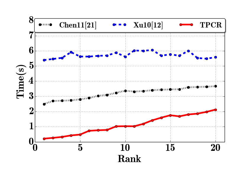
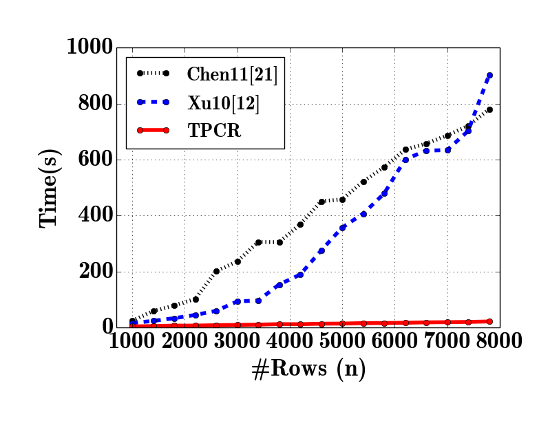
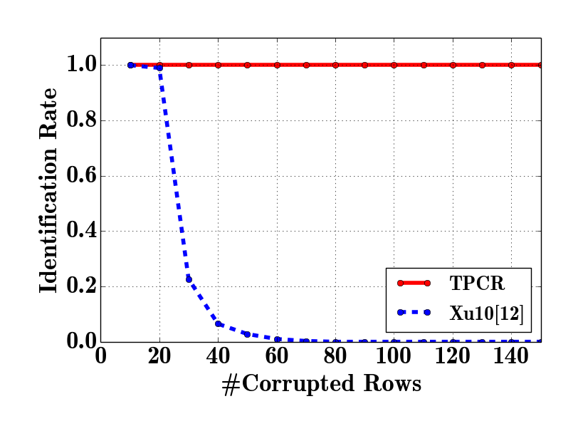
(a)	(b)	(c)

Figure 1: (a) Runtime, as a function of rank. (b) Runtime, as a function of the number of rows (n). (c) Rate of correct identification of corrupted rows.

Error on noisy data: We add noise to $\textbf{X}_{\star}$ to evaluate performance on noisy data. Since [21] cannot handle noise, we only compare with [12]. On each element of $\textbf{X}_{\star}$, we add a noise sampled from $\mathcal{N}(0,0.01)$. Figure 2(a) and 2(b) show RMSE of the difference from recovered $\textbf{X}^{\mathcal{O}}$ and the true $\textbf{X}_{\star}$. This metric is used by [12] as well. We use the grayscale to denote the RMSE: lighter color corresponds to smaller RMSE. On most test cases our algorithm successfully recovers the true subspace, while [12] fails on most cases. Particularly, when $n_{1}<120$, our approach can completely recover the underlying low-rank matrix. When $n_{1}$ increases, the condition $\mathit{SR}(\textbf{X}_{0})>\mathit{NR}(\textbf{X}_{0})$ might not hold true, and Theorem 3 says that no algorithm can recover the true subspace with probability greater than $1/2$. However, this theorem does not prevent our algorithm succeeding with probability $<1/2$, which is why we observe several white spots for high $n_{1}$.

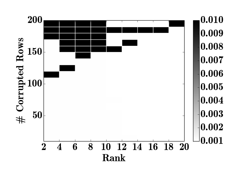
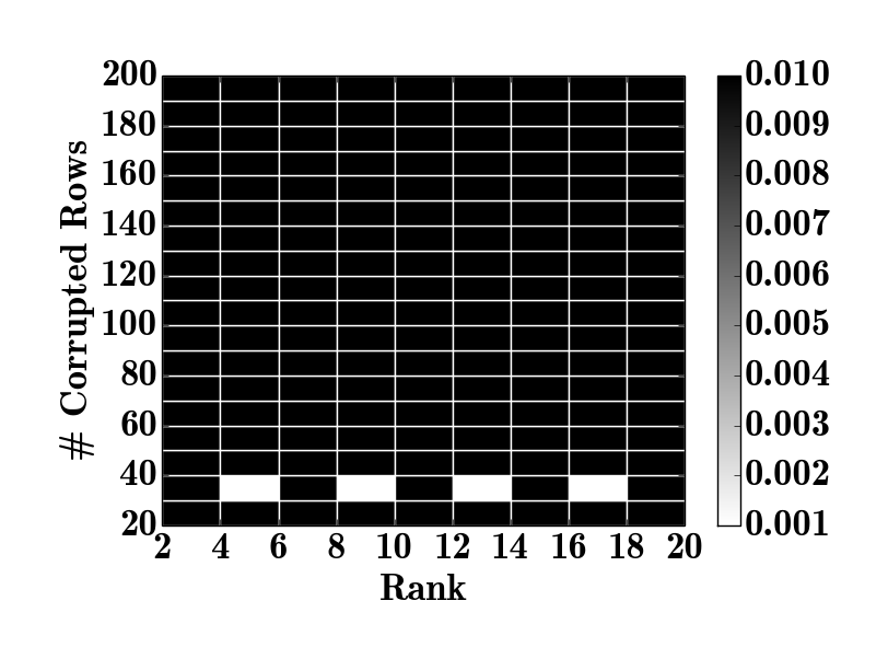
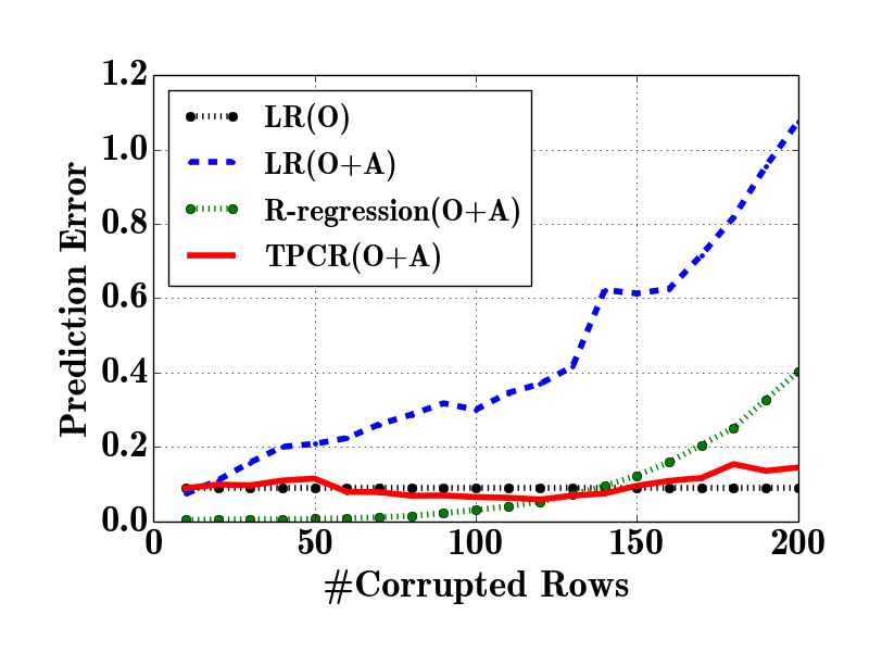
(a) TPCR	(b) Xu et al. [12]	(c)

Figure 2: (a) and (b) compares RMSE for T-PCR (a) and Xu et al. [12] (b). (c) RMSE comparison with robust regression (Chen et al. [9]) and non-robust baseline.

Robust Regression: We evaluate our T-PCR Algorithm 3 against the robust regression method of Chen et al. [9], which is the only alternative method for linear regression robust to adversarial data poisoning. As a baseline, we also present results for standard OLS linear regression with and without adversarial instances (LR(O+A) and LR(O), respectively). Results are evaluated using a ground truth test set not used for training. The results, shown in Figure 2(c), demonstrate that our algorithm significantly outperforms the alternatives. Indeed, while robust regression of Chen et al. [9] does better than the non-robust baseline, our method works nearly as well as linear regression without adversarial instances!

7 Conclusion

This paper considers the poisoning attack for linear regression problem with dimensionality reduction. We address the problem in two steps: 1) introducing a novel robust matrix factorization method to recover the true subspace, and 2) novel robust principle component regression to prune adversarial instances based on the basis recovered in step (1). We characterize necessary and sufficient conditions for our approach to be successful in recovering the true subspace, and present a bound on expected prediction loss compared to ground truth. Experimental results suggest that the proposed approach is extremely effective, and significantly outperforms prior art.

Appendix A Proof of Theorems in Section 3

Since, this section does not involve y, we will omit y without loss of clarity.

A.1 Theorem 1

Proof of Theorem 1.

We prove by contradiction. Assume we have a learner $\mathcal{L}_{\text{recover}}$, can solve Problem 1 with probability more than 1/2. We want to show that there exist two different spaces of rank-$k$, and one input X such that $\mathcal{L}_{\text{recover}}(\textbf{X}_{1})$ should return both two spaces with a probability $>1/2$, which is impossible. In the following, we construct such two spaces. Particularly, we will discuss how adversary can manipulate the matrix.

The adversary can choose $\mathcal{I}$ which maximize $|\mathcal{I}|$ such that while ${\mathrm{rank}(\textbf{X}_{\star}^{\mathcal{I}})}\leq k-1$. We know $|\mathcal{I}|=\mathit{MS}_{k-1}(\textbf{X}_{\star})\geq n-n_{1}$. This means that $|\mathcal{O}|-|\mathcal{I}|\leq n_{1}$.

Suppose $v_{1},...,v_{k-1}$ be a set of basis for the row space of $\textbf{X}_{\star}^{\mathcal{I}}$. The adversary then choose a vector $v_{k}^{\prime}$ which is orthogonal to $\textbf{X}_{\star}$. Then we know the span space of $V^{\prime}=\{v_{1},...,v_{k_{1}},v_{k}^{\prime}\}$ is different from $\textbf{X}_{\star}$. Then the adversary draws $n_{1}$ samples from the span space of $V^{\prime}$, and insert them into $\textbf{X}_{\star}$ to form X. Moreover, we denote $\textbf{X}_{\star}^{\prime}$ to be a matrix of $|\mathcal{I}|+n_{1}$ rows, so that the first $|\mathcal{I}|$ rows are $\textbf{X}_{\star}^{\mathcal{I}}$, and the rest $n_{1}$ rows sampled by the adversary. Therefore, we know $\textbf{X}_{\star}^{\prime}$ is also a submatrix of X, and we know that there are at most $|\mathcal{O}|-|\mathcal{I}|\leq n_{1}$ rows in X not coming from $\textbf{X}_{\star}^{\prime}$.

In doing so, we know that X is constructed by corrupting $\textbf{X}_{\star}$. On the other hand, we can also see X as the result of corrupting $\textbf{X}_{\star}^{\prime}$ by inserting $|\mathcal{O}|-|\mathcal{I}|\leq n_{1}$ rows. Therefore, $\mathcal{L}_{\text{recover}}(\textbf{X}_{\star})$ should return both $\textbf{X}_{\star}$ and $\textbf{X}_{\star}^{\prime}$ with a probability greater than $1/2$, which is impossible. Therefore, our conclusion holds true. ∎

A.2 Theorem 2

Proof of Theorem 2.

We show that Algorithm 1 recovers the subspace of $\textbf{X}_{\star}$ exactly. Assume B is returned by Algorithm 1 over X. We only need to show that B is a basis of $\textbf{X}_{\star}$. By Algorithm 1, we know that B is a basis of $n$ rows in $\mathcal{I}$ of X. Since we know any adversary can corrupt at most $n_{1}$ rows, thus $|\mathcal{I}\cap\mathcal{A}|\leq n_{1}$. Therefore, by combining the assumption $n_{1}+\mathit{MS}_{k-1}(\textbf{X}_{\star})<n$, we know that

$$|\mathcal{I}\cap\mathcal{O}|=|\mathcal{I}|-|\mathcal{I}\cap\mathcal{A}|\geq n-n_{1}>\mathit{MS}_{k-1}(\textbf{X}_{\star})$$ (7)

Therefore, we know B is a basis for $\textbf{X}_{\star}^{\mathcal{I}\cap\mathcal{O}}$. By the definition of $\mathit{MS}_{k-1}(\textbf{X}_{\star})$ and inequality (7), we know that

$${\mathrm{rank}(\textbf{X}_{\star}^{\mathcal{I}\cap\mathcal{O}})}=k$$

Therefore, we know that $\textbf{X}_{\star}^{\mathcal{I}\cap\mathcal{O}}$ is exactly the same subspace as $\textbf{X}_{\star}$, and thus B is the basis of $\textbf{X}_{\star}$. ∎

A.3 Corollary 1

Lemma 2.

$\mathit{MS}_{k-1}(\textbf{X}_{\star})\geq k-1$

Proof.

We can choose the $\mathcal{I}=\{1,...,k-1\}$, then we have ${\mathrm{rank}(\textbf{X}_{\star}^{\mathcal{I}})}\leq k-1$. Therefore, $\mathit{MS}_{k-1}(\textbf{X}_{\star})\geq|\mathcal{I}|=k-1$. ∎

Now, we can prove Corollary 1.

Proof of Corollary 1.

Given $\frac{n_{1}}{n}=\gamma\geq 1-\frac{k-1}{n}$, we have

$$n_{1}+(k-1)\geq n$$

Combining $\mathit{MS}_{k-1}(\textbf{X}_{\star})\geq k-1$, we know

$$n_{1}+\mathit{MS}_{k-1}(\textbf{X}_{\star})\geq n_{1}+(k-1)\geq n$$

Applying Theorem 1, we can conclude this corollary. ∎

A.4 Theorem 3

Proof of Theorem 3.

The proof of this theorem is similar to the proof of Theorem 1 and 2. First, when $\mathit{SR}(\textbf{X}_{0})\leq\mathit{NR}(\textbf{X}_{0})$, the adversary can construct X such that two subspaces should be recovered with a probability greater than $1/2$. Particularly, we assume $\mathcal{I},\textbf{U},\textbf{B}$ minimize objective  2, and thus $\mathit{SR}(\textbf{X}_{0})=||\textbf{X}_{0}^{\mathcal{I}}-\textbf{U}\textbf{B}||$. The adversary samples $n_{1}$ rows $\textbf{X}_{\text{corrupt}}$ from the span space of B, which does not belong to the span of $\textbf{X}_{\star}$. We add a small noise over $\textbf{X}_{\text{corrupt}}$ to get $\textbf{X}_{1}$, such that (1) $\textbf{X}_{\text{corrupt}}$ minimize $||\textbf{X}_{1}-\textbf{X}_{\text{corrupt}}||$; and (2) $||\textbf{X}_{1}-\textbf{X}_{\text{corrupt}}||=\mathit{NR}(\textbf{X}_{0})-\mathit{SR}(\textbf{X}_{0})$. Then the adversary insert $\textbf{X}_{1}$ into $\textbf{X}_{0}$ to get X. In this case, we know that $\textbf{X}_{\star}$ optimizes its distance from $\textbf{X}_{0}$, while the $[\textbf{X}_{\star}^{\mathcal{I}};\textbf{X}_{\text{corrupt}}]$ optimizes its distance from $[\textbf{X}_{0}^{\mathcal{I}};\textbf{X}_{\text{corrupt}}]$, where we use $[A;B]$ to denote the concatenation of rows from $A$ and $B$ respectively. Further, by definition, we know both of these two distances is $\mathit{NR}(\textbf{X}_{0})$. Therefore, the learner should recover from X both $\textbf{X}_{\star}$ and $[\textbf{X}_{0}^{\mathcal{I}};\textbf{X}_{\text{corrupt}}]$ with probability greater than $1/2$. This is impossible! Therefore the first part of the theorem holds true.

For the second part, we follow the proof of Theorem 2 verbatim, and present the difference. We show that Algorithm 2 recovers the subspace of $\textbf{X}_{\star}$ exactly. Assume B is returned by Algorithm 2 over X. We only need to show that B is a basis of $\textbf{X}_{\star}$. By Algorithm 2, we know that B optimizes its pan distance from a subset of $n$ rows in X, which is denoted as $\mathcal{I}$. Since we know any adversary can corrupt at most $n_{1}$ rows, thus $|\mathcal{I}\cap\mathcal{A}|\leq n_{1}$. Therefore, we know that

$$|\mathcal{I}\cap\mathcal{O}|=|\mathcal{I}|-|\mathcal{I}\cap\mathcal{A}|\geq n-n_{1}$$ (8)

If B is not a basis of $\textbf{X}_{\star}$, which means that $\textbf{X}_{\star}\textbf{B}^{T}\textbf{B}\neq\textbf{X}_{\star}$, then we know that the distance between the span space of B and $\textbf{X}^{\mathcal{I}\cap\mathcal{O}}$ is greater than $\mathit{SR}(\textbf{X}_{0})>\mathit{NR}(\textbf{X}_{0})$. This is impossible, since Algorithm 2 guarantees that this distance should be no greater than $\mathit{NR}(\textbf{X}_{0})$. Contradiction! Therefore the second part of the theorem holds true. ∎

A.5 Theorem 4

Proof of Theorem 4.

When $\textbf{N}=0$, we know that $\mathit{SR}(\textbf{X}_{0})>\mathit{NR}(\textbf{X}_{0})$ if and only if $\mathit{SR}(\textbf{X}_{0})\neq 0$. This means that for any $|\mathcal{I}|=n-n_{1}$, $\textbf{X}_{\star}^{\mathcal{I}}=\textbf{U}\textbf{B}$ implies that $\textbf{X}_{\star}\textbf{B}^{T}\textbf{B}=\textbf{X}_{\star}$ (condition (2b)), which implies that ${\mathrm{rank}(\textbf{X}_{\star}^{\mathcal{I}}|)}=k$ for all $\mathcal{I}$. Therefore, we know $\mathit{MS}_{k-1}(\textbf{X}_{\star})<n-n_{1}$, which concludes this theorem. ∎

Appendix B Proof of Lemma 5

Proof.

Assume                     $\beta_{U}$ $\textstyle\kern-0.6pt\bigwedge\kern-0.6pt$                      is the solution for this optimization problem. We assume the adversary wants to induce the regression system to compute                     $\beta_{U}$ $\textstyle\kern-0.6pt\bigwedge\kern-0.6pt$                     . In this case, he has to corrupt $\gamma n$ rows in $U$. W.L.O.G. we can assume $\mathcal{O}=\{1,...,n_{1}\}$. We denote $\beta_{U}^{\star}=\textbf{B}\beta^{\star}$. Since $\textbf{X}_{\star}=\textbf{U}_{\star}\textbf{B}$, we know that

$$\textbf{y}-\textbf{X}_{\star}\beta^{\star}=\textbf{y}-\textbf{U}_{\star}\beta_{U}^{\star}$$

Since                     $\beta_{U}$ $\textstyle\kern-0.6pt\bigwedge\kern-0.6pt$                      optimize Eq (4), we assume $(y_{i}-u_{i}\leavevmode\hbox{\set@color\hskip 66.6052pt\leavevmode\hbox{\set@color$\beta_{U}$}\raisebox{9.858pt}{$\leavevmode\hbox{\set@color\raisebox{-0.95679pt}{\leavevmode\resizebox{133.2104pt}{1.19598pt}{\leavevmode\hbox{\set@color$\mathchoice{\raisebox{-112.41994pt}{\leavevmode\resizebox{40.36137pt}{393.47006pt}{\leavevmode\hbox{\set@color$\displaystyle\mathchoice{\raisebox{0.0pt}{\leavevmode\resizebox{10.09035pt}{393.47pt}{\leavevmode\hbox{\set@color$\displaystyle\kern-0.6pt\bigwedge\kern-0.6pt$}}}}{\raisebox{0.0pt}{\leavevmode\resizebox{10.09035pt}{393.47pt}{\leavevmode\hbox{\set@color$\textstyle\kern-0.6pt\bigwedge\kern-0.6pt$}}}}{\raisebox{0.0pt}{\leavevmode\resizebox{10.09035pt}{393.47028pt}{\leavevmode\hbox{\set@color$\scriptstyle\kern-0.6pt\bigwedge\kern-0.6pt$}}}}{\raisebox{0.0pt}{\leavevmode\resizebox{10.09035pt}{393.47pt}{\leavevmode\hbox{\set@color$\scriptscriptstyle\kern-0.6pt\bigwedge\kern-0.6pt$}}}}$}}}}{\raisebox{-112.41994pt}{\leavevmode\resizebox{40.36137pt}{393.47006pt}{\leavevmode\hbox{\set@color$\textstyle\mathchoice{\raisebox{0.0pt}{\leavevmode\resizebox{10.09035pt}{393.47pt}{\leavevmode\hbox{\set@color$\displaystyle\kern-0.6pt\bigwedge\kern-0.6pt$}}}}{\raisebox{0.0pt}{\leavevmode\resizebox{10.09035pt}{393.47pt}{\leavevmode\hbox{\set@color$\textstyle\kern-0.6pt\bigwedge\kern-0.6pt$}}}}{\raisebox{0.0pt}{\leavevmode\resizebox{10.09035pt}{393.47028pt}{\leavevmode\hbox{\set@color$\scriptstyle\kern-0.6pt\bigwedge\kern-0.6pt$}}}}{\raisebox{0.0pt}{\leavevmode\resizebox{10.09035pt}{393.47pt}{\leavevmode\hbox{\set@color$\scriptscriptstyle\kern-0.6pt\bigwedge\kern-0.6pt$}}}}$}}}}{\raisebox{-112.41978pt}{\leavevmode\resizebox{28.50635pt}{393.47021pt}{\leavevmode\hbox{\set@color$\scriptstyle\mathchoice{\raisebox{0.0pt}{\leavevmode\resizebox{7.12659pt}{393.47028pt}{\leavevmode\hbox{\set@color$\displaystyle\kern-0.6pt\bigwedge\kern-0.6pt$}}}}{\raisebox{0.0pt}{\leavevmode\resizebox{7.12659pt}{393.47028pt}{\leavevmode\hbox{\set@color$\textstyle\kern-0.6pt\bigwedge\kern-0.6pt$}}}}{\raisebox{0.0pt}{\leavevmode\resizebox{7.12659pt}{393.4702pt}{\leavevmode\hbox{\set@color$\scriptstyle\kern-0.6pt\bigwedge\kern-0.6pt$}}}}{\raisebox{0.0pt}{\leavevmode\resizebox{7.12659pt}{393.47028pt}{\leavevmode\hbox{\set@color$\scriptscriptstyle\kern-0.6pt\bigwedge\kern-0.6pt$}}}}$}}}}{\raisebox{-112.41994pt}{\leavevmode\resizebox{23.98131pt}{393.47006pt}{\leavevmode\hbox{\set@color$\scriptscriptstyle\mathchoice{\raisebox{0.0pt}{\leavevmode\resizebox{5.99533pt}{393.47pt}{\leavevmode\hbox{\set@color$\displaystyle\kern-0.6pt\bigwedge\kern-0.6pt$}}}}{\raisebox{0.0pt}{\leavevmode\resizebox{5.99533pt}{393.47pt}{\leavevmode\hbox{\set@color$\textstyle\kern-0.6pt\bigwedge\kern-0.6pt$}}}}{\raisebox{0.0pt}{\leavevmode\resizebox{5.99533pt}{393.47028pt}{\leavevmode\hbox{\set@color$\scriptstyle\kern-0.6pt\bigwedge\kern-0.6pt$}}}}{\raisebox{0.0pt}{\leavevmode\resizebox{5.99533pt}{393.47pt}{\leavevmode\hbox{\set@color$\scriptscriptstyle\kern-0.6pt\bigwedge\kern-0.6pt$}}}}$}}}}$}}}}$}\hskip 66.6052pt})^{2}$ are the smallest $n$ values for $i\in\{1,...,n\}$.

Then we have

$$\sum_{i=1}^{n_{1}}(y_{i}-u_{i}\leavevmode\hbox{\set@color\hskip 66.6052pt\leavevmode\hbox{\set@color$\beta_{U}$}\raisebox{9.858pt}{$\leavevmode\hbox{\set@color\raisebox{-0.95679pt}{\leavevmode\resizebox{133.2104pt}{1.19598pt}{\leavevmode\hbox{\set@color$\mathchoice{\raisebox{-112.41994pt}{\leavevmode\resizebox{40.36137pt}{393.47006pt}{\leavevmode\hbox{\set@color$\displaystyle\mathchoice{\raisebox{0.0pt}{\leavevmode\resizebox{10.09035pt}{393.47pt}{\leavevmode\hbox{\set@color$\displaystyle\kern-0.6pt\bigwedge\kern-0.6pt$}}}}{\raisebox{0.0pt}{\leavevmode\resizebox{10.09035pt}{393.47pt}{\leavevmode\hbox{\set@color$\textstyle\kern-0.6pt\bigwedge\kern-0.6pt$}}}}{\raisebox{0.0pt}{\leavevmode\resizebox{10.09035pt}{393.47028pt}{\leavevmode\hbox{\set@color$\scriptstyle\kern-0.6pt\bigwedge\kern-0.6pt$}}}}{\raisebox{0.0pt}{\leavevmode\resizebox{10.09035pt}{393.47pt}{\leavevmode\hbox{\set@color$\scriptscriptstyle\kern-0.6pt\bigwedge\kern-0.6pt$}}}}$}}}}{\raisebox{-112.41994pt}{\leavevmode\resizebox{40.36137pt}{393.47006pt}{\leavevmode\hbox{\set@color$\textstyle\mathchoice{\raisebox{0.0pt}{\leavevmode\resizebox{10.09035pt}{393.47pt}{\leavevmode\hbox{\set@color$\displaystyle\kern-0.6pt\bigwedge\kern-0.6pt$}}}}{\raisebox{0.0pt}{\leavevmode\resizebox{10.09035pt}{393.47pt}{\leavevmode\hbox{\set@color$\textstyle\kern-0.6pt\bigwedge\kern-0.6pt$}}}}{\raisebox{0.0pt}{\leavevmode\resizebox{10.09035pt}{393.47028pt}{\leavevmode\hbox{\set@color$\scriptstyle\kern-0.6pt\bigwedge\kern-0.6pt$}}}}{\raisebox{0.0pt}{\leavevmode\resizebox{10.09035pt}{393.47pt}{\leavevmode\hbox{\set@color$\scriptscriptstyle\kern-0.6pt\bigwedge\kern-0.6pt$}}}}$}}}}{\raisebox{-112.41978pt}{\leavevmode\resizebox{28.50635pt}{393.47021pt}{\leavevmode\hbox{\set@color$\scriptstyle\mathchoice{\raisebox{0.0pt}{\leavevmode\resizebox{7.12659pt}{393.47028pt}{\leavevmode\hbox{\set@color$\displaystyle\kern-0.6pt\bigwedge\kern-0.6pt$}}}}{\raisebox{0.0pt}{\leavevmode\resizebox{7.12659pt}{393.47028pt}{\leavevmode\hbox{\set@color$\textstyle\kern-0.6pt\bigwedge\kern-0.6pt$}}}}{\raisebox{0.0pt}{\leavevmode\resizebox{7.12659pt}{393.4702pt}{\leavevmode\hbox{\set@color$\scriptstyle\kern-0.6pt\bigwedge\kern-0.6pt$}}}}{\raisebox{0.0pt}{\leavevmode\resizebox{7.12659pt}{393.47028pt}{\leavevmode\hbox{\set@color$\scriptscriptstyle\kern-0.6pt\bigwedge\kern-0.6pt$}}}}$}}}}{\raisebox{-112.41994pt}{\leavevmode\resizebox{23.98131pt}{393.47006pt}{\leavevmode\hbox{\set@color$\scriptscriptstyle\mathchoice{\raisebox{0.0pt}{\leavevmode\resizebox{5.99533pt}{393.47pt}{\leavevmode\hbox{\set@color$\displaystyle\kern-0.6pt\bigwedge\kern-0.6pt$}}}}{\raisebox{0.0pt}{\leavevmode\resizebox{5.99533pt}{393.47pt}{\leavevmode\hbox{\set@color$\textstyle\kern-0.6pt\bigwedge\kern-0.6pt$}}}}{\raisebox{0.0pt}{\leavevmode\resizebox{5.99533pt}{393.47028pt}{\leavevmode\hbox{\set@color$\scriptstyle\kern-0.6pt\bigwedge\kern-0.6pt$}}}}{\raisebox{0.0pt}{\leavevmode\resizebox{5.99533pt}{393.47pt}{\leavevmode\hbox{\set@color$\scriptscriptstyle\kern-0.6pt\bigwedge\kern-0.6pt$}}}}$}}}}$}}}}$}\hskip 66.6052pt})^{2}+\sum_{i=n_{1}+1}^{n}(y_{i}-u_{i}\leavevmode\hbox{\set@color\hskip 66.6052pt\leavevmode\hbox{\set@color$\beta_{U}$}\raisebox{9.858pt}{$\leavevmode\hbox{\set@color\raisebox{-0.95679pt}{\leavevmode\resizebox{133.2104pt}{1.19598pt}{\leavevmode\hbox{\set@color$\mathchoice{\raisebox{-112.41994pt}{\leavevmode\resizebox{40.36137pt}{393.47006pt}{\leavevmode\hbox{\set@color$\displaystyle\mathchoice{\raisebox{0.0pt}{\leavevmode\resizebox{10.09035pt}{393.47pt}{\leavevmode\hbox{\set@color$\displaystyle\kern-0.6pt\bigwedge\kern-0.6pt$}}}}{\raisebox{0.0pt}{\leavevmode\resizebox{10.09035pt}{393.47pt}{\leavevmode\hbox{\set@color$\textstyle\kern-0.6pt\bigwedge\kern-0.6pt$}}}}{\raisebox{0.0pt}{\leavevmode\resizebox{10.09035pt}{393.47028pt}{\leavevmode\hbox{\set@color$\scriptstyle\kern-0.6pt\bigwedge\kern-0.6pt$}}}}{\raisebox{0.0pt}{\leavevmode\resizebox{10.09035pt}{393.47pt}{\leavevmode\hbox{\set@color$\scriptscriptstyle\kern-0.6pt\bigwedge\kern-0.6pt$}}}}$}}}}{\raisebox{-112.41994pt}{\leavevmode\resizebox{40.36137pt}{393.47006pt}{\leavevmode\hbox{\set@color$\textstyle\mathchoice{\raisebox{0.0pt}{\leavevmode\resizebox{10.09035pt}{393.47pt}{\leavevmode\hbox{\set@color$\displaystyle\kern-0.6pt\bigwedge\kern-0.6pt$}}}}{\raisebox{0.0pt}{\leavevmode\resizebox{10.09035pt}{393.47pt}{\leavevmode\hbox{\set@color$\textstyle\kern-0.6pt\bigwedge\kern-0.6pt$}}}}{\raisebox{0.0pt}{\leavevmode\resizebox{10.09035pt}{393.47028pt}{\leavevmode\hbox{\set@color$\scriptstyle\kern-0.6pt\bigwedge\kern-0.6pt$}}}}{\raisebox{0.0pt}{\leavevmode\resizebox{10.09035pt}{393.47pt}{\leavevmode\hbox{\set@color$\scriptscriptstyle\kern-0.6pt\bigwedge\kern-0.6pt$}}}}$}}}}{\raisebox{-112.41978pt}{\leavevmode\resizebox{28.50635pt}{393.47021pt}{\leavevmode\hbox{\set@color$\scriptstyle\mathchoice{\raisebox{0.0pt}{\leavevmode\resizebox{7.12659pt}{393.47028pt}{\leavevmode\hbox{\set@color$\displaystyle\kern-0.6pt\bigwedge\kern-0.6pt$}}}}{\raisebox{0.0pt}{\leavevmode\resizebox{7.12659pt}{393.47028pt}{\leavevmode\hbox{\set@color$\textstyle\kern-0.6pt\bigwedge\kern-0.6pt$}}}}{\raisebox{0.0pt}{\leavevmode\resizebox{7.12659pt}{393.4702pt}{\leavevmode\hbox{\set@color$\scriptstyle\kern-0.6pt\bigwedge\kern-0.6pt$}}}}{\raisebox{0.0pt}{\leavevmode\resizebox{7.12659pt}{393.47028pt}{\leavevmode\hbox{\set@color$\scriptscriptstyle\kern-0.6pt\bigwedge\kern-0.6pt$}}}}$}}}}{\raisebox{-112.41994pt}{\leavevmode\resizebox{23.98131pt}{393.47006pt}{\leavevmode\hbox{\set@color$\scriptscriptstyle\mathchoice{\raisebox{0.0pt}{\leavevmode\resizebox{5.99533pt}{393.47pt}{\leavevmode\hbox{\set@color$\displaystyle\kern-0.6pt\bigwedge\kern-0.6pt$}}}}{\raisebox{0.0pt}{\leavevmode\resizebox{5.99533pt}{393.47pt}{\leavevmode\hbox{\set@color$\textstyle\kern-0.6pt\bigwedge\kern-0.6pt$}}}}{\raisebox{0.0pt}{\leavevmode\resizebox{5.99533pt}{393.47028pt}{\leavevmode\hbox{\set@color$\scriptstyle\kern-0.6pt\bigwedge\kern-0.6pt$}}}}{\raisebox{0.0pt}{\leavevmode\resizebox{5.99533pt}{393.47pt}{\leavevmode\hbox{\set@color$\scriptscriptstyle\kern-0.6pt\bigwedge\kern-0.6pt$}}}}$}}}}$}}}}$}\hskip 66.6052pt})^{2}\leq\sum_{i=n_{1}+1}^{n+n_{1}}(y_{i}-u_{i}^{T}\beta_{U}^{\star})^{2}$$

Therefore we have

$$\sum_{i=n_{1}+1}^{n}(y_{i}-u_{i}\leavevmode\hbox{\set@color\hskip 66.6052pt\leavevmode\hbox{\set@color$\beta_{U}$}\raisebox{9.858pt}{$\leavevmode\hbox{\set@color\raisebox{-0.95679pt}{\leavevmode\resizebox{133.2104pt}{1.19598pt}{\leavevmode\hbox{\set@color$\mathchoice{\raisebox{-112.41994pt}{\leavevmode\resizebox{40.36137pt}{393.47006pt}{\leavevmode\hbox{\set@color$\displaystyle\mathchoice{\raisebox{0.0pt}{\leavevmode\resizebox{10.09035pt}{393.47pt}{\leavevmode\hbox{\set@color$\displaystyle\kern-0.6pt\bigwedge\kern-0.6pt$}}}}{\raisebox{0.0pt}{\leavevmode\resizebox{10.09035pt}{393.47pt}{\leavevmode\hbox{\set@color$\textstyle\kern-0.6pt\bigwedge\kern-0.6pt$}}}}{\raisebox{0.0pt}{\leavevmode\resizebox{10.09035pt}{393.47028pt}{\leavevmode\hbox{\set@color$\scriptstyle\kern-0.6pt\bigwedge\kern-0.6pt$}}}}{\raisebox{0.0pt}{\leavevmode\resizebox{10.09035pt}{393.47pt}{\leavevmode\hbox{\set@color$\scriptscriptstyle\kern-0.6pt\bigwedge\kern-0.6pt$}}}}$}}}}{\raisebox{-112.41994pt}{\leavevmode\resizebox{40.36137pt}{393.47006pt}{\leavevmode\hbox{\set@color$\textstyle\mathchoice{\raisebox{0.0pt}{\leavevmode\resizebox{10.09035pt}{393.47pt}{\leavevmode\hbox{\set@color$\displaystyle\kern-0.6pt\bigwedge\kern-0.6pt$}}}}{\raisebox{0.0pt}{\leavevmode\resizebox{10.09035pt}{393.47pt}{\leavevmode\hbox{\set@color$\textstyle\kern-0.6pt\bigwedge\kern-0.6pt$}}}}{\raisebox{0.0pt}{\leavevmode\resizebox{10.09035pt}{393.47028pt}{\leavevmode\hbox{\set@color$\scriptstyle\kern-0.6pt\bigwedge\kern-0.6pt$}}}}{\raisebox{0.0pt}{\leavevmode\resizebox{10.09035pt}{393.47pt}{\leavevmode\hbox{\set@color$\scriptscriptstyle\kern-0.6pt\bigwedge\kern-0.6pt$}}}}$}}}}{\raisebox{-112.41978pt}{\leavevmode\resizebox{28.50635pt}{393.47021pt}{\leavevmode\hbox{\set@color$\scriptstyle\mathchoice{\raisebox{0.0pt}{\leavevmode\resizebox{7.12659pt}{393.47028pt}{\leavevmode\hbox{\set@color$\displaystyle\kern-0.6pt\bigwedge\kern-0.6pt$}}}}{\raisebox{0.0pt}{\leavevmode\resizebox{7.12659pt}{393.47028pt}{\leavevmode\hbox{\set@color$\textstyle\kern-0.6pt\bigwedge\kern-0.6pt$}}}}{\raisebox{0.0pt}{\leavevmode\resizebox{7.12659pt}{393.4702pt}{\leavevmode\hbox{\set@color$\scriptstyle\kern-0.6pt\bigwedge\kern-0.6pt$}}}}{\raisebox{0.0pt}{\leavevmode\resizebox{7.12659pt}{393.47028pt}{\leavevmode\hbox{\set@color$\scriptscriptstyle\kern-0.6pt\bigwedge\kern-0.6pt$}}}}$}}}}{\raisebox{-112.41994pt}{\leavevmode\resizebox{23.98131pt}{393.47006pt}{\leavevmode\hbox{\set@color$\scriptscriptstyle\mathchoice{\raisebox{0.0pt}{\leavevmode\resizebox{5.99533pt}{393.47pt}{\leavevmode\hbox{\set@color$\displaystyle\kern-0.6pt\bigwedge\kern-0.6pt$}}}}{\raisebox{0.0pt}{\leavevmode\resizebox{5.99533pt}{393.47pt}{\leavevmode\hbox{\set@color$\textstyle\kern-0.6pt\bigwedge\kern-0.6pt$}}}}{\raisebox{0.0pt}{\leavevmode\resizebox{5.99533pt}{393.47028pt}{\leavevmode\hbox{\set@color$\scriptstyle\kern-0.6pt\bigwedge\kern-0.6pt$}}}}{\raisebox{0.0pt}{\leavevmode\resizebox{5.99533pt}{393.47pt}{\leavevmode\hbox{\set@color$\scriptscriptstyle\kern-0.6pt\bigwedge\kern-0.6pt$}}}}$}}}}$}}}}$}\hskip 66.6052pt})^{2}\leq\sum_{i=n_{1}+1}^{n+n_{1}}(y_{i}-u_{i}\beta_{U}^{\star})^{2}$$ (9)

Further, we know

$$\sum_{i=n_{1}+1}^{n}(y_{i}-u_{i}\leavevmode\hbox{\set@color\hskip 66.6052pt\leavevmode\hbox{\set@color$\beta_{U}$}\raisebox{9.858pt}{$\leavevmode\hbox{\set@color\raisebox{-0.95679pt}{\leavevmode\resizebox{133.2104pt}{1.19598pt}{\leavevmode\hbox{\set@color$\mathchoice{\raisebox{-112.41994pt}{\leavevmode\resizebox{40.36137pt}{393.47006pt}{\leavevmode\hbox{\set@color$\displaystyle\mathchoice{\raisebox{0.0pt}{\leavevmode\resizebox{10.09035pt}{393.47pt}{\leavevmode\hbox{\set@color$\displaystyle\kern-0.6pt\bigwedge\kern-0.6pt$}}}}{\raisebox{0.0pt}{\leavevmode\resizebox{10.09035pt}{393.47pt}{\leavevmode\hbox{\set@color$\textstyle\kern-0.6pt\bigwedge\kern-0.6pt$}}}}{\raisebox{0.0pt}{\leavevmode\resizebox{10.09035pt}{393.47028pt}{\leavevmode\hbox{\set@color$\scriptstyle\kern-0.6pt\bigwedge\kern-0.6pt$}}}}{\raisebox{0.0pt}{\leavevmode\resizebox{10.09035pt}{393.47pt}{\leavevmode\hbox{\set@color$\scriptscriptstyle\kern-0.6pt\bigwedge\kern-0.6pt$}}}}$}}}}{\raisebox{-112.41994pt}{\leavevmode\resizebox{40.36137pt}{393.47006pt}{\leavevmode\hbox{\set@color$\textstyle\mathchoice{\raisebox{0.0pt}{\leavevmode\resizebox{10.09035pt}{393.47pt}{\leavevmode\hbox{\set@color$\displaystyle\kern-0.6pt\bigwedge\kern-0.6pt$}}}}{\raisebox{0.0pt}{\leavevmode\resizebox{10.09035pt}{393.47pt}{\leavevmode\hbox{\set@color$\textstyle\kern-0.6pt\bigwedge\kern-0.6pt$}}}}{\raisebox{0.0pt}{\leavevmode\resizebox{10.09035pt}{393.47028pt}{\leavevmode\hbox{\set@color$\scriptstyle\kern-0.6pt\bigwedge\kern-0.6pt$}}}}{\raisebox{0.0pt}{\leavevmode\resizebox{10.09035pt}{393.47pt}{\leavevmode\hbox{\set@color$\scriptscriptstyle\kern-0.6pt\bigwedge\kern-0.6pt$}}}}$}}}}{\raisebox{-112.41978pt}{\leavevmode\resizebox{28.50635pt}{393.47021pt}{\leavevmode\hbox{\set@color$\scriptstyle\mathchoice{\raisebox{0.0pt}{\leavevmode\resizebox{7.12659pt}{393.47028pt}{\leavevmode\hbox{\set@color$\displaystyle\kern-0.6pt\bigwedge\kern-0.6pt$}}}}{\raisebox{0.0pt}{\leavevmode\resizebox{7.12659pt}{393.47028pt}{\leavevmode\hbox{\set@color$\textstyle\kern-0.6pt\bigwedge\kern-0.6pt$}}}}{\raisebox{0.0pt}{\leavevmode\resizebox{7.12659pt}{393.4702pt}{\leavevmode\hbox{\set@color$\scriptstyle\kern-0.6pt\bigwedge\kern-0.6pt$}}}}{\raisebox{0.0pt}{\leavevmode\resizebox{7.12659pt}{393.47028pt}{\leavevmode\hbox{\set@color$\scriptscriptstyle\kern-0.6pt\bigwedge\kern-0.6pt$}}}}$}}}}{\raisebox{-112.41994pt}{\leavevmode\resizebox{23.98131pt}{393.47006pt}{\leavevmode\hbox{\set@color$\scriptscriptstyle\mathchoice{\raisebox{0.0pt}{\leavevmode\resizebox{5.99533pt}{393.47pt}{\leavevmode\hbox{\set@color$\displaystyle\kern-0.6pt\bigwedge\kern-0.6pt$}}}}{\raisebox{0.0pt}{\leavevmode\resizebox{5.99533pt}{393.47pt}{\leavevmode\hbox{\set@color$\textstyle\kern-0.6pt\bigwedge\kern-0.6pt$}}}}{\raisebox{0.0pt}{\leavevmode\resizebox{5.99533pt}{393.47028pt}{\leavevmode\hbox{\set@color$\scriptstyle\kern-0.6pt\bigwedge\kern-0.6pt$}}}}{\raisebox{0.0pt}{\leavevmode\resizebox{5.99533pt}{393.47pt}{\leavevmode\hbox{\set@color$\scriptscriptstyle\kern-0.6pt\bigwedge\kern-0.6pt$}}}}$}}}}$}}}}$}\hskip 66.6052pt})^{2}$$ (10)

$$= \sum_{i=n_{1}+1}^{n}\bigg{(}(y_{i}-u_{i}\beta_{U}^{\star})+(u_{i}\beta_{U}^{\star}-u_{i}\leavevmode\hbox{\set@color\hskip 66.6052pt\leavevmode\hbox{\set@color$\beta_{U}$}\raisebox{9.858pt}{$\leavevmode\hbox{\set@color\raisebox{-0.95679pt}{\leavevmode\resizebox{133.2104pt}{1.19598pt}{\leavevmode\hbox{\set@color$\mathchoice{\raisebox{-112.41994pt}{\leavevmode\resizebox{40.36137pt}{393.47006pt}{\leavevmode\hbox{\set@color$\displaystyle\mathchoice{\raisebox{0.0pt}{\leavevmode\resizebox{10.09035pt}{393.47pt}{\leavevmode\hbox{\set@color$\displaystyle\kern-0.6pt\bigwedge\kern-0.6pt$}}}}{\raisebox{0.0pt}{\leavevmode\resizebox{10.09035pt}{393.47pt}{\leavevmode\hbox{\set@color$\textstyle\kern-0.6pt\bigwedge\kern-0.6pt$}}}}{\raisebox{0.0pt}{\leavevmode\resizebox{10.09035pt}{393.47028pt}{\leavevmode\hbox{\set@color$\scriptstyle\kern-0.6pt\bigwedge\kern-0.6pt$}}}}{\raisebox{0.0pt}{\leavevmode\resizebox{10.09035pt}{393.47pt}{\leavevmode\hbox{\set@color$\scriptscriptstyle\kern-0.6pt\bigwedge\kern-0.6pt$}}}}$}}}}{\raisebox{-112.41994pt}{\leavevmode\resizebox{40.36137pt}{393.47006pt}{\leavevmode\hbox{\set@color$\textstyle\mathchoice{\raisebox{0.0pt}{\leavevmode\resizebox{10.09035pt}{393.47pt}{\leavevmode\hbox{\set@color$\displaystyle\kern-0.6pt\bigwedge\kern-0.6pt$}}}}{\raisebox{0.0pt}{\leavevmode\resizebox{10.09035pt}{393.47pt}{\leavevmode\hbox{\set@color$\textstyle\kern-0.6pt\bigwedge\kern-0.6pt$}}}}{\raisebox{0.0pt}{\leavevmode\resizebox{10.09035pt}{393.47028pt}{\leavevmode\hbox{\set@color$\scriptstyle\kern-0.6pt\bigwedge\kern-0.6pt$}}}}{\raisebox{0.0pt}{\leavevmode\resizebox{10.09035pt}{393.47pt}{\leavevmode\hbox{\set@color$\scriptscriptstyle\kern-0.6pt\bigwedge\kern-0.6pt$}}}}$}}}}{\raisebox{-112.41978pt}{\leavevmode\resizebox{28.50635pt}{393.47021pt}{\leavevmode\hbox{\set@color$\scriptstyle\mathchoice{\raisebox{0.0pt}{\leavevmode\resizebox{7.12659pt}{393.47028pt}{\leavevmode\hbox{\set@color$\displaystyle\kern-0.6pt\bigwedge\kern-0.6pt$}}}}{\raisebox{0.0pt}{\leavevmode\resizebox{7.12659pt}{393.47028pt}{\leavevmode\hbox{\set@color$\textstyle\kern-0.6pt\bigwedge\kern-0.6pt$}}}}{\raisebox{0.0pt}{\leavevmode\resizebox{7.12659pt}{393.4702pt}{\leavevmode\hbox{\set@color$\scriptstyle\kern-0.6pt\bigwedge\kern-0.6pt$}}}}{\raisebox{0.0pt}{\leavevmode\resizebox{7.12659pt}{393.47028pt}{\leavevmode\hbox{\set@color$\scriptscriptstyle\kern-0.6pt\bigwedge\kern-0.6pt$}}}}$}}}}{\raisebox{-112.41994pt}{\leavevmode\resizebox{23.98131pt}{393.47006pt}{\leavevmode\hbox{\set@color$\scriptscriptstyle\mathchoice{\raisebox{0.0pt}{\leavevmode\resizebox{5.99533pt}{393.47pt}{\leavevmode\hbox{\set@color$\displaystyle\kern-0.6pt\bigwedge\kern-0.6pt$}}}}{\raisebox{0.0pt}{\leavevmode\resizebox{5.99533pt}{393.47pt}{\leavevmode\hbox{\set@color$\textstyle\kern-0.6pt\bigwedge\kern-0.6pt$}}}}{\raisebox{0.0pt}{\leavevmode\resizebox{5.99533pt}{393.47028pt}{\leavevmode\hbox{\set@color$\scriptstyle\kern-0.6pt\bigwedge\kern-0.6pt$}}}}{\raisebox{0.0pt}{\leavevmode\resizebox{5.99533pt}{393.47pt}{\leavevmode\hbox{\set@color$\scriptscriptstyle\kern-0.6pt\bigwedge\kern-0.6pt$}}}}$}}}}$}}}}$}\hskip 66.6052pt})\bigg{)}^{2}$$

$$\geq \sum_{i=n_{1}+1}^{n}\bigg{\{}(y_{i}-u_{i}\beta_{U}^{\star})^{2}+(u_{i}\beta_{U}^{\star}-u_{i}\leavevmode\hbox{\set@color\hskip 66.6052pt\leavevmode\hbox{\set@color$\beta_{U}$}\raisebox{9.858pt}{$\leavevmode\hbox{\set@color\raisebox{-0.95679pt}{\leavevmode\resizebox{133.2104pt}{1.19598pt}{\leavevmode\hbox{\set@color$\mathchoice{\raisebox{-112.41994pt}{\leavevmode\resizebox{40.36137pt}{393.47006pt}{\leavevmode\hbox{\set@color$\displaystyle\mathchoice{\raisebox{0.0pt}{\leavevmode\resizebox{10.09035pt}{393.47pt}{\leavevmode\hbox{\set@color$\displaystyle\kern-0.6pt\bigwedge\kern-0.6pt$}}}}{\raisebox{0.0pt}{\leavevmode\resizebox{10.09035pt}{393.47pt}{\leavevmode\hbox{\set@color$\textstyle\kern-0.6pt\bigwedge\kern-0.6pt$}}}}{\raisebox{0.0pt}{\leavevmode\resizebox{10.09035pt}{393.47028pt}{\leavevmode\hbox{\set@color$\scriptstyle\kern-0.6pt\bigwedge\kern-0.6pt$}}}}{\raisebox{0.0pt}{\leavevmode\resizebox{10.09035pt}{393.47pt}{\leavevmode\hbox{\set@color$\scriptscriptstyle\kern-0.6pt\bigwedge\kern-0.6pt$}}}}$}}}}{\raisebox{-112.41994pt}{\leavevmode\resizebox{40.36137pt}{393.47006pt}{\leavevmode\hbox{\set@color$\textstyle\mathchoice{\raisebox{0.0pt}{\leavevmode\resizebox{10.09035pt}{393.47pt}{\leavevmode\hbox{\set@color$\displaystyle\kern-0.6pt\bigwedge\kern-0.6pt$}}}}{\raisebox{0.0pt}{\leavevmode\resizebox{10.09035pt}{393.47pt}{\leavevmode\hbox{\set@color$\textstyle\kern-0.6pt\bigwedge\kern-0.6pt$}}}}{\raisebox{0.0pt}{\leavevmode\resizebox{10.09035pt}{393.47028pt}{\leavevmode\hbox{\set@color$\scriptstyle\kern-0.6pt\bigwedge\kern-0.6pt$}}}}{\raisebox{0.0pt}{\leavevmode\resizebox{10.09035pt}{393.47pt}{\leavevmode\hbox{\set@color$\scriptscriptstyle\kern-0.6pt\bigwedge\kern-0.6pt$}}}}$}}}}{\raisebox{-112.41978pt}{\leavevmode\resizebox{28.50635pt}{393.47021pt}{\leavevmode\hbox{\set@color$\scriptstyle\mathchoice{\raisebox{0.0pt}{\leavevmode\resizebox{7.12659pt}{393.47028pt}{\leavevmode\hbox{\set@color$\displaystyle\kern-0.6pt\bigwedge\kern-0.6pt$}}}}{\raisebox{0.0pt}{\leavevmode\resizebox{7.12659pt}{393.47028pt}{\leavevmode\hbox{\set@color$\textstyle\kern-0.6pt\bigwedge\kern-0.6pt$}}}}{\raisebox{0.0pt}{\leavevmode\resizebox{7.12659pt}{393.4702pt}{\leavevmode\hbox{\set@color$\scriptstyle\kern-0.6pt\bigwedge\kern-0.6pt$}}}}{\raisebox{0.0pt}{\leavevmode\resizebox{7.12659pt}{393.47028pt}{\leavevmode\hbox{\set@color$\scriptscriptstyle\kern-0.6pt\bigwedge\kern-0.6pt$}}}}$}}}}{\raisebox{-112.41994pt}{\leavevmode\resizebox{23.98131pt}{393.47006pt}{\leavevmode\hbox{\set@color$\scriptscriptstyle\mathchoice{\raisebox{0.0pt}{\leavevmode\resizebox{5.99533pt}{393.47pt}{\leavevmode\hbox{\set@color$\displaystyle\kern-0.6pt\bigwedge\kern-0.6pt$}}}}{\raisebox{0.0pt}{\leavevmode\resizebox{5.99533pt}{393.47pt}{\leavevmode\hbox{\set@color$\textstyle\kern-0.6pt\bigwedge\kern-0.6pt$}}}}{\raisebox{0.0pt}{\leavevmode\resizebox{5.99533pt}{393.47028pt}{\leavevmode\hbox{\set@color$\scriptstyle\kern-0.6pt\bigwedge\kern-0.6pt$}}}}{\raisebox{0.0pt}{\leavevmode\resizebox{5.99533pt}{393.47pt}{\leavevmode\hbox{\set@color$\scriptscriptstyle\kern-0.6pt\bigwedge\kern-0.6pt$}}}}$}}}}$}}}}$}\hskip 66.6052pt})^{2}-2|y_{i}-u_{i}\beta_{U}^{\star}|\cdot|u_{i}\beta_{U}^{\star}-u_{i}\leavevmode\hbox{\set@color\hskip 66.6052pt\leavevmode\hbox{\set@color$\beta_{U}$}\raisebox{9.858pt}{$\leavevmode\hbox{\set@color\raisebox{-0.95679pt}{\leavevmode\resizebox{133.2104pt}{1.19598pt}{\leavevmode\hbox{\set@color$\mathchoice{\raisebox{-112.41994pt}{\leavevmode\resizebox{40.36137pt}{393.47006pt}{\leavevmode\hbox{\set@color$\displaystyle\mathchoice{\raisebox{0.0pt}{\leavevmode\resizebox{10.09035pt}{393.47pt}{\leavevmode\hbox{\set@color$\displaystyle\kern-0.6pt\bigwedge\kern-0.6pt$}}}}{\raisebox{0.0pt}{\leavevmode\resizebox{10.09035pt}{393.47pt}{\leavevmode\hbox{\set@color$\textstyle\kern-0.6pt\bigwedge\kern-0.6pt$}}}}{\raisebox{0.0pt}{\leavevmode\resizebox{10.09035pt}{393.47028pt}{\leavevmode\hbox{\set@color$\scriptstyle\kern-0.6pt\bigwedge\kern-0.6pt$}}}}{\raisebox{0.0pt}{\leavevmode\resizebox{10.09035pt}{393.47pt}{\leavevmode\hbox{\set@color$\scriptscriptstyle\kern-0.6pt\bigwedge\kern-0.6pt$}}}}$}}}}{\raisebox{-112.41994pt}{\leavevmode\resizebox{40.36137pt}{393.47006pt}{\leavevmode\hbox{\set@color$\textstyle\mathchoice{\raisebox{0.0pt}{\leavevmode\resizebox{10.09035pt}{393.47pt}{\leavevmode\hbox{\set@color$\displaystyle\kern-0.6pt\bigwedge\kern-0.6pt$}}}}{\raisebox{0.0pt}{\leavevmode\resizebox{10.09035pt}{393.47pt}{\leavevmode\hbox{\set@color$\textstyle\kern-0.6pt\bigwedge\kern-0.6pt$}}}}{\raisebox{0.0pt}{\leavevmode\resizebox{10.09035pt}{393.47028pt}{\leavevmode\hbox{\set@color$\scriptstyle\kern-0.6pt\bigwedge\kern-0.6pt$}}}}{\raisebox{0.0pt}{\leavevmode\resizebox{10.09035pt}{393.47pt}{\leavevmode\hbox{\set@color$\scriptscriptstyle\kern-0.6pt\bigwedge\kern-0.6pt$}}}}$}}}}{\raisebox{-112.41978pt}{\leavevmode\resizebox{28.50635pt}{393.47021pt}{\leavevmode\hbox{\set@color$\scriptstyle\mathchoice{\raisebox{0.0pt}{\leavevmode\resizebox{7.12659pt}{393.47028pt}{\leavevmode\hbox{\set@color$\displaystyle\kern-0.6pt\bigwedge\kern-0.6pt$}}}}{\raisebox{0.0pt}{\leavevmode\resizebox{7.12659pt}{393.47028pt}{\leavevmode\hbox{\set@color$\textstyle\kern-0.6pt\bigwedge\kern-0.6pt$}}}}{\raisebox{0.0pt}{\leavevmode\resizebox{7.12659pt}{393.4702pt}{\leavevmode\hbox{\set@color$\scriptstyle\kern-0.6pt\bigwedge\kern-0.6pt$}}}}{\raisebox{0.0pt}{\leavevmode\resizebox{7.12659pt}{393.47028pt}{\leavevmode\hbox{\set@color$\scriptscriptstyle\kern-0.6pt\bigwedge\kern-0.6pt$}}}}$}}}}{\raisebox{-112.41994pt}{\leavevmode\resizebox{23.98131pt}{393.47006pt}{\leavevmode\hbox{\set@color$\scriptscriptstyle\mathchoice{\raisebox{0.0pt}{\leavevmode\resizebox{5.99533pt}{393.47pt}{\leavevmode\hbox{\set@color$\displaystyle\kern-0.6pt\bigwedge\kern-0.6pt$}}}}{\raisebox{0.0pt}{\leavevmode\resizebox{5.99533pt}{393.47pt}{\leavevmode\hbox{\set@color$\textstyle\kern-0.6pt\bigwedge\kern-0.6pt$}}}}{\raisebox{0.0pt}{\leavevmode\resizebox{5.99533pt}{393.47028pt}{\leavevmode\hbox{\set@color$\scriptstyle\kern-0.6pt\bigwedge\kern-0.6pt$}}}}{\raisebox{0.0pt}{\leavevmode\resizebox{5.99533pt}{393.47pt}{\leavevmode\hbox{\set@color$\scriptscriptstyle\kern-0.6pt\bigwedge\kern-0.6pt$}}}}$}}}}$}}}}$}\hskip 66.6052pt}|\bigg{\}}$$

$$= \sum_{i=n_{1}+1}^{n}(y_{i}-u_{i}\beta_{U}^{\star})^{2}+\sum_{i=n_{1}+1}^{n}(u_{i}(\beta_{U}^{\star}-\leavevmode\hbox{\set@color\hskip 66.6052pt\leavevmode\hbox{\set@color$\beta_{U}$}\raisebox{9.858pt}{$\leavevmode\hbox{\set@color\raisebox{-0.95679pt}{\leavevmode\resizebox{133.2104pt}{1.19598pt}{\leavevmode\hbox{\set@color$\mathchoice{\raisebox{-112.41994pt}{\leavevmode\resizebox{40.36137pt}{393.47006pt}{\leavevmode\hbox{\set@color$\displaystyle\mathchoice{\raisebox{0.0pt}{\leavevmode\resizebox{10.09035pt}{393.47pt}{\leavevmode\hbox{\set@color$\displaystyle\kern-0.6pt\bigwedge\kern-0.6pt$}}}}{\raisebox{0.0pt}{\leavevmode\resizebox{10.09035pt}{393.47pt}{\leavevmode\hbox{\set@color$\textstyle\kern-0.6pt\bigwedge\kern-0.6pt$}}}}{\raisebox{0.0pt}{\leavevmode\resizebox{10.09035pt}{393.47028pt}{\leavevmode\hbox{\set@color$\scriptstyle\kern-0.6pt\bigwedge\kern-0.6pt$}}}}{\raisebox{0.0pt}{\leavevmode\resizebox{10.09035pt}{393.47pt}{\leavevmode\hbox{\set@color$\scriptscriptstyle\kern-0.6pt\bigwedge\kern-0.6pt$}}}}$}}}}{\raisebox{-112.41994pt}{\leavevmode\resizebox{40.36137pt}{393.47006pt}{\leavevmode\hbox{\set@color$\textstyle\mathchoice{\raisebox{0.0pt}{\leavevmode\resizebox{10.09035pt}{393.47pt}{\leavevmode\hbox{\set@color$\displaystyle\kern-0.6pt\bigwedge\kern-0.6pt$}}}}{\raisebox{0.0pt}{\leavevmode\resizebox{10.09035pt}{393.47pt}{\leavevmode\hbox{\set@color$\textstyle\kern-0.6pt\bigwedge\kern-0.6pt$}}}}{\raisebox{0.0pt}{\leavevmode\resizebox{10.09035pt}{393.47028pt}{\leavevmode\hbox{\set@color$\scriptstyle\kern-0.6pt\bigwedge\kern-0.6pt$}}}}{\raisebox{0.0pt}{\leavevmode\resizebox{10.09035pt}{393.47pt}{\leavevmode\hbox{\set@color$\scriptscriptstyle\kern-0.6pt\bigwedge\kern-0.6pt$}}}}$}}}}{\raisebox{-112.41978pt}{\leavevmode\resizebox{28.50635pt}{393.47021pt}{\leavevmode\hbox{\set@color$\scriptstyle\mathchoice{\raisebox{0.0pt}{\leavevmode\resizebox{7.12659pt}{393.47028pt}{\leavevmode\hbox{\set@color$\displaystyle\kern-0.6pt\bigwedge\kern-0.6pt$}}}}{\raisebox{0.0pt}{\leavevmode\resizebox{7.12659pt}{393.47028pt}{\leavevmode\hbox{\set@color$\textstyle\kern-0.6pt\bigwedge\kern-0.6pt$}}}}{\raisebox{0.0pt}{\leavevmode\resizebox{7.12659pt}{393.4702pt}{\leavevmode\hbox{\set@color$\scriptstyle\kern-0.6pt\bigwedge\kern-0.6pt$}}}}{\raisebox{0.0pt}{\leavevmode\resizebox{7.12659pt}{393.47028pt}{\leavevmode\hbox{\set@color$\scriptscriptstyle\kern-0.6pt\bigwedge\kern-0.6pt$}}}}$}}}}{\raisebox{-112.41994pt}{\leavevmode\resizebox{23.98131pt}{393.47006pt}{\leavevmode\hbox{\set@color$\scriptscriptstyle\mathchoice{\raisebox{0.0pt}{\leavevmode\resizebox{5.99533pt}{393.47pt}{\leavevmode\hbox{\set@color$\displaystyle\kern-0.6pt\bigwedge\kern-0.6pt$}}}}{\raisebox{0.0pt}{\leavevmode\resizebox{5.99533pt}{393.47pt}{\leavevmode\hbox{\set@color$\textstyle\kern-0.6pt\bigwedge\kern-0.6pt$}}}}{\raisebox{0.0pt}{\leavevmode\resizebox{5.99533pt}{393.47028pt}{\leavevmode\hbox{\set@color$\scriptstyle\kern-0.6pt\bigwedge\kern-0.6pt$}}}}{\raisebox{0.0pt}{\leavevmode\resizebox{5.99533pt}{393.47pt}{\leavevmode\hbox{\set@color$\scriptscriptstyle\kern-0.6pt\bigwedge\kern-0.6pt$}}}}$}}}}$}}}}$}\hskip 66.6052pt}))^{2}$$

$$\qquad\qquad\qquad-2\bigg{(}\sum_{i=n_{1}+1}^{n}|u_{i}(\beta_{U}^{\star}-\leavevmode\hbox{\set@color\hskip 66.6052pt\leavevmode\hbox{\set@color$\beta_{U}$}\raisebox{9.858pt}{$\leavevmode\hbox{\set@color\raisebox{-0.95679pt}{\leavevmode\resizebox{133.2104pt}{1.19598pt}{\leavevmode\hbox{\set@color$\mathchoice{\raisebox{-112.41994pt}{\leavevmode\resizebox{40.36137pt}{393.47006pt}{\leavevmode\hbox{\set@color$\displaystyle\mathchoice{\raisebox{0.0pt}{\leavevmode\resizebox{10.09035pt}{393.47pt}{\leavevmode\hbox{\set@color$\displaystyle\kern-0.6pt\bigwedge\kern-0.6pt$}}}}{\raisebox{0.0pt}{\leavevmode\resizebox{10.09035pt}{393.47pt}{\leavevmode\hbox{\set@color$\textstyle\kern-0.6pt\bigwedge\kern-0.6pt$}}}}{\raisebox{0.0pt}{\leavevmode\resizebox{10.09035pt}{393.47028pt}{\leavevmode\hbox{\set@color$\scriptstyle\kern-0.6pt\bigwedge\kern-0.6pt$}}}}{\raisebox{0.0pt}{\leavevmode\resizebox{10.09035pt}{393.47pt}{\leavevmode\hbox{\set@color$\scriptscriptstyle\kern-0.6pt\bigwedge\kern-0.6pt$}}}}$}}}}{\raisebox{-112.41994pt}{\leavevmode\resizebox{40.36137pt}{393.47006pt}{\leavevmode\hbox{\set@color$\textstyle\mathchoice{\raisebox{0.0pt}{\leavevmode\resizebox{10.09035pt}{393.47pt}{\leavevmode\hbox{\set@color$\displaystyle\kern-0.6pt\bigwedge\kern-0.6pt$}}}}{\raisebox{0.0pt}{\leavevmode\resizebox{10.09035pt}{393.47pt}{\leavevmode\hbox{\set@color$\textstyle\kern-0.6pt\bigwedge\kern-0.6pt$}}}}{\raisebox{0.0pt}{\leavevmode\resizebox{10.09035pt}{393.47028pt}{\leavevmode\hbox{\set@color$\scriptstyle\kern-0.6pt\bigwedge\kern-0.6pt$}}}}{\raisebox{0.0pt}{\leavevmode\resizebox{10.09035pt}{393.47pt}{\leavevmode\hbox{\set@color$\scriptscriptstyle\kern-0.6pt\bigwedge\kern-0.6pt$}}}}$}}}}{\raisebox{-112.41978pt}{\leavevmode\resizebox{28.50635pt}{393.47021pt}{\leavevmode\hbox{\set@color$\scriptstyle\mathchoice{\raisebox{0.0pt}{\leavevmode\resizebox{7.12659pt}{393.47028pt}{\leavevmode\hbox{\set@color$\displaystyle\kern-0.6pt\bigwedge\kern-0.6pt$}}}}{\raisebox{0.0pt}{\leavevmode\resizebox{7.12659pt}{393.47028pt}{\leavevmode\hbox{\set@color$\textstyle\kern-0.6pt\bigwedge\kern-0.6pt$}}}}{\raisebox{0.0pt}{\leavevmode\resizebox{7.12659pt}{393.4702pt}{\leavevmode\hbox{\set@color$\scriptstyle\kern-0.6pt\bigwedge\kern-0.6pt$}}}}{\raisebox{0.0pt}{\leavevmode\resizebox{7.12659pt}{393.47028pt}{\leavevmode\hbox{\set@color$\scriptscriptstyle\kern-0.6pt\bigwedge\kern-0.6pt$}}}}$}}}}{\raisebox{-112.41994pt}{\leavevmode\resizebox{23.98131pt}{393.47006pt}{\leavevmode\hbox{\set@color$\scriptscriptstyle\mathchoice{\raisebox{0.0pt}{\leavevmode\resizebox{5.99533pt}{393.47pt}{\leavevmode\hbox{\set@color$\displaystyle\kern-0.6pt\bigwedge\kern-0.6pt$}}}}{\raisebox{0.0pt}{\leavevmode\resizebox{5.99533pt}{393.47pt}{\leavevmode\hbox{\set@color$\textstyle\kern-0.6pt\bigwedge\kern-0.6pt$}}}}{\raisebox{0.0pt}{\leavevmode\resizebox{5.99533pt}{393.47028pt}{\leavevmode\hbox{\set@color$\scriptstyle\kern-0.6pt\bigwedge\kern-0.6pt$}}}}{\raisebox{0.0pt}{\leavevmode\resizebox{5.99533pt}{393.47pt}{\leavevmode\hbox{\set@color$\scriptscriptstyle\kern-0.6pt\bigwedge\kern-0.6pt$}}}}$}}}}$}}}}$}\hskip 66.6052pt})|\cdot|y_{i}-u_{i}\beta_{U}^{\star}|\bigg{)}$$

According to Cauchy-Schwarz inequality, we have

$$\bigg{(}\sum_{i=n_{1}+1}^{n}|u_{i}(\beta_{U}^{\star}-\leavevmode\hbox{\set@color\hskip 66.6052pt\leavevmode\hbox{\set@color$\beta_{U}$}\raisebox{9.858pt}{$\leavevmode\hbox{\set@color\raisebox{-0.95679pt}{\leavevmode\resizebox{133.2104pt}{1.19598pt}{\leavevmode\hbox{\set@color$\mathchoice{\raisebox{-112.41994pt}{\leavevmode\resizebox{40.36137pt}{393.47006pt}{\leavevmode\hbox{\set@color$\displaystyle\mathchoice{\raisebox{0.0pt}{\leavevmode\resizebox{10.09035pt}{393.47pt}{\leavevmode\hbox{\set@color$\displaystyle\kern-0.6pt\bigwedge\kern-0.6pt$}}}}{\raisebox{0.0pt}{\leavevmode\resizebox{10.09035pt}{393.47pt}{\leavevmode\hbox{\set@color$\textstyle\kern-0.6pt\bigwedge\kern-0.6pt$}}}}{\raisebox{0.0pt}{\leavevmode\resizebox{10.09035pt}{393.47028pt}{\leavevmode\hbox{\set@color$\scriptstyle\kern-0.6pt\bigwedge\kern-0.6pt$}}}}{\raisebox{0.0pt}{\leavevmode\resizebox{10.09035pt}{393.47pt}{\leavevmode\hbox{\set@color$\scriptscriptstyle\kern-0.6pt\bigwedge\kern-0.6pt$}}}}$}}}}{\raisebox{-112.41994pt}{\leavevmode\resizebox{40.36137pt}{393.47006pt}{\leavevmode\hbox{\set@color$\textstyle\mathchoice{\raisebox{0.0pt}{\leavevmode\resizebox{10.09035pt}{393.47pt}{\leavevmode\hbox{\set@color$\displaystyle\kern-0.6pt\bigwedge\kern-0.6pt$}}}}{\raisebox{0.0pt}{\leavevmode\resizebox{10.09035pt}{393.47pt}{\leavevmode\hbox{\set@color$\textstyle\kern-0.6pt\bigwedge\kern-0.6pt$}}}}{\raisebox{0.0pt}{\leavevmode\resizebox{10.09035pt}{393.47028pt}{\leavevmode\hbox{\set@color$\scriptstyle\kern-0.6pt\bigwedge\kern-0.6pt$}}}}{\raisebox{0.0pt}{\leavevmode\resizebox{10.09035pt}{393.47pt}{\leavevmode\hbox{\set@color$\scriptscriptstyle\kern-0.6pt\bigwedge\kern-0.6pt$}}}}$}}}}{\raisebox{-112.41978pt}{\leavevmode\resizebox{28.50635pt}{393.47021pt}{\leavevmode\hbox{\set@color$\scriptstyle\mathchoice{\raisebox{0.0pt}{\leavevmode\resizebox{7.12659pt}{393.47028pt}{\leavevmode\hbox{\set@color$\displaystyle\kern-0.6pt\bigwedge\kern-0.6pt$}}}}{\raisebox{0.0pt}{\leavevmode\resizebox{7.12659pt}{393.47028pt}{\leavevmode\hbox{\set@color$\textstyle\kern-0.6pt\bigwedge\kern-0.6pt$}}}}{\raisebox{0.0pt}{\leavevmode\resizebox{7.12659pt}{393.4702pt}{\leavevmode\hbox{\set@color$\scriptstyle\kern-0.6pt\bigwedge\kern-0.6pt$}}}}{\raisebox{0.0pt}{\leavevmode\resizebox{7.12659pt}{393.47028pt}{\leavevmode\hbox{\set@color$\scriptscriptstyle\kern-0.6pt\bigwedge\kern-0.6pt$}}}}$}}}}{\raisebox{-112.41994pt}{\leavevmode\resizebox{23.98131pt}{393.47006pt}{\leavevmode\hbox{\set@color$\scriptscriptstyle\mathchoice{\raisebox{0.0pt}{\leavevmode\resizebox{5.99533pt}{393.47pt}{\leavevmode\hbox{\set@color$\displaystyle\kern-0.6pt\bigwedge\kern-0.6pt$}}}}{\raisebox{0.0pt}{\leavevmode\resizebox{5.99533pt}{393.47pt}{\leavevmode\hbox{\set@color$\textstyle\kern-0.6pt\bigwedge\kern-0.6pt$}}}}{\raisebox{0.0pt}{\leavevmode\resizebox{5.99533pt}{393.47028pt}{\leavevmode\hbox{\set@color$\scriptstyle\kern-0.6pt\bigwedge\kern-0.6pt$}}}}{\raisebox{0.0pt}{\leavevmode\resizebox{5.99533pt}{393.47pt}{\leavevmode\hbox{\set@color$\scriptscriptstyle\kern-0.6pt\bigwedge\kern-0.6pt$}}}}$}}}}$}}}}$}\hskip 66.6052pt})|\cdot|y_{i}-u_{i}\beta_{U}^{\star}|\bigg{)}^{2}\leq\bigg{(}\sum_{i=n_{1}+1}^{n}(u_{i}(\beta_{U}^{\star}-\leavevmode\hbox{\set@color\hskip 66.6052pt\leavevmode\hbox{\set@color$\beta_{U}$}\raisebox{9.858pt}{$\leavevmode\hbox{\set@color\raisebox{-0.95679pt}{\leavevmode\resizebox{133.2104pt}{1.19598pt}{\leavevmode\hbox{\set@color$\mathchoice{\raisebox{-112.41994pt}{\leavevmode\resizebox{40.36137pt}{393.47006pt}{\leavevmode\hbox{\set@color$\displaystyle\mathchoice{\raisebox{0.0pt}{\leavevmode\resizebox{10.09035pt}{393.47pt}{\leavevmode\hbox{\set@color$\displaystyle\kern-0.6pt\bigwedge\kern-0.6pt$}}}}{\raisebox{0.0pt}{\leavevmode\resizebox{10.09035pt}{393.47pt}{\leavevmode\hbox{\set@color$\textstyle\kern-0.6pt\bigwedge\kern-0.6pt$}}}}{\raisebox{0.0pt}{\leavevmode\resizebox{10.09035pt}{393.47028pt}{\leavevmode\hbox{\set@color$\scriptstyle\kern-0.6pt\bigwedge\kern-0.6pt$}}}}{\raisebox{0.0pt}{\leavevmode\resizebox{10.09035pt}{393.47pt}{\leavevmode\hbox{\set@color$\scriptscriptstyle\kern-0.6pt\bigwedge\kern-0.6pt$}}}}$}}}}{\raisebox{-112.41994pt}{\leavevmode\resizebox{40.36137pt}{393.47006pt}{\leavevmode\hbox{\set@color$\textstyle\mathchoice{\raisebox{0.0pt}{\leavevmode\resizebox{10.09035pt}{393.47pt}{\leavevmode\hbox{\set@color$\displaystyle\kern-0.6pt\bigwedge\kern-0.6pt$}}}}{\raisebox{0.0pt}{\leavevmode\resizebox{10.09035pt}{393.47pt}{\leavevmode\hbox{\set@color$\textstyle\kern-0.6pt\bigwedge\kern-0.6pt$}}}}{\raisebox{0.0pt}{\leavevmode\resizebox{10.09035pt}{393.47028pt}{\leavevmode\hbox{\set@color$\scriptstyle\kern-0.6pt\bigwedge\kern-0.6pt$}}}}{\raisebox{0.0pt}{\leavevmode\resizebox{10.09035pt}{393.47pt}{\leavevmode\hbox{\set@color$\scriptscriptstyle\kern-0.6pt\bigwedge\kern-0.6pt$}}}}$}}}}{\raisebox{-112.41978pt}{\leavevmode\resizebox{28.50635pt}{393.47021pt}{\leavevmode\hbox{\set@color$\scriptstyle\mathchoice{\raisebox{0.0pt}{\leavevmode\resizebox{7.12659pt}{393.47028pt}{\leavevmode\hbox{\set@color$\displaystyle\kern-0.6pt\bigwedge\kern-0.6pt$}}}}{\raisebox{0.0pt}{\leavevmode\resizebox{7.12659pt}{393.47028pt}{\leavevmode\hbox{\set@color$\textstyle\kern-0.6pt\bigwedge\kern-0.6pt$}}}}{\raisebox{0.0pt}{\leavevmode\resizebox{7.12659pt}{393.4702pt}{\leavevmode\hbox{\set@color$\scriptstyle\kern-0.6pt\bigwedge\kern-0.6pt$}}}}{\raisebox{0.0pt}{\leavevmode\resizebox{7.12659pt}{393.47028pt}{\leavevmode\hbox{\set@color$\scriptscriptstyle\kern-0.6pt\bigwedge\kern-0.6pt$}}}}$}}}}{\raisebox{-112.41994pt}{\leavevmode\resizebox{23.98131pt}{393.47006pt}{\leavevmode\hbox{\set@color$\scriptscriptstyle\mathchoice{\raisebox{0.0pt}{\leavevmode\resizebox{5.99533pt}{393.47pt}{\leavevmode\hbox{\set@color$\displaystyle\kern-0.6pt\bigwedge\kern-0.6pt$}}}}{\raisebox{0.0pt}{\leavevmode\resizebox{5.99533pt}{393.47pt}{\leavevmode\hbox{\set@color$\textstyle\kern-0.6pt\bigwedge\kern-0.6pt$}}}}{\raisebox{0.0pt}{\leavevmode\resizebox{5.99533pt}{393.47028pt}{\leavevmode\hbox{\set@color$\scriptstyle\kern-0.6pt\bigwedge\kern-0.6pt$}}}}{\raisebox{0.0pt}{\leavevmode\resizebox{5.99533pt}{393.47pt}{\leavevmode\hbox{\set@color$\scriptscriptstyle\kern-0.6pt\bigwedge\kern-0.6pt$}}}}$}}}}$}}}}$}\hskip 66.6052pt}))^{2}\bigg{)}\cdot\bigg{(}\sum_{i=n_{1}+1}^{n}(y_{i}-u_{i}\beta_{U}^{\star})^{2}\bigg{)}$$

We assume $C=\sqrt{\sum_{i=n_{1}+1}^{n}(u_{i}(\beta^{\star}_{U}-\leavevmode\hbox{\set@color\hskip 66.6052pt\leavevmode\hbox{\set@color$\beta_{U}$}\raisebox{9.858pt}{$\leavevmode\hbox{\set@color\raisebox{-0.95679pt}{\leavevmode\resizebox{133.2104pt}{1.19598pt}{\leavevmode\hbox{\set@color$\mathchoice{\raisebox{-112.41994pt}{\leavevmode\resizebox{40.36137pt}{393.47006pt}{\leavevmode\hbox{\set@color$\displaystyle\mathchoice{\raisebox{0.0pt}{\leavevmode\resizebox{10.09035pt}{393.47pt}{\leavevmode\hbox{\set@color$\displaystyle\kern-0.6pt\bigwedge\kern-0.6pt$}}}}{\raisebox{0.0pt}{\leavevmode\resizebox{10.09035pt}{393.47pt}{\leavevmode\hbox{\set@color$\textstyle\kern-0.6pt\bigwedge\kern-0.6pt$}}}}{\raisebox{0.0pt}{\leavevmode\resizebox{10.09035pt}{393.47028pt}{\leavevmode\hbox{\set@color$\scriptstyle\kern-0.6pt\bigwedge\kern-0.6pt$}}}}{\raisebox{0.0pt}{\leavevmode\resizebox{10.09035pt}{393.47pt}{\leavevmode\hbox{\set@color$\scriptscriptstyle\kern-0.6pt\bigwedge\kern-0.6pt$}}}}$}}}}{\raisebox{-112.41994pt}{\leavevmode\resizebox{40.36137pt}{393.47006pt}{\leavevmode\hbox{\set@color$\textstyle\mathchoice{\raisebox{0.0pt}{\leavevmode\resizebox{10.09035pt}{393.47pt}{\leavevmode\hbox{\set@color$\displaystyle\kern-0.6pt\bigwedge\kern-0.6pt$}}}}{\raisebox{0.0pt}{\leavevmode\resizebox{10.09035pt}{393.47pt}{\leavevmode\hbox{\set@color$\textstyle\kern-0.6pt\bigwedge\kern-0.6pt$}}}}{\raisebox{0.0pt}{\leavevmode\resizebox{10.09035pt}{393.47028pt}{\leavevmode\hbox{\set@color$\scriptstyle\kern-0.6pt\bigwedge\kern-0.6pt$}}}}{\raisebox{0.0pt}{\leavevmode\resizebox{10.09035pt}{393.47pt}{\leavevmode\hbox{\set@color$\scriptscriptstyle\kern-0.6pt\bigwedge\kern-0.6pt$}}}}$}}}}{\raisebox{-112.41978pt}{\leavevmode\resizebox{28.50635pt}{393.47021pt}{\leavevmode\hbox{\set@color$\scriptstyle\mathchoice{\raisebox{0.0pt}{\leavevmode\resizebox{7.12659pt}{393.47028pt}{\leavevmode\hbox{\set@color$\displaystyle\kern-0.6pt\bigwedge\kern-0.6pt$}}}}{\raisebox{0.0pt}{\leavevmode\resizebox{7.12659pt}{393.47028pt}{\leavevmode\hbox{\set@color$\textstyle\kern-0.6pt\bigwedge\kern-0.6pt$}}}}{\raisebox{0.0pt}{\leavevmode\resizebox{7.12659pt}{393.4702pt}{\leavevmode\hbox{\set@color$\scriptstyle\kern-0.6pt\bigwedge\kern-0.6pt$}}}}{\raisebox{0.0pt}{\leavevmode\resizebox{7.12659pt}{393.47028pt}{\leavevmode\hbox{\set@color$\scriptscriptstyle\kern-0.6pt\bigwedge\kern-0.6pt$}}}}$}}}}{\raisebox{-112.41994pt}{\leavevmode\resizebox{23.98131pt}{393.47006pt}{\leavevmode\hbox{\set@color$\scriptscriptstyle\mathchoice{\raisebox{0.0pt}{\leavevmode\resizebox{5.99533pt}{393.47pt}{\leavevmode\hbox{\set@color$\displaystyle\kern-0.6pt\bigwedge\kern-0.6pt$}}}}{\raisebox{0.0pt}{\leavevmode\resizebox{5.99533pt}{393.47pt}{\leavevmode\hbox{\set@color$\textstyle\kern-0.6pt\bigwedge\kern-0.6pt$}}}}{\raisebox{0.0pt}{\leavevmode\resizebox{5.99533pt}{393.47028pt}{\leavevmode\hbox{\set@color$\scriptstyle\kern-0.6pt\bigwedge\kern-0.6pt$}}}}{\raisebox{0.0pt}{\leavevmode\resizebox{5.99533pt}{393.47pt}{\leavevmode\hbox{\set@color$\scriptscriptstyle\kern-0.6pt\bigwedge\kern-0.6pt$}}}}$}}}}$}}}}$}\hskip 66.6052pt}))^{2})}$, then, we have

$$-2\bigg{(}\sum_{i=n_{1}+1}^{n}|u_{i}(\beta_{U}^{\star}-\leavevmode\hbox{\set@color\hskip 66.6052pt\leavevmode\hbox{\set@color$\beta_{U}$}\raisebox{9.858pt}{$\leavevmode\hbox{\set@color\raisebox{-0.95679pt}{\leavevmode\resizebox{133.2104pt}{1.19598pt}{\leavevmode\hbox{\set@color$\mathchoice{\raisebox{-112.41994pt}{\leavevmode\resizebox{40.36137pt}{393.47006pt}{\leavevmode\hbox{\set@color$\displaystyle\mathchoice{\raisebox{0.0pt}{\leavevmode\resizebox{10.09035pt}{393.47pt}{\leavevmode\hbox{\set@color$\displaystyle\kern-0.6pt\bigwedge\kern-0.6pt$}}}}{\raisebox{0.0pt}{\leavevmode\resizebox{10.09035pt}{393.47pt}{\leavevmode\hbox{\set@color$\textstyle\kern-0.6pt\bigwedge\kern-0.6pt$}}}}{\raisebox{0.0pt}{\leavevmode\resizebox{10.09035pt}{393.47028pt}{\leavevmode\hbox{\set@color$\scriptstyle\kern-0.6pt\bigwedge\kern-0.6pt$}}}}{\raisebox{0.0pt}{\leavevmode\resizebox{10.09035pt}{393.47pt}{\leavevmode\hbox{\set@color$\scriptscriptstyle\kern-0.6pt\bigwedge\kern-0.6pt$}}}}$}}}}{\raisebox{-112.41994pt}{\leavevmode\resizebox{40.36137pt}{393.47006pt}{\leavevmode\hbox{\set@color$\textstyle\mathchoice{\raisebox{0.0pt}{\leavevmode\resizebox{10.09035pt}{393.47pt}{\leavevmode\hbox{\set@color$\displaystyle\kern-0.6pt\bigwedge\kern-0.6pt$}}}}{\raisebox{0.0pt}{\leavevmode\resizebox{10.09035pt}{393.47pt}{\leavevmode\hbox{\set@color$\textstyle\kern-0.6pt\bigwedge\kern-0.6pt$}}}}{\raisebox{0.0pt}{\leavevmode\resizebox{10.09035pt}{393.47028pt}{\leavevmode\hbox{\set@color$\scriptstyle\kern-0.6pt\bigwedge\kern-0.6pt$}}}}{\raisebox{0.0pt}{\leavevmode\resizebox{10.09035pt}{393.47pt}{\leavevmode\hbox{\set@color$\scriptscriptstyle\kern-0.6pt\bigwedge\kern-0.6pt$}}}}$}}}}{\raisebox{-112.41978pt}{\leavevmode\resizebox{28.50635pt}{393.47021pt}{\leavevmode\hbox{\set@color$\scriptstyle\mathchoice{\raisebox{0.0pt}{\leavevmode\resizebox{7.12659pt}{393.47028pt}{\leavevmode\hbox{\set@color$\displaystyle\kern-0.6pt\bigwedge\kern-0.6pt$}}}}{\raisebox{0.0pt}{\leavevmode\resizebox{7.12659pt}{393.47028pt}{\leavevmode\hbox{\set@color$\textstyle\kern-0.6pt\bigwedge\kern-0.6pt$}}}}{\raisebox{0.0pt}{\leavevmode\resizebox{7.12659pt}{393.4702pt}{\leavevmode\hbox{\set@color$\scriptstyle\kern-0.6pt\bigwedge\kern-0.6pt$}}}}{\raisebox{0.0pt}{\leavevmode\resizebox{7.12659pt}{393.47028pt}{\leavevmode\hbox{\set@color$\scriptscriptstyle\kern-0.6pt\bigwedge\kern-0.6pt$}}}}$}}}}{\raisebox{-112.41994pt}{\leavevmode\resizebox{23.98131pt}{393.47006pt}{\leavevmode\hbox{\set@color$\scriptscriptstyle\mathchoice{\raisebox{0.0pt}{\leavevmode\resizebox{5.99533pt}{393.47pt}{\leavevmode\hbox{\set@color$\displaystyle\kern-0.6pt\bigwedge\kern-0.6pt$}}}}{\raisebox{0.0pt}{\leavevmode\resizebox{5.99533pt}{393.47pt}{\leavevmode\hbox{\set@color$\textstyle\kern-0.6pt\bigwedge\kern-0.6pt$}}}}{\raisebox{0.0pt}{\leavevmode\resizebox{5.99533pt}{393.47028pt}{\leavevmode\hbox{\set@color$\scriptstyle\kern-0.6pt\bigwedge\kern-0.6pt$}}}}{\raisebox{0.0pt}{\leavevmode\resizebox{5.99533pt}{393.47pt}{\leavevmode\hbox{\set@color$\scriptscriptstyle\kern-0.6pt\bigwedge\kern-0.6pt$}}}}$}}}}$}}}}$}\hskip 66.6052pt})|\cdot|y_{i}-u_{i}\beta_{U}^{\star}|\bigg{)}$$

$$\geq -2\sqrt{\bigg{(}\sum_{i=n_{1}+1}^{n}(u_{i}(\beta_{U}^{\star}-\leavevmode\hbox{\set@color\hskip 66.6052pt\leavevmode\hbox{\set@color$\beta_{U}$}\raisebox{9.858pt}{$\leavevmode\hbox{\set@color\raisebox{-0.95679pt}{\leavevmode\resizebox{133.2104pt}{1.19598pt}{\leavevmode\hbox{\set@color$\mathchoice{\raisebox{-112.41994pt}{\leavevmode\resizebox{40.36137pt}{393.47006pt}{\leavevmode\hbox{\set@color$\displaystyle\mathchoice{\raisebox{0.0pt}{\leavevmode\resizebox{10.09035pt}{393.47pt}{\leavevmode\hbox{\set@color$\displaystyle\kern-0.6pt\bigwedge\kern-0.6pt$}}}}{\raisebox{0.0pt}{\leavevmode\resizebox{10.09035pt}{393.47pt}{\leavevmode\hbox{\set@color$\textstyle\kern-0.6pt\bigwedge\kern-0.6pt$}}}}{\raisebox{0.0pt}{\leavevmode\resizebox{10.09035pt}{393.47028pt}{\leavevmode\hbox{\set@color$\scriptstyle\kern-0.6pt\bigwedge\kern-0.6pt$}}}}{\raisebox{0.0pt}{\leavevmode\resizebox{10.09035pt}{393.47pt}{\leavevmode\hbox{\set@color$\scriptscriptstyle\kern-0.6pt\bigwedge\kern-0.6pt$}}}}$}}}}{\raisebox{-112.41994pt}{\leavevmode\resizebox{40.36137pt}{393.47006pt}{\leavevmode\hbox{\set@color$\textstyle\mathchoice{\raisebox{0.0pt}{\leavevmode\resizebox{10.09035pt}{393.47pt}{\leavevmode\hbox{\set@color$\displaystyle\kern-0.6pt\bigwedge\kern-0.6pt$}}}}{\raisebox{0.0pt}{\leavevmode\resizebox{10.09035pt}{393.47pt}{\leavevmode\hbox{\set@color$\textstyle\kern-0.6pt\bigwedge\kern-0.6pt$}}}}{\raisebox{0.0pt}{\leavevmode\resizebox{10.09035pt}{393.47028pt}{\leavevmode\hbox{\set@color$\scriptstyle\kern-0.6pt\bigwedge\kern-0.6pt$}}}}{\raisebox{0.0pt}{\leavevmode\resizebox{10.09035pt}{393.47pt}{\leavevmode\hbox{\set@color$\scriptscriptstyle\kern-0.6pt\bigwedge\kern-0.6pt$}}}}$}}}}{\raisebox{-112.41978pt}{\leavevmode\resizebox{28.50635pt}{393.47021pt}{\leavevmode\hbox{\set@color$\scriptstyle\mathchoice{\raisebox{0.0pt}{\leavevmode\resizebox{7.12659pt}{393.47028pt}{\leavevmode\hbox{\set@color$\displaystyle\kern-0.6pt\bigwedge\kern-0.6pt$}}}}{\raisebox{0.0pt}{\leavevmode\resizebox{7.12659pt}{393.47028pt}{\leavevmode\hbox{\set@color$\textstyle\kern-0.6pt\bigwedge\kern-0.6pt$}}}}{\raisebox{0.0pt}{\leavevmode\resizebox{7.12659pt}{393.4702pt}{\leavevmode\hbox{\set@color$\scriptstyle\kern-0.6pt\bigwedge\kern-0.6pt$}}}}{\raisebox{0.0pt}{\leavevmode\resizebox{7.12659pt}{393.47028pt}{\leavevmode\hbox{\set@color$\scriptscriptstyle\kern-0.6pt\bigwedge\kern-0.6pt$}}}}$}}}}{\raisebox{-112.41994pt}{\leavevmode\resizebox{23.98131pt}{393.47006pt}{\leavevmode\hbox{\set@color$\scriptscriptstyle\mathchoice{\raisebox{0.0pt}{\leavevmode\resizebox{5.99533pt}{393.47pt}{\leavevmode\hbox{\set@color$\displaystyle\kern-0.6pt\bigwedge\kern-0.6pt$}}}}{\raisebox{0.0pt}{\leavevmode\resizebox{5.99533pt}{393.47pt}{\leavevmode\hbox{\set@color$\textstyle\kern-0.6pt\bigwedge\kern-0.6pt$}}}}{\raisebox{0.0pt}{\leavevmode\resizebox{5.99533pt}{393.47028pt}{\leavevmode\hbox{\set@color$\scriptstyle\kern-0.6pt\bigwedge\kern-0.6pt$}}}}{\raisebox{0.0pt}{\leavevmode\resizebox{5.99533pt}{393.47pt}{\leavevmode\hbox{\set@color$\scriptscriptstyle\kern-0.6pt\bigwedge\kern-0.6pt$}}}}$}}}}$}}}}$}\hskip 66.6052pt}))^{2}\bigg{)}\cdot\bigg{(}\sum_{i=n_{1}+1}^{n}(y_{i}-u_{i}\beta_{U}^{\star})^{2}\bigg{)}}$$

$$= -2C\sqrt{\Sigma_{i=n_{1}+1}^{n}e_{i}^{2}}$$

Substituting this inequality into (10) and combining with (9), we have

$$\sum_{i=n_{1}+1}^{n+n_{1}}e_{i}^{2}\geq\sum_{i=n_{1}+1}^{n}e_{i}^{2}+C^{2}-2C\sqrt{\Sigma_{i=n_{1}+1}^{n}e_{i}^{2}}$$

By simple rearrangement, we have

$$C^{2}-2C\sqrt{\sum_{i=n_{1}+1}^{n}e_{i}^{2}}\leq\sum_{i=n+1}^{n+n_{1}}e_{i}^{2}$$

Since we know $y_{i}-u_{i}\beta_{U}^{\star}\sim\mathcal{N}(0,\sigma)$, we know that for any parameter $h>1$, we have $\text{Pr}(e_{i}\leq 2\sigma\sqrt{\log{h}})\geq 1-ch^{-2}$ for some constant $c$. Therefore, we know, with high probability (at least $1-ch^{-2}$), we have

$$C^{2}-2\sqrt{n-n_{1}}C(2\sigma\sqrt{\log{h}}) \leq C^{2}-2C\sqrt{\sum_{i=n+1}^{n}e_{i}^{2}}$$

$$\leq \sum_{i=n+1}^{n+n_{1}}e_{i}^{2}$$

$$\leq n_{1}(2\sigma\sqrt{\log{h}})^{2}$$

Therefore, we have

$$\bigg{(}C-2\sigma\sqrt{n-n_{1}}\sqrt{\log{h}}\bigg{)}^{2}\leq n(2\sigma\sqrt{\log{h}})^{2}$$

and thus

$$C\leq 2\sigma\bigg{(}\sqrt{n}+\sqrt{n-n_{1}}\bigg{)}\sqrt{\log{h}}$$

Therefore, we know

$$\sqrt{\frac{\sum_{i=n_{1}}^{n}||u_{i}(\beta_{U}^{\star}-\leavevmode\hbox{\set@color\hskip 66.6052pt\leavevmode\hbox{\set@color$\beta_{U}$}\raisebox{9.858pt}{$\leavevmode\hbox{\set@color\raisebox{-0.95679pt}{\leavevmode\resizebox{133.2104pt}{1.19598pt}{\leavevmode\hbox{\set@color$\mathchoice{\raisebox{-112.41994pt}{\leavevmode\resizebox{40.36137pt}{393.47006pt}{\leavevmode\hbox{\set@color$\displaystyle\mathchoice{\raisebox{0.0pt}{\leavevmode\resizebox{10.09035pt}{393.47pt}{\leavevmode\hbox{\set@color$\displaystyle\kern-0.6pt\bigwedge\kern-0.6pt$}}}}{\raisebox{0.0pt}{\leavevmode\resizebox{10.09035pt}{393.47pt}{\leavevmode\hbox{\set@color$\textstyle\kern-0.6pt\bigwedge\kern-0.6pt$}}}}{\raisebox{0.0pt}{\leavevmode\resizebox{10.09035pt}{393.47028pt}{\leavevmode\hbox{\set@color$\scriptstyle\kern-0.6pt\bigwedge\kern-0.6pt$}}}}{\raisebox{0.0pt}{\leavevmode\resizebox{10.09035pt}{393.47pt}{\leavevmode\hbox{\set@color$\scriptscriptstyle\kern-0.6pt\bigwedge\kern-0.6pt$}}}}$}}}}{\raisebox{-112.41994pt}{\leavevmode\resizebox{40.36137pt}{393.47006pt}{\leavevmode\hbox{\set@color$\textstyle\mathchoice{\raisebox{0.0pt}{\leavevmode\resizebox{10.09035pt}{393.47pt}{\leavevmode\hbox{\set@color$\displaystyle\kern-0.6pt\bigwedge\kern-0.6pt$}}}}{\raisebox{0.0pt}{\leavevmode\resizebox{10.09035pt}{393.47pt}{\leavevmode\hbox{\set@color$\textstyle\kern-0.6pt\bigwedge\kern-0.6pt$}}}}{\raisebox{0.0pt}{\leavevmode\resizebox{10.09035pt}{393.47028pt}{\leavevmode\hbox{\set@color$\scriptstyle\kern-0.6pt\bigwedge\kern-0.6pt$}}}}{\raisebox{0.0pt}{\leavevmode\resizebox{10.09035pt}{393.47pt}{\leavevmode\hbox{\set@color$\scriptscriptstyle\kern-0.6pt\bigwedge\kern-0.6pt$}}}}$}}}}{\raisebox{-112.41978pt}{\leavevmode\resizebox{28.50635pt}{393.47021pt}{\leavevmode\hbox{\set@color$\scriptstyle\mathchoice{\raisebox{0.0pt}{\leavevmode\resizebox{7.12659pt}{393.47028pt}{\leavevmode\hbox{\set@color$\displaystyle\kern-0.6pt\bigwedge\kern-0.6pt$}}}}{\raisebox{0.0pt}{\leavevmode\resizebox{7.12659pt}{393.47028pt}{\leavevmode\hbox{\set@color$\textstyle\kern-0.6pt\bigwedge\kern-0.6pt$}}}}{\raisebox{0.0pt}{\leavevmode\resizebox{7.12659pt}{393.4702pt}{\leavevmode\hbox{\set@color$\scriptstyle\kern-0.6pt\bigwedge\kern-0.6pt$}}}}{\raisebox{0.0pt}{\leavevmode\resizebox{7.12659pt}{393.47028pt}{\leavevmode\hbox{\set@color$\scriptscriptstyle\kern-0.6pt\bigwedge\kern-0.6pt$}}}}$}}}}{\raisebox{-112.41994pt}{\leavevmode\resizebox{23.98131pt}{393.47006pt}{\leavevmode\hbox{\set@color$\scriptscriptstyle\mathchoice{\raisebox{0.0pt}{\leavevmode\resizebox{5.99533pt}{393.47pt}{\leavevmode\hbox{\set@color$\displaystyle\kern-0.6pt\bigwedge\kern-0.6pt$}}}}{\raisebox{0.0pt}{\leavevmode\resizebox{5.99533pt}{393.47pt}{\leavevmode\hbox{\set@color$\textstyle\kern-0.6pt\bigwedge\kern-0.6pt$}}}}{\raisebox{0.0pt}{\leavevmode\resizebox{5.99533pt}{393.47028pt}{\leavevmode\hbox{\set@color$\scriptstyle\kern-0.6pt\bigwedge\kern-0.6pt$}}}}{\raisebox{0.0pt}{\leavevmode\resizebox{5.99533pt}{393.47pt}{\leavevmode\hbox{\set@color$\scriptscriptstyle\kern-0.6pt\bigwedge\kern-0.6pt$}}}}$}}}}$}}}}$}\hskip 66.6052pt})||^{2}}{n-n_{1}}}\leq 2\sigma\bigg{(}1+\sqrt{\frac{1}{1-\gamma}}\bigg{)}\sqrt{\log{h}}$$

We notice the right hand side of the above inequality does not depend on $n,n_{1}$. Therefore, we take $n\rightarrow+\infty$, and we know that $n-n_{1}=(1-\gamma)n\rightarrow+\infty$, and apply the law of large numbers, we have

$$\sqrt{E_{u}\big{[}(u(\beta_{U}^{\star}-\leavevmode\hbox{\set@color\hskip 66.6052pt\leavevmode\hbox{\set@color$\beta_{U}$}\raisebox{9.858pt}{$\leavevmode\hbox{\set@color\raisebox{-0.95679pt}{\leavevmode\resizebox{133.2104pt}{1.19598pt}{\leavevmode\hbox{\set@color$\mathchoice{\raisebox{-112.41994pt}{\leavevmode\resizebox{40.36137pt}{393.47006pt}{\leavevmode\hbox{\set@color$\displaystyle\mathchoice{\raisebox{0.0pt}{\leavevmode\resizebox{10.09035pt}{393.47pt}{\leavevmode\hbox{\set@color$\displaystyle\kern-0.6pt\bigwedge\kern-0.6pt$}}}}{\raisebox{0.0pt}{\leavevmode\resizebox{10.09035pt}{393.47pt}{\leavevmode\hbox{\set@color$\textstyle\kern-0.6pt\bigwedge\kern-0.6pt$}}}}{\raisebox{0.0pt}{\leavevmode\resizebox{10.09035pt}{393.47028pt}{\leavevmode\hbox{\set@color$\scriptstyle\kern-0.6pt\bigwedge\kern-0.6pt$}}}}{\raisebox{0.0pt}{\leavevmode\resizebox{10.09035pt}{393.47pt}{\leavevmode\hbox{\set@color$\scriptscriptstyle\kern-0.6pt\bigwedge\kern-0.6pt$}}}}$}}}}{\raisebox{-112.41994pt}{\leavevmode\resizebox{40.36137pt}{393.47006pt}{\leavevmode\hbox{\set@color$\textstyle\mathchoice{\raisebox{0.0pt}{\leavevmode\resizebox{10.09035pt}{393.47pt}{\leavevmode\hbox{\set@color$\displaystyle\kern-0.6pt\bigwedge\kern-0.6pt$}}}}{\raisebox{0.0pt}{\leavevmode\resizebox{10.09035pt}{393.47pt}{\leavevmode\hbox{\set@color$\textstyle\kern-0.6pt\bigwedge\kern-0.6pt$}}}}{\raisebox{0.0pt}{\leavevmode\resizebox{10.09035pt}{393.47028pt}{\leavevmode\hbox{\set@color$\scriptstyle\kern-0.6pt\bigwedge\kern-0.6pt$}}}}{\raisebox{0.0pt}{\leavevmode\resizebox{10.09035pt}{393.47pt}{\leavevmode\hbox{\set@color$\scriptscriptstyle\kern-0.6pt\bigwedge\kern-0.6pt$}}}}$}}}}{\raisebox{-112.41978pt}{\leavevmode\resizebox{28.50635pt}{393.47021pt}{\leavevmode\hbox{\set@color$\scriptstyle\mathchoice{\raisebox{0.0pt}{\leavevmode\resizebox{7.12659pt}{393.47028pt}{\leavevmode\hbox{\set@color$\displaystyle\kern-0.6pt\bigwedge\kern-0.6pt$}}}}{\raisebox{0.0pt}{\leavevmode\resizebox{7.12659pt}{393.47028pt}{\leavevmode\hbox{\set@color$\textstyle\kern-0.6pt\bigwedge\kern-0.6pt$}}}}{\raisebox{0.0pt}{\leavevmode\resizebox{7.12659pt}{393.4702pt}{\leavevmode\hbox{\set@color$\scriptstyle\kern-0.6pt\bigwedge\kern-0.6pt$}}}}{\raisebox{0.0pt}{\leavevmode\resizebox{7.12659pt}{393.47028pt}{\leavevmode\hbox{\set@color$\scriptscriptstyle\kern-0.6pt\bigwedge\kern-0.6pt$}}}}$}}}}{\raisebox{-112.41994pt}{\leavevmode\resizebox{23.98131pt}{393.47006pt}{\leavevmode\hbox{\set@color$\scriptscriptstyle\mathchoice{\raisebox{0.0pt}{\leavevmode\resizebox{5.99533pt}{393.47pt}{\leavevmode\hbox{\set@color$\displaystyle\kern-0.6pt\bigwedge\kern-0.6pt$}}}}{\raisebox{0.0pt}{\leavevmode\resizebox{5.99533pt}{393.47pt}{\leavevmode\hbox{\set@color$\textstyle\kern-0.6pt\bigwedge\kern-0.6pt$}}}}{\raisebox{0.0pt}{\leavevmode\resizebox{5.99533pt}{393.47028pt}{\leavevmode\hbox{\set@color$\scriptstyle\kern-0.6pt\bigwedge\kern-0.6pt$}}}}{\raisebox{0.0pt}{\leavevmode\resizebox{5.99533pt}{393.47pt}{\leavevmode\hbox{\set@color$\scriptscriptstyle\kern-0.6pt\bigwedge\kern-0.6pt$}}}}$}}}}$}}}}$}\hskip 66.6052pt}))^{2}\big{]}}\leq 2\sigma\bigg{(}1+\sqrt{\frac{1}{1-\gamma}}\bigg{)}\sqrt{\log{h}}$$

where left hand side is the same as $\sqrt{E_{x}\big{[}(x(\leavevmode\hbox{\set@color\hskip 36.2pt\leavevmode\hbox{\set@color$\beta$}\raisebox{9.858pt}{$\leavevmode\hbox{\set@color\raisebox{-0.95679pt}{\leavevmode\resizebox{72.4pt}{1.19598pt}{\leavevmode\hbox{\set@color$\mathchoice{\raisebox{-112.41994pt}{\leavevmode\resizebox{22.62498pt}{393.47006pt}{\leavevmode\hbox{\set@color$\displaystyle\mathchoice{\raisebox{0.0pt}{\leavevmode\resizebox{5.65625pt}{393.47pt}{\leavevmode\hbox{\set@color$\displaystyle\kern-0.6pt\bigwedge\kern-0.6pt$}}}}{\raisebox{0.0pt}{\leavevmode\resizebox{5.65625pt}{393.47pt}{\leavevmode\hbox{\set@color$\textstyle\kern-0.6pt\bigwedge\kern-0.6pt$}}}}{\raisebox{0.0pt}{\leavevmode\resizebox{5.65625pt}{393.47028pt}{\leavevmode\hbox{\set@color$\scriptstyle\kern-0.6pt\bigwedge\kern-0.6pt$}}}}{\raisebox{0.0pt}{\leavevmode\resizebox{5.65625pt}{393.47pt}{\leavevmode\hbox{\set@color$\scriptscriptstyle\kern-0.6pt\bigwedge\kern-0.6pt$}}}}$}}}}{\raisebox{-112.41994pt}{\leavevmode\resizebox{22.62498pt}{393.47006pt}{\leavevmode\hbox{\set@color$\textstyle\mathchoice{\raisebox{0.0pt}{\leavevmode\resizebox{5.65625pt}{393.47pt}{\leavevmode\hbox{\set@color$\displaystyle\kern-0.6pt\bigwedge\kern-0.6pt$}}}}{\raisebox{0.0pt}{\leavevmode\resizebox{5.65625pt}{393.47pt}{\leavevmode\hbox{\set@color$\textstyle\kern-0.6pt\bigwedge\kern-0.6pt$}}}}{\raisebox{0.0pt}{\leavevmode\resizebox{5.65625pt}{393.47028pt}{\leavevmode\hbox{\set@color$\scriptstyle\kern-0.6pt\bigwedge\kern-0.6pt$}}}}{\raisebox{0.0pt}{\leavevmode\resizebox{5.65625pt}{393.47pt}{\leavevmode\hbox{\set@color$\scriptscriptstyle\kern-0.6pt\bigwedge\kern-0.6pt$}}}}$}}}}{\raisebox{-112.41978pt}{\leavevmode\resizebox{15.83752pt}{393.47021pt}{\leavevmode\hbox{\set@color$\scriptstyle\mathchoice{\raisebox{0.0pt}{\leavevmode\resizebox{3.95938pt}{393.47028pt}{\leavevmode\hbox{\set@color$\displaystyle\kern-0.6pt\bigwedge\kern-0.6pt$}}}}{\raisebox{0.0pt}{\leavevmode\resizebox{3.95938pt}{393.47028pt}{\leavevmode\hbox{\set@color$\textstyle\kern-0.6pt\bigwedge\kern-0.6pt$}}}}{\raisebox{0.0pt}{\leavevmode\resizebox{3.95938pt}{393.4702pt}{\leavevmode\hbox{\set@color$\scriptstyle\kern-0.6pt\bigwedge\kern-0.6pt$}}}}{\raisebox{0.0pt}{\leavevmode\resizebox{3.95938pt}{393.47028pt}{\leavevmode\hbox{\set@color$\scriptscriptstyle\kern-0.6pt\bigwedge\kern-0.6pt$}}}}$}}}}{\raisebox{-112.41994pt}{\leavevmode\resizebox{11.3125pt}{393.47006pt}{\leavevmode\hbox{\set@color$\scriptscriptstyle\mathchoice{\raisebox{0.0pt}{\leavevmode\resizebox{2.82813pt}{393.47pt}{\leavevmode\hbox{\set@color$\displaystyle\kern-0.6pt\bigwedge\kern-0.6pt$}}}}{\raisebox{0.0pt}{\leavevmode\resizebox{2.82813pt}{393.47pt}{\leavevmode\hbox{\set@color$\textstyle\kern-0.6pt\bigwedge\kern-0.6pt$}}}}{\raisebox{0.0pt}{\leavevmode\resizebox{2.82813pt}{393.47028pt}{\leavevmode\hbox{\set@color$\scriptstyle\kern-0.6pt\bigwedge\kern-0.6pt$}}}}{\raisebox{0.0pt}{\leavevmode\resizebox{2.82813pt}{393.47pt}{\leavevmode\hbox{\set@color$\scriptscriptstyle\kern-0.6pt\bigwedge\kern-0.6pt$}}}}$}}}}$}}}}$}\hskip 36.2pt}-\beta^{\star}))^{2}]}$. Then the conclusion of Lemma 5 is a simple rearrangement of the above inequality. ∎

Appendix C Proof of Theorem 6

We consider

$$\ell_{j}=\sum_{i=1}^{n+n_{1}}\tau_{i}^{(j)}l(y_{i},f_{\theta^{(j)}}(x_{i}))$$

and

$$\ell_{j}^{\prime}=\sum_{i=1}^{n+n_{1}}\tau_{i}^{(j)}l(y_{i},f_{\theta^{(j+1)}}(x_{i}))$$

According to the algorithm, it is easy to see that

$$\ell_{j}\geq\ell_{j}^{\prime}\geq\ell_{j+1}$$

Therefore, $\ell_{j}$ is a monotonic decreasing sequence. Since a lower bound exists on the sequence, we assume $\overline{B}=\inf\ell_{j}$ is the inferior of the sequence $\ell_{j}$. Therefore, we know that

$$\lim_{j\rightarrow+\infty}\ell_{j}-\overline{B}=\lim_{j\rightarrow+\infty}|\ell_{j}-\overline{B}|=0$$

Further, we know that

$$0\leq|\ell_{j+1}-\ell_{j}|\leq|\ell_{j}-B|$$

and thus

$$0\leq\lim_{j\rightarrow+\infty}|\ell_{j+1}-\ell_{j}|\leq\lim_{j\rightarrow+\infty}|\ell_{j}-B|=0$$

Therefore, we have

$$\lim_{j\rightarrow+\infty}|\ell_{j+1}-\ell_{j}|=0$$

Q.E.D.

References

- [1] Ion Androutsopoulos, Georgios Paliouras, Vangelis Karkaletsis, Georgios Sakkis, Constantine D Spyropoulos, and Panagiotis Stamatopoulos. Learning to filter spam e-mail: A comparison of a naive bayesian and a memory-based approach. arXiv preprint cs/0009009, 2000.
- [2] Philip K Chan and Salvatore J Stolfo. Toward scalable learning with non-uniform class and cost distributions: A case study in credit card fraud detection. In KDD, volume 1998, pages 164–168, 1998.
- [3] Salvatore Stolfo, David W Fan, Wenke Lee, Andreas Prodromidis, and P Chan. Credit card fraud detection using meta-learning: Issues and initial results. In AAAI-97 Workshop on Fraud Detection and Risk Management, 1997.
- [4] Huang Xiao, Battista Biggio, Gavin Brown, Giorgio Fumera, Claudia Eckert, and Fabio Roli. Is feature selection secure against training data poisoning? In Proceedings of the 32nd International Conference on Machine Learning (ICML-15), pages 1689–1698, 2015.
- [5] Daniel Lowd and Christopher Meek. Adversarial learning. In Proceedings of the eleventh ACM SIGKDD international conference on Knowledge discovery in data mining, pages 641–647. ACM, 2005.
- [6] Bo Li and Yevgeniy Vorobeychik. Feature cross-substitution in adversarial classification. In Advances in Neural Information Processing Systems, pages 2087–2095, 2014.
- [7] Bo Li and Yevgeniy Vorobeychik. Scalable optimization of randomized operational decisions in adversarial classification settings. In AISTATS, 2015.
- [8] Emmanuel J Candès, Xiaodong Li, Yi Ma, and John Wright. Robust principal component analysis? Journal of the ACM (JACM), 58(3):11, 2011.
- [9] Yudong Chen, Constantine Caramanis, and Shie Mannor. Robust high dimensional sparse regression and matching pursuit. arXiv preprint arXiv:1301.2725, 2013.
- [10] Jiashi Feng, Huan Xu, Shie Mannor, and Shuicheng Yan. Robust logistic regression and classification. In Advances in Neural Information Processing Systems, pages 253–261, 2014.
- [11] Ming Yan, Yi Yang, and Stanley Osher. Exact low-rank matrix completion from sparsely corrupted entries via adaptive outlier pursuit. Journal of Scientific Computing, 56(3):433–449, 2013.
- [12] Huan Xu, Constantine Caramanis, and Sujay Sanghavi. Robust pca via outlier pursuit. In Advances in Neural Information Processing Systems, pages 2496–2504, 2010.
- [13] Paul Rodriguez and Brendt Wohlberg. Fast principal component pursuit via alternating minimization. In Image Processing (ICIP), 2013 20th IEEE International Conference on, pages 69–73. IEEE, 2013.
- [14] Mauro Barni and Benedetta Tondi. Source distinguishability under corrupted training. In Information Forensics and Security (WIFS), 2014 IEEE International Workshop on, pages 197–202. IEEE, 2014.
- [15] Benjamin IP Rubinstein, Blaine Nelson, Ling Huang, Anthony D Joseph, Shing-hon Lau, Satish Rao, Nina Taft, and JD Tygar. Antidote: understanding and defending against poisoning of anomaly detectors. In Proceedings of the 9th ACM SIGCOMM conference on Internet measurement conference, pages 1–14. ACM, 2009.
- [16] Battista Biggio, Igino Corona, Giorgio Fumera, Giorgio Giacinto, and Fabio Roli. Bagging classifiers for fighting poisoning attacks in adversarial classification tasks. In Multiple Classifier Systems, pages 350–359. Springer, 2011.
- [17] Carl Eckart and Gale Young. The approximation of one matrix by another of lower rank. Psychometrika, 1(3):211–218, 1936.
- [18] Harold Hotelling. Analysis of a complex of statistical variables into principal components. Journal of educational psychology, 24(6):417, 1933.
- [19] Ian Jolliffe. Principal component analysis. Wiley Online Library, 2002.
- [20] Ian T Jolliffe. A note on the use of principal components in regression. Applied Statistics, pages 300–303, 1982.
- [21] Yudong Chen, Huan Xu, Constantine Caramanis, and Sujay Sanghavi. Robust matrix completion and corrupted columns. In Proc. of ICML 11, 2011.