Uniform confidence bands in deconvolution with unknown error distribution

Abstract.

This paper develops a method to construct uniform confidence bands in deconvolution when the error distribution is unknown. We mainly focus on the baseline setting where an auxiliary sample from the error distribution is available and the error density is ordinary smooth. The auxiliary sample may directly come from validation data, or can be constructed from panel data with a symmetric error distribution. We also present extensions of the results on confidence bands to the case of super-smooth error densities. Simulation studies demonstrate the performance of the multiplier bootstrap confidence band in the finite sample. We apply our method to the Outer Continental Shelf (OCS) Auction Data and draw confidence bands for the density of common values of mineral rights on oil and gas tracts. Finally, we present an application of our main theoretical result specifically to additive fixed-effect panel data models. As an empirical illustration of the panel data analysis, we draw confidence bands for the density of the total factor productivity in a manufacturing industry in Chile.

Keywords: deconvolution, measurement error, multiplier bootstrap, uniform confidence bands
JEL Code: C14

1. Introduction

In this paper, we propose a method of uniform inference on the density function of a latent signal $X$ in the measurement error model

$$Y=X+\varepsilon,$$ (1)

where $X$ and $\varepsilon$ are independent real-valued random variables with unknown densities $f_{X}$ and $f_{\varepsilon}$, respectively. An econometrician observes $Y$ in data, but does not observe $X$ or $\varepsilon$. The variable $\varepsilon$ represents a measurement error. In this model, the density $f_{Y}$ of $Y$ can be written by the convolution of $f_{X}$ and $f_{\varepsilon}$:

$$f_{Y}(y)=(f_{X}*f_{\varepsilon})(y)=\int_{\mathbb{R}}f_{X}(x)f_{\varepsilon}(y-x)dx.$$ (2)

Deconvolution refers to solving the convolution integral equation (2) for $f_{X}$, and the deconvolution problem in econometrics and statistics has concerned with identifying, estimating and making inference on $f_{X}$ from available data.

The goal of this paper is to develop a multiplier-bootstrap method to construct uniform confidence bands for $f_{X}$ when the error density $f_{\varepsilon}$ is unknown. Bissantz et al. (2007) provide a condition under which the nonparametric bootstrap method to construct confidence bands is valid when the error density is known. In light of this result, Bonhomme and Sauder (2011) “conjecture that the bootstrap remains consistent when the error distribution needs to be estimated,” while they are “not aware of a formal proof of this result.” In this paper, we do provide a formal proof that the multiplier bootstrap is consistent when the error distribution needs to be estimated. Furthermore, we do so under (much) milder conditions due to the construction based upon the “intermediate” Gaussian approximation and the Gaussian multiplier bootstrap.

Our data requirement is as follows. We observe a sample $Y_{1},\dots,Y_{n}$ from $f_{Y}$. In addition, we assume to observe an auxiliary independent sample $\eta_{1},\dots,\eta_{m}$ from $f_{\varepsilon}$, where $m=m_{n}\to\infty$ as $n\to\infty$. This assumption is satisfied in various ways depending on an application of interest. One case is when administrative data provide only measurement errors but do not disclose a sample of $X$. Another case is when we have panel data or repeated measurements $(Y^{(1)},Y^{(2)})$ for a common signal $X$ with errors $(\varepsilon^{(1)},\varepsilon^{(2)})$, such that the conditional distribution of the one given the other is symmetric – see Example 1 ahead. The latter case is similar to the model of Horowitz and Markatou (1996). Under these two representative situations with unknown $f_{\varepsilon}$, we develop an estimator and confidence bands for $f_{X}$. Our method is based on the deconvolution kernel density estimator (Carroll and Hall, 1988; Stefanski and Carroll, 1990; Fan, 1991a, b); except that we replace the error characteristic function by the empirical characteristic function with the auxiliary sample $\eta_{1},\dots,\eta_{m}$.

Asymptotic properties of the deconvolution kernel density estimator critically depend on the smoothness of the distributions of $X$ and $\varepsilon$, where two categories of smoothness, ordinary-smooth and super-smooth distributions, are often employed (cf. Fan, 1991a). We first consider the case of ordinary-smooth error densities and prove asymptotic validity of the multiplier bootstrap confidence band under mild regularity conditions. In this ordinary-smooth case, the auxiliary sample size $m$ need not be large in comparison with $n$. Furthermore, we extend the results on confidence bands to the case of super-smooth error densities. In the super-smooth case, however, we require relatively more auxiliary data ($m/n\to\infty$) for a technical reason. It is worth pointing out that the multiplier bootstrap confidence band proposed in the present paper is robustly valid for both cases where the error density is ordinary- and super-smooth (although in the latter case we require $m/n\to\infty$), despite the fact that the limit distributions of the supremum deviation of the deconvolution kernel density estimator in general differ between those two cases.

We conduct simulation studies to demonstrate the performance of the multiplier bootstrap confidence band in finite samples. The simulation studies show that the simulated coverage probabilities are very close to nominal coverage probabilities even with sample sizes as small as 250 and 500, suggesting practical benefits of our confidence band. Following Li et al. (2000), we apply our method to the Outer Continental Shelf (OCS) Auction Data (Hendricks et al., 1987) and draw confidence bands for the density of ex post values of mineral rights on oil and gas tracts in the Gulf of Mexico. In the empirical auction literature, obtaining confidence intervals/bands for a deconvolution density with unknown error distribution is of interest (e.g., Krasnokutskaya, 2011), and practitioners have implemented nonparametric bootstrap without a theoretical support for its validity. We draw valid confidence bands for a deconvolution density, and provide statistical support for some qualitative features of the common value density that Li et al. (2000) find visually in their estimate. Finally, we discuss an application of our methods to additive fixed-effect panel data models. As an empirical illustration of the panel analysis, we draw confidence bands for the density of the total factor productivity in the food manufacturing industry in Chile using the data set of Levinsohn and Petrin (2003).

The rest of the paper is organized as follows. Section 2 reviews the related literature. Section 3 presents our methodology of constructing confidence bands for $f_{X}$. Section 4 presents the main theoretical results of this paper where we consider the ordinary smooth case. Section 5 presents the numerical simulations. Section 6 presents an empirical application to auction data. Section 7 presents an application to panel data and its empirical illustration. Section 8 presents extensions of the results on confidence bands to the case of super-smooth error densities. Section 9 concludes.

2. Relation to the Literature

The literature related to this paper is broad. We refer to books by Fuller (1987), Carroll et al. (2006), Meister (2009) and Horowitz (2009, Chapter 5) and surveys by Chen et al. (2011) and Schennach (2016) for general references on measurement error models and deconvolution methods. Our method builds upon the deconvolution kernel density estimation method, which is pioneered by Carroll and Hall (1988); Stefanski and Carroll (1990); Fan (1991a, b). These earlier studies focus on the case where the error density $f_{\varepsilon}$ is assumed to be known.

The deconvolution problem with unknown $f_{\varepsilon}$ is studied by Diggle and Hall (1993); Efromovich (1997); Neumann (1997); Johannes (2009); Comte and Lacour (2011); Dattner et al. (2016). Similarly to our paper, these papers assume the availability of auxiliary measurements from the error distribution. Horowitz and Markatou (1996) and Li and Vuong (1998) consider to estimate a deconvolution density from repeated measurements (panel data) of $Y$, instead of assuming measurements from the error distribution per se; see also Neumann (2007), Delaigle et al. (2008), and Bohnomme and Robin (2010) for further developments. Our framework also covers the case of using repeated measurements (panel data) with a symmetric error distribution similarly to that of Horowitz and Markatou (1996). A recent work by Delaigle and Hall (2016) relaxes the requirement of repeated measurements under the assumption of a symmetric error distribution. Despite the richness of this literature, however, uniform confidence bands for $f_{X}$, which we develop in this paper, have not been developed in any of these preceding papers allowing for unknown $f_{\varepsilon}$.

The deconvolution problem is a statistical ill-posed inverse problem (see, e.g. Horowitz, 2009), and developing formal theories for inference in ill-posed inverse problems tends to be challenging. Existing studies on uniform confidence bands in deconvolution focus on the case where $f_{\varepsilon}$ is known. To the best of our knowledge, Bissantz et al. (2007) is the first paper that formally studies uniform confidence bands in deconvolution. They assume that $f_{\varepsilon}$ is known and ordinary smooth, and prove a Smirnov-Bickel-Rosenblatt type limit theorem (cf. Smirnov, 1950; Bickel and Rosenblatt, 1973) for the deconvolution kernel density estimator under a number of technical conditions based on the Komlós-Major-Tusnády (KMT) strong approximation (Komlós et al., 1975) and extreme value theory (cf. Leadbetter et al., 1983). They prove that the supremum deviation of the deconvolution kernel density estimator, suitably normalized, converges in distribution to a Gumbel distribution. They also prove consistency of the nonparametric bootstrap. See also Bissantz and Holzmann (2008). For super-smooth error densities, van Es and Gugushvili (2008) show that the limit distribution of the supremum deviation of the deconvolution kernel density estimator in general differs from Gumbel distributions. We also refer to Lounici and Nickl (2011); Schmidt-Hieber et al. (2013); Delaigle et al. (2015). Importantly, none of these papers formally studies the case where the error density $f_{\varepsilon}$ is unknown. Indeed Delaigle et al. (2015, Section 4.2) discuss how to possibly accommodate the case of unknown error density, but a theory to support this argument is not provided. While the effect of pre-estimating the unknown error characteristic function for the purpose of estimating $f_{X}$ is modest, its effect on the validity of inference on $f_{X}$ is not ignorable. We contribute to this literature by formally establishing a method to construct uniform confidence bands for $f_{X}$ where the error density $f_{\varepsilon}$ is unknown.

From a technical point of view, the present paper builds upon non-trivial applications of the “intermediate” Gaussian and multiplier bootstrap approximation theorems developed in Chernozhukov et al. (2014a, b, 2016). These approximation theorems are applicable to the general empirical process under weaker regularity conditions than those for the KMT and Gumbel approximations. However, we stress that those theorems are not directly applicable to our problems and substantial work is need to derive our results. This is because: 1) the “deconvolution” kernel $K_{n}$ (see Section 3 ahead) is implicitly defined via the Fourier inversion, and verifying conditions in those approximation theorems with the deconvolution kernel $K_{n}$ is involved; 2) the error density $f_{\varepsilon}$ is unknown and we have to work with the estimated deconvolution kernel $\widehat{K}_{n}$, and so the estimation error has to be taken into account, which requires delicate cares.

3. Methodology

In this section, we informally present our methodology to construct confidence bands for $f_{X}$. Formal analysis of our methodology will be carried out in the following sections.

We first fix basic notations. For $a,b\in\mathbb{R}$, let $a\wedge b=\min\{a,b\}$. For $a\in\mathbb{R}$ and $b>0$, we use the notation $[a\pm b]=[a-b,a+b]$. For a non-empty set $T$ and a (complex-valued) function $f$ on $T$, we use the notation $\|f\|_{T}=\sup_{t\in T}|f(t)|$. Let $\ell^{\infty}(T)$ denote the Banach space of all bounded real-valued functions on $T$ with norm $\|\cdot\|_{T}$. The Fourier transform of an integrable function $f$ on $\mathbb{R}$ is defined by $\varphi_{f}(t)=\int_{\mathbb{R}}e^{itx}f(x)dx$ for $t\in\mathbb{R}$, where $i=\sqrt{-1}$ denotes the imaginary unit throughout the paper. We refer to Folland (1999) as a basic reference on the Fourier analysis.

Let $\varphi_{Y},\varphi_{X}$, and $\varphi_{\varepsilon}$ denote the Fourier transforms (the characteristic functions) of $f_{Y},f_{X}$, and $f_{\varepsilon}$, respectively. The model (1) implies that these characteristic functions satisfy the relation

$$\varphi_{Y}(t)=\varphi_{X}(t)\varphi_{\varepsilon}(t)\quad\text{for all}\ t\in\mathbb{R}.$$ (3)

If $\varphi_{\varepsilon}$ does not vanish on $\mathbb{R}$ and $|\varphi_{X}|$ is integrable on $\mathbb{R}$, then the Fourier inversion formula yields

$$f_{X}(x)=\frac{1}{2\pi}\int_{\mathbb{R}}e^{-itx}\frac{\varphi_{Y}(t)}{\varphi_{\varepsilon}(t)}dt.$$ (4)

Suppose that independent copies $Y_{1},\dots,Y_{n}$ of $Y$ are observed. For convenience of presentation, assume just for the moment that the distribution of $\varepsilon$ were known. The standard deconvolution kernel density estimator of $f_{X}$ under this tentative assumption is given by

$$\widehat{f}_{X}^{*}(x)=\frac{1}{2\pi}\int_{\mathbb{R}}e^{-itx}\widehat{\varphi}_{Y}(t)\frac{\varphi_{K}(th_{n})}{\varphi_{\varepsilon}(t)}dt=\frac{1}{nh_{n}}\sum_{j=1}^{n}K_{n}((x-Y_{j})/h_{n}),$$

where

$$\widehat{\varphi}_{Y}(t)=\frac{1}{n}\sum_{j=1}^{n}e^{itY_{j}}\quad\text{and}\quad K_{n}(x)=\frac{1}{2\pi}\int_{\mathbb{R}}e^{-itx}\frac{\varphi_{K}(t)}{\varphi_{\varepsilon}(t/h_{n})}dt.$$

Here, the kernel function $K:\mathbb{R}\to\mathbb{R}$ is real-valued, is integrable, and integrates to one, such that its Fourier transform $\varphi_{K}$ is supported in $[-1,1]$ (i.e., $\varphi_{K}(t)=0$ for all $|t|>1$), and the sequence of positive numbers (bandwidth) $h_{n}$ satisfies $h_{n}\to 0$ (cf. Carroll and Hall, 1988; Stefanski and Carroll, 1990). Note that the function $K_{n}$ is real-valued, and bounded due to the compactness of the support of $\varphi_{K}$. The function $K_{n}$ is called a deconvolution kernel.

We are now interested in constructing a confidence band for $f_{X}$ on a compact interval $I\subset\mathbb{R}$. A confidence band $\mathcal{C}_{n}$ at level $(1-\tau)$ for a given $\tau\in(0,1)$ is a family of random intervals $\mathcal{C}_{n}=\{\mathcal{C}_{n}(x)=[c_{L}(x),c_{U}(x)]:x\in I\}$ such that

$$\mathrm{P}\{f_{X}(x)\in[c_{L}(x),c_{U}(x)]\ \forall x\in I\}\geq 1-\tau.$$

Such a confidence band can be constructed by approximating the distribution of the supremum in absolute value of the following stochastic process:

$$Z_{n}^{*}(x)=\frac{\widehat{f}_{X}^{*}(x)-\mathrm{E}[\widehat{f}_{X}^{*}(x)]}{\sqrt{\operatorname{Var}(\widehat{f}_{X}^{*}(x))}}=\frac{\sqrt{n}h_{n}\{\widehat{f}_{X}^{*}(x)-\mathrm{E}[\widehat{f}_{X}^{*}(x)]\}}{\sigma_{n}(x)},\ x\in I,$$

where we assume that $\sigma_{n}^{2}(x)=\operatorname{Var}(K_{n}((x-Y)/h_{n}))>0$ for all $x\in I$, and $\sigma_{n}(x)$ is defined by $\sigma_{n}(x)=\sqrt{\sigma_{n}^{2}(x)}$. Recall the notation $\|Z_{n}^{*}\|_{I}=\sup_{x\in I}|Z^{*}_{n}(x)|$. Set

$$c_{n}^{*}(1-\tau)=\text{$(1-\tau)$-quantile of $\|Z_{n}^{*}\|_{I}$}.$$

Then, the band of the form

$$\mathcal{C}_{n}^{*}(x)=\left[\widehat{f}_{X}^{*}(x)\pm\frac{\sigma_{n}(x)}{\sqrt{n}h_{n}}c_{n}^{*}(1-\tau)\right],\ x\in I$$ (5)

contains $\{\mathrm{E}[\widehat{f}_{X}^{*}(x)]:x\in I\}$ with probability at least $(1-\tau)$, as

$$\mathrm{P}\{\mathrm{E}[\widehat{f}_{X}^{*}(x)]\in\mathcal{C}_{n}^{*}(x)\ \forall x\in I\}=\mathrm{P}\{\|Z_{n}^{*}\|_{I}\leq c_{n}^{*}(1-\tau)\}\geq 1-\tau.$$

If the bias $\|f_{X}(\cdot)-\mathrm{E}[\widehat{f}_{X}^{*}(\cdot)]\|_{I}$ is made sufficiently small (e.g., by choosing undersmoothing bandwidths), then the band of the form (5) serves as a valid confidence band for $f_{X}$ on $I$ at level approximately $(1-\tau)$.

Constructing a band of the form (5) is, however, infeasible because both the distribution of $\|Z_{n}^{*}\|_{I}$ and the variance function $\sigma^{2}_{n}(\cdot)$ are unknown. More fundamentally, in most (if not all) economic applications, the error distribution is unknown, and so the deconvolution kernel estimator $\widehat{f}_{X}^{*}$ is infeasible. In this paper, we allow $f_{\varepsilon}$ to be unknown, but assume the availability of an independent sample $\eta_{1},\dots,\eta_{m}$ from $f_{\varepsilon}$ where $m=m_{n}\to\infty$ as $n\to\infty$. One such case is where a validation data set provides $\eta_{1},\dots,\eta_{m}$. A more realistic example where such observations are available is the case where we observe repeated measurements on $X$ with errors such that the conditional distribution of one given the other is symmetric. The following example illustrates the case in point.

Example 1 (Carroll et al. (2006), p.298).

Suppose that we observe repeated measurements on $X$ with errors:

$$\begin{cases}Y^{(1)}=X+\varepsilon^{(1)},\\ Y^{(2)}=X+\varepsilon^{(2)},\end{cases}$$

where $X$ and $(\varepsilon^{(1)},\varepsilon^{(2)})$ are independent. $\varepsilon^{(1)}$ and $\varepsilon^{(2)}$ need not to be independent, nor do they have common distribution. Then, we have

$$\underbrace{(Y^{(1)}+Y^{(2)})/2}_{=:Y}=X+\underbrace{(\varepsilon^{(1)}+\varepsilon^{(2)})/2}_{=:\varepsilon}$$

and $(\varepsilon^{(1)}-\varepsilon^{(2)})/2=(Y^{(1)}-Y^{(2)})/2$. Hence, if $\varepsilon^{(1)}+\varepsilon^{(2)}$ has the same distribution as $\varepsilon^{(1)}-\varepsilon^{(2)}$, which is true if the conditional distribution of $\varepsilon^{(2)}$ given $\varepsilon^{(1)}$ is symmetric, then $\eta:=(Y^{(1)}-Y^{(2)})/2$ has the same distribution as $\varepsilon=(\varepsilon^{(1)}+\varepsilon^{(2)})/2$. In this example, $m=n$. $\triangle$

In any of these cases, a natural estimator of $\varphi_{\varepsilon}$ is the empirical characteristic function based on $\eta_{1}.\dots,\eta_{m}$:

$$\widehat{\varphi}_{\varepsilon}(t)=\frac{1}{m}\sum_{j=1}^{m}e^{it\eta_{j}}.$$

Suppose that $\inf_{|t|\leq h_{n}^{-1}}|\widehat{\varphi}_{\varepsilon}(t)|>0$ with probability approaching one, which is indeed guaranteed under the assumptions to be formally stated below. Then, we can estimate the deconvolution kernel $K_{n}$ by

$$\widehat{K}_{n}(x)=\frac{1}{2\pi}\int_{\mathbb{R}}e^{-itx}\frac{\varphi_{K}(t)}{\widehat{\varphi}_{\varepsilon}(t/h_{n})}dt.$$ (6)

Now, define the feasible version of $\widehat{f}_{X}^{*}$ as

$$\widehat{f}_{X}(x)=\frac{1}{nh_{n}}\sum_{j=1}^{n}\widehat{K}_{n}((x-Y_{j})/h_{n}).$$

This estimator was first considered by Diggle and Hall (1993). In addition, we may estimate the variance function $\sigma_{n}^{2}(x)$ by

$$\widehat{\sigma}_{n}^{2}(x)=\frac{1}{n}\sum_{j=1}^{n}\widehat{K}_{n}^{2}((x-Y_{j})/h_{n})-\left(\frac{1}{n}\sum_{j=1}^{n}\widehat{K}_{n}((x-Y_{j})/h_{n})\right)^{2}.$$

Consider the stochastic process

$$\widehat{Z}_{n}(x)=\frac{\sqrt{n}h_{n}\{\widehat{f}_{X}(x)-\mathrm{E}[\widehat{f}_{X}^{*}(x)]\}}{\widehat{\sigma}_{n}(x)},\ x\in I,$$

where $\widehat{\sigma}_{n}(x)=\sqrt{\widehat{\sigma}_{n}^{2}(x)}$. Let

$$c_{n}(1-\tau)=\text{$(1-\tau)$-quantile of $\|\widehat{Z}_{n}\|_{I}$}.$$

Then the band of the form

$$\left[\widehat{f}_{X}(x)\pm\frac{\widehat{\sigma}_{n}(x)}{\sqrt{n}h_{n}}c_{n}(1-\tau)\right],\ x\in I$$

will be a valid confidence band for $f_{X}$ on $I$ at level approximately $(1-\tau)$, provided that the bias $\|f_{X}(\cdot)-\mathrm{E}[\widehat{f}_{X}^{*}(\cdot)]\|_{I}$ is made sufficiently small.

The quantiles of $\|\widehat{Z}_{n}\|_{I}$ are still unknown, but it will be shown below that, under suitable regularity conditions, the distribution of $\|\widehat{Z}_{n}\|_{I}$ can be approximated by that of the supremum in absolute value of a tight Gaussian random variable $Z_{n}^{G}$ in $\ell^{\infty}(I)$ with mean zero and the same covariance function as $Z_{n}^{*}$. As such, we propose to estimate the quantiles of $\|\widehat{Z}_{n}\|_{I}$ via the Gaussian multiplier bootstrap as in Chernozhukov et al. (2014b) in the following manner.

Generate independent standard normal random variables $\xi_{1},\dots,\xi_{n}\sim N(0,1)$, independently of the data $\mathcal{D}_{n}=\{Y_{1},\dots,Y_{n},\eta_{1},\dots,\eta_{m}\}$, and consider the multiplier process

$$\widehat{Z}_{n}^{\xi}(x)=\frac{1}{\widehat{\sigma}_{n}(x)\sqrt{n}}\sum_{j=1}^{n}\xi_{j}\left\{\widehat{K}_{n}((x-Y_{j})/h_{n})-n^{-1}{\textstyle\sum}_{j^{\prime}=1}^{n}\widehat{K}_{n}((x-Y_{j^{\prime}})/h_{n})\right\}$$

for $x\in I$. Conditionally on the data $\mathcal{D}_{n}$, $\widehat{Z}_{n}^{\xi}(x),x\in I$ is a Gaussian process with mean zero and the covariance function “close” to that of $Z_{n}^{G}$. Hence we propose to estimate the quantile $c_{n}(1-\tau)$ by

$$\widehat{c}_{n}(1-\tau)=\text{conditional $(1-\tau)$-quantile of $\|\widehat{Z}_{n}^{\xi}\|_{I}$ given $\mathcal{D}_{n}$},$$

and the resulting confidence band is

$$\widehat{\mathcal{C}}_{n}(x)=\left[\widehat{f}_{X}(x)\pm\frac{\widehat{\sigma}_{n}(x)}{\sqrt{n}h_{n}}\widehat{c}_{n}(1-\tau)\right],\ x\in I.$$ (7)

A few remarks are in order.

Remark 1.

How to choose the bandwidth in practice is an important yet difficult problem in any nonparamtric inference. Practical choice of the bandwidth will be discussed in Section 5.2.

Remark 2.

Our construction (and the formal analysis below) covers the case where $I$ is singleton, i.e., $I=\{x_{0}\}$. In this case, the above confidence band gives a confidence interval for $f_{X}(x_{0})$.

Remark 3.

The presence of $\widehat{\varphi}_{\varepsilon}$ in the denominator in the integrand in (6) could make the estimate $\widehat{f}_{X}$ numerically unstable in practice. A solution to this problem is to restrict the integral in (6) to the set $\{t\in\mathbb{R}:|\widehat{\varphi}_{\varepsilon}(t)|\geq m^{-1/2}\}$ (cf. Neumann, 1997). Likewise, replacing $\widehat{\sigma}_{n}(x)$ by $\max\{\widehat{\sigma}_{n}(x),\sqrt{h}_{n}\}$ in the definition of $\widehat{Z}_{n}$ and $\widehat{Z}_{n}^{\xi}$ would make resulting confidence bands numerically more stable in practice. These modifications do not alter the asymptotic results presented below, and we will work with the original definitions of $\widehat{K}_{n}$ and $\widehat{\sigma}_{n}$.

Remark 4.

In the present paper, we work with the classical measurement error setting, namely, we assume that $X$ and $\varepsilon$ are independent. However, for our theoretical results to hold, the full independence between $X$ and $\varepsilon$ is not necessary. Instead, we only require condition (3), which may hold even when $X$ and $\varepsilon$ are not independent. Schennach (2013) argues that condition (3) is “as weak as a conditional mean assumption.”

4. Main results

In this section, we present theorems that provide the asymptotic validity of the proposed confidence bands. We first consider the case where the error density $f_{\varepsilon}$ is ordinary smooth. We begin with stating and discussing the assumptions.

Assumption 1.

The function $|\varphi_{X}|$ is integrable on $\mathbb{R}$.

Assumption 2.

Let $K:\mathbb{R}\to\mathbb{R}$ be an integrable function (kernel) such that $\int_{\mathbb{R}}K(x)dx=1$, and its Fourier transform $\varphi_{K}$ is continuously differentiable and supported in $[-1,1]$.

Both of these assumptions are standard in the literature on deconvolution. Note that Assumption 1 implies that $f_{X}$ is bounded and continuous, which in turn implies that $f_{Y}=f_{X}*f_{\varepsilon}$ is bounded and continuous. Recall that if $f:\mathbb{R}\to\mathbb{R}$ is integrable and $g:\mathbb{R}\to\mathbb{R}$ is bounded, then their convolution $f*g$ is bounded and continuous (cf. Folland, 1999, Proposition 8.8). The kernel function $K$ does not necessarily have to be non-negative under Assumption 2.

The next assumption is concerned with the tail behavior of the error characteristic function $\varphi_{\varepsilon}$, which is a source of “ill-posedness” of the deconvolution problem and an important factor that determines the difficulty of estimating $f_{X}$; see, e.g., Horowitz (2009). (Another factor is the smoothness of $f_{X}$.) We assume here that the error density $f_{\varepsilon}$ is ordinary smooth, i.e., $|\varphi_{\varepsilon}(t)|$ decays at most polynomially fast as $|t|\to\infty$, as formally stated below.

Assumption 3.

The error characteristic function $\varphi_{\varepsilon}$ is continuously differentiable and does not vanish on $\mathbb{R}$, and there exist constants $\alpha>0$ and $C_{1}>1$ such that $C_{1}^{-1}|t|^{-\alpha}\leq|\varphi_{\varepsilon}(t)|\leq C_{1}|t|^{-\alpha}$ and $|\varphi_{\varepsilon}^{\prime}(t)|\leq C_{1}|t|^{-\alpha-1}$ for all $|t|\geq 1$

Concrete examples of distributions that satisfy Assumption 3 are Laplace and Gamma distributions together with their convolutions, but apparently many other distributions satisfy Assumption 3. It is not difficult to see that Assumption 3 implies that

$$\inf_{|t|\leq h_{n}^{-1}}|\varphi_{\varepsilon}(t)|\geq C_{1}^{-1}(1-o(1))h_{n}^{\alpha}$$

as $n\to\infty$. The value of $\alpha$ quantifies the degrees of “ill-posedness” of the deconvolution problem, and the larger the value of $\alpha$ is, the more difficult the estimation of $f_{X}$ will be.

We draw confidence bands for $f_{X}$ on a set $I$ given in the following assumption.

Assumption 4.

Let $I\subset\mathbb{R}$ be a compact interval such that $f_{Y}(y)>0$ for all $y\in I$.

Now, recall that $\sigma_{n}^{2}(x)=\operatorname{Var}(K_{n}((x-Y)/h_{n}))$. In developing our theory, we will need $\sigma_{n}^{2}(x)/h_{n}^{-2\alpha+1}$ to be bounded away from zero on $I$. It will be shown in Lemma 3 that Assumptions 1–4 guarantee that $\sigma_{n}^{2}(x)/h_{n}^{-2\alpha+1}$ is bounded away from zero on $I$ for sufficiently large $n$.

The next assumption is a mild moment condition on the error distribution, which is used in establishing uniform convergence rates of the empirical characteristic function (see Lemma 4).

Assumption 5.

$\mathrm{E}[|\varepsilon|^{p}]<\infty$ for some $p>0$.

The next assumption mildly restricts the bandwidth $h_{n}$ and the sample size $m=m_{n}$ for $f_{\varepsilon}$.

Assumption 6.

(a) $\frac{(\log h_{n}^{-1})^{2}}{nh_{n}^{2}}\to 0$. (b) $\frac{nh_{n}\log h_{n}^{-1}}{m}\bigvee\frac{(\log h_{n}^{-1})^{2}}{mh_{n}^{2\alpha+2}}\to 0$.

Remark 5.

For an illustrative purpose, consider the canonical case where $m=n$. Then Assumption 6 reduces to the following simple condition:

$$\frac{(\log h_{n}^{-1})^{2}}{nh_{n}^{2\alpha+2}}\to 0.$$ (8)

The conventional “optimal” bandwidth that minimizes the MISE of the kernel estimator (when $f_{\varepsilon}$ is known) is proportional to $n^{-1/(2\alpha+2\beta+1)}$ where $\beta$ is the “smoothness” of $f_{X}$ (cf. Fan, 1991a), and so condition (8) is satisfied with this bandwidth if $\beta>1/2$. See also Corollary 2 below.

The following theorem establishes that the distribution of the supremum in absolute value of the stochastic process $\widehat{Z}_{n}(x),x\in I$ can be approximated by that of a tight Gaussian random variable $Z_{n}^{G}$ in $\ell^{\infty}(I)$ with mean zero and the same covariance function as $Z_{n}^{*}$. This theorem is a building block for establishing the validity of the Gaussian multiplier bootstrap described in the previous section. Recall that a Gaussian process $Z=\{Z(x):x\in I\}$ indexed by $I$ is a tight random variable in $\ell^{\infty}(I)$ if and only if $I$ is totally bounded for the intrinsic pseudo-metric $\rho_{2}(x,y)=\sqrt{\mathrm{E}[\{Z(x)-Z(y)\}^{2}]}$ for $x,y\in I$, and $Z$ has sample paths almost surely uniformly $\rho_{2}$-continuous; see van der Vaart and Wellner (1996, p.41). In that case, we say that $Z$ is a tight Gaussian random variable in $\ell^{\infty}(I)$ (cf. van der Vaart and Wellner, 1996, Lemma 3.9.8).

Theorem 1.

Suppose htat Assumptions 1–6 are satisfied. For each sufficiently large $n$, there exists a tight Gaussian random variable $Z_{n}^{G}$ in $\ell^{\infty}(I)$ with mean zero and the same covariance function as $Z_{n}^{*}$, such that as $n\to\infty$,

$$\sup_{z\in\mathbb{R}}|\mathrm{P}\{\|\widehat{Z}_{n}\|_{I}\leq z\}-\mathrm{P}\{\|Z_{n}^{G}\|_{I}\leq z\}|\to 0.$$

In the case where $I$ is not a singleton, it is possible to further show that $\|Z_{n}^{G}\|_{I}$ (and hence $\|\widehat{Z}_{n}\|_{I}$) properly normalized converges in distribution to a Gumbel distribution (i.e., a Smirnov-Bickel-Rosenblatt type limit theorem) under additional substantial conditions, as in Bissantz et al. (2007). However, we intentionally stop at the “intermediate” Gaussian approximation instead of deriving the Gumbel approximation, because of the following two reasons. 1) The Gumbel approximation is poor, and the coverage error of the resulting confidence band is of order $1/\log n$ (Hall, 1991). 2) Deriving the Gumbel approximation requires additional substantial conditions. Because of the slow rate of the Gumbel approximation, it is often preferred to use versions of bootstraps to construct confidence bands for nonparametric density and regression functions (see, e.g., Claeskens and Van Keilegom, 2003; Bissantz et al., 2007), but the Gumbel approximation was used as a building block for showing validity of the bootstraps. It was, however, pointed out in Chernozhukov et al. (2014b) that the intermediate Gaussian approximation (such as that in Theorem 1) is in fact sufficient for showing the validity of bootstraps. We defer the discussion on the regularity conditions to the end of this section.

Another technicality in the proof of Theorem 1 concerns about bounding the effect of the estimation error of $\widehat{\varphi}_{\varepsilon}$. Dattner et al. (2016, p.172) derive a bound on $\|\widehat{f}_{X}-\widehat{f}_{X}^{*}\|_{\mathbb{R}}$ that is of order $O_{\mathrm{P}}\{h_{n}^{-\alpha}(mh_{n})^{-1/2}\}$, but this rate is not sufficient for our purpose and in particular excludes the case with $m=n$ in Theorem 1; see Step 2 in the proof of Theorem 1. Hence, to bound the effect of the estimation error of $\widehat{\varphi}_{\varepsilon}$, we require a novel idea beyond Dattner et al. (2016); see Step 2 in the proof of Theorem 1.

As a byproduct of the techniques used to prove Theorem 1, we can derive uniform convergence rates of $\widehat{f}_{X}$ on $\mathbb{R}$. In the next corollary, Assumption 4 is not needed.

Corollary 1.

Suppose that Assumptions 1–3, 5, and 6 are satisfied. Then, $\|\widehat{f}_{X}(\cdot)-\mathrm{E}[\widehat{f}_{X}^{*}(\cdot)]\|_{\mathbb{R}}=O_{\mathrm{P}}\{h_{n}^{-\alpha}(nh_{n})^{-1/2}\sqrt{\log h_{n}^{-1}}\}$ as $n\to\infty$.

Corollary 1 does not take into account the bias $\|\mathrm{E}[\widehat{f}^{*}_{X}(\cdot)]-f_{X}(\cdot)\|_{\mathbb{R}}$, but the above rate is the correct one for the “variance part” (or the “stochastic part”) when $f_{\varepsilon}$ is known. To decide uniform convergence rates for $\widehat{f}_{X}$, we have to make an assumption on the smoothness of $f_{X}$. In the following, for $\beta>0$ and $B>0$, let $\Sigma(\beta,B)$ denote a Hölder ball of functions on $\mathbb{R}$ with smoothness $\beta$ and radius $B$, namely,

$$\Sigma(\beta,B)=\{f:\mathbb{R}\to\mathbb{R} :\text{$f$ is $k$-times differentiable and}$$

$$\quad|f^{(k)}(x)-f^{(k)}(y)|\leq B|x-y|^{\beta-k}\ \forall x,y\in\mathbb{R}\},$$

where $k$ is the integer such that $k<\beta\leq k+1$ ($k=0$ if $\beta\in(0,1]$). Further, we will assume that the kernel function $K$ is such that

$$\int_{\mathbb{R}}|x|^{k+1}|K(x)|dx<\infty,\ \text{and}\ \int_{\mathbb{R}}x^{\ell}K(x)dx,\ \ell=1,\dots,k,$$ (9)

i.e., $K$ is a $(k+1)$-th order kernel. For any positive sequences $a_{n},b_{n}$, we write $a_{n}\ll b_{n}$ if $a_{n}/b_{n}\to 0$ as $n\to\infty$.

Corollary 2.

Suppose that Assumptions 1–3 and 5 are satisfied. Further, suppose that $f_{X}\in\Sigma(\beta,B)$ for some $\beta>1/2,B>0$, and that Condition (9) is satisfied for the kernel function $K$, where $k$ is the integer such that $k<\beta\leq k+1$. Take $h_{n}=C(n/\log n)^{-1/(2\alpha+2\beta+1)}$ for any constant $C>0$; then

$$\|\widehat{f}_{X}-f_{X}\|_{\mathbb{R}}=O_{\mathrm{P}}\{(n/\log n)^{-\beta/(2\alpha+2\beta+1)}\}$$

provided that $m\gg n^{\frac{2\alpha+2\beta}{2\alpha+2\beta+1}}(\log n)^{1+\frac{1}{2\alpha+2\beta+1}}$.

Remark 6 (On Condition (9)).

Condition (9) on the kernel function $K$ can be verified through its Fourier transform $\varphi_{K}$. In fact, it is not difficult to see that, if $\varphi_{K}$ is $(k+3)$-times continuously differentiable and $\varphi_{K}^{(\ell)}(0)=0$ for $\ell=1,\dots,k$, then Condition (9) is satisfied.

Remark 7.

Informally, for a given error density $f_{\varepsilon}$ such that $|\varphi_{\varepsilon}(t)|$ decays like $|t|^{-\alpha}$ as $|t|\to\infty$, $(n/\log n)^{-\beta/(2\alpha+2\beta+1)}$ is the minimax rate of convergence for estimating $f_{X}$ under the sup-norm loss when $f_{X}\in\Sigma(\beta,B)$ and there is no additional sample from the error distribution. See Theorem 1 in Lounici and Nickl (2011) for the precise formulation. In fact, the proof of Theorem 1 in Lounici and Nickl (2011) continues to hold even when there is a sample $(\eta_{1},\dots,\eta_{m})$ from the error distribution that is independent from $(Y_{1},\dots,Y_{n})$ – in their proof, modify $P_{k}^{n}$ to be the distribution admitting the joint density $\prod_{j=1}^{n}(f_{k}*f_{\varepsilon})(y_{j})\prod_{k=1}^{m}f_{\varepsilon}(\eta_{k})$. Hence Corollary 2 shows that $\widehat{f}_{X}$ attains the minimax rate under the sup-norm loss for $\beta>1/2$, provided that other technical conditions are satisfied.

Remark 8.

The literature on uniform convergence rates in deconvolution is limited. Lounici and Nickl (2011) and Giné and Nickl (2016, Section 5.3.2) derive uniform convergence rates for deconvolution wavelet and kernel density estimators on the entire real line assuming that the error density is known; Dattner et al. (2016, Proposition 2.6) derive uniform convergence rates for the deconvolution kernel density estimator with the estimated error characteristic function, but on a bounded interval. So their results do not cover the above corollaries.

Now, we present the validity of the proposed multiplier bootstrap confidence bands.

Theorem 2.

Suppose that Assumptions 1–6 are satisfied. As $n\to\infty$,

$$\sup_{z\in\mathbb{R}}|\mathrm{P}\{\|\widehat{Z}_{n}^{\xi}\|_{I}\leq z\mid\mathcal{D}_{n}\}-\mathrm{P}\{\|Z_{n}^{G}\|_{I}\leq z\}|\stackrel{{\scriptstyle\mathrm{P}}}{{\to}}0,$$ (10)

where $\mathcal{D}_{n}=\{Y_{1},\dots,Y_{n},\eta_{1},\dots,\eta_{m}\}$, and $Z_{n}^{G}$ is the Gaussian random variable in $\ell^{\infty}(I)$ given in Theorem 1. Therefore, letting $\widehat{c}_{n}(1-\tau)$ denote the $(1-\tau)$-quantile of the conditional distribution of $\|\widehat{Z}_{n}^{\xi}\|_{I}$ given $\mathcal{D}_{n}$, we have that

$$\mathrm{P}\{\|\widehat{Z}_{n}\|_{I}\leq\widehat{c}_{n}(1-\tau)\}\to 1-\tau$$ (11)

as $n\to\infty$. Finally, the supremum width of the band $\widehat{\mathcal{C}}_{n}$ is $O_{\mathrm{P}}\{h_{n}^{-\alpha}(nh_{n})^{-1/2}\sqrt{\log h_{n}^{-1}}\}$.

Theorem 2 shows that the multiplier bootstrap confidence band $\widehat{\mathcal{C}}_{n}$ defined in (7) contains the surrogate function $\mathrm{E}[\widehat{f}_{X}^{*}(\cdot)]$ on $I$ with probability $1-\tau+o(1)$ as $n\to\infty$. If $f_{X}$ belongs to a Hölder ball $\Sigma(\beta,B)$, then $\widehat{\mathcal{C}}_{n}$ will be a valid confidence band for $f_{X}$ provided that $h_{n}$ is chosen in such a way that $h_{n}^{\alpha+\beta}\sqrt{nh_{n}\log h_{n}^{-1}}\to 0$, which corresponds to choosing undersmoothing bandwidths.

Corollary 3.

Suppose that Assumptions 1–6 are satisfied. Furthermore, suppose that $f_{X}\in\Sigma(\beta,B)$ for some $\beta>0,B>0$, and that Condition (9) is satisfied for the kernel function $K$ where $k$ is the integer such that $k<\beta\leq k+1$. Consider the multiplier bootstrap confidence band $\widehat{\mathcal{C}}_{n}$ defined in (7). Then, as $n\to\infty$, $\mathrm{P}\{f_{X}(x)\in\widehat{\mathcal{C}}_{n}(x)\ \forall x\in I\}\to 1-\tau$, provided that

$$h_{n}^{\alpha+\beta}\sqrt{nh_{n}\log h_{n}^{-1}}\to 0.$$ (12)

Consider the canonical case where $m=n$. Then the conditions on the bandwidth $h_{n}$ in Corollary 3 reduce to

$$\frac{(\log h_{n}^{-1})^{2}}{nh_{n}^{2\alpha+2}}\bigvee h_{n}^{\alpha+\beta}\sqrt{nh_{n}\log h_{n}^{-1}}\to 0,$$

and so we need $\beta>1/2$ in order to ensure the existence of bandwidths satisfying these conditions. For example, if $\beta>1/2$, choosing $h_{n}=v_{n}(n/\log n)^{-1/(2\alpha+2\beta+1)}$ for $v_{n}\sim(\log n)^{-1}$ satisfies the above restriction and yields that the supremum width of the band $\widehat{\mathcal{C}}_{n}$ is

$$O_{\mathrm{P}}\{(n/\log n)^{-\beta/(2\alpha+2\beta+1)}(\log n)^{\alpha+1/2}\},$$

which is close to the optimal rate up to $\log n$ factors.

Remark 9 (On undersmoothing).

In the present paper, we assume undersmoothing bandwidths so that the deterministic bias is asymptotically negligible relative to the “variance” or “stochastic” term. An alternative approach is to estimate the bias at each point, and construct a bias correct confidence band; see Eubank and Speckman (1993) and Xia (1998) for bias corrected confidence bands in a regression context. See also Hall and Horowitz (2013), Chernozhukov et al. (2014b), Schennach (2015), Armstrong and Kolesár (2017), and Calonico et al. (2017) for recent discussions including yet alternative approaches on selection of bandwidths for confidence intervals or bands. These papers do not formally cover the case of deconvolution, and formally adapting such approaches to deconvolution is beyond the scope of this paper. For practical choice of the bandwidth, see Section 5.2.

Remark 10 (Comparisons with Bissantz et al. (2007) and Schmidt-Hieber et al. (2013)).

Bissantz et al. (2007) is an important pioneering work on confidence bands in deconvolution. They assume that the error density is known and ordinary smooth, and show that

$$\sqrt{2\log h_{n}^{-1}}(\|\sqrt{n}h_{n}^{\alpha+1/2}(\widehat{f}_{X}^{*}(\cdot)-\mathrm{E}[\widehat{f}_{X}^{*}(\cdot)])/\sqrt{f_{Y}(\cdot)}\|_{[0,1]}/C_{K,1}^{1/2}-d_{n})$$

converges in distribution to a Gumbel distribution, where $d_{n}=\sqrt{2\log h_{n}^{-1}}+\frac{\log(C_{K,2}^{1/2}/2\pi)}{\sqrt{2\log(1/h_{n})}}$, and $C_{K,1},C_{K,2}$ are numerical constants that depend only on $K$; see Bissantz et al. (2007) for their explicit values. Furthermore, they show the validity of the nonparametric bootstrap for approximating the distribution of $\|\sqrt{n}h_{n}^{\alpha+1/2}(\widehat{f}_{X}^{*}(\cdot)-\mathrm{E}[\widehat{f}_{X}^{*}(\cdot)])/\sqrt{f_{Y}(\cdot)}\|_{[0,1]}$; see their Theorem 2.

Since we work with a different setting from that of Bissantz et al. (2007) in the sense that we allow $f_{\varepsilon}$ to be unknown and an auxiliary sample from $f_{\varepsilon}$ is available, the regularity conditions in the present paper are not directly comparable to those of Bissantz et al. (2007). However, it is worthwhile pointing out that conditions on the error characteristic function are significantly relaxed in the present paper. Indeed, their Assumption 2 is substantially more restrictive than our Assumption 3. The reasons that they require their Assumption 2 are that: 1) they use the KMT strong approximation (Komlós et al., 1975) to the empirical process $[0,1]\ni x\mapsto\sqrt{n}h_{n}^{\alpha+1/2}(\widehat{f}_{X}^{*}(x)-\mathrm{E}[\widehat{f}_{X}^{*}(x)])/\sqrt{f_{Y}(x)}$, for which a bound on the total variation of $K_{n}$ is needed, and their Assumption 2 (a) plays that role; and 2) their analysis relies on the Gumbel approximation, for which they require further approximations based on the extreme value theory (cf Leadbetter et al., 1983) beyond the KMT approximation, and consequently require some extra assumptions, namely, their Assumption 2 (b).

In the present paper, we build upon the intermediate Gaussian and multiplier bootstrap approximation theorems developed in Chernozhukov et al. (2014a, b, 2016), and regularity conditions needed to apply those techniques are typically much weaker than those for the KMT and Gumbel approximations. In particular, we do not need a bound on the total variation of $K_{n}$; instead, we need that the class of functions $\{y\mapsto K_{n}((x-y)/h_{n}):x\in I\}$ is of Vapnik-Chervonenkis type, and to that end, thanks to Lemma 1 in Giné and Nickl (2009), it is enough to prove that $K_{n}$ has a bounded quadratic variation of order $h_{n}^{-2\alpha}$, which is ensured by our Assumptions 2 and 3 (see Lemmas 1 and 2 ahead). In addition, in contrast to Bissantz et al. (2007), we do not need that $\sigma_{n}^{2}(x)/h_{n}^{-2\alpha+1}$ has a fixed limit; we only need that $\sigma_{n}^{2}(x)/h_{n}^{-2\alpha+1}$ is bounded away from zero uniformly in $x\in I$.

Furthermore, the intermediate Gaussian and multiplier bootstrap approximations apply not only to the ordinary smooth case, but also to the super-smooth case, as discussed in Section 8, and so they enable us to study confidence bands for $f_{X}$ in a unified way (although in the super-smooth case we require $m/n\to\infty$). On the other hand, as shown in van Es and Gugushvili (2008), the Gumbel approximation does not hold for the super-smooth case in general (see also Remark 13 ahead).

Schmidt-Hieber et al. (2013), assuming that the error density is known and ordinary smooth, develop methods to make inference on shape constraints for $f_{X}$, which also cover a construction of confidence bands (although their main interest is not in confidence bands). They use an intermediate Gaussian approximation different from ours based on the KMT approximation, and are able to relax assumptions in Bissantz et al. (2007). Still, our conditions on the error characteristic function are weaker than theirs, since they further require that $\varphi_{\varepsilon}$ is twice differentiable and $|\varphi_{\varepsilon}^{\prime\prime}(t)|$ decays like $|t|^{-\alpha-2}$. Importantly, the crucial point of their approach is that the distribution of the approximating Gaussian process is known, which is the case when the distribution of $\varepsilon$ is known but not the case otherwise. Hence their methodology is not directly applicable to our case. We also note that, in their methodology, $f_{Y}$ appears as a scaling constant, and so that we need to estimate $f_{Y}$ separately and thus to choose an appropriate bandwidth for $f_{Y}$ separately. On the other hand, we are using a different scaling, and a separate estimation of $f_{Y}$ is not needed.

5. Simulation studies

5.1. Simulation framework

In this section, we present simulation studies to evaluate finite-sample performance of the inference method developed in the previous two sections. We generate data from the model introduced in Example 1. For distributions of the primitive latent variables $(X,\varepsilon^{(1)},\varepsilon^{(2)})$, we consider two alternative models described below.

In the first model, $X$ is drawn from the centered normal distribution $N(0,\sigma_{X}^{2})$, and $\varepsilon^{(1)}$ and $\varepsilon^{(2)}$ are drawn from the Laplace distribution with $(0,1)$ as the location and scale parameters. This Laplace distribution is symmetric around zero, and therefore the premise of Example 1 regarding the error variables is satisfied. The distribution of $\varepsilon=(\varepsilon^{(1)}+\varepsilon^{(2)})/2$ has its characteristic function not vanishing on $\mathbb{R}$ and is ordinary smooth with $\alpha=4$. This setting conveniently yields the signal-to-noise ratio given by

$$\sqrt{\frac{\operatorname{Var}(X)}{\operatorname{Var}(\varepsilon)}}=\sqrt{\frac{\sigma_{X}^{2}}{\operatorname{Var}(\varepsilon^{(1)})/4+\operatorname{Var}(\varepsilon^{(2)})/4}}=\sigma_{X}.$$

In the second model, $X$ is drawn from the chi-squared distribution $\chi^{2}(df)$, and $\varepsilon^{(1)}$ and $\varepsilon^{(2)}$ are drawn from the Laplace distribution with $(0,\sqrt{2})$ as the location and scale parameters. The distribution of $\varepsilon=(\varepsilon^{(1)}+\varepsilon^{(2)})/2$ has its characteristic function not vanishing on $\mathbb{R}$ and is ordinary smooth with $\alpha=4$. In this setting, the signal-to-noise ratio is given by

$$\sqrt{\frac{\operatorname{Var}(X)}{\operatorname{Var}(\varepsilon)}}=\sqrt{\frac{2df}{\operatorname{Var}(\varepsilon^{(1)})/4+\operatorname{Var}(\varepsilon^{(2)})/4}}=\sqrt{df}.$$

Table 1 summarizes the two models and their relevant properties.

		Model 1	Model 2
Distribution of $X$		$N(0,\sigma_{X}^{2})$	$\chi^{2}(df)$
Distribution of $(\varepsilon^{(1)},\varepsilon^{(2)})$		Laplace $(0,1)$	Laplace $(0,\sqrt{2})$
Smoothness of $X$		Super	Ordinary
Smoothness of $\varepsilon$		Ordinary	Ordinary
Signal-to-noise ratio		$\sigma_{X}$	$\sqrt{df}$
Interval $I$		$[-2\sigma_{X},2\sigma_{X}]$	$[\mu_{X}/2,\mu_{X}+2\sigma_{X}]$

Table 1. A summary of the two models considered for simulation studies.

The observed portion of data, $\mathcal{D}_{n}=\left\{Y_{1},\ldots,Y_{n},\eta_{1},\ldots,\eta_{n}\right\}$, is constructed by $Y_{j}=(Y^{(1)}_{j}+Y^{(2)}_{j})/2$ and $\eta_{j}=(Y^{(1)}_{j}-Y^{(2)}_{j})/2$, where $Y^{(1)}_{j}=X_{j}+\varepsilon^{(1)}_{j}$ and $Y^{(2)}_{j}=X_{j}+\varepsilon^{(2)}_{j}$, for each $j=1,\dots,n$. The three primitive latent variables, $X$, $\varepsilon^{(1)}$, and $\varepsilon^{(2)}$ are independently generated. We use Monte Carlo simulations to compute the coverage probabilities of our multiplier bootstrap confidence bands for $f_{X}$ on the interval $I=[-2\sigma_{X},2\sigma_{X}]$ for Model 1 and on the interval $I=[\mu_{X}/2,\mu_{X}+2\sigma_{X}]$ where $(\mu_{X},\sigma_{X})=(df,\sqrt{2df})$ for Model 2. We use the kernel function $K$ defined by its Fourier transform $\varphi_{K}$ as follows:

$$\varphi_{K}(t)=\begin{cases}1&\text{if }|t|\leq c\\ \exp\left\{\frac{-b\exp(-b/(|t|-c)^{2})}{(|t|-1)^{2}}\right\}&\text{if }c<|t|<1\\ 0&\text{if }|t|\geq 1\end{cases},$$

where $b=1$ and $c=0.05$ (cf. McMurry and Politis, 2004; Bissantz et al., 2007). Note that $\varphi_{K}$ is infinitely differentiable with support $[-1,1]$, and its inverse Fourier transform $K$ is real-valued and integrable with $\int_{\mathbb{R}}K(x)dx=1$. For the bandwidth selection, we follow a data-driven rule discussed in the next subsection, inspired by Bissantz et al. (2007).

5.2. Bandwidth selection

Our theory prescribes admissible asymptotic rates for the bandwidth $h_{n}$ that require undersmoothing. The literature provides data-driven approaches to bandwidth selection, which are usually based on minimizing the MISE. These data-driven approaches tend to yield non-under-smoothing bandwidths, and do not conform with our requirements. We adopt the two-step selection method developed in Bissantz et al. (2007, Section 5.2) that aims to select undersmoothing bandwidths. The first step selects a pilot bandwidth $h_{n}^{P}$ based on a data-driven approach. We simply use a normal reference bandwidth (Delaigle and Gijbels, 2004, Section 3.1) for $h_{n}^{P}$. Once the pilot bandwidth $h_{n}^{P}$ is obtained, we next make a list of candidate bandwidths $h_{n,j}=(j/J)h_{n}^{P}$ for $j=1,\ldots,J$. The deconvolution estimate based on the $j$-th candidate bandwidth is denoted by $\widehat{f}_{X,j}$. The second step in the two step approach chooses the largest bandwidth $h_{n,j}$ such that the adjacent uniform distance $\|\widehat{f}_{X,j-1}-\widehat{f}_{X,j}\|_{I}$ is larger than $\rho\|\widehat{f}_{X,J-1}-\widehat{f}_{X,J}\|_{I}$ in the pilot case for some $\rho>1$. Similarly to the values recommended by Bissantz et al. (2007), we find that $J\approx 20$ and $\rho\approx 3$ work well in our simulation studies.

5.3. Simulation results

Simulated uniform coverage probabilities are computed for each of the three nominal coverage probabilities, 80%, 90%, and 95%, based on 2,000 Monte Carlo iterations. In each run of the simulation, we generate 2,500 multiplier bootstrap replications given the observed data $\mathcal{D}_{n}$ to compute the estimated critical values, $\widehat{c}_{n}(1-\tau)$.

			(A) Model 1				(B) Model 2
Nominal Coverage	Sample		Signal-to-Noise Ratio				Signal-to-Noise Ratio
Probability ($1-\tau$)	Size ($n$)		2.0	4.0	8.0		2.0	4.0	8.0
0.800	250		0.762	0.755	0.728		0.636	0.740	0.666
	500		0.786	0.746	0.763		0.698	0.751	0.685
	1,000		0.784	0.750	0.754		0.732	0.749	0.702
0.900	250		0.870	0.866	0.843		0.760	0.853	0.799
	500		0.897	0.862	0.863		0.822	0.867	0.822
	1,000		0.897	0.862	0.863		0.848	0.878	0.836
0.950	250		0.930	0.936	0.907		0.834	0.927	0.871
	500		0.951	0.929	0.923		0.834	0.928	0.897
	1,000		0.942	0.933	0.933		0.912	0.940	0.906

Table 2. Simulated uniform coverage probabilities of $f_{X}$ by estimated confidence bands in $I=[-2\sigma_{X},2\sigma_{X}]$ for Model 1 and $I=[\mu_{X}/2,\mu_{X}+2\sigma_{X}]$ for Model 2. The simulated probabilities are computed for each of the three nominal coverage probabilities, 80%, 90%, and 95%, based on 2,000 Monte Carlo iterations.

Results under Models 1 and 2 are summarized in column groups (A) and (B), respectively, of Table 2 for each of the three different cases of the signal-to-noise ratio: $\sigma_{X}\in\{2.0,4.0,8.0\}$, and for each of the three sample sizes $n=m\in\{250,500,1,000\}$. Observe that the simulated probabilities are close to the respective nominal probabilities. Not surprisingly, the size tends to be more accurate for the results based on larger sample sizes. The simulated probabilities are closer to the nominal probabilities in (A) than (B).

In addition to the size, we also analyze the power of uniform specification tests based on our uniform confidence band. We now consider a list of alternative specifications of $f_{X}$ given by $f_{X,\mu_{X}}(x)=(2\pi)^{-1/2}e^{-(x-\mu_{X})^{2}/2}$ for $\mu_{X}\in\{0.0,0.1,0.2,0.3,0.4,0.5\}$, and likewise consider a list of alternative specifications given by $f_{X,\sigma_{X}}(x)=(2\pi\sigma_{X}^{2})^{-1/2}e^{-x^{2}/(2\sigma_{X}^{2})}$ for $\sigma_{X}\in\{1.0,1.1,1.2,1.3,1.4,1.5\}$. For the errors, we again consider the independent Laplace random vector $(\varepsilon^{(1)},\varepsilon^{(2)})$ as in Model 1. Figure 1 plots simulated coverage probabilities for the list of the alternative specifications of $f_{X,\mu_{X}}$ (top) and for the list of the alternative specifications of $f_{X,\sigma_{X}}$ (bottom) for the nominal coverage probability of $(1-\tau)=0.90$. The three curves are drawn for each of the three sample sizes $n\in\{250,500,1,000\}$. Observe that, under the true specification (i.e., $\mu_{X}=0.0$ in the top graph and $\sigma_{X}=1.0$ in the bottom graph), the simulated coverage probabilities are close to the nominal coverage probability of $0.90$, with the case of $n=1,000$ being the closest and the case of $n=250$ being the farthest. On the other hand, as the specification deviates away from the truth (i.e., as $\mu_{X}$ or $\sigma_{X}$ increases), the nominal coverage probabilities decrease, with the case of $n=1,000$ being the fastest and the case of $=250$ being the slowest. These results evidence the power as well as the size of the uniform specification tests.

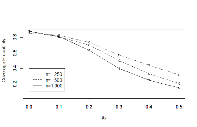
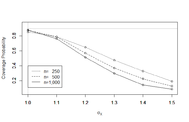
Figure 1. Simulated uniform coverage probabilities for alternative specifications of $f_{X}$ by estimated confidence bands in $I=[-2,2]$ under the standard normal random variable $X$ and an independent Laplace random vector $(\varepsilon^{(1)},\varepsilon^{(2)})$. For the top graph, the list of alternative specifications are given by $f_{X,\mu_{X}}(x)=(2\pi)^{-1/2}e^{-(x-\mu_{X})^{2}/2}$ for $\mu_{X}\in\{0.0,0.1,0.2,0.3,0.4,0.5\}$. For the bottom graph, the list of alternative specifications are given by $f_{X,\sigma_{X}}(x)=(2\pi\sigma_{X}^{2})^{-1/2}e^{-x^{2}/(2\sigma_{X}^{2})}$ for $\sigma_{X}\in\{1.0,1.1,1.2,1.3,1.4,1.5\}$. The simulated probabilities are computed for the nominal coverage probability of 90% based on 2,000 Monte Carlo iterations.

6. Application to OCS Wildcat auctions

In this section, we apply our method to the Outer Continental Shelf (OCS) Auction Data (see Hendricks et al. (1987) for details), and construct a confidence band for the density of mineral rights on oil and gas on offshore lands off the coasts of Texas and Louisiana in the gulf of Mexico. We focus on “wildcat sales,” referring to sales of those oil and gas tracts whose geological or seismic characteristics are unknown to participating firms. The sales rule follows the first-price sealed-bid auction mechanism, where participating firms simultaneously submit sealed bids, and the highest bidder pays the price they submitted to receive the right for the tract. Firms who are willing to participate in sales can carry out a seismic investigation before the sales date in order to estimate the value of mineral rights. The ex ante value $Y^{(1)}$ (in the logarithm of US dollars per acre) obtained by firm 1 through its investigation of the tract is treated as a measure of the ex post value $X$ (also known as the common component, in the logarithm of US dollars per acre) with an assessment error $\varepsilon^{(1)}$ (also known as the private component), i.e., $Y^{(1)}=X+\varepsilon^{(1)}$. Collecting the ex ante values $(Y^{(1)},Y^{(2)})$ for pairs of firms across various wildcat auctions, we can obtain data necessary to construct a uniform confidence band for the density $f_{X}$ of ex post mineral right values under our assumptions.

For this setup and for this data set, Li et al. (2000) apply the method of Li and Vuong (1998) to nonparametrically estimate $f_{X}$, but they do not obtain a confidence band. In their analysis, firms’ ex ante values $(Y^{(1)},Y^{(2)})$ are first recovered from bid data through a widely used method in economics which is based on an equilibrium restriction (Bayesian Nash equilibrium) for the first-price sealed-bid auction mechanism – see our supplementary material. In this paper, we directly take these ex ante values $(Y^{(1)},Y^{(2)})$ as the data to be used as an input for our analysis. The sample consists of 169 tracts with 2 firms in each tract. We next construct our auxiliary data $(Y,\eta)$ following Example 1.

We continue to use the same kernel function and the same bandwidth selection rule as those ones used for simulation studies in Section 5. Confidence bands for $f_{X}$ are constructed using 25,000 multiplier bootstrap replications. Figure 2 (A) shows the obtained 90% and 95% confidence bands in light gray and dark gray, respectively. The black curve draws our nonparametric estimate of $f_{X}$, and runs at the center of the bands. Our nonparametric estimate, our confidence bands, and the nonparametric estimate obtained by Li et al. (2000) – shown in their Figure 4 – are all similar to each other, and share the same qualitative characteristics. First, unlike the bimodal density of the private values $(Y^{(1)},Y^{(2)})$ (see Figure 5 in the supplementary material), the density of the common value $X$ is suggested to be single-peaked in all the results of our analysis and that of Li et al. (2000). Second, as Li et al. (2000) also emphasized, the small bump in the estimated density $f_{X}$ around $x=6$ is common in all the results. Furthermore, our confidence bands do not include zero at this locality, $x=6$. This result can be viewed as a statistical evidence in support of a significant presence of such a bump pointed out by Li et al. (2000). A more global look into the graph suggests that the 95% confidence band is bounded away from zero on the interval $[3.90,6.32]$. In other words, we can conclude that the ex post value of mineral rights in the US dollars per acre is supported on a superset of the interval $[\exp(3.90),\exp(6.32)]\approx[49,555]$, if we consider a set of density functions contained in the 95% confidence band.

(A) Unknown Error Distribution	(B) Laplace Error Distribution

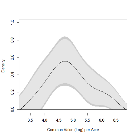
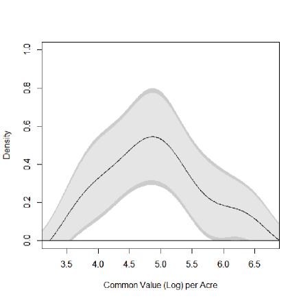
Figure 2. 90% and 95% confidence bands for $f_{X}$ marked in light gray and dark gray, respectively. The black curve in the middle indicates our deconvolution kernel density estimate of $f_{X}$.

Finally, we show an empirical result that we would obtain under the assumption that the distribution of $\varepsilon$ were known as in the previous literature. Specifically, for this exercise, we assume that $\varepsilon$ follows $\text{Laplace}\,(0,\sqrt{\sigma_{\varepsilon}^{2}/2})$, where $\sigma_{\varepsilon}^{2}=0.168$ – this number is the sample variance of $\eta_{j}$. Figure 2 (B) shows the result. There are some notable differences from Figure 2 (A). Most importantly, the 95% confidence band now contains zero around the locality, $x=6$, of the aforementioned bump in the estimated density of $X$. The contrast between Figure 2 (A) and (B) shows that there can be non-trivial differences in statistical implications of confidence bands between the case of assuming known error distribution and the case of assuming unknown error distribution.

7. Application to panel data

Example 1 demonstrates that the availability of repeated measurements with a symmetric error distribution satisfy our data requirement. A particular example of this case is the additive panel data model with fixed effects as in Horowitz and Markatou (1996):

$$Y_{j,t}=W_{j,t}^{\prime}\theta_{0}+U_{j}+V_{j,t},\quad j=1,\dots,n;t=1,2,$$

where $Y_{j,t}$ is a scalar outcome variable, $W_{j,t}$ is a $d$-dimensional vector of regressors, $\theta_{0}\in\mathbb{R}^{d}$ is the slope parameter, $U_{j}$ is an unobservable individual-specific effect, and $V_{j,t}$ is an error term. Inference on the density function of unobservables in this sort of panel data models is of interest in empirical research (e.g., Bohnomme and Robin, 2010; Bonhomme and Sauder, 2011). Horowitz and Markatou (1996) or other related panel data papers do not provide asymptotic distribution results for the density function of unobservables to our knowledge. Our method applies to inference on the density of $U_{j}$.

7.1. Methodology for panel data

We assume that

$$\begin{cases}\text{1) $\{(Y_{j,1},Y_{j,2},W_{j,1},W_{j,2},U_{j},V_{j,1},V_{j,2})\}_{j=1}^{\infty}$ are i.i.d.};\\ \text{2) $(V_{j,1},V_{j,2})$ is independent of $(W_{j,1},W_{j,2},U_{j})$};\\ \text{3) the conditional distribution of $V_{j,2}$ given $V_{j,1}$ is symmetric}.\end{cases}$$ (13)

Independence between $(V_{j,1},V_{j,2})$ and $(W_{j,1},W_{j,2})$ can be removed at the expense of more complicated regularity conditions, but we assume the independence assumption for the simplicity of exposition; see Remark 12 ahead. Horowitz and Markatou (1996) assume that $V_{j,1}$ and $V_{j,2}$ are i.i.d. and the common distribution is symmetric (see their Condition A.1); in contrast, we do not assume that $V_{j,1}$ and $V_{j,2}$ are i.i.d., nor did we assume symmetry of both distributions of $V_{j,1}$ and $V_{j,2}$. Now, consider the following transformations:

$$\begin{cases}Y_{j}^{\dagger}=(Y_{j,1}+Y_{j,2})/2-\theta_{0}^{\prime}(W_{j,1}+W_{j,2})/2,\\ \varepsilon_{j}=V_{j,1}+V_{j,2})/2,\\ \eta_{j}=(V_{j,1}-V_{j,2})/2=(Y_{j,1}-Y_{j,2})/2-\theta_{0}^{\prime}(W_{j,1}-W_{j,2})/2.\end{cases}$$

Observe that

$$Y_{j}^{\dagger}=U_{j}+\varepsilon_{j},\quad\eta_{j}\stackrel{{\scriptstyle d}}{{=}}\varepsilon_{j}.$$

We assume that the densities of $U_{j}$ and $\varepsilon_{j}$ exist and are denoted by $f_{U}$ and $f_{\varepsilon}$, respectively. The density of $Y_{j}^{\dagger}$ is given by

$$f_{Y^{\dagger}}(u)=(f_{U}*f_{\varepsilon})(u)=\int_{\mathbb{R}}f_{U}(u-y)f_{\varepsilon}(y)dy.$$

Hence, estimation of the density $f_{U}$ reduces to a deconvolution problem. The difference from the original setup is that $\theta_{0}$ is unknown and has to be estimated. We assume, as in Horowitz and Markatou (1996), that there is an estimator $\widehat{\theta}$ of $\theta_{0}$ such that $\widehat{\theta}-\theta_{0}=O_{\mathrm{P}}(n^{-1/2})$, and let

$$\begin{cases}\widehat{Y}_{j}^{\dagger}=(Y_{j,1}+Y_{j,2})/2-\widehat{\theta}^{\prime}(W_{j,1}+W_{j,2})/2,\\ \widehat{\eta}_{j}=(Y_{j,1}-Y_{j,2})/2-\widehat{\theta}^{\prime}(W_{j,1}-W_{j,2})/2.\end{cases}$$

Define

$$\varphi_{Y^{\dagger}}(t)=\mathrm{E}[e^{itY_{j}^{\dagger}}],\ \varphi_{U}(t)=\mathrm{E}[e^{itU_{j}}],\ \varphi_{\varepsilon}(t)=\mathrm{E}[e^{it\varepsilon_{j}}],$$

$$\widehat{\varphi}_{Y^{\dagger}}^{*}(t)=\frac{1}{n}\sum_{j=1}^{n}e^{itY_{j}^{\dagger}},\ \widehat{\varphi}_{Y^{\dagger}}(t)=\frac{1}{n}\sum_{j=1}^{n}e^{it\widehat{Y}_{j}^{\dagger}},\ \widehat{\varphi}_{\varepsilon}^{*}(t)=\frac{1}{n}\sum_{j=1}^{n}e^{it\eta_{j}},\ \widehat{\varphi}_{\varepsilon}(t)=\frac{1}{n}\sum_{j=1}^{n}e^{it\widehat{\eta}_{j}}.$$

Let $K:\mathbb{R}\to\mathbb{R}$ be a kernel function such that its Fourier transform $\varphi_{K}$ is supported in $[-1,1]$. The deconvolution kernel density estimator of $f_{U}$ is given by

$$\widehat{f}_{U}(u)=\frac{1}{2\pi}\int_{\mathbb{R}}e^{-itu}\widehat{\varphi}_{Y^{\dagger}}(t)\frac{\varphi_{K}(th_{n})}{\widehat{\varphi}_{\varepsilon}(t)}dt=\frac{1}{nh_{n}}\sum_{j=1}^{n}\widehat{K}_{n}((u-\widehat{Y}_{j}^{\dagger})/h_{n}),$$

where $h_{n}$ is a sequence of bandwidths tending to $0$ as $n\to\infty$, and

$$\widehat{K}_{n}(u)=\frac{1}{2\pi}\int_{\mathbb{R}}e^{-itu}\frac{\varphi_{K}(t)}{\widehat{\varphi}_{\varepsilon}(t/h_{n})}dt.$$

The rest of the procedure is the same as in Section 3. Let $\xi_{1},\dots,\xi_{n}$ be independent standard normal variables independent of the data $\mathcal{D}_{n}=\{(Y_{j,1},Y_{j,2},W_{j,1},W_{j,2})\}_{j=1}^{n}$, and consider the multiplier process

$$\widehat{Z}_{n}^{\xi}(u)=\frac{1}{\widehat{\sigma}_{n}(u)\sqrt{n}}\sum_{j=1}^{n}\xi_{j}\left\{\widehat{K}_{n}((u-\widehat{Y}^{\dagger}_{j})/h_{n})-n^{-1}{\textstyle\sum}_{j^{\prime}=1}^{n}\widehat{K}_{n}((u-\widehat{Y}^{\dagger}_{j^{\prime}})/h_{n})\right\},\ u\in I,$$

where $I\subset\mathbb{R}$ is a compact interval on which we would like to make inference on $f_{U}$, and

$$\widehat{\sigma}_{n}^{2}(u)=\frac{1}{n}\sum_{j=1}^{n}\widehat{K}_{n}^{2}((u-\widehat{Y}_{j}^{\dagger})/h_{n})-\left(\frac{1}{n}\sum_{j=1}^{n}\widehat{K}_{n}((u-\widehat{Y}_{j}^{\dagger})/h_{n})\right)^{2},\ u\in I.$$

Now, for a given $\tau\in(0,1)$, let

$$\widehat{c}_{n}(1-\tau)=\text{conditional $(1-\tau)$-quantile of $\|\widehat{Z}_{n}^{\xi}\|_{I}$ given $\mathcal{D}_{n}$},$$

and consider the confidence band

$$\widehat{\mathcal{C}}_{n}(u)=\left[\widehat{f}_{U}(u)\pm\frac{\widehat{\sigma}_{n}(u)}{\sqrt{n}h_{n}}\widehat{c}_{n}(1-\tau)\right],\ u\in I.$$ (14)

We make the following assumption for the validity of the confidence band (14).

Assumption 7.

In addition to the baseline condition (13), we assume the following conditions. (i) The function $|\varphi_{U}|$ is integrable on $\mathbb{R}$. (ii) $f_{U}\in\Sigma(\beta,B)$ for some $\beta>1/2$ and $B>0$. Let $k$ denote the integer such that $k<\beta\leq\beta+1$. (iii) Let $K:\mathbb{R}\to\mathbb{R}$ be a kernel function such that its Fourier transform $\varphi_{K}$ is supported in $[-1,1]$ and Condition (9) is satisfied. (iv) The error characteristic function $\varphi_{\varepsilon}$ is continuously differentiable and does not vanish on $\mathbb{R}$, and there exist constants $\alpha>1/2$ and $C_{1}>1$ such that $C_{1}^{-1}|t|^{-\alpha}\leq|\varphi_{\varepsilon}(t)|\leq C_{1}|t|^{-\alpha}$ and $|\varphi_{\varepsilon}^{\prime}(t)|\leq C_{1}|t|^{-\alpha-1}$ for all $|t|\geq 1$. (v) For some $p>0$, $\mathrm{E}[|\varepsilon_{1}|^{p}]<\infty$ and $\mathrm{E}[(1+|Y_{1}^{\dagger}|^{p})(\|W_{1,1}\|^{2}+\|W_{1,2}\|^{2})]<\infty$. (vi) Let $\widehat{\theta}$ be an estimator for $\theta_{0}$ such that $\widehat{\theta}-\theta_{0}=O_{\mathrm{P}}(n^{-1/2})$. (vii) Let $I$ be a compact interval in $\mathbb{R}$ such that $f_{Y^{\dagger}}(u)>0$ for all $u\in I$. (viii)

$$\frac{\log h_{n}^{-1}}{nh_{n}^{5}}\bigvee\frac{(\log h_{n}^{-1})^{2}}{nh_{n}^{2\alpha+2}}\bigvee h_{n}^{\alpha+\beta}\sqrt{nh_{n}\log h_{n}^{-1}}\to 0.$$ (15)

Furthermore, for $W_{1,t}=(W_{1,t,1},\dots,W_{1,t,d})^{\prime}$,

$$\int_{-h_{n}^{-1}}^{h_{n}^{-1}}|s\mathrm{E}[e^{isU_{1}}W_{1,t,\ell}]|ds=o\{h_{n}^{-\alpha-1/2}(\log h_{n}^{-1})^{-1/2}\},\ t=1,2;\ell=1,\dots,d.$$ (16)

These conditions ensure the asymptotic validity of the confidence band (14).

Theorem 3.

Under Assumption 7, we have that $\mathrm{P}\{f_{U}(u)\in\widehat{\mathcal{C}}_{n}(u)\ \forall u\in I\}\to 1-\tau$ as $n\to\infty$. Furthermore, the supremum width of the band $\widehat{\mathcal{C}}_{n}$ is $O_{\mathrm{P}}\{h_{n}^{-\alpha}(nh_{n})^{-1/2}\sqrt{\log h_{n}^{-1}}\}$.

Remark 11 (Discussions on Assumption 7).

These conditions are mostly adapted from the conditions given in Section 4 with $m=n$. We assume here that $\alpha>1/2$ for a technical reason to bound the impact of the estimation error in $\widehat{\theta}$ on $\widehat{f}_{U}$. Condition (15) restricts $(\alpha,\beta)$ so that $\alpha+\beta>2$, which we believe is a mild restriction. Condition (16) is another technical condition to deal with the impact of the estimation error in $\widehat{\theta}$. Condition (16) is not restrictive; in general, $|\mathrm{E}[e^{isU_{1}}W_{1,t,\ell}]|\leq\mathrm{E}[|W_{1,t,\ell}|]<\infty$, so that the left hand side on (16) is at most $O(h_{n}^{-2})$ and hence Condition (16) is satisfied as long as $\alpha>3/2$. However, Condition (16) can be satisfied without such restrictions on $\alpha$. In many cases, $|\mathrm{E}[e^{isU_{1}}W_{1,t,\ell}]|$ decays to zero as $|s|\to\infty$, which is the case if, e.g., $U_{1}$ and $W_{1,t,\ell}$ have a joint density, or $W_{1,t,\ell}$ is finitely discrete and the conditional distribution of $U_{1}$ given $W_{1,t,\ell}$ is absolutely continuous. So, if $|\mathrm{E}[e^{isU_{1}}W_{1,t,\ell}]|=O(|s|^{-\gamma})$ as $|s|\to\infty$ for some $\gamma>0$, then the left hand side on (16) is

$$\begin{cases}O(h_{n}^{\gamma-2})&\text{if}\ \gamma<2\\ O(\log h_{n}^{-1})&\text{if}\ \gamma=2\\ O(1)&\text{if}\ \gamma>2\end{cases}$$

and hence Condition (16) is satisfied as long as $\gamma>3/2-\alpha$.

Remark 12 (Independence between $(V_{j,1},V_{j,2})$ and $(W_{j,1},W_{j,2})$).

Condition (13) assumes that $(V_{j,1},V_{j,2})$ and $(U_{j},W_{j,1},W_{j,2})$ are independent. Independence between $(V_{j,1},V_{j,2})$ and $(W_{j,1},W_{j,2})$ can be removed at the cost of more complicated regularity conditions. In the proof of Theorem 3, this independence assumption is used to deduce that

$$\mathrm{E}[e^{itY_{1}^{\dagger}}W_{1,\ell}^{+}]=\varphi_{\varepsilon}(t)\mathrm{E}[e^{itU_{1}}W_{1,\ell}^{+}],\ \mathrm{E}[e^{it\eta_{1}}W_{1,\ell}^{-}]=\varphi_{\varepsilon}(t)\mathrm{E}[W_{1,\ell}^{-}],$$ (17)

where $W_{1,\ell}^{+}=(W_{1,1,\ell}+W_{1,2,\ell})/2$ and $W_{1,\ell}^{-}=(W_{1,1,\ell}-W_{1,2,\ell})/2$ for $\ell=1,\dots,d$. Now, without requiring independence between $(V_{j,1},V_{j,2})$ and $(W_{j,1},W_{j,2})$ (thereby (17) need not hold), the conclusion of Theorem 3 remains true if $\left|\frac{\mathrm{E}[e^{it\eta_{1}}W_{1,\ell}^{-}]}{\varphi_{\varepsilon}(t)}\right|$ is bounded in $t\in\mathbb{R}$, and instead of (16),

$$\int_{-h_{n}^{-1}}^{h_{n}^{-1}}\left|\frac{t\mathrm{E}[e^{itY_{1}^{\dagger}}W_{1,\ell}^{+}]}{\varphi_{\varepsilon}(t)}\right|dt=o\{h_{n}^{-\alpha-1/2}(\log h_{n}^{-1})^{-1/2}\}$$

holds for $\ell=1,\dots,d$.

7.2. Empirical illustration with panel data

Levinsohn and Petrin (2003) analyze Chilean industries for the period of 1979–1986. Following up with their studies, we analyze the distribution of the total factor productivity across firms by applying the method introduced in the previous subsection to the data set of Levinsohn and Petrin. We focus on the food industry, which is the largest industry in Chile among those studied by Levinsohn and Petrin. The data set is an unbalanced panel of $t=8$ years. The sample sizes are $n=709$ firms between 1979–1980, $n=751$ firms between 1980–1981, $n=721$ firms between 1981–1982, $n=691$ firms between 1982–1983, $n=639$ firms between 1984–1985, and $n=618$ firms between 1985–1986.

Let $Y_{j,t}$ denote the logarithm of output produced by firm $j$ in year $t$. The output is produced by using unskilled labor inputs denoted in logarithm by $W^{l^{u}}_{j,t}$, skilled labor inputs denoted in logarithm by $W^{l^{s}}_{j,t}$, capital inputs denoted in logarithm by $W^{k}_{j,t}$, material inputs denoted in logarithm by $W^{m}_{j,t}$, electricity inputs denoted in logarithm by $W^{e}_{j,t}$, and fuel inputs denoted in logarithm by $W^{u}_{j,t}$. In addition, we include two time-period dummies, $W^{d^{1}}_{j,t}$ and $W^{d^{2}}_{j,t}$ for 1982–1983 and 1984–1986, respectively, following the time periods defined by Levinsohn and Petrin (2003). Gross-output production function in logs is written as

$$Y_{j,t}=W_{j,t}^{\prime}\theta_{0}+\omega_{j,t}+\eta_{j,t}$$

where $W_{j,t}=(W^{l^{u}}_{j,t},W^{l^{s}}_{j,t},W^{k}_{j,t},W^{m}_{j,t},W^{e}_{j,t},W^{u}_{j,t},W^{d^{1}}_{j,t},W^{d^{2}}_{j,t})$, $\theta_{0}=(\theta_{lu},\theta_{ls},\theta_{k},\theta_{m},\theta_{e},\theta_{u},\theta_{d^{1}},\theta_{d^{2}})^{\prime}$, $\omega_{j,t}$ denotes the productivity, and $\eta_{j,t}$ denotes an idiosyncratic shock.

Rational firms accumulate state variables and make static input choices endogenously in response to the current and past productivity levels, and thus $W_{j,t}$ is not statistically independent of $\omega_{j,t}$. Under the presence of this endogeneity, various approaches (Olley and Pakes, 1996; Levinsohn and Petrin, 2003; Ackerberg et al., 2006; Wooldridge, 2009) are developed for identification and consistent estimation of the production function parameters $\theta_{0}$. We use the GMM criterion of Wooldridge (2009) to estimate these parameters with the third degree polynomial control of $\omega_{j,t}$ and with $W^{m}_{j,t}$ as a proxy following Levinsohn and Petrin by pooling all the observations in the data. Let the estimate be denoted by $\widehat{\theta}$.

Focusing on any pair of two adjacent time periods, we can rewrite the gross-output production function as a panel data model with fixed effects as follows.

$$Y_{j,t}=W_{j,t}^{\prime}\theta_{0}+U_{j}+V_{j,t},\qquad j=1,...,n;t=1,2,$$

where $U_{j}=\omega_{j,1}$, $V_{j,1}=\eta_{j,1}$ and $V_{j,2}=\omega_{j,2}-\omega_{j,1}+\eta_{j,2}$. Following the method proposed in the previous subsection, we construct the auxiliary variables

$$Y_{j}^{\dagger} =(Y_{j,1}+Y_{j,2})/2-\theta_{0}^{\prime}(W_{j,1}+W_{j,2})/2=U_{j}+(V_{j,1}+V_{j,2})/2$$

$$\eta_{j} =(Y_{j,1}-Y_{j,2})/2-\theta_{0}^{\prime}(W_{j,1}-W_{j,2})/2=(V_{j,1}-V_{j,2})/2$$

The independence condition between $U_{j}$ and $(V_{j,1},V_{j,2})$ is satisfied if

1. the productivity $\omega_{j,1}$ and the idiosyncratic shocks $(\eta_{j,1},\eta_{j,2})$ are independent; and

2. the productivity $\omega_{j,1}$ and the productivity innovation $\omega_{j,2}-\omega_{j,1}$ are independet.

These conditions are assumed in the aforementioned production function papers, and we thus maintain this primitive assumption in order to satisfy our high-level independence condition. We substitute the above estimate $\widehat{\theta}$ for $\theta_{0}$ and use

$$\widehat{Y}_{j}^{\dagger} =(Y_{j,1}+Y_{j,2})/2-\widehat{\theta}^{\prime}(W_{j,1}+W_{j,2})/2$$

$$\widehat{\eta}_{j} =(Y_{j,1}-Y_{j,2})/2-\widehat{\theta}^{\prime}(W_{j,1}-W_{j,2})/2$$

to apply our method.

We continue to use the same kernel function and the same bandwidth selection rule as those ones used for simulation studies in Section 5. Confidence bands for $f_{\omega_{j,t}}$ are constructed for each $t=$1979–1985 using 25,000 multiplier bootstrap replications. Figure 3 shows the 90% and 95% confidence bands as well as the estimate for $f_{\omega_{j,t}}$ for years $t=$1979–1982. Figure 4 shows the 90% and 95% confidence bands as well as the estimate for $f_{\omega_{j,t}}$ for years $t=$1982–1985. Observe that the distribution of the productivities is shifting to the right as time progresses. Furthermore, the constructed confidence bands informatively indicate the possible densities accounting for uncertainties in data sampling.

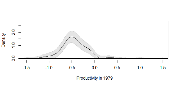
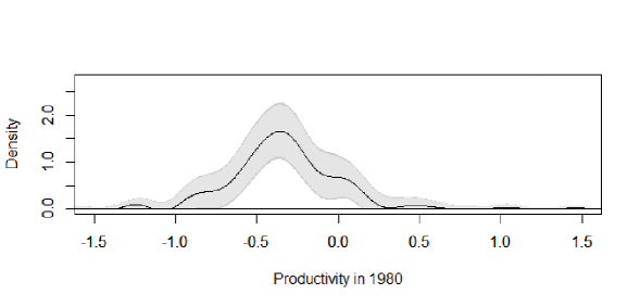
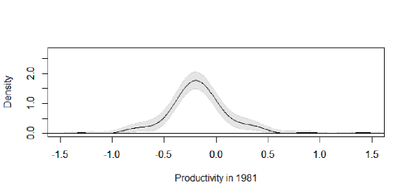
Figure 3. 90% and 95% confidence bands for $f_{\omega_{j,t}}$ marked in light gray and dark gray, respectively. The black curve in the middle indicates the deconvolution kernel density estimate.

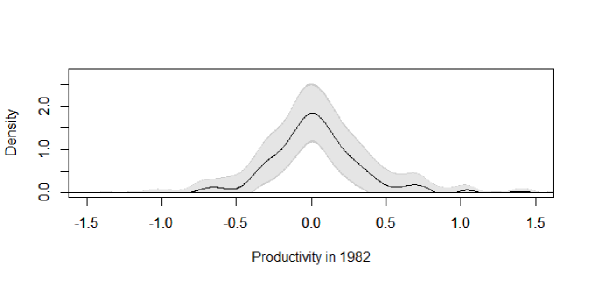
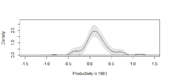
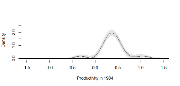
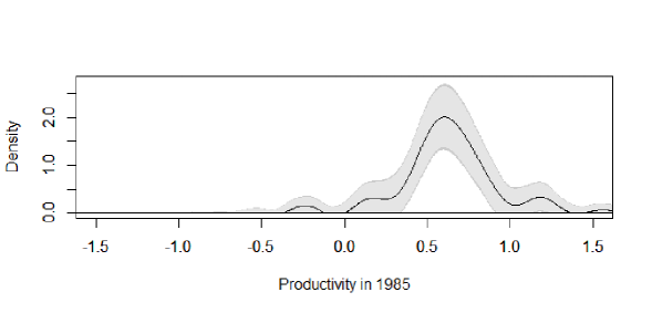
Figure 4. 90% and 95% confidence bands for $f_{\omega_{j,t}}$ marked in light gray and dark gray, respectively. The black curve in the middle indicates the deconvolution kernel density estimate.

8. Extensions to super-smooth case

In this section, we consider extensions of the results on confidence bands to the case where the error density $f_{\varepsilon}$ is super-smooth. While some notations were changed in Section 7 to accommodate panel data models, we switch back in this section to the original notations used prior to Section 7. We still keep Assumptions 1 and 5, but require a different set of assumptions on the kernel function $K$, the bandwidth $h_{n}$, and the sample size $m$ for $f_{\varepsilon}$. It turns out that from a technical reason, we require $m/n\to\infty$ in the super-smooth case, and so Example 1 is formally not covered in the super-smooth case. Still, we believe that the extensions to the super-smooth case are of some interest.

We modify Assumptions 2, 3, and 6 as follows. First, for the kernel and error characteristic functions, we assume the following conditions.

Assumption 8.

Let $K:\mathbb{R}\to\mathbb{R}$ be a kernel function such that its Fourier transform $\varphi_{K}$ is even (i.e., $\varphi_{K}(-t)=\varphi_{K}(t)$) and has support $[-1,1]$. Furthermore, there exist constants $C_{2}>0$ and $\lambda\geq 0$ such that $\varphi_{K}(1-t)=C_{2}t^{\lambda}+o(t^{\lambda})$ as $t\downarrow 0$.

Assumption 9.

The error characteristic function $\varphi_{\varepsilon}$ does not vanish on $\mathbb{R}$, and there exist constants $C_{3}>0,\gamma>1,\gamma_{0}\in\mathbb{R},\nu>0$ such that $\varphi_{\varepsilon}(t)=C_{3}(1+o(1))|t|^{\gamma_{0}}e^{-\nu|t|^{\gamma}}$ as $|t|\to\infty$.

These assumptions are adapted from van Es and Uh (2005). Assumption 9 covers cases where the error characteristic function decays exponentially fast as $|t|\to\infty$, thereby covering cases where the error density is super-smooth. However, Assumption 9 is more restrictive than standard super-smoothness conditions; e.g., it excludes the Cauchy error. This assumption is needed to derive a lower bound on $\sigma_{n}^{2}(x)$; see the following discussion.

Assumptions 8 and 9, together with the assumption that $\mathrm{E}[Y^{2}]<\infty$, ensure that the variance function $\sigma_{n}^{2}(x)=\operatorname{Var}(K_{n}((x-Y)/h_{n}))$ is expanded as

$$\sigma_{n}^{2}(x)=(1+o(1))\frac{C_{2}^{2}}{2C_{3}^{2}\pi^{2}}(\nu\gamma)^{-2\lambda-2}(\Gamma(\lambda+1))^{2}h_{n}^{2\gamma(1+\lambda)+2\gamma_{0}}e^{2\nu h_{n}^{-\gamma}}$$ (18)

as $n\to\infty$; see the proof of Theorem 1.5 in van Es and Uh (2005). It is not difficult to verify from their proof that $o(1)$ in (18) is uniform in $x\in I$ for any compact interval $I\subset\mathbb{R}$. It is worthwhile to point out that, in contrast to the ordinary smooth case, the lower bound on $\sigma_{n}^{2}(x)$ in (18) does not explicitly depend on $x$ nor $f_{Y}$. Further, Assumption 9 implies that

$$\inf_{|t|\leq h_{n}^{-1}}|\varphi_{\varepsilon}(t)|\geq C_{3}(1-o(1))h_{n}^{-\gamma_{0}}e^{-\nu h_{n}^{-\gamma}}$$ (19)

as $n\to\infty$. It turns out that (18) and (19) are the only differences to take care of when proving the analogues of Theorems 1 and 2 in the super-smooth case. Finally, we modify Assumption 6 as follows.

Assumption 10.

(a) $\frac{(\log h_{n}^{-1})^{2}}{nh_{n}^{4\gamma(1+\lambda)}}\to 0$. (b) $\frac{n\log h_{n}^{-1}}{mh_{n}^{2\gamma(1+\lambda)-2}}\bigvee\frac{e^{2\nu h{n}^{-\gamma}}(\log h_{n}^{-1})^{2}}{mh_{n}^{4\gamma(1+\lambda)-2\gamma_{0}}}\to 0$.

The requirement that $\frac{n\log h_{n}^{-1}}{mh_{n}^{2\gamma(1+\lambda)-2}}\to 0$ implies that we at least need $m/n\to\infty$. This condition is used to ensure that the effect of estimating $\varphi_{\varepsilon}$ is negligible. To be precise, in our proof, a bound on $\|\widehat{f}_{X}-\widehat{f}_{X}^{*}\|_{\mathbb{R}}$ involves a term of order $m^{-1/2}h_{n}^{\gamma_{0}}e^{\nu h_{n}^{-\gamma}}$, which has to be of smaller order than $n^{-1/2}h_{n}^{\gamma(1+\lambda)+\gamma_{0}-1}e^{\nu h_{n}^{-\gamma}}(\log h_{n}^{-1})^{-1/2}$. Technically, this problem happens because the ratio of $1/\inf_{|t|\leq h_{n}^{-1}}|\varphi_{\varepsilon}(t)|$ over $\inf_{x\in I}\sigma_{n}(x)$ is larger in the super-smooth case than that in the ordinary smooth case; the ratio is $O(h_{n}^{-\gamma(1+\lambda)})$ in the super-smooth case, while it is $O(h_{n}^{-1/2})$ in the ordinary smooth case. It is not known at the current moment whether we could relax this condition on $m$ in the super-smooth case.

In any case, these assumptions guarantee that the conclusions of Theorems 1 and 2, except for the result on the width of the band, hold true in the super-smooth case.

Theorem 4.

Suppose that Assumptions 1, 5, and 8–10 are satisfied. Let $I\subset\mathbb{R}$ be any compact interval, and suppose in addition that $\mathrm{E}[Y^{2}]<\infty$. Then the conclusions of Theorems 1 and 2 , except for the result on the width of the band, hold true.

Remark 13 (Comparisons with van Es and Gugushvili (2008)).

van Es and Gugushvili (2008) prove that, under the assumptions that $f_{\varepsilon}$ is known and satisfies Assumption 9 (of the present paper) with $\gamma=2$,

$$\frac{\sqrt{n}}{h_{n}^{2(1+\lambda)+\gamma_{0}-1}e^{\nu h_{n}^{-2}}}\|\widehat{f}_{X}^{*}(\cdot)-\mathrm{E}[\widehat{f}_{X}^{*}(\cdot)]\|_{[0,1]}\stackrel{{\scriptstyle d}}{{\to}}\frac{C_{2}}{\sqrt{2}C_{3}\pi}(2\nu)^{-\lambda-1}\Gamma(\lambda+1)V,$$

where $V$ follows the Rayleigh distribution, i.e., $V$ is a random variable having density $f_{V}(v)=ve^{-v^{2}/2}1_{[0,\infty)}(v)$ (see van Es and Gugushvili, 2008, for the precise regularity conditions). Interestingly, the limit distribution differs from Gumbel distributions.

Despite this non-standard feature, Theorem 4 shows that the multiplier bootstrap “works”, i.e., the conditional distribution of $\|\widehat{Z}_{n}^{\xi}\|_{I}$ can consistently estimate the distribution of $\|\widehat{Z}_{n}\|_{I}$ in the sense that $\sup_{z\in\mathbb{R}}|\mathrm{P}\{\|\widehat{Z}_{n}^{\xi}\|_{I}\leq z\mid\mathcal{D}_{n}\}-\mathrm{P}\{\|\widehat{Z}_{n}\|_{I}\leq z\}|\stackrel{{\scriptstyle\mathrm{P}}}{{\to}}0$. Further, Theorem 4 extends the admissible range of $\gamma$ compared with the result of van Es and Gugushvili (2008).

If $f_{X}$ belongs to a Hölder ball $\Sigma(\beta,B)$, then we have the following corollary.

Corollary 4.

Assume all the conditions of Theorem 4. Further, suppose that $f_{X}\in\Sigma(\beta,B)$ for some $\beta>0,B>0$, and that Condition (9) is satisfied for the kernel function $K$ where $k$ is the integer such that $\beta<k\leq\beta+1$. Consider the multiplier bootstrap confidence band $\widehat{\mathcal{C}}_{n}$ defined in (7). Then as $n\to\infty$, $\mathrm{P}\{f_{X}(x)\in\widehat{\mathcal{C}}_{n}(x)\ \forall x\in I\}\to 1-\tau$, provided that $h_{n}^{\beta+1-\gamma(1+\lambda)-\gamma_{0}}e^{-\nu h_{n}^{-\gamma}}\sqrt{n\log h_{n}^{-1}}\to 0$.

9. Conclusion

The previous literature on inference in deconvolution has focused on the case where the error distribution is known. In econometric applications, the assumption that the error distribution is known is unrealistic, and the present paper fills this important void. Specifically, we develop a method to construct uniform confidence bands in deconvolution when the error distribution is unknown and needs to be estimated with an auxiliary sample from the error distribution. The auxiliary sample may directly come from validation data, such as administrative data, or can be constructed from panel data with a symmetric error distribution.

We first focus on the baseline setting where the error density is ordinary smooth. The construction is based upon the “intermediate” Gaussian approximation and the Gaussian multiplier bootstrap, instead of explicit limit distributions such as Gumbel distributions. This approach allows us to prove the validity of the proposed multiplier bootstrap confidence band under mild regularity conditions. Simulation studies demonstrate that the multiplier bootstrap confidence bands perform well in the finite sample. We apply our method to the Outer Continental Shelf (OCS) Auction Data and draw confidence bands for the density of common values of mineral rights on oil and gas tracts. We also discuss an application of our main result to additive fixed-effect panel data models. As an empirical illustration of the panel analysis, we draw confidence bands for the density of the total factor productivity in the food manufacturing industry in Chile following the analysis of Levinsohn and Petrin (2003). Finally, we present extensions of the baseline theoretical results to the case of super-smooth error densities.

Throughout this paper, we suppose the availability of an auxiliary sample, an example of which is panel data with a symmetric error distribution similarly to Horowitz and Markatou (1996). The estimator of Li and Vuong (1998), on the other hand, relaxes the assumption of a symmetric error distribution. An extension of our results on the method of inference to this case is left for future research.

Appendix A Proofs

In what follows, the notation $\lesssim$ signifies that the left hand side is bounded by the right hand side up to some constant independent of $n$ and $x$.

A.1. Proof of Theorem 1

We first state the following lemmas which will be used in the proof of Theorem 1. For a class of measurable functions $\mathcal{F}$ on a measurable space $(S,\mathcal{S})$ and a probability measure $Q$ on $\mathcal{S}$, let $N(\mathcal{F},\|\cdot\|_{Q,2},\delta)$ denote the $\delta$-covering number for $\mathcal{F}$ with respect to the $L^{2}(Q)$-seminorm $\|\cdot\|_{Q,2}$; see Section 2.1 in van der Vaart and Wellner (1996) for details.

Lemma 1.

Let $K$ be a kernel function on $\mathbb{R}$ such that $\varphi_{K}$ is supported in $[-1,1]$, and suppose that $\varphi_{\varepsilon}$ does not vanish on $\mathbb{R}$. Let $r_{n}=1/\inf_{|t|\leq h_{n}^{-1}}|\varphi_{\varepsilon}(t)|$. Consider the class of functions $\mathcal{K}_{n}=\{y\mapsto K_{n}((x-y)/h_{n}):x\in\mathbb{R}\}$, where $K_{n}$ denotes the corresponding deconvolution kernel. Then there exist constants $A,v>0$ independent of $n$ such that for all $n\geq 1$,

$$\sup_{Q}N(\mathcal{K}_{n},\|\cdot\|_{Q,2},r_{n}\delta)\leq(A/\delta)^{v},\ 0<\forall\delta\leq 1,$$

where $\sup_{Q}$ is taken over all Borel probability measures $Q$ on $\mathbb{R}$.

In view of Lemma 1 in Giné and Nickl (2009) (or Proposition 3.6.12 in Giné and Nickl (2016)), Lemma 1 follows as soon as we show that $K_{n}$ has quadratic variation $\lesssim r_{n}^{2}$. Recall that a real-valued function $f$ on $\mathbb{R}$ is said to be of bounded $p$-variation for $p\in[1,\infty)$ if

$$V_{p}(f):=\sup\Bigg{\{}\sum_{\ell=1}^{N}|f(x_{\ell})-f(x_{\ell-1})|^{p}:-\infty<x_{0}<\cdots<x_{N}<\infty,N=1,2,\dots\Bigg{\}}$$

is finite. A function of bounded $2$-variation is said to be of bounded quadratic variation. Now, Lemma 1 follows from the next lemma.

Lemma 2.

Assume the same conditions as in Lemma 1. Then the deconvolution kernel $K_{n}$ is of bounded quadratic variation with $V_{2}(K_{n})\lesssim r_{n}^{2}$.

Proof.

The basic idea of the proof is due to the proof of Lemma 1 in Lounici and Nickl (2011). In view of the continuous embedding of the homogeneous Besov space $\dot{B}_{2,1}^{1/2}(\mathbb{R})$ into $BV_{2}(\mathbb{R})$, the space of functions of bounded quadratic variation (Bourdaud et al., 2006, Theorem 5), it is enough to show that $\|K_{n}\|_{\dot{B}_{2,1}^{1/2}}\lesssim r_{n}$, where

$$\|f\|_{\dot{B}_{2,1}^{1/2}}=\int_{\mathbb{R}}\frac{1}{|u|^{3/2}}\left(\int_{\mathbb{R}}|f(x+u)-f(x)|^{2}dx\right)^{1/2}du.$$

Precisely speaking, for any real-valued function $f$ on $\mathbb{R}$ that vanishes at infinity (i.e., $\lim_{|x|\to\infty}f(x)=0$), the following bound holds: $V_{2}(f)^{1/2}\lesssim\|f\|_{B_{2,1}^{1/2}}$ up to a constant independent of $f$. Observe that $K_{n}$ vanishes at infinity by the Riemann-Lebesgue lemma. Let $\psi_{n}(t)=\varphi_{K}(t)/\varphi_{\varepsilon}(t/h_{n})$, and observe that, using Plancherel’s theorem,

$$\int_{\mathbb{R}}|K_{n}(x+u)-K_{n}(x)|^{2}dx=\frac{1}{2\pi}\int_{\mathbb{R}}|e^{-itu}-1|^{2}|\psi_{n}(t)|^{2}dt=\frac{1}{\pi}\int_{\mathbb{R}}(1-\cos(tu))|\psi_{n}(t)|^{2}dt.$$

Using the inequality $1-\cos(tu)\leq\min\{2,(tu)^{2}/2\}$, we conclude that

$$\|K_{n}\|_{\dot{B}_{2,1}^{1/2}} \lesssim\left(\int_{\mathbb{R}}t^{2}|\psi_{n}(t)|^{2}dt\right)^{1/2}\int_{[-1,1]}\frac{1}{|u|^{1/2}}du+\left(\int_{\mathbb{R}}|\psi_{n}(t)|^{2}dt\right)^{1/2}\int_{[-1,1]^{c}}\frac{1}{|u|^{3/2}}du$$

$$\lesssim r_{n}.$$

This completes the proof. ∎

Remark 14.

Lemma 1 generalizes a part of Lemma 5.3.5 in Giné and Nickl (2016) that focuses on the case where the bandwidth $h_{n}$ takes values in $\{2^{-k}:k=1,2,\dots\}$. The proof of Lemma 1 appears to be simpler than that of Lemma 5.3.5 in Giné and Nickl (2016) (but note that Lemma 5.3.5 in Giné and Nickl (2016) also covers wavelet kernels).

Lemma 3.

Assumptions 1–4 imply that, for sufficiently large $n$, $\inf_{x\in I}\sigma_{n}^{2}(x)\gtrsim h_{n}^{-2\alpha+1}$.

Proof.

The proof is inspired by Fan (1991b). The difficulty here is that $K_{n}$ has unbounded support (since its Fourier transform $\frac{\varphi_{K}}{\varphi_{\varepsilon}(\cdot/h_{n})}$ is compactly supported) and depends intrinsically on $n$. Observe first that $\|K_{n}\|_{\mathbb{R}}\lesssim h_{n}^{-\alpha}$. Second, integration by parts yields that

$$K_{n}(x)=\frac{1}{2\pi ix}\int_{\mathbb{R}}e^{-itx}\left\{\frac{\varphi_{K}(t)}{\varphi_{\varepsilon}(t/h_{n})}\right\}^{\prime}dt=\frac{1}{2\pi ix}\int_{\mathbb{R}}e^{-itx}\left\{\frac{\varphi_{K}^{\prime}(t)}{\varphi_{\varepsilon}(t/h_{n})}-\frac{\varphi_{K}(t)\varphi_{\varepsilon}^{\prime}(t/h_{n})}{h_{n}\varphi^{2}_{\varepsilon}(t/h_{n})}\right\}dt.$$

It is not difficult to verify that

$$\int_{\mathbb{R}}\left|\frac{\varphi_{K}^{\prime}(t)}{\varphi_{\varepsilon}(t/h_{n})}\right|dt\lesssim h_{n}^{-\alpha}.$$

Splitting the integral into $|t/h_{n}|\leq 1$ and $|t/h_{n}|>1$, we also see that

$$\left\{\int_{|t/h_{n}|\leq 1}+\int_{|t/h_{n}|>1}\right\}\left|\frac{\varphi_{K}(t)\varphi_{\varepsilon}^{\prime}(t/h_{n})}{h_{n}\varphi^{2}_{\varepsilon}(t/h_{n})}\right|dt\lesssim 1+h_{n}^{-\alpha}\int_{\mathbb{R}}|t|^{\alpha-1}|\varphi_{K}(t)|dt,$$

which is $\lesssim h_{n}^{-\alpha}$. This yields that $h_{n}^{2\alpha}K_{n}^{2}(x)\lesssim 1/x^{2}$, and so $h_{n}^{2\alpha}K_{n}^{2}(x)\lesssim\min\{1,1/x^{2}\}$.

Now, observe that

$$|\mathrm{E}[K_{n}((x-Y)/h_{n})]| =h_{n}\left|\int_{\mathbb{R}}K(y)f_{X}(x-h_{n}y)dy\right|$$

$$\leq h_{n}\|f_{X}\|_{\mathbb{R}}\int_{\mathbb{R}}|K(y)|dy=O(h_{n}),\ \text{and}$$

$$\mathrm{E}[K_{n}^{2}((x-Y)/h_{n})] =h_{n}\int_{\mathbb{R}}K_{n}^{2}(y)f_{Y}(x-h_{n}y)dy.$$

So, it is enough to prove that

$$\inf_{x\in I}\int_{\mathbb{R}}K_{n}^{2}(y)f_{Y}(x-h_{n}y)dy\gtrsim(1-o(1))h_{n}^{-2\alpha}.$$

To this end, since

$$\int_{\mathbb{R}}K_{n}^{2}(y)dy=\frac{1}{2\pi}\int_{\mathbb{R}}\frac{|\varphi_{K}(t)|^{2}}{|\varphi_{\varepsilon}(t/h_{n})|^{2}}dt\gtrsim h_{n}^{-2\alpha},$$

by Plancherel’s theorem (we have used that $|\varphi_{\varepsilon}(t)|\leq C_{1}|t|^{-\alpha}$ for $|t|\geq 1$ to deduce the last inequality), it is enough to prove that as $n\to\infty$,

$$\sup_{x\in I}\left|h_{n}^{2\alpha}\int_{\mathbb{R}}K_{n}^{2}(y)\{f_{Y}(x-h_{n}y)-f_{Y}(x)\}dy\right|\to 0.$$

Since $f_{Y}$ is continuous and $I$ is compact, for any $\rho>0$, there exists $\delta>0$ such that $\sup_{x\in I}|f_{Y}(x-y)-f_{Y}(x)|\leq\rho$ whenever $|y|\leq\delta$. So,

$$\sup_{x\in I}h_{n}^{2\alpha}\int_{\mathbb{R}}K_{n}^{2}(y)|f_{Y}(x-h_{n}y)-f_{Y}(x)|dy$$

$$\quad\lesssim\rho\int_{|y|\leq\delta/h_{n}}\min\{1,1/y^{2}\}dy+2\|f_{Y}\|_{\mathbb{R}}\int_{|y|>\delta/h_{n}}y^{-2}dy\lesssim\rho+o(1),$$

which yields the desired conclusion. ∎

Proof of Theorem 1.

We divide the proof into three steps.

Step 1. (Gaussian approximation to $Z_{n}^{*}$). Recall the empirical process $Z_{n}^{*}(x),x\in I$ defined as

$$Z_{n}^{*}(x) =\frac{\sqrt{n}h_{n}\{\widehat{f}_{X}^{*}(x)-\mathrm{E}[\widehat{f}_{X}^{*}(x)]\}}{\sigma_{n}(x)}$$

$$=\frac{1}{\sigma_{n}(x)\sqrt{n}}\sum_{j=1}^{n}\{K_{n}((x-Y_{j})/h_{n})-\mathrm{E}[K_{n}((x-Y)/h_{n})]\},\ x\in I.$$

Consider the class of functions

$$\mathcal{G}_{n}=\left\{\frac{1}{\sigma_{n}(x)}\{K_{n}((x-\cdot)/h_{n})-\operatorname{E}[K_{n}((x-Y)/h_{n})]\}:x\in I\right\},$$

together with the empirical process indexed by $\mathcal{G}_{n}$ defined as

$$\mathcal{G}_{n}\ni g\mapsto\nu_{n}(g)=\frac{1}{\sqrt{n}}\sum_{j=1}^{n}g(Y_{j}).$$

Observe that $\|Z_{n}^{*}\|_{I}=\|\nu_{n}\|_{\mathcal{G}_{n}}$. We apply Corollary 2.2 in Chernozhukov et al. (2014a) to $\|\nu_{n}\|_{\mathcal{G}_{n}}$. First, since the set $\{1/\sigma_{n}(x):x\in I\}$ is bounded with $\|1/\sigma_{n}\|_{I}\lesssim h_{n}^{\alpha-1/2}$, in view of Lemma 1 of the present paper and Corollary A.1 in Chernozhukov et al. (2014a), there exist constants $A^{\prime},v^{\prime}>0$ independent of $n$ such that

$$\sup_{Q}N(\mathcal{G}_{n},\|\cdot\|_{Q,2},\delta/\sqrt{h_{n}})\leq(A^{\prime}/\delta)^{v^{\prime}},\ 0<\forall\delta\leq 1,$$ (20)

which ensures the existence a tight Gaussian random variable $G_{n}$ in $\ell^{\infty}(\mathcal{G}_{n})$ with mean zero and the same covariance function as $\nu_{n}$ (cf. Chernozhukov et al., 2014a, Lemma 2.1). Since $\|K_{n}((x-\cdot)/h_{n})/\sigma_{n}(x)\|_{\mathbb{R}}\lesssim 1/\sqrt{h_{n}}$ and $\operatorname{Var}(K_{n}((x-Y)/h_{n})/\sigma_{n}(x))=1$, application of Corollary 2.2 in Chernozhukov et al. (2014a) with $q=\infty,b\lesssim 1/\sqrt{h_{n}},\sigma=1,A\lesssim 1,v\lesssim 1$, and $\gamma=1/\log n$, yields that there exists a sequence of random variables $W_{n}$ with $W_{n}\stackrel{{\scriptstyle d}}{{=}}\|G_{n}\|_{\mathcal{G}_{n}}$ (where the notation $\stackrel{{\scriptstyle d}}{{=}}$ signifies equality in distribution) and such that

$$\left|\|\nu_{n}\|_{\mathcal{G}_{n}}-W_{n}\right|=O_{\mathrm{P}}\{(\log n)/(nh_{n})^{1/6}\},$$ (21)

where the left hand side is equal to $|\|Z_{n}^{*}\|_{I}-W_{n}|$.

Next, for $f_{n,x}(\cdot)=\{K_{n}((x-\cdot)/h_{n})-\operatorname{E}[K_{n}((x-Y)/h_{n})]\}/\sigma_{n}(x)$, define

$$Z_{n}^{G}(x)=G_{n}\left(f_{n,x}\right),\ x\in I,$$

and observe that $Z_{n}^{G}$ is a tight Gaussian random variable in $\ell^{\infty}(I)$ with mean zero and the same covariance function as $Z_{n}^{*}$, and such that $\|Z_{n}^{G}\|_{I}=\|G_{n}\|_{\mathcal{G}_{n}}\stackrel{{\scriptstyle d}}{{=}}W_{n}$. It is worth noting that deducing from (21) a bound on

$$\sup_{z\in\mathbb{R}}\left|\mathrm{P}\{\|Z^{*}_{n}\|_{I}\leq z\}-\mathrm{P}\{\|Z_{n}^{G}\|_{I}\leq z\}\right|$$

is a non-trivial step, since the distribution of the approximating Gaussian process $Z_{n}^{G}$ changes with $n$. To this end, we will use the anti-concentration inequality for the supremum of a Gaussian process, which yields that

$$\sup_{z\in\mathbb{R};\Delta>0}\frac{\mathrm{P}\{z-\Delta\leq\|Z_{n}^{G}\|_{I}\leq z+\Delta\}}{\Delta}\lesssim\mathrm{E}[\|Z_{n}^{G}\|_{I}].$$ (22)

See Corollary 2.1 in Chernozhukov et al. (2014b) (see also Theorem 3 in Chernozhukov et al. (2015)). To apply this inequality, we shall bound $\mathrm{E}[\|Z_{n}^{G}\|_{I}]=\mathrm{E}[\|G_{n}\|_{\mathcal{G}_{n}}]$, but given the covering number bound (20) and $\operatorname{Var}(K_{n}((x-Y)/h_{n})/\sigma_{n}(x))=1$, Dudley’s entropy integral bound (cf. van der Vaart and Wellner, 1996, Corollary 2.2.8) yields that

$$\operatorname{E}[\|G_{n}\|_{\mathcal{G}_{n}}]\lesssim\int_{0}^{1}\sqrt{1+\log(1/(\delta\sqrt{h}_{n}))}d\delta\lesssim\sqrt{\log h_{n}^{-1}}.$$

Now, combining (21) with the anti-concentration inequality (22), we conclude that

$$\sup_{z\in\mathbb{R}}\left|\mathrm{P}\{\|Z^{*}_{n}\|_{I}\leq z\}-\mathrm{P}\{\|Z_{n}^{G}\|_{I}\leq z\}\right|\to 0,$$

provided that $\frac{(\log n)\sqrt{\log h_{n}^{-1}}}{(nh_{n})^{1/6}}\to 0$, which is satisfied under our assumption.

Step 2. (Gaussian approximation to the intermediate process). Define the intermediate process

$$\widetilde{Z}_{n}(x)=\frac{\sqrt{n}h_{n}\{\widehat{f}_{X}(x)-\mathrm{E}[\widehat{f}_{X}^{*}(x)]\}}{\sigma_{n}(x)},\ x\in I,$$

where the difference from $\widehat{Z}_{n}(x)$ is that $\widehat{\sigma}_{n}(x)$ is replaced by $\sigma_{n}(x)$. In this step, we wish to prove that

$$\sup_{z\in\mathbb{R}}|\mathrm{P}\{\|\widetilde{Z}_{n}\|_{I}\leq z\}-\mathrm{P}\{\|Z_{n}^{G}\|_{I}\leq z\}|\to 0,$$ (23)

where $Z_{n}^{G}$ is given in the previous step.

Since $\varphi_{\varepsilon}$ does not vanish on $\mathbb{R}$, we have that $\{\varphi_{Y}\neq 0\}=\{\varphi_{X}\neq 0\}$, so that we have

$$\widehat{f}_{X}^{*}(x) =\frac{1}{2\pi}\left\{\int_{\{\varphi_{X}\neq 0\}}e^{-itx}\varphi_{K}(th_{n})\frac{\widehat{\varphi}_{Y}(t)}{\varphi_{Y}(t)}\varphi_{X}(t)dt+\int_{\{\varphi_{X}=0\}}e^{-itx}\frac{\varphi_{K}(th_{n})}{\varphi_{\varepsilon}(t)}\widehat{\varphi}_{Y}(t)dt\right\},\ \text{and}$$

$$\widehat{f}_{X}(x) =\frac{1}{2\pi}\Bigg{\{}\int_{\{\varphi_{X}\neq 0\}}e^{-itx}\varphi_{K}(th_{n})\frac{\widehat{\varphi}_{Y}(t)}{\varphi_{Y}(t)}\frac{\varphi_{\varepsilon}(t)}{\widehat{\varphi}_{\varepsilon}(t)}\varphi_{X}(t)dt+\int_{\{\varphi_{X}=0\}}e^{-itx}\frac{\varphi_{K}(th_{n})}{\varphi_{\varepsilon}(t)}\widehat{\varphi}_{Y}(t)\frac{\varphi_{\varepsilon}(t)}{\widehat{\varphi}_{\varepsilon}(t)}dt\Bigg{\}}.$$

So, letting

$$\widetilde{f}_{X}(x)=\frac{1}{2\pi}\int_{\mathbb{R}}e^{-itx}\varphi_{K}(th_{n})\frac{\varphi_{\varepsilon}(t)}{\widehat{\varphi}_{\varepsilon}(t)}\varphi_{X}(t)dt,$$

we obtain the following decomposition:

$$\widehat{f}_{X}(x)-\widehat{f}^{*}_{X}(x)$$

$$=\left[\{\widehat{f}_{X}(x)-\widetilde{f}_{X}(x)\}-\{\widehat{f}_{X}^{*}(x)-\mathrm{E}[\widehat{f}_{X}^{*}(x)]\}\right]+\{\widetilde{f}_{X}(x)-\mathrm{E}[\widehat{f}_{X}^{*}(x)]\}$$

$$=\frac{1}{2\pi}\int_{\{\varphi_{X}\neq 0\}}e^{-itx}\varphi_{K}(th_{n})\left\{\frac{\widehat{\varphi}_{Y}(t)}{\varphi_{Y}(t)}-1\right\}\left\{\frac{\varphi_{\varepsilon}(t)}{\widehat{\varphi}_{\varepsilon}(t)}-1\right\}\varphi_{X}(t)dt$$

$$\quad+\frac{1}{2\pi}\int_{\{\varphi_{X}=0\}}e^{-itx}\frac{\varphi_{K}(th_{n})}{\varphi_{\varepsilon}(t)}\widehat{\varphi}_{Y}(t)\left\{\frac{\varphi_{\varepsilon}(t)}{\widehat{\varphi}_{\varepsilon}(t)}-1\right\}dt$$

$$\quad+\frac{1}{2\pi}\int_{\mathbb{R}}e^{-itx}\varphi_{K}(th_{n})\left\{\frac{\varphi_{\varepsilon}(t)}{\widehat{\varphi}_{\varepsilon}(t)}-1\right\}\varphi_{X}(t)dt.$$

Hence the Cauchy-Schwarz inequality yields that

$$|\widehat{f}_{X}(x)-\widehat{f}_{X}^{*}(x)|^{2} \lesssim\left\{\int_{\{\varphi_{X}\neq 0\}\cap[-h_{n}^{-1},h_{n}^{-1}]}\left|\frac{\widehat{\varphi}_{Y}(t)}{\varphi_{Y}(t)}-1\right|^{2}|\varphi_{X}(t)|^{2}dt\right\}\left\{\int_{-h_{n}^{-1}}^{h_{n}^{-1}}\left|\frac{\varphi_{\varepsilon}(t)}{\widehat{\varphi}_{\varepsilon}(t)}-1\right|^{2}dt\right\}$$

$$\quad+h_{n}^{-2\alpha}\left\{\int_{\{\varphi_{X}=0\}\cap[-h_{n}^{-1},h_{n}^{-1}]}|\widehat{\varphi}_{Y}(t)|^{2}dt\right\}\left\{\int_{-h_{n}^{-1}}^{h_{n}^{-1}}\left|\frac{\varphi_{\varepsilon}(t)}{\widehat{\varphi}_{\varepsilon}(t)}-1\right|^{2}dt\right\}$$

$$\quad+\int_{-h_{n}^{-1}}^{h_{n}^{-1}}\left|\frac{\varphi_{\varepsilon}(t)}{\widehat{\varphi}_{\varepsilon}(t)}-1\right|^{2}|\varphi_{X}(t)|dt.$$

We will bound the following four terms:

$$\int_{\{\varphi_{X}\neq 0\}\cap[-h_{n}^{-1},h_{n}^{-1}]}\left|\frac{\widehat{\varphi}_{Y}(t)}{\varphi_{Y}(t)}-1\right|^{2}|\varphi_{X}(t)|^{2}dt,\quad\int_{\{\varphi_{X}=0\}\cap[-h_{n}^{-1},h_{n}^{-1}]}|\widehat{\varphi}_{Y}(t)|^{2}dt,$$

$$\int_{-h_{n}^{-1}}^{h_{n}^{-1}}\left|\frac{\varphi_{\varepsilon}(t)}{\widehat{\varphi}_{\varepsilon}(t)}-1\right|^{2}dt,\quad\int_{-h_{n}^{-1}}^{h_{n}^{-1}}\left|\frac{\varphi_{\varepsilon}(t)}{\widehat{\varphi}_{\varepsilon}(t)}-1\right|^{2}|\varphi_{X}(t)|dt.$$

To bound the first term, pick and fix any $t\in\mathbb{R}$ such that $\varphi_{Y}(t)\neq 0$; let $\zeta_{j}=e^{itY_{j}}/\varphi_{Y}(t)$ for $j=1,\dots,n$. Then we have that

$$\mathrm{E}\left[\left|\frac{\widehat{\varphi}_{Y}(t)}{\varphi_{Y}(t)}-1\right|^{2}\right]=\mathrm{E}\left[\left|\frac{1}{n}\sum_{j=1}^{n}\{\zeta_{j}-\mathrm{E}[\zeta_{j}]\}\right|^{2}\right]\leq\frac{1}{n|\varphi_{Y}(t)|^{2}}.$$

Therefore,

$$\mathrm{E}\left[\int_{\{\varphi_{X}\neq 0\}\cap[-h_{n}^{-1},h_{n}^{-1}]}\left|\frac{\widehat{\varphi}_{Y}(t)}{\varphi_{Y}(t)}-1\right|^{2}|\varphi_{X}(t)|^{2}dt\right]\leq n^{-1}\int_{-h_{n}^{-1}}^{h_{n}^{-1}}\frac{1}{|\varphi_{\varepsilon}(t)|^{2}}dt\lesssim h_{n}^{-2\alpha}(nh_{n})^{-1}.$$

On the other hand, since $\varphi_{Y}(t)=0$ whenever $\varphi_{X}(t)=0$, we have that

$$\mathrm{E}\left[\int_{\{\varphi_{X}=0\}\cap[-h_{n}^{-1},h_{n}^{-1}]}|\widehat{\varphi}_{Y}(t)|^{2}dt\right]\leq 2(nh_{n})^{-1}.$$

To bound the third and fourth terms, we first note that, from Lemma 4 ahead together with the fact that $\mathrm{E}[|\varepsilon|^{p}]<\infty$ for some $p>0$,

$$\|\widehat{\varphi}_{\varepsilon}-\varphi_{\varepsilon}\|_{[-h_{n}^{-1},h_{n}^{-1}]}=O_{\mathrm{P}}\{m^{-1/2}\log h_{n}^{-1}\},$$ (24)

which is $o_{\mathrm{P}}(h_{n}^{\alpha})$ by Assumption 6 (b). Hence

$$\inf_{|t|\leq h_{n}^{-1}}|\widehat{\varphi}_{\varepsilon}(t)|\geq\inf_{|t|\leq h_{n}^{-1}}|\varphi_{\varepsilon}(t)|-o_{\mathrm{P}}(h_{n}^{\alpha})\gtrsim(1-o_{\mathrm{P}}(1))h_{n}^{\alpha},$$

from which we have

$$\int_{-h_{n}^{-1}}^{h_{n}^{-1}}\left|\frac{\varphi_{\varepsilon}(t)}{\widehat{\varphi}_{\varepsilon}(t)}-1\right|^{2}dt \leq O_{\mathrm{P}}(h_{n}^{-2\alpha})\int_{-h_{n}^{-1}}^{h_{n}^{-1}}|\varphi_{\varepsilon}(t)-\widehat{\varphi}_{\varepsilon}(t)|^{2}dt$$

$$=O_{\mathrm{P}}\left\{h_{n}^{-2\alpha}\int_{-h_{n}^{-1}}^{h_{n}^{-1}}\mathrm{E}[|\varphi_{\varepsilon}(t)-\widehat{\varphi}_{\varepsilon}(t)|^{2}]dt\right\}$$

$$=O_{\mathrm{P}}(h_{n}^{-2\alpha-1}m^{-1}),\ \text{and}$$

$$\int_{-h_{n}^{-1}}^{h_{n}^{-1}}\left|\frac{\varphi_{\varepsilon}(t)}{\widehat{\varphi}_{\varepsilon}(t)}-1\right|^{2}|\varphi_{X}(t)|dt =O_{\mathrm{P}}\left\{h_{n}^{-2\alpha}\int_{-h_{n}^{-1}}^{h_{n}^{-1}}\mathrm{E}[|\varphi_{\varepsilon}(t)-\widehat{\varphi}_{\varepsilon}(t)|^{2}]|\varphi_{X}(t)|dt\right\}$$

$$=O_{\mathrm{P}}(h_{n}^{-2\alpha}m^{-1}),$$

where we have used the fact that $|\varphi_{X}|$ is integrable on $\mathbb{R}$.

Taking these together, we have that

$$\|\widehat{f}_{X}-\widehat{f}_{X}^{*}\|_{\mathbb{R}}=o_{\mathrm{P}}\left[h_{n}^{-\alpha}\{(nh_{n})\log h_{n}^{-1}\}^{-1/2}\right]$$

by Assumption 6 (b), from which we conclude that

$$\|\widetilde{Z}_{n}-Z_{n}^{*}\|_{I}=o_{\mathrm{P}}\{(\log h_{n}^{-1})^{-1/2}\}.$$

This shows that there exists a sequence of constants $\Delta_{n}\downarrow 0$ such that

$$\mathrm{P}\{\|\widetilde{Z}_{n}-Z_{n}^{*}\|_{I}>\Delta_{n}(\log h_{n}^{-1})^{-1/2}\}\leq\Delta_{n}$$

(which follows from the fact that convergence in probability is metrized by the Ky Fan metric; see Theorem 9.2.2 in Dudley (2002)), and so

$$\mathrm{P}\{\|\widetilde{Z}_{n}\|_{I}\leq z\} \leq\mathrm{P}\{\|Z_{n}^{*}\|_{I}\leq z+\Delta_{n}(\log h_{n}^{-1})^{-1/2}\}+\Delta_{n}$$

$$\leq\mathrm{P}\{\|Z_{n}^{G}\|_{I}\leq z+\Delta_{n}(\log h_{n}^{-1})^{-1/2}\}+o(1)$$

$$\leq\mathrm{P}\{\|Z_{n}^{G}\|_{I}\leq z\}+o(1)$$

uniformly in $z\in\mathbb{R}$, where the second inequality follows from the previous step, and the last inequality follows from the anti-concentration inequality (22). Likewise, we have $\mathrm{P}\{\|\widetilde{Z}_{n}\|_{I}\leq z\}\geq\mathrm{P}\{\|Z_{n}^{G}\|_{I}\leq z\}-o(1)$ uniformly in $z\in\mathbb{R}$, so that we obtain the conclusion of this step.

Step 3. (Proof of the theorem). Observe that

$$\|\widehat{K}_{n}-K_{n}\|_{\mathbb{R}} \leq\frac{1}{2\pi}\int_{\mathbb{R}}\left|\frac{1}{\widehat{\varphi}_{\varepsilon}(t/h_{n})}-\frac{1}{\varphi_{\varepsilon}(t/h_{n})}\right||\varphi_{K}(t)|dt$$

$$\leq O_{\mathrm{P}}(h_{n}^{-2\alpha})\int_{\mathbb{R}}\left|\widehat{\varphi}_{\varepsilon}(t/h_{n})-\varphi_{\varepsilon}(t/h_{n})\right||\varphi_{K}(t)|dt,$$

which is $O_{\mathrm{P}}(h_{n}^{-2\alpha}m^{-1/2})$ since $\int_{\mathbb{R}}\mathrm{E}\left[\left|\widehat{\varphi}_{\varepsilon}(t/h_{n})-\varphi_{\varepsilon}(t/h_{n})\right|\right]|\varphi_{K}(t)|dt\lesssim m^{-1/2}$. Together with the fact that $\|K_{n}\|_{\mathbb{R}}=O(h_{n}^{-\alpha})$, we have

$$\|\widehat{K}_{n}^{2}-K_{n}^{2}\|_{\mathbb{R}}\leq\|\widehat{K}_{n}-K_{n}\|_{\mathbb{R}}\|\widehat{K}_{n}+K_{n}\|_{\mathbb{R}}=O_{\mathrm{P}}(h_{n}^{-3\alpha}m^{-1/2}),$$

which yields that

$$\widehat{\sigma}^{2}_{n}(x)=\frac{1}{n}\sum_{j=1}^{n}K_{n}^{2}((x-Y_{j})/h_{n})-\left(\frac{1}{n}\sum_{j=1}^{n}K_{n}((x-Y_{j})/h_{n})\right)^{2}+O_{\mathrm{P}}(h_{n}^{-3\alpha}m^{-1/2})$$

uniformly in $x\in I$. It is not difficult to verify that

$$\frac{1}{n}\sum_{j=1}^{n}K_{n}^{2}((x-Y_{j})/h_{n})=\mathrm{E}[K_{n}^{2}((x-Y)/h_{n})]+O_{\mathrm{P}}(h_{n}^{-2\alpha}n^{-1/2}),\ \text{and}$$

$$\frac{1}{n}\sum_{j=1}^{n}K_{n}((x-Y_{j})/h_{n})=\mathrm{E}[K_{n}((x-Y)/h_{n})]+O_{\mathrm{P}}(h_{n}^{-\alpha}n^{-1/2})$$

uniformly in $x\in I$. Indeed, in view of Lemma 1 of the present paper and Corollary A.1 in Chernozhukov et al. (2014a), these estimates follow from application of Theorem 2.14.1 in van der Vaart and Wellner (1996). Therefore, we have $\widehat{\sigma}_{n}^{2}(x)=\sigma_{n}^{2}(x)+O_{\mathrm{P}}\{h_{n}^{-2\alpha}(h_{n}^{-\alpha}m^{-1/2}+n^{-1/2})\}$ uniformly in $x\in I$, and so $\widehat{\sigma}_{n}^{2}(x)/\sigma_{n}^{2}(x)=1+O_{\mathrm{P}}\{h_{n}^{-1}(h_{n}^{-\alpha}m^{-1/2}+n^{-1/2})\}$ uniformly in $x\in I$ by Lemma 3, where

$$h_{n}^{-1}(h_{n}^{-\alpha}m^{-1/2}+n^{-1/2})=o\{(\log h_{n}^{-1})^{-1}\}$$

by Assumption 6. This yields that $\|\sigma_{n}/\widehat{\sigma}_{n}-1\|_{I}=o_{\mathrm{P}}\{(\log h_{n}^{-1})^{-1}\}$.

By Steps 1 and 2 together with the fact that $\mathrm{E}[\|Z_{n}^{G}\|_{I}]=O(\sqrt{\log h_{n}^{-1}})$, we see that $\|\widetilde{Z}_{n}\|_{I}=O_{\mathrm{P}}(\sqrt{\log h_{n}^{-1}})$. So,

$$\|\widehat{Z}_{n}-\widetilde{Z}_{n}\|_{I}\leq\left\|\sigma_{n}/\widehat{\sigma}_{n}-1\right\|_{I}\|\widetilde{Z}_{n}\|_{I}=o_{\mathrm{P}}\{(\log h_{n}^{-1})^{-1/2}\},$$

and arguing as in the last part of the proof of Step 2, we conclude that

$$\sup_{z\in\mathbb{R}}|\mathrm{P}\{\|\widehat{Z}_{n}\|_{I}\leq z\}-\mathrm{P}\{\|Z_{n}^{G}\|_{I}\leq z\}|\to 0.$$

This completes the proof of Theorem 1. ∎

A.2. Proofs of Corollaries 1 and 2

Proof of Corollary 1.

Step 2 in the proof of Theorem 1 yields that

$$\|\widehat{f}_{X}-\widehat{f}_{X}^{*}\|_{\mathbb{R}}=o_{\mathrm{P}}\{h_{n}^{-\alpha}(nh_{n})^{-1/2}\}$$

(it is not difficult to verify that Assumption 4 was not used to derive this rate). Hence we have to show that $\|\widehat{f}_{X}^{*}(\cdot)-\mathrm{E}[\widehat{f}_{X}^{*}(\cdot)]\|_{\mathbb{R}}=O_{\mathrm{P}}\{h_{n}^{-\alpha}(nh_{n})^{-1/2}\sqrt{\log h_{n}^{-1}}\}$. To this end, we make use of Corollary 5.1 in Chernozhukov et al. (2014a). Invoke Lemma 1 and observe that $\|K_{n}\|_{\mathbb{R}}\lesssim h_{n}^{-\alpha}$ and $\sigma_{n}^{2}(x)\lesssim h_{n}^{-2\alpha+1}$. The latter bound follows from

$$\sigma_{n}^{2}(x)\leq\mathrm{E}[K_{n}^{2}((x-Y)/h_{n})]\leq h_{n}\|f_{Y}\|_{\mathbb{R}}\int_{\mathbb{R}}K_{n}^{2}(y)dy=\frac{h_{n}\|f_{Y}\|_{\mathbb{R}}}{2\pi}\int_{\mathbb{R}}\frac{|\varphi_{K}(t)|^{2}}{|\varphi_{\varepsilon}(t/h)|^{2}}dt\lesssim h_{n}^{-2\alpha+1}.$$

Then application of Corollary 5.1 in Chernozhukov et al. (2014a) to the function class $\{f-\mathrm{E}[f(Y)]:f\in\mathcal{K}_{n}\}$ yields that

$$\mathrm{E}\left[\left\|\sum_{j=1}^{n}\{K_{n}((\cdot-Y_{j})/h_{n})-\mathrm{E}[K_{n}((\cdot-Y)/h_{n})]\}\right\|_{\mathbb{R}}\right]$$

$$\quad\lesssim h_{n}^{-\alpha}\sqrt{nh_{n}\log h_{n}^{-1}}+h_{n}^{-\alpha}\log h_{n}^{-1}$$

$$\quad\lesssim h_{n}^{-\alpha}\sqrt{nh_{n}\log h_{n}^{-1}},$$

which in turn yields that

$$\mathrm{E}[\|\widehat{f}^{*}_{X}(\cdot)-\mathrm{E}[\widehat{f}^{*}_{X}(\cdot)]\|_{\mathbb{R}}]\lesssim h_{n}^{-\alpha}(nh_{n})^{-1/2}\sqrt{\log h_{n}^{-1}}.$$

This completes the proof. ∎

Proof of Corollary 2.

By assumption, $\int_{\mathbb{R}}x^{\ell}K(x)dx=0$ for all $\ell=1,\dots,k$. Further, observe that

$$\mathrm{E}[\widehat{f}_{X}^{*}(x)]=\frac{1}{2\pi}\int_{\mathbb{R}}e^{-itx}\varphi_{X}(t)\varphi_{K}(th_{n})dt=[f_{X}*(h_{n}^{-1}K(\cdot/h))](x)=\int_{\mathbb{R}}f_{X}(x-h_{n}y)K(y)dy.$$

Hence, using the Taylor expansion, we have that

$$\|\mathrm{E}[\widehat{f}_{X}^{*}(\cdot)]-f_{X}(\cdot)\|_{\mathbb{R}} =\left\|\int_{\mathbb{R}}\{f_{X}(\cdot-h_{n}y)-f_{X}(\cdot)\}K(y)dy\right\|_{\mathbb{R}}$$

$$\leq\frac{Bh_{n}^{\beta}}{k!}\int_{\mathbb{R}}|y|^{\beta}|K(y)|dy.$$

Combining the result of Corollary 1, we obtain the desired conclusion. ∎

A.3. Proofs of Theorem 2 and Corollary 3

Proof of Theorem 2.

We divide the proof into three steps.

Step 1. Define

$$Z_{n}^{\xi}(x)=\frac{1}{\sigma_{n}(x)\sqrt{n}}\sum_{j=1}^{n}\xi_{j}\left\{K_{n}((x-Y_{j})/h_{n})-n^{-1}{\textstyle\sum}_{j^{\prime}=1}^{n}K_{n}((x-Y_{j^{\prime}})/h_{n})\right\}$$

for $x\in I$. We first prove that

$$\sup_{z\in\mathbb{R}}|\mathrm{P}\{\|Z_{n}^{\xi}\|_{I}\leq z\mid\mathcal{D}_{n}\}-\mathrm{P}\{\|Z_{n}^{G}\|_{I}\leq z\}|\stackrel{{\scriptstyle\mathrm{P}}}{{\to}}0.$$

To this end, we make use of Theorem 2.2 in Chernozhukov et al. (2016). Recall the class of functions $\mathcal{G}_{n}$ defined in the proof of Theorem 1, and let

$$\nu_{n}^{\xi}(g)=\frac{1}{\sqrt{n}}\sum_{j=1}^{n}\xi_{j}\left\{g(Y_{j})-n^{-1}{\textstyle\sum}_{j^{\prime}=1}^{n}g(Y_{j^{\prime}})\right\},\ g\in\mathcal{G}_{n}.$$

Then application of Theorem 2.2 in Chernozhukov et al. (2016) to $\|\nu_{n}\|_{\mathcal{G}_{n}}$ with $B(f)\equiv 0,b\lesssim 1/\sqrt{h_{n}},\sigma=1,A\lesssim 1,v\lesssim 1,\gamma=1/\log n$, and $q$ sufficiently large, yields that there exists a random variable $W_{n}^{\xi}$ of which the conditional distribution given $\mathcal{D}_{n}$ is the same as the distribution of $\|G_{n}\|_{\mathcal{G}_{n}}(=\|Z_{n}^{G}\|_{I})$, i.e., $\mathrm{P}\{W_{n}^{\xi}\leq z\mid\mathcal{D}_{n}\}=\mathrm{P}\{\|Z_{n}^{G}\|_{I}\leq z\}$ for all $z\in\mathbb{R}$ almost surely, and such that

$$|\|\nu_{n}^{\xi}\|_{\mathcal{G}_{n}}-W_{n}^{\xi}|=o_{\mathrm{P}}\{(\log h_{n}^{-1})^{-1/2}\},$$

which shows that there exists a sequence of constants $\Delta_{n}\downarrow 0$ such that

$$\mathrm{P}\{|\|\nu_{n}^{\xi}\|_{\mathcal{G}_{n}}-W_{n}^{\xi}|>\Delta_{n}(\log h_{n}^{-1})^{-1/2}\mid\mathcal{D}_{n}\}\stackrel{{\scriptstyle\mathrm{P}}}{{\to}}0$$

by Markov’s inequality. Since $\|\nu_{n}^{\xi}\|_{\mathcal{G}_{n}}=\|Z_{n}^{\xi}\|_{I}$, we have that

$$\mathrm{P}\{\|Z_{n}^{\xi}\|_{I}\leq z\mid\mathcal{D}_{n}\} \leq\mathrm{P}\{W_{n}^{\xi}\leq z+\Delta_{n}(\log h_{n}^{-1})^{-1/2}\mid\mathcal{D}_{n}\}+o_{\mathrm{P}}(1)$$

$$=\mathrm{P}\{\|Z_{n}^{G}\|_{I}\leq z+\Delta_{n}(\log h_{n}^{-1})^{-1/2}\}+o_{\mathrm{P}}(1)$$

uniformly in $z\in\mathbb{R}$, and the anti-concentration inequality (22) yields that

$$\mathrm{P}\{\|Z_{n}^{G}\|_{I}\leq z+\Delta_{n}(\log h_{n}^{-1})^{-1/2}\}\leq\mathrm{P}\{\|Z_{n}^{G}\|_{I}\leq z\}+o(1)$$

uniformly in $z\in\mathbb{R}$. Likewise, we have

$$\mathrm{P}\{\|Z_{n}^{\xi}\|_{I}\leq z\mid\mathcal{D}_{n}\}\geq\mathrm{P}\{\|Z_{n}^{G}\|_{I}\leq z\}-o_{\mathrm{P}}(1)$$

uniformly in $z\in\mathbb{R}$. Therefore, we obtain the conclusion of this step.

Step 2. In view of the proof of Step 1, in order to prove the result (10), it is enough to prove that

$$\|\widehat{Z}_{n}^{\xi}-Z_{n}^{\xi}\|_{I}=o_{\mathrm{P}}\{(\log h_{n}^{-1})^{-1/2}\}.$$

Define

$$\widetilde{Z}_{n}^{\xi}=\frac{1}{\sigma_{n}(x)\sqrt{n}}\sum_{j=1}^{n}\xi_{j}\left\{\widehat{K}_{n}((x-Y_{j})/h_{n})-n^{-1}{\textstyle\sum}_{j^{\prime}=1}^{n}\widehat{K}_{n}((x-Y_{j^{\prime}})/h_{n})\right\}$$

for $x\in I$. We first prove that $\|\widetilde{Z}_{n}^{\xi}-Z_{n}^{\xi}\|_{I}=o_{\mathrm{P}}\{(\log h_{n}^{-1})^{-1/2}\}$. Step 2 in the proof of Theorem 1 shows that

$$\left\|\frac{1}{\sigma_{n}(\cdot)\sqrt{n}}\sum_{j=1}^{n}\{\widehat{K}_{n}((\cdot-Y_{j})/h_{n})-K_{n}((\cdot-Y_{j})/h_{n})\}\right\|_{I}$$

is $o_{\mathrm{P}}\{(\log h_{n}^{-1})^{-1/2}\}$ (which is more that what we need), and so it remains to prove that

$$\left\|\frac{1}{\sigma_{n}(\cdot)\sqrt{n}}\sum_{j=1}^{n}\xi_{j}\{\widehat{K}_{n}((\cdot-Y_{j})/h_{n})-K_{n}((\cdot-Y_{j})/h_{n})\}\right\|_{I}$$

is $o_{\mathrm{P}}\{(\log h_{n}^{-1})^{-1/2}\}$. Since $\|1/\sigma_{n}\|_{I}\lesssim h_{n}^{\alpha-1/2}$, it is enough to prove that

$$\left\|\sum_{j=1}^{n}\xi_{j}\{\widehat{K}_{n}((\cdot-Y_{j})/h_{n})-K_{n}((\cdot-Y_{j})/h_{n})\}\right\|_{I}$$

is $o_{\mathrm{P}}\{h_{n}^{-\alpha}(nh_{n})^{1/2}(\log h_{n}^{-1})^{-1/2}\}$. Observe that

$$\left|\sum_{j=1}^{n}\xi_{j}\{\widehat{K}_{n}((x-Y_{j})/h_{n})-K_{n}((x-Y_{j})/h_{n})\}\right|$$

$$\lesssim\int_{\mathbb{R}}\left|\sum_{j=1}^{n}\xi_{j}e^{itY_{j}/h_{n}}\right|\left|\frac{1}{\widehat{\varphi}_{\varepsilon}(t/h_{n})}-\frac{1}{\varphi_{\varepsilon}(t/h_{n})}\right||\varphi_{K}(t)|dt$$

$$\lesssim\left\{\int_{\mathbb{R}}\left|\sum_{j=1}^{n}\xi_{j}e^{itY_{j}/h_{n}}\right|^{2}|\varphi_{K}(t)|dt\right\}^{1/2}\left\{\int_{\mathbb{R}}\left|\frac{1}{\widehat{\varphi}_{\varepsilon}(t/h_{n})}-\frac{1}{\varphi_{\varepsilon}(t/h_{n})}\right|^{2}|\varphi_{K}(t)|dt\right\}^{1/2}$$

$$=O_{\mathrm{P}}(n^{1/2}h_{n}^{-2\alpha}m^{-1/2}),$$

which is $o_{\mathrm{P}}\{h_{n}^{-\alpha}(nh_{n})^{1/2}(\log h_{n}^{-1})^{-1/2}\}$ by Assumption 6 (b). Therefore, we have $\|\widetilde{Z}_{n}^{\xi}-Z_{n}^{\xi}\|_{I}=o_{\mathrm{P}}\{(\log h_{n}^{-1})^{-1/2}\}$.

By Step 1, the fact that $\mathrm{E}[\|Z_{n}^{G}\|_{I}]=O(\sqrt{\log h_{n}^{-1}})$ (see the proof of Theorem 1), and the previous result, we see that $\|\widetilde{Z}_{n}^{\xi}\|_{I}=O_{\mathrm{P}}(\sqrt{\log h_{n}^{-1}})$. Now, because $\|\sigma_{n}/\widehat{\sigma}_{n}-1\|_{I}=o_{\mathrm{P}}\{(\log h_{n}^{-1})^{-1}\}$ from Step 3 in the proof of Theorem 1, we conclude that

$$\|\widehat{Z}_{n}^{\xi}-\widetilde{Z}_{n}^{\xi}\|_{I}\leq\|\sigma_{n}/\widehat{\sigma}_{n}-1\|_{I}\|\widetilde{Z}_{n}^{\xi}\|_{I}=o_{\mathrm{P}}\{(\log h_{n}^{-1})^{-1/2}\},$$

which leads to (10).

Step 3. In this step, we shall verify the last two assertions of the theorem. The result (10) implies that there exists a sequence of constants $\Delta_{n}\downarrow 0$ such that with probability greater than $1-\Delta_{n}$,

$$\sup_{z\in\mathbb{R}}|\mathrm{P}\{\|\widehat{Z}_{n}^{\xi}\|_{I}\leq z\mid\mathcal{D}_{n}\}-\mathrm{P}\{\|Z_{n}^{G}\|_{I}\leq z\}|\leq\Delta_{n}.$$ (25)

Taking $\Delta_{n}\downarrow 0$ more slowly if necessary, we also have

$$\sup_{z\in\mathbb{R}}|\mathrm{P}\{\|\widehat{Z}_{n}\|_{I}\leq z\}-\mathrm{P}\{\|Z_{n}^{G}\|_{I}\leq z\}|\leq\Delta_{n}.$$

Let $\mathcal{E}_{n}$ denote the event on which (25) holds, and let $c_{n}^{G}(u)$ denote the $u$-quantile of $\|Z_{n}^{G}\|_{I}$ for $u\in(0,1)$. Then on the event $\mathcal{E}_{n}$,

$$\mathrm{P}\{\|\widehat{Z}_{n}^{\xi}\|_{I}\leq c_{n}^{G}(1-\tau+\Delta_{n})\mid\mathcal{D}_{n}\}\geq\mathrm{P}\{\|Z_{n}^{G}\|_{I}\leq c_{n}^{G}(1-\tau+\Delta_{n})\}-\Delta_{n}=1-\tau,$$

where the last equality holds since $\|Z_{n}^{G}\|_{I}$ has a continuous distribution function (recall the anti-concentration inequality (22)). This yields that the inequality

$$\widehat{c}_{n}(1-\tau)\leq c_{n}^{G}(1-\tau+\Delta_{n})$$

holds on $\mathcal{E}_{n}$, and so

$$\mathrm{P}\{\|\widehat{Z}_{n}\|_{I}\leq\widehat{c}_{n}(1-\tau)\} \leq\mathrm{P}\{\|\widehat{Z}_{n}\|_{I}\leq c_{n}^{G}(1-\tau+\Delta_{n})\}+\mathrm{P}(\mathcal{E}_{n}^{c})$$

$$\leq\mathrm{P}\{\|Z_{n}^{G}\|_{I}\leq c_{n}^{G}(1-\tau+\Delta_{n})\}+2\Delta_{n}$$

$$=1-\tau+3\Delta_{n}.$$

Likewise, we have

$$\mathrm{P}\{\|\widehat{Z}_{n}\|_{I}\leq\widehat{c}_{n}(1-\tau)\}\geq 1-\tau-3\Delta_{n}.$$

This leads to the result (11).

Finally, the Borell-Sudakov-Tsirelson inequality (van der Vaart and Wellner, 1996, Lemma A.2.2) yields that

$$c_{n}^{G}(1-\tau+\Delta_{n})\leq\mathrm{E}[\|Z_{n}^{G}\|_{I}]+\sqrt{2\log(1/(\tau-\Delta_{n}))}\lesssim\sqrt{\log h_{n}^{-1}},$$

which implies that $\widehat{c}_{n}(1-\tau)=O_{\mathrm{P}}(\sqrt{\log h_{n}^{-1}})$. Furthermore,

$$\sup_{x\in I}\widehat{\sigma}_{n}(x)\leq\sup_{x\in I}\sigma_{n}(x)\cdot\sup_{x\in I}\frac{\widehat{\sigma}_{n}(x)}{\sigma_{n}(x)}=O_{\mathrm{P}}(h_{n}^{-\alpha+1/2}).$$

Therefore, the supremum width of the band $\widehat{\mathcal{C}}_{n}$ is

$$2\sup_{x\in I}\frac{\widehat{\sigma}_{n}(x)}{\sqrt{n}h_{n}}\widehat{c}_{n}(1-\tau)=O_{\mathrm{P}}\left\{h_{n}^{-\alpha}(nh_{n})^{-1/2}\sqrt{\log h_{n}^{-1}}\right\}.$$

This completes the proof. ∎

Proof of Corollary 3.

Recall the stochastic process $\widetilde{Z}_{n}(x),x\in I$ defined in the proof of Theorem 1. Observe that $\|f_{X}(\cdot)-\mathrm{E}[\widehat{f}_{X}^{*}(\cdot)]\|_{\mathbb{R}}=O(h_{n}^{\beta})$. Condition (12) then yields that

$$\frac{\sqrt{n}h_{n}(\widehat{f}_{X}(x)-f_{X}(x))}{\widehat{\sigma}_{n}(x)} =\left[1+o_{\mathrm{P}}\{(\log h_{n}^{-1})^{-1}\}\right]\frac{\sqrt{n}h_{n}(\widehat{f}_{X}(x)-f_{X}(x))}{\sigma_{n}(x)}$$

$$=\left[1+o_{\mathrm{P}}\{(\log h_{n}^{-1})^{-1}\}\right]\widetilde{Z}_{n}(x)+o\{(\log h_{n}^{-1})^{-1/2}\}$$

$$=\widetilde{Z}_{n}(x)+o_{\mathrm{P}}\{(\log h_{n}^{-1})^{-1/2}\}$$

uniformly in $x\in I$, where we have used the facts that $\|\sigma_{n}/\widehat{\sigma}_{n}-1\|_{I}=o_{\mathrm{P}}\{(\log h_{n}^{-1})^{-1}\}$ and $\|\widetilde{Z}_{n}\|_{I}=O_{\mathrm{P}}(\sqrt{\log h_{n}^{-1}})$ (these estimates are derived in the proof of Theorem 1). Using the anti-concentration inequality (22) together with the result of Step 2 in the proof of Theorem 1, we have that

$$\sup_{z\in\mathbb{R}}\left|\mathrm{P}\left\{\left\|\sqrt{n}h_{n}(\widehat{f}_{X}-f_{X})/\widehat{\sigma}_{n}\right\|_{I}\leq z\right\}-\mathrm{P}\{\|Z_{n}^{G}\|_{I}\leq z\}\right|\to 0.$$

Now, arguing as in Step 3 in the proof of Theorem 2, we conclude that

$$\mathrm{P}\left\{\left\|\sqrt{n}h_{n}(\widehat{f}_{X}-f_{X})/\widehat{\sigma}_{n}\right\|_{I}\leq\widehat{c}_{n}(1-\tau)\right\}\to 1-\tau,$$

which yields the desired result. ∎

A.4. Proof of Theorem 3

For the notational convenience, in this proof, we assume $d=1$, i.e,, $W_{j,t}$ are univariate; the proof for the general case is completely analogous. Let $W_{j}^{+}=(W_{j,1}+W_{j,2})/2,W_{j}^{-}=(W_{j,1}-W_{j,2})/2$, and observe that

$$\widehat{Y}_{j}^{\dagger}=Y_{j}^{\dagger}-(\widehat{\theta}-\theta_{0})W_{j}^{+},\ \widehat{\eta}_{j}=\eta_{j}-(\widehat{\theta}-\theta_{0})W_{j}^{-}.$$

First, we shall show that

$$\left\|\widehat{f}_{U}(\cdot)-\frac{1}{nh_{n}}\sum_{j=1}^{n}K_{n}((\cdot-Y_{j}^{\dagger})/h_{n})\right\|_{\mathbb{R}}=o_{\mathrm{P}}\{h_{n}^{-\alpha}(nh_{n})^{-1/2}(\log h_{n}^{-1})^{-1/2}\},$$ (26)

where

$$K_{n}(u)=\frac{1}{2\pi}\int_{\mathbb{R}}e^{-itu}\frac{\varphi_{K}(t)}{\varphi_{\varepsilon}(t/h_{n})}dt.$$

By Taylor’s theorem, we have that $|e^{ity}-e^{itx}-(it)e^{itx}(y-x)|\leq t^{2}(y-x)^{2}/2$ for any $x,y\in\mathbb{R}$, which yields that

$$\left|\widehat{\varphi}_{Y^{\dagger}}(t)-\widehat{\varphi}_{Y^{\dagger}}^{*}(t)+\frac{(it)(\widehat{\theta}-\theta_{0})}{n}\sum_{j=1}^{n}e^{itY_{j}^{\dagger}}W_{j}^{+}\right|\leq\frac{t^{2}(\widehat{\theta}-\theta_{0})^{2}}{2n}\sum_{j=1}^{n}(W_{j}^{+})^{2}.$$

The right hand side is $O_{\mathrm{P}}(n^{-1}h_{n}^{-2})$ uniformly in $|t|\leq h_{n}^{-1}$. Observe that

$$\frac{1}{n}\sum_{j=1}^{n}e^{itY_{j}^{\dagger}}W_{j}^{+}=\frac{1}{n}\sum_{j=1}^{n}\{e^{itY_{j}^{\dagger}}W_{j}^{+}-\mathrm{E}[e^{itY^{\dagger}_{1}}W_{1}^{+}]\}+\underbrace{\mathrm{E}[e^{itY^{\dagger}_{1}}W_{1}^{+}]}_{=\varphi_{\varepsilon}(t)\mathrm{E}[e^{itU_{1}}W_{1}^{+}]}.$$

Following the proof of Theorem 4.1 in Neumann and Reiß (2009) (cf. Lemma 4 ahead), under our assumption, we can show that

$$\sup_{|t|\leq h_{n}^{-1}}\left|\frac{1}{n}\sum_{j=1}^{n}\{e^{itY_{j}^{\dagger}}W_{j}^{+}-\mathrm{E}[e^{itY^{\dagger}_{1}}W_{1}^{+}]\}\right|=O_{\mathrm{P}}\{n^{-1/2}\log h_{n}^{-1}\}.$$

Taking these together, we have that

$$\sup_{|t|\leq h_{n}^{-1}}\left|\frac{\widehat{\varphi}_{Y^{\dagger}}(t)-\widehat{\varphi}_{Y^{\dagger}}^{*}(t)}{\varphi_{\varepsilon}(t)}+(it)(\widehat{\theta}-\theta_{0})\mathrm{E}[e^{itU_{1}}W_{1}^{+}]\right|=O_{\mathrm{P}}(n^{-1}h_{n}^{-\alpha-2}).$$

Likewise, we have that

$$\sup_{|t|\leq h_{n}^{-1}}\left|\frac{\widehat{\varphi}_{\varepsilon}(t)-\widehat{\varphi}_{\varepsilon}^{*}(t)}{\varphi_{\varepsilon}(t)}+(it)(\widehat{\theta}-\theta_{0})\mathrm{E}[W_{1}^{-}]\right|=O_{\mathrm{P}}(n^{-1}h_{n}^{-\alpha-2}),$$

which in particular ensures that $\sup_{|t|\leq h_{n}^{-1}}|\widehat{\varphi}_{\varepsilon}(t)/\varphi_{\varepsilon}(t)-1|=o_{\mathrm{P}}(1)$ since $\sup_{|t|\leq h_{n}}|\widehat{\varphi}_{\varepsilon}^{*}(t)/\varphi_{\varepsilon}(t)-1|=o_{\mathrm{P}}(1)$ (cf. Step 2 in the proof of Theorem 1). Hence

$$\sup_{u\in\mathbb{R}}\Bigg{|}\widehat{f}_{U}(u)-\underbrace{\frac{1}{2\pi}\int_{\mathbb{R}}e^{-itu}\widehat{\varphi}^{*}_{Y^{\dagger}}(t)\frac{\varphi_{K}(th_{n})}{\widehat{\varphi}_{\varepsilon}(t)}dt}_{=\frac{1}{nh_{n}}\sum_{j=1}^{n}\widehat{K}_{n}((x-Y^{\dagger}_{j})/h_{n})}\Bigg{|}\leq O_{\mathrm{P}}(n^{-1/2})\int_{-h_{n}^{-1}}^{h_{n}^{-1}}|t\mathrm{E}[e^{itU_{1}}W_{1}^{+}]|dt+O_{\mathrm{P}}(n^{-1}h_{n}^{-\alpha-3}).$$

By assumption, the first term on the right hand side is $o_{\mathrm{P}}\{h_{n}^{-\alpha}(nh_{n})^{-1/2}(\log h_{n}^{-1})^{-1/2}\}$, and so is the second term since $\frac{\log h_{n}^{-1}}{nh_{n}^{5}}\to 0$. Therefore, we have that

$$\left\|\widehat{f}_{U}(\cdot)-\frac{1}{nh_{n}}\sum_{j=1}^{n}\widehat{K}_{n}((\cdot-Y^{\dagger}_{j})/h_{n})\right\|_{\mathbb{R}}=o_{\mathrm{P}}\{h_{n}^{-\alpha}(nh_{n})^{-1/2}(\log h_{n}^{-1})^{-1/2}\}.$$

Furthermore, observe that

$$\sup_{|t|\leq h_{n}^{-1}}\left|\frac{\widehat{\varphi}_{\varepsilon}(t)-\widehat{\varphi}_{\varepsilon}^{*}(t)}{\widehat{\varphi}_{\varepsilon}(t)}\right|\leq O_{\mathrm{P}}(1)\sup_{|t|\leq h_{n}^{-1}}\left|\frac{\widehat{\varphi}_{\varepsilon}(t)-\widehat{\varphi}_{\varepsilon}^{*}(t)}{\varphi_{\varepsilon}(t)}\right|$$

$$\quad=O_{\mathrm{P}}(n^{-1/2}h_{n}^{-1}+n^{-1}h_{n}^{-\alpha-2})=O_{\mathrm{P}}(n^{-1/2}h_{n}^{-1}),$$ (27)

where the last equality follows since $nh_{n}^{2\alpha+2}\to\infty$, and observe that

$$\frac{\varphi_{\varepsilon}(t)}{\widehat{\varphi}_{\varepsilon}(t)}-1=\frac{\widehat{\varphi}_{\varepsilon}^{*}(t)-\widehat{\varphi}_{\varepsilon}(t)}{\widehat{\varphi}_{\varepsilon}(t)}+\frac{1}{\widehat{\varphi}_{\varepsilon}(t)}\{\varphi_{\varepsilon}(t)-\widehat{\varphi}_{\varepsilon}^{*}(t)\}.$$

The first term on the right hand side is $O_{\mathrm{P}}(n^{-1/2}h_{n}^{-1})$ uniformly in $|t|\leq h_{n}^{-1}$, and $\|1/\widehat{\varphi}_{\varepsilon}\|_{[-h_{n}^{-1},h_{n}^{-1}]}\leq O_{\mathrm{P}}(1)\|1/\varphi_{\varepsilon}\|_{[-h_{n}^{-1},h_{n}^{-1}]}=O_{\mathrm{P}}(h_{n}^{-\alpha})$. Combining these bounds and arguing as in Step 2 in the proof of Theorem 1, we obtain the result (26). Note that the condition $\alpha>1/2$ is used to ensure that $n^{-1/2}h_{n}^{-1}=o\{h_{n}^{-\alpha}(nh_{n})^{-1/2}(\log h_{n}^{-1})^{-1/2}\}$.

Second, let $\sigma_{n}^{2}(u)=\operatorname{Var}(K_{n}((u-Y_{1}^{\dagger})/h_{n}))$ for $u\in I$, and we shall show that

$$\|\widehat{\sigma}^{2}_{n}/\sigma^{2}_{n}-1\|_{I}=o_{\mathrm{P}}\{(\log h_{n}^{-1})^{-1}\}.$$ (28)

By Lemma 3, we have that $\inf_{u\in I}\sigma_{n}^{2}(u)\gtrsim h_{n}^{-2\alpha+1}$. From (27), it is not difficult to verify that $\|\widehat{K}_{n}-K_{n}\|_{\mathbb{R}}=O_{\mathrm{P}}(n^{-1/2}h_{n}^{-2\alpha}+n^{-1/2}h_{n}^{-\alpha-1})$, so that $\|\widehat{K}_{n}^{2}-K_{n}^{2}\|_{\mathbb{R}}\leq\|\widehat{K}_{n}+K_{n}\|_{\mathbb{R}}\|\widehat{K}_{n}-K_{n}\|_{\mathbb{R}}=O_{\mathrm{P}}(n^{-1/2}h_{n}^{-3\alpha}+n^{-1/2}h_{n}^{-2\alpha-1})$, which is $o_{\mathrm{P}}\{h_{n}^{-2\alpha+1}(\log h_{n}^{-1})^{-1}\}$ under our assumption, so that

$$\frac{1}{n}\sum_{j=1}^{n}\widehat{K}_{n}^{2}((u-\widehat{Y}_{j}^{\dagger})/h_{n})=\frac{1}{n}\sum_{j=1}^{n}K_{n}^{2}((u-\widehat{Y}_{j}^{\dagger})/h_{n})+o_{\mathrm{P}}\{h_{n}^{-2\alpha+1}(\log h_{n}^{-1})^{-1}\}$$

uniformly in $u\in I$. We want to replace $\widehat{Y}_{j}^{\dagger}$ by $Y_{j}^{\dagger}$ on the right hand side. Observe that $\|(K_{n}^{2})^{\prime}\|_{\mathbb{R}}=\|2K_{n}^{\prime}K_{n}\|_{\mathbb{R}}\lesssim h_{n}^{-2\alpha}$, so that

$$\left\|\frac{1}{n}\sum_{j=1}^{n}\{K_{n}^{2}((\cdot-\widehat{Y}_{j}^{\dagger})/h_{n})-K_{n}^{2}((\cdot-Y_{j}^{\dagger})/h_{n})\}\right\|_{I}\lesssim h_{n}^{-2\alpha-1}|\widehat{\theta}-\theta_{0}|\frac{1}{n}\sum_{j=1}^{n}|W_{j}^{+}|$$

$$\quad=O_{\mathrm{P}}(n^{-1/2}h_{n}^{-2\alpha-1})=o_{\mathrm{P}}\{h_{n}^{-2\alpha+1}(\log h_{n}^{-1})^{-1}\}.$$

Applying a similar analysis to the term $n^{-1}\sum_{j=1}^{n}\widehat{K}_{n}((x-\widehat{Y}_{j}^{\dagger})/h_{n})$, we conclude that

$$\widehat{\sigma}_{n}^{2}(u)=\underbrace{\frac{1}{n}\sum_{j=1}^{n}K_{n}^{2}((u-Y_{j}^{\dagger})/h_{n})-\left(\frac{1}{n}\sum_{j=1}^{n}K_{n}((u-Y_{j}^{\dagger})/h_{n})\right)^{2}}_{=(\star)}+o_{\mathrm{P}}\{h_{n}^{-2\alpha+1}(\log h_{n}^{-1})^{-1}\}$$

uniformly in $u\in I$. Finally, Step 3 in the proof of Theorem 1 shows that $(\star)=o_{\mathrm{P}}\{(\log h_{n}^{-1})^{-1}\}$ uniformly in $u\in I$, so that $\|\widehat{\sigma}_{n}^{2}/\sigma_{n}^{2}-1\|_{I}=o_{\mathrm{P}}\{(\log h_{n}^{-1})^{-1}\}$.

Now, from the proof of Theorem 1, together with that $\|\mathrm{E}[h_{n}^{-1}K_{n}((\cdot-Y_{1}^{\dagger})/h_{n})]-f_{U}(\cdot)\|_{I}\lesssim h_{n}^{\beta}=o\{h_{n}^{-2\alpha+1}(\log h_{n}^{-1})^{-1}\}$ by our choice of the bandwidth, we conclude that there exists a tight Gaussian random variable $Z_{n}^{G}$ in $\ell^{\infty}(I)$ with mean zero and covariance function $\operatorname{Cov}(Z_{n}^{G}(u),Z_{n}^{G}(v))=\operatorname{Cov}\{K_{n}((u-Y_{1}^{\dagger})/h_{n}),K_{n}((v-Y_{1}^{\dagger})/h_{n})\}/\{\sigma_{n}(u)\sigma_{n}(v)\}$ for $u,v\in I$, and such that as $n\to\infty$,

$$\sup_{z\in\mathbb{R}}\left|\mathrm{P}\left\{\left\|\sqrt{n}h_{n}(\widehat{f}_{U}-f_{U})/\widehat{\sigma}_{n}\right\|_{I}\leq z\right\}-\mathrm{P}\{\|Z_{n}^{G}\|_{I}\leq z\}\right|\to 0.$$

In view of the proof of Theorem 2, the desired result follows as soon as we verify that

$$\sup_{z\in\mathbb{R}}\left|\mathrm{P}\{\|\widehat{Z}_{n}^{\xi}\|_{I}\leq z\mid\mathcal{D}_{n}\}-\mathrm{P}\{\|Z_{n}^{G}\|_{I}\leq z\}\right|\stackrel{{\scriptstyle\mathrm{P}}}{{\to}}0.$$

From the proof of Theorem 2 and the result (28), what we need to verify is that

$$\left\|\sum_{j=1}^{n}\xi_{j}\{\widehat{K}_{n}((\cdot-\widehat{Y}_{j}^{\dagger})/h_{n})-K_{n}((\cdot-Y_{j}^{\dagger})/h_{n})\}\right\|_{I}=o_{\mathrm{P}}\{h_{n}^{-\alpha}(nh_{n})^{1/2}(\log h_{n}^{-1})^{-1/2}\}.$$

Observe that

$$|\widehat{K}_{n}((u-\widehat{Y}_{j}^{\dagger})/h_{n})-\widehat{K}_{n}((u-Y_{j}^{\dagger})/h_{n})-(\widehat{\theta}-\theta_{0})\widehat{K}_{n}^{\prime}((u-Y_{j}^{\dagger})/h_{n})W_{j}^{+}/h_{n}|\\ \leq\frac{(\widehat{\theta}-\theta_{0})^{2}}{2h_{n}^{2}}\|\widehat{K}_{n}^{\prime\prime}\|_{\mathbb{R}}(W_{j}^{+})^{2}.$$

Since $\|\widehat{K}_{n}^{\prime}\|_{\mathbb{R}}\lesssim\|1/\widehat{\varphi}_{\varepsilon}\|_{[-h_{n}^{-1},h_{n}^{-1}]}=O_{\mathrm{P}}(h_{n}^{-\alpha})$, we have that

$$\left\|\sum_{j=1}^{n}\xi_{j}\{\widehat{K}_{n}((\cdot-\widehat{Y}_{j}^{\dagger})/h_{n})-\widehat{K}_{n}((\cdot-Y_{j}^{\dagger})/h_{n})\}\right\|_{I}$$

$$\leq O_{\mathrm{P}}(n^{-1/2}h_{n}^{-1})\left\|\sum_{j=1}^{n}\xi_{j}\widehat{K}_{n}((\cdot-Y_{j}^{\dagger})/h_{n})W_{j}^{+}\right\|_{I}+O_{\mathrm{P}}(h_{n}^{-\alpha-2}),$$ (29)

where $h_{n}^{-\alpha-2}=o\{h_{n}^{-\alpha}(nh_{n})^{1/2}(\log h_{n}^{-1})^{-1/2}\}$ under our assumption. Observe that

$$\left\|\sum_{j=1}^{n}\xi_{j}\widehat{K}_{n}((\cdot-Y_{j}^{\dagger})/h_{n})W_{j}^{+}\right\|_{I}\lesssim\int_{\mathbb{R}}\left|\sum_{j=1}^{n}\xi_{j}e^{itY_{j}^{\dagger}/h_{n}}W_{j}^{+}\right|\left|\frac{\varphi_{K}(t)}{\widehat{\varphi}_{\varepsilon}(t/h_{n})}\right|dt$$

$$\quad\lesssim O_{\mathrm{P}}(h_{n}^{-\alpha})\int_{-1}^{1}\left|\sum_{j=1}^{n}\xi_{j}e^{itY_{j}^{\dagger}/h_{n}}W_{j}^{+}\right|dt=O_{\mathrm{P}}(n^{1/2}h_{n}^{-\alpha}).$$

Hence the first term on the right hand side of (29) is $O_{\mathrm{P}}(h_{n}^{-\alpha-1})=o\{h_{n}^{-\alpha}(nh_{n})^{1/2}(\log h_{n}^{-1})^{-1/2}\}$. Finally, we shall show that

$$\left\|\sum_{j=1}^{n}\xi_{j}\{\widehat{K}_{n}((\cdot-Y_{j}^{\dagger})/h_{n})-K_{n}((\cdot-Y_{j}^{\dagger})/h_{n})\}\right\|_{I}=o_{\mathrm{P}}\{h_{n}^{-\alpha}(nh_{n})^{1/2}(\log h_{n}^{-1})^{-1/2}\},$$

but this follows from mimicking Step 2 in the proof of Theorem 2 using the bound (27). This completes the proof. ∎

A.5. Proofs for Section 8

We first point out that the expansion (18) holds uniformly in $x\in I$ under our assumption. This follows from the proof of Theorem 1.5 in van Es and Uh (2005) and the observation that

$$\operatorname{Var}(\cos((x-Y)/h_{n}))\to\frac{1}{2}$$ (30)

as $n\to\infty$ uniformly in $x\in I$ (in fact in $x\in\mathbb{R}$). To see that (30) holds uniformly in $x\in\mathbb{R}$, observe that

$$\cos^{2}((x-Y)/h_{n}) =\frac{\cos(2(x-Y)/h_{n})+1}{2}$$

$$=\frac{1}{2}+\frac{1}{2}\left\{\cos(2x/h_{n})\cos(2Y/h_{n})+\sin(2x/h_{n})\sin(2Y/h_{n})\right\}.$$

The Riemann-Lebesgue lemma yields that both $\mathrm{E}[\cos(2Y/h_{n})]$ and $\mathrm{E}[\sin(2Y/h_{n})]$ converge to $0$, and since the cosine and sine functions are bounded by $1$, we have that $\mathrm{E}[\cos^{2}((x-Y)/h_{n})]\to 1/2$ uniformly in $x\in\mathbb{R}$. Likewise, we have that $\mathrm{E}[\cos((x-Y)/h_{n})]\to 0$ uniformly in $x\in\mathbb{R}$.

Now, the proof of Theorem 4 is almost identical to the proofs of Theorems 1 and 2 in the ordinary smooth case. The only changes that have to be taken into account are (18) and (19), which imply that $\|K_{n}((x-\cdot)/h_{n})/\sigma_{n}(x)\|_{\mathbb{R}}\lesssim h_{n}^{-\gamma(1+\lambda)}$, for example. To avoid repetitions, we omit the details for brevity. In view of the proof of Corollary 3, Corollary 4 directly follows from Theorem 4. ∎

Appendix B Uniform convergence rates of the empirical characteristic function

In this appendix, we establish rates of convergence of the empirical characteristic function on expanding sets. The proof of the following lemma is due essentially to Neumann and Reiß (2009, Theorem 4.1).

Let $F$ be a distribution function on $\mathbb{R}$ with characteristic function $\varphi(t)=\int_{\mathbb{R}}e^{itx}dF(x)$, and let $X_{1},\dots,X_{n}$ be an independent sample from $F$. Let $F_{n}(x)=n^{-1}\sum_{j=1}^{n}1_{(-\infty,x]}(X_{j})$ be the empirical distribution function, and let $\varphi_{n}(t)=\int_{\mathbb{R}}e^{itx}dF_{n}(x)=n^{-1}\sum_{j=1}^{n}e^{itX_{j}}$ be the empirical characteristic function.

Lemma 4.

Suppose that $\int_{\mathbb{R}}|x|^{p}dF(x)<\infty$ for some $p>0$. Then for any $\delta>0$ and any $T_{n}\to\infty$, we have

$$\|\varphi_{n}-\varphi\|_{[-T_{n},T_{n}]}=O_{\mathrm{P}}\{n^{-1/2}(\log T_{n})^{1/2+\delta}\}.$$

Proof.

Let $w(t)=(\log(e+|t|))^{-1/2-\delta}$. According to Theorem 4.1 in Neumann and Reiß (2009), it follows that

$$C:=\sup_{n\geq 1}\mathrm{E}[\|\sqrt{n}(\varphi_{n}-\varphi)w\|_{\mathbb{R}}]<\infty.$$

Now, because

$$\|\sqrt{n}(\varphi_{n}-\varphi)w\|_{\mathbb{R}}\geq\sqrt{n}\|\varphi_{n}-\varphi\|_{[-T_{n},T_{n}]}\inf_{|t|\leq T_{n}}w(t),$$

we conclude that

$$\mathrm{E}[\|\varphi_{n}-\varphi\|_{[-T_{n},T_{n}]}]\leq\frac{C}{\sqrt{n}\inf_{|t|\leq T_{n}}w(t)}=O\{n^{-1/2}(\log T_{n})^{1/2+\delta}\},$$

which leads to the desired result by Markov’s inequality. ∎

It is worthwhile to point out that the restriction to the set $|t|\leq T_{n}$ in Lemma 4 is essential. In fact, although the class of functions $\{x\mapsto e^{itx}:t\in\mathbb{R}\}$ is uniformly bounded, it is in general not Glivenko-Cantelli (nor Donsker, of course). See Feurerverger and Mureika (1977) for details.

Appendix C Auction Data

The source data for our empirical application can be obtained from the Center for the Study of Auctions, Procurements and Competition Policy hosted by Penn State University. We pre-process bid values in this source data and obtain firms’ values $(Y^{(1)},Y^{(2)})$ based on an equilibrium restriction (Bayesian Nash equilibrium) for the first-price sealed-bid auction mechanism – we use the same procedure as the one used in Li et al. (2000). See also Guerre et al. (2000). While the original sample consists of 217 tracts with two firms in each tract, we obtain 169 tracts with 2 firms in each tract as a result of trimming. Figure 5 depicts a simple kernel density estimate of the values $(Y^{(1)},Y^{(2)})$ in the logarithm of US dollars per acre. This figure essentially reproduces Figure 3 of Li et al. (2000). Note that the value distribution is bimodal.

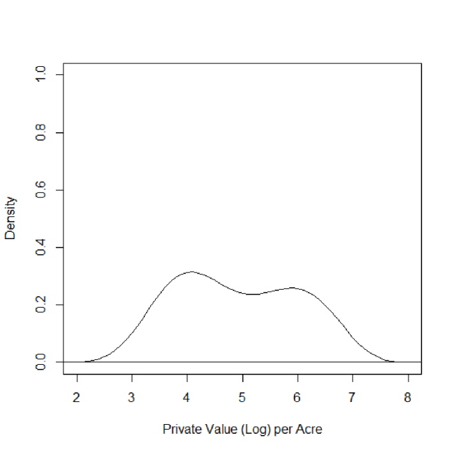
Figure 5. A kernel density estimate of the values $(Y^{(1)},Y^{(2)})$ in the logarithm of US dollars per acre.

References

- Ackerberg et al. (2006) Ackerberg, D.A., Caves, K., and Frazer, G. (2006). Structural identification of production functions. Unpublished manuscript.
- Adusumilli et al. (2016) Adusumilli, K., Otsu, T., and Whang Y.-J. (2016). Inference on distribution functions under measurement error. Unpublished manuscript.
- Armstrong and Kolesár (2017) Armstrong, T. and Kolsár, M. (2017). A simple adjustment for bandwidth snooping. Rev. Econom. Stud., forthcoming.
- Babii (2016) Babii, A. (2016). Honest confidence sets in nonparametric IV regression and other ill-posed models. arXiv:1611.03015.
- Bickel and Rosenblatt (1973) Bickel, P. and Rosenblatt, M. (1973). On some global measures of the deviations of density function estimates. Ann. Statist. 1 1071-1095. Correction (1975) 3 1370.
- Bissantz et al. (2007) Bissantz, N., Dümbgen, L., Holzmann, H., and Munk, A. (2007). Non-parametric confidence bands in deconvolution density estimation. J. R. Stat. Soc. Ser. B. Stat. Methodol. 69 483-506.
- Bissantz and Holzmann (2008) Bissantz, N. and Holzmann, H. (2008). Statistical inference for inverse problems. Inverse Problems 24:034009.
- Bohnomme and Robin (2010) Bohnomme, S. and Robin, J.-M. (2010). Generalized nonparametric deconvolution with an application to earnings dynamics. Rev. Econom. Stud. 77 491-533.
- Bonhomme and Sauder (2011) Bonhomme, S. and Sauder, U. (2011). Recovering distributions in difference-in-differences models: a comparison of selective and comprehensive schooling. Rev. Econ. Stat. 93 479-494.
- Bourdaud et al. (2006) Bourdaud, G., Lanza de Cristoforis, M., and Sickel, W. (2006). Superposition operators and functions of bounded -variation. Rev. Mat. Iberoamericana 22 455-487.
- Calonico et al. (2017) Calonico, S., Cattaneo, M.D., and Farrell, M.H. (2017). On the effect of bias estimation on coverage accuracy in nonparametric inference. J. Amer. Stat. Assoc., forthcoming.
- Carroll and Hall (1988) Carroll, R.J. and Hall, P. (1988). Optimal rates of convergence for deconvolving a density. J. Amer. Statist. Assoc. 83 1184-1186.
- Carroll et al. (2006) Carroll, R.J., Ruppert, D., Stefanski, L.A., and Crainiceanu, C.M. (2006). Measurement Error in Nonlinear Models: A Modern Perspective (2nd Edition). Chapman & Hall/CRC.
- Chen and Christensen (2015) Chen, X. and Christensen, T. (2015). Optimal sup-norm rates, adaptivity and inference in nonparametric instrumental variables estimation. arXiv:1508.03365.
- Chen et al. (2011) Chen X, Hong, H, and Nekipelov, D. (2011). Nonlinear models of measurement errors. J. Econ. Lit. 49 901-937.
- Chernozhukov et al. (2014a) Chernozhukov, V., Chetverikov, D., and Kato, K. (2014a). Gaussian approximation of suprema of empirical processes. Ann. Statist. 42 1564-1597.
- Chernozhukov et al. (2014b) Chernozhukov, V., Chetverikov, D., and Kato, K. (2014b). Anti-concentration and honest, adaptive confidence bands. Ann. Statist. 42 1787-1818.
- Chernozhukov et al. (2015) Chernozhukov, V., Chetverikov, D., and Kato, K. (2015). Comparison and anti-concentration bounds for maxima of Gaussian random vectors. Probab. Theory Related Fields 162 47-70.
- Chernozhukov et al. (2016) Chernozhukov, V., Chetverikov, D., and Kato, K. (2016). Empirical and multiplier bootstraps for suprema of empirical processes of increasing complexity, and related Gaussian couplings. Stochastic Process. Appl., to appear. arXiv:1502:00352.
- Claeskens and Van Keilegom (2003) Claeskens, G. and Van Keilegom, I. (2003). Bootstrap confidence bands for regression curves and their derivatives. Ann. Statist. 31 1852-1884.
- Comte and Lacour (2011) Comte, F. and Lacour, C. (2011). Data-driven density estimation in the presence of additive noise with unknown distribution. J. R. Stat. Soc. Ser. B. Stat. Methodol. 73 601-627.
- Dattner et al. (2016) Dattner, I., Reiß, M., and Trabs, M. (2016). Adaptive quantile estimation in deconvolution with unknown error distribution. Bernoulli 22 143–192.
- Delaigle and Gijbels (2004) Delaigle, A. and Gijbels, I. (2004). Practical bandwidth selection in deconvolution kernel density estimation. Comput. Statist. Data Anal. 45 249-267.
- Delaigle and Hall (2016) Delaigle, A. and Hall, P. (2016). Methodology for nonparametric deconvolution when the error distribution is unknown. J. R. Stat. Soc. Ser. B. Stat. Methodol. 78 231-252.
- Delaigle et al. (2015) Delaigle, A., Hall, P., and Jamshidi, F. (2015). Confidence bands in nonparametric errors-in-variables regression. J. R. Stat. Soc. Ser. B. Stat. Methodol. 77 149-169.
- Delaigle et al. (2008) Delaigle, A., Hall, P., and Meister, A. (2008). On deconvolution with repeated measurements. Ann. Statist. 36 665-685.
- Diggle and Hall (1993) Diggle, P.J. and Hall, P. (1993). A Fourier approach to nonparametric deconvolution of a density estimate. J. Roy. Stat. Soc. Ser. B. Stat. Methodol. 55 523-531.
- Dudley (2002) Dudley, R.M. (2002). Real Analysis and Probability. Cambridge University Press.
- Efromovich (1997) Efromovich, S. (1997). Density estimation for the case of supersmooth measurement error. J. Amer. Stat. Assoc. 92 526-535.