Resonances for open quantum maps
and a fractal uncertainty principle

Abstract.

We study eigenvalues of quantum open baker’s maps with trapped sets given by linear arithmetic Cantor sets of dimensions $\delta\in(0,1)$. We show that the size of the spectral gap is strictly greater than the standard bound $\max(0,{1\over 2}-\delta)$ for all values of $\delta$, which is the first result of this kind. The size of the improvement is determined from a fractal uncertainty principle and can be computed for any given Cantor set. We next show a fractal Weyl upper bound for the number of eigenvalues in annuli, with exponent which depends on the inner radius of the annulus.

Open quantum maps are useful models in the study of scattering phenomena and in particular scattering resonances. They quantize canonical relations on compact symplectic manifolds, giving families of operators defined on finite dimensional Hilbert spaces. This makes them attractive models for numerical experimentation. See §1.4 for an overview of some of the previous results in physics and mathematics literature.

The present paper investigates eigenvalues (related to resonances by (1.4) below) for a family of open quantum maps known as quantum open baker’s maps. The corresponding trapped orbits form Cantor sets. The combinatorial and number theoretic properties of these sets make it possible to prove results on spectral gaps (Theorems 1, 2) which lie well beyond what is known for other models. We also obtain a fractal Weyl upper bound (Theorem 3) and provide numerical results (see §6).

The quantum open baker’s maps we study are determined by triples

$$(M,\mathcal{A},\chi),\quad M\in\mathbb{N},\quad\mathcal{A}\subset\{0,\dots,M-1\},\quad\chi\in C_{0}^{\infty}\big{(}(0,1);[0,1]\big{)}.$$ (1.1)

We call $M$ the base, $\mathcal{A}$ the alphabet, and $\chi$ the cutoff function. For each $k\in\mathbb{N}$, the corresponding open quantum baker’s map is the operator on

$$\ell^{2}_{N}=\ell^{2}(\mathbb{Z}_{N}),\quad\mathbb{Z}_{N}=\mathbb{Z}/(N\mathbb{Z}),\quad N:=M^{k}$$

defined as follows (see §2.1 for details):

$$B_{N}=B_{N,\chi}=\mathcal{F}_{N}^{*}\begin{pmatrix}\chi_{N/M}\mathcal{F}_{N/M}\chi_{N/M}&\\ &\ddots&\\ &&\chi_{N/M}\mathcal{F}_{N/M}\chi_{N/M}\end{pmatrix}I_{\mathcal{A},M}$$ (1.2)

where $\mathcal{F}_{N}$ is the unitary Fourier transform, $\chi_{N/M}$ is the multiplication operator on $\ell^{2}_{N/M}$ discretizing $\chi$, and $I_{\mathcal{A},M}$ is the diagonal matrix with $\ell$-th diagonal entry equal to 1 if $\lfloor{\ell\over N/M}\rfloor\in\mathcal{A}$ and 0 otherwise. A basic example is $M=3$, $\mathcal{A}=\{0,2\}$, giving

$$N=3^{k},\quad B_{N}=\mathcal{F}_{N}^{*}\begin{pmatrix}\chi_{N/3}\mathcal{F}_{N/3}\chi_{N/3}&0&0\\ 0&0&0\\ 0&0&\chi_{N/3}\mathcal{F}_{N/3}\chi_{N/3}\end{pmatrix}.$$

The operator $B_{N}$ is the discrete analog of a Fourier integral operator corresponding to the classical open baker’s map, which is the following symplectic relation on the torus $\mathbb{T}^{2}_{x,\xi}$ (see §2.1 and Figure 1)

$$\begin{gathered}\varkappa_{M,\mathcal{A}}:(y,\eta)\mapsto(x,\xi)=\Big{(}My-a,{\eta+a\over M}\Big{)},\\ (y,\eta)\in\Big{(}{a\over M},{a+1\over M}\Big{)}\times(0,1),\quad a\in\mathcal{A}.\end{gathered}$$ (1.3)

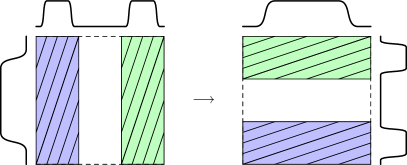
Figure 1. The classical open baker’s map $\varkappa_{M,\mathcal{A}}$ for $M=3,\mathcal{A}=\{0,2\}$, picturing the cutoffs forming the symbol of the Fourier integral operator.

The symbol of the Fourier integral operator has the form $\chi(x)\chi(\eta)$ and cuts off from the boundaries of the rectangles where the transformation $\varkappa_{M,\mathcal{A}}$ is defined. Without the cutoff $\chi$, the operator $B_{N}$ would have additional singularities which would change the spectrum – see §1.3 below.

The linearization of $\varkappa_{M,\mathcal{A}}$ has eigenvalues $M,1/M$. The operator $B_{N}$ is then a toy model for the time $t=\log M$ propagator of a quantum system which has classical expansion rate $1$ (such as a convex co-compact hyperbolic surface, see for instance [DyZa]), at frequencies $\sim N$. In particular, if $\omega$, $\operatorname{Im}\omega\leq 0$, is a scattering resonance for the quantum system, then the corresponding eigenvalue of $B_{N}$ is

$$\lambda=e^{-it\omega}=M^{-i\omega},\quad|\lambda|=M^{\operatorname{Im}\omega}\leq 1.$$ (1.4)

This formula provides an analogy between gap/counting results for scattering resonances and those for eigenvalues of open quantum maps.

We assume that $1<|\mathcal{A}|<M$ and define the parameter

$$\delta:={\log|\mathcal{A}|\over\log M}\in(0,1)$$ (1.5)

which is the dimension of the corresponding Cantor set – see (1.9), (1.16) below. We remark that the topological pressure of the time $t=\log M$ suspension of the map $\varkappa_{M,\mathcal{A}}$ on the trapped set (2.33) is given by [Non, §8.2.2]

$$P(s)=\delta-s,\quad s\in\mathbb{R}.$$ (1.6)

Here we choose time $\log M$ suspension so that it has expansion rate 1, see the discussion preceding (1.4).

1.1. Spectral gaps

The matrix $B_{N}$ has norm bounded by 1, therefore its spectrum $\operatorname{Sp}(B_{N})$ is contained in the unit disk. Our first result shows in particular that the spectral radius of $B_{N}$ is less than 1, uniformly as $N\to\infty$:

Theorem 1 (Improved spectral gap).

There exists

$$\beta=\beta(M,\mathcal{A})>\max\Big{(}0,{1\over 2}-\delta\Big{)}$$ (1.7)

such that

$$\limsup_{N\to\infty}\max\{|\lambda|\colon\lambda\in\operatorname{Sp}(B_{N})\}\ \leq\ M^{-\beta}.$$ (1.8)

The size of the gap (1.7) improves over both the trivial bound and the pressure bound $-P({1\over 2})={1\over 2}-\delta$ (see [Non, §8]) for the entire range $\delta\in(0,1)$. See §1.4 below for an overview of previously known spectral gap results. We also provide a polynomial resolvent bound for $|\lambda|>M^{-\beta}$, see Proposition 4.2.

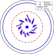
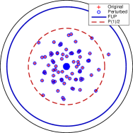
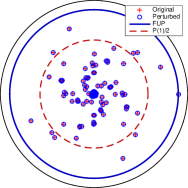
$\mathcal{A}=\{1,2,3\}$ $\mathcal{A}=\{2,3,4\}$ $\mathcal{A}=\{3,4,5\}$

Figure 2. The spectrum of $B_{N}$ for $M=9$, $k=4$, and three different alphabets with $\delta=1/2$. The spectral radius bound (1.8) (labeled ‘FUP’) is close to being sharp for $\mathcal{A}=\{3,4,5\}$ but not for the other two alphabets. We use a small random perturbation to test the stability of the numerics. See §6 for the notation used in the eigenvalue plots.

The constant in (1.7) can be computed as follows. Define the $k$-th order Cantor set

$$\mathcal{C}_{k}=\mathcal{C}_{k}(M,\mathcal{A})=\Big{\{}\sum_{j=0}^{k-1}a_{j}M^{j}\,\Big{|}\,a_{0},\dots,a_{k-1}\in\mathcal{A}\Big{\}}\subset\mathbb{Z}_{N}.$$ (1.9)

Denoting by $\operatorname{1\hskip-2.75ptl}_{\mathcal{C}_{k}}$ the multiplication operator by the indicator function of $\mathcal{C}_{k}$, define

$$r_{k}=\|\operatorname{1\hskip-2.75ptl}_{\mathcal{C}_{k}}\mathcal{F}_{N}\operatorname{1\hskip-2.75ptl}_{\mathcal{C}_{k}}\|_{\ell^{2}_{N}\to\ell^{2}_{N}}.$$ (1.10)

Then Theorem 1 is a corollary of the more precise

Theorem 2.

There exists a limit, called the fractal uncertainty exponent,

$$\beta=\beta(M,\mathcal{A})=-\lim_{k\to\infty}{\log r_{k}\over k\log M}>\max\Big{(}0,{1\over 2}-\delta\Big{)}$$ (1.11)

and (1.8) holds for this choice of $\beta$.

The definition (1.11) implies the following bound, which we call fractal uncertainty principle since it says that no function can be supported on $\mathcal{C}_{k}$ in both position and frequency:

$$\|\operatorname{1\hskip-2.75ptl}_{\mathcal{C}_{k}}\mathcal{F}_{N}\operatorname{1\hskip-2.75ptl}_{\mathcal{C}_{k}}\|_{\ell^{2}_{N}\to\ell^{2}_{N}}\leq C_{\varepsilon}N^{-\beta+\varepsilon}\quad\text{for all }\varepsilon>0.$$ (1.12)

The fractal uncertainty principle implies a bound on the spectral radius of $B_{N}$ by the following argument which previously appeared in the setting of hyperbolic manifolds in [DyZa]: an eigenfunction with eigenvalue $\lambda$, $|\lambda|\geq M^{-\beta+\varepsilon}$, would give a counterexample to (1.12) since (a) it is essentially supported near $\mathcal{C}_{k}$ in frequency and (b) its mass when restricted to near $\mathcal{C}_{k}$ in position has a lower bound. We present the proof in §2; due to the explicit nature of open quantum maps it is greatly simplified on the technical level compared to [DyZa].

Theorems 1 and 2 only give an upper bound on the spectral radius of $B_{N}$. Lower bounds are difficult to prove mathematically because this would involve showing existence of eigenvalues of nonselfadjoint operators. However, numerical evidence suggests that there are cases for which (1.8) is close to being sharp – see Figures 2, 8, 9, and 10. We also remark that the constant $\beta(M,\mathcal{A})$ does not depend on the cutoff $\chi$. The spectral radius of $B_{N}$ may be much smaller than $\beta(M,\mathcal{A})$ for some choices of $\chi$ (for instance $\chi\equiv 0$) however the size of a spectral gap with polynomial resolvent bound is independent of $\chi$ as long as $\chi=1$ near $\mathcal{C}_{\infty}$, see Theorem 4 below.

It is easy to show (1.12) with $\beta=\max(0,{1\over 2}-\delta)$ using only the size of $\mathcal{C}_{k}$, see (3.6). The proof that (1.12) holds for some $\beta>\max(0,{1\over 2}-\delta)$, presented in §§3.1–3.3, is more complicated and uses the algebraic structure of the Cantor sets $\mathcal{C}_{k}$. In particular it relies on a submultiplicative inequality (3.10), which uses that $N$ is a power of $M$ and does not seem to extend to more general situations. More recent results of Bourgain–Dyatlov [BoDy] and Dyatlov–Jin [DyJi] give a fractal uncertainty principle for the much more general class of Ahlfors–David regular sets. They in particular imply that Theorem 1 holds without the assumption $N=M^{k}$ (though with less information on the size of $\beta$) – see [DyJi, §5].

The value of the exponent $\beta$ in (1.11) varies with the choice of the alphabet, even for fixed $M,\delta$ – see Figure 3. We summarize several quantitative results regarding this dependence, valid for large $M$ and proved in §3:

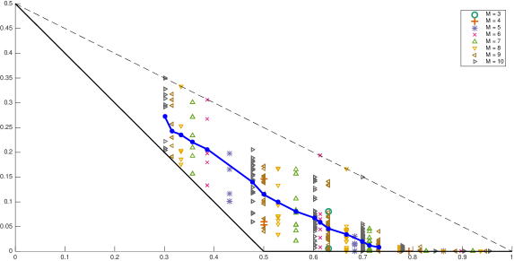
Figure 3. Numerically approximated fractal uncertainty exponents for all possible alphabets with $M\leq 10$. Here the $x$ axis represents $\delta$ and the $y$ axis represents $\beta$. The solid black line is $\beta=\max(0,{1\over 2}-\delta)$ and the dashed line is $\beta={1-\delta\over 2}$. The solid blue line is the average value of $\beta$ over all alphabets with given $M\in[6,10]$ and $\delta\leq 0.75$. See §6 for details.

1. For $\delta\leq{1\over 2}$, the value $\beta-(1/2-\delta)$ is bounded below by a negative power of $M$ – see Corollary 3.5. For $\delta<{1\over 2}$, there exist alphabets for which $\beta-(1/2-\delta)$ is also bounded above by a (different) negative power of $M$ – see Proposition 3.17.

2. For $\delta={1\over 2}+o({1\over\log M})$, $\beta$ is bounded below by ${1\over\mathbf{K}\log M}$ (here $\mathbf{K}$ denotes a global constant) – see Proposition 3.12. In fact, $\beta$ can be estimated in terms of the additive energy of $\mathcal{C}_{k}$. There exist alphabets with $\delta={1\over 2}$ for which $\beta$ is bounded above by $\mathbf{K}\over\log M$ – see Proposition 3.17.

3. For $\delta>{1\over 2}$, $\beta$ is bounded below by

   $$\beta\geq\exp\big{(}-M^{{\delta\over 1-\delta}+o(1)}\big{)},$$

   see Corollary 3.7. We do not prove matching upper bounds but numerical evidence in Table 1 suggests that there exists alphabets with $\beta$ exponentially small in $M$.

4. We always have

   $$\beta\leq{1-\delta\over 2}=-{P(1)\over 2},$$ (1.13)

   corresponding to the classical escape rate (see §1.4 and (3.30)), and for a generic alphabet the inequality in (1.13) is strict – see Proposition 3.16. However, there exist infinitely many pairs $(M,\mathcal{A})$ for which $\beta={1-\delta\over 2}$, see §3.5. Numerical evidence suggests that for these special alphabets the spectrum of $B_{N}$ has a band structure, making it the most feasible case for proving a fractal Weyl asymptotic for the number of eigenvalues – see Conjecture 3.14.

5. Finally, the expected value of $\beta$ for large $M$ and a randomly chosen $\mathcal{A}$ of fixed size appears to be much larger than $\max(0,{1\over 2}-\delta)$, see the solid blue line on Figure 3. A related question of $L^{p}$ Fourier restriction bounds for random sets was investigated by Bourgain [Bou]. Examples of random multiscale Cantor sets satisfying $L^{p}$ restriction bounds and Fourier decay estimates were constructed by Chen–Seeger [ChSe], Shmerkin–Suomala [ShSu], and Łaba–Wang [ŁaWa].

1.2. Weyl bounds

Our next result concerns the counting function

$$\mathcal{N}_{k}(\nu)=\big{|}\operatorname{Sp}(B_{N})\cap\{|\lambda|\geq M^{-\nu}\}\big{|},\quad\nu\geq 0,$$ (1.14)

where eigenvalues of $B_{N}$ are counted with multiplicities. We obtain a Weyl upper bound on $\mathcal{N}_{k}(\nu)$ (see [Non, §6.1]):

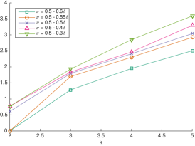
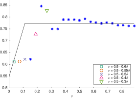
Figure 4. Left: plot of $\log\mathcal{N}_{k}(\nu)/\log M$ for $M=6$, $\mathcal{A}=\{1,2,3,4\}$, as a function of $k=2,\dots,5$ and for various values of $\nu$. We have $\delta=\log 4/\log 6\approx 0.7737$. Right: the slope of best linear approximation to the graph on the left restricted to $k=3,4,5$, as a function of $\nu$, together with the bound $m(\delta,\nu)$ of Theorem 3.

Theorem 3 (Weyl bounds).

For each $\nu>0$ and $\varepsilon>0$, we have as $k\to\infty$

$$\mathcal{N}_{k}(\nu)=\mathcal{O}(N^{m(\delta,\nu)+\varepsilon}),\quad m(\delta,\nu)=\min(2\nu+2\delta-1,\delta).$$ (1.15)

The proof, presented in §4, uses the argument introduced for hyperbolic surfaces in [Dy15b]. Note that $m(\delta,\nu)=\delta$ for $\nu\geq{1-\delta\over 2}$, corresponding to the standard Weyl law (see §1.4). For $\nu\leq{1-\delta\over 2}$, the exponent $m(\delta,\nu)$ interpolates linearly between $m(\delta,{1-\delta\over 2})=\delta$ and $m(\delta,{1\over 2}-\delta)=0$, the latter corresponding to the pressure gap.

While no matching lower bounds on $\mathcal{N}_{k}(\nu)$ are known rigorously, numerical evidence on Figure 4 suggests that $\mathcal{N}_{k}(\nu)\sim N^{\delta}$ for $\nu$ large enough. However, because of the small number of data points available (and the resulting artefacts such as rough behavior of the exponents in the right half of Figure 4) we could not determine how close (1.15) is to the optimal bound.

1.3. Dependence on cutoff

Our final result, proved in §5, concerns the dependence of the spectrum of $B_{N,\chi}$ on the cutoff $\chi$. Let $\mathcal{C}_{\infty}\subset[0,1]$ be the limiting Cantor set:

$$\mathcal{C}_{\infty}=\bigcap_{k}\bigcup_{j\in\mathcal{C}_{k}}\Big{[}{j\over M^{k}},{j+1\over M^{k}}\Big{]}.$$ (1.16)

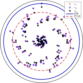
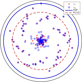
Figure 5. An illustration of Theorem 4, with $M=4$, $\mathcal{A}=\{1,2\}$, $k=6$. We take cutoffs $\chi_{1},\chi_{2},\chi_{3},\chi_{4}$ such that $\chi_{1},\chi_{2},\chi_{3}\in C_{0}^{\infty}((0,1);[0,1])$, $\chi_{1}=\chi_{2}=1$ on $\mathcal{C}_{\infty}$, $\chi_{3}\not\equiv 1$ on $\mathcal{C}_{\infty}$, and $\chi_{4}\equiv 1$. On the left, we see that $\chi_{1}$ and $\chi_{2}$ produce essentially the same eigenvalues, but $\chi_{3}$ does not. On the right, we see that sufficiently small eigenvalues for $\chi_{4}$ are significantly different than those for $\chi_{1}$; this is due to the fact that the Fourier transform of the sharp cutoff $\chi_{4}=\mathbf{1}_{[0,1]}$ is not rapidly decaying.

Theorem 4 (Dependence on cutoff).

Assume that $\chi,\chi^{\prime}\in C_{0}^{\infty}((0,1);[0,1])$ satisfy

$$\chi=\chi^{\prime}\quad\text{in a neighborhood of }\mathcal{C}_{\infty}.$$

Fix $\nu\geq 0$ and assume that $\lambda$ is an eigenvalue of $B_{N,\chi}$ satisfying $|\lambda|\geq M^{-\nu}$. Then there exists an $\mathcal{O}(N^{-\infty})$ quasimode $v$ for $B_{N,\chi^{\prime}}$ at $\lambda$, that is

$$v\in\ell^{2}_{N},\quad\|v\|_{\ell^{2}_{N}}=1,\quad\|(B_{N,\chi^{\prime}}-\lambda)v\|_{\ell^{2}_{N}}=\mathcal{O}(N^{-\infty}),$$

with the constants in $\mathcal{O}(N^{-\infty})$ depending only on $\chi,\chi^{\prime},\nu$.

Theorem 4 does not imply that the spectra of $B_{N,\chi}$ and $B_{N,\chi^{\prime}}$ in annuli are $\mathcal{O}(N^{-\infty})$ close to each other, due to possible pseudospectral effects. However, it shows that for stable features of the spectrum such as eigenvalue free regions with a polynomial resolvent bound, only the values of $\chi$ near $\mathcal{C}_{\infty}$ matter. In particular, if $0,M-1\notin\mathcal{A}$, then one can choose an arbitrary $\chi$ such that $\chi=1$ near $\mathcal{C}_{\infty}$ and see the same stable properties of the spectrum. A numerical illustration of Theorem 4 is shown on Figure 5.

1.4. Related results

We now briefly review some previous results in resonance gaps and counting and explain their relation to the present paper. For more information we refer the reader to Nonnenmacher [Non] for mathematical results in open quantum chaos, to Novaes [Nov] for the physics literature on open quantum maps, and to Zelditch [Ze] for the closely related field of closed quantum chaos.

A popular class of models for open quantum chaos is given by Laplacians (or more general Schrödinger operators) on noncompact Riemannian manifolds whose geodesic flow is hyperbolic on the trapped set. Resonances for these operators appear in long time expansions of solutions to wave equations. Examples include exteriors of several convex obstacles in $\mathbb{R}^{n}$ and convex co-compact hyperbolic quotients. We remark that [NSZ11] reduced the study of resonances for Laplacians to the setting of open quantum maps quantizing a Poincaré map of the geodesic flow.

Essential spectral gaps for Laplacians have been studied by Patterson [Pa], Ikawa [Ik], Gaspard–Rice [GaRi], and Nonnenmacher–Zworski [NoZw09]. These papers establish in various settings a gap of size $\beta=-P(1/2)$, under the pressure condition $P(1/2)<0$. Here $P(s)$ is the topological pressure of the classical flow, see (1.6). The pressure gap was observed in microwave scattering experiments by Barkhofen et al. [BWPSKZ].

Naud [Na05], Stoyanov [St11, St12], and Petkov–Stoyanov [PeSt] showed that in some cases such as hyperbolic quotients, there exists a gap strictly larger than $-P(1/2)$, under the condition $P(1/2)\leq 0$. These works use the method originally developed by Dolgopyat [Do], exploiting in a subtle way the interference between waves living on different trapped trajectories, and the size of the improvement is hard to compute from the arguments. Recently Dyatlov–Zahl [DyZa] have come up with a different interpretation of the improved gap for hyperbolic quotients in terms of fractal uncertainty principle, in particular obtaining for $P(1/2)\approx 0$ a gap whose size depends on the additive energy of the limit set similarly to §3.4. The approach of [DyZa] is used in the present paper as well as in the recent papers [BoDy, DyJi] discussed in §1.1. Improved gaps were also observed numerically for hyperbolic surfaces with $P(1/2)\approx 0$ by Borthwick and Borthwick–Weich [Bor, BoWe].

On the other hand very little is known about spectral gaps for systems with $P(1/2)>0$ and Theorem 1 appears to be the first general result in this case, albeit for a special class of systems. Examples of systems with $P(1/2)>0$ and a spectral gap were previously given in [NoZw07], discussed below, and [DyZa].

Fractal Weyl upper bounds in strips for resonances of Laplacians and Schrödinger operators were first proved in the analytic category by Sjöstrand [Sj] and later in various smooth settings by Guillopé–Lin–Zworski [GLZ], Zworski [Zw99], Sjöstrand–Zworski [SjZw], Nonnenmacher–Sjöstrand–Zworski [NSZ11, NSZ14], and Datchev–Dyatlov [DaDy]. In terms of (1.14) these bounds give $\mathcal{N}_{k}(\nu)=\mathcal{O}(N^{\delta})$, with $\delta$ related to the Minkowski dimension of the trapped set. Compared to these works, our bound (1.15) loses an arbitrarily small power of $N$. The sharpness of the exponent $\delta$ has been investigated experimentally by Potzuweit et al. [PWBKSZ] and numerically by Lu–Sridhar–Zworski [LSZ], Borthwick [Bor], Borthwick–Weich [BoWe], and Borthwick–Dyatlov–Weich [Dy15b, Appendix].

Concentration of resonances near the decay rate $P(1)/2$ has been observed numerically in [LSZ] and experimentally in [BWPSKZ, PWBKSZ]. Jakobson–Naud [JaNa] conjectured that for hyperbolic surfaces, there is a gap of any size less than $P(1)/2$. While the numerical investigations of [Bor, BoWe, Dy15b] do not seem to support this conjecture for general systems, in §3.5 we provide examples of systems which do satisfy the conjecture. Naud [Na14] showed an improved Weyl bound $\mathcal{N}_{k}(\nu)=\mathcal{O}(N^{m(\nu)})$ for hyperbolic surfaces, for some $m(\nu)<\delta$ when $\nu<P(1)/2$, and Dyatlov [Dy15b] proved the bound (1.15) for hyperbolic quotients.

Quantum baker’s maps have attracted a lot of attention in physics and mathematics literature. Their study was initiated in the closed setting $\mathcal{A}=\{0,\dots,M-1\}$ by Balázs–Voros [BaVo], Saraceno [Sa], and Saraceno–Voros [SaVo]; see the introduction to [DNW] for an overview of more recent results. In the open setting, Keating et al. [KNPS] observed numerically concentration of eigenfunctions in position and momentum consistent with Proposition 2.5. This concentration was proved for the Walsh quantization by Keating et al. [KNNS]; see also the work of Nonnenmacher–Rubin [NoRu] on semiclassical defect measures. Novaes et al. [NPWCK] and Carlo–Benito–Borondo [CBB] introduced an approximation for eigenfunctions using short periodic orbits. Experimental realizations for open baker’s maps have been proposed by Brun–Schack [BrSc] and Hannay–Keating–Ozorio de Almeida [HKO]. Recently ideas in open quantum chaos have been applied to analysis of computer networks, see Ermann–Frahm–Shepelyansky [EFS].

The closest to the present paper is the work of Nonnenmacher–Zworski [NoZw05, NoZw07] who studied open quantum baker’s maps, in particular the Walsh quantization for the cases $M=3,4$, $\mathcal{A}=\{0,2\}$, $\chi\equiv 1$ in the notation of our paper (as well as obtaining numerical results for other maps and quantizations). The Walsh quantization is obtained by replacing $\mathcal{F}_{N},\mathcal{F}_{N/M}$ in (1.2) by the Walsh Fourier transform, which is the Fourier transform on the group $(\mathbb{Z}_{M})^{k}$. Eigenvalues of Walsh quantizations are computed explicitly in [NoZw07, §5], which proves fractal Weyl law and shows concentration of resonances around decay rate $P(1)/2$. Moreover [NoZw07] shows that there is a spectral gap for $M=3,\mathcal{A}=\{0,2\}$ but not for $M=4,\mathcal{A}=\{0,2\}$. The latter does not contradict Theorem 1 because a different quantization is used, and Cantor sets do not always satisfy the uncertainty principle under the Walsh Fourier transform.

2. Open quantum maps

In this section, we study the open quantum map $B_{N}$. The main result is Proposition 2.6, giving a bound on the spectral radius of $B_{N}$ in terms of the fractal uncertainty principle exponent $\beta$ defined in (1.11).

2.1. Definition and basic properties

For $N\in\mathbb{N}$, consider the abelian group

$$\mathbb{Z}_{N}=\mathbb{Z}/N\mathbb{Z}\simeq\{0,\dots,N-1\}$$

and the space $\ell^{2}_{N}$ of functions $u:\mathbb{Z}_{N}\to\mathbb{C}$ with the Hilbert norm

$$\|u\|_{\ell^{2}_{N}}^{2}=\sum_{j=0}^{N-1}|u(j)|^{2}.$$

Define the unitary Fourier transform

$$\mathcal{F}_{N}:\ell^{2}_{N}\to\ell^{2}_{N},\quad\mathcal{F}_{N}u(j)={1\over\sqrt{N}}\sum_{\ell=0}^{N-1}\exp\Big{(}-{2\pi ij\ell\over N}\Big{)}u(\ell).$$

For a cutoff function $\chi\in C_{0}^{\infty}((0,1);[0,1])$, define its discretization $\chi_{N}\in\ell^{2}_{N}$ by

$$\chi_{N}(j)=\chi\Big{(}{j\over N}\Big{)},\quad j\in\{0,\dots,N-1\}.$$ (2.1)

We also denote by $\chi_{N}$ the corresponding multiplication operator on $\ell^{2}_{N}$.

Fix $(M,\mathcal{A},\chi)$ as in (1.1) and take $k\in\mathbb{N}$; put $N:=M^{k}$. Then the open quantum map $B_{N}:\ell^{2}_{N}\to\ell^{2}_{N}$ defined in (1.2) can be written as follows: if $\Pi_{a}:\ell^{2}_{N}\to\ell^{2}_{N/M}$, $a\in\{0,\dots,M-1\}$, is the projection map defined by

$$\Pi_{a}u(j)=u\Big{(}j+a{N\over M}\Big{)},\quad u\in\ell^{2}_{N},\quad j\in\Big{\{}0,\dots,{N\over M}-1\Big{\}},$$ (2.2)

then

$$B_{N}=\sum_{a\in\mathcal{A}}B_{N}^{a},\quad B_{N}^{a}:=\mathcal{F}_{N}^{*}\Pi_{a}^{*}\,\chi_{N/M}\,\mathcal{F}_{N/M}\,\chi_{N/M}\,\Pi_{a}.$$

We compute for each $u\in\ell^{2}_{N}$, $j\in\{0,\dots,N-1\}$, and $a\in\mathcal{A}$,

$$B_{N}^{a}u(j)={\sqrt{M}\over N}\sum_{m,\ell=0}^{{N\over M}-1}e^{2\pi i\left({(j-M\ell)m\over N}+{ja\over M}\right)}\chi\Big{(}{mM\over N}\Big{)}\chi\Big{(}{\ell M\over N}\Big{)}u\Big{(}\ell+a{N\over M}\Big{)}.$$ (2.3)

The continuous analogue of the transformation $B_{N}$ is obtained as follows: put

$$x:={j\over N},\quad y:={\ell\over N}+{a\over M},\quad\theta:={m\over N},\quad h:={1\over 2\pi N}$$

and replace the sums over $\ell,m$ by integrals over $y,\theta$ with the corresponding Jacobian factors. Then the analogue of (2.3) is given by the operator $\mathcal{U}^{a}_{h}$ on $L^{2}(\mathbb{R})$ defined as follows:

$$\mathcal{U}^{a}_{h}v(x)={\sqrt{M}\over 2\pi h}\int_{\mathbb{R}^{2}}e^{{i\over h}\left((x+a-My)\theta+xa/M\right)}\chi(M\theta)\chi(My-a)u(y)\,dyd\theta.$$ (2.4)

The sum

$$\mathcal{U}_{h}:=\sum_{a\in\mathcal{A}}\mathcal{U}^{a}_{h}$$ (2.5)

is a semiclassical Fourier integral operator (see for instance [Dy15a, §3.2]) associated to the canonical relation $\varkappa_{M,\mathcal{A}}$ defined in (1.3), with principal symbol equal to $\chi(x)\chi(\eta)$ with appropriate normalization. Because of the analogy with the continuous case, we may think of $B_{N}$ as a discrete Fourier integral operator quantizing the relation $\varkappa_{M,\mathcal{A}}$. A rigorous justification of this analogy can be found in the papers of Degli Esposti–Nonnenmacher–Winn [DNW] and Nonnenmacher–Zworski [NoZw07], with heuristic arguments appearing in Balázs–Voros [BaVo] and Saraceno–Voros [SaVo].

We next consider the distance function on $[0,1]$ with $0$ and $1$ identified with each other: for $x,y\in[0,1]$,

$$d(x,y)=\min_{k=-1,0,1}|x-y-k|=\min\{|x-y|,1-|x-y|\}.$$

In particular, $d(x,0)=\min\{x,1-x\}$ is the usual distance from $x$ to the closest integer. For $x\in[0,1]$ and $V,W\subset[0,1]$, we put

$$d(x,V):=\inf_{y\in V}d(x,y),\quad d(V,W):=\inf_{y\in V,\,z\in W}d(y,z).$$ (2.6)

We define the expanding map

$$\begin{gathered}\Phi=\Phi_{M,\mathcal{A}}:\bigsqcup_{a\in\mathcal{A}}\left(\frac{a}{M},\frac{a+1}{M}\right)\to(0,1);\\ \Phi(x)=Mx-a,\quad x\in\left(\frac{a}{M},\frac{a+1}{M}\right).\end{gathered}$$ (2.7)

In other words, $\Phi_{M,\mathcal{A}}$ is the action of the relation $\varkappa_{M,\mathcal{A}}$ on the space variable $x$. We establish the following fact regarding the interaction between the map $\Phi$ and the distance function $d$:

Lemma 2.1.

Assume that $x\in[0,1]$ and $y$ is in the domain of $\Phi$. Then

$$\min\big{\{}d(\Phi(y),0),\,M\cdot d(y,\Phi^{-1}(x))\big{\}}\leq d(x,\Phi(y)).$$ (2.8)

Proof.

We have the following equivalent expression for $d(x,y)$:

$$d(x,y)=\min\{|x-y|,d(x,0)+d(y,0)\}.$$

Therefore

$$d(x,\Phi(y))=\min\big{\{}|x-\Phi(y)|,d(x,0)+d(\Phi(y),0)\big{\}}.$$

Let $\tilde{x}$ be the unique element in $\Phi^{-1}(x)$ that is in the same interval $({a\over M},{a+1\over M})$ as $y$. Then

$$|x-\Phi(y)|=M|\tilde{x}-y|\geq Md(y,\Phi^{-1}(x)),$$

finishing the proof. ∎

We also use the following result on rapid decay for oscillating sums, which is the discrete analog of rapid decay of Fourier series of smooth functions:

Lemma 2.2 (Method of nonstationary phase).

Assume that $a\in\mathbb{Z}_{N}$ and

$$d\Big{(}{a\over N},0\Big{)}\geq cN^{-\rho}\quad\text{for some constants }c>0,\ \rho\in[0,1).$$ (2.9)

Then for all $\chi\in C_{0}^{\infty}((0,1))$, we have

$$\sum_{m=0}^{N-1}\exp\Big{(}{2\pi iam\over N}\Big{)}\chi\Big{(}{m\over N}\Big{)}=\mathcal{O}(N^{-\infty})$$ (2.10)

where the constants in $\mathcal{O}(N^{-\infty})$ only depend on $c$, $\rho$, and $\chi$.

Proof.

Applying the Poisson summation formula to the function $e^{2\pi iax/N}\chi(x/N)$, we write the left-hand side of (2.10) as

$$N\sum_{\ell\in\mathbb{Z}}\hat{\chi}(N\ell-a)$$

where $\hat{\chi}$ is the Fourier transform of $\chi$:

$$\hat{\chi}(\xi)=\int_{\mathbb{R}}\exp(-2\pi ix\xi)\chi(x)\,dx.$$

Since $\hat{\chi}$ is rapidly decreasing, (2.10) follows; here we use (2.9) to handle the cases $\ell=0,1$. ∎

2.2. Propagation of singularities

Following (2.1), for each $\varphi:[0,1]\to\mathbb{R}$, we define

$$\varphi_{N}\in\ell^{2}_{N},\quad\varphi_{N}(j)=\varphi\Big{(}{j\over N}\Big{)}.$$

The function $\varphi_{N}$ defines a multiplication operator on $\ell^{2}_{N}$, still denoted $\varphi_{N}$. We also use the corresponding Fourier multplier

$$\varphi_{N}^{\mathcal{F}}=\mathcal{F}_{N}^{*}\varphi_{N}\mathcal{F}_{N}.$$

The following theorems are analogues of propagation of semiclassical singularities (that is, regions where $\varphi_{N}$ is not $\mathcal{O}(N^{-\infty})$) in position and frequency space under quantum evolution. A stronger statement (not needed here) is Egorov’s theorem, which describes symbols of propagated quantum observables. In the context of quantum baker’s maps it was proved in [DNW, Theorems 12,13] and [NoZw07, Proposition 4.15].

We start with the case when we apply the open quantum map only once. We use the map $\Phi$ defined in (2.7) and the cutoff function $\chi$ which is part of (1.1). Note that due to the simple nature of the map $B_{N}$ we do not need to impose any smoothness assumptions on the classical observables $\varphi,\psi$ below.

Proposition 2.3 (Propagation of singularities).

Assume that $\varphi,\psi:[0,1]\to[0,1]$ and for some $c>0$ and $0\leq\rho<1$,

$$d\big{(}\Phi(\operatorname{supp}\psi\cap\Phi^{-1}(\operatorname{supp}\chi)),\operatorname{supp}\varphi)\geq cN^{-\rho}.$$ (2.11)

Then

$$\|\varphi_{N}B_{N}\psi_{N}\|_{\ell^{2}_{N}\to\ell^{2}_{N}} =\mathcal{O}(N^{-\infty}),$$ (2.12)

$$\|\psi_{N}^{\mathcal{F}}B_{N}\varphi_{N}^{\mathcal{F}}\|_{\ell^{2}_{N}\to\ell^{2}_{N}} =\mathcal{O}(N^{-\infty}),$$ (2.13)

where the constants in $\mathcal{O}(N^{-\infty})$ depend only on $c,\rho,\chi$. In particular, (2.12) and (2.13) hold when

$$d\big{(}\operatorname{supp}\psi,\Phi^{-1}(\operatorname{supp}\varphi)\big{)}\geq cN^{-\rho}.$$ (2.14)

Remark. The continuous analog of the operator $\varphi_{N}$ is the multiplication operator $\varphi(y)$, and the continuous analog of $\varphi_{N}^{\mathcal{F}}$ is the Fourier multiplier $\varphi({h\over i}\partial_{y})$. Both of these are semiclassical pseudodifferential operators (see for instance [Zw12, §4.1]), with symbols given by $\tilde{\varphi}(y,\eta)=\varphi(y)$ and $\tilde{\varphi}^{\mathcal{F}}(y,\eta)=\varphi(\eta)$. The condition (2.11) is equivalent to each of the following conditions featuring the relation $\varkappa=\varkappa_{M,\mathcal{A}}$ defined in (1.3) and the symbol $\widetilde{\chi}(y,\eta)=\chi(\Phi(y))\chi(\eta)$:

$$d\big{(}\varkappa(\operatorname{supp}\tilde{\psi}\cap\operatorname{supp}\widetilde{\chi}),\operatorname{supp}\tilde{\varphi}\big{)} \geq cN^{-\rho},$$ (2.15)

$$d\big{(}\varkappa^{-1}(\operatorname{supp}\tilde{\psi}^{\mathcal{F}}\cap\varkappa(\operatorname{supp}\widetilde{\chi})),\operatorname{supp}\tilde{\varphi}^{\mathcal{F}}) \geq cN^{-\rho}.$$ (2.16)

The continuous analogues of (2.12), (2.13) are expressed via the operator from (2.5):

$$\varphi\,\mathcal{U}_{h}\psi,\ \psi\Big{(}{h\over i}\partial_{y}\Big{)}\mathcal{U}_{h}\,\varphi\Big{(}{h\over i}\partial_{y}\Big{)}=\mathcal{O}(h^{\infty})_{L^{2}(\mathbb{R})\to L^{2}(\mathbb{R})}$$

In the case when $\varphi,\psi$ are smooth and $h$-independent and $\rho=0$, the latter two statements follow from (2.15), (2.16), and the wavefront set statement (see for instance [Dy15a, §3.2])

$$\operatorname{WF}_{h}(\mathcal{U}_{h})\subset\{(x,\xi;y,\eta)\mid(x,\xi)=\varkappa(y,\eta),\quad(y,\eta)\in\operatorname{supp}\widetilde{\chi}\}.$$

Proof of Proposition 2.3.

By (2.3), we have for all $u\in\ell^{2}_{N}$, $j\in\{0,\dots,N-1\}$,

$$\varphi_{N}B_{N}\psi_{N}u(j) =\sum_{a\in\mathcal{A}}\sum_{\ell=0}^{{N/M}-1}A^{a}_{j\ell}\,u\Big{(}\ell+a{N\over M}\Big{)},$$

$$A^{a}_{j\ell} ={\sqrt{M}\over N}\varphi\Big{(}{j\over N}\Big{)}\exp\Big{(}{2\pi iaj\over M}\Big{)}\chi\Big{(}{\ell M\over N}\Big{)}\psi\Big{(}{\ell\over N}+{a\over M}\Big{)}\widetilde{A}_{j\ell},$$

$$\widetilde{A}_{j\ell} =\sum_{m=0}^{N/M-1}\exp\Big{(}{2\pi im(j-\ell M)\over N}\Big{)}\chi\Big{(}{mM\over N}\Big{)}.$$

We write

$$\widetilde{A}_{j\ell}=\sum_{m=0}^{N-1}\exp\Big{(}{2\pi ibm\over N}\Big{)}\chi_{1}\Big{(}{m\over N}\Big{)},\quad b:=j-\ell M,\quad\chi_{1}(x)=\chi(Mx).$$

We have $A^{a}_{j\ell}=0$ unless

$${j\over N}\in\operatorname{supp}\varphi,\quad{\ell\over N}+{a\over M}\in\operatorname{supp}\psi,\quad{\ell M\over N}=\Phi\Big{(}{\ell\over N}+{a\over M}\Big{)}\in\operatorname{supp}\chi.$$ (2.17)

By (2.11), we see that (2.17) implies

$$d\Big{(}{b\over N},0\Big{)}=d\Big{(}{j\over N},{\ell M\over N}\Big{)}\geq cN^{-\rho}.$$

Applying Lemma 2.2, we see that

$$\max_{a,j,\ell}|A^{a}_{j\ell}|=\mathcal{O}(N^{-\infty})$$

and (2.12) follows.

To show (2.13), we notice that $\mathcal{F}_{N}^{*}=\overline{\mathcal{F}_{N}}$ and thus

$$\psi_{N}^{\mathcal{F}}B_{N}\varphi_{N}^{\mathcal{F}}=\mathcal{F}_{N}^{\ast}(\overline{\varphi_{N}B_{N}\psi_{N}})^{*}\mathcal{F}_{N}$$

where for any operator $A:\ell^{2}_{N}\to\ell^{2}_{N}$ its complex conjugate $\overline{A}:\ell^{2}_{N}\to\ell^{2}_{N}$ is defined by $\overline{A}\,\bar{u}=\overline{Au}$, $u\in\ell^{2}_{N}$. Since both $\mathcal{F}_{N}$ and $\mathcal{F}_{N}^{\ast}$ are unitary, (2.13) follows from (2.12) and the facts that both operations of the complex conjugate and the adjoint preserve the operator norm.

Finally, we show that (2.14) implies (2.11) with a different $c$. Indeed, assume (2.14) holds. Then for any $x\in\operatorname{supp}\varphi$ and $y\in\operatorname{supp}\psi\cap\Phi^{-1}(\operatorname{supp}\chi)$, by (2.8), we see that

$$d(x,\Phi(y)) \geq\min\{d(\Phi(y),0),M\cdot d(y,\Phi^{-1}(x))\}$$

$$\geq\min\{d(\operatorname{supp}\chi,0),cMN^{-\rho}\}\geq c^{\prime}N^{-\rho}$$

which finishes the proof. ∎

Now we turn to the case when we iterate the open quantum map up to (almost) twice the Ehrenfest time $k$.

Proposition 2.4 (Propagation of singularities for long times).

Assume that $\varphi,\psi:[0,1]\to[0,1]$ and for some $c>0$, $0\leq\rho<1$, and an integer $\tilde{k}\in[1,k]$,

$$d\big{(}\operatorname{supp}\psi,\Phi^{-\tilde{k}}(\operatorname{supp}\varphi)\big{)}\geq cN^{-\rho}.$$ (2.18)

Then

$$\|\varphi_{N}(B_{N})^{\tilde{k}}\psi_{N}\|_{\ell^{2}_{N}\to\ell^{2}_{N}} =\mathcal{O}(N^{-\infty}),$$ (2.19)

$$\|\psi_{N}^{\mathcal{F}}(B_{N})^{\tilde{k}}\varphi_{N}^{\mathcal{F}}\|_{\ell^{2}_{N}\to\ell^{2}_{N}} =\mathcal{O}(N^{-\infty}),$$ (2.20)

where the constants in $\mathcal{O}(N^{-\infty})$ depend only on $c,\rho,\chi$.

Proof.

It suffices to construct a sequence of functions (see Figure 6)

$$\varphi^{(j)}:[0,1]\to[0,1],\quad\psi^{(j)}:=1-\varphi^{(j)},\quad j=0,\dots,\tilde{k},$$

such that for some $c^{\prime}>0$ depending only on $c,\chi$,

$$\psi^{(0)}\varphi=0,$$ (2.21)

$$\psi^{(\tilde{k})}\psi=\psi,$$ (2.22)

$$d\big{(}\Phi(\operatorname{supp}\psi^{(j+1)}\cap\Phi^{-1}(\operatorname{supp}\chi)),\operatorname{supp}\varphi^{(j)}\big{)}\geq c^{\prime}N^{-\rho},\quad j=0,\dots,\tilde{k}-1.$$ (2.23)

Indeed, inserting $\operatorname{1\hskip-2.75ptl}=\varphi^{(j)}_{N}+\psi^{(j)}_{N}$ after the $j$-th factor $B_{N}$ and using (2.21), (2.22), we write

$$\begin{gathered}\varphi_{N}(B_{N})^{\tilde{k}}\psi_{N}=\sum_{j=0}^{\tilde{k}-1}A^{\prime}_{j}\big{(}\varphi^{(j)}_{N}B_{N}\psi^{(j+1)}_{N}\big{)}A^{\prime\prime}_{j},\\ A^{\prime}_{j}=\varphi_{N}(B_{N})^{j},\quad A^{\prime\prime}_{j}=(B_{N}\psi_{N}^{(j+2)})\cdots(B_{N}\psi_{N}^{(\tilde{k})})\psi_{N}.\end{gathered}$$

Clearly,

$$\|A^{\prime}_{j}\|_{\ell^{2}_{N}\to\ell^{2}_{N}},\|A^{\prime\prime}_{j}\|_{\ell^{2}_{N}\to\ell^{2}_{N}}\leq 1.$$

Applying (2.12) and using (2.23), we get

$$\|\varphi^{(j)}_{N}B_{N}\psi^{(j+1)}_{N}\|_{\ell^{2}_{N}\to\ell^{2}_{N}}=\mathcal{O}(N^{-\infty}).$$

This concludes the proof of (2.19) as $\tilde{k}\leq k=O(\log N)$. The other estimate (2.20) follows from (2.13) by the same argument.

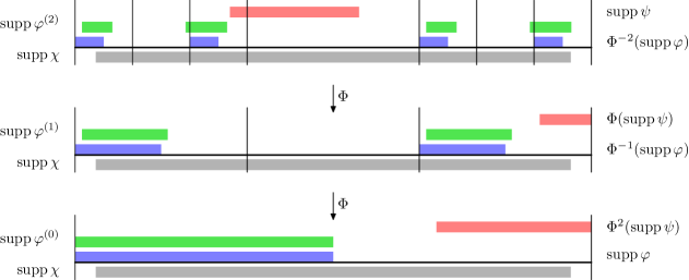
Figure 6. An illustration of the proof of Proposition 2.4 for $M=3$, $\mathcal{A}=\{0,2\}$, $\tilde{k}=2$. Note that $d(\Phi^{2}(\operatorname{supp}\psi),\operatorname{supp}\varphi)=0$, explaining why we need to use the cutoff function $\chi$ in (2.23).

We now construct the functions $\varphi^{(j)}$. Fix $c^{\prime}>0$ depending only on $c,\chi$, to be chosen in (2.26), (2.27) below. Define

$$\varphi^{(0)}(x)=\begin{cases}1,&x\in\operatorname{supp}\varphi,\\ 0,&\text{otherwise}.\end{cases}$$

Note that (2.21) holds. We next define inductively for $j=1,\dots,\tilde{k}$,

$$\varphi^{(j)}(x)=\begin{cases}1,&x\in\Phi^{-1}(\operatorname{supp}\chi)\quad\text{and}\quad d(\Phi(x),\operatorname{supp}\varphi^{(j-1)})\leq c^{\prime}N^{-\rho},\\ 0,&\text{otherwise}.\end{cases}$$

Then (2.23) holds, so it remains to prove (2.22). The latter follows from the fact that

$$\operatorname{supp}\varphi^{(\tilde{k})}\cap\operatorname{supp}\psi=\emptyset.$$ (2.24)

To show (2.24), we note that any point in $\operatorname{supp}\varphi^{(\tilde{k})}$ is equal to $x_{\tilde{k}}$ for some sequence of points $x_{0},\dots,x_{\tilde{k}}\in[0,1]$ such that

$$x_{0}\in\operatorname{supp}\varphi;\quad x_{j}\in\Phi^{-1}(\operatorname{supp}\chi),\quad d(\Phi(x_{j}),x_{j-1})\leq c^{\prime}N^{-\rho},\quad j=1,\dots,\tilde{k}.$$

By (2.18) it then suffices to prove that

$$d(x_{\tilde{k}},\Phi^{-\tilde{k}}(x_{0}))<cN^{-\rho}.$$ (2.25)

We have for each $j=1,\dots,\tilde{k}$,

$$\min\big{\{}d(\operatorname{supp}\chi,0),M\cdot d(x_{j},\Phi^{-j}(x_{0}))\big{\}} \leq\min\big{\{}d(\Phi(x_{j}),0),M\cdot d(x_{j},\Phi^{-j}(x_{0}))\big{\}}$$

$$\leq d(\Phi(x_{j}),\Phi^{-(j-1)}(x_{0}))$$

$$\leq d(x_{j-1},\Phi^{-(j-1)}(x_{0}))+c^{\prime}N^{-\rho}$$

where on the second line we use (2.8). By induction on $j$, we see that if $c^{\prime}$ is small enough so that

$${c^{\prime}M\over M-1}\leq d(\operatorname{supp}\chi,0)$$ (2.26)

then for all $j=0,\dots,\tilde{k}$ we have

$$d(x_{j},\Phi^{-j}(x_{0}))\leq c^{\prime}N^{-\rho}\cdot{1-M^{-j}\over M-1}.$$

This implies (2.25) as long as

$${c^{\prime}\over M-1}\leq c,$$ (2.27)

finishing the proof of the proposition. ∎

2.3. Localization of eigenfunctions and reduction to fractal uncertainty principle

Fix $\rho\in(0,1)$ and put

$$\tilde{k}:=\lceil\rho k\rceil\in\{1,\dots,k\}.$$ (2.28)

Define

$$\mathcal{X}_{\rho}:=\{x\in[0,1]\colon d(x,\Phi^{-\tilde{k}}([0,1]))\leq N^{-\rho}\}.$$

Using the Cantor set $\mathcal{C}_{k}$ defined in (1.9), we also put

$$X_{\rho}:=\bigcup\{\mathcal{C}_{k}+m\colon m\in\mathbb{Z},\ |m|\leq 2N^{1-\rho}\}\subset\mathbb{Z}_{N}$$ (2.29)

where addition is carried in the group $\mathbb{Z}_{N}$. Then

$$\ell\in\{0,\dots,N-1\},\quad{\ell\over N}\in\mathcal{X}_{\rho}\quad\Longrightarrow\quad\ell\in X_{\rho}.$$ (2.30)

Indeed, we have

$$\Phi^{-\tilde{k}}([0,1])=\bigcup_{j^{\prime}\in\mathcal{C}_{\tilde{k}}}\Big{(}{j^{\prime}\over M^{\tilde{k}}},{j^{\prime}+1\over M^{\tilde{k}}}\Big{)}\subset\bigcup_{j\in\mathcal{C}_{k}}\Big{(}{j-M^{k-\tilde{k}}\over N},{j+M^{k-\tilde{k}}\over N}\Big{)}$$

and (2.30) follows since $M^{k-\tilde{k}}\leq N^{1-\rho}$.

Taking $\varphi\equiv 1$ and $\psi:=1-\mathbf{1}_{\mathcal{X}_{\rho}}$ in Proposition 2.4, we obtain

$$(B_{N})^{\tilde{k}} =(B_{N})^{\tilde{k}}\operatorname{1\hskip-2.75ptl}_{X_{\rho}}+\mathcal{O}(N^{-\infty})_{\ell^{2}_{N}\to\ell^{2}_{N}},$$ (2.31)

$$(B_{N})^{\tilde{k}} =\mathcal{F}_{N}^{*}\operatorname{1\hskip-2.75ptl}_{X_{\rho}}\mathcal{F}_{N}(B_{N})^{\tilde{k}}+\mathcal{O}(N^{-\infty})_{\ell^{2}_{N}\to\ell^{2}_{N}},$$ (2.32)

where the constants in $\mathcal{O}(N^{-\infty})$ depend only on $\rho,\chi$.

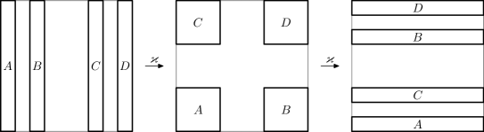
Figure 7. The domain and range of the relation $\varkappa^{2}$ for $M=3$, $\mathcal{A}=\{0,2\}$. See also Figure 1.

The statements (2.31), (2.32) can be interpreted in terms of the canonical relation $\varkappa=\varkappa_{M,\mathcal{A}}$ from (1.3) and the Fourier integral operator $\mathcal{U}_{h}$ from (2.5). Indeed, define the incoming/outgoing tails and the trapped set

$$\Gamma_{\pm}=\bigcap_{\pm r\geq 0}\varkappa^{\,r}\big{(}(0,1)^{2}\big{)},\quad\Gamma=\Gamma_{+}\cap\Gamma_{-}$$ (2.33)

They can be expressed in terms of the Cantor set $\mathcal{C}_{\infty}$ defined in (1.16):

$$\Gamma_{+}=\{x\in(0,1),\ \xi\in\mathcal{C}_{\infty}\},\quad\Gamma_{-}=\{\xi\in(0,1),\ x\in\mathcal{C}_{\infty}\}.$$

See Figure 7. Then (2.32) corresponds to the statement that functions in the range of $\mathcal{U}_{h}^{\tilde{k}}$ (that is, outgoing functions) are microlocalized $h^{\rho}$ close to $\Gamma_{+}$. Similarly (2.31) corresponds to the statement that functions in the range of the adjoint of $\mathcal{U}_{h}^{\tilde{k}}$ (that is, incoming functions) are microlocalized $h^{\rho}$ close to $\Gamma_{-}$.

Applied to eigenfunctions of $B_{N}$, (2.31) and (2.32) give the following statement. (See [DyZa, Lemma 4.6] for its analog in the continuous setting of hyperbolic surfaces.)

Proposition 2.5.

Fix $\nu>0,\rho\in(0,1)$ and assume that for some $k\in\mathbb{N},\lambda\in\mathbb{C},u\in\ell^{2}_{N}$,

$$B_{N}u=\lambda u,\quad|\lambda|\geq M^{-\nu}.$$

Then, with $X_{\rho}$ defined in (2.29),

$$\|u\|_{\ell^{2}_{N}}\leq M^{\nu}|\lambda|^{-\rho k}\,\|\operatorname{1\hskip-2.75ptl}_{X_{\rho}}u\|_{\ell^{2}_{N}}+\mathcal{O}(N^{-\infty})\|u\|_{\ell^{2}_{N}},$$ (2.34)

$$\|u-\mathcal{F}_{N}^{*}\operatorname{1\hskip-2.75ptl}_{X_{\rho}}\mathcal{F}_{N}u\|_{\ell^{2}_{N}}=\mathcal{O}(N^{-\infty})\|u\|_{\ell^{2}_{N}}$$ (2.35)

where the constants in $\mathcal{O}(N^{-\infty})$ depend only on $\nu,\rho,\chi$.

Proof.

Define $\tilde{k}$ by (2.28). Then

$$(B_{N})^{\tilde{k}}u=\lambda^{\tilde{k}}u,\quad|\lambda|^{-\tilde{k}}\leq M^{\nu}N^{\rho\nu}.$$

Applying (2.31) to $\lambda^{-\tilde{k}}u$ and using the bound $\|B_{N}\|_{\ell^{2}_{N}\to\ell^{2}_{N}}\leq 1$, we obtain (2.34). Applying (2.32) to $\lambda^{-\tilde{k}}u$, we obtain (2.35). ∎

Finally, Proposition 2.5 implies the following statement, which proves the second part of Theorem 2.

Proposition 2.6.

With $r_{k}$ defined in (1.10), put

$$\beta:=-\limsup_{k\to\infty}{\log r_{k}\over k\log M}.$$ (2.36)

Then

$$\limsup_{N\to\infty}\max\{|\lambda|\colon\lambda\in\operatorname{Sp}(B_{N})\}\ \leq\ M^{-\beta}.$$ (2.37)

Proof.

Fix $\rho\in(0,1)$. Take $k\in\mathbb{N}$, $N:=M^{k}$, and assume that $\lambda\in\mathbb{C}$ is an eigenvalue of $B_{N}$ such that $|\lambda|\geq M^{-\beta}$. (Note that $\beta$ is always finite, see (3.30).) Choose a normalized eigenfunction

$$u\in\ell^{2}_{N},\quad B_{N}u=\lambda u,\quad\|u\|_{\ell^{2}_{N}}=1.$$

Combining (2.34) and (2.35), we obtain

$$1=\|u\|_{\ell^{2}_{N}} \leq M^{\beta}|\lambda|^{-\rho k}\|\operatorname{1\hskip-2.75ptl}_{X_{\rho}}\mathcal{F}_{N}^{*}\operatorname{1\hskip-2.75ptl}_{X_{\rho}}\mathcal{F}_{N}u\|_{\ell^{2}_{N}}+\mathcal{O}(N^{-\infty})$$ (2.38)

$$\leq M^{\beta}|\lambda|^{-\rho k}\|\operatorname{1\hskip-2.75ptl}_{X_{\rho}}\mathcal{F}_{N}^{*}\operatorname{1\hskip-2.75ptl}_{X_{\rho}}\|_{\ell^{2}_{N}\to\ell^{2}_{N}}+\mathcal{O}(N^{-\infty})$$

where the constants in $\mathcal{O}(N^{-\infty})$ depend only on $\beta,\rho,\chi$.

Using (3.8), the following corollary of (2.29):

$$0\leq\mathbf{1}_{X_{\rho}}\leq\sum_{m\in\mathbb{Z},\,|m|\leq 2N^{1-\rho}}\mathbf{1}_{\mathcal{C}_{k}+m},$$

and the triangle inequality for the operator norm, we estimate

$$\|\operatorname{1\hskip-2.75ptl}_{X_{\rho}}\mathcal{F}_{N}^{*}\operatorname{1\hskip-2.75ptl}_{X_{\rho}}\|_{\ell^{2}_{N}\to\ell^{2}_{N}} =\|\operatorname{1\hskip-2.75ptl}_{X_{\rho}}\mathcal{F}_{N}\operatorname{1\hskip-2.75ptl}_{X_{\rho}}\|_{\ell^{2}_{N}\to\ell^{2}_{N}}$$ (2.39)

$$\leq\sum_{|m|,|m^{\prime}|\leq 2N^{1-\rho}}\|\operatorname{1\hskip-2.75ptl}_{\mathcal{C}_{k}+m}\mathcal{F}_{N}\operatorname{1\hskip-2.75ptl}_{\mathcal{C}_{k}+m^{\prime}}\|_{\ell^{2}_{N}\to\ell^{2}_{N}}$$

$$\leq 5N^{2(1-\rho)}r_{k}.$$

Combining (2.38) and (2.39), we obtain a bound on the spectral radius of $B_{N}$:

$$\big{(}\max\{|\lambda|\colon\lambda\in\operatorname{Sp}(B_{N})\}\big{)}^{\rho k}\leq\max\big{\{}M^{-\beta\rho k},5M^{\beta}N^{2(1-\rho)}r_{k}\big{\}}.$$

Taking both sides to the power $1\over\rho k$ and taking the limit, we get

$$\limsup_{N\to\infty}\max\{|\lambda|\colon\lambda\in\operatorname{Sp}(B_{N})\}\leq\max\{M^{-\beta},M^{(2-2\rho-\beta)/\rho}\}.$$

This is true for all $\rho\in(0,1)$; taking the limit $\rho\to 1$, we obtain (2.37). ∎

3. Fractal uncertainty principle

In this section, we study bounds on the operator norms

$$\|\operatorname{1\hskip-2.75ptl}_{X}\mathcal{F}_{N}\operatorname{1\hskip-2.75ptl}_{Y}\|_{\ell^{2}_{N}\to\ell^{2}_{N}}$$ (3.1)

where $X,Y\subset\mathbb{Z}_{N}$. We will derive several general bounds and apply them to the special case of Cantor sets $\mathcal{C}_{k}$ defined in (1.9), estimating the norm

$$r_{k}:=\|\operatorname{1\hskip-2.75ptl}_{\mathcal{C}_{k}}\mathcal{F}_{N}\operatorname{1\hskip-2.75ptl}_{\mathcal{C}_{k}}\|_{\ell^{2}_{N}\to\ell^{2}_{N}}$$ (3.2)

and finishing the proof of Theorem 2 (see the end of §3.3). We also establish better bounds when $\delta$ is close to $1/2$ using additive energy (see §3.4), consider the special case when the fractal uncertainty principle exponent $\beta$ defined in (1.11) has the maximal possible value (see §3.5), and give lower bounds on $r_{k}$ (see §3.6).

First of all, we have the following basic estimates:

$$\|\operatorname{1\hskip-2.75ptl}_{X}\mathcal{F}_{N}\operatorname{1\hskip-2.75ptl}_{Y}\|_{\ell^{2}_{N}\to\ell^{2}_{N}} \leq 1,$$ (3.3)

$$\|\operatorname{1\hskip-2.75ptl}_{X}\mathcal{F}_{N}\operatorname{1\hskip-2.75ptl}_{Y}\|_{\ell^{2}_{N}\to\ell^{2}_{N}} \leq\sqrt{|X|\cdot|Y|\over N}.$$ (3.4)

The operator norm bound (3.4) follows from the following formula for the Hilbert–Schmidt norm:

$$\|\operatorname{1\hskip-2.75ptl}_{X}\mathcal{F}_{N}\operatorname{1\hskip-2.75ptl}_{Y}\|_{\operatorname{HS}}=\sqrt{|X|\cdot|Y|\over N}.$$ (3.5)

For the case of Cantor sets $X=Y=\mathcal{C}_{k}$, the bounds (3.3), (3.4) yield

$$r_{k}\leq\min\big{(}1,N^{\delta-{1\over 2}}\big{)}$$ (3.6)

where $\delta\in(0,1)$ is defined in (1.5). Therefore, the exponent $\beta$ defined in (1.11) satisfies

$$\beta\geq\max\Big{(}0,{1\over 2}-\delta\Big{)}.$$

(We will show that the limit (1.11) exists in Proposition 3.3 below.) Also, if we define

$$\operatorname{supp}u:=\{j\in\mathbb{Z}_{N}\mid u(j)\neq 0\},\quad u\in\ell^{2}_{N},$$

then (3.1) is equal to

$$\sup\bigg{\{}{|\langle\mathcal{F}_{N}u,v\rangle|\over\|u\|_{\ell^{2}_{N}}\|v\|_{\ell^{2}_{N}}}\colon u,v\in\ell^{2}_{N}\setminus\{0\},\ \operatorname{supp}u\subset Y,\ \operatorname{supp}v\subset X\bigg{\}}.$$ (3.7)

Finally, if $X,Y\subset\mathbb{Z}_{N}$, $j,k\in\mathbb{Z}_{N}$, and the sets $X+j,Y+k$ are defined using addition in $\mathbb{Z}_{N}$, then

$$\|\operatorname{1\hskip-2.75ptl}_{X+j}\mathcal{F}_{N}\operatorname{1\hskip-2.75ptl}_{Y+k}\|_{\ell^{2}_{N}\to\ell^{2}_{N}}=\|\operatorname{1\hskip-2.75ptl}_{X}\mathcal{F}_{N}\operatorname{1\hskip-2.75ptl}_{Y}\|_{\ell^{2}_{N}\to\ell^{2}_{N}}.$$ (3.8)

Indeed, the circular shift gives a unitary operator on $\ell^{2}_{N}$, and it is conjugated by the Fourier transform to a multiplication operator which commutes with $\operatorname{1\hskip-2.75ptl}_{X},\operatorname{1\hskip-2.75ptl}_{Y}$.

In particular (3.8) implies that if $j\geq 1$ and $\mathcal{A}\subset\{0,\dots,M-j-1\}$, then the pairs $(M,\mathcal{A})$ and $(M,\mathcal{A}+j)$ have the same norms $r_{k}$, and thus the same value of $\beta$ defined in (1.11).

3.1. Submultiplicativity

In this section, we assume that $N$ factorizes as $N=N_{1}N_{2}$, where $N_{1},N_{2}\in\mathbb{N}$. The following lemma gives a way to reduce the Fourier transform $\mathcal{F}_{N}$ to Fourier transforms $\mathcal{F}_{N_{1}},\mathcal{F}_{N_{2}}$, using a technique similar to the one employed in fast Fourier transform (FFT) algorithms. The resulting submultiplicative inequality (3.10) is a crucial component of the proof of Theorem 2, making it possible to reduce bounds for large $N$ to bounds for bounded $N$.

Lemma 3.1.

Assume $u,v\in\ell^{2}_{N}$. For $\ell_{1},j_{2}\in\mathbb{Z}_{N}$, define $\tilde{u}_{\ell_{1}}\in\ell^{2}_{N_{2}}$, $\tilde{v}_{j_{2}}\in\ell^{2}_{N_{1}}$ by

$$\tilde{u}_{\ell_{1}}(\ell_{2})=u(\ell_{1}+N_{1}\ell_{2}), \quad\ell_{2}\in\mathbb{Z}_{N_{2}};$$

$$\tilde{v}_{j_{2}}(j_{1})=v(j_{2}+N_{2}j_{1}), \quad j_{1}\in\mathbb{Z}_{N_{1}}.$$

Then

$$\langle\mathcal{F}_{N}u,v\rangle=\sum_{\ell_{1}=0}^{N_{1}-1}\sum_{j_{2}=0}^{N_{2}-1}\exp\Big{(}-{2\pi ij_{2}\ell_{1}\over N}\Big{)}\mathcal{F}_{N_{2}}\tilde{u}_{\ell_{1}}(j_{2})\cdot\overline{\mathcal{F}_{N_{1}}^{*}\tilde{v}_{j_{2}}(\ell_{1})}.$$ (3.9)

Proof.

We write

$$\langle\mathcal{F}_{N}u,v\rangle ={1\over\sqrt{N}}\sum_{j,\ell=0}^{N-1}\exp\Big{(}-{2\pi ij\ell\over N}\Big{)}u(\ell)\overline{v(j)}$$

$$={1\over\sqrt{N}}\sum_{j_{1},\ell_{1}=0}^{N_{1}-1}\sum_{j_{2},\ell_{2}=0}^{N_{2}-1}\exp\Big{(}-{2\pi i(j_{2}+N_{2}j_{1})(\ell_{1}+N_{1}\ell_{2})\over N}\Big{)}\tilde{u}_{\ell_{1}}(\ell_{2})\overline{\tilde{v}_{j_{2}}(j_{1})}.$$

Now, since $\exp(-2\pi ij_{1}\ell_{2})=1$, we have for each $j_{2},\ell_{1}$

$$\begin{gathered}{1\over\sqrt{N}}\sum_{j_{1}=0}^{N_{1}-1}\sum_{\ell_{2}=0}^{N_{2}-1}\exp\Big{(}-{2\pi i(j_{2}+N_{2}j_{1})(\ell_{1}+N_{1}\ell_{2})\over N}\Big{)}\tilde{u}_{\ell_{1}}(\ell_{2})\overline{\tilde{v}_{j_{2}}(j_{1})}\\ =\exp\Big{(}-{2\pi ij_{2}\ell_{1}\over N}\Big{)}\mathcal{F}_{N_{2}}\tilde{u}_{\ell_{1}}(j_{2})\cdot\overline{\mathcal{F}_{N}^{*}\tilde{v}_{j_{2}}(\ell_{1})}\end{gathered}$$

finishing the proof. ∎

As a corollary of Lemma 3.1 we get the following bound on the norm (3.1) when the sets $X,Y$ have special structure:

Lemma 3.2.

Assume that $X_{1},Y_{1}\subset\{0,\dots,N_{1}-1\}$, $X_{2},Y_{2}\subset\{0,\dots,N_{2}-1\}$, and define $X,Y\subset\{0,\dots,N-1\}\simeq\ell^{2}_{N}$ by

$$X :=\{j_{2}+N_{2}j_{1}\mid j_{1}\in X_{1},\ j_{2}\in X_{2}\},$$

$$Y :=\{\ell_{1}+N_{1}\ell_{2}\mid\ell_{1}\in Y_{1},\ \ell_{2}\in Y_{2}\}.$$

Then

$$\|\operatorname{1\hskip-2.75ptl}_{X}\mathcal{F}_{N}\operatorname{1\hskip-2.75ptl}_{Y}\|_{\ell^{2}_{N}\to\ell^{2}_{N}}\leq\|\operatorname{1\hskip-2.75ptl}_{X_{1}}\mathcal{F}_{N_{1}}\operatorname{1\hskip-2.75ptl}_{Y_{1}}\|_{\ell^{2}_{N_{1}}\to\ell^{2}_{N_{1}}}\cdot\|\operatorname{1\hskip-2.75ptl}_{X_{2}}\mathcal{F}_{N_{2}}\operatorname{1\hskip-2.75ptl}_{Y_{2}}\|_{\ell^{2}_{N_{2}}\to\ell^{2}_{N_{2}}}.$$

Proof.

We use (3.7). Assume that $u,v\in\ell^{2}_{N}$ and $\operatorname{supp}u\subset Y$, $\operatorname{supp}v\subset X$. To estimate $\langle\mathcal{F}_{N}u,v\rangle$, we use (3.9). We have $\tilde{u}_{\ell_{1}}=0$ unless $\ell_{1}\in Y_{1}$, and $\tilde{v}_{j_{2}}=0$ unless $j_{2}\in X_{2}$, therefore the sum on the right-hand side of (3.9) can be taken over $\ell_{1}\in Y_{1},j_{2}\in X_{2}$. By Cauchy–Schwartz, we then get

$$|\langle\mathcal{F}_{N}u,v\rangle|^{2}\leq\bigg{(}\sum_{\ell_{1}\in Y_{1}\atop j_{2}\in X_{2}}|\mathcal{F}_{N_{2}}\tilde{u}_{\ell_{1}}(j_{2})|^{2}\bigg{)}\bigg{(}\sum_{\ell_{1}\in Y_{1}\atop j_{2}\in X_{2}}|\mathcal{F}_{N_{1}}^{*}\tilde{v}_{j_{2}}(\ell_{1})|^{2}\bigg{)}.$$

Since $\operatorname{supp}\tilde{u}_{\ell_{1}}\subset Y_{2}$, $\operatorname{supp}\tilde{v}_{j_{2}}\subset X_{1}$, we have

$$\sum_{\ell_{1}\in Y_{1}\atop j_{2}\in X_{2}}|\mathcal{F}_{N_{2}}\tilde{u}_{\ell_{1}}(j_{2})|^{2} \leq\ \|\operatorname{1\hskip-2.75ptl}_{X_{2}}\mathcal{F}_{N_{2}}\operatorname{1\hskip-2.75ptl}_{Y_{2}}\|_{\ell^{2}_{N_{2}}\to\ell^{2}_{N_{2}}}^{2}\cdot\|u\|_{\ell^{2}_{N}}^{2},$$

$$\sum_{\ell_{1}\in Y_{1}\atop j_{2}\in X_{2}}|\mathcal{F}_{N_{1}}^{*}\tilde{v}_{j_{2}}(\ell_{1})|^{2} \leq\ \|\operatorname{1\hskip-2.75ptl}_{Y_{1}}\mathcal{F}_{N_{1}}^{*}\operatorname{1\hskip-2.75ptl}_{X_{1}}\|_{\ell^{2}_{N_{1}}\to\ell^{2}_{N_{1}}}^{2}\cdot\|v\|_{\ell^{2}_{N}}^{2}$$

finishing the proof. ∎

In the case of Cantor sets (1.9), by putting $N_{1}=M^{k_{1}},N_{2}=M^{k_{2}}$, $X_{1}=Y_{1}=\mathcal{C}_{k_{1}}$, $X_{2}=Y_{2}=\mathcal{C}_{k_{2}}$, $X=Y=\mathcal{C}_{k}$, Lemma 3.2 implies the following submultiplicative inequality on the norm $r_{k}$ defined in (3.2):

$$r_{k_{1}+k_{2}}\leq r_{k_{1}}r_{k_{2}},\quad k_{1},k_{2}\in\mathbb{N}.$$ (3.10)

The sequence $\log r_{k}$ is then subadditive, which by Fekete’s Lemma gives

Proposition 3.3.

For $\beta$ defined in (2.36), we have

$$\beta=-\lim_{k\to\infty}{\log r_{k}\over k\log M}=-\inf_{k}{\log r_{k}\over k\log M}.$$ (3.11)

Proposition 3.3 implies that the inequality in (1.11) is proven once we show that

$$-{\log r_{k}\over k\log M}>\max\Big{(}0,{1\over 2}-\delta\Big{)}\quad\text{for some }k.$$ (3.12)

3.2. Improvements over the pressure bound

We start the proof of (3.12) by improving over the pressure bound ${1\over 2}-\delta$. We rely on the following general

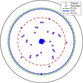
Figure 8. The spectrum of $B_{N}$ for $M=6$, $\mathcal{A}=\{2,3\}$, $k=5$. The pressure bound on the spectral radius is not sharp but the slightly smaller fractal uncertainty bound appears to be sharp.

Lemma 3.4.

Assume $X,Y\subset\mathbb{Z}_{N}$ and there exist

$$j,j^{\prime}\in X,\quad\ell,\ell^{\prime}\in Y,\quad(j-j^{\prime})(\ell-\ell^{\prime})\notin N\mathbb{Z}.$$ (3.13)

Then for some global constant $\mathbf{K}$,

$$\|\operatorname{1\hskip-2.75ptl}_{X}\mathcal{F}_{N}\operatorname{1\hskip-2.75ptl}_{Y}\|_{\ell^{2}_{N}\to\ell^{2}_{N}}\leq\Big{(}1-{1\over\mathbf{K}N^{4}}\Big{)}\sqrt{|X|\cdot|Y|\over N}.$$ (3.14)

Proof.

Let $\sigma_{1}\geq\sigma_{2}\geq\dots\sigma_{N}\geq 0$ be the singular values of $\operatorname{1\hskip-2.75ptl}_{X}\mathcal{F}_{N}\operatorname{1\hskip-2.75ptl}_{Y}$. Then

$$\sigma_{1}=\|\operatorname{1\hskip-2.75ptl}_{X}\mathcal{F}_{N}\operatorname{1\hskip-2.75ptl}_{Y}\|_{\ell^{2}_{N}\to\ell^{2}_{N}}.$$

Moreover, by (3.5)

$$\sigma_{1}^{2}+\sigma_{2}^{2}\leq\sum_{r=1}^{N}\sigma_{r}^{2}=\|\operatorname{1\hskip-2.75ptl}_{X}\mathcal{F}_{N}\operatorname{1\hskip-2.75ptl}_{Y}\|_{\operatorname{HS}}^{2}={|X|\cdot|Y|\over N}.$$ (3.15)

It then remains to obtain a lower bound on $\sigma_{1}\sigma_{2}$.

By Weyl inequalities for products of operators [HoJo, Theorem 3.3.16(d)], the singular values of $\operatorname{1\hskip-2.75ptl}_{X}\mathcal{F}_{N}\operatorname{1\hskip-2.75ptl}_{Y}$ are greater than or equal than those of

$$\operatorname{1\hskip-2.75ptl}_{X^{\prime}}\mathcal{F}_{N}\operatorname{1\hskip-2.75ptl}_{Y^{\prime}}=\operatorname{1\hskip-2.75ptl}_{X^{\prime}}(\operatorname{1\hskip-2.75ptl}_{X}\mathcal{F}_{N}\operatorname{1\hskip-2.75ptl}_{Y})\operatorname{1\hskip-2.75ptl}_{Y^{\prime}},\quad X^{\prime}:=\{j,j^{\prime}\},\quad Y^{\prime}:=\{\ell,\ell^{\prime}\}.$$ (3.16)

The matrix of (3.16) only has four nonzero elements, and the absolute value of the determinant of the $2\times 2$ matrix composed of these is equal to

$${2\over N}\Big{|}\sin\Big{(}{\pi\over N}(j-j^{\prime})(\ell-\ell^{\prime})\Big{)}\Big{|}\geq{2\over N}\sin\Big{(}{\pi\over N}\Big{)}$$

where in the last inequality we used (3.13). Therefore,

$$\sigma_{1}\sigma_{2}\geq{2\over N}\sin\Big{(}{\pi\over N}\Big{)}$$

and by (3.15) we have for $|X|\cdot|Y|\leq N$ and some global constant $\mathbf{K}$,

$$\sigma_{1}^{2} ={\sigma_{1}^{2}+\sigma_{2}^{2}+\sqrt{(\sigma_{1}^{2}+\sigma_{2}^{2})^{2}-4\sigma_{1}^{2}\sigma_{2}^{2}}\over 2}$$

$$\leq{|X|\cdot|Y|\over 2N}\Bigg{(}1+\sqrt{1-{16\over|X|^{2}\cdot|Y|^{2}}\sin^{2}\Big{(}{\pi\over N}\Big{)}}\,\Bigg{)}$$

$$\leq{|X|\cdot|Y|\over N}\Big{(}1-{1\over\mathbf{K}N^{4}}\Big{)}^{2}.$$

For $|X|\cdot|Y|\geq N+1$, (3.14) holds simply by (3.3); this finishes the proof. ∎

In the case of Cantor sets, Lemma 3.4 implies

Corollary 3.5.

We have for some global constant $\mathbf{K}$ and $\beta$ defined in (3.11)

$$\beta\geq-{\log r_{2}\over 2\log M}\geq{1\over 2}-\delta+{1\over\mathbf{K}M^{8}\log M}.$$ (3.17)

Proof.

Take $a,a^{\prime}\in\mathcal{A}$, $a<a^{\prime}$, and put $j=\ell=Ma+a$, $j^{\prime}=\ell^{\prime}=Ma+a^{\prime}$. Then $(j-j^{\prime})(\ell-\ell^{\prime})=(a^{\prime}-a)^{2}\in(0,M^{2})$, thus (3.13) holds for $N=M^{2}$, $X=Y=\mathcal{C}_{2}$. The bound (3.14) then gives (3.17). ∎

Remark. The power of $M$ in (3.17) is most likely not sharp. However, Proposition 3.17 below gives examples of alphabets for $\delta<1/2$ with a power upper bound on the improvement $\beta-({1\over 2}-\delta)$. See Table 1 and Figure 8 for numerical evidence.

$M$	$|\mathcal{A}|$	$\delta$	$k$	$\beta_{\min}-\max(0,{1\over 2}-\delta)$	$M$	$|\mathcal{A}|$	$\delta$	$k$	$\beta_{\min}-\max(0,{1\over 2}-\delta)$
10	2	0.3010	12	$5.4\cdot 10^{-3}$	9	2	0.3155	12	$6.5\cdot 10^{-3}$
8	2	0.3333	12	$9.5\cdot 10^{-3}$	7	2	0.3562	12	$1.3\cdot 10^{-2}$
6	2	0.3869	12	$2\cdot 10^{-2}$	5	2	0.4307	12	$3.2\cdot 10^{-2}$
10	3	0.4771	7	$3.7\cdot 10^{-2}$	4	2	0.5000	12	$\mathbf{5.4\cdot 10^{-2}}$
9	3	0.5000	7	$\mathbf{4.1\cdot 10^{-2}}$	8	3	0.5283	7	$3.4\cdot 10^{-2}$
7	3	0.5646	7	$2.1\cdot 10^{-2}$	10	4	0.6021	6	$7.3\cdot 10^{-3}$
6	3	0.6131	7	$8.7\cdot 10^{-3}$	3	2	0.6309	12	$6.2\cdot 10^{-3}$
9	4	0.6309	6	$3.6\cdot 10^{-3}$	8	4	0.6667	6	$1.1\cdot 10^{-3}$
5	3	0.6826	7	$5.1\cdot 10^{-4}$	10	5	0.6990	5	$1.3\cdot 10^{-4}$
7	4	0.7124	6	$4.8\cdot 10^{-5}$	9	5	0.7325	5	$4.6\cdot 10^{-6}$
6	4	0.7737	6	$3.5\cdot 10^{-7}$	8	5	0.7740	5	$4.5\cdot 10^{-8}$
10	6	0.7782	4	$4.1\cdot 10^{-9}$	4	3	0.7925	7	$3\cdot 10^{-7}$
9	6	0.8155	4	$<10^{-12}$	7	5	0.8271	5	$1.9\cdot 10^{-11}$
10	7	0.8451	4	$<10^{-12}$	5	4	0.8614	6	$<10^{-12}$
8	6	0.8617	4	$<10^{-12}$	9	7	0.8856	4	$<10^{-12}$
6	5	0.8982	5	$<10^{-12}$	10	8	0.9031	4	$<10^{-12}$
7	6	0.9208	4	$<10^{-12}$	8	7	0.9358	4	$<10^{-12}$
9	8	0.9464	4	$<10^{-12}$	10	9	0.9542	3	$<10^{-12}$

Table 1. Numerically computed minimal values $\beta_{\min}$ of $-\log r_{k}/(k\log M)$ (which approximate the fractal uncertainty exponents $\beta(M,\mathcal{A})$ by (3.11)) for fixed $M,|\mathcal{A}|$, sorted by $\delta$. The alphabets achieving $\beta_{\min}$ were all arithmetic progressions, mostly with difference $1$. Note that the improvement over the standard bound, $\beta_{\min}-\max(0,{1\over 2}-\delta)$, is the largest when $\delta={1\over 2}$, and is very small when $\delta$ is close to 1, already for $M=4$. This is in agreement with the lower envelope of Figure 3.

3.3. Improvements over the zero bound

We next show that the left-hand side of (3.12) is greater than 0 for some $k$. We rely on the following general

Lemma 3.6.

Assume $X,Y\subset\mathbb{Z}_{N}$ and for some $L\in\{1,\dots,N-1\}$, the following two conditions hold:

1. $|X|\leq L$;

2. $Y$ has a gap of size $L$, that is there exists $j\in\mathbb{Z}_{N}$ such that $j,\dots,j+L-1\notin Y$, with addition carried in $\mathbb{Z}_{N}$.

Then

$$\|\operatorname{1\hskip-2.75ptl}_{X}\mathcal{F}_{N}\operatorname{1\hskip-2.75ptl}_{Y}\|_{\ell^{2}_{N}\to\ell^{2}_{N}}\leq\sqrt{1-2^{-2N}}.$$ (3.18)

Proof.

By cyclically shifting $Y$ and using (3.8) we may assume that

$$Y\subset\{0,\dots,N-L-1\}.$$

Assume that $u\in\ell^{2}_{N}$, $\|u\|_{\ell^{2}_{N}}=1$, $\operatorname{supp}u\subset Y$, and consider the polynomial

$$p(z)=\sum_{\ell\in Y}u(\ell)z^{\ell}.$$

Note that $p$ has degree at most $N-L-1$. Denoting $\omega_{N}=\exp(-2\pi i/N)$, we have

$$\mathcal{F}_{N}u(j)={1\over\sqrt{N}}\,p(\omega_{N}^{j}),\quad j\in\mathbb{Z}_{N}.$$

Using that $\|\mathcal{F}_{N}u\|_{\ell^{2}_{N}}=1$, we compute

$$\|\operatorname{1\hskip-2.75ptl}_{X}\mathcal{F}_{N}u\|_{\ell^{2}_{N}}^{2}=1-{1\over N}\sum_{0\leq j<N\atop j\notin X}|p(\omega_{N}^{j})|^{2}.$$

This immediately shows that $\|\operatorname{1\hskip-2.75ptl}_{X}\mathcal{F}_{N}u\|_{\ell^{2}_{N}}<1$, since otherwise the equation $p(z)=0$ has at least $N-|X|\geq N-L$ roots.

To get a quantitative bound, we use Lagrange interpolation: since $p$ has degree at most $N-L-1<N-|X|$, we write

$$p(z)=\sum_{0\leq j<N\atop j\notin X}p(\omega_{N}^{j})\mathcal{L}_{j}(z),\quad\mathcal{L}_{j}(z)=\prod_{0\leq m<N\atop m\notin X,\ m\neq j}{z-\omega_{N}^{m}\over\omega_{N}^{j}-\omega_{N}^{m}}.$$

Differentiating at $z=1$ the polynomial

$$z^{N}-1=\prod_{r=0}^{N-1}(z-\omega_{N}^{r}),$$

we get for each $j\in\mathbb{Z}_{N}$

$$N=\prod_{r=1}^{N-1}(1-\omega_{N}^{r})=\prod_{0\leq m<N\atop m\neq j}|\omega_{N}^{j}-\omega_{N}^{m}|.$$

Assume $|z|=1$; since $|z-\omega_{N}^{r}|\leq 2$, we get for $j\notin X$

$$|\mathcal{L}_{j}(z)|\leq{2^{N-|X|}\over N}\prod_{m\in X}|\omega_{N}^{j}-\omega_{N}^{m}|\leq{2^{N}\over N}.$$

Therefore, by Hölder’s inequality we have for $|z|=1$

$$|p(z)|^{2}\leq{2^{2N}\over N}\sum_{0\leq j<N\atop j\notin X}|p(\omega_{N}^{j})|^{2}=2^{2N}\big{(}1-\|\operatorname{1\hskip-2.75ptl}_{X}\mathcal{F}_{N}u\|_{\ell^{2}_{N}}^{2}\big{)}.$$

Since

$$1=\|\mathcal{F}_{N}u\|_{\ell^{2}_{N}}^{2}={1\over N}\sum_{r=0}^{N}|p(\omega_{N}^{r})|^{2},$$

we obtain $\|\operatorname{1\hskip-2.75ptl}_{X}\mathcal{F}_{N}u\|_{\ell^{2}_{N}}^{2}\leq 1-2^{-2N}$, finishing the proof. ∎

In the case of Cantor sets, Lemma 3.6 implies

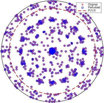
Figure 9. The spectrum of $B_{N}$ for $M=7$, $\mathcal{A}=\{1,2,3,4,5\}$, $k=4$. The numerically computed uncertainty principle exponent is $\sim 10^{-11}$ and the spectral radius appears to be very close to 1.

Corollary 3.7.

For $\beta$ defined in (3.11), we have

$$\beta\geq-{\log r_{k}\over k\log M}\geq{2^{-2M^{k}}\over 2k\log M}>0\quad\text{for all }k\geq{1\over 1-\delta}-{\log\lceil M^{1-\delta}-1\rceil\over(1-\delta)\log M}.$$ (3.19)

Proof.

For each $a\in\mathcal{A}$, define

$$L_{a}:=\max\{j\geq 0\colon a+\ell\notin\mathcal{A}\text{ for all }\ell\in\mathbb{Z},\ 1\leq\ell\leq j\}$$

where addition is carried in $\mathbb{Z}_{M}$. We have

$$\sum_{a\in\mathcal{A}}(L_{a}+1)=M.$$

Therefore, there exists $a\in\mathcal{A}$ such that $L_{a}\geq\lceil M^{1-\delta}-1\rceil$. Then the set $\mathcal{C}_{k}$ has a gap starting at $(a+1)M^{k-1}$ of size

$$L=\lceil M^{1-\delta}-1\rceil M^{k-1}.$$

By the condition on $k$, we have

$$|\mathcal{C}_{k}|=M^{\delta k}\leq L.$$

Applying Lemma 3.6 with $N=M^{k}$, $X=Y=\mathcal{C}_{k}$, we obtain (3.19). ∎

Remark. For fixed $\delta\in(0,1)$ and large $M$, the bound on $k$ in (3.19) is asymptotic to $k\geq\delta/(1-\delta)$. While we prove no upper bounds on $\beta$, numerical evidence in Table 1 and Figure 9 suggests that there exists some alphabets with $\delta>{1\over 2}$ for which $\beta$ is very small and the spectral radius of $B_{N}$ is very close to 1.

We are now ready to finish the

Proof of Theorem 2.

The existence of the limit in (1.11) follows from Proposition 3.3. The fact that $\beta>\max(0,{1\over 2}-\delta)$ follows from Corollaries 3.5 and 3.7. Finally the asymptotic spectral radius bound (1.8) follows from Proposition 2.6. ∎

3.4. Improvements using additive energy

So far we have established lower bounds on the improvement $\beta-\max(0,{1\over 2}-\delta)$, with $\beta$ defined in (3.11), which decay like a power of $M$ for $\delta\leq{1\over 2}$ (see Corollary 3.5) and exponentially in $M$ for $\delta\geq{1\over 2}$ (see Corollary 3.7). However, Figure 3 and Table 1 indicate that the value of $\beta-\max(0,{1\over 2}-\delta)$ should be larger when $\delta\approx{1\over 2}$. In this section we explain this observation by establishing lower bounds on $\beta$ which decay like ${1\over\log M}$ when $\delta\approx{1\over 2}$.

Our bounds rely on the following general statement:

Lemma 3.8.

Assume $X,Y\subset\mathbb{Z}_{N}$. Then

$$\|\operatorname{1\hskip-2.75ptl}_{X}\mathcal{F}_{N}\operatorname{1\hskip-2.75ptl}_{Y}\|_{\ell^{2}_{N}\to\ell^{2}_{N}}\leq{\widetilde{E}_{A}(X)^{1/8}|Y|^{3/8}\over N^{3/8}}$$

where the quantity $\widetilde{E}_{A}(X)$, called additive energy of $X$, is defined by

$$\widetilde{E}_{A}(X):=\big{|}\{(a,b,c,d)\in X^{4}\mid a+b=c+d\mod N\}\big{|}.$$

Proof.

The operator $A=(\operatorname{1\hskip-2.75ptl}_{X}\mathcal{F}_{N}\operatorname{1\hskip-2.75ptl}_{Y})^{*}\operatorname{1\hskip-2.75ptl}_{X}\mathcal{F}_{N}\operatorname{1\hskip-2.75ptl}_{Y}=\operatorname{1\hskip-2.75ptl}_{Y}\mathcal{F}_{N}^{*}\operatorname{1\hskip-2.75ptl}_{X}\mathcal{F}_{N}\operatorname{1\hskip-2.75ptl}_{Y}$ has the matrix

$$A_{j\ell}={\mathbf{1}_{Y}(j)\mathbf{1}_{Y}(\ell)\over\sqrt{N}}\mathcal{F}_{N}(\mathbf{1}_{X})(\ell-j)$$

where $\mathbf{1}_{X},\mathbf{1}_{Y}$ denote indicator functions. By Schur’s and Hölder’s inequalities,

$$\|\operatorname{1\hskip-2.75ptl}_{X}\mathcal{F}_{N}\operatorname{1\hskip-2.75ptl}_{Y}\|_{\ell^{2}_{N}\to\ell^{2}_{N}}^{2} =\|A\|_{\ell^{2}_{N}\to\ell^{2}_{N}}$$

$$\leq\max_{j\in Y}\sum_{\ell\in Y}{|\mathcal{F}_{N}(\mathbf{1}_{X})(\ell-j)|\over\sqrt{N}}$$

$$\leq{|Y|^{3/4}\cdot\|\mathcal{F}_{N}(\mathbf{1}_{X})\|_{\ell^{4}_{N}}\over\sqrt{N}}.$$

Now

$$\|\mathcal{F}_{N}(\mathbf{1}_{X})\|_{\ell^{4}_{N}}^{4}={1\over N^{2}}\sum_{\ell=0}^{N-1}\sum_{a,b,c,d\in X}\exp\Big{(}{2\pi i(a+b-c-d)\ell\over N}\Big{)}={\widetilde{E}_{A}(X)\over N}$$

finishing the proof. ∎

We remark that for all $X$

$$|X|^{2}\leq\widetilde{E}_{A}(X)\leq|X|^{3},$$ (3.20)

where the first bound comes from considering quadruples of the form $(a,b,a,b)$ and the second one, from the fact that $a,b,c$ determine $d$. Moreover, by writing

$$\widetilde{E}_{A}(X)=\sum_{j=0}^{N-1}\widetilde{F}_{j}(X)^{2},\quad\widetilde{F}_{j}(X):=\big{|}\{(a,b)\in X^{2}\mid a-b=j\mod N\}\big{|},$$

and using Hölder’s inequality together with the identity $\sum_{j}\widetilde{F}_{j}(X)=|X|^{2}$, we get

$$\widetilde{E}_{A}(X)\geq{|X|^{4}\over N}.$$ (3.21)

In the case of Cantor sets defined in (1.9), Lemma 3.8 immediately gives

Corollary 3.9.

Assume that for some constants $C,\gamma\geq 0$ and all $k$,

$$\widetilde{E}_{A}(\mathcal{C}_{k})\leq CN^{3\delta-\gamma}.$$ (3.22)

Then the exponent $\beta$ defined in (3.11) satisfies

$$\beta\geq{3\over 4}\Big{(}{1\over 2}-\delta\Big{)}+{\gamma\over 8}.$$ (3.23)

Note that by (3.20), (3.21) we have

$$\gamma\leq\min(\delta,1-\delta).$$

Therefore, the bound (3.23) cannot improve over the standard bound $\max(0,{1\over 2}-\delta)$ unless $\delta$ is close to $1/2$, specifically $\delta\in(1/3,4/7)$. However, the advantage of (3.23) over the bounds in Corollaries 3.5, 3.7 for $\delta\approx{1\over 2}$ is that the exponent $\gamma$ from (3.22) can be computed explicitly as follows:

Lemma 3.10.

Let $\rho(\mathcal{A})$ be the spectral radius of the $2\times 2$ matrix

$$\mathcal{M}(\mathcal{A})=\begin{pmatrix}E_{M-1}(\mathcal{A})+E_{M+1}(\mathcal{A})&2E_{M}(\mathcal{A})\\ E_{1}(\mathcal{A})&E_{0}(\mathcal{A})\end{pmatrix}$$ (3.24)

where (with the equality below in $\mathbb{Z}$ rather than $\mathbb{Z}/N\mathbb{Z}$)

$$E_{\ell}(\mathcal{A}):=\big{|}\{(a,b,c,d)\in\mathcal{A}^{4}\mid a+b-c-d=\ell\}\big{|},\quad\ell\in\mathbb{Z}.$$ (3.25)

Then (3.22) holds for each $\gamma<\gamma_{\mathcal{A}}$ where

$$\gamma_{\mathcal{A}}=3\delta-{\log\rho(\mathcal{A})\over\log M}.$$ (3.26)

Proof.

We use the standard addition algorithm, keeping track of the carry digits. For $k\in\mathbb{N}$, consider the vector

$$x^{(k)}=(x^{(k)}_{0},x^{(k)}_{1},x^{(k)}_{2})\in\mathbb{N}_{0}^{3}$$

defined as follows: $x^{(k)}_{j}$ is the number of quadruples $(a,b,c,d)\in\mathcal{C}_{k}^{4}$ such that

$$a+b=c+d+(j-1)M^{k}\quad\text{in }\mathbb{Z}.$$

A direct calculation shows that if we put $x^{(0)}:=(0,1,0)$, then for $k\in\mathbb{N}$

$$x^{(k)}=\begin{pmatrix}E_{M-1}(\mathcal{A})&E_{M}(\mathcal{A})&E_{M+1}(\mathcal{A})\\ E_{1}(\mathcal{A})&E_{0}(\mathcal{A})&E_{1}(\mathcal{A})\\ E_{M+1}(\mathcal{A})&E_{M}(\mathcal{A})&E_{M-1}(\mathcal{A})\end{pmatrix}x^{(k-1)},\quad\widetilde{E}_{A}(\mathcal{C}_{k})=\langle x^{(k)},(1,1,1)\rangle.$$

Now, it is easy to see that $x^{(k)}_{0}=x^{(k)}_{2}$ for all $k$. In fact, if $y^{(k)}=(2x^{(k)}_{0},x^{(k)}_{1})$, then

$$y^{(k)}=\mathcal{M}(\mathcal{A})^{k}\begin{pmatrix}0\\ 1\end{pmatrix},\quad\widetilde{E}_{A}(\mathcal{C}_{k})=\langle y^{(k)},(1,1)\rangle.$$

It follows that (3.22) holds for each $\gamma<\gamma_{A}$. ∎

The next statement, proved in Appendix A, gives a positive lower bound on the exponent $\gamma_{A}$ from (3.26):

Proposition 3.11.

For any $\zeta>0$, there exists a constant $\varepsilon>0$ only depending on $\zeta$ such that whenever $1<|\mathcal{A}|<\frac{2}{3}(1-\zeta)M$, the spectral radius $\rho(\mathcal{A})$ of the matrix $\mathcal{M}(\mathcal{A})$ defined in (3.24) satisfies

$$\rho(\mathcal{A})\leq(1-\varepsilon)|\mathcal{A}|^{3}.$$ (3.27)

Thus $\gamma_{\mathcal{A}}\geq c/\log M$ where $c=-\log(1-\varepsilon)>0$.

Combining Corollary 3.9, Lemma 3.10, and Proposition 3.11, we obtain

Proposition 3.12.

There exists a global constant $\mathbf{K}$ such that for all $(M,\mathcal{A})$ satisfying

$$\Big{|}\delta-{1\over 2}\Big{|}\leq{1\over\mathbf{K}\log M}$$

the fractal uncertainty exponent $\beta=\beta(M,\mathcal{A})$ defined in (3.11) satisfies

$$\beta\geq\max\Big{(}0,{1\over 2}-\delta\Big{)}+{1\over\mathbf{K}\log M}.$$ (3.28)

A family of alphabets with an upper bound on $\beta$ matching (3.28) is presented in Proposition 3.17 below.

3.5. Special alphabets with the best possible exponent

For any two nonempty sets $X,Y\subset\mathbb{Z}_{N}$, we have the lower bound

$$\|\operatorname{1\hskip-2.75ptl}_{X}\mathcal{F}_{N}\operatorname{1\hskip-2.75ptl}_{Y}\|_{\ell^{2}_{N}\to\ell^{2}_{N}}\geq\sqrt{\max(|X|,|Y|)\over N}.$$ (3.29)

Indeed, to show the lower bound of $\sqrt{|X|/N}$, it is enough to apply the operator $\operatorname{1\hskip-2.75ptl}_{X}\mathcal{F}_{N}$ to any element of $\ell^{2}_{N}$ supported at one point of $Y$; taking adjoints, we obtain the lower bound $\sqrt{|Y|/N}$.

For $X=Y=\mathcal{C}_{k}$ defined in (1.9), and $r_{k}$ defined in (3.2), (3.29) gives $r_{k}\geq N^{(\delta-1)/2}$, implying the following bound on the exponent $\beta$ from (3.11):

$$\beta\leq{1-\delta\over 2}.$$ (3.30)

As expected from the numerical evidence in Figure 3 and Table 1, and proved in Proposition 3.16 below, for many alphabets the actual value of $\beta$ is strictly below the upper bound (3.30). However, the next statement implies that there exist alphabets for which (3.30) is an equality, that is $\beta$ takes its largest allowed value:

Proposition 3.13.

For an alphabet $\mathcal{A}\subset\mathbb{Z}_{M}$, define the 1-periodic function

$$G_{\mathcal{A}}(x)={1\over\sqrt{M}}\sum_{a\in\mathcal{A}}\exp(-2\pi iax),\ x\in\mathbb{R}.$$ (3.31)

Assume that

$$G_{\mathcal{A}}\Big{(}{b-b^{\prime}\over M}\Big{)}=0\quad\text{for all }b,b^{\prime}\in\mathcal{A},\ b\neq b^{\prime}.$$ (3.32)

Then

$$r_{k}=\Big{(}{|\mathcal{A}|\over M}\Big{)}^{k/2}\quad\text{for all }k$$ (3.33)

and thus $\beta=(1-\delta)/2$.

Proof.

Condition (3.32) implies that any two different rows of the matrix of the transformation $\operatorname{1\hskip-2.75ptl}_{A}\mathcal{F}_{M}\operatorname{1\hskip-2.75ptl}_{A}$ are orthogonal to each other. Since each of these rows has $\ell^{2}_{M}$ norm equal to 0 or $\sqrt{|\mathcal{A}|/M}$, we have

$$r_{1}=\sqrt{|\mathcal{A}|/M}.$$

By (3.10) we obtain an upper bound on $r_{k}$ which matches the lower bound following from (3.29). This immediately implies (3.33). ∎

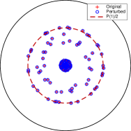
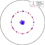
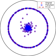
 $M=6$, $\mathcal{A}=\{1,4\}$  $M=8$, $\mathcal{A}=\{2,4\}$ $M=8$, $\mathcal{A}=\{1,2,5,6\}$

Figure 10. The spectra of $B_{N}$ for three alphabets satisfying (3.32), with $k=5$ for $M=6$ and $k=4$ for $M=8$. Each case exhibits a band structure consistent with Conjecture 3.14, in particular the number of the eigenvalues near the outer circle is exactly $|\mathcal{A}|^{k}$.

The alphabets satisfying (3.32) are interesting in particular because all nonzero singular values of the matrix $\operatorname{1\hskip-2.75ptl}_{\mathcal{C}_{k}}\mathcal{F}_{N}\operatorname{1\hskip-2.75ptl}_{\mathcal{C}_{k}}$ are equal to $(|\mathcal{A}|/M)^{k/2}$, as follows from (3.5). Therefore we expect that as long as $0,M-1\notin\mathcal{A}$ and the cutoff $\chi$ is equal to 1 near the Cantor set $\mathcal{C}_{\infty}$ (see Theorem 4), many eigenvalues of the open quantum map $B_{N,\chi}$ will lie near the circle of radius $\sqrt{|\mathcal{A}|/M}$. Indeed, if an eigenfunction $u$ with eigenvalue $\lambda$ satisfied the following stronger versions of (2.34), (2.35):

$$\|u\|_{\ell^{2}_{N}}=|\lambda|^{-k}\cdot\|\operatorname{1\hskip-2.75ptl}_{\mathcal{C}_{k}}u\|_{\ell^{2}_{N}},\quad u=\mathcal{F}_{N}^{*}\operatorname{1\hskip-2.75ptl}_{\mathcal{C}_{k}}\mathcal{F}_{N}u,$$

then we would have $|\lambda|=\sqrt{|\mathcal{A}|/M}$.

The above heuristical reasoning is supported by numerical evidence. In fact, in all cases of (3.32) that we computed, eigenfunctions exhibit a band structure not unlike the one of [Dy15a, FaTs15, FaTs13a, FaTs13b] – see Figure 10. The outermost band concentrates strongly near the circle of radius $\sqrt{|\mathcal{A}|/M}$ and has exactly $|\mathcal{A}|^{k}$ eigenvalues, which prompts us to make the following

Conjecture 3.14.

Assume that the alphabet $\mathcal{A}$ satisfies (3.32), $0,M-1\notin\mathcal{A}$, and $\chi=1$ near $\mathcal{C}_{\infty}$. Then there exists $\nu_{0}>{1-\delta\over 2}$ such that for each $\varepsilon>0$ and $k$ large enough, we have the following:

• (Second gap) Every eigenvalue $\lambda$ of $B_{N,\chi}$ in $\{|\lambda|>M^{-\nu_{0}}\}$ lies in the thin annulus

  $$\Big{\{}\sqrt{|\mathcal{A}|\over M}-\varepsilon<|\lambda|<\sqrt{|\mathcal{A}|\over M}+\varepsilon\Big{\}},\quad\sqrt{|\mathcal{A}|\over M}=M^{1-\delta\over 2};$$ (3.34)

• (Weyl law) The number of eigenvalues in the annulus (3.34) is exactly equal to

  $$|\mathcal{A}|^{k}=N^{\delta}.$$

Remark. Conjecture 3.14 is true if we use the Walsh quantization (see [NoZw07, §5.1]) and put $\chi\equiv 1$. Indeed, as explained in [NoZw07, Proposition 5.4], in that case the spectrum of the $k$-th power $B_{N}^{k}$ is computed explicitly as

$$\operatorname{Spec}(B_{N}^{k})=\big{\{}\lambda_{1}\cdots\lambda_{k}\mid\lambda_{1},\dots,\lambda_{k}\in\operatorname{Spec}(\operatorname{1\hskip-2.75ptl}_{\mathcal{A}}\mathcal{F}_{M}\operatorname{1\hskip-2.75ptl}_{\mathcal{A}})\big{\}}.$$

If (3.32) holds, then the matrix $\operatorname{1\hskip-2.75ptl}_{\mathcal{A}}\mathcal{F}_{M}\operatorname{1\hskip-2.75ptl}_{\mathcal{A}}$ has $|\mathcal{A}|$ nonzero eigenvalues, which lie on the circle of radius $\sqrt{|\mathcal{A}|/M}$. Therefore $B_{N}$ has $|\mathcal{A}|^{k}$ nonzero eigenvalues, which also lie on that circle.

There exist many solutions $(M,\mathcal{A})$ to (3.32) – see Table 2 for a complete list up to $M=24$. We do not give a classification of all solutions, but we provide a few examples and properties (some of which were explained to the authors by Bjorn Poonen):

$M$	$\mathcal{A}$	$M$	$\mathcal{A}$	$M$	$\mathcal{A}$
6	$\{0,3\}$	6	$\{0,2,4\}$	8	$\{0,2\}$
8	$\{0,1\}+\{0,4\}$	10	$\{0,5\}$	10	$\{0,2,\dots 8\}$
12	$\{0,4,8\}$	12	$\{0,2,4\}$	12	$\{0,3,6,9\}$
12	$\{0,1\}+\{0,6\}$	14	$\{0,7\}$	14	$\{0,2,\dots,12\}$
15	$\{0,5,10\}$	15	$\{0,3,\dots,12\}$	16	$\{0,2,4,6\}$
16	$\{0,1\}+\{0,8\}$	18	$\{0,9\}$	18	$\{0,3\}$
18	$\{0,2,\dots,16\}$	18	$\{0,1,2\}+\{0,6,12\}$	20	$\{0,5,10,15\}$
20	$\{0,1\}+\{0,10\}$	20	$\{0,2,\dots,8\}$	20	$\{0,4,\dots,16\}$
20	$\{0,2,4,8,16\}$	21	$\{0,7,14\}$	21	$\{0,3,\dots,18\}$
22	$\{0,11\}$	22	$\{0,2,\dots,20\}$	24	$\{0,6\}$
24	$\{0,8,16\}$	24	$\{0,4,8\}$	24	$\{0,3\}+\{0,12\}$
24	$\{0,1\}+\{0,12\}$	24	$\{0,2,\dots,10\}$	24	$\{0,2,4,6,10,20\}$
24	$\{0,2,4,8,10,18\}$	24	$\{0,2\}+\{0,8,16\}$	24	$\{0,1\}+\{0,6,12,18\}$
24	$\{0,3,\dots,21\}$	24	$\{0,1\}+\{0,4,\dots,20\}$

Table 2. The complete list of solutions to (3.32) for $M\leq 24$ with $1<|\mathcal{A}|<M$. We identify solutions which are related by (3.35) and use the following notation: $a,a+k,\dots,a+\ell k$ denotes the arithmetic progression $\{a+jk\mid 0\leq j\leq\ell\}$ and $\mathcal{A}+\mathcal{B}$ denotes the set of all sums of elements of $\mathcal{A}$ with elements of $\mathcal{B}$.

1. If $\mathcal{A}=\{0,\dots,M-1\}$ or $\mathcal{A}$ has only one element, then $(M,\mathcal{A})$ solves (3.32), though these degenerate alphabets are not allowed in the rest of this paper.

2. A basic example of a nondegenerate alphabet solving (3.32) is given by

   $$M=pq,\quad\mathcal{A}=\{jq\mid j=0,\dots,p-1\},$$

   where $p$ is prime and $q>1$ is not divisible by $p$. This provides a family of examples with dimensions $\delta$ forming a dense set in $[0,1]$.

3. If $(M,\mathcal{A})$ is a solution to (3.32), $d\in\mathbb{N}$ is coprime to $M$, and $q\in\mathbb{Z}$, then

   $$\big{(}M,(d\mathcal{A}+q)\bmod M\big{)}$$ (3.35)

   is also a solution. Indeed, the case of $d=1$ follows by direct calculation; it remains to consider the case $d>1,q=0$. In that case we note that (3.32) can be expressed as a system of polynomial relations with integer coefficients (depending on $\mathcal{A}$) on the root of unity $\omega_{M}:=\exp(-2\pi i/M)$. Then the condition (3.32) for $(M,(d\mathcal{A})\bmod M)$ is expressed as the same system of polynomial relations on $\omega_{M}^{d^{2}}$. Since $d^{2}$ is coprime to $M$, $\omega_{M}^{d^{2}}$ is a Galois conjugate of $\omega_{M}$ and these two numbers solve the same polynomial equations with rational coefficients.

4. If $(M,\mathcal{A})$ is a solution to (3.32), and $d\in\mathbb{N}$, then $(d^{2}M,d\mathcal{A})$ is also a solution to (3.32).

Remark. We say that a nonempty set $\mathcal{A}\subset\mathbb{Z}_{M}$ is a discrete spectral set modulo $M$ if there exists $\mathcal{B}\subset\mathbb{Z}_{M}$, called a spectrum for $\mathcal{A}$, such that $|\mathcal{B}|=|\mathcal{A}|$ and, with $G_{\mathcal{A}}$ defined in (3.31),

$$G_{\mathcal{A}}\Big{(}{b-b^{\prime}\over M}\Big{)}=0\quad\text{for all }b,b^{\prime}\in\mathcal{B},\ b\neq b^{\prime}.$$

Clearly, an alphabet $\mathcal{A}$ satisfies (3.32) if and only if it is its own spectrum. One can define a more general version of the open quantum map (1.2) which depends on two alphabets $\mathcal{A},\mathcal{B}$ of the same size and a bijection $\mathcal{A}\leftrightarrow\mathcal{B}$. If $\mathcal{B}$ is a spectrum for $\mathcal{A}$, then we expect a spectral gap of size $(1-\delta)/2$ as in Proposition 3.13, and Conjecture 3.14 can be extended to these cases. Regarding the structure of discrete spectral sets, the following is a discrete analogue of a conjecture made by Fuglede [Fu], which we verified numerically for all $M\leq 20$:

Conjecture 3.15.

A set $\mathcal{A}\subset\mathbb{Z}_{M}$ is a discrete spectral set if and only if it tiles $\mathbb{Z}_{M}$ by translations, that is there exists $T\subset\mathbb{Z}_{M}$ such that

$$\mathbb{Z}_{M}=\bigsqcup_{t\in T}(\mathcal{A}+t)\bmod M.$$

Łaba [Ła] proved that if $M$ has at most two distinct prime factors and $\mathcal{A}$ tiles $\mathbb{Z}_{M}$ by translations, then $\mathcal{A}$ is a spectral set. We refer the reader to [Ła, DuLa, MaKo] for an overview of recent results on spectral sets.

3.6. Upper bounds on the fractal uncertainty exponent

We finally present some asymptotic lower bounds on the norm $r_{k}$ from (3.2), or equivalently upper bounds on the fractal uncertainty exponent $\beta$ defined in (3.11). While an upper bound on $\beta$ does not imply a lower bound on the spectral radius of $B_{N}$ (to prove the latter, one would have to show existence of eigenvalues in a fixed annulus for a nonselfadjoint operator, which is notoriously difficult), numerics seem to indicate that at least in some cases the value of $\beta$ gives a good approximation to the spectral radius – see Figures 2, 8, 9, and 10.

Our bounds are based on an idea suggested by Hong Wang (see also [WiWi, §6]) and use the following formula for the Fourier transform of the indicator function of $\mathcal{C}_{k}$ in terms of the function $G_{\mathcal{A}}$ defined in (3.31):

$$\mathcal{F}_{N}(\mathbf{1}_{\mathcal{C}_{k}})(j)=\prod_{s=1}^{k}G_{\mathcal{A}}\Big{(}{j\over M^{s}}\Big{)}.$$ (3.36)

We first show that unless a slightly weaker version of (3.32) holds (we believe that this version is equivalent to (3.32), and we checked it numerically for all $M\leq 25$), the exponent $\beta$ has to be strictly smaller than the upper bound (3.30):

Proposition 3.16.

Assume that there exist

$$b,b^{\prime}\in\mathcal{A},\quad b\neq b^{\prime},\quad G_{\mathcal{A}}\Big{(}{b^{\prime}-b\over M}\Big{)}G_{\mathcal{A}}\Big{(}{b^{\prime}-b\over M^{2}}\Big{)}\neq 0.$$ (3.37)

Then $\beta<(1-\delta)/2$.

Proof.

Without loss of generality we assume $b^{\prime}>b$. (Note $G_{\mathcal{A}}(-x)=\overline{G_{\mathcal{A}}(x)}$.) Put

$$j_{b}:=\sum_{s=0}^{M-1}bM^{s}\in\mathcal{C}_{k},$$

and consider $u\in\ell^{2}_{N}$, $\operatorname{supp}u\subset\mathcal{C}_{k}$, defined by

$$u(\ell)=\exp\Big{(}{2\pi ij_{b}\ell\over N}\Big{)},\ \ell\in\mathcal{C}_{k};\quad\|u\|_{\ell^{2}_{N}}=|\mathcal{A}|^{k/2}.$$

Then

$$r_{k}^{2}\geq\bigg{(}{\|\operatorname{1\hskip-2.75ptl}_{\mathcal{C}_{k}}\mathcal{F}_{N}u\|_{\ell^{2}_{N}}\over\|u\|_{\ell^{2}_{N}}}\bigg{)}^{2}=\sum_{j\in\mathcal{C}_{k}}{|\mathcal{F}_{N}(\mathbf{1}_{\mathcal{C}_{k}})(j-j_{b})|^{2}\over|\mathcal{A}|^{k}}$$ (3.38)

and by (3.36),

$${|\mathcal{F}_{N}(\mathbf{1}_{\mathcal{C}_{k}})(j-j_{b})|^{2}\over|\mathcal{A}|^{k}}={1\over|\mathcal{A}|^{k}}\prod_{s=1}^{k}\Big{|}G_{\mathcal{A}}\Big{(}{j-j_{b}\over M^{s}}\Big{)}\Big{|}^{2}.$$ (3.39)

We next estimate $|G_{\mathcal{A}}|^{2}$ from below. First of all, we have for all $s\in\mathbb{N}$,

$$G_{\mathcal{A}}\Big{(}{b^{\prime}-b\over M^{s}}\Big{)}\neq 0.$$ (3.40)

Indeed, the case of $s=1,2$ follows from (3.37). For $s\geq 3$ we have

$$0<{b^{\prime}-b\over M^{s}}<{1\over 2M}.$$

Recall that

$$G_{\mathcal{A}}\Big{(}{b^{\prime}-b\over M^{s}}\Big{)}={1\over\sqrt{M}}\sum_{a\in\mathcal{A}}e^{-i\theta_{a}},\quad\theta_{a}:=2\pi{a(b^{\prime}-b)\over M^{s}}$$

and the values $\theta_{a}$ lie in the interval $[0,\pi)$, implying that the sum of $e^{-i\theta_{a}}$ cannot be 0.

Next, we have as $s\to\infty$, uniformly in $x\in[0,M]$

$$G_{\mathcal{A}}\Big{(}{x\over M^{s}}\Big{)}={|\mathcal{A}|\over\sqrt{M}}+\mathcal{O}(M^{-s}).$$

Therefore there exist constants $\rho>0$, $L\in\mathbb{N}$ depending on $\mathcal{A}$ such that

$${1\over|\mathcal{A}|^{\ell}}\prod_{s=1}^{\ell}\Big{|}G_{\mathcal{A}}\Big{(}{x\over M^{s}}\Big{)}\Big{|}^{2}\geq\rho\Big{(}{|\mathcal{A}|\over M}\Big{)}^{\ell}\quad\text{for all }\ell\in\mathbb{N},\ x\in[b^{\prime}-b,b^{\prime}-b+M^{-L}].$$ (3.41)

For $q\in\mathbb{N}$, consider the following subset of $\mathcal{C}_{k}$:

$$\Omega_{q}=\bigg{\{}j_{b}+\sum_{p=1}^{q}(b^{\prime}-b)M^{s_{p}}\colon 0\leq s_{1},\dots,s_{q}<k,\ s_{p+1}-s_{p}\geq L+1\text{ for }1\leq p<q\bigg{\}}.$$

Splitting the product in (3.39) into intervals $s\in[s_{p}+1,s_{p+1}]$ and using (3.41), we see that

$${|\mathcal{F}_{N}(\mathbf{1}_{\mathcal{C}_{k}})(j-j_{b})|^{2}\over|\mathcal{A}|^{k}}\geq\rho^{q}\Big{(}{|\mathcal{A}|\over M}\Big{)}^{k}\quad\text{for all }j\in\Omega_{q}.$$

Moreover, for $q\leq{k\over 2L}$ and $k$ large enough the size of $\Omega_{q}$ is

$$|\Omega_{q}|={\big{(}k-(q-1)L\big{)}!\over q!(k-qL)!}\geq{1\over q!}\Big{(}{k\over 2}\Big{)}^{q}.$$

Therefore by (3.38)

$$r_{k}^{2} \geq\sum_{q=1}^{\lfloor{k\over 2L}\rfloor}\sum_{j\in\Omega_{q}}{|\mathcal{F}_{N}(\mathbf{1}_{\mathcal{C}_{k}})(j-j_{b})|^{2}\over|\mathcal{A}|^{k}}$$

$$\geq\Big{(}{|\mathcal{A}|\over M}\Big{)}^{k}\cdot\sum_{q=1}^{\lfloor{k\over 2L}\rfloor}{1\over q!}\Big{(}{\rho k\over 2}\Big{)}^{q}\geq\Big{(}{|\mathcal{A}|\over M}\Big{)}^{k}e^{\tilde{\rho}k}$$

for $\tilde{\rho}:={1\over 4}\min(\rho,L^{-1})>0$, where in the last inequality we used the following corollary of Stirling’s formula valid for sufficiently large $n\in\mathbb{N}$:

$$\sum_{q=1}^{n}{1\over q!}n^{q}\geq{n^{n}\over n!}\geq e^{n/2}.$$

It follows that

$$\beta\leq{1-\delta\over 2}-{\tilde{\rho}\over 2\log M}<{1-\delta\over 2},$$

finishing the proof. ∎

We finish this section by considering a particular family of alphabets with $\delta\leq{1\over 2}+\mathcal{O}({1\over\log M})$ and fractal uncertainty exponent $\beta$ which is close to ${1\over 2}-\delta$. This shows that the lower bound of Proposition 3.12 is sharp; see also the remark following Corollary 3.5.

Proposition 3.17.

Assume that $2\leq L\leq 2\sqrt{M}$, take $a_{0}\in[0,M-L]$, and consider the alphabet

$$\mathcal{A}=a_{0}+\{0,1,\dots,L-1\}\subset\mathbb{Z}_{M}.$$

Then for some global constant $\mathbf{K}$, the exponent $\beta$ defined in (3.11) is bounded above as follows:

$$\beta\leq{1\over 2}-\delta+{\mathbf{K}L^{2}\over M\log M}.$$ (3.42)

Proof.

By shifting the alphabet $\mathcal{A}$ (see the remark following (3.8)), we may assume that $a_{0}=0$. We use (3.36), calculating

$$G_{\mathcal{A}}(x)={\exp(-2\pi iLx)-1\over\sqrt{M}(\exp(-2\pi ix)-1)},\quad x\in\mathbb{R}.$$

Put

$$u:=\mathbf{1}_{\mathcal{C}_{k}},\quad\|u\|_{\ell^{2}_{N}}=L^{k/2}.$$

Then

$$r_{k}^{2}\geq\bigg{(}{\|\operatorname{1\hskip-2.75ptl}_{\mathcal{C}_{k}}\mathcal{F}_{N}u\|_{\ell^{2}_{N}}\over\|u\|_{\ell^{2}_{N}}}\bigg{)}^{2}={1\over L^{k}}\sum_{j\in\mathcal{C}_{k}}|\mathcal{F}_{N}(\mathbf{1}_{\mathcal{C}_{k}})(j)|^{2}.$$ (3.43)

Define the set $\Omega\subset\mathcal{C}_{k}$ by

$$\Omega=\bigg{\{}\sum_{r=0}^{k-1}b_{r}M^{r}\colon b_{0},\dots,b_{k-1}\in\Big{\{}0,\dots,\Big{\lfloor}{L\over 9}\Big{\rfloor}\Big{\}}\bigg{\}}.$$

Since $L\leq 2\sqrt{M}$, we have for all $s\in\mathbb{N}$ and $j\in\Omega$,

$${j\over M^{s}}\in J+\Big{[}0,{1\over 2L}\Big{]}\quad\text{for some }J\in\mathbb{Z}.$$

Then for some global constant $\mathbf{K}$, we have

$$\Big{|}G_{\mathcal{A}}\Big{(}{j\over M^{s}}\Big{)}\Big{|}\geq{L\over\mathbf{K}\sqrt{M}}\quad\text{for all }s\in\mathbb{N},\ j\in\Omega,$$

and thus by (3.36)

$$|\mathcal{F}_{N}(\mathbf{1}_{\mathcal{C}_{k}})(j)|^{2}\geq{L^{2k}\over\mathbf{K}^{2k}M^{k}}\quad\text{for all }j\in\Omega.$$

It follows from (3.43) that

$$r_{k}^{2}\geq{1\over L^{k}}\sum_{j\in\Omega}|\mathcal{F}_{N}(\mathbf{1}_{\mathcal{C}_{k}})(j)|^{2}\geq{L^{2k}\over(3\mathbf{K})^{2k}M^{k}}.$$

This gives

$$\beta\leq{1\over 2}-\delta+{\log(3\mathbf{K})\over\log M}.$$

This implies the bound (3.42) as long as $L\geq c\sqrt{M}$ for any fixed $c>0$.

It remains to consider the case when $L/\sqrt{M}$ is small. We compute

$$G_{\mathcal{A}}(J+x)={L\over\sqrt{M}}(1+\mathcal{O}(Lx)),\quad x\in\Big{[}0,{1\over 2L}\Big{]},\quad J\in\mathbb{Z}$$

with the constant in $\mathcal{O}(\cdot)$ independent of $L,x,J$. Thus

$$\Big{|}G_{\mathcal{A}}\Big{(}{j\over M^{s}}\Big{)}\Big{|}\geq{L\over\sqrt{M}}\Big{(}1-{\mathbf{K}L^{2}\over M}\Big{)}\quad\text{for all }s\in\mathbb{N},\ j\in\mathcal{C}_{k},$$

implying by (3.36) and (3.43)

$$r_{k}^{2}\geq{L^{2k}\over M^{k}}\Big{(}1-{\mathbf{K}L^{2}\over M}\Big{)}^{2k}.$$

This proves (3.42) when $L/\sqrt{M}$ is small enough depending on $\mathbf{K}$. ∎

4. Weyl bounds

In this section, we prove Theorem 3 following the argument of [Dy15b]. We fix

$$\tilde{\nu}>\nu>0$$

and put

$$\Omega:=\{M^{-\tilde{\nu}}<|\lambda|<3\}\subset\mathbb{C}.$$

4.1. An approximate inverse

Similarly to §2.3, fix

$$\rho,\rho^{\prime}\in(0,1),\quad\tilde{k}:=\lceil\rho k\rceil,\quad\tilde{k}^{\prime}:=\lceil\rho^{\prime}k\rceil.$$

Let the sets

$$X:=X_{\rho},\ X^{\prime}:=X_{\rho^{\prime}}\ \subset\ \mathbb{Z}_{N}$$ (4.1)

be defined in (2.29). We construct an approximate inverse for $B_{N}-\lambda$, similarly to [Dy15b, Proposition 2.1]:

Lemma 4.1.

There exist families of operators $\mathcal{J}(\lambda),\mathcal{Z}(\lambda),\mathcal{R}(\lambda):\ell^{2}_{N}\to\ell^{2}_{N}$ holomorphic in $\lambda\in\Omega$, such that uniformly in $\lambda\in\Omega$

$$\|\mathcal{J}(\lambda)\|_{\ell^{2}_{N}\to\ell^{2}_{N}} \leq|\lambda|^{-\tilde{k}},$$ (4.2)

$$\|\mathcal{Z}(\lambda)\|_{\ell^{2}_{N}\to\ell^{2}_{N}} =\mathcal{O}(N^{\tilde{\nu}(\rho+\rho^{\prime})}),$$ (4.3)

$$\|\mathcal{R}(\lambda)\|_{\ell^{2}_{N}\to\ell^{2}_{N}} =\mathcal{O}(N^{-\infty})$$ (4.4)

and the following identity holds:

$$\operatorname{1\hskip-2.75ptl}=\mathcal{J}(\lambda)\operatorname{1\hskip-2.75ptl}_{X}\mathcal{F}_{N}^{\ast}\operatorname{1\hskip-2.75ptl}_{X^{\prime}}\mathcal{F}_{N}+\mathcal{Z}(\lambda)(B_{N}-\lambda)+\mathcal{R}(\lambda).$$ (4.5)

Proof.

We have the following identities:

$$\operatorname{1\hskip-2.75ptl} =\lambda^{-\tilde{k}}(B_{N})^{\tilde{k}}\operatorname{1\hskip-2.75ptl}_{X}+\mathcal{Z}_{1}(\lambda)(B_{N}-\lambda)+\mathcal{R}_{1}(\lambda),$$ (4.6)

$$\operatorname{1\hskip-2.75ptl} =\mathcal{F}_{N}^{\ast}\operatorname{1\hskip-2.75ptl}_{X^{\prime}}\mathcal{F}_{N}+\mathcal{Z}_{2}(\lambda)(B_{N}-\lambda)+\mathcal{R}_{2}(\lambda)$$ (4.7)

where

$$\mathcal{Z}_{1}(\lambda)= \;-\sum_{0\leq\ell<\tilde{k}}\lambda^{-1-\ell}(B_{N})^{\ell}=\mathcal{O}(N^{\rho\tilde{\nu}})_{\ell^{2}_{N}\to\ell^{2}_{N}},$$

$$\mathcal{Z}_{2}(\lambda)= \;-\sum_{0\leq\ell<\tilde{k}^{\prime}}\lambda^{-1-\ell}(\operatorname{1\hskip-2.75ptl}-\mathcal{F}_{N}^{*}\operatorname{1\hskip-2.75ptl}_{X^{\prime}}\mathcal{F}_{N})(B_{N})^{\ell}=\mathcal{O}(N^{\rho^{\prime}\tilde{\nu}})_{\ell^{2}_{N}\to\ell^{2}_{N}}$$

and by (2.31), (2.32)

$$\begin{split}\mathcal{R}_{1}(\lambda)=&\;\lambda^{-\tilde{k}}(B_{N})^{\tilde{k}}(\operatorname{1\hskip-2.75ptl}-\operatorname{1\hskip-2.75ptl}_{X})=\mathcal{O}(N^{-\infty})_{\ell^{2}_{N}\to\ell^{2}_{N}},\\ \mathcal{R}_{2}(\lambda)=&\;\lambda^{-\tilde{k}^{\prime}}(\operatorname{1\hskip-2.75ptl}-\mathcal{F}_{N}^{\ast}\operatorname{1\hskip-2.75ptl}_{X^{\prime}}\mathcal{F}_{N})(B_{N})^{\tilde{k}^{\prime}}=\mathcal{O}(N^{-\infty})_{\ell^{2}_{N}\to\ell^{2}_{N}}.\end{split}$$

Then (4.5) holds with

$$\mathcal{J}(\lambda) =\lambda^{-\tilde{k}}(B_{N})^{\tilde{k}},$$

$$\mathcal{Z}(\lambda) =\mathcal{Z}_{1}(\lambda)+\lambda^{-\tilde{k}}(B_{N})^{\tilde{k}}\operatorname{1\hskip-2.75ptl}_{X}\mathcal{Z}_{2}(\lambda),$$

$$\mathcal{R}(\lambda) =\mathcal{R}_{1}(\lambda)+\lambda^{-\tilde{k}}(B_{N})^{\tilde{k}}\operatorname{1\hskip-2.75ptl}_{X}\mathcal{R}_{2}(\lambda).\qed$$

We remark that Proposition 4.1 gives a resolvent bound inside the spectral gap given by the uncertainty principle:

Proposition 4.2.

Let $\beta$ be defined in (2.36). Then for each $\nu\in(0,\beta)$ we have

$$\|(B_{N}-\lambda)^{-1}\|_{\ell^{2}_{N}\to\ell^{2}_{N}}\leq CN^{2\nu}\quad\text{when}\quad M^{-\nu}\leq|\lambda|\leq 1,\quad N\geq N_{0},$$

with the constants $N_{0},C$ depending on $\nu$.

Proof.

Take $\rho^{\prime}=\rho$. By (2.39), (4.2), and (4.4) we have for large $N$

$$\|\mathcal{J}(\lambda)\operatorname{1\hskip-2.75ptl}_{X}\mathcal{F}_{N}^{*}\operatorname{1\hskip-2.75ptl}_{X}\mathcal{F}_{N}+\mathcal{R}(\lambda)\|\leq C|\lambda|^{-\rho k}N^{2(1-\rho)}r_{k}\leq CN^{\rho\nu+2(1-\rho)-\beta+}\leq{1\over 2}$$

assuming that $\rho\in(0,1)$ satisfies the inequality $-\rho\nu+2(\rho-1)+\beta>0$. It follows from (4.5) and (4.3) that

$$\|(B_{N}-\lambda)^{-1}\|_{\ell^{2}_{N}\to\ell^{2}_{N}}\leq 2\|\mathcal{Z}(\lambda)\|_{\ell^{2}_{N}\to\ell^{2}_{N}}\leq CN^{2\nu},$$

finishing the proof. ∎

4.2. Proof of Theorem 3

Fix $\rho,\rho^{\prime}\in(0,1)$. Using Lemma 4.1, define for $\lambda\in\Omega$

$$\mathcal{B}(\lambda) =\mathcal{J}(\lambda)\operatorname{1\hskip-2.75ptl}_{X}\mathcal{F}_{N}^{\ast}\operatorname{1\hskip-2.75ptl}_{X^{\prime}}\mathcal{F}_{N}+\mathcal{R}(\lambda)=\operatorname{1\hskip-2.75ptl}-\mathcal{Z}(\lambda)(B_{N}-\lambda),$$ (4.8)

$$F(\lambda) =\det(\operatorname{1\hskip-2.75ptl}-\mathcal{B}(\lambda)^{2}).$$ (4.9)

Then we have

$$F(\lambda)=\det(B_{N}-\lambda)\cdot\det\mathcal{Z}(\lambda)\cdot\det(1+\mathcal{B}(\lambda))$$

and thus (with both sets counting multiplicity)

$$\operatorname{Sp}(B_{N})\cap\Omega\ \subset\ \{\lambda\in\Omega\colon F(\lambda)=0\}.$$ (4.10)

We have the following estimates on the determinant $F(\lambda)$:

Lemma 4.3.

Fix $\rho,\rho^{\prime}\in(0,1)$. Then there exists a constant $C$ such that for all $N$ large enough,

$$\sup_{\lambda\in\Omega}|F(\lambda)| \leq\exp(CN^{\widetilde{m}}),$$ (4.11)

$$|F(2)| \geq\exp(-CN^{\widetilde{m}})$$ (4.12)

where

$$\widetilde{m}=\delta(\rho+\rho^{\prime})+1-\rho-\rho^{\prime}+2\rho\tilde{\nu}.$$ (4.13)

Proof.

We have by (3.5) and (4.1) the Hilbert–Schmidt norm bound

$$\|\operatorname{1\hskip-2.75ptl}_{X}\mathcal{F}_{N}\operatorname{1\hskip-2.75ptl}_{X^{\prime}}\|_{\operatorname{HS}}^{2}={|X|\cdot|X^{\prime}|\over N}\leq CN^{\delta(\rho+\rho^{\prime})+1-\rho-\rho^{\prime}}.$$

Therefore,

$$\sup_{\lambda\in\Omega}\|\mathcal{B}(\lambda)\|_{\operatorname{HS}}^{2}\leq CN^{\widetilde{m}}.$$ (4.14)

We estimate the determinant using the trace norm,

$$|F(\lambda)|\leq\exp\big{(}\|\mathcal{B}(\lambda)^{2}\|_{\operatorname{tr}}\big{)}\leq\exp\big{(}\|\mathcal{B}(\lambda)\|_{\operatorname{HS}}^{2}\big{)}$$ (4.15)

and (4.11) follows.

Next, we have for $\lambda=2$ and sufficiently large $k$,

$$\|\mathcal{B}(2)\|_{\ell^{2}_{N}\to\ell^{2}_{N}}\leq\|\mathcal{J}(2)\|_{\ell^{2}_{N}\to\ell^{2}_{N}}+\mathcal{O}(N^{-\infty})\leq 2^{-\rho k}+\mathcal{O}(N^{-\infty})\leq{1\over 2}.$$

Therefore

$$\|(\operatorname{1\hskip-2.75ptl}-\mathcal{B}(2)^{2})^{-1}\|_{\ell^{2}_{N}\to\ell^{2}_{N}}\leq 2.$$

We have

$$\begin{gathered}|F(2)|^{-1}=\big{|}\det\big{(}(\operatorname{1\hskip-2.75ptl}-\mathcal{B}(2)^{2})^{-1}\big{)}\big{|}\\ =\big{|}\det\big{(}\operatorname{1\hskip-2.75ptl}+\mathcal{B}(2)^{2}(\operatorname{1\hskip-2.75ptl}-\mathcal{B}(2)^{2})^{-1}\big{)}\big{|}\leq\exp(2\|\mathcal{B}(2)\|_{\operatorname{HS}}^{2})\end{gathered}$$

thus (4.12) follows from (4.14). ∎

To pass from the estimates (4.11), (4.12) to bounding the number of zeros of $F(\lambda)$, we need the following general statement from complex analysis:

Lemma 4.4.

Assume that $z_{0}\in\mathbb{C}$, $\Omega\subset\mathbb{C}$ is a connected open set, and $K\subset\mathbb{C}$ is a compact set such that

$$z_{0}\ \in\ K\ \subset\ \Omega.$$

Let $f(z)$ be a holomorphic function on $\Omega$ such that for some constant $L>0$,

$$\sup_{z\in\Omega}|f(z)|\leq e^{L},\quad|f(z_{0})|\geq e^{-L}.$$ (4.16)

Then the number of zeros of $f(z)$ in $K$, counted with multiplicities, is bounded as follows:

$$\big{|}\{z\in K\colon f(z)=0\}\big{|}\ \leq\ CL$$ (4.17)

where the constant $C$ depends only on $z_{0},\Omega,K$.

Proof.

By splitting $K$ into a union of smaller sets and shrinking $\Omega$ accordingly, we may assume that $\Omega$ is simply connected. Using Riemann mapping theorem, we then reduce to the case when $\Omega=\{|z|<1\}$ is the unit disk and $z_{0}=0$. We may then assume that $K=\{|z|\leq\alpha\}$ is the closed disk of some radius $\alpha\in(0,1)$.

We now use Jensen’s formula (see for instance [Ti, §3.61, equation (2)]):

$$\sum_{z\colon f(z)=0,\ |z|<r}\log\Big{(}{r\over|z|}\Big{)}={1\over 2\pi}\int_{0}^{2\pi}\log|f(re^{i\theta})|\,d\theta-\log|f(0)|\quad\text{for all }r\in(0,1).$$

where the roots of $f$ are repeated in the sum according to multiplicity. Taking $r:={1+\alpha\over 2}$ and using (4.16), we obtain (4.17) with $C=2/\log(r/\alpha)$. ∎

Applying Lemma 4.4 to the function $F$ defined in (4.9), with $z_{0}=2$, $K=\{M^{-\nu}\leq|\lambda|\leq 2\}$, and $L=CN^{\widetilde{m}}$, and using Lemma 4.3 and (4.10), we get the following bound on the counting function defined in (1.14):

$$\mathcal{N}_{k}(\nu)\leq CN^{\widetilde{m}}.$$

To prove Theorem 3, it remains to show that by choosing $\tilde{\nu},\rho,\rho^{\prime}$, we can make the constant $\widetilde{m}$ defined in (4.13) arbitrarily close to

$$m=\min(2\nu+2\delta-1,\delta).$$

This follows from the following two statements:

$$\tilde{\nu}=\nu+\varepsilon,\quad\rho=\rho^{\prime}=1-\varepsilon \Longrightarrow\quad\widetilde{m}\to 2\nu+2\delta-1\quad\text{as }\varepsilon\to 0+,$$

$$\tilde{\nu}=\nu+\varepsilon,\quad\rho=\varepsilon,\quad\rho^{\prime}=1-\varepsilon \Longrightarrow\quad\widetilde{m}\to\delta\quad\text{as }\varepsilon\to 0+.$$

5. Independence of cutoff

To prepare for the proof of Theorem 4, we introduce a family of open quantum baker’s maps with different cutoffs on the physical side and the Fourier side. More precisely, for $\chi,\chi^{\prime}\in C_{0}^{\infty}((0,1);[0,1])$ we define the following generalization of (1.2):

$$B_{N,\chi,\chi^{\prime}}=\mathcal{F}_{N}^{*}\begin{pmatrix}\chi_{N/M}\mathcal{F}_{N/M}\chi^{\prime}_{N/M}&\\ &\ddots&\\ &&\chi_{N/M}\mathcal{F}_{N/M}\chi^{\prime}_{N/M}\end{pmatrix}I_{\mathcal{A},M}.$$ (5.1)

The advantage of this family is that it is bilinear in $\chi$ and $\chi^{\prime}$.

Following the proof of Proposition 2.4, we see that propagation of singularities for long times also holds for powers of $B_{N,\chi,\chi^{\prime}}$, or more generally for products of the form

$$B_{N,\chi_{1},\chi_{1}^{\prime}}B_{N,\chi_{2},\chi_{2}^{\prime}}\cdots B_{N,\chi_{\tilde{k}},\chi_{\tilde{k}}^{\prime}}$$ (5.2)

and the constants in $\mathcal{O}(N^{-\infty})$ are uniform as long as only finitely many different cut-offs appear in the product.

Let $\rho\in(0,1)$ and $\tilde{k}$, $\mathcal{X}_{\rho}$, $X_{\rho}$ be as in §2.3, then we have the following slightly more general version of (2.31) and (2.32),

$$(B_{N,\chi^{\prime},\chi})^{j}(B_{N,\chi^{\prime}})^{\tilde{k}-1-j}B_{N,\chi^{\prime},\chi^{\prime}-\chi}=(B_{N,\chi^{\prime},\chi})^{j}(B_{N,\chi^{\prime}})^{\tilde{k}-1-j}B_{N,\chi^{\prime},\chi^{\prime}-\chi}\operatorname{1\hskip-2.75ptl}_{X_{\rho}}+\mathcal{O}(N^{-\infty})_{\ell^{2}_{N}\to\ell^{2}_{N}}$$

uniformly for $0\leq j\leq\tilde{k}-1$, and

$$B_{N,\chi^{\prime}-\chi,\chi^{\prime}}(B_{N,\chi})^{\tilde{k}-1}=\mathcal{F}_{N}^{\ast}\operatorname{1\hskip-2.75ptl}_{X_{\rho}}\mathcal{F}_{N}B_{N,\chi^{\prime}-\chi,\chi^{\prime}}(B_{N,\chi})^{\tilde{k}-1}+\mathcal{O}(N^{-\infty})_{\ell^{2}_{N}\to\ell^{2}_{N}}.$$

If $\operatorname{supp}(\chi^{\prime}-\chi)\cap\mathcal{C}_{\infty}=\emptyset$ and $\chi,\chi^{\prime}$ are independent of $N$, then for $N$ large enough

$$B_{N,\chi^{\prime},\chi^{\prime}-\chi}\operatorname{1\hskip-2.75ptl}_{X_{\rho}}=\mathcal{F}_{N}^{\ast}\operatorname{1\hskip-2.75ptl}_{X_{\rho}}\mathcal{F}_{N}B_{N,\chi^{\prime}-\chi,\chi^{\prime}}=0.$$

Therefore we have uniformly for $0\leq j\leq\tilde{k}-1$

$$(B_{N,\chi^{\prime},\chi})^{j}(B_{N,\chi^{\prime}})^{\tilde{k}-1-j}B_{N,\chi^{\prime},\chi^{\prime}-\chi} =\mathcal{O}(N^{-\infty})_{\ell^{2}_{N}\to\ell^{2}_{N}},$$ (5.3)

$$B_{N,\chi^{\prime}-\chi,\chi}(B_{N,\chi})^{\tilde{k}-1} =\mathcal{O}(N^{-\infty})_{\ell^{2}_{N}\to\ell^{2}_{N}}.$$ (5.4)

We are now ready to give

Proof of Theorem 4.

Let $u\in\ell^{2}_{N}$, $\|u\|_{\ell^{2}_{N}}=1$, be an eigenfunction of $B_{N,\chi}$ with eigenvalue $\lambda$. We first show that $u$ is a quasimode for $B_{N,\chi^{\prime},\chi}$. To see this, we write

$$(B_{N,\chi^{\prime},\chi}-\lambda)u=B_{N,\chi^{\prime}-\chi,\chi}u=\lambda^{1-\tilde{k}}B_{N,\chi^{\prime}-\chi,\chi}(B_{N,\chi})^{\tilde{k}-1}u.$$

Since $|\lambda|^{1-\tilde{k}}=\mathcal{O}(M^{\rho\nu k})=\mathcal{O}(N^{\rho\nu})$, we see by (5.4)

$$\|(B_{N,\chi^{\prime},\chi}-\lambda)u\|_{\ell^{2}_{N}}=\mathcal{O}(N^{-\infty}).$$ (5.5)

Next, put

$$v:={w\over\|w\|_{\ell^{2}_{N}}},\quad w:=(B_{N,\chi^{\prime}})^{\tilde{k}}\,u.$$

We show that $w$ is a quasimode for $B_{N,\chi^{\prime}}$:

$$\|(B_{N,\chi^{\prime}}-\lambda)w\|_{\ell^{2}_{N}}=\mathcal{O}(N^{-\infty}).$$ (5.6)

To see this, we write

$$(B_{N,\chi^{\prime}}-\lambda)w=(B_{N,\chi^{\prime}}-\lambda)(B_{N,\chi^{\prime}})^{\tilde{k}}u=(B_{N,\chi^{\prime}})^{\tilde{k}}(B_{N,\chi^{\prime}}-\lambda)u.$$

Replacing $\lambda u$ by $B_{N,\chi^{\prime},\chi}u$ using (5.5), we obtain

$$\|(B_{N,\chi^{\prime}}-\lambda)w\|_{\ell^{2}_{N}}\leq\|(B_{N,\chi^{\prime}})^{\tilde{k}}B_{N,\chi^{\prime},\chi^{\prime}-\chi}u\|_{\ell^{2}_{N}}+\mathcal{O}(N^{-\infty}).$$

Now (5.6) follows from (5.3) with $j=0$.

It remains to give a polynomial lower bound for $\|w\|_{\ell^{2}_{N}}$. Multiplying $(B_{N,\chi^{\prime},\chi})^{\tilde{k}}$ to the left of the telescoping identity

$$(B_{N,\chi^{\prime}})^{\tilde{k}}=(B_{N,\chi^{\prime},\chi})^{\tilde{k}}+\sum_{j=0}^{\tilde{k}-1}(B_{N,\chi^{\prime}})^{\tilde{k}-j-1}B_{N,\chi^{\prime},\chi^{\prime}-\chi}(B_{N,\chi^{\prime},\chi})^{j},$$

and using (5.3) (together with the fact that $\tilde{k}=\mathcal{O}(\log N)$), we get

$$\begin{split}(B_{N,\chi^{\prime},\chi})^{\tilde{k}}(B_{N,\chi^{\prime}})^{\tilde{k}}=&\;(B_{N,\chi^{\prime},\chi})^{2\tilde{k}}+\sum_{j=0}^{\tilde{k}-1}(B_{N,\chi^{\prime},\chi})^{\tilde{k}}(B_{N,\chi^{\prime}})^{\tilde{k}-j-1}B_{N,\chi^{\prime},\chi^{\prime}-\chi}(B_{N,\chi^{\prime},\chi})^{j}\\ =&\;(B_{N,\chi^{\prime},\chi})^{2\tilde{k}}+\mathcal{O}(N^{-\infty})_{\ell^{2}_{N}\to\ell^{2}_{N}}.\end{split}$$

Therefore we have

$$\|w\|_{\ell^{2}_{N}}=\|(B_{N,\chi^{\prime}})^{\tilde{k}}u\|_{\ell^{2}_{N}}\geq\|(B_{N,\chi^{\prime},\chi})^{\tilde{k}}(B_{N,\chi^{\prime}})^{\tilde{k}}u\|_{\ell^{2}_{N}}\geq\|(B_{N,\chi^{\prime},\chi})^{2\tilde{k}}u\|_{\ell^{2}_{N}}-\mathcal{O}(N^{-\infty}).$$

Using (5.5), we get for some $c>0$ independent of $N$,

$$\|w\|\geq|\lambda|^{2\tilde{k}}-\mathcal{O}(N^{-\infty})\geq cN^{-2\nu\rho}.$$

This finishes the proof. ∎

6. Remarks on numerical experiments

In this section we describe the numerical experiments used to produce the figures in this paper. Our numerics and plots were made using MATLAB, version R2015b.

We use the cutoff function $\chi_{\tau}\in C_{0}^{\infty}((0,1);[0,1])$ depending on a parameter $\tau\in(0,1/2]$ and defined by

$$\chi_{\tau}(x)=F\Big{(}{x\over\tau}\Big{)}F\Big{(}{1-x\over\tau}\Big{)},\quad F(x)=c\int_{-\infty}^{1.02\cdot x-0.01}\operatorname{1\hskip-2.75ptl}_{[0,1]}(t)\,e^{-{1\over t(1-t)}}\,dt$$

where $c>0$ is chosen so that $F(x)=1$ for $x\gg 1$. This function satisfies in particular

$$\chi_{\tau}=1\quad\text{near }[\tau,1-\tau].$$

We compute the eigenvalues of the matrices $B_{N,\chi}$ from (1.2) using the eig() function. To speed up computation we remove the zero columns of the matrices $B_{N,\chi}$ and the corresponding rows (we call the resulting matrix trimmed); this of course does not change the nonzero eigenvalues. In Figures 2, 4, 8, 9, and 10 we use $\tau=0.05$. In Figure 5 we use the cutoffs $\chi_{j}=\chi_{\tau_{j}}$ with $\tau_{1}=0.05,\tau_{2}=0.2,\tau_{3}=0.5$.

To test the stability of the eigenvalue computations, we also compute the spectrum of the perturbed matrix $B_{N,\chi}+\varepsilon Q$ where the entries of $Q$ are independent random variables distributed uniformly in $[0,1]$ and $\varepsilon>0$ is chosen so that $\|\varepsilon Q\|_{\ell^{2}_{N}\to\ell^{2}_{N}}=10^{-4}\cdot\|B_{N,\chi}\|_{\ell^{2}_{N}\to\ell^{2}_{N}}$. (To speed up the computation we actually perturb the trimmed matrix, see the previous paragraph.) In Figures 2, 8, 9, 10 we plot the spectra of the original and the perturbed matrix, noting that the two are very close to each other in the annuli of interest. This indicates a lack of strong pseudospectral effects in annuli.

In Figures 2, 5, 8, 9, and 10 the outermost circle is the unit circle. On each of these figures we also plot the circles of radii $M^{-\beta}$ for some of the following values of $\beta$:

1. the spectral radius bound of Theorem 2 where we replace the fractal uncertainty exponent $\beta$ with its approximation $\beta_{k}=-\log r_{k}/(k\log M)$ for the same value of $k$ as used in the open quantum map;

2. the pressure bound, corresponding to $\beta={1\over 2}-\delta$;

3. the classical escape rate, corresponding to $\beta={1-\delta\over 2}$.

Here the norm $r_{k}$ from (1.10) is computed numerically using the norm() function. By (3.11), $\beta_{k}$ gives a lower bound for the limit $\beta$. Moreover in the considered cases the sequence $\beta_{k}$ appears almost constant for $k\geq 3$, indicating that $\beta_{k}$ is actually a reasonable approximation for $\beta$.

In Figure 3 we plot the points $(\delta,\beta_{k})$ for all $M=3,\dots,10$ and all alphabets $\mathcal{A}$ with $1<|\mathcal{A}|<M$. Here for each $\mathcal{A}$ we take the largest $k$ such that $|\mathcal{A}|^{k}\leq 5000$.

Appendix A Proof of Proposition 3.11

A.1. Additive energies and portraits

Fix $M\in\mathbb{Z}$, $M\geq 2$, and a set

$$\mathcal{A}\subset\mathbb{Z}_{M}=\{0,\dots,M-1\}\subset\mathbb{Z}.$$

We define the following additive quantities, the first of which was considered in (3.25):

$$E_{\ell}(\mathcal{A}) :=\big{|}\{(a,b,c,d)\in\mathcal{A}^{4}:a+b-c-d=\ell\}\big{|},\quad\ell\in\mathbb{Z},$$

$$\widetilde{E}_{\ell}(\mathcal{A}) :=\big{|}\{(a,b,c,d)\in\mathcal{A}^{4}:a+b-c-d=\ell\mod{M}\}\big{|},\quad\ell\in\mathbb{Z}_{M}.$$

We record some of their properties which will be used later:

$$\begin{gathered}E_{\ell}(\mathcal{A})=E_{-\ell}(\mathcal{A}),\\ E_{\ell}(\mathcal{A})=0,\;\;\;\;|\ell|\geq 2M-1,\\ \widetilde{E}_{\ell}(\mathcal{A})=E_{\ell-2M}(\mathcal{A})+E_{\ell-M}(\mathcal{A})+E_{\ell}(\mathcal{A})+E_{\ell+M}(\mathcal{A}),\quad\ell\in\mathbb{Z}_{M}.\end{gathered}$$

In particular,

$$\widetilde{E}_{0}(\mathcal{A}) =E_{0}(\mathcal{A})+2E_{M}(\mathcal{A}),$$ (A.1)

$$\widetilde{E}_{1}(\mathcal{A}) =E_{1}(\mathcal{A})+E_{M+1}(\mathcal{A})+E_{M-1}(\mathcal{A}).$$ (A.2)

Moreover, we have the trivial bound

$$\widetilde{E}_{\ell}(\mathcal{A})\leq|\mathcal{A}|^{3}$$ (A.3)

since for any $a,b,c\in\mathcal{A}$, there is at most one $d\in\mathcal{A}$ such that $a+b-c-d=\ell\mod{M}$.

We next introduce the following quantities which we call “additive portraits”:

$$F_{j}(\mathcal{A}) =\big{|}\{(a,b)\in\mathcal{A}^{2}\colon a-b=j\}\big{|},\quad j\in\mathbb{Z},$$

$$\widetilde{F}_{j}(\mathcal{A}) =\big{|}\{(a,b)\in\mathcal{A}^{2}\colon a-b=j\mod{M}\}\big{|},\quad j\in\mathbb{Z}_{M}=\{0,\dots,M-1\}.$$

They have the following properties:

$$\begin{gathered}\widetilde{F}_{j}(\mathcal{A})\leq|\mathcal{A}|,\quad\widetilde{F}_{j}(\mathcal{A})=F_{j}(\mathcal{A})+F_{j-M}(\mathcal{A}),\\ F_{j}(\mathcal{A})=0\text{ for }|j|\geq M,\\ \widetilde{F}_{0}(\mathcal{A})=F_{0}(\mathcal{A})=|\mathcal{A}|,\quad F_{j}(\mathcal{A})=F_{-j}(\mathcal{A}).\end{gathered}$$

Moreover,

$$\sum_{j\in\mathbb{Z}_{M}}\widetilde{F}_{j}(\mathcal{A})=\sum_{j\in\mathbb{Z}}F_{j}(\mathcal{A})=|\mathcal{A}|^{2}.$$ (A.4)

Finally, additive energies and additive portraits are related as follows:

$$E_{\ell}(\mathcal{A}) =\sum_{j\in\mathbb{Z}}F_{j}(\mathcal{A})F_{j+\ell}(\mathcal{A}),$$ (A.5)

$$\widetilde{E}_{\ell}(\mathcal{A}) =\sum_{j\in\mathbb{Z}_{M}}\widetilde{F}_{j}(\mathcal{A})\widetilde{F}_{(j+\ell)\bmod M}(\mathcal{A}).$$ (A.6)

We recall from (3.24) that we need to estimate $\rho(\mathcal{A})$, the spectral radius of the $2\times 2$ matrix

$$\mathcal{M}(\mathcal{A})=\begin{pmatrix}E_{M-1}(\mathcal{A})+E_{M+1}(\mathcal{A})&2E_{M}(\mathcal{A})\\ E_{1}(\mathcal{A})&E_{0}(\mathcal{A})\end{pmatrix}.$$ (A.7)

A.2. Approximate group structure

By (A.1), (A.2), the sums of the columns of the matrix $\mathcal{M}(\mathcal{A})$ are given by $\widetilde{E}_{0}(\mathcal{A})$, $\widetilde{E}_{1}(\mathcal{A})$. In this subsection we prove that unless $|\mathcal{A}|\sim M$, both of these quantities cannot be close to the maximal value $|\mathcal{A}|^{3}$:

Proposition A.1.

Fix a number

$$0<\epsilon_{0}<{\big{(}1-\sqrt{2/3}\big{)}^{2}\over 2}.$$ (A.8)

Then at least one of the following statements is true:

$$|\mathcal{A}| \geq\frac{2}{3}(1-\sqrt{\epsilon_{0}/2})M,$$ (A.9)

$$\widetilde{E}_{0}(\mathcal{A}) \leq(1-\epsilon_{0})|\mathcal{A}|^{3},$$ (A.10)

$$\widetilde{E}_{1}(\mathcal{A}) \leq 2\sqrt{2\epsilon_{0}}\,|\mathcal{A}|^{3}.$$ (A.11)

Remark. The alternatives (A.9)–(A.11) can be explained by the following examples. If $|\mathcal{A}|$ is very close to $M$, then only (A.9) holds. If $\mathcal{A}=\{0,\dots,|\mathcal{A}|-1\}$ and $1\ll|\mathcal{A}|\ll M$, then only (A.10) holds. Finally if $\mathcal{A}$ is a proper subgroup of $\mathbb{Z}_{M}$ then only (A.11) holds.

To start the proof, we define for $\alpha\in(0,1)$,

$$V_{\alpha}:=\big{\{}j\in\mathbb{Z}_{M}:\widetilde{F}_{j}(\mathcal{A})\geq(1-\alpha)|\mathcal{A}|\big{\}}.$$

By (A.4), we obtain an upper bound on the size of $V_{\alpha}$:

$$|V_{\alpha}|\leq(1-\alpha)^{-1}|\mathcal{A}|.$$ (A.12)

A lower bound is provided by

Lemma A.2.

Suppose that (A.10) is false. Then for all $\alpha\in(0,1)$

$$\sum_{j\in V_{\alpha}}\widetilde{F}_{j}(\mathcal{A})\geq\Big{(}1-{\epsilon_{0}\over\alpha}\Big{)}|\mathcal{A}|^{2},\quad|V_{\alpha}|\geq\Big{(}1-{\epsilon_{0}\over\alpha}\Big{)}|\mathcal{A}|.$$ (A.13)

Proof.

We split the sum (A.6) into two parts:

$$\widetilde{E}_{0}(\mathcal{A})=\sum_{j\in\mathbb{Z}_{M}}\widetilde{F}_{j}(\mathcal{A})^{2}=\sum_{j\in V_{\alpha}}\widetilde{F}_{j}(\mathcal{A})^{2}+\sum_{j\in\mathbb{Z}_{M}\setminus V_{\alpha}}\widetilde{F}_{j}(\mathcal{A})^{2}.$$

In the first sum we use the trivial bound $\widetilde{F}_{j}(\mathcal{A})\leq|\mathcal{A}|$ and in the second sum we use the definition of $V_{\alpha}$ to get

$$(1-\epsilon_{0})|\mathcal{A}|^{3} \leq\widetilde{E}_{0}(\mathcal{A})\leq|\mathcal{A}|\sum_{j\in V_{\alpha}}\widetilde{F}_{j}(\mathcal{A})+(1-\alpha)|\mathcal{A}|\sum_{j\in\mathbb{Z}_{M}\setminus V_{\alpha}}\widetilde{F}_{j}(\mathcal{A})$$

$$=(1-\alpha)|\mathcal{A}|\sum_{j\in\mathbb{Z}_{M}}\widetilde{F}_{j}(\mathcal{A})+\alpha|\mathcal{A}|\sum_{j\in V_{\alpha}}\widetilde{F}_{j}(\mathcal{A}).$$

Finally we use (A.4) to get

$$(1-\epsilon_{0})|\mathcal{A}|^{3}\leq(1-\alpha)|\mathcal{A}|^{3}+\alpha|\mathcal{A}|\sum_{j\in V_{\alpha}}\widetilde{F}_{j}(\mathcal{A})$$

which gives the first part of (A.13) and the second part follows since $\widetilde{F}_{j}(\mathcal{A})\leq|\mathcal{A}|$. ∎

We next exploit the additive structure of the sets $V_{\alpha}$ for small $\alpha$. Henceforth in this subsection, we use addition in the group $\mathbb{Z}_{M}=\mathbb{Z}/M\mathbb{Z}$.

Lemma A.3.

For $\alpha<1/2$, we have $V_{\alpha}+V_{\alpha}\subset V_{2\alpha}$.

Proof.

Note that $j\in V_{\alpha}$ if and only if

$$|\mathcal{A}\cap(\mathcal{A}+j)|\geq(1-\alpha)|\mathcal{A}|.$$ (A.14)

Now for any $j,k\in V_{\alpha}$, we have (A.14) and

$$|(\mathcal{A}+j)\cap(\mathcal{A}+j+k)|=|\mathcal{A}\cap(\mathcal{A}+k)|\geq(1-\alpha)|\mathcal{A}|.$$

Therefore

$$\begin{split}|\mathcal{A}\cap(\mathcal{A}+j+k)|\geq&\;|\mathcal{A}\cap(\mathcal{A}+j)|+|(\mathcal{A}+j)\cap(\mathcal{A}+j+k)|-|\mathcal{A}+j|\\ \geq&\;2(1-\alpha)|\mathcal{A}|-|\mathcal{A}|=(1-2\alpha)|\mathcal{A}|\end{split}$$

which implies $j+k\in V_{2\alpha}$. ∎

We now fix

$$\alpha:=\sqrt{\epsilon_{0}/2}.$$

Combining (A.12), (A.13), and Lemma A.3, we see that

$$|V_{\alpha}+V_{\alpha}|\leq|V_{2\alpha}|\leq{|\mathcal{A}|\over 1-2\alpha}\leq\frac{|V_{\alpha}|}{(1-2\alpha)(1-\epsilon_{0}/\alpha)}=\frac{|V_{\alpha}|}{(1-\sqrt{2\varepsilon_{0}})^{2}}.$$ (A.15)

Note that (A.8) implies that the right-hand side is strictly less than ${3\over 2}|V_{\alpha}|$.

We next recall the inverse Freĭman theorem for Abelian groups [TaVu, Corollary 5.6]:

Theorem 5.

Let $A$ be a finite subset of an Abelian group $G$ and $|A+A|<\frac{3}{2}|A|$. Then there exists a subgroup $H$ of $G$ and $a\in G$ such that $A\subset a+H$ with $|H|<{3\over 2}|A|$.

Combining Theorem 5 with the previous observations, we obtain

Lemma A.4.

Suppose that both (A.9) and (A.10) are false. Then there exists a factorization $M=LL^{\prime}$, $L,L^{\prime}\in\mathbb{N}$, $L>1$, such that $V_{\alpha}\subset L\mathbb{Z}/M\mathbb{Z}$.

Proof.

Applying Theorem 5 to $V_{\alpha}\subset\mathbb{Z}_{M}$ and using (A.15), we see that there exist $L,L^{\prime}\in\mathbb{N}$ with $LL^{\prime}=M$ and $a\in\mathbb{Z}_{M}$ such that $V_{\alpha}\subset a+L\mathbb{Z}/M\mathbb{Z}$ and $L^{\prime}<{3\over 2}|V_{\alpha}|$. Moreover since $0\in V_{\alpha}$ we may take $a=0$. Finally by (A.12) and the fact that (A.9) is false, we have

$$L^{\prime}<{3\over 2}|V_{\alpha}|\leq{3\over 2(1-\alpha)}|\mathcal{A}|<M$$

which gives $L>1$. ∎

We now finish the proof of Proposition A.1. Assume that both (A.9) and (A.10) are false. We will show that (A.11) holds. We recall that by (A.13) and (A.4),

$$\sum_{j\in\mathbb{Z}_{M}\setminus V_{\alpha}}\widetilde{F}_{j}(\mathcal{A})\leq\sqrt{2\epsilon_{0}}\,|\mathcal{A}|^{2}.$$ (A.16)

By Lemma A.4, we see that for any $j\in V_{\alpha}$, $j+1$ and $j-1$ are not in $V_{\alpha}$. Therefore we can write by (A.6)

$$\widetilde{E}_{1}(\mathcal{A})=\sum_{j\in\mathbb{Z}_{M}}\widetilde{F}_{j}(\mathcal{A})\widetilde{F}_{j+1}(\mathcal{A})\leq\sum_{j\in\mathbb{Z}_{M}\setminus V_{\alpha}}\widetilde{F}_{j}(\mathcal{A})\big{(}\widetilde{F}_{j-1}(\mathcal{A})+\widetilde{F}_{j+1}(\mathcal{A})\big{)}.$$

Now we can use (A.16) and the trivial bound $\widetilde{F}_{j}(\mathcal{A})\leq|\mathcal{A}|$ to get

$$\widetilde{E}_{1}(\mathcal{A})\leq 2|\mathcal{A}|\sum_{j\in\mathbb{Z}_{M}}\widetilde{F}_{j}(\mathcal{A})\leq 2\sqrt{2\varepsilon_{0}}\,|\mathcal{A}|^{3},$$ (A.17)

obtaining (A.11).

A.3. Rearrangement inequalities and upper bounds for $E_{\ell}$

We first recall rearrangement inequalities, following [HLP, Chapter X]. Let $(a)=\{a_{j}\}_{j\in\mathbb{Z}}$ be a sequence of non-negative numbers with only finitely many non-zero elements. We denote the set of such sequences to be $\ell_{c}^{+}$.

We say $(a^{\prime})\in\ell_{c}^{+}$ is a rearrangement of $(a)\in\ell_{c}^{+}$ if there is a permutation function $\phi:\mathbb{Z}\to\mathbb{Z}$ which is the identity for large $|j|$ such that $a_{j}^{\prime}=a_{\phi(j)}$. We define the special rearrangements $(a^{+})$ and $({}^{+}a)$ by requiring

$$\begin{gathered}a_{0}^{+}\geq a_{1}^{+}\geq a_{-1}^{+}\geq a_{2}^{+}\geq a_{-2}^{+}\geq\cdots\\ {}^{+}a_{0}\geq{}^{+}a_{-1}\geq{}^{+}a_{1}\geq{}^{+}a_{-2}\geq{}^{+}a_{2}\geq\cdots\end{gathered}$$

When $(a^{+})=({}^{+}a)$, we denote $(a^{\ast}):=(a^{+})=({}^{+}a)$ and call the sequence $(a)$ symmetrical. We recall the following rearrangement inequalities, see [HLP, §§10.4, 10.5]

Theorem 6 (Rearrangements of two sets).

For any two sequences $(a),(b)\in\ell_{c}^{+}$

$$\sum_{r+s=0}a_{r}b_{s}=\sum_{j}a_{j}b_{-j}\leq\sum_{j}a_{j}^{+}\cdot{}^{+}b_{-j}=\sum_{r+s=0}a_{r}^{+}\cdot{}^{+}b_{s}.$$ (A.18)

Theorem 7 (Rearrangements of three sets).

For any $(a),(b),(c)\in\ell_{c}^{+}$ with $(c)$ symmetrical, we have

$$\sum_{r+s+t=0}a_{r}b_{s}c_{t}\leq\sum_{r+s+t=0}a_{r}^{+}\cdot{}^{+}b_{s}\cdot c_{t}^{\ast}=\sum_{r+s+t=0}{}^{+}a_{r}\cdot b_{s}^{+}\cdot c_{t}^{\ast}.$$ (A.19)

We next obtain bounds on the individual terms of the matrix (A.7):

Proposition A.5.

Assume $|\mathcal{A}|>1$. Then we have the following inequalities:

$$\max\big{(}E_{1}(\mathcal{A}),2E_{M}(\mathcal{A}),E_{M+1}(\mathcal{A})+E_{M-1}(\mathcal{A})\big{)}\leq E_{0}(\mathcal{A}),$$ (A.20)

$$E_{0}(\mathcal{A})\leq\frac{2}{3}|\mathcal{A}|^{3}+\frac{1}{3}|\mathcal{A}|\leq{3\over 4}|\mathcal{A}|^{3}.$$ (A.21)

Proof.

First of all, applying (A.18) to $F_{j}(\mathcal{A})$ and $F_{j+1}(\mathcal{A})$ and using (A.5) and the fact that $F_{j}(\mathcal{A})=F_{-j}(\mathcal{A})$, we have $E_{1}(\mathcal{A})\leq E_{0}(\mathcal{A})$. To show (A.20) it remains to prove the inequality

$$E_{k+M}(\mathcal{A})+E_{k-M}(\mathcal{A})\leq E_{0}(\mathcal{A}),\;\;\;k\in\{0,1\}.$$ (A.22)

To show (A.22), we use that $F_{j}(\mathcal{A})=0$ for $|j|\geq M$ and write by (A.5)

$$\begin{gathered}E_{k+M}(\mathcal{A})+E_{k-M}(\mathcal{A})=\sum_{j}F_{j}(\mathcal{A})\big{(}F_{j+k+M}(\mathcal{A})+F_{j+k-M}(\mathcal{A})\big{)}=\sum_{j}F_{j}(\mathcal{A})b_{j+k},\\ b_{j}(\mathcal{A}):=\operatorname{1\hskip-2.75ptl}_{[-M,M-1]}(j)\cdot\big{(}F_{j+M}(\mathcal{A})+F_{j-M}(\mathcal{A})\big{)}.\end{gathered}$$

Since $b_{j}(\mathcal{A})$ is equal to $0$ for $j=0$, to $F_{j-M}(\mathcal{A})$ for $1\leq j\leq M-1$, and to $F_{j+M}(\mathcal{A})$ for $-M\leq j\leq-1$, we see that $b_{j}$ is a rearrangement of $F_{j}(\mathcal{A})$, thus (A.22) follows from (A.18).

It remains to prove (A.21). For that we write

$$E_{0}(\mathcal{A})=\sum_{a,r\in\mathcal{A},\ c,s\in-\mathcal{A}\atop a+r+c+s=0}1=\sum_{r+s+t=0}1_{\mathcal{A}}(r)1_{-\mathcal{A}}(s)F_{t}(\mathcal{A}).$$

The sequence $F_{t}(\mathcal{A})$ is symmetrical since $F_{t}(\mathcal{A})=F_{-t}(\mathcal{A})$ and $F_{t}(\mathcal{A})\leq|\mathcal{A}|=F_{0}(\mathcal{A})$. Applying the first inequality in (A.19), we get

$$E_{0}(\mathcal{A})\leq\sum_{r=-\lfloor(|\mathcal{A}|-1)/2\rfloor}^{\lceil(|\mathcal{A}|-1)/2\rceil}\ \sum_{s=-\lceil(|\mathcal{A}|-1)/2\rceil}^{\lfloor(|\mathcal{A}|-1)/2\rfloor}F_{-r-s}^{\ast}(\mathcal{A})=\sum_{j=1-|\mathcal{A}|}^{|\mathcal{A}|-1}(|\mathcal{A}|-|j|)F_{j}^{\ast}(\mathcal{A}).$$

The right-hand side can be written as

$$\sum_{j\in\mathbb{Z}}C_{j}F_{j}(\mathcal{A})=\sum_{r+s+j=0}1_{\mathcal{A}}(r)1_{-\mathcal{A}}(s)C_{j}.$$ (A.23)

where $C_{j}$ is some rearrangement of the symmetrical sequence $\{\max(|\mathcal{A}|-|j|,0)\}$. Applying (A.19) again and using that $C^{\ast}_{j}=\max(|\mathcal{A}|-|j|,0)$, we finally get

$$E_{0}(\mathcal{A})\leq\sum_{r=-\lfloor(|\mathcal{A}|-1)/2\rfloor}^{\lceil(|\mathcal{A}|-1)/2\rceil}\ \sum_{s=-\lceil(|\mathcal{A}|-1)/2\rceil}^{\lfloor(|\mathcal{A}|-1)/2\rfloor}C_{-r-s}^{\ast}\\ =\sum_{j=1-|\mathcal{A}|}^{|\mathcal{A}|-1}(|\mathcal{A}|-|j|)^{2},$$

finishing the proof. ∎

A.4. End of the proof

We now prove Proposition 3.11. Assume that $1<|\mathcal{A}|<{2\over 3}(1-\zeta)M$ for some $\zeta>0$, and choose $\varepsilon_{0}$ satisfying (A.8) and such that $\varepsilon_{0}\leq 2\zeta^{2}$, then (A.9) is false. Define the normalized matrix $\mathcal{M}(\mathcal{A})$ as follows:

$$\widetilde{\mathcal{M}}(\mathcal{A}):=|\mathcal{A}|^{-3}\mathcal{M}(\mathcal{A}),$$

Then Proposition 3.11 follows from Propositions A.1 and A.5, (A.1)–(A.3), and

Lemma A.6.

Assume that $p,q,r,s\in\mathbb{R}$ satisfy for some $\epsilon_{0}\in(0,1/8)$,

$$0\leq p,q,r\leq s\leq{3\over 4},\quad p+r\leq 1,\quad q+s\leq 1,\quad\text{and}$$ (A.24)

$$\text{either}\quad p+r\leq 2\sqrt{2\epsilon_{0}}\quad\text{or}\quad q+s\leq 1-\epsilon_{0}.$$ (A.25)

Then the matrix

$$\mathcal{M}:=\begin{pmatrix}p&q\\ r&s\end{pmatrix}$$

has spectral radius less than $1-\varepsilon$, with $\varepsilon>0$ depending only on $\epsilon_{0}$.

Proof.

Since the subset of $\mathbb{R}^{4}$ defined by (A.24), (A.25) is compact, it suffices to show that $\mathcal{M}$ has spectral radius $<1$. Assume the contrary. The eigenvalues of $\mathcal{M}$ are

$$\lambda_{\pm}={p+s\pm\sqrt{(p-s)^{2}+4qr}\over 2}\in\mathbb{R},\quad|\lambda_{-}|\leq\lambda_{+}.$$

Since $0\leq r\leq 1-p$ and $0\leq q\leq 1-s$, we have

$$\lambda_{+}\leq{p+s+\sqrt{(p-s)^{2}+4(1-p)(1-s)}\over 2}=1.$$

Since $\lambda_{+}\geq 1$ by our assumption, it follows that $qr=(1-p)(1-s)$, leading to the following two cases:

1. $p=1$ or $s=1$: this is impossible since $p\leq s\leq 3/4$;

2. $p+r=q+s=1$: this is impossible by (A.25).∎

Acknowledgements. We would like to thank Maciej Zworski for introducing us to open quantum maps and many helpful comments and encouragement, Stéphane Nonnenmacher for several discussions on the history of the subject, Jens Marklof for suggesting the short proof of Lemma 2.2, and Rogers Epstein, Vadim Gorin, Izabella Łaba, Bjorn Poonen, Peter Sarnak, Hong Wang, and Alex Iosevich for many enlightening discussions. We are also grateful to an anonymous referee for many useful suggestions to improve this article. This research was conducted during the period SD served as a Clay Research Fellow and LJ served as a postdoctoral research fellow in CMSA at Harvard University. SD and LJ would also like to thank Yau Mathematical Sciences Center at Tsinghua University for hospitality during their stay where part of this project was completed.

References

- [BaVo] Nándor L. Balázs and André Voros, The quantized baker’s transformation, Ann. Phys. 190 (1989), 1–31.
- [BWPSKZ] Sonja Barkhofen, Tobias Weich, Alexander Potzuweit, Hans-Jürgen Stöckmann, Ulrich Kuhl, and Maciej Zworski, Experimental observation of the spectral gap in microwave -disk systems, Phys. Rev. Lett. 110(2013), 164102.
- [Bor] David Borthwick, Distribution of resonances for hyperbolic surfaces, Experimental Math. 23(2014), 25–45.
- [BoWe] David Borthwick and Tobias Weich, Symmetry reduction of holomorphic iterated function schemes and factorization of Selberg zeta functions, J. Spectr. Th. 6(2016), 267–329.
- [Bou] Jean Bourgain, Bounded orthogonal systems and the -set problem, Acta Math. 162(1989), 227–245.
- [BoDy] Jean Bourgain and Semyon Dyatlov, Spectral gaps without the pressure condition, preprint, arXiv:1612.09040.
- [BrSc] Todd A. Brun and Rüdiger Schack, Realizing the quantum baker’s map on a NMR quantum computer, Phys. Rev. A 59(1999), 2649.
- [CBB] Gabriel G. Carlo, Rosa M. Benito, and Florentino Borondo, Theory of short periodic orbits for partially open quantum maps, Phys. Rev. E 94(2016), 012222.
- [ChSe] Xianghong Chen and Andreas Seeger, Convolution powers of Salem measures with applications, preprint, arXiv:1509.00460.
- [DaDy] Kiril Datchev and Semyon Dyatlov, Fractal Weyl laws for asymptotically hyperbolic manifolds, Geom. Funct. Anal. 23(2013), 1145–1206.
- [DNW] Mirko Degli Esposti, Stéphane Nonnenmacher, and Brian Winn, Quantum variance and ergodicity for the baker’s map, Comm. Math. Phys. 263(2006), 325–352.
- [Do] Dmitry Dolgopyat, On decay of correlations in Anosov flows, Ann. Math. (2) 147(1998), 357–390.
- [DuLa] Dorin Dutkay and Chun-Kit Lai, Some reductions of the spectral set conjecture to integers, Math. Proc. Camb. Phil. Soc. 156(2014), 123–135.
- [Dy15a] Semyon Dyatlov, Resonance projectors and asymptotics for -normally hyperbolic trapped sets, J. Amer. Math. Soc. 28(2015), 311–381.
- [Dy15b] Semyon Dyatlov, Improved fractal Weyl bounds for hyperbolic manifolds, with an appendix with David Borthwick and Tobias Weich, to appear in J. Europ. Math. Soc., arXiv:1512.00836.
- [DyJi] Semyon Dyatlov and Long Jin, Dolgopyat’s method and the fractal uncertainty principle, preprint, arXiv:1702.03619.
- [DyZa] Semyon Dyatlov and Joshua Zahl, Spectral gaps, additive energy, and a fractal uncertainty principle, Geom. Funct. Anal. 26(2016), 1011–1094.
- [EFS] Leonardo Ermann, Klaus M. Frahm, and Dima L. Shepelyansky, Google matrix analysis of directed networks, Rev. Mod. Phys. 87(2015), 1261.
- [FaTs13a] Frédéric Faure and Masato Tsujii, Band structure of the Ruelle spectrum of contact Anosov flows, C. R. Math. Acad. Sci. Paris 351(2013), 385–391.
- [FaTs13b] Frédéric Faure and Masato Tsujii, The semiclassical zeta function for geodesic flows on negatively curved manifolds, preprint, arXiv:1311.4932.
- [FaTs15] Frédéric Faure and Masato Tsujii, Prequantum transfer operator for Anosov diffeomorphism, Astérisque 375(2015).
- [Fu] Bent Fuglede, Commuting self-adjoint partial differential operators and a group theoretic problem, J. Funct. Anal. 16(1974), 101–121.
- [GaRi] Pierre Gaspard and Stuart Rice, Scattering from a classically chaotic repeller, J. Chem. Phys. 90(1989), 2225–2241.
- [GLZ] Laurent Guillopé, Kevin K. Lin, and Maciej Zworski, The Selberg zeta function for convex co-compact Schottky groups, Comm. Math. Phys. 245:1(2004), 149–176.
- [HKO] Jonh H. Hannay, Jonathan P. Keating, and Alfredo M. Ozorio de Almeida, Optical realization of the baker’s transformation, Nonlinearity 7(1994), 1327–1342.
- [HLP] Godfrey H. Hardy, John E. Littlewood, and George Pólya, Inequalities, Cambridge University Press, 1934.
- [HoJo] Roger Horn and Charles Johnson, Topics in matrix analysis, Cambridge University Press, 1991.
- [Ik] Mitsuru Ikawa, Decay of solutions of the wave equation in the exterior of several convex bodies, Ann. Inst. Fourier 38(1988), 113–146.
- [JaNa] Dmitry Jakobson and Frédéric Naud, On the critical line of convex co-compact hyperbolic surfaces, Geom. Funct. Anal. 22(2012), 352–368.
- [KNNS] Jonathan P. Keating, Stéphane Nonnenmacher, Marcel Novaes, and Martin Sieber, On the resonance eigenstates of an open quantum baker map, Nonlinearity 21 (2008), 2591–2624.
- [KNPS] Jonathan P. Keating, Marcel Novaes, Sandra D. Prado, and Martin Sieber, Semiclassical Structure of Chaotic Resonance Eigenfunctions, Phys. Rev. Lett. 97 (2006), 150406.
- [Ła] Izabella Łaba, The spectral set conjecture and multiplicative properties of roots of polynomials, J. London Math. Soc. 65(2002), 661–671.
- [ŁaWa] Izabella Łaba and Hong Wang, Decoupling and near-optimal restriction estimates for Cantor sets, preprint, arXiv:1607.08302.
- [LSZ] Wentao Lu, Srinivas Sridhar, and Maciej Zworski, Fractal Weyl laws for chaotic open systems, Phys. Rev. Lett. 91(2003), 154101.
- [MaKo] Romanos-Diogenes Malikiosis and Mihail Kolountzakis, Fuglede’s conjecture on cyclic groups of order , preprint, arXiv:1612.01328.
- [Na05] Frédéric Naud, Expanding maps on Cantor sets and analytic continuation of zeta functions, Ann. de l’ENS (4) 38(2005), 116–153.
- [Na14] Frédéric Naud, Density and location of resonances for convex co-compact hyperbolic surfaces, Invent. Math. 195(2014), 723–750.
- [Non] Stéphane Nonnenmacher, Spectral problems in open quantum chaos, Nonlinearity 24(2011), R123.
- [NoRu] Stéphane Nonnenmacher and Mathieu Rubin, Resonant eigenstates in quantum chaotic scattering, Nonlinearity 20(2007), 1387–1420.
- [NSZ11] Stéphane Nonnenmacher, Johannes Sjöstrand, and Maciej Zworski, From open quantum systems to open quantum maps, Comm. Math. Phys. 304:1(2011), 1–48.
- [NSZ14] Stéphane Nonnenmacher, Johannes Sjöstrand, and Maciej Zworski, Fractal Weyl law for open quantum chaotic maps, Ann. of Math.(2) 179(2014), 179–251.
- [NoZw05] Stéphane Nonnenmacher and Maciej Zworski, Fractal Weyl laws in discrete models of chaotic scattering, J. Phys. A 38(2005), 10683–10702.
- [NoZw07] Stéphane Nonnenmacher and Maciej Zworski, Distribution of resonances for open quantum maps, Comm. Math. Phys. 269(2007), 311–365.
- [NoZw09] Stéphane Nonnenmacher and Maciej Zworski, Quantum decay rates in chaotic scattering, Acta Math. 203(2009), 149–233.
- [Nov] Marcel Novaes, Resonances in open quantum maps, J. Phys. A 46(2013), 143001.
- [NPWCK] Marcel Novaes, Juan M. Pedrosa, Diego Wisniacki, Gabriel G. Carlo, and Jonathan P. Keating, Quantum chaotic resonances from short periodic orbits, Phys. Rev. E 80(2009), 035202.
- [Pa] Samuel James Patterson, On a lattice-point problem in hyperbolic space and related questions in spectral theory, Ark. Mat. 26(1988), 167–172.
- [PeSt] Vesselin Petkov and Luchezar Stoyanov, Analytic continuation of the resolvent of the Laplacian and the dynamical zeta function, Anal. PDE 3(2010), 427–489.
- [PWBKSZ] Alexander Potzuweit, Tobias Weich, Sonja Barkhofen, Ulrich Kuhl, Hans-Jürgen Stöckmann, and Maciej Zworski, Weyl asymptotics: from closed to open systems, Phys. Rev. E. 86(2012), 066205.
- [Sa] Marcos Saraceno, Classical structures in the quantized baker transformation, Ann. Phys. 199(1990), 37–60.
- [SaVo] Marcos Saraceno and André Voros, Towards a semiclassical theory of the quantum baker’s map, Physica D: Nonlinear Phenomena 79(1994), 206–268.
- [ShSu] Pablo Shmerkin and Ville Suomala, A class of random Cantor measures, with applications, preprint, arXiv:1603.08156.
- [Sj] Johannes Sjöstrand, Geometric bounds on the density of resonances for semiclassical problems, Duke Math. J. 60:1(1990), 1–57.
- [SjZw] Johannes Sjöstrand and Maciej Zworski, Fractal upper bounds on the density of semiclassical resonances, Duke Math. J. 137(2007), 381–459.
- [St11] Luchezar Stoyanov, Spectra of Ruelle transfer operators for axiom A flows, Nonlinearity 24(2011), 1089–1120.
- [St12] Luchezar Stoyanov, Non-integrability of open billiard flows and Dolgopyat-type estimates, Erg. Theory Dyn. Syst. 32(2012), 295–313.
- [TaVu] Terence Tao and Van Vu, Additive Combinatorics, Cambridge Studies in Advanced Mathematics 105, Cambridge University Press, 2006.
- [Ti] Edward C. Titchmarsh, The theory of functions, second edition, Oxford University Press, 1939.
- [WiWi] Norbert Wiener and Aurel Wintner, Fourier–Stieltjes transforms and singular infinite convolutions, Amer. J. Math. 60(1938), 513–522.
- [Ze] Steve Zelditch, Recent developments in mathematical quantum chaos, Curr. Dev. Math. 2009, 115–204.
- [Zw99] Maciej Zworski, Dimension of the limit set and the density of resonances for convex co-compact hyperbolic surfaces, Invent. Math. 136(1999), 353–409.
- [Zw12] Maciej Zworski, Semiclassical analysis, Graduate Studies in Mathematics 138, AMS, 2012.