CMB-S4 and the Hemispherical Variance Anomaly
Abstract
Cosmic Microwave Background (CMB) full-sky temperature data show a hemispherical asymmetry in power nearly aligned with the Ecliptic. In real space, this anomaly can be quantified by the temperature variance in the northern and southern Ecliptic hemispheres. In this context, the northern hemisphere displays an anomalously low variance while the southern hemisphere appears unremarkable (consistent with expectations from the best-fitting theory, CDM). While this is a well established result in temperature, the low signal-to-noise ratio in current polarization data prevents a similar comparison. This will change with a proposed ground-based CMB experiment, CMB-S4. With that in mind, we generate realizations of polarization maps constrained by the temperature data and predict the distribution of the hemispherical variance in polarization considering two different sky coverage scenarios possible in CMB-S4: full Ecliptic north coverage and just the portion of the North that can be observed from a ground based telescope at the high Chilean Atacama plateau. We find that even in the set of realizations constrained by the temperature data, the low northern hemisphere variance observed in temperature is not expected in polarization. Therefore, an anomalously low variance detection in polarization would provide strong evidence against the hypothesis that the temperature anomaly is simply a statistical fluke. We show, within CDM, how variance measurements in both sky coverage scenarios are related. We find that the variance makes for a good statistic in cases where the sky coverage is limited, however a full northern coverage is still preferable.
keywords:
cosmic background radiation – cosmology: observations – methods: statistical1 Introduction
The Cosmic Microwave Background (CMB) temperature fluctuations have been mapped with increasing precision, starting with the full-sky measurements of the Cosmic Background Explorer (COBE), launched in 1989, and culminating with the latest Planck data release (Planck Collaboration et al., 2015a). In most respects, these temperature measurements have been found to be in excellent agreement with statistical predictions of the standard cosmological model, inflationary Lambda Cold Dark Matter (CDM). However, some features of the observed CMB temperature fluctuations have been found to be extremely unlikely within CDM. Among these statistical anomalies (for reviews of anomalies see Copi et al., 2010; Bennett et al., 2011; Planck Collaboration et al., 2015b; Schwarz et al., 2015) is the Hemispherical Variance Anomaly. Originally noticed in the first-year WMAP (Bennett et al., 2003) data, the feature was originally described as an asymmetry in power between hemispheres, nearly best aligned with the northern and southern Ecliptic hemispheres (Eriksen et al., 2004).
This hemispherical anomaly has been quantified and verified with several different statistical measures across a variety of angular scales. Some methods work in real space making use of the N-point correlation function or the variance whereas other methods work in harmonic space and measure the anomaly through the angular power spectrum (for a review of methods and their application to the latest Planck data see Planck Collaboration et al., 2015b, Sections 5.2.2 and 6). Many of these measures rely on fitting a dipole modulation to maps of localized estimates of the angular power spectrum. Another method, first proposed in Akrami et al. (2014), consists of fitting a dipole to a local variance map of the temperature. Comparing with realizations of the best-fitting CDM model, it was found that the amplitude of the dipole in the observed temperature variance map is anomalously large – only one in a thousand Planck Full Focal Plane (FFP) simulations (Planck Collaboration et al., 2015c) has a dipole amplitude as large as the one found in the data.
Even though this hemispherical anomaly seems consistent with a dipole modulation (Aiola et al., 2015), and the implications of phenomenological models of dipole modulation on polarization have been explored (Namjoo et al., 2015), methods that consider each hemisphere separately show that the northern Ecliptic hemisphere, in particular, displays anomalously low power while the southern Ecliptic hemisphere appears to be consistent with CDM predictions (Planck Collaboration et al., 2015b). Within the context of the variance, this can be seen by treating the pixels in each hemisphere separately. It has been shown (Akrami et al., 2014) that only four in one thousand FFP simulations have lower Ecliptic north variance, while the south shows no significant deviation from theoretical expectations. Additionally, neither the difference in variance between the hemispheres nor their ratio appears to be significantly different from the simulations. For this reason we refer to this feature as the Hemispherical Variance Anomaly rather than the Hemispherical Power Asymmetry, as it is usually called.
While CMB temperature fluctuations have been exhaustively studied, current polarization maps with large enough sky coverage to precisely characterize large-angle correlations suffer from low signal-to-noise ratios. This will change with CMB-S4, a possible future ground-based ‘stage 4’ CMB survey to follow those being currently deployed (‘stage 3’). CMB-S4 is expected to consist of a group of telescopes at the South Pole, in the high Chilean Atacama plateau, and possibly at a northern-hemisphere site. High-fidelity polarization measurements will lead to a CMB polarization map with unprecedented precision covering a significant portion of the sky. Especially important for our purposes here, it will be possible to test in polarization for analogues of some of the large-scale anomalies seen in the temperature data.
Perhaps the most economical explanation for the temperature anomalies is that they are all merely statistical fluctuations – the so-called ‘fluke hypothesis’. The detection of additional anomalies in polarization could be evidence against this hypothesis. However, in order to avoid the concerns about a posteriori statistics that have muddied the waters surrounding the temperature anomalies, it is crucial to predict in advance the probability distribution functions of a small number of test statistics for polarization. Ideally, these should be chosen on the basis of their ability to discriminate among predictive physical models for the anomalies, especially in the context of likely future observations. However, given the current absence of any such models for most anomalies, one may have to settle for statistics that can be used to test the fluke hypothesis.
Even in the absence of specific physical models, one may have reasonable expectations of properties of such models that could be tested. For example, it would be reasonable to expect that any physical mechanism that reduces the variance of the temperature fluctuations in some region of the sky, would also reduce that of the polarization fluctuations (or at least the -mode fluctuations which dominate the polarization) in that same region. These reasonable expectations should therefore be kept in mind when designing statistics.
In this work we present a statistic to test for the hemispherical variance anomaly in upcoming CMB-S4 polarization data. We apply the statistic to temperature and find anomalously low temperature variance in accordance with previous results in the literature. Within CDM, we generate -mode polarization realizations constrained by the observed temperature map and calculate the expected hemispherical variance distributions. We find that the low Ecliptic north temperature variance is not expected to manifest itself in the polarization. We analyze the impact of sky coverage on a possible future measurement by considering the cases of a (terrestrial) southern hemisphere telescope with partial northern hemisphere coverage and that of full northern hemisphere coverage.
2 Hemispherical Variance Method - Temperature and Polarization
The variance method (Akrami et al., 2014) provides a particularly simple way of quantifying the difference between the northern and southern hemisphere. One simply calculates the variance of the pixels in each hemisphere. It is also well adapted to situations where one is expecting to have only partial sky coverage, such as is required for the removal of contaminated pixels (masking) and would certainly be the case for the northern Ecliptic hemisphere within CMB-S4 in the absence of a (terrestrial) northern-hemisphere site.
Given that the north-Ecliptic hemisphere displays anomalously low variance in temperature, one might naturally wonder if the same is to be expected in polarization. This question has two parts. First, given that polarization and temperature are correlated in CDM, does the low variance in northern temperature imply a low variance in northern polarization? Second, can CMB-S4 measure the variance in northern polarization well enough to assess whether that variance is anomalous, and does the answer to that depend on having a northern-hemisphere site?
A technical issue to address is how best to generalize the hemispherical variance statistic to polarization given that and are individually coordinate dependent. One simple solution is to consider instead. Since in CDM and are uncorrelated, the expected variance of is a rotationally invariant quantity given by where the angled brackets denote the ensemble average.
2.1 Constrained realizations of and
From observations by WMAP and Planck, we know the temperature fluctuations on the full sky. Thus, given the best-fitting theory, which provides us the correlations between , , and , we can generate full-sky realizations of and constrained by these temperature measurements. The specifics of how to generate these constrained realizations are shown in Appendix A of Copi et al. (2013). Such a set of constrained polarization realizations provides the correct theoretical posterior probability distribution for comparison to future data.
Following the standard treatment, fluctuation maps are represented using the usual spherical harmonic coefficients. For the temperature these are the in
| (1) |
where is a unit vector representing the direction of observation on the sky. For the Stokes parameters of polarization we follow the convention of Górski et al. (2005),
| (2) | |||||
| (3) |
where the and are the standard -mode and -mode coefficients and and are linear combinations of spin-2 spherical harmonics defined as and .
Since the polarization is dominated by the -mode signal, we will ignore the -mode contribution. This simplifies the and expansions above and has no discernible effect on our conclusions. In CDM the coefficients are linear combinations of a component correlated with the temperature and an uncorrelated component. Given this linear nature, and can be split into correlated and uncorrelated parts,
| (4) | |||||
| (5) |
where the subscript denotes the correlated piece and the uncorrelated one.
2.2 Parameters
In this work we consider multipoles up to . This somewhat arbitrary choice is motivated by the observation that a measurable dipole modulation in the temperature is induced above by the effect of our peculiar velocity with respect to the CMB rest frame (Quartin & Notari, 2015). An improved statistic for low variance might employ a different maximum value of , and this possibility will be considered in future work. The corresponding healpix111See http://healpix.sourceforge.net resolution was chosen to be Nside=256. For the temperature data we used the Planck SMICA full-sky map. The Galactic portion and point sources were removed in all analyses performed using the Planck Common mask.
To properly compare simulations with the Planck SMICA map, we compensated for smoothing with a arcminute FWHM Gaussian beam. The degrading procedure was done via healpix’s ud_grade function. When degrading the mask, we match the criteria used in the Planck Release-2 analyses (Planck Collaboration et al., 2015b) where all pixels with values less than are set to zero, and all others to one. All calculations were done in Ecliptic coordinates. After degrading, the mask was rotated to Ecliptic coordinates by using healpix’s rotate_alm. By doing so it is necessary to calculate the spherical harmonic coefficients from the real-space binary mask and, after rotation, transform it back to real space. This process introduces some ringing. Pixels with value approximately under were set to zero while the remaining were set to one. This threshold was chosen to keep constant.
The theoretical power spectra, , , and , were generated with the January 2015 version of Camb222See http://camb.info/. The parameters were chosen to match the best-fitting CDM model from Planck ( + lowP + lensing) (Planck Collaboration et al., 2015d).
2.3 Realizations
Our analyses are based on two different sets of realizations that differ in how the were generated. Both sets contain 50 000 realizations and are defined as follows.
-
1.
In the set we call unconditioned-CDM, the were randomly drawn from Gaussian distributions with variance given by the best-fitting CDM model.
-
2.
In the set we call SMICA-conditioned, the were generated constrained by the extracted from Planck Release-2 map SMICA using the procedure described in Appendix A of Copi et al. (2013).
Two sky coverage scenarios are considered for each set:
-
•
Full-sky with foreground masked out. In this case we generate full skies, remove the Galaxy and point sources using the Planck Release-2 Common mask, and separately perform our calculations on the northern and southern Ecliptic hemispheres. These configurations will be referred as Ecliptic-North and Ecliptic-South, respectively.
-
•
The portion of the Ecliptic northern hemisphere that can be seen from the Chilean Atacama site with foreground masked as in the previous configuration. This sky coverage was calculated assuming that a ground base telescope at the aforementioned site covers Celestial latitudes from South to North, corresponding to Ecliptic northern . We refer to the set of pixels corresponding to this coverage as Atacama-North.
3 Results
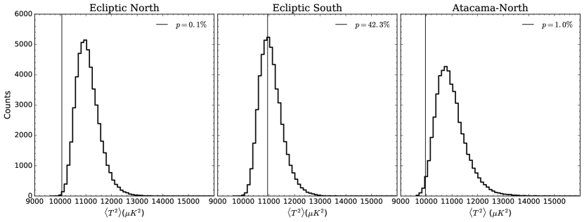
Fig. 1 shows the temperature variance for Ecliptic-North (left), Ecliptic-South (middle), and SMICA-conditioned (right) for unconditioned-CDM. Also plotted as vertical lines are the appropriate values calculated from the Planck SMICA map. While the Ecliptic-South variance has a -value of approximately per cent, meaning that per cent of the theory realizations had a variance equal to or smaller than the one seen in the SMICA map, the Ecliptic-North value corresponds to per cent. This result is in agreement with Akrami et al. (2014) and other hemispherical anomaly studies as summarized in Planck Collaboration et al. (2015b). When the coverage is limited to Atacama-North, the previous full-north per cent measurement becomes a per cent measurement.
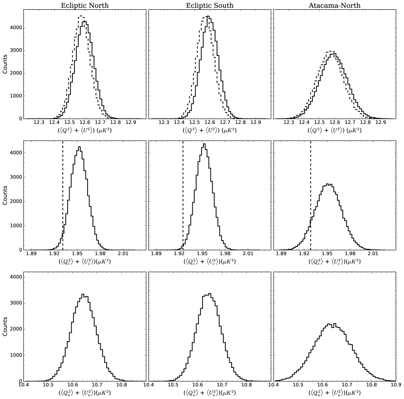
In Fig. 2 the polarization results for are displayed. As in Fig. 1, the left column shows Ecliptic-North, the middle one Ecliptic-South, and the right one SMICA-conditioned. The rows represent the full polarization variance (top), only the portion of polarization correlated with the temperature (middle), and the uncorrelated portion of the polarization (bottom). In each panel, the solid curve represents the results from unconditioned-CDM while the dashed curve represents those from SMICA-conditioned. (There is no SMICA-conditioned result for the uncorrelated portion of the polarization.) As can be seen in the figure, the local lack of power in the temperature map does not directly translate to a localized lack of power in . Instead, its effect is only a slight overall decrease in the variance of the polarization in the SMICA-conditioned set.
The SMICA-conditioned correlated piece (see the middle row of Fig. 2), does indeed show a suppression of the variance, though less so (in terms of p-value) than the temperature. Perhaps surprisingly, this is approximately equally true in the northern and southern hemispheres. This can be attributed to the -weighting applied to when generating the correlated piece of (see Copi et al., 2013, Appendix A). However, the contribution of the correlated piece of SMICA-conditioned is small compared to the uncorrelated piece (third row of Fig. 2).
The results for SMICA-conditioned make it clear that under the fluke hypothesis the polarization is not expected to exhibit the low northern hemisphere variance that is seen in the temperature data. Similarly it would predict no north-south hemispherical asymmetry in the variance. Thus, any detection in next generation polarization maps would be considered as evidence against the fluke hypothesis. Furthermore, if the Ecliptic-North polarization variance data were to suffer a fractional change similar to the one seen in the temperature, of around per cent when compared to Ecliptic-South, the resulting variance of approximately would fall well below the predicted distribution, even with only partial northern sky coverage. (Also see Fig. 3 .)
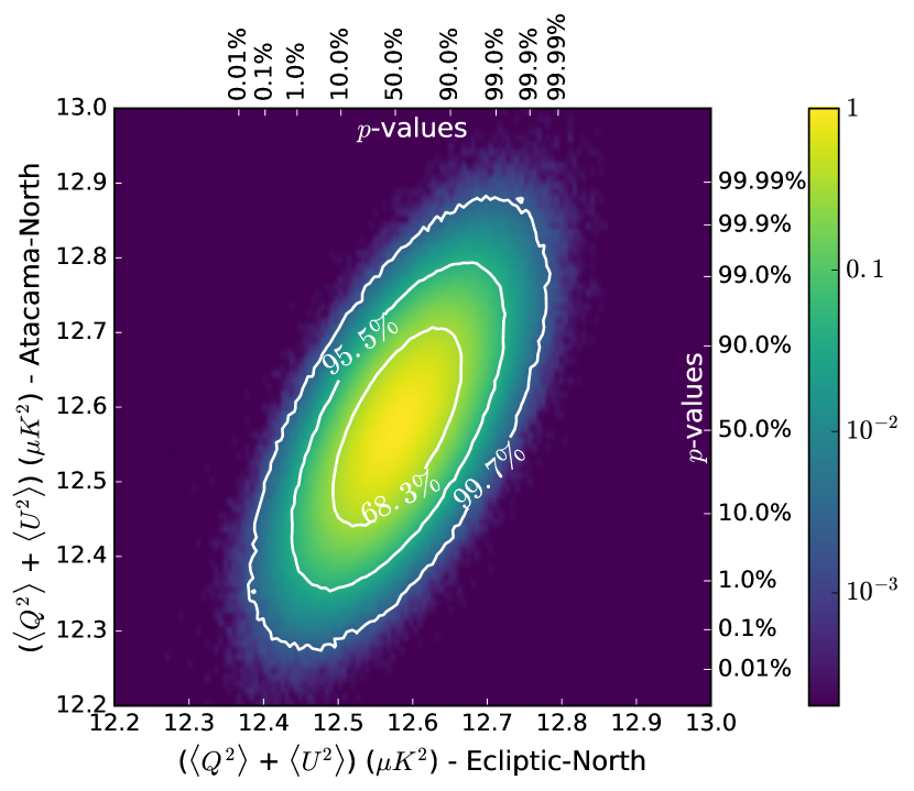
The results for the portion of the north Ecliptic sky seen from the Chilean site (Atacama-North) are displayed in the third column of Fig. 2. We see that, as expected, for a given measured variance that is smaller than the mean value, the -value in Atacama-North will be larger than the -value in the Ecliptic-North as the distributions have the same mean and the former is wider. For any assumed measured variance we could thus work out how much stronger our ability would be to detect anomalous behavior given observations over the whole Ecliptic-North rather than just Atacama-North. However, we only see this if we make the strong assumption that the observed variance in Ecliptic-North is the same as the observed variance in the Atacama-North. We would like to relax this assumption. If we had an actual model that explains the temperature variance anomaly, we could use that model to construct the conditional probability distribution that relates Atacama-North variance to Ecliptic-North variance, and thus construct a joint distribution of -values from which one can infer the probability distribution on Ecliptic-North given a -value in Atacama-North or the -distribution on Atacama-North given a value in Ecliptic-North. These conditionals would then quantify the benefits of measuring the whole Ecliptic-North vs. measuring just Atacama-North. Of course we do not have such a model. We therefore once again use the only model we do have to obtain some guidance: CDM. Specifically, we assume that the fluctuations about some mean variance are the same in our hypothetical anomaly model as in CDM. With that assumption, we can calculate the desired joint probability distribution shown in Fig. 3. The data are displayed as a logarithmic density plot normalized to unity at its peak. Three confidences curves, with probability corresponding to the fraction of points within the curve defined by a constant height, are overlaid. We use an extension of the SMICA-conditioned set with realizations. For each axis, a range of -values is placed on the opposing side of the frame. From this one can deduce how a measurement in Atacama-North with a certain -value translates into the expected range of measurements the theory predicts for the Ecliptic-North coverage scenario or vice versa. For if we expect a -value of per cent on Ecliptic-North, this would lead to a measured p-value on Atacama-North up to a few per cent.
We highlight that we have also studied the impact of sky coverage on the temperature variance utilizing the main method described in Akrami et al. (2014) where a dipole was fit to a local variance map, and the statistics of the dipole amplitude were studied. When comparing methods, simply calculating the variance of the pixels in a hemisphere is particularly good when dealing with small sky coverage. For the specific case of the Atacama-North pixels, we constructed the local temperature variance map on radius disks. From this we found per cent, a substantial decrease in significance. Further, the hemispherical variance method has the added advantage of not depending on an arbitrary choice of disk size.
4 Conclusions
Using the Planck Release-2 SMICA temperature map and the best-fitting Planck (TT + lowP + lensing) parameters (Planck Collaboration et al., 2015d), we have predicted the probability distribution for the variance of the -mode polarization for the full northern Ecliptic sky (Ecliptic-North) and the portion of it that could be observed from a ground based telescope at the high Chilean Atacama plateau (Atacama-North). The latter sky coverage scenario was motivated by the next generation ground-based CMB experiment, CMB-S4, which will most likely include a telescope at the aforementioned site.
From our set of -mode realizations constrained by the observed temperature fluctuations, we have found that within CDM the anomalously low Ecliptic-North variance observed in the temperature results in only a slight overall decrease in the mean of the polarization variance in both the northern and southern, when compared with a set of unconstrained realizations. This decrease is small compared to the widths of the distributions. Neither is any significant asymmetry predicted between the Ecliptic hemispheres. Therefore a future measurement of polarization variance over both northern and southern Ecliptic skies should provide a good test of the fluke hypothesis.
To address the issue of a possible limited northern Ecliptic sky coverage, we compared how a measurement on the full north relates to the piece observed from the Chilean site. The temperature data show a suppression of around per cent in the northern Ecliptic variance when compared to the southern Ecliptic value, or the theoretical mean. Lacking a physical model for this suppression, we cannot predict what the expected signal of such a model would be. However, given that the polarization distributions are much narrower than those for the temperature, a mechanism resulting in a similar fractional suppression of percent, would fall well below the predicted curve (-value per cent) for either Atacama-North or the full North-Ecliptic sky, and would be easily detectable even for just Atacama-North.
For a less extreme suppression of the polarization variance, the advantages of larger northern sky coverage are clearer. In the case of CMB temperature the observed full northern sky -value of per cent becomes a less extreme -value of per cent on the partial northern sky. For polarization, we can predict the probability distribution functions in LCDM given the observed temperature map. As expected full-Northern variance and Atacama-Northern variance are correlated: their probability distributions have the same mean, and low full-Northern variance predicts low Atacama-Northern variance, and vice versa. However, also as expected, reduced sky coverage reduces the significance (increases the p-value) of a measurement of suppressed variance, and we have quantified this. For example, a p-value of percent on the North-Ecliptic sky corresponds to a range of p-values on Atacama-North that can easily reach up to a few percent. This suggests that a larger northern sky coverage would increase the utility of CMB-S4 for probing CMB anomalies, and the hypothesis that they are merely a statistical fluke.
Acknowledgements
GDS and MO’D are partially supported by Department of Energy grant DE-SC0009946 to the particle astrophysics theory group at CWRU. MO’D is partially supported by the CAPES Foundation of the Ministry of Education of Brazil. Some of the results in this paper have been derived using the healpix (Górski et al., 2005) package. This work made use of the High Performance Computing Resource in the Core Facility for Advanced Research Computing at Case Western Reserve University.
References
- Aiola et al. (2015) Aiola S., Wang B., Kosowsky A., Kahniashvili T., Firouzjahi H., 2015, Phys. Rev. D, 92, 063008
- Akrami et al. (2014) Akrami Y., Fantaye Y., Shafieloo A., Eriksen H. K., Hansen F. K., Banday A. J., Górski K. M., 2014, ApJ, 784, L42
- Bennett et al. (2003) Bennett C. L., et al., 2003, ApJ, 583, 1
- Bennett et al. (2011) Bennett C. L., et al., 2011, ApJS, 192, 17
- Copi et al. (2010) Copi C. J., Huterer D., Schwarz D. J., Starkman G. D., 2010, Advances in Astronomy, 2010, 847541
- Copi et al. (2013) Copi C. J., Huterer D., Schwarz D. J., Starkman G. D., 2013, MNRAS, 434, 3590
- Eriksen et al. (2004) Eriksen H. K., Hansen F. K., Banday A. J., Gorski K. M., Lilje P. B., 2004, Astrophys. J., 605, 14
- Górski et al. (2005) Górski K. M., Hivon E., Banday A. J., Wandelt B. D., Hansen F. K., Reinecke M., Bartelmann M., 2005, ApJ, 622, 759
- Namjoo et al. (2015) Namjoo M. H., Abolhasani A. A., Assadullahi H., Baghram S., Firouzjahi H., Wands D., 2015, J. Cosmology Astropart. Phys., 5, 015
- Planck Collaboration et al. (2015a) Planck Collaboration et al., 2015a, preprint, (arXiv:1502.05956)
- Planck Collaboration et al. (2015c) Planck Collaboration et al., 2015c, preprint, (arXiv:1509.06348)
- Planck Collaboration et al. (2015d) Planck Collaboration et al., 2015d, preprint, (arXiv:1502.01589)
- Planck Collaboration et al. (2015b) Planck Collaboration et al., 2015b, preprint, (arXiv:1506.07135)
- Quartin & Notari (2015) Quartin M., Notari A., 2015, J. Cosmology Astropart. Phys., 1, 008
- Schwarz et al. (2015) Schwarz D. J., Copi C. J., Huterer D., Starkman G. D., 2015, preprint, (arXiv:1510.07929)