An EM algorithm for absolutely continuous Marshall-Olkin bivariate Pareto distribution with location and scale

Abstract

In this paper, we have considered a Block-Basu type bivariate Pareto distribution. Here in the standard manner, first Marshall-Olkin type singular bivariate distribution has been constructed, and then by taking away the singular component similar to the Block and Basu model, an absolute continuous BB-BVPA model has been constructed. Further, the location and scale parameters also have been introduced. Therefore, the model has seven parameters. Different properties of this absolutely continuous distribution are derived. Since the maximum likelihood estimators of the parameters cannot be expressed in a closed form, we propose to use an EM algorithm to compute the estimators of the model parameters. Some simulation experiments have been performed for illustrative purposes. The model is fitted to rainfall data in the context of landslide risk estimation.

Biplab Paul1, Arabin Kumar Dey2

1Department of Statistics, University of Haifa, Israel

2 Department of Mathematics, IIT Guwahati, India

00footnotetext: Correspondence author’s Email address: paul.biplab497@gmail.com (Biplab Paul)

Keywords: Absolute Continuous Distribution; Bivariate Pareto distribution; Confidence interval; Expectation-maximization algorithm; Landslides; Marshall-Olkin bivariate Pareto distribution.

1 Introduction

Statistical inference for extreme values has received extensive attention over the past couple of decades. They are extensively discussed by Coles et al. [7], Embrechts et al. [11], Kotz and Nadarajah [16], Reiss and Thomas [32], and so on. Pareto distribution plays an important role in extreme value (EV) theory. It is noted that there is an intimate relation between the Pareto type II𝐼𝐼II distribution and the Pickands generalized Pareto model [see, e.g., 1]. Different variants of the classical Pareto distributions are typically used to analyze income and wealth data. Bivariate Pareto has a wide application in many applied areas, including finance, failure times, income and wealth modeling, insurance, environmental sciences, internet network, modeling of birth rates and infant mortality rates, reliability, etc. In a financial setting, multivariate Pareto distribution can be used to model the dependent risks associated with lines of business [see, e.g., 34]. This distribution might be used to estimate system reliability in stress-strength setting [see, e.g., 13]. Multivariate Pareto distribution is also useful to measure the impact of extreme events, which often depend on not just a single component but the combined behavior of several components of interest.

Even though different types of univariate Pareto distributions [see, e.g., 2, 3] have been analyzed extensively, there is a lack of methods for analyzing multivariate Pareto distributions. In 1962, Mardia [24] first systematically studied multivariate Pareto distribution where marginals are Pareto type I𝐼I distribution with common shape parameter. Arnold [1] proposed multivariate Pareto distribution type II𝐼𝐼II using same procedure as in Mardia [24]. The Bivariate Lomax distribution proposed by Lindley and Singpurwalla [23] is another popular bivariate Pareto distribution, which also has Lomax marginals. A detailed description of multivariate Pareto distribution can be found in [1]. In this context, a book by Kotz et al. [17] can be a good reference. However, inference methods for various forms of multivariate Pareto distributions have been somewhat restricted. The main reason for this limitation is a lack of appropriate models which predict multivariate Paretian behavior. Recently Asimit et al. [4] proposed Marshall-Olkin bivariate Pareto (MOBVPA) distribution using the same procedure as in [26] and used the Expectation-maximization (EM) algorithm to estimate the unknown parameters. Dey and Paul [8] also described other innovative variations of the EM algorithm to estimate the unknown parameters of the MOBVPA model. MOBVPA distribution works quite effectively to analyze data when some of the two components of standardized dataset (location-scale transformation) take equal values because it is a singular distribution. In real-life datasets, we do not know the exact value of location and scale parameters, so it is quite impossible to know whether the standardized dataset has equal components. Therefore, this MOBVPA model with location and scale leads to misleading results when the standardized dataset does not have equal components.

In 1974, Block and Basu [6] proposed the bivariate exponential distribution (BBBE) from the Marshall-Olkin bivariate exponential (MOBE) distribution by removing the singular part and retaining only the absolutely continuous part. This BBBE distribution is one of the most popular and widely used absolutely continuous bivariate distributions because, unlike MOBE, it enjoys all the properties of an absolutely continuous distribution. Interestingly, marginals are not the exponential distributions.

Along the same line as BBBE distribution [see, e.g., 6], Block-Basu bivariate Pareto (hereafter called BB-BVPA) distribution has been defined. This distribution has been obtained from the MOBVPA distribution by removing the singular part, which makes the BB-BVPA distribution an absolutely continuous bivariate distribution. Similar to the MOBVPA model, BB-BVPA also has seven parameters. Although extensive works [see, e.g., 18, 19, 20, 21, 22, 27] have been done on the absolutely continuous version of MOBE and MOBW models, not that much of attention has been paid on BB-BVPA model. The reason might be, computationally it may not be very tractable, especially in the presence of both location and scale parameters. In fact, computing the maximum likelihood estimators (MLEs) of the unknown parameters of the BB-BVPA model in the location and scale parameters is not a trivial issue. Only recently, Paul et al. [30] proposed a Bayesian inference procedure for BB-BVPA distribution without location and scale parameters. We introduce location and scale parameters to the BB-BVPA model; hence it brings more flexibility. Unlike the bivariate Pareto distribution by Arnold [1], Lindley and Singpurwalla [23] and Mardia [24], the marginals of BB-BVPA do not have a common shape parameter due to the presence of multiple shape parameters in the BB-BVPA model, which gives more flexibility. Although the marginals of BB-BVPA are not Pareto type II𝐼𝐼II in general, the shape of the PDF of marginals is very similar to the PDF of a Pareto type II𝐼𝐼II distribution. Interestingly, for non-negative location parameters, the distribution of these marginals are weighted distributions corresponding to Pareto type II𝐼𝐼II distribution, and, hence, the properties of weighted distribution [see, e.g., 28] are also available here. Moreover, without any restriction on model parameters, we have shown that the BB-BVPA model without location and scale parameters has total positivity of order 222 (TP2𝑇subscript𝑃2TP_{2}). This distribution also has some properties which have proved useful for reliability applications. To the best of our knowledge, the formulation and estimation methodologies of the BB-BVPA distribution with location and scale parameters are yet to be developed.

In this article, different properties and different computational issues associated in computing the unknown parameters of the BB-BVPA distribution are discussed. First, we consider the computation of MLEs of the seven unknown parameters of the BB-BVPA model. As expected, the MLEs cannot be obtained in explicit form. To compute the MLEs directly, one needs to solve a multi-dimensional optimization problem. It is observed that the EM algorithm can be used quite effectively to compute MLEs of parameters of BB-BVPA. At each EM step (iteration), one needs to solve only a one-dimensional optimization problem, and we have proposed a simple procedure to solve this problem. It should be mentioned that the usual gradient descent does not work as the bivariate likelihood is a discontinuous function for the location and scale parameters. We suggest a novel way to handle all related computational problems which work most efficiently. The first contribution of this article is to implement the EM algorithm for the three-parameter BB-BVPA model without location and scale parameters, where a crucial modification of the EM algorithm is suggested to make the algorithm work for any range of parameters. The other contribution is an exploration of an efficient EM algorithm that will work in the case of the seven-parameter setup. The suggested structure combines several ideas, including previously suggested modification of the three-parameter setup. The distribution can be used quite effectively for the data transformed via the peak over threshold method, especially when the transformed dataset does not have equal component observations. The dependence structure of this absolute continuous version can also be described by the well-known Marshall-Olkin copula [see, e.g., 25, 29]. It should be noted that the methodology proposed here works quite well for moderately large samples. We also propose to use a naive construction of confidence interval for the parameters.

We illustrate the usefulness of this BB-BVPA model by fitting it to extreme precipitation data and by showing how the results could be used to estimate risks for landslides. Extreme precipitation has a number of potentially hazardous consequences, such as flooding, plugged drainage systems, wasted crops and landslides. This analysis also helps to plot insurance policies to compensate for the losses or damage caused by floods, landslides, etc.

The organization of the paper is as follows. A brief description of the formulation and different properties of BB-BVPA distribution are given in Section 2. Section 3 is kept for different extensions of the EM algorithm of BB-BVPA distribution. We discuss the construction of confidence interval in Section 4. Some simulated datasets are analyzed in Section 5 for illustrative purposes. Section 6, we fit our BB-BVPA model to rainfall data in the context of landslide risk estimation. Finally, Section 7 contains a brief summary of the work and some concluding remarks.

2 Formulation of Block-Basu bivariate Pareto distribution

If a random variable X𝑋X has a univariate Pareto type II𝐼𝐼II distribution with the location, scale and shape parameters as μ𝜇\mu\in\mathbb{R}, σ>0𝜎0\sigma>0 and α>0𝛼0\alpha>0, respectively, then for x>μ𝑥𝜇x>\mu, the probability density function (PDF) and survival function (SE) are defined as follows;

fPA(x;μ,σ,α)=ασ(1+xμσ)α1,SPA(x;μ,σ,α)=(1+xμσ)α,formulae-sequencesubscript𝑓𝑃𝐴𝑥𝜇𝜎𝛼𝛼𝜎superscript1𝑥𝜇𝜎𝛼1subscript𝑆𝑃𝐴𝑥𝜇𝜎𝛼superscript1𝑥𝜇𝜎𝛼f_{PA}(x;\mu,\sigma,\alpha)=\dfrac{\alpha}{\sigma}\Big{(}1+\dfrac{x-\mu}{\sigma}\Big{)}^{-\alpha-1},~{}~{}S_{PA}(x;\mu,\sigma,\alpha)=\Big{(}1+\frac{x-\mu}{\sigma}\Big{)}^{-\alpha}, (1)

respectively. From now on a Pareto type II𝐼𝐼II distribution with the PDF (1) will be denoted by PA(II)(μ,σ,α)𝑃𝐴𝐼𝐼𝜇𝜎𝛼PA(II)(\mu,\sigma,\alpha). Let us consider U0subscript𝑈0U_{0} follows ()PA(II)(0,1,α0)similar-to𝑃𝐴𝐼𝐼01subscript𝛼0(\sim)PA(II)(0,1,\alpha_{0}), U1PA(II)(μ1,σ1,α1)similar-tosubscript𝑈1𝑃𝐴𝐼𝐼subscript𝜇1subscript𝜎1subscript𝛼1U_{1}\sim PA(II)(\mu_{1},\sigma_{1},\alpha_{1}) and U2PA(II)(μ2,σ2,α2)similar-tosubscript𝑈2𝑃𝐴𝐼𝐼subscript𝜇2subscript𝜎2subscript𝛼2U_{2}\sim PA(II)(\mu_{2},\sigma_{2},\alpha_{2}) and also they are mutually independent. Define X1=min{σ1U0+μ1,U1}subscript𝑋1subscript𝜎1subscript𝑈0subscript𝜇1subscript𝑈1X_{1}=\min\{\sigma_{1}U_{0}+\mu_{1},U_{1}\} and X2=min{σ2U0+μ2,U2}subscript𝑋2subscript𝜎2subscript𝑈0subscript𝜇2subscript𝑈2X_{2}=\min\{\sigma_{2}U_{0}+\mu_{2},U_{2}\}, then the bivariate random variable (X1,X2)subscript𝑋1subscript𝑋2(X_{1},X_{2}) has MOBVPA distribution with parameters (μ1,μ2,σ1,σ2,α0,α1,α2)subscript𝜇1subscript𝜇2subscript𝜎1subscript𝜎2subscript𝛼0subscript𝛼1subscript𝛼2(\mu_{1},\mu_{2},\sigma_{1},\sigma_{2},\alpha_{0},\alpha_{1},\alpha_{2}) and it will be denoted from now on as MOBVPA(μ1,μ2,σ1,MOBVPA(\mu_{1},\mu_{2},\sigma_{1}, σ2,α0,α1,α2)\sigma_{2},\alpha_{0},\alpha_{1},\alpha_{2}). The joint PDF of (X1,X2)subscript𝑋1subscript𝑋2(X_{1},X_{2}) is

f(x1,x2)={f1(x1,x2),if x1μ1σ1 <x2μ2σ2f2(x1,x2),if x1μ1σ1 >x2μ2σ2f0(x),if x1μ1σ1 = x2μ2σ2=x,𝑓subscript𝑥1subscript𝑥2casessubscript𝑓1subscript𝑥1subscript𝑥2if x1μ1σ1 <x2μ2σ2otherwisesubscript𝑓2subscript𝑥1subscript𝑥2if x1μ1σ1 >x2μ2σ2otherwisesubscript𝑓0𝑥if x1μ1σ1 = x2μ2σ2𝑥otherwisef(x_{1},x_{2})=\begin{cases}f_{1}(x_{1},x_{2}),~{}\text{if $\frac{x_{1}-\mu_{1}}{\sigma_{1}}$ \textless$\frac{x_{2}-\mu_{2}}{\sigma_{2}}$}\\ f_{2}(x_{1},x_{2}),~{}\text{if $\frac{x_{1}-\mu_{1}}{\sigma_{1}}$ \textgreater$\frac{x_{2}-\mu_{2}}{\sigma_{2}}$}\\ f_{0}(x),~{}\text{if $\frac{x_{1}-\mu_{1}}{\sigma_{1}}$ = $\frac{x_{2}-\mu_{2}}{\sigma_{2}}$}=x,\end{cases} (2)

where

f1(x1,x2)=α1(α0+α2)σ1σ2(1+x2μ2σ2)α0α21(1+x1μ1σ1)α11f2(x1,x2)=α2(α0+α1)σ1σ2(1+x2μ2σ2)α21(1+x1μ1σ1)α0α11f0(x)=α0(1+x)α0α1α21.subscript𝑓1subscript𝑥1subscript𝑥2subscript𝛼1subscript𝛼0subscript𝛼2subscript𝜎1subscript𝜎2superscript1subscript𝑥2subscript𝜇2subscript𝜎2subscript𝛼0subscript𝛼21superscript1subscript𝑥1subscript𝜇1subscript𝜎1subscript𝛼11subscript𝑓2subscript𝑥1subscript𝑥2subscript𝛼2subscript𝛼0subscript𝛼1subscript𝜎1subscript𝜎2superscript1subscript𝑥2subscript𝜇2subscript𝜎2subscript𝛼21superscript1subscript𝑥1subscript𝜇1subscript𝜎1subscript𝛼0subscript𝛼11subscript𝑓0𝑥subscript𝛼0superscript1𝑥subscript𝛼0subscript𝛼1subscript𝛼21\begin{split}f_{1}(x_{1},x_{2})&=\frac{\alpha_{1}(\alpha_{0}+\alpha_{2})}{\sigma_{1}\sigma_{2}}\Big{(}1+\frac{x_{2}-\mu_{2}}{\sigma_{2}}\Big{)}^{-\alpha_{0}-\alpha_{2}-1}\Big{(}1+\frac{x_{1}-\mu_{1}}{\sigma_{1}}\Big{)}^{-\alpha_{1}-1}\\ f_{2}(x_{1},x_{2})&=\frac{\alpha_{2}(\alpha_{0}+\alpha_{1})}{\sigma_{1}\sigma_{2}}\Big{(}1+\frac{x_{2}-\mu_{2}}{\sigma_{2}}\Big{)}^{-\alpha_{2}-1}\Big{(}1+\frac{x_{1}-\mu_{1}}{\sigma_{1}}\Big{)}^{-\alpha_{0}-\alpha_{1}-1}\\ f_{0}(x)&=\alpha_{0}(1+x)^{-\alpha_{0}-\alpha_{1}-\alpha_{2}-1}.\end{split}

When μ1=μ2=0subscript𝜇1subscript𝜇20\mu_{1}=\mu_{2}=0 and σ1=σ2=1subscript𝜎1subscript𝜎21\sigma_{1}=\sigma_{2}=1, we call it three-parameter MOBVPA distribution and will be denoted by MOBVPA(α0,α1,α2)𝑀𝑂𝐵𝑉𝑃𝐴subscript𝛼0subscript𝛼1subscript𝛼2MOBVPA(\alpha_{0},\alpha_{1},\alpha_{2}). Note that Block-Basu bivariate Pareto distribution can be obtained from MOBVPA distribution by removing the singular part and keeping only the continuous part. The joint PDF of BB-BVPA distribution is

fBB(y1,y2)subscript𝑓𝐵𝐵subscript𝑦1subscript𝑦2\displaystyle f_{BB}(y_{1},y_{2}) ={cf1(y1,y2)if y1μ1σ1<y2μ2σ2cf2(y1,y2)if y1μ1σ1>y2μ2σ2,absentcases𝑐subscript𝑓1subscript𝑦1subscript𝑦2if y1μ1σ1<y2μ2σ2otherwise𝑐subscript𝑓2subscript𝑦1subscript𝑦2if y1μ1σ1>y2μ2σ2otherwise\displaystyle=\begin{cases}cf_{1}(y_{1},y_{2})~{}~{}\text{if $\frac{y_{1}-\mu_{1}}{\sigma_{1}}<\frac{y_{2}-\mu_{2}}{\sigma_{2}}$}\\ cf_{2}(y_{1},y_{2})~{}~{}\text{if $\frac{y_{1}-\mu_{1}}{\sigma_{1}}>\frac{y_{2}-\mu_{2}}{\sigma_{2}}$},\end{cases} (3)

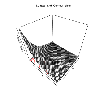
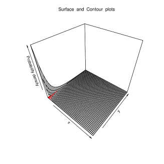
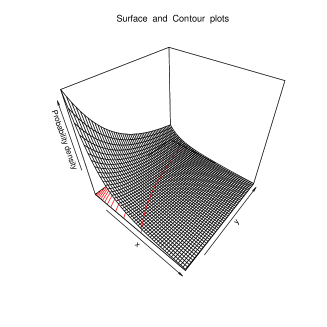
where c is a normalizing constant and c=α0+α1+α2α1+α2𝑐subscript𝛼0subscript𝛼1subscript𝛼2subscript𝛼1subscript𝛼2c=\frac{\alpha_{0}+\alpha_{1}+\alpha_{2}}{\alpha_{1}+\alpha_{2}}. Therefore, the joint PDF of bivariate random variable (Y1,Y2)subscript𝑌1subscript𝑌2(Y_{1},Y_{2}) can be written as (3) and it will be denoted as BBBVPA(μ1,μ2,σ1,σ2,α0,α1,α2)𝐵𝐵𝐵𝑉𝑃𝐴subscript𝜇1subscript𝜇2subscript𝜎1subscript𝜎2subscript𝛼0subscript𝛼1subscript𝛼2BBBVPA(\mu_{1},\mu_{2},\sigma_{1},\sigma_{2},\alpha_{0},\alpha_{1},\alpha_{2}). The joint PDF of (Y1,Y2)subscript𝑌1subscript𝑌2(Y_{1},Y_{2}) is unimodal. Surface and contour plots of fBB(y1,y2)subscript𝑓𝐵𝐵subscript𝑦1subscript𝑦2f_{BB}(y_{1},y_{2}) for different values of parameters are shown in Figure 2. When μ1=μ2=0subscript𝜇1subscript𝜇20\mu_{1}=\mu_{2}=0 and σ1=σ2=1subscript𝜎1subscript𝜎21\sigma_{1}=\sigma_{2}=1, we call it three-parameter BB-BVPA distribution and denote this distribution as BBBVPA(α0,α1,α2)𝐵𝐵𝐵𝑉𝑃𝐴subscript𝛼0subscript𝛼1subscript𝛼2BBBVPA(\alpha_{0},\alpha_{1},\alpha_{2}).

2.1 Properties

Different properties of this BB-BVPA distribution are studied here. First, we provide the marginal and conditional distributions of the BB-BVPA distribution.

Theorem 1.

If (Y1,Y2)subscript𝑌1subscript𝑌2(Y_{1},Y_{2}) similar-to\sim BBBVPA(μ1,μ2,σ1,σ2,α0,α1,α2)𝐵𝐵𝐵𝑉𝑃𝐴subscript𝜇1subscript𝜇2subscript𝜎1subscript𝜎2subscript𝛼0subscript𝛼1subscript𝛼2BBBVPA(\mu_{1},\mu_{2},\sigma_{1},\sigma_{2},\alpha_{0},\alpha_{1},\alpha_{2}), then the marginal PDFs of Y1subscript𝑌1Y_{1} and Y2subscript𝑌2Y_{2} are as follows

fY1(y1)=cfPA(y1;μ1,σ1,α0+α1)α0(α1+α2)fPA(y1;μ1,σ1,α0+α1+α2)subscript𝑓subscript𝑌1subscript𝑦1𝑐subscript𝑓𝑃𝐴subscript𝑦1subscript𝜇1subscript𝜎1subscript𝛼0subscript𝛼1subscript𝛼0subscript𝛼1subscript𝛼2subscript𝑓𝑃𝐴subscript𝑦1subscript𝜇1subscript𝜎1subscript𝛼0subscript𝛼1subscript𝛼2\displaystyle f_{Y_{1}}(y_{1})=cf_{PA}(y_{1};\mu_{1},\sigma_{1},\alpha_{0}+\alpha_{1})-\frac{\alpha_{0}}{(\alpha_{1}+\alpha_{2})}f_{PA}(y_{1};\mu_{1},\sigma_{1},\alpha_{0}+\alpha_{1}+\alpha_{2})

and

fY2(y2)=cfPA(y2;μ2,σ2,α0+α2)α0(α1+α2)fPA(y2;μ2,σ2,α0+α1+α2),subscript𝑓subscript𝑌2subscript𝑦2𝑐subscript𝑓𝑃𝐴subscript𝑦2subscript𝜇2subscript𝜎2subscript𝛼0subscript𝛼2subscript𝛼0subscript𝛼1subscript𝛼2subscript𝑓𝑃𝐴subscript𝑦2subscript𝜇2subscript𝜎2subscript𝛼0subscript𝛼1subscript𝛼2\displaystyle f_{Y_{2}}(y_{2})=cf_{PA}(y_{2};\mu_{2},\sigma_{2},\alpha_{0}+\alpha_{2})-\frac{\alpha_{0}}{(\alpha_{1}+\alpha_{2})}f_{PA}(y_{2};\mu_{2},\sigma_{2},\alpha_{0}+\alpha_{1}+\alpha_{2}),

respectively, where c=α0+α1+α2α1+α2𝑐subscript𝛼0subscript𝛼1subscript𝛼2subscript𝛼1subscript𝛼2c=\frac{\alpha_{0}+\alpha_{1}+\alpha_{2}}{\alpha_{1}+\alpha_{2}}.

Proof..

They can be obtained by the definition of marginal distribution from the joint distribution. ∎

Now we mainly discuss some basic properties of marginal Y1subscript𝑌1Y_{1}. The properties of Y2subscript𝑌2Y_{2} are exactly the same. The marginal survival functions of Y1subscript𝑌1Y_{1} is

SY1(y1)=cSPA(y1;μ1,σ1,α0+α1)α0α1+α2SPA(y1;μ1,σ1,α0+α1+α2).subscript𝑆subscript𝑌1subscript𝑦1𝑐subscript𝑆𝑃𝐴subscript𝑦1subscript𝜇1subscript𝜎1subscript𝛼0subscript𝛼1subscript𝛼0subscript𝛼1subscript𝛼2subscript𝑆𝑃𝐴subscript𝑦1subscript𝜇1subscript𝜎1subscript𝛼0subscript𝛼1subscript𝛼2\displaystyle S_{Y_{1}}(y_{1})=cS_{PA}(y_{1};\mu_{1},\sigma_{1},\alpha_{0}+\alpha_{1})-\frac{\alpha_{0}}{\alpha_{1}+\alpha_{2}}S_{PA}(y_{1};\mu_{1},\sigma_{1},\alpha_{0}+\alpha_{1}+\alpha_{2}).

The hazard function (HF) of Y1subscript𝑌1Y_{1} is the following:

hY1(y1)=(α0+α1+α2)(1+y1μ1σ1)1σ1[1α2(α0+α1+α2)α0(1+y1μ1σ1)α2].subscriptsubscript𝑌1subscript𝑦1subscript𝛼0subscript𝛼1subscript𝛼2superscript1subscript𝑦1subscript𝜇1subscript𝜎11subscript𝜎1delimited-[]1subscript𝛼2subscript𝛼0subscript𝛼1subscript𝛼2subscript𝛼0superscript1subscript𝑦1subscript𝜇1subscript𝜎1subscript𝛼2\displaystyle h_{Y_{1}}(y_{1})=\frac{(\alpha_{0}+\alpha_{1}+\alpha_{2})(1+\frac{y_{1}-\mu_{1}}{\sigma_{1}})^{-1}}{\sigma_{1}}\Bigg{[}1-\frac{\alpha_{2}}{(\alpha_{0}+\alpha_{1}+\alpha_{2})-\alpha_{0}(1+\frac{y_{1}-\mu_{1}}{\sigma_{1}})^{-\alpha_{2}}}\Bigg{]}.

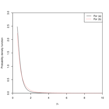
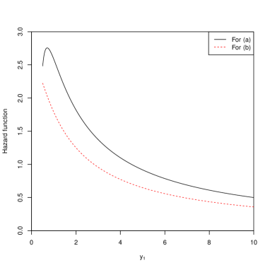
The PDFs and HFs of Y1subscript𝑌1Y_{1} for different values of model parameters are shown in Figure 1. Although the hazard function of Pareto type II𝐼𝐼II is decreasing, interestingly, for some values of model parameters, this function first increases and then decreases. For μ10subscript𝜇10\mu_{1}\geq 0, the distribution of marginal Y1subscript𝑌1Y_{1} can be written as a weighted distribution corresponding to PA(II)(μ1,σ1,α0+α1)𝑃𝐴𝐼𝐼subscript𝜇1subscript𝜎1subscript𝛼0subscript𝛼1PA(II)(\mu_{1},\sigma_{1},\alpha_{0}+\alpha_{1}) with weight function proportional to

w1(y1)=1α0α0+α1(1+y1μ1σ1)α2,subscript𝑤1subscript𝑦11subscript𝛼0subscript𝛼0subscript𝛼1superscript1subscript𝑦1subscript𝜇1subscript𝜎1subscript𝛼2w_{1}(y_{1})=1-\frac{\alpha_{0}}{\alpha_{0}+\alpha_{1}}\bigg{(}1+\frac{y_{1}-\mu_{1}}{\sigma_{1}}\bigg{)}^{-\alpha_{2}},

which is non-negative function with finite non-zero expectation. Hence, the properties available for the weighted distributions can also be applied here.
Refer to caption
(a) Probability density functions.
Refer to caption
(b) Hazard functions.
Figure 1: Probability and hazard functions for (a): μ1=0.5,σ1=1.5,α0=2.75,α1=2.75,α2=5.0formulae-sequencesubscript𝜇10.5formulae-sequencesubscript𝜎11.5formulae-sequencesubscript𝛼02.75formulae-sequencesubscript𝛼12.75subscript𝛼25.0\mu_{1}=0.5,\sigma_{1}=1.5,\alpha_{0}=2.75,\alpha_{1}=2.75,\alpha_{2}=5.0 and (b): μ1=0.5,σ1=1.5,α0=2.0,α1=2.0,α2=1.0formulae-sequencesubscript𝜇10.5formulae-sequencesubscript𝜎11.5formulae-sequencesubscript𝛼02.0formulae-sequencesubscript𝛼12.0subscript𝛼21.0\mu_{1}=0.5,\sigma_{1}=1.5,\alpha_{0}=2.0,\alpha_{1}=2.0,\alpha_{2}=1.0.
Refer to caption
(a) μ1=0,μ2=0,σ1=1,σ2=0.5,α0=1,α1=0.3,α2=1.4formulae-sequencesubscript𝜇10formulae-sequencesubscript𝜇20formulae-sequencesubscript𝜎11formulae-sequencesubscript𝜎20.5formulae-sequencesubscript𝛼01formulae-sequencesubscript𝛼10.3subscript𝛼21.4\mu_{1}=0,\mu_{2}=0,\sigma_{1}=1,\sigma_{2}=0.5,\alpha_{0}=1,\alpha_{1}=0.3,\alpha_{2}=1.4
Refer to caption
(b) μ1=1,μ2=2,σ1=0.4,σ2=0.5,α0=2,α1=1.2,α2=1.4formulae-sequencesubscript𝜇11formulae-sequencesubscript𝜇22formulae-sequencesubscript𝜎10.4formulae-sequencesubscript𝜎20.5formulae-sequencesubscript𝛼02formulae-sequencesubscript𝛼11.2subscript𝛼21.4\mu_{1}=1,\mu_{2}=2,\sigma_{1}=0.4,\sigma_{2}=0.5,\alpha_{0}=2,\alpha_{1}=1.2,\alpha_{2}=1.4
Refer to caption
(c) μ1=0,μ2=0,σ1=1.4,σ2=0.5,α0=1,α1=1,α2=1.4formulae-sequencesubscript𝜇10formulae-sequencesubscript𝜇20formulae-sequencesubscript𝜎11.4formulae-sequencesubscript𝜎20.5formulae-sequencesubscript𝛼01formulae-sequencesubscript𝛼11subscript𝛼21.4\mu_{1}=0,\mu_{2}=0,\sigma_{1}=1.4,\sigma_{2}=0.5,\alpha_{0}=1,\alpha_{1}=1,\alpha_{2}=1.4
Refer to caption
(d) μ1=0,μ2=0,σ1=1.4,σ2=0.5,α0=2,α1=0.4,α2=0.5formulae-sequencesubscript𝜇10formulae-sequencesubscript𝜇20formulae-sequencesubscript𝜎11.4formulae-sequencesubscript𝜎20.5formulae-sequencesubscript𝛼02formulae-sequencesubscript𝛼10.4subscript𝛼20.5\mu_{1}=0,\mu_{2}=0,\sigma_{1}=1.4,\sigma_{2}=0.5,\alpha_{0}=2,\alpha_{1}=0.4,\alpha_{2}=0.5
Figure 2: Surface and contour plots of PDF of BB-BVPA for different values of parameters.

From Theorem 1, it is clear that the distribution of Y1subscript𝑌1Y_{1} is not Pareto type II𝐼𝐼II distribution in general. Although the PDF of Y1subscript𝑌1Y_{1} is not Pareto type II𝐼𝐼II in general, the shape of the PDF of Y1subscript𝑌1Y_{1} is very similar to the PDF of a Pareto type II𝐼𝐼II distribution. Now we discuss the conditional probability density functions.

Theorem 2.

If (Y1,Y2)subscript𝑌1subscript𝑌2(Y_{1},Y_{2}) similar-to\sim BBBVPA(μ1,μ2,σ1,σ2,α0,α1,α2)𝐵𝐵𝐵𝑉𝑃𝐴subscript𝜇1subscript𝜇2subscript𝜎1subscript𝜎2subscript𝛼0subscript𝛼1subscript𝛼2BBBVPA(\mu_{1},\mu_{2},\sigma_{1},\sigma_{2},\alpha_{0},\alpha_{1},\alpha_{2}), then the conditional PDFs of Y1|Y2=y2conditionalsubscript𝑌1subscript𝑌2subscript𝑦2Y_{1}|Y_{2}=y_{2} and Y2|Y1=y1conditionalsubscript𝑌2subscript𝑌1subscript𝑦1Y_{2}|Y_{1}=y_{1} are as follows

fY1|Y2(y1|y2)={(α0+α2)fPA(y1;μ1,σ1,α1)α2+α0{1(1+y2μ2σ2)α1},if y1μ1σ1 <y2μ2σ2α2fPA(y1;μ1,σ1,α0+α1)(1+y2μ2σ2)α0[α2+α0{1(1+y2μ2σ2)α1}],if y1μ1σ1 >y2μ2σ2subscript𝑓conditionalsubscript𝑌1subscript𝑌2conditionalsubscript𝑦1subscript𝑦2casessubscript𝛼0subscript𝛼2subscript𝑓𝑃𝐴subscript𝑦1subscript𝜇1subscript𝜎1subscript𝛼1subscript𝛼2subscript𝛼01superscript1subscript𝑦2subscript𝜇2subscript𝜎2subscript𝛼1if y1μ1σ1 <y2μ2σ2otherwisesubscript𝛼2subscript𝑓𝑃𝐴subscript𝑦1subscript𝜇1subscript𝜎1subscript𝛼0subscript𝛼1superscript1subscript𝑦2subscript𝜇2subscript𝜎2subscript𝛼0delimited-[]subscript𝛼2subscript𝛼01superscript1subscript𝑦2subscript𝜇2subscript𝜎2subscript𝛼1if y1μ1σ1 >y2μ2σ2otherwise\displaystyle f_{Y_{1}|Y_{2}}(y_{1}|y_{2})=\begin{cases}\frac{(\alpha_{0}+\alpha_{2})f_{PA}(y_{1};\mu_{1},\sigma_{1},\alpha_{1})}{\alpha_{2}+\alpha_{0}\big{\{}1-\left(1+\frac{y_{2}-\mu_{2}}{\sigma_{2}}\right)^{-\alpha_{1}}\big{\}}},~{}\text{if $\frac{y_{1}-\mu_{1}}{\sigma_{1}}$ \textless$\frac{y_{2}-\mu_{2}}{\sigma_{2}}$}\\ \frac{\alpha_{2}f_{PA}(y_{1};\mu_{1},\sigma_{1},\alpha_{0}+\alpha_{1})}{\left(1+\frac{y_{2}-\mu_{2}}{\sigma_{2}}\right)^{-\alpha_{0}}\big{[}\alpha_{2}+\alpha_{0}\big{\{}1-\left(1+\frac{y_{2}-\mu_{2}}{\sigma_{2}}\right)^{-\alpha_{1}}\big{\}}\big{]}},~{}\text{if $\frac{y_{1}-\mu_{1}}{\sigma_{1}}$ \textgreater$\frac{y_{2}-\mu_{2}}{\sigma_{2}}$}\end{cases} (4)

and

fY2|Y1(y2|y1)={α1fPA(y2;μ2,σ2,α0+α2)(1+y1μ1σ1)α0[α1+α0{1(1+y1μ1σ1)α2}],if y1μ1σ1 <y2μ2σ2(α0+α1)fPA(y2;μ2,σ2,α2)α1+α0{1(1+y1μ1σ1)α2},if y1μ1σ1 >y2μ2σ2,subscript𝑓conditionalsubscript𝑌2subscript𝑌1conditionalsubscript𝑦2subscript𝑦1casessubscript𝛼1subscript𝑓𝑃𝐴subscript𝑦2subscript𝜇2subscript𝜎2subscript𝛼0subscript𝛼2superscript1subscript𝑦1subscript𝜇1subscript𝜎1subscript𝛼0delimited-[]subscript𝛼1subscript𝛼01superscript1subscript𝑦1subscript𝜇1subscript𝜎1subscript𝛼2if y1μ1σ1 <y2μ2σ2otherwisesubscript𝛼0subscript𝛼1subscript𝑓𝑃𝐴subscript𝑦2subscript𝜇2subscript𝜎2subscript𝛼2subscript𝛼1subscript𝛼01superscript1subscript𝑦1subscript𝜇1subscript𝜎1subscript𝛼2if y1μ1σ1 >y2μ2σ2otherwise\displaystyle f_{Y_{2}|Y_{1}}(y_{2}|y_{1})=\begin{cases}\frac{\alpha_{1}f_{PA}(y_{2};\mu_{2},\sigma_{2},\alpha_{0}+\alpha_{2})}{\left(1+\frac{y_{1}-\mu_{1}}{\sigma_{1}}\right)^{-\alpha_{0}}\big{[}\alpha_{1}+\alpha_{0}\big{\{}1-\left(1+\frac{y_{1}-\mu_{1}}{\sigma_{1}}\right)^{-\alpha_{2}}\big{\}}\big{]}},~{}\text{if $\frac{y_{1}-\mu_{1}}{\sigma_{1}}$ \textless$\frac{y_{2}-\mu_{2}}{\sigma_{2}}$}\\ \frac{(\alpha_{0}+\alpha_{1})f_{PA}(y_{2};\mu_{2},\sigma_{2},\alpha_{2})}{\alpha_{1}+\alpha_{0}\big{\{}1-\left(1+\frac{y_{1}-\mu_{1}}{\sigma_{1}}\right)^{-\alpha_{2}}\big{\}}},~{}\text{if $\frac{y_{1}-\mu_{1}}{\sigma_{1}}$ \textgreater$\frac{y_{2}-\mu_{2}}{\sigma_{2}}$},\end{cases} (5)

respectively.

Proof..

The conditional PDFs can be obtained by routine calculation. ∎

The joint survival function of BB-BVPA distribution is

SBB(y1,y2)={S1(y1,y2),if y1μ1σ1 <y2μ2σ2S2(y1,y2),if y1μ1σ1 >y2μ2σ2,subscript𝑆𝐵𝐵subscript𝑦1subscript𝑦2casessubscript𝑆1subscript𝑦1subscript𝑦2if y1μ1σ1 <y2μ2σ2otherwisesubscript𝑆2subscript𝑦1subscript𝑦2if y1μ1σ1 >y2μ2σ2otherwiseS_{BB}(y_{1},y_{2})=\begin{cases}S_{1}(y_{1},y_{2}),~{}\text{if $\frac{y_{1}-\mu_{1}}{\sigma_{1}}$ \textless$\frac{y_{2}-\mu_{2}}{\sigma_{2}}$}\\ S_{2}(y_{1},y_{2}),~{}\text{if $\frac{y_{1}-\mu_{1}}{\sigma_{1}}$ \textgreater$\frac{y_{2}-\mu_{2}}{\sigma_{2}}$},\end{cases} (6)

where

S1(y1,y2)=cSPA(y1;μ1,σ1,α1)SPA(y2;μ2,σ2,α0+α2)α0α1+α2SPA(y2;μ2,σ2,α0+α1+α2)S2(y1,y2)=cSPA(y1;μ1,σ1,α0+α1)SPA(y2;μ2,σ2,α2)α0α1+α2SPA(y1;μ1,σ1,α0+α1+α2).subscript𝑆1subscript𝑦1subscript𝑦2𝑐subscript𝑆𝑃𝐴subscript𝑦1subscript𝜇1subscript𝜎1subscript𝛼1subscript𝑆𝑃𝐴subscript𝑦2subscript𝜇2subscript𝜎2subscript𝛼0subscript𝛼2subscript𝛼0subscript𝛼1subscript𝛼2subscript𝑆𝑃𝐴subscript𝑦2subscript𝜇2subscript𝜎2subscript𝛼0subscript𝛼1subscript𝛼2subscript𝑆2subscript𝑦1subscript𝑦2𝑐subscript𝑆𝑃𝐴subscript𝑦1subscript𝜇1subscript𝜎1subscript𝛼0subscript𝛼1subscript𝑆𝑃𝐴subscript𝑦2subscript𝜇2subscript𝜎2subscript𝛼2subscript𝛼0subscript𝛼1subscript𝛼2subscript𝑆𝑃𝐴subscript𝑦1subscript𝜇1subscript𝜎1subscript𝛼0subscript𝛼1subscript𝛼2\begin{split}S_{1}(y_{1},y_{2})&=cS_{PA}(y_{1};\mu_{1},\sigma_{1},\alpha_{1})S_{PA}(y_{2};\mu_{2},\sigma_{2},\alpha_{0}+\alpha_{2})-\frac{\alpha_{0}}{\alpha_{1}+\alpha_{2}}S_{PA}(y_{2};\mu_{2},\sigma_{2},\alpha_{0}+\alpha_{1}+\alpha_{2})\\ S_{2}(y_{1},y_{2})&=cS_{PA}(y_{1};\mu_{1},\sigma_{1},\alpha_{0}+\alpha_{1})S_{PA}(y_{2};\mu_{2},\sigma_{2},\alpha_{2})-\frac{\alpha_{0}}{\alpha_{1}+\alpha_{2}}S_{PA}(y_{1};\mu_{1},\sigma_{1},\alpha_{0}+\alpha_{1}+\alpha_{2}).\end{split}

We provide the bivariate hazard rate of the BB-BVPA distribution. Note that there are several ways of defining the bivariate hazard rates. The bavariate failure rate as given in [5] of this BB-BVPA distribution is

hBB(y1,y2)subscript𝐵𝐵subscript𝑦1subscript𝑦2\displaystyle h_{BB}(y_{1},y_{2}) =\displaystyle= fBB(y1,y2)SBB(y1,y2)subscript𝑓𝐵𝐵subscript𝑦1subscript𝑦2subscript𝑆𝐵𝐵subscript𝑦1subscript𝑦2\displaystyle\frac{f_{BB}(y_{1},y_{2})}{S_{BB}(y_{1},y_{2})}
=\displaystyle= {(α0+α1+α2)α1(α0+α2)(1+y1μ1σ1)α11(1+y2μ2σ2)1σ1σ2{(α0+α1+α2)(1+y1μ1σ1)α1α0(1+y2μ2σ2)α1},if y1μ1σ1 <y2μ2σ2(α0+α1+α2)α2(α0+α1)(1+y1μ1σ1)1(1+y2μ2σ2)α21σ1σ2{(α0+α1+α2)(1+y2μ2σ2)α2α0(1+y1μ1σ1)α2},if y1μ1σ1 >y2μ2σ2.casessubscript𝛼0subscript𝛼1subscript𝛼2subscript𝛼1subscript𝛼0subscript𝛼2superscript1subscript𝑦1subscript𝜇1subscript𝜎1subscript𝛼11superscript1subscript𝑦2subscript𝜇2subscript𝜎21subscript𝜎1subscript𝜎2subscript𝛼0subscript𝛼1subscript𝛼2superscript1subscript𝑦1subscript𝜇1subscript𝜎1subscript𝛼1subscript𝛼0superscript1subscript𝑦2subscript𝜇2subscript𝜎2subscript𝛼1if y1μ1σ1 <y2μ2σ2otherwisesubscript𝛼0subscript𝛼1subscript𝛼2subscript𝛼2subscript𝛼0subscript𝛼1superscript1subscript𝑦1subscript𝜇1subscript𝜎11superscript1subscript𝑦2subscript𝜇2subscript𝜎2subscript𝛼21subscript𝜎1subscript𝜎2subscript𝛼0subscript𝛼1subscript𝛼2superscript1subscript𝑦2subscript𝜇2subscript𝜎2subscript𝛼2subscript𝛼0superscript1subscript𝑦1subscript𝜇1subscript𝜎1subscript𝛼2if y1μ1σ1 >y2μ2σ2otherwise\displaystyle\begin{cases}\frac{(\alpha_{0}+\alpha_{1}+\alpha_{2})\alpha_{1}(\alpha_{0}+\alpha_{2})(1+\frac{y_{1}-\mu_{1}}{\sigma_{1}})^{-\alpha_{1}-1}(1+\frac{y_{2}-\mu_{2}}{\sigma_{2}})^{-1}}{\sigma_{1}\sigma_{2}\{(\alpha_{0}+\alpha_{1}+\alpha_{2})(1+\frac{y_{1}-\mu_{1}}{\sigma_{1}})^{-\alpha_{1}}-\alpha_{0}(1+\frac{y_{2}-\mu_{2}}{\sigma_{2}})^{-\alpha_{1}}\}},~{}\text{if $\frac{y_{1}-\mu_{1}}{\sigma_{1}}$ \textless$\frac{y_{2}-\mu_{2}}{\sigma_{2}}$}\\ \frac{(\alpha_{0}+\alpha_{1}+\alpha_{2})\alpha_{2}(\alpha_{0}+\alpha_{1})(1+\frac{y_{1}-\mu_{1}}{\sigma_{1}})^{-1}(1+\frac{y_{2}-\mu_{2}}{\sigma_{2}})^{-\alpha_{2}-1}}{\sigma_{1}\sigma_{2}\{(\alpha_{0}+\alpha_{1}+\alpha_{2})(1+\frac{y_{2}-\mu_{2}}{\sigma_{2}})^{-\alpha_{2}}-\alpha_{0}(1+\frac{y_{1}-\mu_{1}}{\sigma_{1}})^{-\alpha_{2}}\}},~{}\text{if $\frac{y_{1}-\mu_{1}}{\sigma_{1}}$ \textgreater$\frac{y_{2}-\mu_{2}}{\sigma_{2}}$}.\end{cases}

The hazard gradients [see, e.g., 14] of BB-BVPA model can be obtained as

h1(y1,y2)subscript1subscript𝑦1subscript𝑦2\displaystyle h_{1}(y_{1},y_{2}) =\displaystyle= y1SBB(y1,y2)partial-derivativesubscript𝑦1subscript𝑆𝐵𝐵subscript𝑦1subscript𝑦2\displaystyle-\partialderivative{y_{1}}S_{BB}(y_{1},y_{2})
=\displaystyle= {g1(y1,y2),if y1μ1σ1 <y2μ2σ2g2(y1,y2),if y1μ1σ1 >y2μ2σ2,casessubscript𝑔1subscript𝑦1subscript𝑦2if y1μ1σ1 <y2μ2σ2otherwisesubscript𝑔2subscript𝑦1subscript𝑦2if y1μ1σ1 >y2μ2σ2otherwise\displaystyle\begin{cases}g_{1}(y_{1},y_{2}),~{}\text{if $\frac{y_{1}-\mu_{1}}{\sigma_{1}}$ \textless$\frac{y_{2}-\mu_{2}}{\sigma_{2}}$}\\ g_{2}(y_{1},y_{2}),~{}\text{if $\frac{y_{1}-\mu_{1}}{\sigma_{1}}$ \textgreater$\frac{y_{2}-\mu_{2}}{\sigma_{2}}$},\end{cases}

where

g1(y1,y2)=cfPA(y1;μ1,σ1,α1)SPA(y2;μ2,σ2,α0+α2)g2(y1,y2)=cfPA(y1;μ1,σ1,α0+α1)SPA(y2;μ2,σ2,α2)α0α1+α2fPA(y1;μ1,σ1,α0+α1+α2).subscript𝑔1subscript𝑦1subscript𝑦2𝑐subscript𝑓𝑃𝐴subscript𝑦1subscript𝜇1subscript𝜎1subscript𝛼1subscript𝑆𝑃𝐴subscript𝑦2subscript𝜇2subscript𝜎2subscript𝛼0subscript𝛼2subscript𝑔2subscript𝑦1subscript𝑦2𝑐subscript𝑓𝑃𝐴subscript𝑦1subscript𝜇1subscript𝜎1subscript𝛼0subscript𝛼1subscript𝑆𝑃𝐴subscript𝑦2subscript𝜇2subscript𝜎2subscript𝛼2subscript𝛼0subscript𝛼1subscript𝛼2subscript𝑓𝑃𝐴subscript𝑦1subscript𝜇1subscript𝜎1subscript𝛼0subscript𝛼1subscript𝛼2\begin{split}g_{1}(y_{1},y_{2})&=cf_{PA}(y_{1};\mu_{1},\sigma_{1},\alpha_{1})S_{PA}(y_{2};\mu_{2},\sigma_{2},\alpha_{0}+\alpha_{2})\\ g_{2}(y_{1},y_{2})&=cf_{PA}(y_{1};\mu_{1},\sigma_{1},\alpha_{0}+\alpha_{1})S_{PA}(y_{2};\mu_{2},\sigma_{2},\alpha_{2})-\frac{\alpha_{0}}{\alpha_{1}+\alpha_{2}}f_{PA}(y_{1};\mu_{1},\sigma_{1},\alpha_{0}+\alpha_{1}+\alpha_{2}).\end{split}

and

h2(y1,y2)subscript2subscript𝑦1subscript𝑦2\displaystyle h_{2}(y_{1},y_{2}) =\displaystyle= y2SBB(y1,y2)partial-derivativesubscript𝑦2subscript𝑆𝐵𝐵subscript𝑦1subscript𝑦2\displaystyle-\partialderivative{y_{2}}S_{BB}(y_{1},y_{2})
=\displaystyle= {g1(y1,y2),if y1μ1σ1 <y2μ2σ2g2(y1,y2),if y1μ1σ1 >y2μ2σ2,casessubscriptsuperscript𝑔1subscript𝑦1subscript𝑦2if y1μ1σ1 <y2μ2σ2otherwisesubscriptsuperscript𝑔2subscript𝑦1subscript𝑦2if y1μ1σ1 >y2μ2σ2otherwise\displaystyle\begin{cases}g^{\prime}_{1}(y_{1},y_{2}),~{}\text{if $\frac{y_{1}-\mu_{1}}{\sigma_{1}}$ \textless$\frac{y_{2}-\mu_{2}}{\sigma_{2}}$}\\ g^{\prime}_{2}(y_{1},y_{2}),~{}\text{if $\frac{y_{1}-\mu_{1}}{\sigma_{1}}$ \textgreater$\frac{y_{2}-\mu_{2}}{\sigma_{2}}$},\end{cases}

where

g1(y1,y2)=cSPA(y1;μ1,σ1,α1)fPA(y2;μ2,σ2,α0+α2)α0α1+α2fPA(y2;μ2,σ2,α0+α1+α2)g2(y1,y2)=cSPA(y1;μ1,σ1,α0+α1)fPA(y2;μ2,σ2,α2).subscriptsuperscript𝑔1subscript𝑦1subscript𝑦2𝑐subscript𝑆𝑃𝐴subscript𝑦1subscript𝜇1subscript𝜎1subscript𝛼1subscript𝑓𝑃𝐴subscript𝑦2subscript𝜇2subscript𝜎2subscript𝛼0subscript𝛼2subscript𝛼0subscript𝛼1subscript𝛼2subscript𝑓𝑃𝐴subscript𝑦2subscript𝜇2subscript𝜎2subscript𝛼0subscript𝛼1subscript𝛼2subscriptsuperscript𝑔2subscript𝑦1subscript𝑦2𝑐subscript𝑆𝑃𝐴subscript𝑦1subscript𝜇1subscript𝜎1subscript𝛼0subscript𝛼1subscript𝑓𝑃𝐴subscript𝑦2subscript𝜇2subscript𝜎2subscript𝛼2\begin{split}g^{\prime}_{1}(y_{1},y_{2})&=cS_{PA}(y_{1};\mu_{1},\sigma_{1},\alpha_{1})f_{PA}(y_{2};\mu_{2},\sigma_{2},\alpha_{0}+\alpha_{2})-\frac{\alpha_{0}}{\alpha_{1}+\alpha_{2}}f_{PA}(y_{2};\mu_{2},\sigma_{2},\alpha_{0}+\alpha_{1}+\alpha_{2})\\ g^{\prime}_{2}(y_{1},y_{2})&=cS_{PA}(y_{1};\mu_{1},\sigma_{1},\alpha_{0}+\alpha_{1})f_{PA}(y_{2};\mu_{2},\sigma_{2},\alpha_{2}).\end{split}
Theorem 3.

If (Y1,Y2)subscript𝑌1subscript𝑌2(Y_{1},Y_{2}) similar-to\sim BBBVPA(α0,α1,α2)𝐵𝐵𝐵𝑉𝑃𝐴subscript𝛼0subscript𝛼1subscript𝛼2BBBVPA(\alpha_{0},\alpha_{1},\alpha_{2}), then we have the following,

  1. (a)

    The stress-strength parameter R=P(Y1<Y2)=α1α1+α2𝑅𝑃subscript𝑌1subscript𝑌2subscript𝛼1subscript𝛼1subscript𝛼2R=P(Y_{1}<Y_{2})=\frac{\alpha_{1}}{\alpha_{1}+\alpha_{2}},

  2. (b)

    min{Y1,Y2}subscript𝑌1subscript𝑌2\min\{Y_{1},Y_{2}\} PA(II)(0,1,α0+α1+α2)similar-toabsent𝑃𝐴𝐼𝐼01subscript𝛼0subscript𝛼1subscript𝛼2\sim PA(II)(0,1,\alpha_{0}+\alpha_{1}+\alpha_{2}),

  3. (c)

    Y1|{Y1<Y2}conditionalsubscript𝑌1subscript𝑌1subscript𝑌2Y_{1}|\{Y_{1}<Y_{2}\} PA(II)(0,1,α0+α1+α2)similar-toabsent𝑃𝐴𝐼𝐼01subscript𝛼0subscript𝛼1subscript𝛼2\sim PA(II)(0,1,\alpha_{0}+\alpha_{1}+\alpha_{2}),

  4. (d)

    Y2|{Y2<Y1}conditionalsubscript𝑌2subscript𝑌2subscript𝑌1Y_{2}|\{Y_{2}<Y_{1}\} PA(II)(0,1,α0+α1+α2)similar-toabsent𝑃𝐴𝐼𝐼01subscript𝛼0subscript𝛼1subscript𝛼2\sim PA(II)(0,1,\alpha_{0}+\alpha_{1}+\alpha_{2}).

Proof..

The proofs are quite trivial and, therefore, omitted. ∎

Now we provide the total positivity result of (Y1,Y2)subscript𝑌1subscript𝑌2(Y_{1},Y_{2}), for identical marginals.

Theorem 4.

If (Y1,Y2)subscript𝑌1subscript𝑌2(Y_{1},Y_{2}) similar-to\sim BBBVPA(α0,α1,α2)𝐵𝐵𝐵𝑉𝑃𝐴subscript𝛼0subscript𝛼1subscript𝛼2BBBVPA(\alpha_{0},\alpha_{1},\alpha_{2}), then the joint PDF of (Y1,Y2)subscript𝑌1subscript𝑌2(Y_{1},Y_{2}) has TP2𝑇subscript𝑃2TP_{2} property.

Proof..

Note that (Y1,Y2)subscript𝑌1subscript𝑌2(Y_{1},Y_{2}) has TP2𝑇subscript𝑃2TP_{2} [see, e.g., 15] property, iff for any y11subscript𝑦11y_{11}, y12subscript𝑦12y_{12}, y21subscript𝑦21y_{21}, y22subscript𝑦22y_{22}, whenever 0<y11<y120subscript𝑦11subscript𝑦120<y_{11}<y_{12}, and 0<y21<y220subscript𝑦21subscript𝑦220<y_{21}<y_{22}, we have

fBB(y11,y21)fBB(y12,y22)fBB(y12,y21)fBB(y11,y22).subscript𝑓𝐵𝐵subscript𝑦11subscript𝑦21subscript𝑓𝐵𝐵subscript𝑦12subscript𝑦22subscript𝑓𝐵𝐵subscript𝑦12subscript𝑦21subscript𝑓𝐵𝐵subscript𝑦11subscript𝑦22\displaystyle f_{BB}(y_{11},y_{21})f_{BB}(y_{12},y_{22})\geq f_{BB}(y_{12},y_{21})f_{BB}(y_{11},y_{22}). (7)

In our case, we have six situations as follows: y21<y22<y11<y12subscript𝑦21subscript𝑦22subscript𝑦11subscript𝑦12y_{21}<y_{22}<y_{11}<y_{12}, y21<y11<y22<y12subscript𝑦21subscript𝑦11subscript𝑦22subscript𝑦12y_{21}<y_{11}<y_{22}<y_{12}, y21<y11<y12<y22subscript𝑦21subscript𝑦11subscript𝑦12subscript𝑦22y_{21}<y_{11}<y_{12}<y_{22}, y11<y12<y21<y22subscript𝑦11subscript𝑦12subscript𝑦21subscript𝑦22y_{11}<y_{12}<y_{21}<y_{22}, y11<y21<y22<y12subscript𝑦11subscript𝑦21subscript𝑦22subscript𝑦12y_{11}<y_{21}<y_{22}<y_{12} and y11<y21<y12<y22subscript𝑦11subscript𝑦21subscript𝑦12subscript𝑦22y_{11}<y_{21}<y_{12}<y_{22}. Now, different cases are considered as follows:
Case 1: when y21<y22<y11<y12subscript𝑦21subscript𝑦22subscript𝑦11subscript𝑦12y_{21}<y_{22}<y_{11}<y_{12}, we have

fBB(y11,y21)fBB(y12,y22)fBB(y12,y21)fBB(y11,y22)=0.subscript𝑓𝐵𝐵subscript𝑦11subscript𝑦21subscript𝑓𝐵𝐵subscript𝑦12subscript𝑦22subscript𝑓𝐵𝐵subscript𝑦12subscript𝑦21subscript𝑓𝐵𝐵subscript𝑦11subscript𝑦220\displaystyle f_{BB}(y_{11},y_{21})f_{BB}(y_{12},y_{22})-f_{BB}(y_{12},y_{21})f_{BB}(y_{11},y_{22})=0.

Case 2: y21<y11<y22<y12subscript𝑦21subscript𝑦11subscript𝑦22subscript𝑦12y_{21}<y_{11}<y_{22}<y_{12},
By simple calculation, it can be shown that to prove (7) is equivalent to prove

(1+y11)α0(1+y22)α0,superscript1subscript𝑦11subscript𝛼0superscript1subscript𝑦22subscript𝛼0(1+y_{11})^{-\alpha_{0}}\geq(1+y_{22})^{-\alpha_{0}},

which is true in this case as y11<y22subscript𝑦11subscript𝑦22y_{11}<y_{22}. Similarly, for other cases also, it can be proved in the similar way. ∎

It is a very strong type of dependence in the sense that it implies most of the other types of dependence. This type of dependence is also known as positive likelihood ratio dependence.

As we mentioned that the log-likelihood function for seven-parameter BB-BVPA distribution is discontinuous with respect to location and scale parameters, only the three-parameter BB-BVPA model satisfies all the regularity conditions for the MLEs to be consistent and asymptotically normal and we can state the following result:

Theorem 5.

If α^0subscript^𝛼0\hat{\alpha}_{0}, α^1subscript^𝛼1\hat{\alpha}_{1} and α^2subscript^𝛼2\hat{\alpha}_{2} are the MLEs of the parameters α0subscript𝛼0\alpha_{0}, α1subscript𝛼1\alpha_{1} and α2subscript𝛼2\alpha_{2}, respectively, of three-parameter BB-BVPA distribution, then

n[α^0α0,α^1α1,α^2α2]N3(0,I1),similar-to𝑛subscript^𝛼0subscript𝛼0subscript^𝛼1subscript𝛼1subscript^𝛼2subscript𝛼2subscript𝑁30superscript𝐼1\sqrt{n}\big{[}\hat{\alpha}_{0}-\alpha_{0},\hat{\alpha}_{1}-\alpha_{1},\hat{\alpha}_{2}-\alpha_{2}\big{]}\sim N_{3}\big{(}0,I^{-1}\big{)},

here I𝐼I is the Fisher information matrix.

Proof..

The proof is quite obvious, therefore, omitted. ∎

3 EM algorithm for Block-Basu bivariate Pareto distribution

This section addresses the problem of computing the estimators through the EM algorithm of both three and seven parameters BB-BVPA distributions.

We start by discussing the EM algorithm for three-parameter MOBVPA distribution. Let us assume ={(x11,x21),(x12,x22),,(x1n,x2n)}subscript𝑥11subscript𝑥21subscript𝑥12subscript𝑥22subscript𝑥1𝑛subscript𝑥2𝑛\mathscr{I}=\{(x_{11},x_{21}),(x_{12},x_{22}),\cdots,(x_{1n},x_{2n})\} is a random sample of size n𝑛n from MOBVPA(α0,α1,MOBVPA(\alpha_{0},\alpha_{1}, α2)\alpha_{2}). Let us define the following notations: I0={i:x1i=x2i}subscript𝐼0conditional-set𝑖subscript𝑥1𝑖subscript𝑥2𝑖I_{0}=\{i:x_{1i}=x_{2i}\}, I1={i:x1i<x2i}subscript𝐼1conditional-set𝑖subscript𝑥1𝑖subscript𝑥2𝑖I_{1}=\{i:x_{1i}<x_{2i}\}, I2={i:x1i>x2i}subscript𝐼2conditional-set𝑖subscript𝑥1𝑖subscript𝑥2𝑖I_{2}=\{i:x_{1i}>x_{2i}\} and n0=|I0|subscript𝑛0subscript𝐼0n_{0}=|I_{0}|, n1=|I1|subscript𝑛1subscript𝐼1n_{1}=|I_{1}|, n2=|I2|subscript𝑛2subscript𝐼2n_{2}=|I_{2}|. As expected MLEs of α0subscript𝛼0\alpha_{0}, α1subscript𝛼1\alpha_{1}, and α2subscript𝛼2\alpha_{2} cannot be obtained in explicit form. To compute the MLEs directly, one needs to solve a three-dimensional optimization problem. If all the U0subscript𝑈0U_{0}, U1subscript𝑈1U_{1} and U2subscript𝑈2U_{2} are known, the MLEs of the unknown parameters can be obtained by solving a one-dimensional optimization problem. We treat this problem as a missing value problem and propose to use the EM algorithm for computing the MLEs of unknown parameters. Usual EM implementation requires the identification of some missing structure within the problem. Here we do not know whether X1subscript𝑋1X_{1} is U0subscript𝑈0U_{0} or U1subscript𝑈1U_{1} and similarly we also have no information regarding X2subscript𝑋2X_{2} whether it is U0subscript𝑈0U_{0} or U2subscript𝑈2U_{2}. Let us introduce a pair of random variables (Δ1,Δ2)subscriptΔ1subscriptΔ2(\Delta_{1},\Delta_{2}) associated with each (X1,X2)subscript𝑋1subscript𝑋2(X_{1},X_{2}) as,

Δ1={0ifX1=U01ifX1=U1Δ2={0ifX2=U02ifX2=U2.formulae-sequencesubscriptΔ1cases0ifsubscript𝑋1subscript𝑈01ifsubscript𝑋1subscript𝑈1subscriptΔ2cases0ifsubscript𝑋2subscript𝑈02ifsubscript𝑋2subscript𝑈2\Delta_{1}=\begin{cases}0&\text{if}~{}X_{1}=U_{0}\\ 1&\text{if}~{}X_{1}=U_{1}\\ \end{cases}\qquad\Delta_{2}=\begin{cases}0&\text{if}~{}X_{2}=U_{0}\\ 2&\text{if}~{}X_{2}=U_{2}.\end{cases}

In this case, even if we know (X1,X2)subscript𝑋1subscript𝑋2(X_{1},X_{2}), the corresponding (Δ1,Δ2)subscriptΔ1subscriptΔ2(\Delta_{1},\Delta_{2}) may not always be known. For example, if X1X2subscript𝑋1subscript𝑋2X_{1}\neq X_{2}, then (Δ1,Δ2)subscriptΔ1subscriptΔ2(\Delta_{1},\Delta_{2}) is not known; but it is (0,0)00(0,0) when X1=X2subscript𝑋1subscript𝑋2X_{1}=X_{2}. If iI1𝑖subscript𝐼1i\in I_{1}, i.e., x1i<x2isubscript𝑥1𝑖subscript𝑥2𝑖x_{1i}<x_{2i}, then the possible values of (Δ1,Δ2)subscriptΔ1subscriptΔ2(\Delta_{1},\Delta_{2}) are (1,0)10(1,0) or (1,2)12(1,2) with non-zero probabilities u1=P(Δ2=0|I1)subscript𝑢1𝑃subscriptΔ2conditional0subscript𝐼1u_{1}=P(\Delta_{2}=0|I_{1}) or u2=P(Δ2=2|I1)subscript𝑢2𝑃subscriptΔ2conditional2subscript𝐼1u_{2}=P(\Delta_{2}=2|I_{1}), and similarly, if iI2𝑖subscript𝐼2i\in I_{2}, i.e., x1i>x2isubscript𝑥1𝑖subscript𝑥2𝑖x_{1i}>x_{2i}, then the possible values of (Δ1,Δ2)subscriptΔ1subscriptΔ2(\Delta_{1},\Delta_{2}) are (0,2)02(0,2) or (1,2)12(1,2) with non-zero probabilities w1=P(Δ1=0|I2)subscript𝑤1𝑃subscriptΔ1conditional0subscript𝐼2w_{1}=P(\Delta_{1}=0|I_{2}) or w2=P(Δ1=2|I2)subscript𝑤2𝑃subscriptΔ1conditional2subscript𝐼2w_{2}=P(\Delta_{1}=2|I_{2}).

Note that if (X1,X2)subscript𝑋1subscript𝑋2(X_{1},X_{2}) and the associated (Δ1,Δ2)subscriptΔ1subscriptΔ2(\Delta_{1},\Delta_{2}) are known for all the observations, then the MLEs of the unknown parameters α0subscript𝛼0\alpha_{0}, α1subscript𝛼1\alpha_{1} and α2subscript𝛼2\alpha_{2} can be obtained very easily, by solving a one-dimensional optimization problem. But unfortunately (Δ1,Δ2)subscriptΔ1subscriptΔ2(\Delta_{1},\Delta_{2}) are not known for all the observations. To implement the EM algorithm, first we obtain the E-step [see, e.g., 9]. In E-step the ‘pseudo-log-likelihood’ function is formed from the log-likelihood function by replacing the log-likelihood contribution of (X1,X2)subscript𝑋1subscript𝑋2(X_{1},X_{2}) by its expected value, if the corresponding (Δ1,Δ2)subscriptΔ1subscriptΔ2(\Delta_{1},\Delta_{2}) is missing. In M-step, we estimate the unknown parameters by maximizing the ‘pseudo-log-likelihood’ function with respect to the unknown parameters. The observations in Table 1 are used for constructing E-step.

Ordering (X1,X2)subscript𝑋1subscript𝑋2(X_{1},X_{2}) Group U0<U1<U2subscript𝑈0subscript𝑈1subscript𝑈2U_{0}<U_{1}<U_{2} (U0,U0)subscript𝑈0subscript𝑈0(U_{0},U_{0}) I0subscript𝐼0I_{0} U0<U2<U1subscript𝑈0subscript𝑈2subscript𝑈1U_{0}<U_{2}<U_{1} (U0,U0)subscript𝑈0subscript𝑈0(U_{0},U_{0}) I0subscript𝐼0I_{0} U1<U0<U2subscript𝑈1subscript𝑈0subscript𝑈2U_{1}<U_{0}<U_{2} (U1,U0)subscript𝑈1subscript𝑈0(U_{1},U_{0}) I1subscript𝐼1I_{1} U1<U2<U0subscript𝑈1subscript𝑈2subscript𝑈0U_{1}<U_{2}<U_{0} (U1,U2)subscript𝑈1subscript𝑈2(U_{1},U_{2}) I1subscript𝐼1I_{1} U2<U0<U1subscript𝑈2subscript𝑈0subscript𝑈1U_{2}<U_{0}<U_{1} (U0,U2)subscript𝑈0subscript𝑈2(U_{0},U_{2}) I2subscript𝐼2I_{2} U2<U1<U0subscript𝑈2subscript𝑈1subscript𝑈0U_{2}<U_{1}<U_{0} (U1,U2)subscript𝑈1subscript𝑈2(U_{1},U_{2}) I2subscript𝐼2I_{2}

Table 1: Groups and corresponding orderings of hidden random variables U0subscript𝑈0U_{0}, U1subscript𝑈1U_{1} and U2subscript𝑈2U_{2}.

Since

P(U1<U0<U2)=α0α1(α0+α2)(α0+α1+α2),𝑃subscript𝑈1subscript𝑈0subscript𝑈2subscript𝛼0subscript𝛼1subscript𝛼0subscript𝛼2subscript𝛼0subscript𝛼1subscript𝛼2\displaystyle P(U_{1}<U_{0}<U_{2})=\frac{\alpha_{0}\alpha_{1}}{(\alpha_{0}+\alpha_{2})(\alpha_{0}+\alpha_{1}+\alpha_{2})},

and

P(U1<U2<U0)=α1α2(α0+α2)(α0+α1+α2),𝑃subscript𝑈1subscript𝑈2subscript𝑈0subscript𝛼1subscript𝛼2subscript𝛼0subscript𝛼2subscript𝛼0subscript𝛼1subscript𝛼2\displaystyle P(U_{1}<U_{2}<U_{0})=\frac{\alpha_{1}\alpha_{2}}{(\alpha_{0}+\alpha_{2})(\alpha_{0}+\alpha_{1}+\alpha_{2})},

we have the following expressions for u1subscript𝑢1u_{1} and u2subscript𝑢2u_{2},

u1=P(U1<U0<U2)P(U1<U0<U2)+P(U1<U2<U0)=α0α0+α2subscript𝑢1𝑃subscript𝑈1subscript𝑈0subscript𝑈2𝑃subscript𝑈1subscript𝑈0subscript𝑈2𝑃subscript𝑈1subscript𝑈2subscript𝑈0subscript𝛼0subscript𝛼0subscript𝛼2u_{1}=\frac{P(U_{1}<U_{0}<U_{2})}{P(U_{1}<U_{0}<U_{2})+P(U_{1}<U_{2}<U_{0})}=\frac{\alpha_{0}}{\alpha_{0}+\alpha_{2}}

and

u2=P(U1<U2<U0)P(U1<U0<U2)+P(U1<U2<U0)=α2α0+α2.subscript𝑢2𝑃subscript𝑈1subscript𝑈2subscript𝑈0𝑃subscript𝑈1subscript𝑈0subscript𝑈2𝑃subscript𝑈1subscript𝑈2subscript𝑈0subscript𝛼2subscript𝛼0subscript𝛼2u_{2}=\frac{P(U_{1}<U_{2}<U_{0})}{P(U_{1}<U_{0}<U_{2})+P(U_{1}<U_{2}<U_{0})}=\frac{\alpha_{2}}{\alpha_{0}+\alpha_{2}}.

Similarly, we can calculate

w1=P(U2<U0<U1)P(U2<U0<U1)+P(U2<U1<U0)=α0α0+α1subscript𝑤1𝑃subscript𝑈2subscript𝑈0subscript𝑈1𝑃subscript𝑈2subscript𝑈0subscript𝑈1𝑃subscript𝑈2subscript𝑈1subscript𝑈0subscript𝛼0subscript𝛼0subscript𝛼1w_{1}=\frac{P(U_{2}<U_{0}<U_{1})}{P(U_{2}<U_{0}<U_{1})+P(U_{2}<U_{1}<U_{0})}=\frac{\alpha_{0}}{\alpha_{0}+\alpha_{1}}

and

w2=P(U2<U1<U0)P(U2<U0<U1)+P(U2<U1<U0)=α1α0+α1.subscript𝑤2𝑃subscript𝑈2subscript𝑈1subscript𝑈0𝑃subscript𝑈2subscript𝑈0subscript𝑈1𝑃subscript𝑈2subscript𝑈1subscript𝑈0subscript𝛼1subscript𝛼0subscript𝛼1w_{2}=\frac{P(U_{2}<U_{1}<U_{0})}{P(U_{2}<U_{0}<U_{1})+P(U_{2}<U_{1}<U_{0})}=\frac{\alpha_{1}}{\alpha_{0}+\alpha_{1}}.

Therefore, the pseudo-log-likelihood function can be written as,

L(α0,α1,α2)=α0(iI0ln(1+xi)+iI2ln(1+x1i)+iI1ln(1+x2i))+(n0+u1n1+w1n2)lnα0α1(iI0ln(1+xi)+iI1I2ln(1+x1i))+(n1+w2n2)lnα1α2(iI0ln(1+xi)+iI1I2ln(1+x2i))+(n2+u2n1)lnα2.superscript𝐿subscript𝛼0subscript𝛼1subscript𝛼2subscript𝛼0subscript𝑖subscript𝐼01subscript𝑥𝑖subscript𝑖subscript𝐼21subscript𝑥1𝑖subscript𝑖subscript𝐼11subscript𝑥2𝑖subscript𝑛0subscript𝑢1subscript𝑛1subscript𝑤1subscript𝑛2subscript𝛼0subscript𝛼1subscript𝑖subscript𝐼01subscript𝑥𝑖subscript𝑖subscript𝐼1subscript𝐼21subscript𝑥1𝑖subscript𝑛1subscript𝑤2subscript𝑛2subscript𝛼1subscript𝛼2subscript𝑖subscript𝐼01subscript𝑥𝑖subscript𝑖subscript𝐼1subscript𝐼21subscript𝑥2𝑖subscript𝑛2subscript𝑢2subscript𝑛1subscript𝛼2\begin{split}L^{*}(\alpha_{0},\alpha_{1},\alpha_{2})=&-\alpha_{0}\bigg{(}\sum\limits_{i\in I_{0}}\ln(1+x_{i})+\sum\limits_{i\in I_{2}}\ln(1+x_{1i})+\sum\limits_{i\in I_{1}}\ln(1+x_{2i})\bigg{)}\\ &+(n_{0}+u_{1}n_{1}+w_{1}n_{2})\ln\alpha_{0}-\alpha_{1}\bigg{(}\sum\limits_{i\in I_{0}}\ln(1+x_{i})+\sum\limits_{i\in I_{1}\cup I_{2}}\ln(1+x_{1i})\bigg{)}\\ &+(n_{1}+w_{2}n_{2})\ln\alpha_{1}-\alpha_{2}\bigg{(}\sum\limits_{i\in I_{0}}\ln(1+x_{i})+\sum\limits_{i\in I_{1}\cup I_{2}}\ln(1+x_{2i})\bigg{)}\\ &+(n_{2}+u_{2}n_{1})\ln\alpha_{2}.\end{split} (8)

M-step involves maximizing (8) with respect to (w.r.t.) α0subscript𝛼0\alpha_{0}, α1subscript𝛼1\alpha_{1} and α2subscript𝛼2\alpha_{2}. The maximization of (8) w.r.t. α0subscript𝛼0\alpha_{0}, α1subscript𝛼1\alpha_{1} and α2subscript𝛼2\alpha_{2} can be obtained at

α^0=n0+u1n1+w1n2iI0ln(1+xi)+iI2ln(1+x1i)+iI1ln(1+x2i),subscript^𝛼0subscript𝑛0subscript𝑢1subscript𝑛1subscript𝑤1subscript𝑛2subscript𝑖subscript𝐼01subscript𝑥𝑖subscript𝑖subscript𝐼21subscript𝑥1𝑖subscript𝑖subscript𝐼11subscript𝑥2𝑖\hat{\alpha}_{0}=\frac{n_{0}+u_{1}n_{1}+w_{1}n_{2}}{\sum_{i\in I_{0}}\ln(1+x_{i})+\sum_{i\in I_{2}}\ln(1+x_{1i})+\sum_{i\in I_{1}}\ln(1+x_{2i})}, (9)
α^1=(n1+w2n2)iI0ln(1+xi)+i(I1I2)ln(1+x1i),subscript^𝛼1subscript𝑛1subscript𝑤2subscript𝑛2subscript𝑖subscript𝐼01subscript𝑥𝑖subscript𝑖subscript𝐼1subscript𝐼21subscript𝑥1𝑖\hat{\alpha}_{1}=\frac{(n_{1}+w_{2}n_{2})}{\sum_{i\in I_{0}}\ln(1+x_{i})+\sum_{i\in(I_{1}\cup I_{2})}\ln(1+x_{1i})}, (10)
α^2=n2+u2n1iI0ln(1+xi)+i(I1I2)ln(1+x2i).subscript^𝛼2subscript𝑛2subscript𝑢2subscript𝑛1subscript𝑖subscript𝐼01subscript𝑥𝑖subscript𝑖subscript𝐼1subscript𝐼21subscript𝑥2𝑖\hat{\alpha}_{2}=\frac{n_{2}+u_{2}n_{1}}{\sum_{i\in I_{0}}\ln(1+x_{i})+\sum_{i\in(I_{1}\cup I_{2})}\ln(1+x_{2i})}. (11)

The following algorithm describes how to obtain the (i+1)𝑖1(i+1)th step from the i𝑖ith step of the EM algorithm. Suppose that at the i𝑖ith step the estimates of α0subscript𝛼0\alpha_{0}, α1subscript𝛼1\alpha_{1}, α2subscript𝛼2\alpha_{2} are α^0(i)subscriptsuperscript^𝛼𝑖0\hat{\alpha}^{(i)}_{0}, α^1(i)subscriptsuperscript^𝛼𝑖1\hat{\alpha}^{(i)}_{1} and α^2(i)subscriptsuperscript^𝛼𝑖2\hat{\alpha}^{(i)}_{2}, respectively.

Algorithm 1 EM algorithm of three-parameter MOBVPA distribution.

Start with some initial choice of parameters α0subscript𝛼0\alpha_{0}, α1subscript𝛼1\alpha_{1}, α2subscript𝛼2\alpha_{2}.

1:  Compute u1(i)subscriptsuperscript𝑢𝑖1u^{(i)}_{1}, u2(i)subscriptsuperscript𝑢𝑖2u^{(i)}_{2}, w1(i)subscriptsuperscript𝑤𝑖1w^{(i)}_{1}, w2(i)subscriptsuperscript𝑤𝑖2w^{(i)}_{2} using α^0(i)subscriptsuperscript^𝛼𝑖0\hat{\alpha}^{(i)}_{0}, α^1(i)subscriptsuperscript^𝛼𝑖1\hat{\alpha}^{(i)}_{1}, α^2(i)subscriptsuperscript^𝛼𝑖2\hat{\alpha}^{(i)}_{2}.
2:  Update α^0(i+1)subscriptsuperscript^𝛼𝑖10\hat{\alpha}^{(i+1)}_{0}, α^1(i+1)subscriptsuperscript^𝛼𝑖11\hat{\alpha}^{(i+1)}_{1} and α^2(i+1)subscriptsuperscript^𝛼𝑖12\hat{\alpha}^{(i+1)}_{2} using equations (9), (10) and (11), respectively.

The process should be continued until the convergence criterion is met. In our work, the process is stopped when |L(α^0(i+1),α^1(i+1),α^2(i+1))L(α^0(i),α^1(i),α^2(i))|L(α^0(i),α^1(i),α^2(i))<ϵsuperscript𝐿subscriptsuperscript^𝛼𝑖10subscriptsuperscript^𝛼𝑖11subscriptsuperscript^𝛼𝑖12superscript𝐿subscriptsuperscript^𝛼𝑖0subscriptsuperscript^𝛼𝑖1subscriptsuperscript^𝛼𝑖2superscript𝐿subscriptsuperscript^𝛼𝑖0subscriptsuperscript^𝛼𝑖1subscriptsuperscript^𝛼𝑖2italic-ϵ\frac{\absolutevalue{L^{*}\left(\hat{\alpha}^{(i+1)}_{0},\hat{\alpha}^{(i+1)}_{1},\hat{\alpha}^{(i+1)}_{2}\right)-L^{*}\left(\hat{\alpha}^{(i)}_{0},\hat{\alpha}^{(i)}_{1},\hat{\alpha}^{(i)}_{2}\right)}}{L^{*}\left(\hat{\alpha}^{(i)}_{0},\hat{\alpha}^{(i)}_{1},\hat{\alpha}^{(i)}_{2}\right)}<\epsilon, where ϵ=105italic-ϵsuperscript105\epsilon=10^{-5}.

3.1 EM algorithm for three-parameter BB-BVPA distribution

Let us consider 𝒟1={(y11,y21),(y12,y22),,(y1n,y2n)}subscript𝒟1subscript𝑦11subscript𝑦21subscript𝑦12subscript𝑦22subscript𝑦1𝑛subscript𝑦2𝑛\mathscr{D}_{1}=\{(y_{11},y_{21}),(y_{12},y_{22}),\cdots,(y_{1n},y_{2n})\} is a random sample of size n𝑛n from three-parameter BB-BVPA distribution. We use the following notation;

D1={iy1i<y2i}subscript𝐷1conditional-set𝑖subscript𝑦1𝑖subscript𝑦2𝑖D_{1}=\{i\mid y_{1i}<y_{2i}\}, D2={iy1i>y2i}subscript𝐷2conditional-set𝑖subscript𝑦1𝑖subscript𝑦2𝑖D_{2}=\{i\mid y_{1i}>y_{2i}\}, |D1|=n1subscript𝐷1subscript𝑛1|D_{1}|=n_{1}, |D2|=n2subscript𝐷2subscript𝑛2|D_{2}|=n_{2}, and n=n1+n2𝑛subscript𝑛1subscript𝑛2n=n_{1}+n_{2},

where |Dj|subscript𝐷𝑗|D_{j}| for j=1,2𝑗12j=1,2 denotes the number of elements in the set Djsubscript𝐷𝑗D_{j}. The log-likelihood function based on 𝒟1subscript𝒟1\mathscr{D}_{1} is

L(α0,α1,α2)=(n1+n2)ln(α0+α1+α2)(n1+n2)ln(α1+α2)+iD1lnfPA(y1i;0,1,α1)+iD1lnfPA(y2i;0,1,α0+α2)+iD2lnfPA(y1i;0,1,α0+α1)+iD2lnfPA(y2i;0,1,α2)=(n1+n2)ln(α0+α1+α2)(n1+n2)ln(α1+α2)+n1lnα1(α1+1)iD1ln(1+y1i)+n1ln(α0+α2)(α0+α2+1)iD1ln(1+y2i)+n2ln(α0+α1)(α0+α1+1)iD2ln(1+y1i)+n2lnα2(α2+1)iD2ln(1+y2i).𝐿subscript𝛼0subscript𝛼1subscript𝛼2subscript𝑛1subscript𝑛2subscript𝛼0subscript𝛼1subscript𝛼2subscript𝑛1subscript𝑛2subscript𝛼1subscript𝛼2subscript𝑖subscript𝐷1subscript𝑓𝑃𝐴subscript𝑦1𝑖01subscript𝛼1subscript𝑖subscript𝐷1subscript𝑓𝑃𝐴subscript𝑦2𝑖01subscript𝛼0subscript𝛼2subscript𝑖subscript𝐷2subscript𝑓𝑃𝐴subscript𝑦1𝑖01subscript𝛼0subscript𝛼1subscript𝑖subscript𝐷2subscript𝑓𝑃𝐴subscript𝑦2𝑖01subscript𝛼2subscript𝑛1subscript𝑛2subscript𝛼0subscript𝛼1subscript𝛼2subscript𝑛1subscript𝑛2subscript𝛼1subscript𝛼2subscript𝑛1subscript𝛼1subscript𝛼11subscript𝑖subscript𝐷11subscript𝑦1𝑖subscript𝑛1subscript𝛼0subscript𝛼2subscript𝛼0subscript𝛼21subscript𝑖subscript𝐷11subscript𝑦2𝑖subscript𝑛2subscript𝛼0subscript𝛼1subscript𝛼0subscript𝛼11subscript𝑖subscript𝐷21subscript𝑦1𝑖subscript𝑛2subscript𝛼2subscript𝛼21subscript𝑖subscript𝐷21subscript𝑦2𝑖\begin{split}L(\alpha_{0},\alpha_{1},\alpha_{2})=&~{}(n_{1}+n_{2})\ln(\alpha_{0}+\alpha_{1}+\alpha_{2})-(n_{1}+n_{2})\ln(\alpha_{1}+\alpha_{2})+\sum_{i\in D_{1}}\ln f_{PA}(y_{1i};0,1,\alpha_{1})\\ +&\sum_{i\in D_{1}}\ln f_{PA}(y_{2i};0,1,\alpha_{0}+\alpha_{2})+\sum_{i\in D_{2}}\ln f_{PA}(y_{1i};0,1,\alpha_{0}+\alpha_{1})\\ +&\sum_{i\in D_{2}}\ln f_{PA}(y_{2i};0,1,\alpha_{2})\\ =&~{}(n_{1}+n_{2})\ln(\alpha_{0}+\alpha_{1}+\alpha_{2})-(n_{1}+n_{2})\ln(\alpha_{1}+\alpha_{2})+n_{1}\ln\alpha_{1}\\ -&(\alpha_{1}+1)\sum_{i\in D_{1}}\ln(1+y_{1i})+n_{1}\ln(\alpha_{0}+\alpha_{2})-(\alpha_{0}+\alpha_{2}+1)\sum_{i\in D_{1}}\ln(1+y_{2i})\\ +&n_{2}\ln(\alpha_{0}+\alpha_{1})-(\alpha_{0}+\alpha_{1}+1)\sum_{i\in D_{2}}\ln(1+y_{1i})+n_{2}\ln\alpha_{2}-(\alpha_{2}+1)\sum_{i\in D_{2}}\ln(1+y_{2i}).\end{split}

In this three-parameter BB-BVPA case, the whole set I0subscript𝐼0I_{0} (described above) is considered as the missing observations. We adopt similar existing methods described in [20], and replace the missing quantity n0subscript𝑛0n_{0} (cardinality of I0subscript𝐼0I_{0}) and each observation of U0subscript𝑈0U_{0} falling within I0subscript𝐼0I_{0} by its estimate n~0subscript~𝑛0\tilde{n}_{0} and a=E(U0|U0<min{U1,U2})𝑎𝐸conditionalsubscript𝑈0subscript𝑈0subscript𝑈1subscript𝑈2a=E(U_{0}|U_{0}<\min\{U_{1},U_{2}\}), respectively. Note that in this case, n0subscript𝑛0n_{0} is a random variable which has the negative binomial with parameters (n1+n2)subscript𝑛1subscript𝑛2(n_{1}+n_{2}) and α1+α2α0+α1+α2subscript𝛼1subscript𝛼2subscript𝛼0subscript𝛼1subscript𝛼2\frac{\alpha_{1}+\alpha_{2}}{\alpha_{0}+\alpha_{1}+\alpha_{2}}. Therefore,

n~0=(n1+n2)α0α1+α2anda=E[U0|U0<min{U1,U2}]=1(α0+α1+α21).subscript~𝑛0subscript𝑛1subscript𝑛2subscript𝛼0subscript𝛼1subscript𝛼2and𝑎𝐸delimited-[]conditionalsubscript𝑈0subscript𝑈0subscript𝑈1subscript𝑈21subscript𝛼0subscript𝛼1subscript𝛼21\tilde{n}_{0}=(n_{1}+n_{2})\frac{\alpha_{0}}{\alpha_{1}+\alpha_{2}}~{}\text{and}~{}a=E\big{[}U_{0}|U_{0}<\min\{U_{1},U_{2}\}\big{]}=\frac{1}{(\alpha_{0}+\alpha_{1}+\alpha_{2}-1)}.

An important restriction for this approximation is that we have to ensure α0+α1+α2>1subscript𝛼0subscript𝛼1subscript𝛼21\alpha_{0}+\alpha_{1}+\alpha_{2}>1. The restriction will ensure the existence of the above expectation.

Therefore, under the restriction mentioned above, we can write the pseudo-log-likelihood function by replacing the missing observations with their expected value as follows.

Q(α0,α1,α2)=α0(n~0ln(1+a)+iD2ln(1+y1i)+iD1ln(1+y2i))+(n~0+u1n1+w1n2)lnα0α1(n~0ln(1+a)+iD1D2ln(1+y1i))+(n1+w2n2)lnα1α2(n~0ln(1+a)+iD1D2ln(1+y2i))+(n2+u2n1)lnα2.𝑄subscript𝛼0subscript𝛼1subscript𝛼2subscript𝛼0subscript~𝑛01𝑎subscript𝑖subscript𝐷21subscript𝑦1𝑖subscript𝑖subscript𝐷11subscript𝑦2𝑖subscript~𝑛0subscript𝑢1subscript𝑛1subscript𝑤1subscript𝑛2subscript𝛼0subscript𝛼1subscript~𝑛01𝑎subscript𝑖subscript𝐷1subscript𝐷21subscript𝑦1𝑖subscript𝑛1subscript𝑤2subscript𝑛2subscript𝛼1subscript𝛼2subscript~𝑛01𝑎subscript𝑖subscript𝐷1subscript𝐷21subscript𝑦2𝑖subscript𝑛2subscript𝑢2subscript𝑛1subscript𝛼2\begin{split}Q(\alpha_{0},\alpha_{1},\alpha_{2})=~{}&-\alpha_{0}\bigg{(}\tilde{n}_{0}\ln(1+a)+\sum\limits_{i\in D_{2}}\ln(1+y_{1i})+\sum\limits_{i\in D_{1}}\ln(1+y_{2i})\bigg{)}\\ +~{}&(\tilde{n}_{0}+u_{1}n_{1}+w_{1}n_{2})\ln\alpha_{0}-\alpha_{1}\bigg{(}\tilde{n}_{0}\ln(1+a)+\sum\limits_{i\in D_{1}\cup D_{2}}\ln(1+y_{1i})\bigg{)}\\ +~{}&(n_{1}+w_{2}n_{2})\ln\alpha_{1}-\alpha_{2}\bigg{(}\tilde{n}_{0}\ln(1+a)+\sum\limits_{i\in D_{1}\cup D_{2}}\ln(1+y_{2i})\bigg{)}\\ +~{}&(n_{2}+u_{2}n_{1})\ln\alpha_{2}.\end{split} (12)

At each step, the pseudo-maximum likelihood estimates of α0subscript𝛼0\alpha_{0}, α1subscript𝛼1\alpha_{1} and α2subscript𝛼2\alpha_{2} can be obtained using (12) as

α^0=n~0+u1n1+w1n2n~0ln(1+a)+iD2ln(1+y1i)+iD1ln(1+y2i),subscript^𝛼0subscript~𝑛0subscript𝑢1subscript𝑛1subscript𝑤1subscript𝑛2subscript~𝑛01𝑎subscript𝑖subscript𝐷21subscript𝑦1𝑖subscript𝑖subscript𝐷11subscript𝑦2𝑖\hat{\alpha}_{0}=\frac{\tilde{n}_{0}+u_{1}n_{1}+w_{1}n_{2}}{\tilde{n}_{0}\ln(1+a)+\sum_{i\in D_{2}}\ln(1+y_{1i})+\sum_{i\in D_{1}}\ln(1+y_{2i})}, (13)
α^1=n1+w2n2n~0ln(1+a)+iD1D2ln(1+y1i),subscript^𝛼1subscript𝑛1subscript𝑤2subscript𝑛2subscript~𝑛01𝑎subscript𝑖subscript𝐷1subscript𝐷21subscript𝑦1𝑖\hat{\alpha}_{1}=\frac{n_{1}+w_{2}n_{2}}{\tilde{n}_{0}\ln(1+a)+\sum_{i\in D_{1}\cup D_{2}}\ln(1+y_{1i})}, (14)

and

α^2=n2+u2n1n~0ln(1+a)+iD1D2ln(1+y2i).subscript^𝛼2subscript𝑛2subscript𝑢2subscript𝑛1subscript~𝑛01𝑎subscript𝑖subscript𝐷1subscript𝐷21subscript𝑦2𝑖\hat{\alpha}_{2}=\frac{n_{2}+u_{2}n_{1}}{\tilde{n}_{0}\ln(1+a)+\sum_{i\in D_{1}\cup D_{2}}\ln(1+y_{2i})}. (15)

Therefore, one can describe how to obtain the (i+1)𝑖1(i+1)th step from the i𝑖ith step of the EM algorithm is as follows.

Algorithm 2 EM algorithm of three-parameter BB-BVPA distribution.

Start with some initial choice of parameters α0subscript𝛼0\alpha_{0}, α1subscript𝛼1\alpha_{1}, α2subscript𝛼2\alpha_{2}.

1:  Compute u1(i)subscriptsuperscript𝑢𝑖1u^{(i)}_{1}, u2(i)subscriptsuperscript𝑢𝑖2u^{(i)}_{2}, w1(i)subscriptsuperscript𝑤𝑖1w^{(i)}_{1}, w2(i)subscriptsuperscript𝑤𝑖2w^{(i)}_{2}, n~0subscript~𝑛0\tilde{n}_{0} and a𝑎a using α^0(i)subscriptsuperscript^𝛼𝑖0\hat{\alpha}^{(i)}_{0}, α^1(i)subscriptsuperscript^𝛼𝑖1\hat{\alpha}^{(i)}_{1} and α^2(i)subscriptsuperscript^𝛼𝑖2\hat{\alpha}^{(i)}_{2}.
2:  Update α^0(i+1)subscriptsuperscript^𝛼𝑖10\hat{\alpha}^{(i+1)}_{0}, α^1(i+1)subscriptsuperscript^𝛼𝑖11\hat{\alpha}^{(i+1)}_{1} and α^2(i+1)subscriptsuperscript^𝛼𝑖12\hat{\alpha}^{(i+1)}_{2} using equations (13), (14) and (15), respectively.

The process should be continued until the convergence criterion is met. In our work, the process is stopped when |Q(α^0(i+1),α^1(i+1),α^2(i+1))Q(α^0(i),α^1(i),α^2(i))|Q(α^0(i),α^1(i),α^2(i))<ϵ𝑄subscriptsuperscript^𝛼𝑖10subscriptsuperscript^𝛼𝑖11subscriptsuperscript^𝛼𝑖12𝑄subscriptsuperscript^𝛼𝑖0subscriptsuperscript^𝛼𝑖1subscriptsuperscript^𝛼𝑖2𝑄subscriptsuperscript^𝛼𝑖0subscriptsuperscript^𝛼𝑖1subscriptsuperscript^𝛼𝑖2italic-ϵ\frac{\absolutevalue{Q\left(\hat{\alpha}^{(i+1)}_{0},\hat{\alpha}^{(i+1)}_{1},\hat{\alpha}^{(i+1)}_{2}\right)-Q\left(\hat{\alpha}^{(i)}_{0},\hat{\alpha}^{(i)}_{1},\hat{\alpha}^{(i)}_{2}\right)}}{Q\left(\hat{\alpha}^{(i)}_{0},\hat{\alpha}^{(i)}_{1},\hat{\alpha}^{(i)}_{2}\right)}<\epsilon, where ϵ=105italic-ϵsuperscript105\epsilon=10^{-5}.

Important remark The above method fails when α0+α1+α2<1subscript𝛼0subscript𝛼1subscript𝛼21\alpha_{0}+\alpha_{1}+\alpha_{2}<1.

Proposed modification

To make the algorithm valid for any range of parameters, instead of estimating U0subscript𝑈0U_{0}, we estimate ln(1+U0)1subscript𝑈0\ln(1+U_{0}) conditional on U0<min{U1,U2}subscript𝑈0subscript𝑈1subscript𝑈2U_{0}<\min\{U_{1},U_{2}\}. Since ln(x)𝑥\ln(x) is an increasing function of x𝑥x, our condition is equivalent to ln(1+U0)<min{ln(1+U1),ln(1+U2)}1subscript𝑈01subscript𝑈11subscript𝑈2\ln(1+U_{0})<\min\{\ln(1+U_{1}),\ln(1+U_{2})\}. Therefore, we replace the unknown missing information ln(1+U0)1subscript𝑈0\ln(1+U_{0}) by

a=E[ln(1+U0)|ln(1+U0)<min{ln(1+U1),ln(1+U2)}]=1(α0+α1+α2).superscript𝑎𝐸delimited-[]conditional1subscript𝑈01subscript𝑈01subscript𝑈11subscript𝑈21subscript𝛼0subscript𝛼1subscript𝛼2a^{*}=E\big{[}\ln(1+U_{0})|\ln(1+U_{0})<\min\{\ln(1+U_{1}),\ln(1+U_{2})\}\big{]}=\frac{1}{(\alpha_{0}+\alpha_{1}+\alpha_{2})}.

Therefore, the pseudo-maximum likelihood estimates of α0subscript𝛼0\alpha_{0}, α1subscript𝛼1\alpha_{1} and α2subscript𝛼2\alpha_{2} are

α^0=n~0+u1n1+w1n2n~0a+iD2ln(1+y1i)+iD1ln(1+y2i),subscript^𝛼0subscript~𝑛0subscript𝑢1subscript𝑛1subscript𝑤1subscript𝑛2subscript~𝑛0superscript𝑎subscript𝑖subscript𝐷21subscript𝑦1𝑖subscript𝑖subscript𝐷11subscript𝑦2𝑖\hat{\alpha}_{0}=\frac{\tilde{n}_{0}+u_{1}n_{1}+w_{1}n_{2}}{\tilde{n}_{0}a^{*}+\sum_{i\in D_{2}}\ln(1+y_{1i})+\sum_{i\in D_{1}}\ln(1+y_{2i})}, (16)
α^1=n1+w2n2n~0a+iD1D2ln(1+y1i),subscript^𝛼1subscript𝑛1subscript𝑤2subscript𝑛2subscript~𝑛0superscript𝑎subscript𝑖subscript𝐷1subscript𝐷21subscript𝑦1𝑖\hat{\alpha}_{1}=\frac{n_{1}+w_{2}n_{2}}{\tilde{n}_{0}a^{*}+\sum_{i\in D_{1}\cup D_{2}}\ln(1+y_{1i})}, (17)
α^2=n2+u2n1n~0a+iD1D2ln(1+y2i).subscript^𝛼2subscript𝑛2subscript𝑢2subscript𝑛1subscript~𝑛0superscript𝑎subscript𝑖subscript𝐷1subscript𝐷21subscript𝑦2𝑖\hat{\alpha}_{2}=\frac{n_{2}+u_{2}n_{1}}{\tilde{n}_{0}a^{*}+\sum_{i\in D_{1}\cup D_{2}}\ln(1+y_{2i})}. (18)

Therefore, start with some initial choice of parameters α0subscript𝛼0\alpha_{0}, α1subscript𝛼1\alpha_{1}, α2subscript𝛼2\alpha_{2}, the (i+1)𝑖1(i+1)th step of modified EM algorithm can be written as

Algorithm 3 Modified EM algorithm of three-parameter BB-BVPA distribution.

Start with some initial choice of parameters α0subscript𝛼0\alpha_{0}, α1subscript𝛼1\alpha_{1}, α2subscript𝛼2\alpha_{2}.

1:  Compute u1(i)subscriptsuperscript𝑢𝑖1u^{(i)}_{1}, u2(i)subscriptsuperscript𝑢𝑖2u^{(i)}_{2}, w1(i)subscriptsuperscript𝑤𝑖1w^{(i)}_{1}, w2(i)subscriptsuperscript𝑤𝑖2w^{(i)}_{2}, n~0subscript~𝑛0\tilde{n}_{0} and asuperscript𝑎a^{*} using α^0(i)subscriptsuperscript^𝛼𝑖0\hat{\alpha}^{(i)}_{0}, α^1(i)subscriptsuperscript^𝛼𝑖1\hat{\alpha}^{(i)}_{1} and α^2(i)subscriptsuperscript^𝛼𝑖2\hat{\alpha}^{(i)}_{2}.
2:  Update α^0(i+1)subscriptsuperscript^𝛼𝑖10\hat{\alpha}^{(i+1)}_{0}, α^1(i+1)subscriptsuperscript^𝛼𝑖11\hat{\alpha}^{(i+1)}_{1} and α^2(i+1)subscriptsuperscript^𝛼𝑖12\hat{\alpha}^{(i+1)}_{2} using equations (16), (17) and (18), respectively.

The process should be continued until the convergence criterion is met. Under the modified pseudo- log-likelihood function based asuperscript𝑎a^{*}, our process is stopped when |Q(α^0(i+1),α^1(i+1),α^2(i+1))Q(α^0(i),α^1(i),α^2(i))|Q(α^0(i),α^1(i),α^2(i))𝑄subscriptsuperscript^𝛼𝑖10subscriptsuperscript^𝛼𝑖11subscriptsuperscript^𝛼𝑖12𝑄subscriptsuperscript^𝛼𝑖0subscriptsuperscript^𝛼𝑖1subscriptsuperscript^𝛼𝑖2𝑄subscriptsuperscript^𝛼𝑖0subscriptsuperscript^𝛼𝑖1subscriptsuperscript^𝛼𝑖2\frac{\absolutevalue{Q\left(\hat{\alpha}^{(i+1)}_{0},\hat{\alpha}^{(i+1)}_{1},\hat{\alpha}^{(i+1)}_{2}\right)-Q\left(\hat{\alpha}^{(i)}_{0},\hat{\alpha}^{(i)}_{1},\hat{\alpha}^{(i)}_{2}\right)}}{Q\left(\hat{\alpha}^{(i)}_{0},\hat{\alpha}^{(i)}_{1},\hat{\alpha}^{(i)}_{2}\right)} <ϵabsentitalic-ϵ<\epsilon, where ϵ=105italic-ϵsuperscript105\epsilon=10^{-5}.

3.2 EM algorithm for seven-parameter BB-BVPA distribution

Here we consider the estimation via EM algorithm of the BB-BVPA distribution in presence of location and scale parameters. Let us divided our dataset 𝒟2={(y11,y21),(y12,y22),\mathscr{D}_{2}=\{(y_{11},y_{21}),(y_{12},y_{22})\cdots, (y1n,y2n)}(y_{1n},y_{2n})\} into two part as follows:

D1={i:y1iμ1σ1<y2iμ2σ2}subscriptsuperscript𝐷1conditional-set𝑖subscript𝑦1𝑖subscript𝜇1subscript𝜎1subscript𝑦2𝑖subscript𝜇2subscript𝜎2D^{\prime}_{1}=\big{\{}i:\frac{y_{1i}-\mu_{1}}{\sigma_{1}}<\frac{y_{2i}-\mu_{2}}{\sigma_{2}}\big{\}}, D2={i:y1iμ1σ1>y2iμ2σ2}subscriptsuperscript𝐷2conditional-set𝑖subscript𝑦1𝑖subscript𝜇1subscript𝜎1subscript𝑦2𝑖subscript𝜇2subscript𝜎2D^{\prime}_{2}=\big{\{}i:\frac{y_{1i}-\mu_{1}}{\sigma_{1}}>\frac{y_{2i}-\mu_{2}}{\sigma_{2}}\big{\}},

and consider

|D1|=n1subscriptsuperscript𝐷1subscript𝑛1|D^{\prime}_{1}|=n_{1}, |D2|=n2subscriptsuperscript𝐷2subscript𝑛2|D^{\prime}_{2}|=n_{2}, here n=n1+n2𝑛subscript𝑛1subscript𝑛2n=n_{1}+n_{2}.

Therefore, the usual log-likelihood function of this BB-BVPA distribution based on dataset 𝒟2subscript𝒟2\mathscr{D}_{2} can be written as

L(μ1,μ2,σ1,σ2,α0,α1,α2)=nln(α0+α1+α2)nln(α1+α2)+n1lnα1+n1ln(α0+α2)n1lnσ1n1lnσ2(α0+α2+1)iD1ln(1+y2iμ2σ2)(α1+1)iD1ln(1+y1iμ1σ1)+n2lnα2+n2ln(α0+α1)n2lnσ1n2lnσ2(α0+α1+1)iD2ln(1+y1iμ1σ1)(α2+1)iD2ln(1+y2iμ2σ2).𝐿subscript𝜇1subscript𝜇2subscript𝜎1subscript𝜎2subscript𝛼0subscript𝛼1subscript𝛼2𝑛subscript𝛼0subscript𝛼1subscript𝛼2𝑛subscript𝛼1subscript𝛼2subscript𝑛1subscript𝛼1subscript𝑛1subscript𝛼0subscript𝛼2subscript𝑛1subscript𝜎1subscript𝑛1subscript𝜎2subscript𝛼0subscript𝛼21subscript𝑖subscriptsuperscript𝐷11subscript𝑦2𝑖subscript𝜇2subscript𝜎2subscript𝛼11subscript𝑖subscriptsuperscript𝐷11subscript𝑦1𝑖subscript𝜇1subscript𝜎1subscript𝑛2subscript𝛼2subscript𝑛2subscript𝛼0subscript𝛼1subscript𝑛2subscript𝜎1subscript𝑛2subscript𝜎2subscript𝛼0subscript𝛼11subscript𝑖subscriptsuperscript𝐷21subscript𝑦1𝑖subscript𝜇1subscript𝜎1subscript𝛼21subscript𝑖subscriptsuperscript𝐷21subscript𝑦2𝑖subscript𝜇2subscript𝜎2\begin{split}L(\mu_{1},\mu_{2},\sigma_{1},\sigma_{2},\alpha_{0},\alpha_{1},\alpha_{2})=&~{}n\ln(\alpha_{0}+\alpha_{1}+\alpha_{2})-n\ln(\alpha_{1}+\alpha_{2})+n_{1}\ln\alpha_{1}+n_{1}\ln(\alpha_{0}+\alpha_{2})\\ -&~{}n_{1}\ln\sigma_{1}-n_{1}\ln\sigma_{2}-(\alpha_{0}+\alpha_{2}+1)\sum_{i\in D^{\prime}_{1}}\ln(1+\frac{y_{2i}-\mu_{2}}{\sigma_{2}})\\ -&~{}(\alpha_{1}+1)\sum_{i\in D^{\prime}_{1}}\ln(1+\frac{y_{1i}-\mu_{1}}{\sigma_{1}})+n_{2}\ln\alpha_{2}+n_{2}\ln(\alpha_{0}+\alpha_{1})\\ -&~{}n_{2}\ln\sigma_{1}-n_{2}\ln\sigma_{2}-(\alpha_{0}+\alpha_{1}+1)\sum_{i\in D^{\prime}_{2}}\ln(1+\frac{y_{1i}-\mu_{1}}{\sigma_{1}})\\ -&~{}(\alpha_{2}+1)\sum_{i\in D^{\prime}_{2}}\ln(1+\frac{y_{2i}-\mu_{2}}{\sigma_{2}}).\end{split} (19)

We first estimate the location parameters from the marginal distributions of the seven-parameter BB-BVPA distribution and keep them fixed. The minimum of the marginal of the data is used as the estimator of the location parameter. In our EM algorithm, the scale parameters σ1subscript𝜎1\sigma_{1}, σ2subscript𝜎2\sigma_{2} and the shape parameters α0subscript𝛼0\alpha_{0}, α1subscript𝛼1\alpha_{1}, α2subscript𝛼2\alpha_{2} are updated at every iteration. Since the bivariate log-likelihood function (19) is a discontinuous function with respect to location and scale parameters, gradient descent with respect to bivariate likelihood will not work. Therefore, we estimate scale parameters using the distribution of marginals. At every iteration, we use one-step-ahead gradient descent to estimate σ1subscript𝜎1\sigma_{1}, σ2subscript𝜎2\sigma_{2} based on the likelihood of marginals combined with usual EM steps for other parameters.

Once we get the estimate of the location and scale parameters, we fix D1subscriptsuperscript𝐷1D^{\prime}_{1} and D2subscriptsuperscript𝐷2D^{\prime}_{2} and then estimate α0subscript𝛼0\alpha_{0}, α1subscript𝛼1\alpha_{1}, α2subscript𝛼2\alpha_{2} using EM algorithm for the next iteration, which is discussed above. Let us define z1i=(y1iμ^1)σ^1subscript𝑧1𝑖subscript𝑦1𝑖subscript^𝜇1subscript^𝜎1z_{1i}=\frac{(y_{1i}-\hat{\mu}_{1})}{\hat{\sigma}_{1}} and z2i=(y2iμ^2)σ^2subscript𝑧2𝑖subscript𝑦2𝑖subscript^𝜇2subscript^𝜎2z_{2i}=\frac{(y_{2i}-\hat{\mu}_{2})}{\hat{\sigma}_{2}}, where for j=1,2𝑗12j=1,2, μ^jsubscript^𝜇𝑗\hat{\mu}_{j} and σ^jsubscript^𝜎𝑗\hat{\sigma}_{j} denote estimator of location and scale parameter, respectively. Suppose the estimates of location and scale parameters are exactly the same as the actual location and scale parameters. In that case, this transformed data (z1i,z2i)subscript𝑧1𝑖subscript𝑧2𝑖(z_{1i},z_{2i}) for i=1,,n𝑖1𝑛i=1,\cdots,n are the observations from the three-parameter BB-BVPA distribution. It should be mentioned that the normalized data with respect to the estimated location and scale parameters, the transformation is not going to provide the distribution of normalized data exactly as the three-parameter BB-BVPA distribution. This transformation rather forms some distribution close to BBBVPA(α0,α1,α2)𝐵𝐵𝐵𝑉𝑃𝐴subscript𝛼0subscript𝛼1subscript𝛼2BBBVPA(\alpha_{0},\alpha_{1},\alpha_{2}). It isn’t easy to know the exact distribution. However, we assumed that this transformed data are the observations of BBBVPA(α0,α1,α2)𝐵𝐵𝐵𝑉𝑃𝐴subscript𝛼0subscript𝛼1subscript𝛼2BBBVPA(\alpha_{0},\alpha_{1},\alpha_{2}). Therefore, the pseudo-maximum likelihood estimates of α0subscript𝛼0\alpha_{0}, α1subscript𝛼1\alpha_{1} and α2subscript𝛼2\alpha_{2} are same as before, i.e.,

α^0=n~0+u1n1+w1n2n~0a0+iD2ln(1+z1i)+iD1ln(1+z2i),subscript^𝛼0subscriptsuperscript~𝑛0subscript𝑢1subscript𝑛1subscript𝑤1subscript𝑛2subscript~𝑛0subscriptsuperscript𝑎0subscript𝑖subscriptsuperscript𝐷21subscript𝑧1𝑖subscript𝑖subscriptsuperscript𝐷11subscript𝑧2𝑖\hat{\alpha}_{0}=\frac{\tilde{n}^{*}_{0}+u_{1}n_{1}+w_{1}n_{2}}{\tilde{n}_{0}a^{*}_{0}+\sum_{i\in D^{\prime}_{2}}\ln(1+z_{1i})+\sum_{i\in D^{\prime}_{1}}\ln(1+z_{2i})}, (20)
α^1=n1+w2n2n~0a0+iD1D2ln(1+z1i),subscript^𝛼1subscript𝑛1subscript𝑤2subscript𝑛2subscript~𝑛0subscriptsuperscript𝑎0subscript𝑖subscriptsuperscript𝐷1subscriptsuperscript𝐷21subscript𝑧1𝑖\hat{\alpha}_{1}=\frac{n_{1}+w_{2}n_{2}}{\tilde{n}_{0}a^{*}_{0}+\sum_{i\in D^{\prime}_{1}\cup D^{\prime}_{2}}\ln(1+z_{1i})}, (21)

and

α^2=n2+u2n1n~0a0+iD1D2ln(1+z2i).subscript^𝛼2subscript𝑛2subscript𝑢2subscript𝑛1subscript~𝑛0subscriptsuperscript𝑎0subscript𝑖subscriptsuperscript𝐷1subscriptsuperscript𝐷21subscript𝑧2𝑖\hat{\alpha}_{2}=\frac{n_{2}+u_{2}n_{1}}{\tilde{n}_{0}a^{*}_{0}+\sum_{i\in D^{\prime}_{1}\cup D^{\prime}_{2}}\ln(1+z_{2i})}. (22)

The key intuition of this algorithm is very similar to stochastic gradient descent. As the number of iterations increases, this EM algorithm tries to force the three parameters α0,α1,α2subscript𝛼0subscript𝛼1subscript𝛼2\alpha_{0},\alpha_{1},\alpha_{2} to pick up the right direction starting from any value, and the one-step-ahead gradient descent algorithm for σ1subscript𝜎1\sigma_{1} and σ2subscript𝜎2\sigma_{2} gradually ensure them to roam around the actual values. One of the drawbacks of this approach is that it considers too many approximations. However, this algorithm works even for moderately large sample sizes. Sometimes it takes a lot of time to converge or roam around the actual value for some samples. The probability of such events is very low. In such situations, we stop the calculation after 200020002000 iterations. Now, the algorithmic steps of our proposed algorithm for seven-parameter BB-BVPA distribution can be written as

Algorithm 4 EM algorithm of seven-parameter BB-BVPA distribution.

Take minimum of the marginals as estimates of the location parameters, i.e., μ^1=mini{y1i}subscript^𝜇1subscript𝑖subscript𝑦1𝑖\hat{\mu}_{1}=\min_{i}\{y_{1i}\} and μ^2=mini{y2i}subscript^𝜇2subscript𝑖subscript𝑦2𝑖\hat{\mu}_{2}=\min_{i}\{y_{2i}\}. Start with some initial choice of the rest of parameters σ1subscript𝜎1\sigma_{1}, σ2subscript𝜎2\sigma_{2}, α0subscript𝛼0\alpha_{0}, α1subscript𝛼1\alpha_{1} and α2subscript𝛼2\alpha_{2}.

1:  Compute one-step-ahead gradient descent update of scale parameters based on log-likelihood function of the marginals.
2:  Fix D1subscriptsuperscript𝐷1D^{\prime}_{1} and D2subscriptsuperscript𝐷2D^{\prime}_{2} based on the estimated location and scale parameters.
3:  Compute u1(i)subscriptsuperscript𝑢𝑖1u^{(i)}_{1}, u2(i)subscriptsuperscript𝑢𝑖2u^{(i)}_{2}, w1(i)subscriptsuperscript𝑤𝑖1w^{(i)}_{1}, w2(i)subscriptsuperscript𝑤𝑖2w^{(i)}_{2}, n~0subscript~𝑛0\tilde{n}_{0} and asuperscript𝑎a^{*} using α^0(i)subscriptsuperscript^𝛼𝑖0\hat{\alpha}^{(i)}_{0}, α^1(i)subscriptsuperscript^𝛼𝑖1\hat{\alpha}^{(i)}_{1} and α^2(i)subscriptsuperscript^𝛼𝑖2\hat{\alpha}^{(i)}_{2}.
4:  Update α^0(i+1)subscriptsuperscript^𝛼𝑖10\hat{\alpha}^{(i+1)}_{0}, α^1(i+1)subscriptsuperscript^𝛼𝑖11\hat{\alpha}^{(i+1)}_{1} and α^2(i+1)subscriptsuperscript^𝛼𝑖12\hat{\alpha}^{(i+1)}_{2} using equations (20), (21) and (22), respectively.

The process should be continued until the convergence criterion is met. Under the modified pseudo- log-likelihood function based asuperscript𝑎a^{*}, our process is stopped when |Q(α^0(i+1),α^1(i+1),α^2(i+1))Q(α^0(i),α^1(i),α^2(i))|Q(α^0(i),α^1(i),α^2(i))𝑄subscriptsuperscript^𝛼𝑖10subscriptsuperscript^𝛼𝑖11subscriptsuperscript^𝛼𝑖12𝑄subscriptsuperscript^𝛼𝑖0subscriptsuperscript^𝛼𝑖1subscriptsuperscript^𝛼𝑖2𝑄subscriptsuperscript^𝛼𝑖0subscriptsuperscript^𝛼𝑖1subscriptsuperscript^𝛼𝑖2\frac{\absolutevalue{Q\left(\hat{\alpha}^{(i+1)}_{0},\hat{\alpha}^{(i+1)}_{1},\hat{\alpha}^{(i+1)}_{2}\right)-Q\left(\hat{\alpha}^{(i)}_{0},\hat{\alpha}^{(i)}_{1},\hat{\alpha}^{(i)}_{2}\right)}}{Q\left(\hat{\alpha}^{(i)}_{0},\hat{\alpha}^{(i)}_{1},\hat{\alpha}^{(i)}_{2}\right)} <ϵabsentitalic-ϵ<\epsilon, where ϵ=105italic-ϵsuperscript105\epsilon=10^{-5}.

4 Confidence interval

This section addresses the problem of computing the confidence interval of unknown model parameters. We obtain confidence intervals (CI) for parameters σ1subscript𝜎1\sigma_{1}, σ2subscript𝜎2\sigma_{2}, α0subscript𝛼0\alpha_{0}, α1subscript𝛼1\alpha_{1} and α2subscript𝛼2\alpha_{2} by using parametric bootstrap technique [see, e.g., 10] based on 100010001000 bootstrap replications. Note that the location parameters μ1subscript𝜇1\mu_{1} and μ2subscript𝜇2\mu_{2} behave like a threshold. So parametric bootstrap confidence interval for μ1subscript𝜇1\mu_{1} and μ2subscript𝜇2\mu_{2} does not exist. Therefore, we can use the asymptotic confidence interval for μ1subscript𝜇1\mu_{1} and μ2subscript𝜇2\mu_{2} separately using the distribution of the estimators.

Confidence intervals for location parameters can be obtained using the distribution of the estimator of location parameters, μ^j=mini{yji}subscript^𝜇𝑗subscript𝑖subscript𝑦𝑗𝑖\hat{\mu}_{j}=\min_{i}\{y_{ji}\}, for j=1,2𝑗12j=1,2. Now the survival function of Zj=(μ^jμj)/σjsubscript𝑍𝑗subscript^𝜇𝑗subscript𝜇𝑗subscript𝜎𝑗Z_{j}=(\hat{\mu}_{j}-\mu_{j})/\sigma_{j} is

SZj(zj)={α0+α1+α2α1+α2(1+zj)α0αjα0α1+α2(1+zj)α0α1α2}n.subscript𝑆subscript𝑍𝑗subscript𝑧𝑗superscriptsubscript𝛼0subscript𝛼1subscript𝛼2subscript𝛼1subscript𝛼2superscript1subscript𝑧𝑗subscript𝛼0subscript𝛼𝑗subscript𝛼0subscript𝛼1subscript𝛼2superscript1subscript𝑧𝑗subscript𝛼0subscript𝛼1subscript𝛼2𝑛\displaystyle S_{Z_{j}}(z_{j})=\Big{\{}\frac{\alpha_{0}+\alpha_{1}+\alpha_{2}}{\alpha_{1}+\alpha_{2}}(1+z_{j})^{-\alpha_{0}-\alpha_{j}}-\frac{\alpha_{0}}{\alpha_{1}+\alpha_{2}}(1+z_{j})^{-\alpha_{0}-\alpha_{1}-\alpha_{2}}\Big{\}}^{n}. (23)

Then 95% approximate confidence intervals can be written as

X(j)bjσ^jμjX(j)ajσ^j.subscript𝑋𝑗subscript𝑏𝑗subscript^𝜎𝑗subscript𝜇𝑗subscript𝑋𝑗subscript𝑎𝑗subscript^𝜎𝑗\displaystyle X_{(j)}-b_{j}\hat{\sigma}_{j}\leq\mu_{j}\leq X_{(j)}-a_{j}\hat{\sigma}_{j}. (24)

We calculate ajsubscript𝑎𝑗a_{j} and bjsubscript𝑏𝑗b_{j} using the survival functions. Here we use the the estimates σ^1subscript^𝜎1\hat{\sigma}_{1}, σ^2subscript^𝜎2\hat{\sigma}_{2}, α^0subscript^𝛼0\hat{\alpha}_{0}, α^1subscript^𝛼1\hat{\alpha}_{1} and α^2subscript^𝛼2\hat{\alpha}_{2} to form the confidence intervals. However, the above suggested procedure is just an approximate asymptotic confidence interval. More research is needed to explore better confidence interval than the above suggested one.

5 Results from the analysis of simulated datasets

This section presents a simulation study to verify how the proposed procedures behave for different sample sizes of both BB-BVPA models. The numerical results are obtained by using freely available R software environment [31]. The codes are run at IIT Guwahati computers with model: Intel(R) Core(TM) i5-6200U CPU 2.30GHz. The codes will be available on request to authors. The average estimates (AE), mean squared error (MSE) and 95%percent9595\% confidence intervals are obtained for both BB-BVPA models. The AEs, MSEs and CIs are obtained for different sample sizes using the EM algorithm based on 100010001000 replications. It should be mentioned that all numerical results (in both Sections 5 and 6) for the parameters of both BB-BVPA models are based on a particular initial choice of model parameters, which are reported in both cases, respectively. However, We have tried other initial guesses also, but the average estimates and the corresponding MSEs are the same.

Three-parameter BB-BVPA distribution

We consider one set of parameter values of (α0,α1,α2)subscript𝛼0subscript𝛼1subscript𝛼2(\alpha_{0},\alpha_{1},\alpha_{2}): (2,0.4,0.5)20.40.5(2,0.4,0.5) and (0.6,2.2,2.4)0.62.22.4(0.6,2.2,2.4), and use the following initial choice of model parameters : α0=1subscript𝛼01\alpha_{0}=1, α1=0.2subscript𝛼10.2\alpha_{1}=0.2, α2=0.2subscript𝛼20.2\alpha_{2}=0.2. The results are reported in Table 2 and 3. Estimates are calculated based on the different sample sizes n=50,150,250,350,450𝑛50150250350450n=50,150,250,350,450. The results shown here are based on Algorithm 3, which works for any choice of the parameters within its usual range.

Seven-parameter BB-BVPA distribution

Here we also consider one set of parameter values of (μ1,μ2,σ1,σ2,α0,α1,α2)subscript𝜇1subscript𝜇2subscript𝜎1subscript𝜎2subscript𝛼0subscript𝛼1subscript𝛼2(\mu_{1},\mu_{2},\sigma_{1},\sigma_{2},\alpha_{0},\alpha_{1},\alpha_{2}): (0.1,0.1,0.8,0.8,2,0.4,0.5)0.10.10.80.820.40.5(0.1,0.1,0.8,0.8,2,0.4,0.5) and (1.0,2.0,0.5,0.5,0.6,2.2,2.4)1.02.00.50.50.62.22.4(1.0,2.0,0.5,0.5,0.6,2.2,2.4). We report AEs and MSEs in Table 4 and 6. In this case, we take sample size n=450,550,1000,1500𝑛45055010001500n=450,550,1000,1500. However, the algorithm works even for smaller sample sizes, although mean square errors are a little higher. Since the EM algorithm starts after plug-in the estimates of location parameters as minimum of the marginals, we take the initial values of other parameters as σ1=0.4subscript𝜎10.4\sigma_{1}=0.4 σ2=0.4subscript𝜎20.4\sigma_{2}=0.4, α0=1subscript𝛼01\alpha_{0}=1, α1=0.2subscript𝛼10.2\alpha_{1}=0.2, and α2=0.2subscript𝛼20.2\alpha_{2}=0.2. It is observed that the average estimates are closer to the actual values of the parameters. However, the parametric bootstrap confidence interval does not work for location parameters as it never contains the true parameters. Table 5 and 7 represent the confidence intervals based on the procedures described in Section 4 for the sample size 450450450 and 100010001000. The Algorithm 4 also works for any other choice of parameters within its usual range.

Parameters α0subscript𝛼0\alpha_{0} α1subscript𝛼1\alpha_{1} α2subscript𝛼2\alpha_{2} n 50 AE 1.9549 0.4640 0.5699 MSE 0.3882 0.1699 0.2292 Parametric bootstrap [0.6381, 2.7367] [0.0003, 1.4601] [0.0003, 1.6711] Confidence interval (CI) 150 AE 1.9802 0.4229 0.5252 MSE 0.1797 0.0700 0.0998 Parametric bootstrap [1.1441, 2.7102] [0.0029, 1.0054] [0.0033, 1.2025] Confidence interval (CI) 250 AE 1.9876 0.4141 0.5155 MSE 0.1102 0.0421 0.0620 Parametric bootstrap [1.3788, 2.6498] [0.0230, 0.8423] [0.0326, 1.0031] Confidence interval (CI) 350 AE 1.9981 0.4064 0.5059 MSE 0.0851 0.0312 0.0458 Parametric bootstrap [1.4356, 2.5851] [0.0638, 0.7576] [0.0770, 0.9228] Confidence interval (CI) 450 AE 2.0023 0.4028 0.5028 MSE 0.0601 0.0216 0.0329 Parametric bootstrap [1.5085, 2.5053] [0.1257, 0.7030] [0.1537, 0.8709] Confidence interval (CI)

Table 2: The average estimates (AE), the mean Square Error (MSE) and parametric bootstrap confidence interval (CI) for α0=2subscript𝛼02\alpha_{0}=2, α1=0.4subscript𝛼10.4\alpha_{1}=0.4 and α2=0.5subscript𝛼20.5\alpha_{2}=0.5.

Parameters α0subscript𝛼0\alpha_{0} α1subscript𝛼1\alpha_{1} α2subscript𝛼2\alpha_{2} n 50 AE 0.8741 2.0617 2.2774 MSE 0.8971 0.5175 0.5787 Parametric bootstrap [1.04 ×1006absentsuperscript1006\times 10^{-06}, 2.5677] [0.7146, 3.2527] [0.7672, 3.7290] Confidence interval (CI) 150 AE 0.6773 2.1645 2.3685 MSE 0.3139 0.1892 0.2169 Parametric bootstrap [3.91×1006absentsuperscript1006\times 10^{-06}, 1.9542] [1.3130, 2.9239] [1.4180, 3.2148] Confidence interval (CI) 250 AE 0.6387 2.1803 2.3921 MSE 0.1998 0.1286 0.1344 Parametric bootstrap [8.52×1006absentsuperscript1006\times 10^{-06}, 1.5723] [1.4583, 2.8085] [1.6495, 3.0483] Confidence interval (CI) 350 AE 0.6310 2.1888 2.3941 MSE 0.1576 0.1031 0.1057 Parametric bootstrap [3.06×1005absentsuperscript1005\times 10^{-05}, 1.4591] [1.5468, 2.7953] [1.7297, 2.9884] Confidence interval (CI) 450 AE 0.6166 2.1973 2.3998 MSE 0.1285 0.0823 0.0878 Parametric bootstrap [9.39×1005absentsuperscript1005\times 10^{-05}, 1.3325] [1.6533, 2.7769] [1.7988, 2.9541] Confidence interval (CI)

Table 3: The average estimates (AE), the mean Square Error (MSE) and parametric bootstrap confidence interval (CI) for α0=0.6subscript𝛼00.6\alpha_{0}=0.6, α1=2.2subscript𝛼12.2\alpha_{1}=2.2 and α2=2.4subscript𝛼22.4\alpha_{2}=2.4.

Parameters μ1subscript𝜇1\mu_{1} μ2subscript𝜇2\mu_{2} σ1subscript𝜎1\sigma_{1} n 450 AE 0.1013 0.1011 0.8377 MSE 3.0698×10⁶absentsuperscript106\times 10^{-6} 2.5216×10⁶absentsuperscript106\times 10^{-6} 0.0242 450 σ2subscript𝜎2\sigma_{2} α0subscript𝛼0\alpha_{0} α1subscript𝛼1\alpha_{1} α2subscript𝛼2\alpha_{2} AE 0.8269 1.9138 0.4931 0.6127 MSE 0.0346 0.1005 0.0558 0.1187 550 Parameters μ1subscript𝜇1\mu_{1} μ2subscript𝜇2\mu_{2} σ1subscript𝜎1\sigma_{1} AE 0.1012 0.1009 0.8336 MSE 2.7214×10⁶absentsuperscript106\times 10^{-6} 1.6559×10⁶absentsuperscript106\times 10^{-6} 0.0202 550 σ2subscript𝜎2\sigma_{2} α0subscript𝛼0\alpha_{0} α1subscript𝛼1\alpha_{1} α2subscript𝛼2\alpha_{2} AE 0.8300 1.9286 0.4756 0.6038 MSE 0.0276 0.0740 0.0410 0.1032 1000 μ1subscript𝜇1\mu_{1} μ2subscript𝜇2\mu_{2} σ1subscript𝜎1\sigma_{1} AE 0.1006 0.1006 0.8313 MSE 7.1534×10⁷absentsuperscript107\times 10^{-7} 6.5660×10⁷absentsuperscript107\times 10^{-7} 0.0131 1000 σ2subscript𝜎2\sigma_{2} α0subscript𝛼0\alpha_{0} α1subscript𝛼1\alpha_{1} α2subscript𝛼2\alpha_{2} AE 0.8072 1.9461 0.4613 0.5613 MSE 0.0184 0.0452 0.0272 0.0605 1500 Parameters μ1subscript𝜇1\mu_{1} μ2subscript𝜇2\mu_{2} σ1subscript𝜎1\sigma_{1} AE 0.1004 0.1004 0.8217 MSE 4.0696×10⁷absentsuperscript107\times 10^{-7} 2.4771×10⁷absentsuperscript107\times 10^{-7} 0.0089 1500 σ2subscript𝜎2\sigma_{2} α0subscript𝛼0\alpha_{0} α1subscript𝛼1\alpha_{1} α2subscript𝛼2\alpha_{2} AE 0.7968 1.9744 0.4330 0.5210 MSE 0.0122 0.0288 0.0162 0.0338

Table 4: The average estimates (AE), the mean square error (MSE) for μ1=0.1subscript𝜇10.1\mu_{1}=0.1, μ2=0.1subscript𝜇20.1\mu_{2}=0.1, σ1=0.8subscript𝜎10.8\sigma_{1}=0.8, σ2=0.8subscript𝜎20.8\sigma_{2}=0.8, α0=2subscript𝛼02\alpha_{0}=2, α1=0.4subscript𝛼10.4\alpha_{1}=0.4 and α2=0.5subscript𝛼20.5\alpha_{2}=0.5.

Parameters Sample size 450 1000 μ1subscript𝜇1\mu_{1} [0.0959, 0.1013] [0.0982, 0.1004] μ2subscript𝜇2\mu_{2} [0.0966, 0.1012] [0.0992, 0.1012] σ1subscript𝜎1\sigma_{1} [ 0.6039, 1.1443] [0.6399, 1.0632] σ2subscript𝜎2\sigma_{2} [0.5415, 1.2182] [0.5962, 1.1278] α0subscript𝛼0\alpha_{0} [1.3315, 2.5556] [1.5772, 2.3192] α1subscript𝛼1\alpha_{1} [0.1510, 0.9446] [0.1954, 0.7821] α2subscript𝛼2\alpha_{2} [0.1672, 1.4202] [0.2258, 1.2264]

Table 5: 95% Confidence intervals (CI) for μ1=0.1subscript𝜇10.1\mu_{1}=0.1, μ2=0.1subscript𝜇20.1\mu_{2}=0.1, σ1=0.8subscript𝜎10.8\sigma_{1}=0.8, σ2=0.8subscript𝜎20.8\sigma_{2}=0.8, α0=2subscript𝛼02\alpha_{0}=2, α1=0.4subscript𝛼10.4\alpha_{1}=0.4 and α2=0.5subscript𝛼20.5\alpha_{2}=0.5 by the suggested procedure.

Parameters μ1subscript𝜇1\mu_{1} μ2subscript𝜇2\mu_{2} σ1subscript𝜎1\sigma_{1} n 450 AE 1.0004 2.0004 0.5531 MSE 3.92×10⁷absentsuperscript107\times 10^{-7} 3.50×10⁷absentsuperscript107\times 10^{-7} 0.0229 450 σ2subscript𝜎2\sigma_{2} α0subscript𝛼0\alpha_{0} α1subscript𝛼1\alpha_{1} α2subscript𝛼2\alpha_{2} AE 0.5079 0.5566 2.4438 2.4616 MSE 0.0262 0.1317 0.4667 0.6978 550 Parameters μ1subscript𝜇1\mu_{1} μ2subscript𝜇2\mu_{2} σ1subscript𝜎1\sigma_{1} AE 1.0003 2.0003 0.5428 MSE 3.05×10⁷absentsuperscript107\times 10^{-7} 2.48×10⁷absentsuperscript107\times 10^{-7} 0.0195 550 σ2subscript𝜎2\sigma_{2} α0subscript𝛼0\alpha_{0} α1subscript𝛼1\alpha_{1} α2subscript𝛼2\alpha_{2} AE 0.5061 0.5598 2.4019 2.4595 MSE 0.0209 0.1133 0.4195 0.5541 1000 μ1subscript𝜇1\mu_{1} μ2subscript𝜇2\mu_{2} σ1subscript𝜎1\sigma_{1} AE 1.0002 2.0002 0.5229 MSE 8.79×10⁸absentsuperscript108\times 10^{-8} 7.21×10⁸absentsuperscript108\times 10^{-8} 0.0109 1000 σ2subscript𝜎2\sigma_{2} α0subscript𝛼0\alpha_{0} α1subscript𝛼1\alpha_{1} α2subscript𝛼2\alpha_{2} AE 0.5031 0.5714 2.3109 2.4575 MSE 0.0113 0.0698 0.2367 0.2967 1500 Parameters μ1subscript𝜇1\mu_{1} μ2subscript𝜇2\mu_{2} σ1subscript𝜎1\sigma_{1} AE 1.0001 2.0001 0.5176 MSE 3.78×10⁸absentsuperscript108\times 10^{-8} 3.16×10⁸absentsuperscript108\times 10^{-8} 0.0076 1500 σ2subscript𝜎2\sigma_{2} α0subscript𝛼0\alpha_{0} α1subscript𝛼1\alpha_{1} α2subscript𝛼2\alpha_{2} AE 0.5019 0.5859 2.2797 2.4410 MSE 0.0078 0.0483 0.1625 0.2070

Table 6: The average estimates (AE), the mean square error (MSE) for μ1=1.0subscript𝜇11.0\mu_{1}=1.0, μ2=2.0subscript𝜇22.0\mu_{2}=2.0, σ1=0.5subscript𝜎10.5\sigma_{1}=0.5, σ2=0.5subscript𝜎20.5\sigma_{2}=0.5, α0=0.6subscript𝛼00.6\alpha_{0}=0.6, α1=2.2subscript𝛼12.2\alpha_{1}=2.2 and α2=2.4subscript𝛼22.4\alpha_{2}=2.4.

Parameters Sample size 450 1000 μ1subscript𝜇1\mu_{1} [0.9992, 1.0012] [0.9994, 1.0003] μ2subscript𝜇2\mu_{2} [1.9985, 2.0008] [1.9994, 2.0003] σ1subscript𝜎1\sigma_{1} [ 0.3495, 0.9007] [0.3639, 0.7685] σ2subscript𝜎2\sigma_{2} [0.2707, 0.9052] [0.3411, 0.7516] α0subscript𝛼0\alpha_{0} [1.18×1005absentsuperscript1005\times 10^{-05}, 1.2764] [0.0312, 1.0893] α1subscript𝛼1\alpha_{1} [1.5130, 4.0461] [1.5431, 3.4346] α2subscript𝛼2\alpha_{2} [1.1541, 4.5128] [1.5027, 3.5977]

Table 7: 95% Confidence intervals (CI) for μ1=1.0subscript𝜇11.0\mu_{1}=1.0, μ2=2.0subscript𝜇22.0\mu_{2}=2.0, σ1=0.5subscript𝜎10.5\sigma_{1}=0.5, σ2=0.5subscript𝜎20.5\sigma_{2}=0.5, α0=0.6subscript𝛼00.6\alpha_{0}=0.6, α1=2.2subscript𝛼12.2\alpha_{1}=2.2 and α2=2.4subscript𝛼22.4\alpha_{2}=2.4 by the suggested procedure.

From these simulation experiments, it is clear that the MSEs of EM estimates are decreased with the increase of sample size n𝑛n, indicating the EM estimators’ consistency.

6 Application: Landslides

For illustrative purposes, we have investigated extreme precipitation patterns in northern Sweden. It shows how the proposed methods can be used in practice. We use daily accumulated precipitation data (in mm) from Abisko Scientific Research Station in northern Sweden for 100100100 years, from 1st January 1913 to 31st December 2012. The data set is taken from https://www.polar.se/stoed-till-polarforskning/abisko-naturvetenskapliga-station/. Rainfall is a recognized trigger of landslides. Rainfall actually increases the groundwater pressure, which, if very high, can trigger a landslide. Short periods with extreme rain intensities or longer periods of up to three days of more moderate but still high rain intensities can increase the groundwater pressure, which may lead to landslides or debris flows. Guzzetti et al. [12] propose a threshold relation between duration in hours, D𝐷D, and total rainfall in millimeters, P𝑃P such that the amount of rainfall below these thresholds is unlikely to cause landslides. For highland climates in central and southern Europe, this threshold relation is

P=7.56×D0.52.𝑃7.56superscript𝐷0.52\displaystyle P=7.56\times D^{0.52}. (25)

Thus, a one-day amount below 39.539.539.5 mm (7.56×240.52)7.56superscript240.52(7.56\times 24^{0.52}), or a three-day amount below 69.9 mm (7.56×720.52)7.56superscript720.52(7.56\times 72^{0.52}) are all unlikely to cause a landslide or debris flows.

Let us consider {P1subscript𝑃1P_{1}, P2subscript𝑃2P_{2}, \cdots, PNsubscript𝑃𝑁P_{N}} be a long-time series of daily precipitation amounts. Now we construct a dataset 𝒴1subscript𝒴1\mathscr{Y}_{1}, 𝒴2subscript𝒴2\mathscr{Y}_{2}, \cdots, 𝒴nsubscript𝒴𝑛\mathscr{Y}_{n} 2absentsuperscript2\in\mathbb{R}^{2}, for n<N𝑛𝑁n<N, whose components represent daily and three-day extreme rainfall amounts, respectively, to account for longer periods of moderate rainfall. Based on a mean residual life plot (see Figure 4), the threshold u=12𝑢12u=12, which corresponds roughly to the 99% quantile, is chosen for the daily rainfall amounts {P1subscript𝑃1P_{1}, P2subscript𝑃2P_{2}, \cdots, PNsubscript𝑃𝑁P_{N}}. The cumulative three-day precipitation amounts Pi+Pi+1+Pi+2subscript𝑃𝑖subscript𝑃𝑖1subscript𝑃𝑖2P_{i}+P_{i+1}+P_{i+2} for i{1,2,,N2}𝑖12𝑁2i\in\{1,2,\cdots,N-2\} are shown in Figure 4. The threshold u𝑢u chosen above is used to extract clusters of data containing extreme episodes; the dataset 𝒴1subscript𝒴1\mathscr{Y}_{1}, 𝒴2subscript𝒴2\mathscr{Y}_{2}, \cdots, 𝒴nsubscript𝒴𝑛\mathscr{Y}_{n} are then constructed as follows:

  1. 1.

    Find i𝑖i correspond to the first sum Pi+Pi+1+Pi+2subscript𝑃𝑖subscript𝑃𝑖1subscript𝑃𝑖2P_{i}+P_{i+1}+P_{i+2} which exceeds the threshold u chosen above and set P(1)=max(Pi,Pi+1,Pi+2)subscript𝑃1subscript𝑃𝑖subscript𝑃𝑖1subscript𝑃𝑖2P_{(1)}=\max(P_{i},P_{i+1},P_{i+2}).

  2. 2.

    Consider the first cluster C(1)subscript𝐶1C_{(1)} consisting of P(1)subscript𝑃1P_{(1)} plus the five values preceding it and the five values following it.

  3. 3.

    Let the 1st component of 𝒴1subscript𝒴1\mathscr{Y}_{1} be the largest value in C(1)subscript𝐶1C_{(1)}, and the 2nd component the largest sum of three consecutive non-zero values in C(1)subscript𝐶1C_{(1)}.

  4. 4.

    In the same way, find the second cluster C(2)subscript𝐶2C_{(2)} and compute 𝒴2subscript𝒴2\mathscr{Y}_{2}, starting with the first observation after the cluster C(1)subscript𝐶1C_{(1)}.

Continuing in the same way, the bivariate dataset 𝒴1subscript𝒴1\mathscr{Y}_{1}, 𝒴2subscript𝒴2\mathscr{Y}_{2}, \cdots, 𝒴nsubscript𝒴𝑛\mathscr{Y}_{n} with n=563𝑛563n=563 are obtained.

Refer to caption
Figure 3: Empirical mean residual life plot of full daily rainfall dataset with threshold u=12𝑢12u=12 in red.
Refer to caption
Figure 4: Cumulative three-day precipitation amounts with threshold u=12𝑢12u=12 in red.

Now we fit our BB-BVPA model under the assumption that all seven parameters are unknown and use our proposed Algorithm 4 to compute the MLEs of unknown parameters. To start our EM-based algorithm, we need some initial guesses of the unknown parameters σ1subscript𝜎1\sigma_{1}, σ2subscript𝜎2\sigma_{2}, α0subscript𝛼0\alpha_{0}, α1subscript𝛼1\alpha_{1} and α2subscript𝛼2\alpha_{2}; initial choice are 0.60.60.6, 0.20.20.2, 1.01.01.0, 0.10.10.1 and 1.01.01.0, respectively. Our algorithm provides the estimates of μ1subscript𝜇1\mu_{1}, μ2subscript𝜇2\mu_{2}, σ1subscript𝜎1\sigma_{1}, σ2subscript𝜎2\sigma_{2}, α0subscript𝛼0\alpha_{0}, α1subscript𝛼1\alpha_{1} and α2subscript𝛼2\alpha_{2} as 5.25.25.2, 12.112.112.1, 6.27236.27236.2723, 5.50595.50595.5059, 2.05892.05892.0589, 0.00250.00250.0025 and 0.00280.00280.0028, respectively. We have also tried some other initial guesses; our proposed algorithm converges to the same point when we use the same stopping criterion.

A natural question is how well our proposed BB-BVPA model fits the data. Although several goodness of fit tests are available for any arbitrary univariate distribution, not much is available for bivariate distribution. We fit the univariate Pareto type II𝐼𝐼II distribution to the marginals and minimum of standardized variables based on Theorem 1 and 3. The Kolmogorov-Smirnov (K-S) distances and p-values based on the Chi-square goodness of fit test are reported in Table 8. It indicates that the BB-BVPA distribution can be used quite effectively for analyzing this bivariate daily and three-day extreme rainfall dataset.

For W𝑊W For marginal Y1subscript𝑌1Y_{1} For marginal Y2subscript𝑌2Y_{2} K-S distance 0.2451 0.2273 0.20782 p-value based on 0.3054 0.3335 0.3273 Chi-Square goodness of fit

Table 8: K-S distances and p-value of Chi-square goodness of fit based on daily and three-day extreme rainfall dataset.

Apart from numerical diagnostics, we also verify our assumption by plotting an empirical two-dimensional density plot in Figure 7, which resembles closer to the surface of the Block-Basu bivariate Pareto distribution. We fit the empirical survival functions with the marginals of survival of this bivariate Pareto, whose parameters are obtained from the EM algorithm that we have developed. Figure 7 and 7 show a good fit for both the marginals of BB-BVPA model.
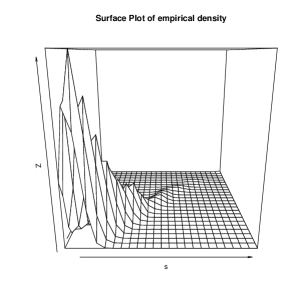
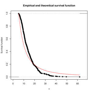
Refer to caption
Figure 5: Surface plot of daily and three-day extreme rainfall.
Refer to caption
Figure 6: Marginal Y1subscript𝑌1Y_{1}.
Refer to caption
Figure 7: Marginal Y2subscript𝑌2Y_{2}.

Now our aim is to compare different well-established bivariate Pareto distributions, namely Mardia’s type I𝐼I bivariate Pareto [24], Bivariate Lomax [23] and MOBVPA [8]. Note that both Mardia’s type I𝐼I and Bivariate Lomax distribution are three-parameter models, whereas both MOBVPA and BB-BVPA are seven-parameter models. From Table 9, based on AIC values, it is clear that our proposed BB-BVPA model fits better than all other models.

Bivariate model Parameters Log-likelihood AIC Mardia’s type I𝐼I [24] σ1=5.2subscript𝜎15.2\sigma_{1}=5.2, σ2=12.1subscript𝜎212.1\sigma_{2}=12.1, α=1.4198𝛼1.4198\alpha=1.4198 -3788.638 7583.277 Bivariate Lomax [23] α1=0.0318subscript𝛼10.0318\alpha_{1}=0.0318, α2=0.0224subscript𝛼20.0224\alpha_{2}=0.0224, θ=2.3303𝜃2.3303\theta=2.3303 -4486.472 8978.943 MOBVPA [8] μ1subscript𝜇1\mu_{1} = 5.25.25.2, μ2subscript𝜇2\mu_{2} = 12.112.112.1, σ1subscript𝜎1\sigma_{1} = 6.47206.47206.4720, σ2subscript𝜎2\sigma_{2} = 5.16605.16605.1660, -2382.115 4778.230 α0subscript𝛼0\alpha_{0} = 0.99080.99080.9908, α1subscript𝛼1\alpha_{1} = 0.25330.25330.2533, α2subscript𝛼2\alpha_{2} = 0.20460.20460.2046 BB-BVPA μ1subscript𝜇1\mu_{1} = 5.25.25.2, μ2subscript𝜇2\mu_{2} = 12.112.112.1, σ1subscript𝜎1\sigma_{1} = 6.27236.27236.2723, σ2subscript𝜎2\sigma_{2} = 5.50595.50595.5059, -1578.189 3170.377 α0subscript𝛼0\alpha_{0} = 2.05892.05892.0589, α1subscript𝛼1\alpha_{1} = 0.00250.00250.0025, α2subscript𝛼2\alpha_{2} = 0.00280.00280.0028

Table 9: MLEs, the log-likelihood and AIC for four different bivariate Pareto distributions.

We wish to estimate the probability of a future landslide using formula (25), i.e., we wish to calculate the probability of a landslide occurring as a consequence of one or three days of extreme precipitation for any given year using the parameter estimates given in last row of Table 9,

P(Y1>39.5Y2>69.9)𝑃subscript𝑌139.5subscript𝑌269.9\displaystyle P(Y_{1}>39.5\cup Y_{2}>69.9)
=1P(Y1>39.5Y2>69.9)absent1𝑃subscript𝑌139.5subscript𝑌269.9\displaystyle=1-P(Y_{1}>39.5\cap Y_{2}>69.9)
=0.0761.absent0.0761\displaystyle=0.0761.

This is higher than the result in Rudvik [33], who analyzed daily, three-day and five-day extreme precipitation amounts from 1913 to 2008 to estimate the yearly risk. From the dataset, it is clear that the number of extreme rainfall that led the landslide over these 100 (1913-2012) years is seven. This result is very close to the seven or eight extreme rainfalls that we would expect based on our model. A clear limitation of this risk estimate calculation is that the thresholds using the equation (25) is not constructed for our particular location. More knowledge about local geological conditions and landslide activity of the specific location may give more precise threshold estimates and hence better risk estimates; it has not been attempted here.

7 Concluding Remarks

We have observed the successful implementation of the EM algorithm for the absolute continuous bivariate Pareto distribution. The approximation process runs in multiple stages. Therefore, the algorithm works better for a moderately larger sample size. Even in the case of three parameters, the estimation procedure is not straightforward. This work also shows some innovative approaches to handle the estimation in the case of location and scale parameters. It has an absolutely continuous probability density function, and we have also studied several properties of this distribution. The model was applied to the rainfall data, where the context dictated that extremes of ordered cumulative data were the object of interest. This work can be further used for the discrimination of several models. The Bayesian estimation of this distribution, even without location and scale parameters using Gamma prior and Reference prior, can also be a challenging problem.

Acknowledgements

The authors would like to thank the Abisko Scientific Research Station, Abisko, Sweden, for providing the precipitation dataset.

Declarations

Data availability The dataset is publicly available and is taken from https://www.polar.se/stoed-till-polarforskning/abisko-naturvetenskapliga-station/.

References

  • Arnold [2015] Barry C. Arnold. Pareto Distributions. CRC Press, 2nd edition, 2015.
  • Arnold and Press [1989] Barry C Arnold and S James Press. Bayesian estimation and prediction for Pareto data. Journal of the American Statistical Association, 84(408):1079–1084, 1989.
  • Arnold et al. [1998] Barry C Arnold, Enrique Castillo, and Jose Maria Sarabia. Bayesian analysis for classical distributions using conditionally specified priors. Sankhyā: The Indian Journal of Statistics, Series B, pages 228–245, 1998.
  • Asimit et al. [2016] Alexandru V Asimit, Edward Furman, and Raluca Vernic. Statistical inference for a new class of multivariate Pareto distributions. Communications in Statistics-Simulation and Computation, 45(2):456–471, 2016.
  • Basu [1971] AP Basu. Bivariate failure rate. Journal of the American Statistical Association, 66(333):103–104, 1971.
  • Block and Basu [1974] Henry W Block and AP Basu. A continuous, bivariate exponential extension. Journal of the American Statistical Association, 69(348):1031–1037, 1974.
  • Coles et al. [2001] Stuart Coles, Joanna Bawa, Lesley Trenner, and Pat Dorazio. An introduction to statistical modeling of extreme values, volume 208. Springer, 2001.
  • Dey and Paul [2018] Arabin Kumar Dey and Biplab Paul. Some Variations of EM Algorithms for Marshall-Olkin Bivariate Pareto Distribution with Location and Scale. Journal of Statistical Theory and Practice, 10, 2018.
  • Dinse [1982] Gregg E Dinse. Nonparametric estimation for partially-complete time and type of failure data. Biometrics, pages 417–431, 1982.
  • Efron and Tibshirani [1994] Bradley Efron and Robert J Tibshirani. An introduction to the bootstrap. CRC press, 1994.
  • Embrechts et al. [2013] Paul Embrechts, Claudia Klüppelberg, and Thomas Mikosch. Modelling extremal events: for insurance and finance, volume 33. Springer Science & Business Media, 2013.
  • Guzzetti et al. [2007] Fausto Guzzetti, Silvia Peruccacci, Mauro Rossi, and Colin P Stark. Rainfall thresholds for the initiation of landslides in central and southern Europe. Meteorology and atmospheric physics, 98(3):239–267, 2007.
  • Hanagal [1996] David D Hanagal. A multivariate Pareto distribution. Communications in Statistics-Theory and Methods, 25(7):1471–1488, 1996.
  • Johnson and Kotz [1975] Norman L Johnson and Samuel Kotz. A vector multivariate hazard rate. Journal of Multivariate Analysis, 5(1):53–66, 1975.
  • Karlin [1968] Samuel Karlin. Total positivity, volume 1. Stanford University Press, 1968.
  • Kotz and Nadarajah [2000] Samuel Kotz and Saralees Nadarajah. Extreme value distributions: theory and applications. world scientific, 2000.
  • Kotz et al. [2004] Samuel Kotz, Narayanaswamy Balakrishnan, and Norman L Johnson. Continuous multivariate distributions, Volume 1: Models and applications, volume 1. John Wiley & Sons, 2004.
  • Kundu and Gupta [2008] Debasis Kundu and Rameshwar D Gupta. Generalized exponential distribution: Bayesian estimations. Computational Statistics & Data Analysis, 52(4):1873–1883, 2008.
  • Kundu and Gupta [2009] Debasis Kundu and Rameshwar D Gupta. Bivariate generalized exponential distribution. Journal of Multivariate Analysis, 100(4):581–593, 2009.
  • Kundu and Gupta [2010] Debasis Kundu and Rameshwar D Gupta. A class of absolutely continuous bivariate distributions. Statistical Methodology, 7(4):464–477, 2010.
  • Kundu and Gupta [2011] Debasis Kundu and Rameshwar D Gupta. Absolute continuous bivariate generalized exponential distribution. AStA Advances in Statistical Analysis, 95(2):169–185, 2011.
  • Kundu et al. [2015] Debasis Kundu, Ankush Kumar, and Arjun K Gupta. Absolute continuous multivariate generalized exponential distribution. Sankhya B, 77(2):175–206, 2015.
  • Lindley and Singpurwalla [1986] Dennis V Lindley and Nozer D Singpurwalla. Multivariate distributions for the life lengths of components of a system sharing a common environment. Journal of Applied Probability, 23(2):418–431, 1986.
  • Mardia [1962] Kanti V Mardia. Multivariate pareto distributions. The Annals of Mathematical Statistics, pages 1008–1015, 1962.
  • Marshall [1996] Albert W Marshall. Copulas, marginals, and joint distributions. Lecture Notes-Monograph Series, pages 213–222, 1996.
  • Marshall and Olkin [1967] Albert W Marshall and Ingram Olkin. A multivariate exponential distribution. Journal of the American Statistical Association, 62(317):30–44, 1967.
  • Mirhosseini et al. [2015] Seyed Mohsen Mirhosseini, Mohammad Amini, D Kundu, and Ali Dolati. On a new absolutely continuous bivariate generalized exponential distribution. Statistical Methods & Applications, 24(1):61–83, 2015.
  • Nanda and Jain [1999] Asok K Nanda and Kanchan Jain. Some weighted distribution results on univariate and bivariate cases. Journal of Statistical planning and Inference, 77(2):169–180, 1999.
  • Nelsen [2007] Roger B Nelsen. An introduction to copulas. Springer Science & Business Media, 2007.
  • Paul et al. [2018] Biplab Paul, Arabin Kumar Dey, and Debasis Kundu. Bayesian analysis of three parameter absolute continuous Marshall-Olkin bivariate Pareto distribution. Communications in Statistics: Case Studies, Data Analysis and Applications, 4:2:57–68, 2018.
  • R Core Team [2022] R Core Team. R: A Language and Environment for Statistical Computing. R Foundation for Statistical Computing, Vienna, Austria, 2022. URL https://www.R-project.org/.
  • Reiss and Thomas [2005] Rolf-Dieter Reiss and Michael Thomas. Statistical Analysis of Extreme Values (for Insurance, Finance, Hydrology and Other Fields). Basel:Birkhäuser, 3rd edition, 2005.
  • Rudvik [2012] Anna Rudvik. Dependence structures in stable mixture models with an application to extreme precipitation. PhD thesis, Chalmers University of Technology, 2012.
  • Vernic [2011] Raluca Vernic. Tail conditional expectation for the multivariate Pareto distribution of the second kind: Another approach. Methodology and Computing in Applied Probability, 13(1):121–137, 2011.