The underlying driver for the C iv Baldwin effect in QSOs with $0<z<5$

Abstract

Broad emission lines is a prominent property of type I quasi-stellar objects (QSOs). The origin of the Baldwin effect for C iv $\lambda 1549~{}$Å broad emission lines, i.e., the luminosity dependence of the C iv equivalent width (EW), is not clearly established. Using a sample of 87 low-$z$ Palomar-Green (PG) QSOs and 126 high-$z$ QSOs across the widest possible ranges of redshift ($0<z<5$), we consistently calculate H$\beta$ -based single-epoch supermassive black hole (SMBH) mass and the Eddington ratio to investigate the underlying driver of the C iv Baldwin effect. An empirical formula to estimate the host fraction in the continuum luminosity at 5100 Å is presented and used in H$\beta$ -based $M_{\rm BH}$ calculation for low-$z$ PG QSOs. It is found that, for low-$z$ PG QSOs, the Eddington ratio has strong correlations with PC1 and PC2 from the principal component analysis, and C iv EW has a strong correlation with the optical Fe ii strength or PC1. Expanding the luminosity range with high-$z$ QSOs, it is found that C iv Baldwin effect exists in our QSOs sample. Using H$\beta$ -based single-epoch SMBH mass for our QSOs sample, it is found that C iv EW has a strong correlation with the Eddington ratio, which is stronger than that with the SMBH mass. It implies that the Eddington ratio seems to be a better underlying parameter than the SMBH mass to drive the C iv Baldwin effect.

1 INTRODUCTION

Broad emission lines is a prominent property of type I active galactic nuclei (AGNs) and quasi-stellar objects (QSOs). It is accepted that these broad emission lines are produced by photoionization in broad-line regions (BLRs) gas, where the accretion disc surround the central supermassive black hole (SMBH) provides the ionizing photos. Baldwin (1977) discovered an anti-correlation between the equivalent width (EW) of the C iv $\lambda 1549~{}$Å emission line and the continuum luminosity in the QSO rest frame, (i.e. the Baldwin effect, see the review by Shields, 2007). Over the past 20 yr, this effect was investigated with different QSOs samples, including other permitted/prohibited emission lines, such as Ly$\alpha$, C iii , Si iv , Mg ii , [O iii] , Fe K$\alpha$ (e.g., Green et al., 2001; Dietrich et al., 2002; Shang et al., 2003; Baskin & Laor, 2004; Xu et al., 2008; Wu et al., 2009; Richards et al., 2011; Bian et al., 2012; Shen & Ho, 2014).

It is believed that the Baldwin effect exists for many UV/optical emission lines. However, its origin is not clearly established. One promising interpretation is the softening of the spectral energy distribution (SED) for increasing luminosity, which lowers the ion populations that having high ionization potentials (e.g., Netzer et al., 1992; Dietrich et al., 2002). Non-isotropic continuum emission and the intrinsic Baldwin effect would provide some of the observed scatter in the Baldwin effect (e.g., Baskin & Laor, 2004). The underlying physical parameters for the Baldwin effect are investigated for many years, such as the eigenvector 1 of Boroson & Green (1992), the Eddington ratio $L_{\rm Bol}/L_{\rm Edd}$ (i.e. the ratio of the bolometric luminosity to the Eddington luminosity), the SMBH mass $M_{\rm BH}$ (e.g., Boroson & Green, 1992; Wills et al., 1999; Boroson, 2002; Shang et al., 2003; Bachev et al., 2004; Baskin & Laor, 2004; Xu et al., 2008; Bian et al., 2012; Shemmer & Lieber, 2015). For a optical-selected sample of Palomar-Green (PG) QSOs, Baskin & Laor (2004) found a strong correlation of the C iv EW with $L_{\rm Bol}/L_{\rm Edd}$ , stronger than that with the continuum luminosity, and suggested that the $L_{\rm Bol}/L_{\rm Edd}$ is the primary physical parameter which drives the C iv Baldwin effect (Shemmer & Lieber, 2015). Using a larger sample of QSOs with $1.5<z<5$ from Sloan Digital Sky Survey (SDSS), Xu et al. (2008) found the C iv EW has a stronger correlation with C iv-based $M_{\rm BH}$ than the $L_{\rm Bol}/L_{\rm Edd}$ . Using C iv-based $M_{\rm BH}$ by Shen et al. (2011) for high-$z$ SDSS QSOs, Bian et al. (2012) also found that there is a correlation between the C iv EW and the C iv -based $M_{\rm BH}$ . However, with Mg ii-based $M_{\rm BH}$ , Bian et al. (2012) found SDSS QSOs in $1.5<z<1.9$ follow the relation found by Baskin & Laor (2004), suggesting the bias in C iv-based $M_{\rm BH}$ .

Due to the larger consumption of telescope time in reverberation mapping (RM), there is about 60 AGN/QSOs with reliable BLRs sizes from RM (Kaspi et al., 2000; Peterson et al., 2004; Du et al., 2016; Shen et al., 2016). From the RM BLRs sizes, there is an empirical R-L relation (Kaspi et al., 2000; Bentz et al., 2013; Du et al., 2015). With this empirical R-L relation, the BLRs size can be derived from the continuum luminosity at 5100 Å. The single-epoch SMBH mass can be calculated from the broad emission lines, such as H$\beta$ , H$\alpha$ , Mg ii , C iv (e.g., Laor, 1998; Bian & Zhao, 2004; Greene & Ho, 2005; Vestergaard & Peterson, 2006; Jun et al., 2015). By the host correction in the continuum luminosity at 5100 Å by Hubble Space Telescope (HST) images for different width slits, Bentz et al. (2013) found that the slope in R-L relation changes from 0.7 to 0.533. It is suggested that C iv -based $M_{\rm BH}$ is biased to the H$\beta$ -based $M_{\rm BH}$ (e.g., Rafiee & Hall, 2011; Shen & Liu, 2012; Bian et al., 2012). For high-$z$ QSOs, the H$\beta$ emission line is shifted to the infrared (IR) band. The IR spectroscopy observation for high-$z$ QSOs is needed to calculate SMBH $M_{\rm BH}$ using the same H$\beta$ emission line as that for low-$z$ QSOs.

In order to investigate the C iv EW relation with the SMBH accretion, we compile a sample of 87 low-$z$ PG QSOs and 126 high-$z$ QSOs across the widest possible ranges of redshift ($0<z<5$) with available spectral information for H$\beta$ $\lambda 4861$ Å and C iv $\lambda 1549$ Å emission lines. Our adopted sample is described in §2, the results and the analysis are given in §3, and the conclusions are presented in §4. All of the cosmological calculations in this paper assume $H_{0}=70\rm{~{}km~{}s^{-1}~{}Mpc^{-1}}$, $\Omega_{M}=0.3$, and $\Omega_{\Lambda}=0.7$.

2 Sample

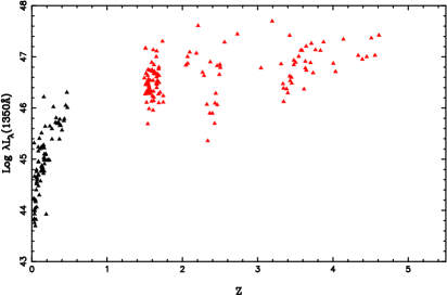
Figure 1: The UV continuous luminosity at 1350Å (in units of erg/s) versus redshift for our low-$z$ and high-$z$ sample. The black triangles denote 87 low-$z$ PG QSOs, and the red triangles denote 126 high-$z$ QSOs.

2.1 low-$z$ sample

The 87 PG QSOs ($0<z<0.5$) are optically selected by a limiting $B$-band magnitude of 16.16, blue $U-B$ colour ($<-0.44$), and dominant starlike appearance, showing broad emission lines classified as type 1 QSOs (Schmidt & Green, 1983; Boroson & Green, 1992). The low-$z$ PG QSOs is representative of bright optically selected QSOs (Jester et al., 2005). It is the most thoroughly explored sample of AGN/QSOs, with a lot of high quality data at most wave bands (e.g., Boroson & Green, 1992; Brandt et al., 2000; Baskin & Laor, 2004; Bian et al., 2014; Shi et al., 2014). Boroson & Green (1992) observed all these 87 PG QSOs with the KPNO 2.1 m telescope and the Gold Spectrograph. The spectra of these objects were made through a $1.5$ arcsec slit with a spectral resolution of about 6.5 Å, covering the range 4300-5700 Å in the rest frame. In this paper, the H$\beta$ width at half-maximum (FWHM) is adopted from Boroson & Green (1992) used in the H$\beta$ -based single epoch SMBH mass calculation (see also Boroson, 2002; Vestergaard & Peterson, 2006). In Table 1, the spectral-resolution-corrected H$\beta$ FWHM adopted from Vestergaard & Peterson (2006) is listed in Col. (9). For UV spectra of these 87 PG QSOs, Baskin & Laor (2004) obtained archived UV spectra for these 85 PG QSOs, 47 from the HST and 38 from the International Ultraviolet Explorer (IUE). For three of them (PG 0934+013, PG 1004+130, PG 1448+273), their UV archival spectra did not have a sufficient S/N to measure the C iv EW, and PG 1700+518 is a broad-absorption line (BAL) QSOs. In addition, there are five BAL QSOs and 16 radio-loud (RL) QSOs. The continuum luminosity at 1350 Å / 5100 Å is calculated from the (SED) presented by Neugebauer et al. (1987) (Baskin & Laor, 2004; Vestergaard & Peterson, 2006). Table 1 lists the information of 87 PG QSOs. Fig. 1 shows $\lambda L_{\lambda}(1350\AA)$ versus $z$, where black triangles denote 87 PG QSOs.

2.2 High-$z$ sample

In this paper, the H$\beta$ emission line is needed to calculate the single-epoch $M_{\rm BH}$ for all QSOs and to investigate the underlying parameter for the C iv Baldwin effect. For high-$z$ QSOs with available C iv $\lambda 1459$ Å observed by ground telescope ($z>1.5$), the H$\beta$ emission line is shifted to the IR band.

Shen & Liu (2012) presented 60 intermediate-redshift QSOs ($z\sim 1.5-2.2$) selected from SDSS DR7. Their near-IR spectrum are observed with TripleSpec (Wilson et al., 2004) ($0.95-2.46~{}\mu m$) on the ARC 3.5 m telescope, and with the Folded-port InfraRed Echellette (Simcoe et al., 2010) ($0.8-2.5~{}\mu m$) on the 6.5 m Magellan-Baade telescope. With TripleSpec, the total exposure is typically $1-1.5$ hr with slits widths of both 1.1″ and 1.5″, and the resulting spectral resolution of $R\sim 2500-3500$. With FIRE, typical total exposure times were 45 min with the slit width of 0.6″. The spectral resolution is $R\sim 6000$ (50 ${\rm km\,s^{-1}}$). They performed standard ABBA dither patterns to aid sky subtraction and observed a nearby A0V star as flux and telluric standard. Jun et al. (2015) presented near-Infrared grism spectra for 155 QSOs ($3.3<z<6.4$) from the $AKARI$ space telescope. It is composed of optically luminous and spectroscopically confirmed type 1 QSOs at $z>3$, mostly out of SDSS DR5. The spectrum coverage is $2.5-5.0~{}\mu m$. The spectral resolution is $R=120$ at $3.6\mu m$, corresponding to a velocity resolution of 2500 km s^-1 . Jun et al. (2015) gave 43 high-$z$ QSOs with H$\alpha$ information. From above two literatures and others (Shemmer et al., 2004; Netzer et al., 2007; Dietrich et al., 2009; Assef et la., 2011; Ho et al., 2012; Shen & Liu, 2012; Jun et al., 2015; Shemmer & Lieber, 2015), we assembled a sample of 182 high-$z$ QSOs with H$\beta$ /H$\alpha$ data.

In order to obtain the UV C iv data for these high-$z$ QSOs, we search their SDSS spectral data. The SDSS used a 2.5-m wide-field telescope at Apache Point Observatory near Sacramento Peak in Southern New Mexico to conduct an imaging and spectroscopic survey. Shen et al. (2011) presented a compilation of properties of the 105,783 QSOs in the SDSS DR7 catalogue, where they used multi-Gaussians to fit the main emission lines, such as C iv , Mg ii , H$\beta$ , H$\alpha$ depending on the redshift. We search these 182 high-$z$ QSOs in the SDSS DR7 QSOs sample by Shen et al. (2011), and obtain 126 high-$z$ QSOs with C iv fitting data and the luminosity at 1350 Å. Shen et al. (2011) suggested that measurements of C iv EW for most objects are unbiased to within 20% down to S/N $\sim 3$. For our SDSS high-z sample, their S/N are larger than 3. There are 7 BAL QSOs, 12 RL QSOs, 11 weak line QSOs ($\rm EW(CIV)<10\AA$). For these 126 high-$z$ QSOs, we respectively select 10, 15, 7, 1, 60, 7, and 26 high-$z$ QSOs from the literatures of Shemmer et al. (2004); Netzer et al. (2007); Assef et la. (2011); Ho et al. (2012); Shen & Liu (2012); Shemmer & Lieber (2015); Jun et al. (2015). For 26 high-$z$ QSOs in Jun et al. (2015), we obtain the $\lambda L_{\lambda}(5100\AA)$ and H$\alpha$ FWHM from table 7 in Jun et al. (2015). We convert the H$\alpha$ FWHM to H$\beta$ FWHM by the formula (Jun et al., 2015),

$$\rm log~{}\frac{FWHM(H\beta)}{1000~{}{\rm km\ s}^{-1}})=(1.061\pm 0.013)log~{}\frac{FWHM(H\alpha)}{1000~{}{\rm km\ s}^{-1}}\,$$

$$+(0.055\pm 0.008).$$ (1)

The FWHM of H$\alpha$ or H$\beta$ is listed in Col. (7) in Table 2. These 126 high-$z$ QSOs are used as our final high-$z$ QSOs sample with available H$\beta$ and C iv data at the same time. It is larger than the high-$z$ sample of 36 QSOs ($z<3.5$) by Shemmer & Lieber (2015). Our sample covers the redshift of $0<z<5$ and the $log\lambda L_{\lambda}(1350\AA)$ of $43.6-47.7$. Table 2 lists the properties of high-z QSOs. In Fig. 1, the red triangles denote these 126 high-$z$ QSOs.

3 Result and Discussion

3.1 The host contribution in the continuum luminosity at 5100 Å

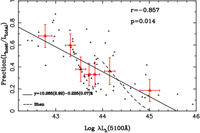
Figure 2: The host fraction in the total continuum luminosity at 5100 Å versus the total continuum luminosity at 5100 Å. The black triangles are the observation data from (Bentz et al., 2013), the red triangle denotes the value of each bin. The black solid line is the best fit for bin data. The dotted line is the formula from (Shen et al., 2011). For red bin data, the Spearman correlation coefficient and the probability of the null hypothesis are shown in the panel.

With the empirical R-L relation, the BLRs size can be derived from the nuclei continuum luminosity. Based on the stacked SDSS spectra, Shen et al. (2011) gave an empirical formula to give the ratio of host to nuclei QSOs luminosity for the total QSOs continuum luminosity of $log(\lambda L_{\lambda}(5100\AA)/erg~{}s^{-1})=44.1-45.5$. When total QSOs luminosity are larger than $10^{45}erg/s$, the host contribution is negligible. For high-$z$ QSOs in our sample, we found they are all $log(\lambda L_{\lambda}(5100\AA)/erg~{}s^{-1})>45$, and the host contamination is generally negligible. For low-$z$ PG QSOs, we need to correct the host contribution to derive the BLRs sizes because of their lower luminosity at 5100Å.

Using GALFIT (Peng et al., 2002) to model HST host-galaxy images of 41 RM AGN Bentz et al. (2013) did the host correction for 71 observation data at 5100 Å. For the host fraction in the total continuum luminosity from (Bentz et al., 2013), we bin the observation data into seven bins according the total continuum luminosity at 5100 Å. The value of each bin is the average of total continuum luminosity and the host fraction, and the error of each bin value is the standard deviation. For the bin data, the Spearman correlation test gives the Spearman correlation coefficient $r_{s}=0.86$ and the probability of the null hypothesis $P_{\rm null}=1.4\times 10^{-2}$. The relationship is derived by using algorithms FITEXY (Press et al., 1992).

$$f=(10.265\pm 2.92)-(0.225\pm 0.07)~{}log\lambda L_{\lambda}(5100\AA)^{total}$$ (2)

where $f$ is the host fraction in the total continuum luminosity at 5100 Å, $\lambda L_{\lambda}(5100\AA)^{total}$ is the total continuum luminosity at 5100 Å. In Fig.  2, we also show the host fraction formula of Shen et al. (2011) for SDSS fibre, which is consistent with our formula, considering the decreasing tendency with large $\lambda L_{\lambda}(5100\AA)$ . The host fraction decreases from about 80% at $\lambda L_{\lambda}(5100\AA)=10^{42}erg/s$ to about 10% at $\lambda L_{\lambda}(5100\AA)=10^{45}erg/s$.

For 87 low-$z$ PG QSOs, there are 16 RM objects, where the host fractions are adopted from Bentz et al. (2013). For other PG QSOs with the total continuum luminosity $\lambda L_{\lambda}(5100\AA)$ below $10^{45.5}erg/s$, we use our formula to correct the host contribution. The host-corrected $\lambda L_{\lambda}(5100\AA)$ is listed in Col. (8) in Table 1. Fig.  3 shows the distribution of total luminosity at 5100 Å (top panel) for 87 PG QSOs and the distribution of the difference between the total continuum luminosity and the nuclei continuum luminosity at 5100 Å in logarithm, i.e., $log(1/(1-f))$ (bottom panel). Considering the range of log $\lambda L_{\lambda}(5100\AA)$ of $43.6-46.2$, the host fraction $f$ in the total luminosity at 5100Å is estimated to be less than about 50% from our formula of Eq.  2. $log(1/(1-f))=0.3$ for $f=50\%$ (bottom panel in Fig.  3).

Figure 3: Top: distribution of total continuum luminosity at 5100 Å. Bottom: distribution of the difference between the total continuum luminosity and the nuclei continuum luminosity at 5100 Å in logarithm, i.e., $log(1/(1-f))$.

3.2 $M_{\rm BH}$ and $L_{\rm Bol}/L_{\rm Edd}$ 

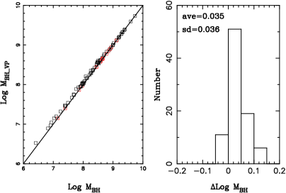
Figure 4: Left: $M_{\rm BH}$ given in (Vestergaard & Peterson, 2006) versus our calculated $M_{\rm BH}$ considering host contribution for 87 low-$z$ PG QSOs. The red square denotes 16 RM objects. The black line is 1:1. Right: distribution of the $M_{\rm BH}$ difference.

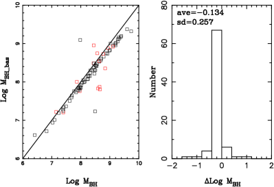
Figure 5: Left: $M_{\rm BH}$ given in (Baskin & Laor, 2004) versus our calculated $M_{\rm BH}$ considering host contribution for 87 low-$z$ PG QSOs. The red square denotes 16 RM objects. The black line is 1:1. Right: distribution of the $M_{\rm BH}$ difference.

Using 32 RM SMBHs masses from Peterson et al. (2004), Vestergaard & Peterson (2006) gave a formula to calculate the SMBH mass from the AGN/QSOs single-epoch spectrum, where H$\beta$ FWHM and the continuum luminosity at 5100 Å are measured.

$${logM_{\rm BH}(H\beta)}=log\{(\frac{\rm FWHM(H\beta)}{1000~{}{\rm km\ s}^{-1}})^{2}\times(\frac{\rm\lambda L_{\lambda}(5100\AA)}{10^{44}~{}{\rm erg\ s}^{-1}})^{0.5}\}\,$$

$$+(6.91\pm 0.02)$$ (3)

With above formula, we calculate the black hole mass using FWHM(H$\beta$ ) and host-corrected continuum luminosity at 5100 Å for 71 non-RM low-$z$ PG QSOs and 126 high-$z$ QSOs (see Tables 1 and 2). The host-corrected $M_{\rm BH}$ is listed in Col. (10) in Table 1 for low-z PG QSOs. We also list the $M_{\rm BH}$ given by Vestergaard & Peterson (2006) in Col. (11) and that by Baskin & Laor (2004) in Col. (12) in Table 1. Fig.  4 shows $M_{\rm BH}$ given in Vestergaard & Peterson (2006) (without host correction, same formula) versus our calculated $M_{\rm BH}$ considering host correction for 87 low-$z$ PG QSOs (left-hand panel) and the distribution of their $M_{\rm BH}$ difference (right-band panel). The red squares denote RM objects. The mean value of their difference is 0.035 with the standard deviation of 0.036. Considering that $M_{\rm BH}\propto L^{0.5}$, the log$\lambda L_{\lambda}(5100\AA)$ correction of 0.1 dex would lead to a decrease of 0.05 dex, which is consistent with the result in Fig.  4. With a different formula by Laor (1998), Baskin & Laor (2004) also calculated the $M_{\rm BH}$ for 87 PG QSOs. Fig.  5 shows our calculated $M_{\rm BH}$ versus that in Baskin & Laor (2004) (left-hand panel) and the distribution of their difference (right-hand panel). The mean value of their difference is 0.134 dex with the standard deviation of 0.257. Considering intrinsic scatter in $M_{\rm BH}$ calculation of about 0.3 dex (e.g., Shen et al., 2011), the host correction in $M_{\rm BH}$ calculation is negligible for low-$z$ PG QSOs sample, although it is important for low-luminosity AGN/QSOs. For high-z QSos, the $M_{\rm BH}$ is also listed in Col. (9) in Table 2.

We use the nuclei continuum luminosity at 5100Å to calculate the bolometric luminosity by a bolometric correction of 9.26 (Richards et al., 2006), and then calculate the Eddington ratio $L_{\rm Bol}/L_{\rm Edd}$ for our low-$z$ QSOs. For high-$z$ QSOs, $\lambda L_{\lambda}(5100\AA)$ is so large that the host contribution can be neglected, and $L_{\rm Bol}/L_{\rm Edd}$ are calculated as that for low-$z$ PG QSOs. $L_{\rm Bol}/L_{\rm Edd}$ for high-$z$ QSOs is listed in Col. (10) in Table 2.

3.3 The relation between the SMBH accretion and PC1/PC2 from PCA

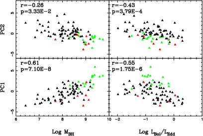
Figure 6: Left: the relationship between $M_{\rm BH}$ and PC1, PC2. Right: the relationship between Eddington ratio $L_{\rm Bol}/L_{\rm Edd}$ and PC1, PC2. Green triangles denote RL QSOs. Red triangles denote BAL QSOs. The Spearman correlation coefficient and the probability of the null hypothesis is shown in the left in each panel.

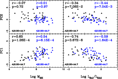
Figure 7: The same as Fig.  6  but for two subsamples dividing by luminosity $log\lambda L_{\lambda}(5100\AA)=44.7$ (excluding RL QSOs and BAL QSOs). The back triangles denote PG QSOs with smaller $\lambda L_{\lambda}(5100\AA)$ and blue triangles denote PG QSOs with larger $\lambda L_{\lambda}(5100\AA)$ . The Spearman correlation coefficient and the probability of the null hypothesis is shown in each panel.

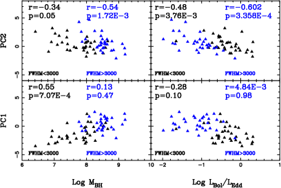
Figure 8: Same as Fig.  6  but for two subsamples dividing by $FWHM(H\beta)=3000{\rm km\ s}^{-1}$ (excluding RL QSOs and BAL QSOs). The back triangles denote PG QSOs with smaller H$\beta$ FWHM and blue triangles denote PG QSOs with larger H$\beta$ FWHM. The Spearman correlation coefficient and the probability of the null hypothesis is shown in each panel.

With the optical spectral information and additional information from other bands for 87 low-$z$ PG QSOs, Boroson & Green (1992) presented principal component analysis (PCA) and found that the variance in the optical emission lines and the continuum (radio through X-ray) was mostly contained in two sets of correlations, eigenvectors of the correlation matrix. Principal component 1 (PC1) links the strength of optical Fe ii emission, [O iii] emission, and H$\beta$ line asymmetry. Principal component 2 (PC2) involves optical luminosity and the strength of He ii 4686 and $\alpha_{\rm ox}$. With the single-epoch SMBH mass derived from H$\beta$ (Kaspi et al., 2000), Boroson (2002) found that PC1 is mainly correlation with $L_{\rm Bol}/L_{\rm Edd}$ and PC2 has a strong correlations with $M_{\rm BH}$ and $L_{\rm Bol}/L_{\rm Edd}$ . He suggested that PC1 is driven predominantly by the Eddington ratio, and PC2 is driven by the accretion rate. The coefficient listed in table 1 in Boroson (2002) is used to calculate the PC1/PC2 values. PC1/PC2 values are listed in Col. (15-16) in Table 1. Fig.  6 shows PC1/PC2 versus our calculated $M_{\rm BH}$ and $L_{\rm Bol}/L_{\rm Edd}$ for 87 low-$z$ PG QSOs. We find that PC1 has strong correlations with $M_{\rm BH}$ and $L_{\rm Bol}/L_{\rm Edd}$ , r=0.66, -0.46, respectively. PC2 has a strong correlation with $M_{\rm BH}$ and a weak correlation with $L_{\rm Bol}/L_{\rm Edd}$ , r=-0.53, -0.34, respectively. These results are consistent with Boroson (2002). In Fig.  6, we also show 16 RL QSOs (green triangle) and 5 BAL QSOs (red triangle). Considering the speciality RL QSOs and BAL QSOs, we exclude them and find that PC1 still has strong correlation with $M_{\rm BH}$ and $L_{\rm Bol}/L_{\rm Edd}$ , r=0.61, -0.55, respectively. PC2 has a weak correlation with $M_{\rm BH}$ and a strong correlation with $L_{\rm Bol}/L_{\rm Edd}$ , r=-0.26, -0.43, respectively. It is different to the results by Boroson (2002), where PC2 has a very weak correlation with $L_{\rm Bol}/L_{\rm Edd}$ and a strong correlation with $M_{\rm BH}$ . With our calculated $M_{\rm BH}$ and $L_{\rm Bol}/L_{\rm Edd}$ and excluding RL QSO ang BAL QSO, we find that PC2 has a strong correlation with $L_{\rm Bol}/L_{\rm Edd}$ and a weak correlation with $M_{\rm BH}$ . We think it is due to narrower PC1/PC2 parameter space (see Fig.  6).

In Fig.  7, we divide low-$z$ PG QSOs into two parts at $log\lambda L_{\lambda}(5100\AA)=44.7$. For low-luminosity part, PC1 has strong correlations with $M_{\rm BH}$ and $L_{\rm Bol}/L_{\rm Edd}$ . PC2 has weak correlations with $M_{\rm BH}$ and $L_{\rm Bol}/L_{\rm Edd}$ . For high-luminosity part, PC1 still has strong correlations with $M_{\rm BH}$ and $L_{\rm Bol}/L_{\rm Edd}$ . PC2 has a weak correlation with $M_{\rm BH}$ and a strong correlation with $L_{\rm Bol}/L_{\rm Edd}$ . We find that there is no correlation between $M_{\rm BH}$ and PC2 no matter at low luminosity or high luminosity. It is suggested that there exists the BLRs orientation effect to derive the BLR velocity from FWHM (Shen & Ho, 2014). In Fig.  8, we divide low-$z$ PG QSOs into two parts at $\rm FWHM(H\beta)=3000~{}{\rm km\ s}^{-1}$. For low-FWHM part, PC1 has a strong correlation with $M_{\rm BH}$ and a weak correlation with $L_{\rm Bol}/L_{\rm Edd}$ . PC2 has weak correlations with $M_{\rm BH}$ and $L_{\rm Bol}/L_{\rm Edd}$ . For high-FWHM part, PC1 still has very weak correlations with $M_{\rm BH}$ and $L_{\rm Bol}/L_{\rm Edd}$ . PC2 has strong correlations with $M_{\rm BH}$ and $L_{\rm Bol}/L_{\rm Edd}$ . The dividing with FWHM affects seriously the correlations between PC1 and $M_{\rm BH}$ and $L_{\rm Bol}/L_{\rm Edd}$ . Because PC1 has a strong correlation with H$\beta$ FWHM, dividing PG QSOs based on H$\beta$ FWHM would lead to narrower PC1 parameter space, which would lead to weaken PC1 correlation with $M_{\rm BH}$ and $L_{\rm Bol}/L_{\rm Edd}$ . PC2 also has a strong correlation with continuum luminosity, dividing PG QSOs based on the luminosity would lead to narrower PC2 parameter space, which would lead to weaken PC2 correlation with $M_{\rm BH}$ and $L_{\rm Bol}/L_{\rm Edd}$ . Therefore, considering the PG QSOs subsample with different radio loudness, continuum luminosity, and H$\beta$ FWHM, the narameter range limitation will change the strongness of the relations between PC1/PC2 and $M_{\rm BH}$ , $L_{\rm Bol}/L_{\rm Edd}$ . Large sample with larger parameter coverage is needed for this kind of work in the future.

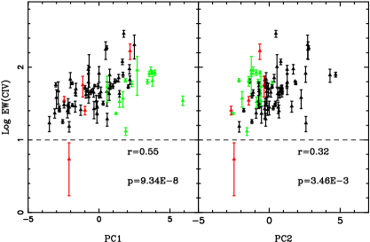
Figure 9: Left: the relationship between C iv EW and PC1. Right: the relationship between C iv EW and PC2. The marks are the same as Fig. 6

Since PC1/PC2 has a correlation with $M_{\rm BH}$ or $L_{\rm Bol}/L_{\rm Edd}$ , in Fig.  9, we show the relationship between C iv EW and PC1/PC2. The C iv EW has a strong correlation with PC1 and the correlation with PC2 is a little weaker. Excluding RL QSOs and BAL QSOs, these correlations become stronger. From PCA shown in Boroson (2002), PC1 has a strong correlation with the Fe ii strength, $R_{\rm Fe}$ (the ratio of optical Fe ii and H$\beta$ EW). We find C iv EW also has a strong correlation with $R_{\rm Fe}$ with $r=-0.59$.

3.4 Physical driver of the Baldwin effect of C iv 

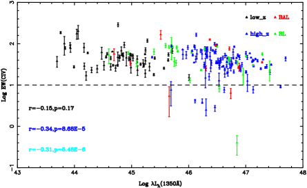
Figure 10: The C iv Baldwin effect, i.e., the C iv EW versus the UV continuous luminosity at 1350Å for our sample of low-$z$ and high-$z$ QSOs. Black triangles denote 81 PG QSOs with low redshift ($z<0.5$), and blue triangles denote SDSS QSOs ($1.5<z<5$). Red triangles denote BAL QSOs and green triangles denote RL QSOs.

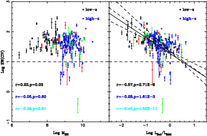
Figure 11: Left: the relationship between C iv EW and $M_{\rm BH}$ . Right: the relationship between C iv EW and $L_{\rm Bol}/L_{\rm Edd}$ . The marks are the same as Fig. 10. The solid line is the best linear fitting of BCES bisector for the low-$z$ sample. The dotted lines are the best fitting of BCES bisector for the entire sample with $2\sigma$. BAL QSOs, RL QSOs and weak line QSOs are excluded from the entire sample during the fitting.

For low-$z$ PG QSOs, Baskin & Laor (2004) found that the C iv Baldwin effect is weak. Fig.  10 shows the C iv Baldwin effect for our low-$z$ and high-$z$ QSOs sample. For the 81 low-$z$ PG QSOs subsample, the C iv Baldwin effect is weak, with $r=-0.15$. It is consistent with the result by Baskin & Laor (2004). Considering the speciality of RL QSOs and BAL QSOs, we exclude 16 RL QSOs and 5 BAL QSOs, and find that the C iv Baldwin effect becomes stronger with $r=-0.25$. For high-$z$ QSOs subsample, the C iv Baldwin effect is stronger than low-$z$ PG QSOs subsample with $r=-0.34$. Excluding 12 RL QSOs, 7 BAL QSOs and 11 weak line QSOs in high-$z$ subsample, the C iv Baldwin effect becomes stronger with $r=-0.45$. For the total sample, we find there exists a C iv Baldwin effect with $r=-0.3$, which is consistent with the result by Bian et al. (2012) from 35019 QSOs in SDSS DR7. We notice that, for the total sample, excluding RL QSOs, BAL QSOs, and weak line QSOs, the correlation coefficient in C iv Baldwin effect doesn’t increase.

For the high-$z$, we calculate the SMBH $M_{\rm BH}$ and $L_{\rm Bol}/L_{\rm Edd}$ using the same H$\beta$ emission line as that for low-$z$ PG QSOs. Fig.  11 shows C iv EW versus $M_{\rm BH}$ (left-hand panel) and $L_{\rm Bol}/L_{\rm Edd}$ (right-hand panel). For low-$z$ PG QSOs subsample, there is a weak correlation between C iv EW and $M_{\rm BH}$ with $r=-0.23$ and $P_{\rm null}=0.03$. However, for high-$z$ QSOs subsample or the total sample, the correlations become weaker with $r=-0.05$, $P_{\rm null}=0.60$ and $r=-0.09$, $P_{\rm null}=0.21$, respectively. For low-$z$ PG QSOs subsample, C iv EW has a strong correlation with $L_{\rm Bol}/L_{\rm Edd}$ with $r=-0.57$, which is consistent with the result by (Baskin & Laor, 2004). For the high-$z$ subsample, the relation becomes weaker with r=-0.28. For the total sample, C iv EW has a strong correlation with $r=-0.45$, $P_{\rm null}=1.52\times 10^{-11}$. The correlation still exists when excluding RL QSOs, BAL QSOs and weak line QSOs. For the relation between C iv EW and $L_{\rm Bol}$(i.e., $\lambda L_{\lambda}(5100\AA)$ ), we find r=-0.15, -0.23, -0.27 for low-$z$, high-$z$, total sample, respectively. Considering that the correlation between C iv EW and $L_{\rm Bol}/L_{\rm Edd}$ is stronger than the relation between C iv EW and $M_{\rm BH}$ , and the C iv Baldwin effect, the Eddington ratio seems to be a better underlying physical parameter than the central SMBH $M_{\rm BH}$ in C iv Baldwin effect. Considering intrinsic scatter of 0.3 dex in $L_{\rm Bol}/L_{\rm Edd}$ , we use the bivariate correlated errors and scatter method (BCES; Akritas et la., 1996) to perform the linear regression (Table. 3). The BCES Bisector best-fitting relation for low-$z$ PG QSOs subsample is,

$$\rm log~{}EW(C~{}IV)=(-0.53\pm 0.10)log(\lambda L_{\lambda}(5100\AA))\,$$

$$+(1.28\pm 0.08)$$ (4)

is plotted as the solid line in Fig.  11. The high-$z$ QSOs follow the solid line found in low-$z$ PG QSOs subsample. Some of weak line QSOs deviated from the above fitting line. Considering the contamination in C iv EW measurement for BAL QSOs, and the jet effect in mass calculation for RL QSOs, we exclude RL QSOs, BAL QSOs and weak line QSOs, a new BCES Bisector best-fitting relation for the total QSOs sample is,

$$\rm log~{}EW(C~{}IV)=(-0.58\pm 0.09)log(\lambda L_{\lambda}(5100\AA))\,$$

$$+(1.35\pm 0.05)$$ (5)

is plotted as the dash lines with $2\sigma$ in the slope in Fig.  11. It is consistent with the result by Shemmer & Lieber (2015). The slope of -0.56 is steeper than the slope of -0.268 found by Bian et al. (2012) with the Mg ii -based $L_{\rm Bol}/L_{\rm Edd}$ . For RL QSOs, BAL QSOs and weak line QSOs, the C iv Baldwin effect, as well as the $L_{\rm Bol}/L_{\rm Edd}$ origin, need to be investigated in larger sample with reliable C iv EW, the UV continuum luminosity, $M_{\rm BH}$ and $L_{\rm Bol}/L_{\rm Edd}$ .

4 Conclusions

We compile a sample of 87 low-$z$ and 126 high-$z$ QSOs across the widest possible ranges of redshift ($0<z<5$) with available H$\beta$ and C iv observations. The H$\beta$ -based single-epoch SMBH $M_{\rm BH}$ and $L_{\rm Bol}/L_{\rm Edd}$ are consistently calculated for QSOs from low-$z$ to high-$z$, which is used to investigate the underlying driver for the C iv Baldwin effect. The main conclusions can be summarized as follows.

(1) An empirical formula is presented to estimate the host correction in the continuum luminosity at 5100Å. For low-$z$ PG QSOs, the estimated host fraction is less than 50%. For 87 low-$z$ and 126 high-$z$ QSOs, the H$\beta$ -based single-epoch SMBH $M_{\rm BH}$ and $L_{\rm Bol}/L_{\rm Edd}$ are consistently calculated.

(2) Considering PC1/PC2 from optical PCA, it is found that PC1 has strong correlations with $M_{\rm BH}$ and $L_{\rm Bol}/L_{\rm Edd}$ . PC2 has a strong correlation with $M_{\rm BH}$ and a weak correlation with $L_{\rm Bol}/L_{\rm Edd}$ . It suggests that $L_{\rm Bol}/L_{\rm Edd}$ is the main driver of PC1, which is consistent with Boroson (2002). For low-$z$ PG QSOs, C iv EW has a relatively weak correlation with the continuum luminosity at 1350 Å. The C iv EW has a strong correlation with the optical Fe ii strength or PC1.

(3) For low-$z$ PG QSOs subsample, excluding the RL QSOs and BAL QSOs, the C iv Baldwin effect becomes stronger. For low-$z$ and high-$z$ sample, there exists a C iv Baldwin effect with $r=-0.3$, which is consistent with the result by Bian et al. (2012) from 35019 QSOs in SDSS DR7. For the total sample, the correlation between C iv EW and H$\beta$ -based $M_{\rm BH}$ is very weak, and C iv EW has a strong correlation with $L_{\rm Bol}/L_{\rm Edd}$ . The Eddington ratio seems to be a better underlying physical parameter than the SMBH $M_{\rm BH}$ in C iv Baldwin effect. For RL QSOs, BAL QSOs and weak line QSOs, the C iv Baldwin effect, as well as the $L_{\rm Bol}/L_{\rm Edd}$ origin, need to be investigated in larger sample.

5 ACKNOWLEDGEMENTS

We are very grateful to the anonymous referee for her/his instructive comments which improved the content of the paper. This work has been supported by the National Science Foundations of China (Nos. 11373024, 11173016 and 11233003).

Table 1: The properties of 87 PG QSOs. Col.(1): Sequence number; Col.(2): Name of PG QSOs, and the superscript of ^a in the Col. (2) indicates the reverberation mapping objects; Col.(3): Redshift from (Schmidt & Green, 1983); Col.(4): The continuum luminosity at 1350Å in units of erg/s (in logarithm scale); Col.(5): The equivalent widths of C iv in units of Å; Col.(6): The ratio of the equivalent widths of Fe ii (4434-4684Å) and H$\beta$ ; Col.(7-8): The continuum luminosity at 5100 Å (Vestergaard & Peterson, 2006; Neugebauer et al., 1987; Schmidt & Green, 1983) and the host corrected luminosity at 5100Å, in units of erg/s (in logarithm scale); Col.(8): The host corrected continuum luminosity at 5100 Å, in units of erg/s (in logarithm scale); Col.(9): The H$\beta$ FWHM in units of km s^-1 (Vestergaard & Peterson, 2006); Col.(10, 11, 12): The host-corrected $M_{\rm BH}$ in this work (all in logarithm scale), the $M_{\rm BH}$ from other works (Vestergaard & Peterson, 2006; Baskin & Laor, 2004); Col.(13): The host-corrected Eddington ratio (in logarithm scale); Col.(14): The radio loudness (in logarithm scale); Col.(15, 16): Eigenvector 1 and Eigenvector 2 of optical PCA.

N Name $z$ $L_{1350}$ EW(C IV) $R_{\rm FeII}$ $L_{5100}$ $L_{5100,cor}$ FWHM_Hβ $M_{\rm BH,cor}$ $M_{\rm BH,VP}$ $M_{\rm BH,BL}$ $L_{\rm Bol}/L_{\rm Edd}$ $R$ $pc1$ $pc2$ (erg s^-1 ) (Å) (erg s^-1 ) (erg s^-1 ) (km s^-1 ) ($M_{\odot})$ ($M_{\odot})$ ($M_{\odot}$) (1) (2) (3) (4) (5) (6) (7) (8) (9) (10) (11) (12) (13) (14) (15) (16) 1 0003+158 0.450 46.050 $63.5\pm{4.6}$ 0.00 46.018 46.018 4750.7 9.273 9.273 9.055 -0.388 2.24 3.409 -0.796 2 $0003+199^{a}$ 0.025 44.232 $60.1\pm{2.6}$ 0.62 44.160 43.720 1585.0 7.152 7.152 7.220 -0.566 -0.57 -1.896 1.860 3 0007+106 0.089 44.943 $59.0\pm{5}$ 0.35 44.816 44.734 5084.6 8.689 8.731 8.561 -1.089 2.29 2.302 0.188 4 $0026+129^{a}$ 0.142 45.240 $19.3\pm{3.9}$ 0.51 45.100 44.910 1821.0 8.594 8.594 7.833 -0.818 0.03 0.574 -0.248 5 0043+039 0.384 45.658 $5.4\pm{3.7}$ 1.18 45.537 45.537 5290.8 9.126 9.126 8.952 -0.722 -0.92 -2.112 -2.484 6 0049+171 0.064 44.064 $203.0\pm{73}$ 0.00 44.004 43.813 5234.3 8.254 8.350 8.146 -1.575 -0.49 2.492 2.700 7 0050+124 0.061 44.755 $29.9\pm{1.5}$ 1.47 44.794 44.709 1171.4 7.402 7.444 7.238 0.173 -0.48 -2.163 -0.627 8 $0052+251^{a}$ 0.155 45.277 $119.0\pm{10.5}$ 0.23 45.030 44.750 5187.0 8.567 8.567 8.745 -0.951 -0.62 1.649 0.816 9 0157+001 0.164 45.099 $43.0\pm{8}$ 0.71 44.975 44.911 2431.9 8.137 8.169 8.006 -0.360 0.33 0.718 0.594 10 $0804+761^{a}$ 0.100 45.406 $45.0\pm{3}$ 0.67 45.060 44.850 3045.0 8.841 8.841 8.352 -1.125 -0.22 -0.593 -0.651 11 0838+770 0.131 44.852 $50.0\pm{10}$ 0.89 44.727 44.634 2763.8 8.110 8.157 7.992 -0.610 -0.96 -1.628 -0.060 12 $0844+349^{a}$ 0.064 44.634 $28.0\pm{5}$ 0.89 44.490 44.367 2386.0 7.966 7.966 7.759 -0.733 -1.52 -2.101 0.629 13 $0921+525^{a}$ 0.035 43.758 $186.0\pm{11}$ 0.14 43.630 43.590 2079.0 7.400 7.400 7.206 -0.944 0.17 0.539 2.775 14 0923+129 0.190 43.923 $93.0\pm{13}$ 0.53 43.860 43.647 7598.4 8.495 8.601 7.233 -1.982 -0.85 -0.756 1.260 15 0923+201 0.029 45.314 $28.0\pm{6}$ 0.72 45.038 44.981 1956.7 7.984 8.012 9.094 -0.136 0.32 -0.129 -0.003 16 0934+013 0.050 – $-$ 0.48 43.875 43.664 1254.3 6.939 7.044 – -0.409 -0.42 -0.838 3.188 17 0947+396 0.206 44.975 $55.0\pm{4}$ 0.23 44.808 44.725 4816.7 8.638 8.679 8.530 -1.047 -0.60 0.981 1.244 18 $0953+414^{a}$ 0.239 45.646 $54.9\pm{5}$ 0.25 45.400 45.130 3111.0 8.441 8.441 8.488 -0.445 -0.36 0.800 -0.734 19 1001+054 0.161 44.979 $34.9\pm{4.6}$ 0.82 44.741 44.650 1699.8 7.696 7.741 7.645 -0.180 -0.30 -2.452 -1.449 20 1004+130 0.240 – $-$ 0.23 45.536 45.536 6290.4 9.275 9.275 – -0.873 2.36 0.818 -3.485 21 1011-040 0.058 44.398 $25.0\pm{5}$ 0.73 44.259 44.105 1381.0 7.243 7.320 7.190 -0.272 -1.00 -2.225 0.682 22 1012+008 0.185 45.104 $23.0\pm{6}$ 0.66 45.011 44.951 2614.7 8.220 8.250 8.069 -0.403 -0.30 -0.145 -0.549 23 1022+519 0.045 43.694 $38.0\pm{11}$ 1.08 43.696 43.456 1566.4 7.028 7.148 6.940 -0.706 -0.64 -3.002 2.245 24 1048-090 0.344 45.697 $91.0\pm{50}$ 0.09 45.596 45.596 5610.8 9.206 9.206 9.022 -0.744 -1.00 2.683 -1.268 25 1048+342 0.167 44.908 $46.0\pm{17}$ 0.32 44.708 44.613 3580.9 8.324 8.372 8.241 -0.845 2.58 0.559 -0.192 26 1049-005 0.357 45.713 $67.0\pm{8.8}$ 0.56 45.633 45.633 5350.6 9.183 9.183 8.989 -0.684 -0.60 2.174 -0.323 27 1100+772 0.313 45.717 $84.0\pm{4.9}$ 0.21 45.575 45.575 6151.2 9.275 9.275 9.112 -0.834 2.51 3.756 -0.652 28 1103-006 0.425 45.748 $37.2\pm{9}$ 0.60 45.667 45.667 6182.6 9.326 9.326 9.132 -0.793 2.43 1.681 -1.915 29 1114+445 0.144 44.842 $55.0\pm{4.1}$ 0.20 44.734 44.642 4554.4 8.548 8.594 8.415 -1.040 -0.89 -0.065 -0.203 30 1115+407 0.154 44.720 $25.9\pm{4.2}$ 0.54 44.619 44.513 1678.8 7.616 7.669 7.505 -0.237 -0.77 -1.291 -0.116 31 1116+215 0.177 45.641 $40.5\pm{2.9}$ 0.47 45.397 45.378 2896.9 8.523 8.532 8.425 -0.279 -0.14 0.006 -1.223 32 1119+120 0.049 44.172 $29.0\pm{5}$ 0.90 44.132 43.960 1772.9 7.387 7.473 7.280 -0.561 -0.82 -1.677 1.584 33 1121+422 0.234 44.979 $41.7\pm{4.1}$ 0.37 44.883 44.808 2192.3 7.996 8.033 7.856 -0.322 -1.00 -0.921 0.710 34 1126-041 0.060 44.517 $30.0\pm{7}$ 1.07 44.385 44.248 2111.1 7.683 7.752 7.598 -0.569 -0.77 -2.181 -0.279 35 1149-110 0.049 44.167 $82.0\pm{20}$ 0.36 44.107 43.931 3032.2 7.839 7.927 7.729 -1.042 -0.06 0.001 2.565 36 1151+117 0.176 44.988 $26.6\pm{7.1}$ 0.24 44.756 44.666 4284.3 8.507 8.552 8.435 -0.975 -1.15 -0.355 -0.321 37 1202+281 0.165 44.763 $290.0\pm{31.3}$ 0.29 44.601 44.492 5036.4 8.560 8.615 8.462 -1.202 -0.72 1.745 0.468 38 1211+143 0.085 45.236 $55.7\pm{1.8}$ 0.52 45.071 45.018 1816.9 7.938 7.964 7.831 -0.053 -0.87 -0.302 -0.316 39 1216+069 0.334 45.700 $64.5\pm{4.4}$ 0.20 45.721 45.721 5179.9 9.199 9.199 8.954 -0.612 0.22 1.117 -1.401 40 $1226+023^{a}$ 0.158 46.218 $23.0\pm{0.7}$ 0.57 46.020 45.900 3500.0 8.947 8.947 8.876 -0.181 3.06 1.193 -2.548 41 $1229+204^{a}$ 0.064 44.554 $48.0\pm{3}$ 0.59 44.390 43.640 3335.0 7.865 7.865 8.004 -1.359 -0.96 -0.861 0.804 42 1244+026 0.048 44.204 $17.0\pm{4}$ 1.20 43.801 43.578 720.6 6.414 6.526 6.614 0.030 -0.28 -3.500 2.584 43 1259+593 0.472 46.007 $15.3\pm{2.5}$ 1.27 45.906 45.906 3377.3 8.920 8.920 8.738 -0.148 -1.00 -2.105 -2.117 44 1302-102 0.286 46.023 $13.1\pm{1.6}$ 0.19 45.827 45.827 3383.4 8.882 8.882 8.749 -0.189 2.27 1.885 -1.579 45 $1307+085^{a}$ 0.155 45.244 $71.2\pm{8.5}$ 0.19 45.010 44.790 5307.0 8.643 8.643 8.541 -0.987 -1.00 1.384 0.342 46 1309+355 0.184 45.088 $33.5\pm{5.5}$ 0.28 45.014 44.954 2917.3 8.317 8.347 8.155 -0.497 1.26 1.441 -0.906 47 1310-108 0.035 43.930 $78.0\pm{16}$ 0.38 43.725 43.490 3606.0 7.769 7.887 7.759 -1.413 -1.00 0.751 4.280 48 1322+659 0.168 45.020 $52.6\pm{3.4}$ 0.59 44.980 44.917 2765.4 8.252 8.284 8.076 -0.469 -0.92 -0.992 0.850 49 1341+258 0.087 44.477 $62.0\pm{20}$ 0.38 44.344 44.202 3013.9 7.969 8.040 7.878 -0.901 -0.92 -0.742 1.268 50 1351+236 0.055 43.822 $101.0\pm{48}$ 1.18 44.048 43.864 6527.2 8.471 8.563 8.216 -1.741 -0.59 -0.702 0.547 51 1351+640 0.087 44.953 $43.3\pm{4.4}$ 0.24 44.835 44.755 5646.1 8.791 8.831 8.656 -1.170 0.64 1.443 0.897 52 1352+183 0.158 45.024 $45.1\pm{6.5}$ 0.46 44.816 44.734 3580.6 8.385 8.426 8.299 -0.785 -0.96 -0.381 0.106 53 1354+213 0.300 – $-$ 0.31 44.977 44.913 4126.7 8.598 8.630 – -0.818 -1.10 1.282 0.375 54 1402+261 0.164 45.217 $30.3\pm{2.8}$ 1.23 44.983 44.920 1873.7 7.915 7.947 7.845 -0.129 -0.64 -2.466 -0.714 55 1404+226 0.098 44.299 $23.3\pm{3.4}$ 1.01 44.379 44.242 787.3 6.823 6.892 6.713 0.285 -0.33 -3.123 -0.929 56 $1411+442^{a}$ 0.089 44.693 $56.9\pm{18}$ 0.49 44.620 44.500 2640.0 8.646 8.646 7.874 -1.280 -0.89 -1.150 -0.365 57 1415+451 0.114 44.572 $57.3\pm{3.9}$ 1.25 44.561 44.447 2591.2 7.961 8.018 7.797 -0.647 -0.77 -3.045 -0.211 58 1416-129 0.129 45.510 $168.1\pm{40.2}$ 0.18 45.135 45.089 6098.0 9.025 9.048 9.002 -1.070 0.06 2.186 -0.667 59 1425+267 0.366 45.392 $64.8\pm{10}$ 0.11 45.761 45.761 9404.7 9.737 9.737 9.317 -1.110 1.73 3.763 -1.448 60 $1426+015^{a}$ 0.086 45.158 $32.0\pm{2}$ 0.39 44.880 44.570 6808.0 9.113 9.113 8.921 -1.677 -0.55 0.289 0.434

Table 1: – continue

N Name $z$ $L_{1350}$ EW(C IV) $R_{\rm FeII}$ $L_{5100}$ $L_{5100,cor}$ FWHM_Hβ $M_{\rm BH,cor}$ $M_{\rm BH,VP}$ $M_{\rm BH,BL}$ $L_{\rm Bol}/L_{\rm Edd}$ $R$ $pc1$ $pc2$ (1) (2) (3) (4) (5) (6) (7) (8) (9) (10) (11) (12) (13) (14) (15) (16) 61 1427+480 0.221 44.988 $53.2\pm{3.7}$ 0.36 44.759 44.670 2515.3 8.046 8.091 7.978 -0.510 -0.80 0.770 0.892 62 1435-067 0.129 45.242 $39.0\pm{7}$ 0.45 44.918 44.847 3156.9 8.332 8.368 8.300 -0.619 -1.15 -0.732 -0.160 63 1440+356 0.077 44.676 $30.1\pm{1.4}$ 1.19 44.546 44.430 1393.5 7.413 7.471 7.335 -0.117 -0.43 -1.874 0.401 64 1444+407 0.267 45.390 $17.9\pm{1.1}$ 1.45 45.203 45.164 2456.5 8.273 8.292 8.158 -0.242 -1.10 -2.562 -1.225 65 1448+273 0.065 – $-$ 0.90 44.482 44.358 814.7 6.911 6.973 – 0.313 -0.60 -1.876 0.758 66 1501+106 0.036 44.664 $64.0\pm{1}$ 0.35 44.285 44.135 5454.1 8.451 8.526 8.482 -1.450 -0.44 1.255 1.827 67 1512+370 0.371 45.656 $84.3\pm{7.2}$ 0.00 45.602 45.602 6802.7 9.376 9.376 9.168 -0.908 2.28 3.934 -0.923 68 1519+226 0.137 44.820 $68.0\pm{16}$ 1.01 44.710 44.615 2187.3 7.897 7.945 7.777 -0.416 -0.05 -2.021 -0.221 69 1534+580 0.030 43.836 $79.0\pm{6}$ 0.27 43.687 43.445 5323.5 8.085 8.206 8.047 -1.774 -0.15 1.690 4.678 70 1535+547 0.038 43.991 $27.6\pm{1.7}$ 0.47 43.961 43.764 1420.4 7.097 7.195 7.010 -0.467 -0.85 -2.801 0.279 71 1543+489 0.400 45.567 $25.6\pm{1.4}$ 0.86 45.445 45.431 1529.2 7.995 8.001 7.844 0.303 -0.82 -2.791 -1.797 72 1545+210 0.266 45.594 $90.5\pm{10.5}$ 0.00 45.428 45.413 7021.7 9.309 9.317 9.165 -1.030 2.62 3.654 -1.141 73 1552+085 0.119 44.758 $47.0\pm{16}$ 1.02 44.704 44.608 1377.0 7.492 7.540 7.364 -0.018 -0.35 -2.872 -0.730 74 1612+261 0.131 44.872 $94.6\pm{13.9}$ 0.18 44.717 44.623 2490.9 8.014 8.061 7.913 -0.525 0.45 2.143 1.693 75 $1613+658^{a}$ 0.129 44.849 $54.0\pm{3}$ 0.38 44.840 44.710 8441.0 8.446 8.446 8.953 -0.870 0.00 2.061 0.205 76 $1617+175^{a}$ 0.114 45.203 $34.0\pm{7}$ 0.60 44.850 44.330 5316.0 8.774 8.774 8.729 -1.578 -0.14 -0.199 -0.758 77 1626+554 0.133 44.785 $45.6\pm{7.6}$ 0.32 44.580 44.469 4473.8 8.446 8.501 8.371 -1.111 -0.96 0.127 0.720 78 $1700+518^{a}$ 0.292 – $-$ 1.42 45.680 45.530 2185.0 8.893 8.893 – -0.497 0.37 -3.505 -3.873 79 1704+608 0.371 45.779 $34.8\pm{5.2}$ 0.00 45.702 45.702 6552.4 9.394 9.394 9.198 -0.826 2.81 5.905 -0.594 80 2112+059 0.466 46.304 $25.5\pm{3.5}$ 0.63 46.181 46.181 3176.4 9.004 9.004 8.834 0.043 -0.49 -0.988 -2.688 81 $2130+099^{a}$ 0.061 44.792 $47.0\pm{3}$ 0.64 44.540 44.140 2294.0 8.660 8.660 7.805 -1.654 -0.49 -0.487 0.919 82 2209+184 0.070 44.601 $54.0\pm{21}$ 0.44 44.469 44.344 6487.5 8.706 8.769 8.601 -1.496 2.15 0.570 -0.599 83 2214+139 0.067 44.635 $45.0\pm{4}$ 0.32 44.662 44.561 4532.0 8.503 8.554 8.308 -1.076 -1.30 -1.662 -1.135 84 2233+134 0.325 – $-$ 0.89 45.327 45.301 1709.2 8.026 8.039 – 0.141 -0.55 -1.320 -1.086 85 2251+113 0.323 45.807 $66.0\pm{3.5}$ 0.32 45.692 45.692 4147.2 8.992 8.992 8.816 -0.433 2.56 1.857 -2.137 86 2304+042 0.042 44.040 $176.0\pm{48}$ 0.09 44.066 43.884 6486.8 8.476 8.567 8.320 -1.726 -0.60 0.467 2.736 87 2308+098 0.432 45.789 $81.5\pm{6.8}$ 0.00 45.777 45.777 7914.3 9.595 9.595 9.372 -0.952 2.27 3.539 -1.259

Table 2: The properties of high-z QSOs. Col.(1): Sequence number; Col.(2): Name of high-$z$ QSOs; Col.(3): Redshift; Col.(4): The continuum luminosity at 1350 Åin units of erg s^-1 (in logarithm scale); Col.(5): The equivalent widths of C iv in units of Å; Col.(6): The continuum luminosity at 5100Åin units of erg s^-1 (in logarithm scale); Col.(7): The H$\alpha$ and H$\beta$ FWHM in units of km s^-1 ; Col.(8): Reference. A11: (Assef et la., 2011), H12: (Ho et al., 2012), J15: (Jun et al., 2015), N07: (Netzer et al., 2007), S04: (Shemmer et al., 2004), S15: (Shemmer & Lieber, 2015), Sy12: (Shen & Liu, 2012). The number of objects in each literature is 7, 1, 26,15, 10, 7, 60 respectively. Col.(9): The single-epoch H$\beta$ -based SMBH mass; Col.(10): The Eddington ratio; Col.(11): The radio loudness in logarithm scale (Shen et al., 2011).

N Name $z$ $L_{1350}$ EW(C IV) $L_{5100}$ FWHM($H\alpha,H\beta$) ref. $M_{\rm BH}$ $L_{Bol}/L_{Edd}$ $R$ (erg s^-1 ) (Å) (erg s^-1 ) (km s^-1 ) ($M_{\odot}$) (1) (2) (3) (4) (5) (6) (7) (8) (9) (10) (11) 1 SDSS225800.02-084143 1.494 46.585 $27.479$ 45.84 ( –, 3188 ) sy12 8.835 -0.133 – 2 SDSS035856.73-054023 1.506 46.273 $31.912\pm{3.737}$ 45.80 ( –, 4240 ) sy12 9.065 -0.398 – 3 SDSS081331.28+254503 1.51 47.169 $42.45\pm{1.396}$ 46.96 ( –, 5091 ) sy12 9.802 0.021 – 4 HS0810+2554 1.51 47.169 $42.45\pm{1.396}$ 44.84 ( –, 4400 ) A11 8.617 -0.911 – 5 SDSS133321.90+005824 1.514 46.455 $99.303\pm{7.916}$ 45.90 ( –, 5841 ) sy12 9.391 -0.628 – 6 SDSS152111.86+470539 1.516 46.475 $65.392\pm{8.13}$ 45.97 ( –, 5100 ) sy12 9.312 -0.472 – 7 FBQ1633+3134 1.518 46.677 $19.631\pm{1.034}$ 45.72 ( –, 4600 ) A11 9.096 -0.509 – 8 SDSS085543.26+002908 1.523 46.109 $80.674\pm{8.211}$ 45.78 ( –, 5518 ) sy12 9.284 -0.637 – 9 SDSS123355.21+031327 1.526 46.329 $74.82\pm{7.72}$ 45.93 ( –, 7227 ) sy12 9.591 -0.798 – 10 SDSS104910.31+143227 1.536 46.299 $56.828\pm{2.845}$ 46.01 ( –, 3629 ) sy12 9.036 -0.157 – 11 SDSS143230.57+012435 1.538 46.513 $40.896\pm{3.845}$ 45.97 ( –, 2699 ) sy12 8.755 0.077 – 12 SDSS154212.90+111226 1.538 46.635 $52.345\pm{6.235}$ 46.06 ( –, 6028 ) sy12 9.498 -0.577 – 13 SDSSJ105023.68-01055 1.539 45.69 $7.607\pm{4.494}$ 45.55 ( 3891, 4798) H12 8.865 -0.449 – 14 SDSS081344.15+152221 1.541 46.537 $30.334\pm{3.931}$ 46.03 ( –, 5403 ) sy12 9.391 -0.494 – 15 SDSS082146.22+571226 1.542 46.75 $30.836\pm{3.051}$ 46.31 ( –, 4804 ) sy12 9.429 -0.251 – 16 SDSS074029.82+281458 1.543 46.495 $94.255\pm{3.388}$ 46.04 ( –, 6190 ) sy12 9.514 -0.607 – 17 SDSS015733.87-004824 1.545 46.358 $16.088\pm{2.94}$ 45.79 ( –, 5953 ) sy12 9.352 -0.7 – 18 SDSS123442.16+052126 1.549 46.565 $40.881\pm{5.644}$ 46.16 ( –, 8173 ) sy12 9.816 -0.787 – 19 SDSS101447.54+521320 1.55 46.55 $38.6\pm{5.77}$ 46.02 ( –, 3534 ) sy12 9.015 -0.132 – 20 SDSS135439.70+301649 1.55 46.31 $49.973\pm{5.56}$ 46.10 ( –, 5666 ) sy12 9.465 -0.502 – 21 SDSS171030.20+602347 1.552 46.453 $62.286\pm{5.034}$ 46.13 ( –, 6924 ) sy12 9.655 -0.66 – 22 SDSS223246.80+134702 1.555 46.423 $68.885\pm{3.261}$ 46.06 ( –, 8146 ) sy12 9.762 -0.836 – 23 SDSS100930.51+023052 1.556 45.985 $81.689\pm{8.522}$ 45.59 ( –, 4721 ) sy12 9.051 -0.599 – 24 SDSS124006.70+474003 1.559 46.279 $74.844\pm{5.32}$ 45.98 ( –, 3038 ) sy12 8.864 -0.020 41.14 25 SDSS093318.49+141340 1.562 46.388 $75.518\pm{7.676}$ 46.10 ( –, 6992 ) sy12 9.649 -0.683 – 26 SDSS113829.33+040101 1.564 46.738 $26.227\pm{4.187}$ 46.09 ( –, 9814 ) sy12 9.937 -0.984 – 27 SDSS084451.91+282607 1.57 46.314 $71.545\pm{9.017}$ 45.92 ( –, 2599 ) sy12 8.698 0.085 – 28 SDSS094126.49+044328 1.571 46.291 $71.17\pm{4.79}$ 45.85 ( –, 6441 ) sy12 9.455 -0.735 – 29 SDSS081227.19+075732 1.575 46.539 $26.639\pm{2.516}$ 46.00 ( –, 9813 ) sy12 9.895 -1.026 – 30 SDSS204538.96-005115 1.589 46.324 $48.858\pm{4.253}$ 45.84 ( –, 4721 ) sy12 9.18 -0.470 – 31 SDSS014705.42+133210 1.59 46.718 $32.601\pm{7.143}$ 46.21 ( –, 4506 ) sy12 9.321 -0.248 – 32 SDSS091754.44+043652 1.59 46.132 $165.696\pm{14.534}$ 45.63 ( –, 9310 ) sy12 9.664 -1.166 – 33 SDSS114023.40+301651 1.592 46.891 $47.193\pm{5.803}$ 46.42 ( –, 4463 ) sy12 9.421 -0.132 – 34 SDSS125140.82+080718 1.596 46.747 $37.971\pm{8.129}$ 46.09 ( –, 3389 ) sy12 9.016 -0.058 – 35 SDSS104603.22+112828 1.602 46.234 $56.916\pm{14.337}$ 45.87 ( –, 4768 ) sy12 9.2 -0.467 – 36 SDSS204009.62-065402 1.61 45.957 $54.143\pm{10.508}$ 45.46 ( –, 4770 ) sy12 8.997 -0.671 – 37 SDSS155240.40+194816 1.611 46.537 $35.068\pm{4.003}$ 46.04 ( –, 7202 ) sy12 9.647 -0.737 – 38 SDSS083850.15+261105 1.612 47.136 $39.073\pm{0.988}$ 46.60 ( –, 4038 ) sy12 9.42 0.041 – 39 SDSS002948.04-095639 1.616 46.324 $66.829\pm{17.563}$ 46.02 ( –, 3171 ) sy12 8.923 -0.035 – 40 SDSS135023.68+265243 1.617 46.677 $44.182\pm{2.062}$ 46.22 ( –, 3813 ) sy12 9.182 -0.097 – 41 SDSS205554.08+004311 1.618 46.143 $57.207\pm{14.318}$ 45.45 ( –, 4589 ) sy12 8.957 -0.643 – 42 SDSS111949.30+233249 1.62 46.21 $67.852\pm{6.652}$ 46.07 ( –, 6416 ) sy12 9.558 -0.625 – 43 SDSS004149.64-094705 1.622 46.843 $35.272\pm{1.085}$ 46.19 ( –, 6552 ) sy12 9.636 -0.583 – 44 SDSS160456.14-001907 1.629 46.715 $42.693\pm{3.359}$ 46.23 ( –, 5064 ) sy12 9.435 -0.337 1843.61 45 SDSS141949.39+060654 1.638 46.666 $28.927\pm{2.503}$ 45.94 ( –, 5252 ) sy12 9.319 -0.516 – 46 SDSS100401.27+423123 1.653 47.003 $20.783\pm{1.471}$ 46.34 ( –, 3977 ) sy12 9.28 -0.072 – 47 SDSS142841.97+592552 1.653 46.482 $35.699\pm{2.802}$ 46.09 ( –, 4095 ) sy12 9.179 -0.224 – 48 SDSS020044.50+122319 1.656 46.607 $28.453\pm{1.061}$ 45.99 ( –, 4759 ) sy12 9.26 -0.404 – 49 SDSS204536.56-010147 1.658 47.112 $37.154\pm{1.789}$ 46.52 ( –, 6458 ) sy12 9.789 -0.405 – 50 SDSS110240.16+394730 1.659 46.397 $34.553\pm{4.662}$ 45.95 ( –, 5289 ) sy12 9.333 -0.514 – 51 SDSSJ094533.98+10095 1.662 46.46 $2.9^{+0.3}_{-0.6}$ 46.17 ( –, 4278 ) S15 9.257 -0.221 – 52 SDSS094913.05+175155 1.666 46.668 $36.279\pm{2.006}$ 46.18 ( –, 5581 ) sy12 9.493 -0.447 – 53 SDSS213748.44+001220 1.668 46.535 $8.204\pm{1.359}$ 45.82 ( –, 4163 ) sy12 9.056 -0.375 192.41 54 SDSS153859.45+053705 1.681 46.508 $34.223\pm{1.528}$ 46.06 ( –, 3414 ) sy12 9.004 -0.083 – 55 SDSS162103.98+002905 1.681 46.271 $28.291\pm{2.598}$ 46.02 ( –, 5835 ) sy12 9.452 -0.566 – 56 SDSS041255.16-061210 1.684 46.763 $32.237\pm{2.201}$ 46.05 ( –, 4566 ) sy12 9.256 -0.336 – 57 SDSS0246-0825 1.686 46.098 $87.842\pm{5.921}$ 44.59 ( –, 2500 ) A11 8.001 -0.545 – 58 SDSS105951.05+090905 1.688 46.797 $84.549\pm{3.086}$ 46.33 ( –, 4605 ) sy12 9.402 -0.205 – 59 SDSS112542.29+000101 1.689 46.495 $84.899\pm{2.669}$ 46.23 ( –, 4321 ) sy12 9.298 -0.198 79.93 60 SDSS101504.75+123022 1.69 46.632 $24.331\pm{1.592}$ 46.11 ( –, 4654 ) sy12 9.298 -0.327 – 61 SDSSJ141730.92+07332 1.704 46.304 $2.5^{+2.1}_{-0.7}$ 45.91 ( –, 2784 ) S15 8.754 0.022 –

Table 2: – continue

N Name $z$ $L_{1350}$ EW(C IV) $L_{5100}$ FWHM($H\alpha,H\beta$) ref. $M_{\rm BH}$ $L_{Bol}/L_{Edd}$ $R$ (erg s^-1 ) (Å) (erg s^-1 ) (km s^-1 ) ($M_{\odot}$) (1) (2) (3) (4) (5) (6) (7) (8) (9) (10) (11) 62 PG1115+080 1.735 47.303 $41.557\pm{0.743}$ 44.93 ( –, 4400 ) A11 8.662 -0.866 – 63 SDSSJ083650.86+14253 1.745 46.112 $4.2^{+0.3}_{-0.5}$ 45.93 ( –, 2880 ) S15 8.794 0.002 – 64 SDSSJ141141.96+14023 1.745 46.238 $3.8^{+0.8}_{-0.2}$ 45.64 ( –, 3966 ) S15 8.927 -0.420 – 65 SDSS122039.45+000427 2.047 46.838 $45.22\pm{1.656}$ 46.39 ( –, 3651 ) sy12 9.23 0.027 – 66 SDSS143645.80+633637 2.068 47.003 $49.388\pm{1.512}$ 46.72 ( –, 7056 ) sy12 9.969 -0.379 1670.64 67 SDSS014944.43+150106 2.071 46.872 $49.012\pm{0.945}$ 46.39 ( –, 5969 ) sy12 9.657 -0.401 – 68 SDSS143148.09+053558 2.097 47.092 $46.011\pm{1.013}$ 46.81 ( –, 1327 ) sy12 10.561 -0.885 – 69 SDSS142108.71+224117 2.185 47.07 $58.384\pm{1.033}$ 46.81 ( –, 5964 ) sy12 9.868 -0.188 – 70 SDSSJ152156.48+52023 2.208 47.609 $9.1\pm{0.6}$ 47.14 ( –, 5750 ) S15 9.999 0.007 – 71 UM645 2.267 46.696 $39.6^{+9.3}_{-6.0}$ 46.31 ( –, 3966 ) S04 9.262 -0.085 761.41 72 SDSSJ170102.18+61230 2.287 46.632 $18.7^{+3.8}_{-3.2}$ 46.34 ( –, 5760 ) S04 9.601 -0.395 – 73 SDSSJ144245.66-02425 2.325 46.071 $53.7^{+3.0}_{-3.3}$ 46.03 ( –, 3661 ) N07 9.052 -0.156 – 74 SDSSJ115111.20+03404 2.337 45.359 $47.2^{+2.3}_{-2.1}$ 45.58 ( –, 5146 ) N07 9.123 -0.677 – 75 SDSSJ100710.70+04211 2.364 45.898 $55^{+16.0}_{-12.5}$ 45.17 ( –, 5516 ) N07 8.978 -0.942 – 76 UM642 2.371 46.9 $27.8^{+2.3}_{-2.0}$ 46.29 ( –, 3925 ) S04 9.243 -0.086 – 77 SDSSJ125034.41-01051 2.398 45.895 $72.3\pm{0.2}$ 45.41 ( –, 5149 ) N07 9.038 -0.762 – 78 SDSSJ095141.33+01325 2.428 45.699 $87.8^{+5.9}_{-5.3}$ 45.55 ( –, 4297 ) N07 8.951 -0.535 – 79 SDSSJ101257.52+02593 2.433 46.094 $34.9^{+0.6}_{-0.1}$ 45.73 ( –, 3892 ) N07 8.955 -0.359 – 80 SDSS1138+0314 2.443 46.286 $79.44\pm{5.242}$ 44.81 ( –, 3930 ) A11 8.504 -0.828 – 81 UM629 2.462 46.827 $36^{+3.6}_{-3.2}$ 46.56 ( –, 2621 ) S04 9.027 0.399 – 82 SDSSJ025438.37+00213 2.463 46.061 $66.6^{+4.1}_{-2.6}$ 45.85 ( –, 4164 ) N07 9.074 -0.358 – 83 SDSSJ024933.42-08345 2.491 46.655 $51.4\pm{0.2}$ 46.38 ( –, 5230 ) S04 9.537 -0.291 – 84 UM632 2.499 46.851 $34.431\pm{3.449}$ 46.54 ( –, 3828 ) S04 9.346 0.060 1503.53 85 SDSSJ135445.66+00205 2.504 46.79 $21.1^{+2.0}_{-1.7}$ 46.49 ( –, 2627 ) S04 8.994 0.362 – 86 H1413+117 2.56 47.286 $35.636\pm{1.393}$ 45.63 ( –, 6700 ) A11 9.377 -0.881 – 87 Q0142-100 2.73 47.445 $31.091\pm{1.087}$ 46.27 ( –, 2700 ) A11 8.908 0.229 – 88 SDSSJ100428.43+00182 3.045 46.781 $45.4^{+2.9}_{-2.7}$ 46.44 ( –, 3442 ) S04 9.204 0.103 – 89 SBS1425+606 3.192 47.697 $44.7^{+3.2}_{-6.2}$ 47.38 ( –, 3144 ) S04 9.595 0.651 – 90 SDSSJ083700.82+35055 3.311 46.86 $53.733\pm{3.084}$ 46.62 ( 6420, 8162) J15 9.835 -0.349 – 91 SDSSJ210311.69-06005 3.336 46.473 $91.644\pm{5.953}$ 46.30 ( –, 6075 ) N07 9.627 -0.461 – 92 SDSSJ113838.26-02060 3.343 46.386 $26.1^{+14.4}_{-5.0}$ 45.79 ( –, 4562 ) N07 9.123 -0.467 – 93 SDSSJ210258.21+00202 3.345 46.125 $42.6^{+7.9}_{-6.4}$ 45.79 ( –, 7198 ) N07 9.519 -0.863 – 94 SDSSJ105511.99+02075 3.384 46.374 $49.9^{+11.7}_{-9.3}$ 45.70 ( –, 5424 ) N07 9.229 -0.662 – 95 SDSSJ083630.55+06204 3.4 46.294 $14.9^{+29.7}_{-6.4}$ 45.53 ( –, 3950 ) N07 8.868 -0.472 – 96 SDSSJ123743.08+63014 3.425 46.622 $7.7\pm{1.1}$ 46.35 ( –, 5200 ) S15 9.517 -0.301 – 97 SDSSJ173352.22+54003 3.425 47.418 $22.1^{+16.0}_{-9.6}$ 47.00 ( –, 3078 ) S04 9.387 0.480 13.9 98 SDSSJ115304.62+03595 3.432 46.531 $12.8^{+6.7}_{-3.6}$ 46.04 ( –, 5521 ) N07 9.414 -0.508 – 99 SDSSJ115935.64+04242 3.448 46.599 $45.3^{+4.9}_{-4.6}$ 45.92 ( –, 5557 ) N07 9.36 -0.573 – 100 SDSSJ153725.36-01465 3.452 46.484 $34.5^{+1.5}_{-1.4}$ 45.98 ( –, 3656 ) N07 9.026 -0.18 – 101 SDSSJ114153.34+02192 3.48 46.845 $0.4\pm{0.2}$ 46.55 ( –, 5900 ) S15 9.727 -0.31 11.8 102 SDSSJ164248.71+24030 3.48 46.933 $31.321\pm{3.644}$ 46.41 ( 2500, 3001) J15 8.911 0.365 – 103 SDSSJ150620.48+46064 3.504 46.893 $25.047\pm{2.621}$ 46.38 ( 6980, 8919) J15 9.788 -0.541 – 104 SDSSJ142243.02+44172 3.545 47.007 $20.796\pm{1.113}$ 47.18 ( 6110, 7744) J15 10.072 -0.026 – 105 SDSSJ120934.54+55374 3.573 47.13 $7.802\pm{1.401}$ 46.96 ( 2500, 3001) J15 9.186 0.64 – 106 SDSSJ075303.33+42313 3.59 47.125 $30.149\pm{1.053}$ 46.79 ( 6240, 7919) J15 9.895 -0.239 2645.33 107 SDSSJ120447.15+33093 3.616 46.37 $126.312\pm{4.401}$ 46.97 ( 7820,10062) J15 10.181 -0.345 – 108 SDSSJ101336.37+56153 3.633 46.912 $23.303\pm{2.299}$ 46.99 ( 6650, 8473) J15 10.051 -0.194 – 109 SDSSJ144144.76+47200 3.633 46.779 $63.594\pm{10.716}$ 46.56 ( 2840, 3435) J15 9.097 0.33 – 110 SDSSJ145408.95+51144 3.644 47.206 $38.895\pm{2.494}$ 47.08 ( 4680, 5836) J15 9.79 0.156 – 111 SDSSJ130348.94+00201 3.647 46.736 $6.449\pm{1.788}$ 46.73 ( 6980, 8919) J15 9.963 -0.366 – 112 SDSSJ015048.83+00412 3.702 46.885 $27.598\pm{6.089}$ 46.64 ( 6470, 8229) J15 9.852 -0.346 – 113 SDSSJ014049.18-08394 3.713 47.263 $24.952\pm{1.253}$ 46.96 ( 5050, 6327) J15 9.797 0.030 – 114 SDSSJ113307.63+52283 3.736 46.686 $20.66\pm{4.287}$ 46.64 ( 2500, 3001) J15 9.026 0.480 – 115 SDSSJ162520.31+22583 3.768 47.136 $28.909\pm{1.413}$ 46.66 ( 5370, 6753) J15 9.7 -0.174 – 116 SDSSJ012403.77+00443 3.834 47.123 $39.35\pm{2.64}$ 46.83 ( 3760, 4627) J15 9.475 0.221 – 117 SDSSJ144542.75+49024 3.875 47.288 $56.39\pm{3.353}$ 47.12 ( 6570, 8364) J15 10.105 -0.119 11.36 118 SDSSJ093554.45+52561 4.005 46.871 $26.945\pm{1.766}$ 46.78 ( 3040, 3693) J15 9.266 0.380 – 119 SDSSJ132420.83+42255 4.035 46.711 $76.709\pm{7.268}$ 46.65 ( 3330, 4067) J15 9.28 0.236 – 120 SDSSJ105756.28+45555 4.138 47.343 $26.743\pm{1.368}$ 47.24 ( 4220, 5229) J15 9.781 0.326 – 121 SDSSJ095511.32+59403 4.336 47.026 $46.83\pm{5.299}$ 46.81 ( 3710, 4561) J15 9.454 0.222 – 122 SDSSJ083946.22+51120 4.39 46.952 $17.834\pm{7.83}$ 46.71 ( 6220, 7892) J15 9.853 -0.276 285.1 123 SDSSJ010619.24+00482 4.449 47.002 $59.795\pm{5.143}$ 46.80 ( 7750, 9967) J15 10.089 -0.422 – 124 SDSSJ134743.29+49562 4.51 47.367 $28.466\pm{2.909}$ 46.97 ( 6780, 8648) J15 10.057 -0.221 – 125 SDSSJ163636.92+31571 4.559 47.029 $12.52\pm{5.536}$ 46.55 ( 6660, 8486) J15 9.832 -0.416 – 126 SDSSJ143835.95+43145 4.611 47.422 $20.563\pm{2.513}$ 47.14 ( 4920, 6154) J15 9.864 0.142 –

Table 3: Summary of the Spearman correlation coefficients and BCES Bisector fit results between C iv EW and $L_{\rm Bol}/L_{\rm Edd}$ for low-$z$ PG QSOs and all QSOs. Col.1: sample; Col.2: QSOs number; Col.3-4: the Spearman-rank correlation coefficient and the probability of the null hypothesis; Col. 5-6: the intercept and the slope from BCES Bisector best-fitting relation, the value in brackets is error.

$Sample$	$N$	$r_{s}$	$p$	$a$	$b$
(1)	(2)	(3)	(4)	(5)	(6)
$low-$z	$61$	$-0.57$	$2.71\times 10^{-8}$	$1.28(0.08)$	$-0.53(0.10)$
$all$	$160$	$-0.45$	$1.52\times 10^{-11}$	$1.35(0.05)$	$-0.58(0.09)$

References

- Akritas et la. (1996) Akritas M. G., & Bershady M. A., 1996, ApJ, 470, 706
- Assef et la. (2011) Assef R. J., et al., 2011, ApJ, 742, 93
- Bachev et al. (2004) Bachev R., Marziani P., Sulentic J. W., et al., 2004, ApJ, 617, 171
- Baldwin (1977) Baldwin J. A., 1977, ApJ, 214, 679
- Baskin & Laor (2004) Baskin A., & Laor A., 2004, MNRAS, 350, 31
- Bentz et al. (2013) Bentz, M. C., et al., 2013, ApJ, 767, 149
- Bian & Zhao (2004) Bian W. H., Zhao Y. H., 2004, MNRAS, 347, 607
- Bian et al. (2012) Bian W. H., et al., 2012, MNRAS, 427, 2881
- Bian et al. (2014) Bian W. H., et al., 2014, MNRAS, 456, 4081
- Boroson & Green (1992) Boroson A. T., & Green R. F., 1992, ApJS, 80, 109
- Boroson (2002) Boroson T. A., 2002, ApJ, 565, 78
- Brandt et al. (2000) Brandt W. N., Laor A., & Wills B. J., 2000, ApJ, 528, 637
- Dietrich et al. (2002) Dietrich M., Hamann F., Shields J. C., Constantin, A., Vestergaard, M., Chaffee, F., Foltz, C. B., & Junkkarinen, V. T., 2002, ApJ, 581, 912
- Dietrich et al. (2009) Dietrich M., et al. 2009, ApJ, 696, 1998
- Du et al. (2015) Du Pu., et al., 2015, ApJ, 806, 22
- Du et al. (2016) Du Pu., et al., 2016, ApJ, 818, L14
- Green et al. (2001) Green P. J., Forster K., & Kuraszkiewicz J., 2001, ApJ, 556, 727
- Greene & Ho (2005) Greene J. E. & Ho L. C., 2005, ApJ, 630, 122
- Ho et al. (2012) Ho L. C., et al., 2012, ApJ, 754, 11(H12)
- Jester et al. (2005) Jester S., Schneider D. P., Richards G. T., et al., 2005, AJ, 130, 873
- Jun et al. (2015) Jun H. D., et al., 2015, ApJ, 806, 109 (J15)
- Kaspi et al. (2000) Kaspi S., Smith P.S., Netzer H., Maoz D.,Jannuzi B.T., Giveon U., 2000, ApJ, 533, 631
- Laor (1998) Laor A., 1998, ApJ, 505, L83
- Netzer et al. (2007) Netzer H., et al., 2007, ApJ, 671, 1256
- Netzer et al. (1992) Netzer H., Laor, A., & Gondhalekar P. M., 1992, MNRAS, 254, 15
- Neugebauer et al. (1987) Neugebauer G., et al., 1987, ApJS, 63, 615
- Peng et al. (2002) Peng C. Y., Ho, L. C., Impey C. D., Rix, H., 2002, AJ, 124, 266
- Peterson et al. (2004) Peterson B. M., Ferrarese L., Gilbert K. M. et al., 2004, ApJ, 613, 682
- Press et al. (1992) Press W. H., Teukolsky S. A., Vetterling W. T., & Flannery B. P., 1992, Numerical Recipes in FORTRAN. The Art of Scientific Computing (2nd ed.; Cambridge: Cambridge Univ. Press), 660
- Rafiee & Hall (2011) Rafiee A., Hall P. B., 2011, MNRAS, 415, 2932
- Richards et al. (2006) Richards G. T., et al. 2006, ApJS, 166, 470
- Richards et al. (2011) Richards G. T., et al. 2011, AJ, 141, 167
- Schmidt & Green (1983) Schmidt M. & Green R. F., 1983, ApJ, 269, 352
- Shang et al. (2003) Shang Z., Wills B. J., Robinson E. L., Wills D., Laor A., Xie B., & Yuan J., 2003, ApJ, 586, 52
- Shemmer et al. (2004) Shemmer O., et al., 2004, ApJ, 614, 547 (S04)
- Shemmer & Lieber (2015) Shemmer O. & Lieber S., 2015, ApJ, 805, 124
- Shen et al. (2011) Shen Y., et al., 2011, ApJS, 194, 45
- Shen & Liu (2012) Shen Y., & Liu X., 2012, ApJ, 753, 125 (SY12)
- Shen & Ho (2014) Shen Y., & Ho L. C., 2014, Nature, 513, 210
- Shen et al. (2016) Shen Y., Horne K., Grier C. J., et al. 2016, ApJ, 818, 30, arXiv:1510.02802
- Shi et al. (2014) Shi Y., Rieke G. H., Ogle P. M., et al., 2014, ApJS, 214, 23
- Shields (2007) Shields J. C., 2007, in Ho L. C., Wang J-M., eds, ASP Conf. Ser. Vol. 373, The Central Engine of Active Galactic Nuclei. Astron. Soc. Pac., San Francisco, p. 355
- Simcoe et al. (2010) Simcoe R. A., et al., 2010, SPIE Conf., 7735, 38
- Vestergaard & Peterson (2006) Vestgaard M., & Peterson B. M., 2006, ApJ, 641, 689 (VP06)
- Wills et al. (1999) Wills B. J., Laor A., Brotherton M. S., Wills D., Wilkes B. J., Ferland G. J., Shang Z., 1999, ApJ, 515, L53
- Wilson et al. (2004) Wilson J. C., et al., 2004, SPIE Conf., 5492, 1295
- Wu et al. (2009) Wu J., et al., 2009, ApJ, 702, 767
- Xu et al. (2008) Xu Y., Bian W. H., Yuan Q. R., Huang K., L., 2008, MNRAS, 389, 1703