Stability of Catenoids and Helicoids in Hyperbolic Space

Abstract.

In this paper, we study the stability of catenoids and helicoids in the hyperbolic $3$-space $\mathbb{H}^{3}$. We will prove the following results.

1. For a family of spherical minimal catenoids $\{\mathcal{C}_{a}\}_{a>0}$ in the hyperbolic $3$-space $\mathbb{H}^{3}$ (see $\S$3.1 for detail definitions), there exist two constants $0<a_{c}<a_{l}$ such that

   • $\mathcal{C}_{a}$ is an unstable minimal surface with Morse index one if $a<a_{c}$,

   • $\mathcal{C}_{a}$ is a globally stable minimal surface if $a\geqslant{}a_{c}$, and

   • $\mathcal{C}_{a}$ is a least area minimal surface in the sense of Meeks and Yau (see $\S$2.1 for the definition) if $a\geqslant{}a_{l}$.

2. For a family of minimal helicoids $\{\mathcal{H}_{\bar{a}}\}_{\bar{a}\geqslant{}0}$ in the hyperbolic space $\mathbb{H}^{3}$ (see $\S$2.4 for detail definitions), there exists a constant $\bar{a}_{c}=\coth(a_{c})$ such that

   • $\mathcal{H}_{\bar{a}}$ is a globally stable minimal surface if $0\leqslant\bar{a}\leqslant\bar{a}_{c}$, and

   • $\mathcal{H}_{\bar{a}}$ is an unstable minimal surface with Morse index infinity if $\bar{a}>\bar{a}_{c}$.

1. Introduction

The study of the catenoid and the helicoid in the $3$-dimensional Euclidean space $\mathbb{R}^{3}$ can be traced back to Leonhard Euler and Jean Baptiste Meusnier in the 18th century. Since then mathematicians have found many properties of the catenoid and the helicoid in $\mathbb{R}^{3}$. The first property is that both the catenoid and the helicoid in $\mathbb{R}^{3}$ are unstable. Actually do Carmo and Peng [dCP79] proved that the plane is the unique stable complete minimal surface in $\mathbb{R}^{3}$. Let’s list some other properties here (all minimal surfaces are in $\mathbb{R}^{3}$):

1. The plane and the catenoid are the only minimal surface of revolution in $\mathbb{R}^{3}$ (Bonnet in 1860, see [MP12, $\S$2.5]).

2. The catenoid is the unique embedded complete minimal surface in $\mathbb{R}^{3}$ with finite topology and with two ends [Sch83].

3. The catenoid and the Enneper’s surface are the only orientable complete minimal surfaces in $\mathbb{R}^{3}$ with Morse index equal to one [LR89].

4. The plane and the catenoid are the only embedded complete minimal surfaces of finite total curvature ($=-4\pi$) and genus zero in $\mathbb{R}^{3}$ [LR91].

5. The plane and the helicoid are the only ruled minimal surfaces in $\mathbb{R}^{3}$ (Catalan in 1842, see [MP12, $\S$2.5] or [FT91, pp.34–35]).

6. The helicoid in $\mathbb{R}^{3}$ has genus zero, one end, infinite total curvature [MP12, $\S$2.5] and infinite Morse index [Tuz93, p.199].

7. The plane and the helicoid are the unique simply-connected, complete, embedded minimal surface in $\mathbb{R}^{3}$ [MR05].

The reader can see the survey [MP11] and the book [MP12] for more properties of the catenoid and the helicoid, and the references cited therein.

In this paper we will study the stability of the spherical catenoids and the helicoids in the hyperbolic $3$-space. There are three models of the hyperbolic $n$-space (see $\S$2.2 for definitions), but we may use the notation $\mathbb{H}^{n}$ to denote the hyperbolic $n$-space without emphasizing the model. We list some properties of the catenoids and helicoids in $\mathbb{H}^{3}$:

1. Each catenoid (hyperbolic, parabolic or spherical) is a complete embedded minimal surface in $\mathbb{H}^{3}$ (see [dCD83, Theorem (3.26)]).

2. Each spherical catenoid in $\mathbb{H}^{3}$ has finite total curvature (see the computation in [dCD83, p.708]).

3. All hyperbolic and parabolic catenoids in $\mathbb{H}^{3}$ are least area minimal surfaces (see [Can07, p. 3574]), so all of them are globally stable.

4. Each helicoid in $\mathbb{H}^{3}$ is a complete embedded ruled minimal surface (see [Mor82, Theorem 1] and [Tuz93, pp.221–222]).

5. Each helicoid in $\mathbb{H}^{3}$ has infinite total curvature (see the computation in [Mor82, p.60]).

6. The stability of the spherical catenoids and helicoids in $\mathbb{H}^{3}$ is characterized by Theorem 1.2 and Theorem 1.5 respectively.

The reader can see the paper [Tuz93] for more properties of the catenoids and the helicoids in the hyperbolic $3$-space.

It was Mori [Mor81] who studied the spherical catenoids in the hyperboloid model of the hyperbolic space $\mathbb{H}^{3}$ at first. Then Do Carmo and Dajczer [dCD83] studied three types of rotationally symmetric minimal hypersurfaces in the hyperboloid model of the hyperbolic space $\mathbb{H}^{n+1}$ (see also $\S$2.3 for a brief description). A rotationally symmetric minimal hypersurface is called a spherical catenoid if it is foliated by spheres, a hyperbolic catenoid if it is foliated by totally geodesic hyperplanes, or a parabolic catenoid if it is foliated by horospheres. Do Carmo and Dajczer proved that the hyperbolic and parabolic catenoids in $\mathbb{H}^{3}$ are globally stable (see [dCD83, Theorem 5.5]), then Candel proved that the hyperbolic and parabolic catenoids in $\mathbb{H}^{3}$ are least area minimal surfaces (see [Can07, p. 3574]).

Compared with the hyperbolic and parabolic catenoids, the spherical catenoids in $\mathbb{H}^{3}$ are more complicated. Let $\mathcal{C}_{a}$ be the spherical catenoid obtained by rotating $\sigma_{a}\subset\mathbb{B}^{2}_{+}$ (see (3.3) for the definition of $\mathbb{B}^{2}_{+}$) about the $u$-axis, where $\sigma_{a}$ is the catenary given by (3.16) and $a>0$ is the hyperbolic distance between $\sigma_{a}$ and the origin. Mori, Do Carmo and Dajczer, Bérard and Sa Earp, and Seo proved the following result (see [Mor81, dCD83, BSE10, Seo11]): There exist two constants $A_{1}\approx{}0.46288$ and $A_{2}\approx{}0.5915$ such that $\mathcal{C}_{a}$ is unstable if $0<a<A_{1}$, and $\mathcal{C}_{a}$ is globally stable if $a>A_{2}$.

Remark 1.1.

The constants $A_{1}$ and $A_{2}$ were given by Seo in [Seo11, Corollary 4.2] and by Bérard and Sa Earp in [BSE10, Lemma 4.4] respectively. A few years ago, Do Carmo and Dajczer showed that $\mathcal{C}_{a}$ is unstable if $a\lessapprox{}0.42315$ in [dCD83], and Mori showed that $\mathcal{C}_{a}$ is stable if $a>\cosh^{-1}(3)\approx{}1.76275$ in [Mor81] (see also [BSE09, p.34]).

According to the numerical computation, Bérard and Sa Earp claimed that $A_{1}$ should be the same as $A_{2}$ (see [BSE10, Proposition 4.10]). In this paper, we will prove their claim. More precisely, we have the following theorem.

Theorem 1.2 ([BSE10]).

There exists a constant $a_{c}\approx{}0.49577$ such that the following statements are true:

1. $\mathcal{C}_{a}$ is an unstable minimal surface with Morse index one if $0<a<a_{c}$;

2. $\mathcal{C}_{a}$ is a globally stable minimal surface if $a\geqslant{}a_{c}$.

Remark 1.3.

As we will see, the constant $a_{c}$ is the unique critical number of the function $\varrho(a)$ given by (3.20).

Similar to the case of hyperbolic and parabolic catenoids, we want to know whether the globally stable spherical catenoids are least area minimal surfaces. In this paper, we prove that there exists a positive number $a_{l}$ given by (5.3) such that $\mathcal{C}_{a}$ is a least area minimal surface if $a\geqslant{}a_{l}$. More precisely, we will prove the following result.

Theorem 1.4.

There exists a constant $a_{l}\approx{}1.10055$ defined by (5.3) such that for any $a\geqslant{}a_{l}$ the catenoid $\mathcal{C}_{a}$ is a least area minimal surface in the sense of Meeks and Yau.

Mori [Mor82] and Do Carmo and Dajczer [dCD83] also studied the helicoid in the hyperboloid model of the hyperbolic $3$-space $\mathbb{H}^{3}$. Roughly speaking, a helicoid $\mathcal{H}_{\bar{a}}$ in the upper half space model of the hyperbolic $3$-space $\mathbb{H}^{3}$ could be obtained by rotating the (upper) semi unit circle with center the origin along the $t$-axis about angle $\bar{a}{}v$ and translating it along the $t$-axis about hyperbolic distance $v$ for all $v\in\mathbb{R}$ (see $\S$2.4.3).

Mori [Mor82] studied the stability of the helicoids $\mathcal{H}_{\bar{a}}$ for $\bar{a}\geqslant{}0$ in the hyperbolic $3$-space $\mathbb{H}^{3}$. He showed that $\mathcal{H}_{\bar{a}}$ is globally stable if $\bar{a}\leqslant{}3\sqrt{2}/4$, and it is unstable if $\bar{a}\geqslant\sqrt{105\pi}/8$. In this paper we will prove the following result.

Theorem 1.5.

For a family of minimal helicoids $\{\mathcal{H}_{\bar{a}}\}_{\bar{a}\geqslant{}0}$ in the hyperbolic $3$-space $\mathbf{H}^{3}$ that is defined by (2.14), there exist a constant $\bar{a}_{c}=\coth(a_{c})\approx{}2.17968$ such that the following statements are true:

1. $\mathcal{H}_{\bar{a}}$ is a globally stable minimal surface if $0\leqslant{}\bar{a}\leqslant{}\bar{a}_{c}$, and

2. $\mathcal{H}_{\bar{a}}$ is an unstable minimal surface with index infinity if $\bar{a}>\bar{a}_{c}$.

Outline of the proofs of the theorems. On Theorem 1.2, because of (4.9) and Theorem 4.6, which was proved by Bérard and Sa Earp in [BSE10], we just need to show that the function $\varrho^{\prime}(a)$ defined by (4.16) has a unique zero. By Lemma 7.1 and Lemma 7.2, we can show that $\varrho^{\prime}(a)$ is positive around $a=0$, decreasing on $(0,0.71555]$, and negative on $[0.53064,\infty)$, which can imply Theorem 1.2.

On Theorem 1.4, we consider any annulus-type compact subdomain $\Sigma$ of a spherical catenoid $\mathcal{C}_{a}$, we will show that if $a\geqslant{}a_{l}$, then the area of $\Sigma$ is less than the area of any disks bounded by $\partial\Sigma$, and $\Sigma$ is also the least area annulus among all annuli with the same boundary $\partial\Sigma$.

On Theorem 1.5, since each helicoid is conjugate to a catenoid (in one of the three types), they have the same stability. We know the stability of all catenoids (by Theorem 1.2, and the facts that hyperbolic and parabolic catenoids are always stable), so we know the stability of all helicoids.

Plan of the paper. This paper is organized as follows.

• In $\S{}$2 we introduce three types of catenoids in the hypebloid model $\mathbf{H}^{3}$ of the hyperbolic $3$-space, and the helicoids in three models $\mathbf{H}^{3}$, $\mathbb{B}^{3}$ and $\mathbb{U}^{3}$ of the hyperbolic $3$-space.

• In $\S$3 we define the spherical catenoids in $\mathbb{B}^{3}$, then we prove a theorem of Gomes (Theorem 3.4).

• In $\S$4 we introduce Jacobi fields on the catenoids (following Bérard and Sa Earp in [BSE10]) and prove Theorem 1.2.

• In $\S$5 we prove Theorem 1.4.

• In $\S$6 we prove Theorem1.5.

• In $\S$7, we list and prove some technical lemmas which are used to prove Theorem 1.2 and Theorem 1.4.

2. Preliminaries

2.1. Basic theory of minimal surfaces

Let $\Sigma$ be a surface immersed in a $3$-dimensional Riemannian manifold $M^{3}$. We pick up a local orthonormal frame field $\{e_{1},e_{2},e_{3}\}$ for $M^{3}$ such that, restricted to $\Sigma$, the vectors $\{e_{1},e_{2}\}$ are tangent to $\Sigma$ and the vector $e_{3}$ is perpendicular to $\Sigma$. Let $A=(h_{ij})_{2\times{}2}$ be the second fundamental form of $\Sigma$, whose entries $h_{ij}$ are represented by

$$h_{ij}=\langle\nabla_{e_{i}}e_{3}\,,e_{j}\rangle\ ,\quad{}i,j=1,2\ ,$$

where $\nabla$ is the covariant derivative in $M^{3}$, and $\langle\cdot\,,\cdot\rangle$ is the metric of $M^{3}$. An immersed surface $\Sigma\subset{}M^{3}$ is called a minimal surface if its mean curvature $H=h_{11}+h_{22}$ is identically zero.

For any immersed minimal surface $\Sigma$ in $M^{3}$, the Jacobi operator on $\Sigma$ is defined as follows

$$\mathcal{L}=\Delta_{\Sigma}+(|A|^{2}+\operatorname{Ric}(e_{3}))\ ,$$ (2.1)

where $\Delta_{\Sigma}$ is the Lapalican on $\Sigma$, $|A|^{2}=\sum_{i,j=1}^{2}h_{ij}^{2}$ is the square of the the length of the second fundamental form on $\Sigma$ and $\operatorname{Ric}(e_{3})$ is the Ricci curvature of $M^{3}$ in the direction $e_{3}$.

Suppose that $\Sigma$ is a complete minimal surface immersed in a complete Riemannian $3$-manifold $M^{3}$. For any compact connected subdomain $\Omega$ of $\Sigma$, its first eigenvalue is defined by

$$\lambda_{1}(\Omega)=\inf\left\{-\int_{\Omega}f\mathcal{L}{}f\ \left|\ f\in{}C_{0}^{\infty}(\Omega)\ \text{and}\ \int_{\Omega}f^{2}=1\right.\right\}\ .$$ (2.2)

We say that $\Omega$ is stable if $\lambda_{1}(\Omega)>0$, unstable if $\lambda_{1}(\Omega)<0$ and maximally weakly stable if $\lambda_{1}(\Omega)=0$.

Lemma 2.1.

Suppose that $\Omega_{1}$ and $\Omega_{2}$ are connected subdomains of $\Sigma$ with $\Omega_{1}\subset\Omega_{2}$, then

$$\lambda_{1}(\Omega_{1})\geqslant\lambda_{1}(\Omega_{2})\ .$$

If $\Omega_{2}\setminus\overline{\Omega}_{1}\neq\emptyset$, then

$$\lambda_{1}(\Omega_{1})>\lambda_{1}(\Omega_{2})\ .$$

Remark 2.2.

If $\Omega\subset\Sigma$ is maximally weakly stable, then for any compact connected subdomains $\Omega_{1},\Omega_{2}\subset\Sigma$ satisfying $\Omega_{1}\subsetneq\Omega\subsetneq\Omega_{2}$, we have that $\Omega_{1}$ is stable whereas $\Omega_{2}$ is unstable.

Let $\Omega_{1}\subset\Omega_{2}\subset\cdots\subset\Omega_{n}\subset\cdots$ be an exhaustion of $\Sigma$, then the first eigenvalue of $\Sigma$ is defined by

$$\lambda_{1}(\Sigma)=\lim_{n\to\infty}\lambda_{1}(\Omega_{n})\ .$$ (2.3)

This definition is independent of the choice of the exhaustion. We say that $\Sigma$ is globally stable or stable if $\lambda_{1}(\Sigma)>0$ and unstable if $\lambda_{1}(\Sigma)<0$.

The following theorem was proved by Fischer-Colbrie and Schoen in [FCS80, Theorem 1] (see also [CM11, Proposition 1.39]).

Theorem 2.3 (Fischer-Colbrie and Schoen).

Let $\Sigma$ be a complete two-sided minimal surface in a Riemannian $3$-manifold $M^{3}$, then $\Sigma$ is stable if and only if there exists a positive function $\phi:\Sigma\to\mathbb{R}$ such that $\mathcal{L}{}\phi=0$.

The Morse index of a compact connected subdomain $\Omega$ of $\Sigma$ is the number of negative eigenvalues of the Jacobi operator $\mathcal{L}$ (counting with multiplicity) acting on the space of smooth sections of the normal bundle that vanishes on $\partial\Omega$. The Morse index of $\Sigma$ is the supremum of the Morse indices of compact subdomains of $\Sigma$.

The following proposition of Fischer-Colbrie can be applied to show that some unstable minimal surface has infinite Morse index.

Theorem 2.4 ([FC85, Proposition 1]).

Let $\Sigma$ be a complete two-sided minimal surface in a Riemannian $3$-manifold $M^{3}$. If $\Sigma$ has finite Morse index then there is a compact set $K$ in $\Sigma$ so that $\Sigma\setminus{}K$ is stable and there exists a positive function $\phi$ on $\Sigma$ so that $\mathcal{L}{}\phi=0$ on $\Sigma\setminus{}K$.

Suppose that $\Sigma$ is a complete minimal surface immersed in a complete Riemannian $3$-manifold $M^{3}$. For any compact subdomain $\Omega$ of $\Sigma$, it is said to be least area if its area is smaller than that of any other surface in the same homotopic class with the same boundary as $\partial\Omega$. We say that $\Sigma$ is a least area minimal surface if any compact subdomain of $\Sigma$ is least area.

Let $S$ be a compact annulus-type minimal surface immersed in a Riemannian $3$-manifold $M^{3}$. Suppose that the boundary of $S$ is the union of two simple closed curves $C_{1},C_{2}$ which bound two least area minimal disks $D_{1},D_{2}$ respectively. The annulus $S$ is called a least area minimal surface in the sense of Meeks and Yau in $M^{3}$ if

1. $\operatorname{Area}(S)\leqslant\operatorname{Area}(S^{\prime})$ for each annulus $S^{\prime}$ with $\partial{}S^{\prime}=\partial{}S$, and

2. $\operatorname{Area}(S)<\operatorname{Area}(D_{1})+\operatorname{Area}(D_{2})$,

where $\operatorname{Area}(\cdot)$ denotes the area of the surfaces in $M^{3}$ (see [MY82a, p. 412]). A complete annulus-type minimal surface $\Sigma$ immersed in $M^{3}$ is called a least area minimal surface in the sense of Meeks and Yau if any annulus-type compact subdomain of $\Sigma$, which is homotopically equivalent to $\Sigma$, is a least area minimal surface in the sense of Meeks and Yau.

2.2. Models of the hyperbolic $3$-space

In this paper, we work in three models of the hyperbolic $3$ space: the hyperboloid model $\mathbf{H}^{3}$, the Poincaré ball model $\mathbb{B}^{3}$ and the upper half space model $\mathbb{U}^{3}$ (see [BP92, $\S$A.1]).

2.2.1. Hyperboloid model $\mathbf{H}^{3}$

We consider the Lorentzian $4$-space $\mathbb{L}^{4}$, i.e. a vector space $\mathbb{R}^{4}$ with the Lorentzian inner product

$$\langle x\,,y\rangle=-x_{1}y_{1}+x_{2}y_{2}+x_{3}y_{3}+x_{4}y_{4}$$ (2.4)

where $x,y\in\mathbb{R}^{4}$. Its isometry group is $\mathsf{SO}^{+}(1,3)$. The hyperbolic space $\mathbf{H}^{3}$ can be considered as the unit sphere of $\mathbb{L}^{4}$:

$$\mathbf{H}^{3}=\{x\in\mathbb{L}^{4}\ |\ \langle x\,,x\rangle=-1,\,x_{1}\geqslant{}1\}\ .$$ (2.5)

2.2.2. Poincaré ball model $\mathbb{B}^{3}$

The The Poincaré ball model $\mathbb{B}^{3}$ of the hyperbolic $3$-space is the open unit ball

$$\mathbb{B}^{3}=\{(u,v,w)\in\mathbb{R}^{3}\ |\ u^{2}+v^{2}+w^{2}<{}1\},$$

equipped with the hyperbolic metric

$$ds^{2}=\frac{4(du^{2}+dv^{2}+dw^{2})}{(1-r^{2})^{2}}\ ,$$

where $r=\sqrt{u^{2}+v^{2}+w^{2}}$. The orientation preserving isometry group of $\mathbb{B}^{3}$ is denoted by $\mathsf{M\ddot{o}b}(\mathbb{B}^{3})$, which consists of Möbius transformations that preserve the unit ball $\mathbb{B}^{3}$ (see [MT98, Theorem 1.7]). The hyperbolic space $\mathbb{B}^{3}$ has a natural compactification: $\overline{\mathbb{B}^{3}}=\mathbb{B}^{3}\cup{}S_{\infty}^{2}$, where $S_{\infty}^{2}\cong\mathbb{C}\cup\{\infty\}$ is called the Riemann sphere.

2.2.3. Upper-half space model $\mathbb{U}^{3}$

Consider the upper half space model of hyperbolic $3$-space, i.e., a three dimensional space

$$\mathbb{U}^{3}=\{z+tj\ |\ z\in\mathbb{C}\ \text{and}\ t>0\}\ ,$$

which is equipped with the (hyperbolic) metric

$$ds^{2}=\frac{|dz|^{2}+dt^{2}}{t^{2}}\ ,$$

where $z=x+iy$ for $x,y\in\mathbb{R}$. The orientation preserving isometry group of $\mathbb{U}^{3}$ is denoted by $\mathsf{PSL}_{2}(\mathbb{C})$, which consists of linear fractional transformations.

2.3. Three types of catenoids in the hyperboloid model $\mathbf{H}^{3}$

We follow do Carmo and Dajczer [dCD83] to describe three types of catenoids in $\mathbf{H}^{3}$. For any subspace $P$ of the Lorentzian $4$-space $\mathbb{L}^{4}$, let $\mathsf{O}(P)$ be the subgroup of $\mathsf{SO}^{+}(1,3)$ which leaves $P$ pointwise fixed.

Definition 2.5.

Let $\{e_{1},\ldots,e_{4}\}$ be an orthonormal basis of $\mathbb{L}^{4}$ (it may not be the standard orthonormal basis). Suppose that $P^{2}=\operatorname{span}\{e_{3},e_{4}\}$, $P^{3}=\operatorname{span}\{e_{1},e_{3},e_{4}\}$ and $P^{3}\cap\mathbf{H}^{3}\neq\emptyset$. Let $C$ be a regular curve in $P^{3}\cap\mathbf{H}^{3}=\mathbf{H}^{2}$ that does not meet $P^{2}$. The orbit of $C$ under the action of $\mathsf{O}(P^{2})$ is called a rotation surface generated by $C$ around $P^{2}$.

If a rotation surface in Definition 2.5 has mean curvature zero, then it’s called a catenoid in $\mathbf{H}^{3}$. There are three types of catenoids in $\mathbf{H}^{3}$: spherical catenoids, hyperbolic catenoids, and parabolic catenoids.

2.3.1. Spherical catenoids

The spherical catenoid is obtained as follows. Let $\{e_{1},\ldots,e_{4}\}$ be an orthonormal basis of $\mathbb{L}^{4}$ such that $\langle e_{4}\,,e_{4}\rangle=-1$. Suppose that $P^{2}$, $P^{3}$ and $C$ are the same as those defined in Definition 2.5. For any point $x\in\mathbb{L}^{4}$, write $x=\sum{}x_{k}e_{k}$. If the curve $C$ is parametrized by

$$x_{1}(s)=\sqrt{\tilde{a}\cosh(2s)-1/2}\ ,\quad\tilde{a}>1/2\,$$ (2.6)

and

$$x_{3}(s)=\sqrt{x_{1}^{2}(s)+1}\,\sinh(\phi(s))\ ,\ x_{4}(s)=\sqrt{x_{1}^{2}(s)+1}\,\cosh(\phi(s))\ ,$$ (2.7)

where

$$\phi(s)=\int_{0}^{s}\frac{\sqrt{\tilde{a}{}^{2}-1/4}}{(\tilde{a}\cosh(2\sigma)+1/2)\sqrt{\tilde{a}\cosh(2\sigma)-1/2}}\,d\sigma\ ,$$ (2.8)

then the rotation surface, denoted by $\mathscr{C}_{1}(\tilde{a})$, is a complete minimal surface in $\mathbf{H}^{3}$, which is called a spherical catenoid.

2.3.2. Hyperbolic catenoids

The hyperbolic catenoid is obtained as follows. Let $\{e_{1},\ldots,e_{4}\}$ be an orthonormal basis of $\mathbb{L}^{4}$ such that $\langle e_{1}\,,e_{1}\rangle=-1$. Suppose that $P^{2}$, $P^{3}$ and $C$ are the same as those defined in Definition 2.5. For any point $x\in\mathbb{L}^{4}$, write $x=\sum{}x_{k}e_{k}$. If the curve $C$ is parametrized by

$$x_{1}(s)=\sqrt{\tilde{a}\cosh(2s)+1/2}\ ,\quad\tilde{a}>1/2\,$$ (2.9)

and

$$x_{3}(s)=\sqrt{x_{1}^{2}(s)-1}\,\sin(\phi(s))\ ,\ x_{4}(s)=\sqrt{x_{1}^{2}(s)-1}\,\cos(\phi(s))\ ,$$ (2.10)

where

$$\phi(s)=\int_{0}^{s}\frac{\sqrt{\tilde{a}{}^{2}-1/4}}{(\tilde{a}\cosh(2\sigma)-1/2)\sqrt{\tilde{a}\cosh(2\sigma)+1/2}}\,d\sigma\ ,$$ (2.11)

then the rotation surface, denoted by $\mathscr{C}_{-1}(\tilde{a})$, is a complete minimal surface in $\mathbf{H}^{3}$, which is called a hyperbolic catenoid.

2.3.3. Parabolic catenoids

The parabolic catenoid is obtained as follows. Let $\{e_{1},\ldots,e_{4}\}$ be a pseudo-orthonormal basis of $\mathbb{L}^{4}$ such that $\langle e_{1}\,,e_{1}\rangle=\langle e_{3}\,,e_{3}\rangle=0$, $\langle e_{1}\,,e_{3}\rangle=-1$ and $\langle e_{j}\,,e_{k}\rangle=\delta_{jk}$ for $j=2,4$ and $k=1,2,3,4$ (see [dCD83, P. 689]). Suppose that $P^{2}$, $P^{3}$ and $C$ are the same as those defined in Definition 2.5. For any point $x\in\mathbb{L}^{4}$, write $x=\sum{}x_{k}e_{k}$. If the curve $C$ is parametrized by

$$x_{1}(s)=\sqrt{\cosh(2s)}\ ,$$ (2.12)

and

$$x_{4}(s)=x_{1}(s)\int_{0}^{s}\frac{d\sigma}{\sqrt{\cosh^{3}(2\sigma)}}\ ,\ x_{3}(s)=-\frac{1+x_{4}^{2}(s)}{2x_{1}(s)}\ ,$$ (2.13)

then the rotation surface, denoted by $\mathscr{C}_{0}$, is a complete minimal surface in $\mathbf{H}^{3}$, which is called a parabolic catenoid. Up to isometries, the parabolic catenoid $\mathscr{C}_{0}$ is unique (see [dCD83, Theorem (3.14)]).

2.4. Helicoids in the three models of the hyperbolic $3$-space

In this subsection, we introduce the equations of helicoids in the hyperbloid model of the hyperbolic $3$-space at first. In order to visualize the helicoids in the hyperbolic $3$-space, we will study the parametric equations of helicoids in the Poincaré ball model and upper half space model of the hyperbolic $3$-space. To derive the formulas in (2.15) and (2.16), we apply the isometries from the hyperboloid model to the Pioncaré ball model and the upper half space model (see [BP92, $\S$A.1]).

2.4.1. Helicoids in $\mathbf{H}^{3}$

The helicoid $\mathcal{H}_{\bar{a}}$ in the hyperbloid model $\mathbf{H}^{3}$ of the hyperbolic $3$-space is the surface parametrized by the $(u,v)$-plane in the following way (see [dCD83, p.699]):

$$\mathcal{H}_{\bar{a}}=\left\{x\in\mathbf{H}^{3}\ \left|\begin{aligned} &x_{1}=\cosh{}u\cosh{}v,&&x_{2}=\cosh{}u\sinh{}v\\ &x_{3}=\sinh{}u\cos(\bar{a}{}v),&&x_{4}=\sinh{}u\sin(\bar{a}{}v)\end{aligned}\right.\right\}\ ,$$ (2.14)

where $-\infty<u,v<\infty$. For any constant $\bar{a}\geqslant{}0$, the helicoid $\mathcal{H}_{\bar{a}}\subset\mathbf{H}^{3}$ is an embedded minimal surface (see [Mor82]). In the hyperboloid model $\mathbf{H}^{3}$, the axis of the helicoid $\mathcal{H}_{\bar{a}}$ is given by

$$(\cosh{}v,\sinh{}v,0,0)\ ,\quad{}-\infty<v<\infty\ ,$$

which is the intersection of the $x_{1}x_{2}$-plane and $\mathbf{H}^{3}$.

2.4.2. Helicoids in $\mathbb{B}^{3}$

The helicoid $\mathcal{H}_{\bar{a}}$ in the Poincaré ball model $\mathbb{B}^{3}$ of the hyperbolic $3$-space is given by (see Figure 1)

$$\mathcal{H}_{\bar{a}}=\left\{(x,y,z)\in\mathbb{B}^{3}\ \left|\ \begin{aligned} x&=\frac{\sinh{}u{}\cos(\bar{a}{}v)}{1+\cosh{}u{}\cosh{}v}\ ,\\ y&=\frac{\sinh{}u{}\sin(\bar{a}{}v)}{1+\cosh{}u{}\cosh{}v}\ ,\\ z&=\frac{\cosh{}u{}\sinh{}v}{1+\cosh{}u{}\cosh{}v}\end{aligned}\right.\right\}\ ,$$ (2.15)

where $-\infty<u,v<\infty$.

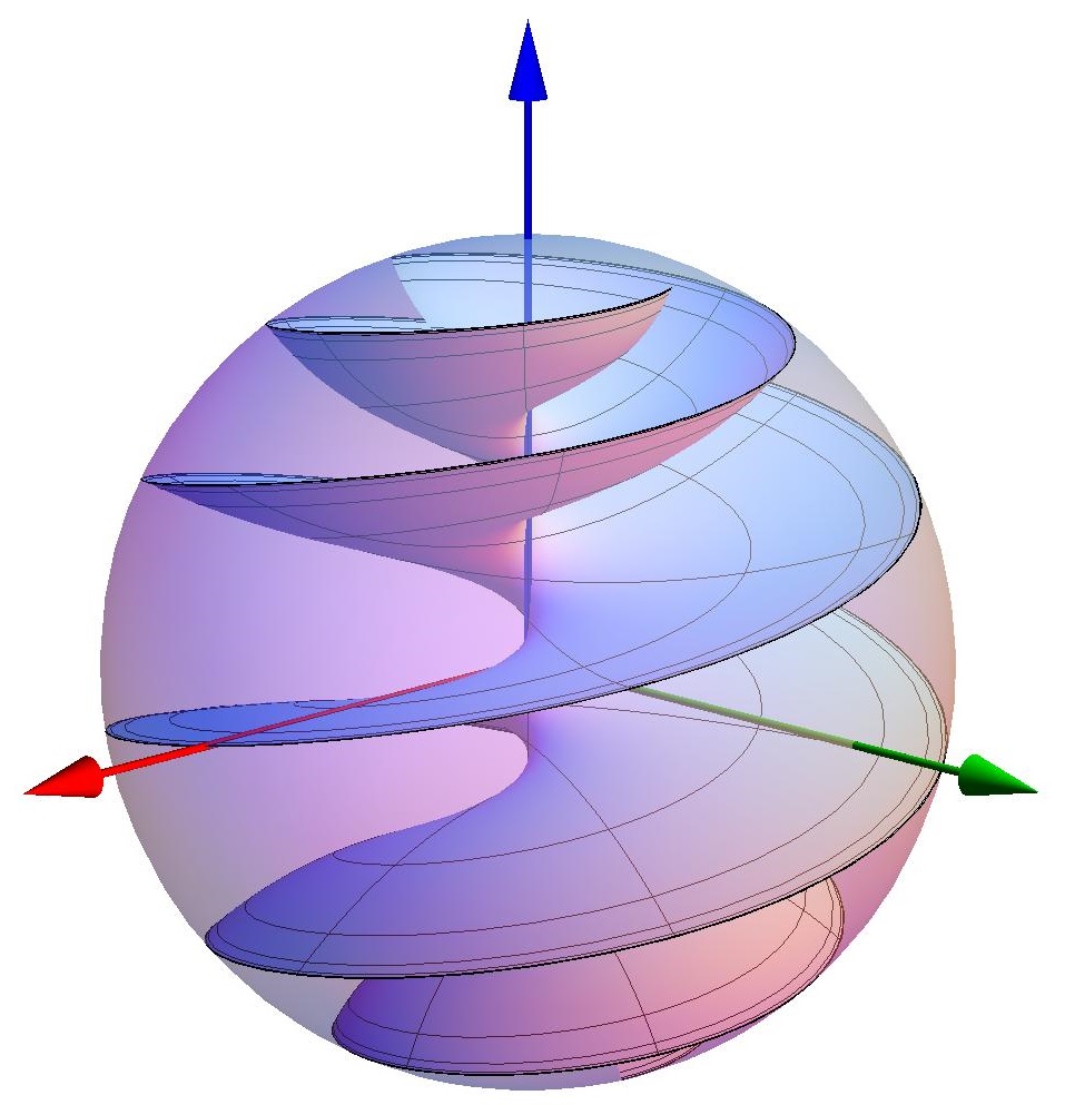
Figure 1. The helicoid $\mathcal{H}_{\bar{a}}$ with $\bar{a}=5$ in the Poincaré ball model of hyperbolic space. The curves perpendicular to the spirals are geodesics in $\mathbb{B}^{3}$.

2.4.3. Helicoids in $\mathbb{U}^{3}$

The helicoid $\mathcal{H}_{\bar{a}}$ in the upper half space model $\mathbb{U}^{3}$ of the hyperbolic $3$-space is given by (see Figure 2)

$$\mathcal{H}_{\bar{a}}=\{(z,t)\in\mathbb{U}^{3}\ |\ z=e^{v+\sqrt{-1}\,\bar{a}{}v}\tanh{}u\ \text{and}\ t=e^{v}\operatorname{sech}{}u\}\ ,$$ (2.16)

where $-\infty<u,v<\infty$, and the axis of $\mathcal{H}_{\bar{a}}$ is the $t$-axis.

From the equation (2.16), we can see that each helicoid $\mathcal{H}_{\bar{a}}$ is invariant under the one-parameter group $G_{\bar{a}}\subset\mathsf{PSL}_{2}(\mathbb{C})$ consisting of loxodromic transformations which fix the same $t$-axis , i.e.

$$G_{\bar{a}}=\left\{z\mapsto{}\exp\left(v+\sqrt{-1}\,\bar{a}{}v\right)z\ |\ -\infty<v<\infty\right\}\ .$$

When $v=0$, from (2.16) we get a semi unit circle in the $xt$-plane, whose center is the origin.

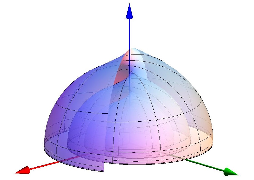
Figure 2. The helicoid $\mathcal{H}_{\bar{a}}$ with $\bar{a}=5$ in the upper half space model of hyperbolic space $\mathbb{H}^{3}$. The curves perpendicular to the spirals are geodesics in $\mathbb{H}^{3}$.

3. Existence and Uniqueness of Spherical Catenoids

In this section, we will prove a theorem of Gomes, which plays an important role in the paper [HW15] for constructing barrier surfaces.

3.1. Spherical catenoids in $\mathbb{B}^{3}$

In this subsection, we follow Hsiang (see [Hsi82, BdCH09]) to introduce the minimal spherical catenoids in $\mathbb{B}^{3}$. Let $X$ be a subset of $\mathbb{B}^{3}$, we define the asymptotic boundary of $X$ by

$$\partial_{\infty}X=\overline{X}\cap{}S_{\infty}^{2}\ ,$$ (3.1)

where $\overline{X}$ is the closure of $X$ in $\overline{\mathbb{B}}{}^{3}$.

Using the above notation, we have $\partial_{\infty}\mathbb{B}^{3}=S_{\infty}^{2}$. If $P$ is a geodesic plane in $\mathbb{B}^{3}$, then $P$ is perpendicular to $S_{\infty}^{2}$ and $C\stackrel{{\scriptstyle\text{def}}}{{=}}\partial_{\infty}P$ is an Euclidean circle on $S_{\infty}^{2}$. We also say that $P$ is asymptotic to $C$.

Suppose that $G\cong\mathsf{SO}(3)$ is a subgroup of $\mathsf{M\ddot{o}b}(\mathbb{B}^{3})$ that leaves a geodesic $\gamma\subset\mathbb{B}^{3}$ pointwise fixed. We call $G$ the spherical group of $\mathbb{B}^{3}$ and $\gamma$ the rotation axis of $G$. A surface in $\mathbb{B}^{3}$ which is invariant under $G$ is called a spherical surface or a surface of revolution. For two circles $C_{1}$ and $C_{2}$ in $\mathbb{B}^{3}$, if there is a geodesic $\gamma$, such that each of $C_{1}$ and $C_{2}$ is invariant under the group of rotations that fixes $\gamma$ pointwise, then $C_{1}$ and $C_{2}$ are said to be coaxial, and $\gamma$ is called the rotation axis of $C_{1}$ and $C_{2}$.

3.1.1. The warped product metric

Suppose that $G$ is the spherical group of $\mathbb{B}^{3}$ along the geodesic

$$\gamma_{0}=\{(u,0,0)\in\mathbb{B}^{3}\ |\ -1<u<1\}\ ,$$ (3.2)

then $\mathbb{B}^{3}/G\cong\mathbb{B}_{+}^{2}$, where

$$\mathbb{B}_{+}^{2}=\{(u,v)\in\mathbb{B}^{2}\ |\ v\geqslant{}0\}\ .$$ (3.3)

We shall equip the half space $\mathbb{B}_{+}^{2}$ with a warped product metric.

For any point $p=(u,v)\in\mathbb{B}_{+}^{2}$, there is a unique geodesic segment $\gamma^{\prime}$ passing through $p$ that is perpendicular to $\gamma_{0}$ at $q$. Let $x=\operatorname{dist}(O,q)$ and $y=\operatorname{dist}(p,q)=\operatorname{dist}(p,\gamma_{0})$ (see Figure 3), where $\operatorname{dist}(\cdot,\cdot)$ denotes the hyperbolic distance, then by [Bea95, Theorem 7.11.2], we have

$$\tanh{}x=\frac{2u}{1+(u^{2}+v^{2})}\quad\text{and}\quad\sinh{}y=\frac{2v}{1-(u^{2}+v^{2})}\ .$$ (3.4)

Equivalently, we also have

$$u=\frac{\sinh{}x\cosh{}y}{1+\cosh{}x\cosh{}y}\quad\text{and}\quad v=\frac{\sinh{}y}{1+\cosh{}x\cosh{}y}\ .$$ (3.5)

It’s well known that $\mathbb{B}_{+}^{2}$ can be equipped with the metric of warped product in terms of the parameters $x$ and $y$ as follows:

$$ds^{2}=\cosh^{2}y\cdot{}dx^{2}+dy^{2}\ ,$$ (3.6)

where $dx$ represents the hyperbolic metric on the geodesic $\gamma_{0}$ in (3.2). We call the horizontal geodesic $\{(u,0)\in\mathbb{B}_{+}^{2}\ |\ -1<u<1\}$ the $x$-axis and the vertical geodesic $\{(0,v)\in\mathbb{B}_{+}^{2}\ |\ 0\leqslant{}v<1\}$ the $y$-axis. The orientations of the $x$-axis and the $y$-axis are considered to be the same as that of the $u$-axis and the $v$-axis respectively. Thus we also consider that the $x$-axis and the $y$-axis are equivalent to the $u$-axis and the $v$-axis respectively.

Definition 3.1.

If $\mathcal{C}$ is a minimal surface of revolution in $\mathbb{B}^{3}$ with respect to the axis $\gamma_{0}$ in (3.2), then it is called a catenoid and the curve $\sigma=\mathcal{C}\cap\mathbb{B}_{+}^{2}$ is called the generating curve of $\mathcal{C}$ or a catenary.

Figure 3. For a point $p$ in $\mathbb{B}_{+}^{2}$ with the warped product metric, its coordinates $(x,y)$ are defined by $x=\operatorname{dist}(O,q)$ and $y=\operatorname{dist}(p,q)$.

3.1.2. Arc length parametrization of a catenary

Let $\sigma\subset\mathbb{B}_{+}^{2}$ be the generating curve of a minimal catnoid $\mathcal{C}$. Suppose that the parametric equations of $\sigma$ are given by: $x=x(s)$ and $y=y(s)$, where $s\in(-\infty,\infty)$ is an arc length parameter of $\sigma$. By the argument in [Hsi82, pp. 486–488], the curve $\sigma$ satisfies the following equations

$$\frac{2\pi\sinh{}y\cdot\cosh^{2}y}{\sqrt{\cosh^{2}{}y+(y^{\prime})^{2}}}=2\pi\sinh{}y\cdot\cosh{}y\cdot\sin\theta=k\ (\text{constant})\ ,$$ (3.7)

where $y^{\prime}=dy/dx$ and $\theta$ is the angle between the tangent vector of $\sigma$ and the vector $e_{y}=\partial/\partial{}y$ at the point $(x(s),y(s))$ (see Figure 4).

By the argument in [Gom87, pp.54–58]), up to isometry, we assume that the curve $\sigma$ is only symmetric about the $y$-axis (by assumption it’s the same as the $v$-axis) and intersects the $y$-axis orthogonally at $y_{0}=y(0)$, and so $y^{\prime}(0)=0$. Substitute these to (3.7), we get $k=2\pi\sinh(y_{0})\cosh(y_{0})$, and then we have the following equation

$$\sin\theta=\frac{\sinh(y_{0})\cosh(y_{0})}{\sinh(y)\cosh(y)}=\frac{\sinh(2y_{0})}{\sinh(2y)}\ .$$ (3.8)

Now we solve for $dx/dy$ in terms of $y$ in (3.7) and integrate $dx/dy$ from $y_{0}$ to $y$ for any $y\geqslant{}y_{0}$, then we have the following equality

$$x(y)=\int_{y_{0}}^{y}\frac{\sinh(2y_{0})}{\cosh{}y}\frac{dy}{\sqrt{\sinh^{2}(2y)-\sinh^{2}(2y_{0})}}\ .$$ (3.9)

Let $y\to\infty$ in (3.9), we get (see Figure 5)

$$x(\infty)=\int_{y_{0}}^{\infty}\frac{\sinh(2y_{0})}{\cosh{}y}\frac{dy}{\sqrt{\sinh^{2}(2y)-\sinh^{2}(2y_{0})}}\ .$$ (3.10)

We can see that the hyperbolic distance between two totally geodesic planes bounded by the boundary of the catenoid $\mathcal{C}$, whose generating curve is $\sigma$, is equal to the double of $x(\infty)$. We will see that this distance can not be too large, actually it’s around $1$ (see Theorem 3.4).

Figure 4. $\theta$ is the angle between the parametrized curve $\sigma$ and the geodesic $\gamma^{\prime}$ at the point $(x(s),y(s))\in\sigma\cap\gamma^{\prime}$, where $\gamma^{\prime}$ is perpendicular to the $u$-axis.

Replacing the initial data $y_{0}$ by a parameter $a\in(0,\infty)$ in (3.9), and let $\sigma_{a}\subset\mathbb{B}_{+}^{2}$ be the catenary which is symmetric about the $y$-axis and whose initial data is $a$ (actually the hyperbolic distance between $\sigma_{a}$ and the origin of $\mathbb{B}_{+}^{2}$ is equal to $a$).

In order to get the parametric equation of the catenary $\sigma_{a}$ with arc length, we define a function of the variable $a$ by rewriting (3.9):

$$\rho(a,t)=\int_{a}^{t}\frac{\sinh(2a)}{\cosh\tau}\frac{d\tau}{\sqrt{\sinh^{2}(2\tau)-\sinh^{2}(2a)}}\ ,\quad{}t\geqslant{}a\ .$$ (3.9^′)

Recall that the semi disk $\mathbb{B}_{+}^{2}$ is equipped with the metric (3.6), it’s easy to get the arc length of the catenary $\sigma_{a}$:

$$s(a,t)=\int_{a}^{t}\frac{\sinh(2\tau)}{\sqrt{\cosh^{2}(2\tau)-\cosh^{2}(2a)}}\,d\tau=\frac{1}{2}\,\cosh^{-1}\left(\frac{\cosh(2t)}{\cosh(2a)}\right)\ ,$$ (3.11)

where $t\geqslant{}a$. For any $s\in(-\infty,\infty)$, let

$$x(a,s) =\sqrt{2}\,\sinh(2a)\int_{0}^{s}\frac{\sqrt{\cosh(2a)\cosh(2t)-1}}{\cosh^{2}(2a)\cosh^{2}(2t)-1}\,dt\ ,$$ (3.12)

$$y(a,s) =a+\int_{0}^{s}\frac{\cosh(2a)\sinh(2t)}{\sqrt{\cosh^{2}(2a)\cosh^{2}(2t)-1}}\,dt$$ (3.13)

$$=\frac{1}{2}\,\cosh^{-1}(\cosh^{2}(2a)\cosh^{2}(2s))\ .$$ (3.14)

It’s easy to verify that

$$x(a,s)=\rho(a,y(a,s))$$ (3.15)

for $s\geqslant{}0$ and that the map

$$s\mapsto(x(a,s),y(a,s))$$ (3.16)

is arc-length parametrization of the catenary $\sigma_{a}$ for $s\in(-\infty,\infty)$, where $\rho(\cdot,\cdot)$ is given by (3.9^′) (see [BSE10, Proposition 4.2]).

Figure 5. The distance $x(\infty)$ defined in (3.10) is equal to $\operatorname{dist}(O,q)$, where the point $q$ is the intersection of the $u$-axis and the unique geodesic which is perpendicular to both the $u$-axis at $q$ and $\partial_{\infty}\mathbb{B}_{+}^{2}$ at $p_{\infty}$ (here $p_{\infty}$ is one of the asymptotic boundary points of $\sigma$ given by (3.16)). In this figure, $y_{0}=0.4$, and so $x(\infty)\approx{}0.49268$.

3.1.3. Parametrization of a catenoid

Definition 3.2.

The surface of revolution along the axis $\gamma_{0}$ in (3.2) generated by the catenary $\sigma_{a}$ (3.16) is called a catenoid, and is denoted by $\mathcal{C}_{a}$ for $0<a<\infty$.

Next we shall find the parametric equation of the catenoid $\mathcal{C}_{a}$. Recall that the generating curve $\sigma_{a}$ of the catenoid $\mathcal{C}_{a}$ is parametrized by arc length: $x=x(a,s)$ and $y=y(a,s)$ given by (3.12), (3.13) and (3.14). Just as in (3.5), we define

$$u(a,s)=\frac{\sinh{}x\cosh{}y}{1+\cosh{}x\cosh{}y}\quad\text{and}\quad v(a,s)=\frac{\sinh{}y}{1+\cosh{}x\cosh{}y}\ .$$

The parametric equation of the catenoid $\mathcal{C}_{a}$ in $\mathbb{B}^{3}$ is given by

$$Y(a,s,\theta)=\begin{pmatrix}u\\ v\omega_{\theta}\end{pmatrix}\ ,\quad s\in\mathbb{R}\ \text{and}\ \theta\in[0,2\pi]\ ,$$ (3.17)

where $\omega_{\theta}=\begin{pmatrix}\cos\theta\\ \sin\theta\end{pmatrix}$. Direct computation shows that the unit normal vector of the catenoid $\mathcal{C}_{a}$ at $Y(a,s,\theta)$ is

$$N(a,s,\theta)=\begin{pmatrix}v_{s}\\ -u_{s}\omega_{\theta}\end{pmatrix}\ ,\quad s\in\mathbb{R}\ \text{and}\ \theta\in[0,2\pi]\ ,$$ (3.18)

where $u_{s}$ and $v_{s}$ are the partial derivatives of $u$ and $v$ on $s$ respectively.

Remark 3.3.

The spherical catenoid $\mathscr{C}_{1}(\tilde{a})$ in the hyperboloid model $\mathbf{H}^{3}$ is isometric to the spherical catenoid $\mathcal{C}_{a}$ in the Poincaré ball model $\mathbb{B}^{3}$ if and only if $2\tilde{a}=\cosh(2a)$ (see Lemma 6.3).

3.2. The theorem of Gomes

Obviously the asymptotic boundary of any spherical catenoid $\mathcal{C}_{a}$ is the union of two circles (see also [Gom87, Proposition 3.1]). It’s important for us to determine whether there exists a minimal spherical catenoid asymptotic to any given pair of disjoint circles on $S_{\infty}^{2}$, since in [HW15] we construct quasi-Fuchsian $3$-manifolds which contain arbitrarily many incompressible minimal surface by using the (least area) minimal spherical catenoids as the barrier surfaces.

If $C_{1}$ and $C_{2}$ are two disjoint circles on $S_{\infty}^{2}$, then they are always coaxial. In fact, let $P_{1}$ and $P_{2}$ be the geodesic planes asymptotic to $C_{1}$ and $C_{2}$ respectively, there always exists a unique geodesic $\gamma$ such that $\gamma$ is perpendicular to both $P_{1}$ and $P_{2}$. Therefore $C_{1}$ and $C_{2}$ are coaxial with respect to $\gamma$. We may define the distance between $C_{1}$ and $C_{2}$ by

$$d_{L}(C_{1},C_{2})=\operatorname{dist}(P_{1},P_{2})\ .$$ (3.19)

In order to prove Theorem 3.4, we need define a function $\varrho(a)$ of the parameter $a$. Let $t$ approach infinity in (3.9^′), we define the function

$$\varrho(a)=\rho(a,\infty)=\int_{a}^{\infty}\frac{\sinh(2a)}{\cosh{}t}\frac{dt}{\sqrt{\sinh^{2}(2t)-\sinh^{2}(2a)}}\ .$$ (3.20)

Using the substitution $t\mapsto{}t+a$, the above function (3.20) can be written as

$$\varrho(a)=\int_{0}^{\infty}\frac{\sinh(2a)}{\cosh(a+t)}\frac{dt}{\sqrt{\sinh^{2}(2a+2t)-\sinh^{2}(2a)}}\ .$$ (3.20^′)

Theorem 3.4 (Gomes).

There exists a constant $a_{c}\approx{}0.49577$ such that for two disjoint circles $C_{1},C_{2}\subset{}S_{\infty}^{2}$, if

$$d_{L}(C_{1},C_{2})\leqslant{}2\varrho(a_{c})\approx{}1.00229\ ,$$

then there exist a spherical minimal catenoid $\mathcal{C}$ which is asymptotic to $C_{1}\cup{}C_{2}$, where $\varrho(a)$ is the function defined by (3.20).

Remark 3.5.

In [dOS98, p. 402], de Oliveria and Soret show that for any two congruent circles (in $\partial_{\infty}\mathbb{U}^{3}=\mathbb{R}^{2}\times\{0\}$) of Euclidean diameter $d$ and disjoint from each other by the Euclidean distance $D$, there exists two catenoids bounding the two circles if and only if $D/d\leqslant\delta$ for some $\delta>0$. Direct computation shows that $\delta=\cosh(\varrho(a_{c}))-1\approx{}0.12763$, where $\varrho(a)$ is the function defined by (3.20) and $a_{c}$ is the unique critical number of the function $\varrho(a)$.

Figure 6. The graph of the function $\varrho(a)$ defined by (3.20) for $a\in[0,3]$. It seems that $\varrho(a)$ only has a unique critical number.

Proof of Theorem 3.4.

Let $\varrho(a)$ be the function defined by (3.20) or (3.20^′). We claim that $\varrho(0)=0$, and as $a$ increases $\varrho(a)$ increases monotonically, reaches a maximum, then decreases asymptotically to zero as $a$ goes to infinity (see also [Gom87, Proposition 3.2] and Figure 6).

It’s easy to show $\varrho(a)\to{}0$ as $a\to\infty$. In fact, we have

$$\varrho(a) =\int_{0}^{\infty}\frac{\sinh(2a)}{\cosh(a+t)}\frac{dt}{\sqrt{\sinh^{2}(2a+2t)-\sinh^{2}(2a)}}$$

$$=\int_{0}^{\infty}\frac{1}{\cosh(t+a)}\frac{dt}{\sqrt{\left(\dfrac{\sinh(2a+2t)}{\sinh(2a)}\right)^{2}-1}}$$

$$<\int_{0}^{\infty}\frac{1}{\cosh{}a}\frac{dt}{\sqrt{(\sinh(2t)+\cosh(2t))^{2}-1}}\ .$$

Since $\sinh(2t)+\cosh(2t)=e^{2t}$, we have

$$\varrho(a) <\frac{1}{\cosh{}a}\int_{0}^{\infty}\frac{dt}{\sqrt{e^{4t}-1}}=\frac{1}{\cosh{}a}\int_{0}^{\infty}\frac{e^{-2t}}{\sqrt{1-e^{-4t}}}\,dt$$ (3.21)

$$=\frac{1}{\cosh{}a}\cdot\frac{\pi}{4}\longrightarrow{}0\quad\text{as}\ a\to\infty\ .$$

Besides, since $\displaystyle\lim_{a\to{}0^{+}}\varrho(a)=0$, $\varrho(a)>0$ for $a\in(0,\infty)$ and $\varrho(a)\to{}0$ as $a\to\infty$, it must have at least one maximum value in $(0,\infty)$.

By the argument in the proof of Theorem 1.2 in $\S$4, we know that $\varrho^{\prime}(a)$ has a unique zero $a_{c}$ such that $\varrho^{\prime}(a)>0$ if $0<a<a_{c}$ and $\varrho^{\prime}(a)<0$ if $a>a_{c}$, hence the proof of the claim is complete. According to the numerical computation: the function $\varrho(a)$ achieves its (unique) maximum value $\approx{}0.501143$ when $a=a_{c}\approx{}0.49577$, and so $2\varrho(a_{c})\approx{}1.00229$. ∎

Theorem 3.4 shows the existence of spherical minimal catenoids. On the other hand, we also have the uniqueness of catenoids in the sense of following theorem proved by Levitt and Rosenberg (see [LR85, Theorem 3.2] and [dCGT86, Theorem 3]). Recall that a complete minimal surface $\Sigma$ of $\mathbb{H}^{3}$ is regular at infinity if $\partial_{\infty}\Sigma$ is a $C^{2}$-submanifold of $S^{2}_{\infty}$ and $\overline{\Sigma}=\Sigma\cup\partial_{\infty}\Sigma$ is a $C^{2}$-surface (with boundary) of $\overline{\mathbb{H}^{3}}$.

Theorem 3.6 (Levitt and Rosenberg).

Let $C_{1}$ and $C_{2}$ be two disjoint round circles on $S_{\infty}^{2}$ and let $\mathcal{C}$ be a connected minimal surface immersed in $\mathbb{H}^{3}$ with $\partial_{\infty}\mathcal{C}=C_{1}\cup{}C_{2}$ and $\mathcal{C}$ regular at infinity. Then $\mathcal{C}$ is a spherical catenoid.

4. Stability of Spherical Catenoids

In this section we will prove Theorem 1.2. Let $\Sigma$ be a complete minimal surface immersed in a complete Riemannian $3$-manifold $M^{3}$, and let $\Omega$ be any subdomain of $\Sigma$. Recall that a Jacobi field on $\Omega\subset\Sigma$ is a $C^{\infty}$ function $\phi$ such that $\mathcal{L}\phi=0$ on $\Omega$.

According to Theorem 2.3, in order to show that a complete minimal surface $\Sigma\subset{}M^{3}$ is stable, we just need to find a positive Jacobi field on $\Sigma$. On the other hand, if a Jacobi field on $\Sigma$ changes its sign between the interior and the exterior of a compact subdomain $\Omega$ of $\Sigma$ and vanishes on $\partial\Omega$, we can conclude that $\Omega$ is a maximally weakly stable minimal surface, which also implies that $\Sigma$ is unstable.

The geometry of the ambient space provides useful Jacobi fields. More precisely, we have the following classical results.

Theorem 4.1 ([Xin03, pp. 149–150]).

Let $\Sigma$ be a complete minimal surface immersed in complete Riemannian $3$-manifold $M^{3}$ and let $V$ be a Killing field on $M^{3}$. The function $\zeta=\langle V\,,N\rangle$, given by the inner product in $M^{3}$ of the Killing field $V$ with the unit normal $N$ to the immersion, is a Jacobi field on $\Sigma$.

Theorem 4.2 ([BdC80, Theorem 2.7]).

Let $X(a,\cdot):\Sigma\to{}M^{3}$ be a $1$-parameter family of minimal immersions. Then, for each fixed $a_{0}$, the function

$$\xi=\left\langle\frac{\partial{X}}{\partial{a}}(a_{0},\cdot)\,,\,N\right\rangle$$

is a Jacobi field on $X(a_{0},\Sigma)$, where $\langle\cdot\,,\cdot\rangle$ is the inner product in $M^{3}$ and $N$ is the unit normal vector field on the minimal surface $X(a_{0},\Sigma)$.

4.1. Jacobi fields on spherical catenoids

Next we will follow Bérard and Sa Earp [BSE10] to introduce the vertical Jacobi fields and the variation Jacobi fields on the minimal spherical catenoids $\{\mathcal{C}_{a}\}_{a>0}$ in $\mathbb{B}^{3}$, which will be used to prove Theorem 1.2.

Definition 4.3.

Let $V$ be the Killing vector field associated with the hyperbolic translations along the geodesic $t\mapsto(\tanh(t/2),0,0)\in\mathbb{B}^{3}$. The vertical Jacobi field on the catenoid $\mathcal{C}_{a}$ is the function

$$\zeta(a,s)=\langle V(a,s,\theta)\,,N(a,s,\theta)\rangle\ ,$$ (4.1)

where $V(a,s,\theta)$ is the restriction of the Killing vector field $V$ to the minimal catenoid $\mathcal{C}_{a}$ defined by (3.17).

The variation Jacobi field on the catenoid $\mathcal{C}_{a}$ is

$$\xi(a,s)=-\langle Y_{a}(a,s,\theta)\,,N(a,s,\theta)\rangle\ ,$$ (4.2)

where $Y_{a}=\frac{\partial{Y}}{\partial{a}}$.

In order to find the detail expressions of the vertical and the variation Jacobi fields on the catenoids, we need some notations (see [BSE10, $\S$4.2]). Let

$$f(a,s)=\frac{\sinh^{2}(2a)\cosh(2s)}{\cosh^{2}(2a)\cosh^{2}(2s)-1}\ ,$$ (4.3)

and let

$$I(a,t)=\frac{n(\cosh(2a),\cosh(2t))}{d(\cosh(2a),\cosh(2t))}$$ (4.4)

where

• $n(A,T)=A(3-A^{2})T^{2}+(A^{2}-1)T-2A$, and

• $d(A,T)=(AT+1)^{2}(AT-1)^{3/2}$.

For the functions $x(a,s)$ and $y(a,s)$ given by (3.12) and (3.13), the notations $x_{a}$, $x_{s}$, $y_{a}$ and $y_{s}$ denote the partial derivatives of $x(a,s)$ and $y(a,s)$ on $a$ and $s$ respectively.

Proposition 4.4 ([BSE10, $\S$4.2.1]).

The vertical Jacobi field $\zeta(a,s)$ is given by

$$\zeta(a,s)=\sqrt{2}\,\cosh(y(a,s))y_{s}(a,s)=\frac{\cosh(2a)\sinh(2s)}{\sqrt{\cosh(2a)\cosh(2s)-1}}\ .$$ (4.5)

The variation Jacobi field $\xi(a,s)$ is given by

$$\xi(a,s) =-\cosh(y(a,s))(x_{a}(a,s)y_{s}(a,s)-x_{s}(a,s)y_{a}(a,s))$$ (4.6)

$$=f(a,s)-\zeta(a,s)\int_{0}^{s}I(a,t)dt\ ,$$ (4.7)

where $f(a,s)$ and $I(a,t)$ are given by (4.3) and (4.4) respectively.

Since $x(a,\infty)$ is well defined for any $a>0$, we may set

$$E(a)=\frac{d{}}{d{a}}\,x(a,\infty)=\sqrt{2}\int_{0}^{\infty}I(a,t)dt\ .$$ (4.8)

Equivalently we have the following identity (see [BSE10, p. 3665]):

$$E(a)=\frac{\varrho^{\prime}(a)}{\sqrt{2}}\ ,$$ (4.9)

where $\varrho^{\prime}(a)$ is defined by (4.13), which is derivative of the function $\varrho(a)$ given by (3.20).

For any (connected) interval $\mathbf{I}\subset\mathbb{R}$, we define

$$\mathcal{C}(a,\mathbf{I})=\{Y(a,s,\theta)\in\mathbb{B}^{3}\ |\ s\in{}\mathbf{I}\ \text{and}\ \theta\in[0,2\pi]\}\ ,$$ (4.10)

where $Y(a,s,\theta)$ is given by (3.17). Obviously $\mathcal{C}(a,\mathbf{I})\subset\mathcal{C}_{a}$.

Lemma 4.5 ([BSE10, Lemma 4.5]).

For any constant $a>0$, the half catenoids $\mathcal{C}(a,(-\infty,0])$ and $\mathcal{C}(a,[0,\infty))$ are both stable.

Any Jacobi field $\eta(a,s)$ depending only on the radial variable s on $\mathcal{C}_{a}$ can change its sign at most once on either $(-\infty,0]$ or $[0,\infty)$.

Proof.

The first part follows from the fact that $\zeta(a,s)$ doesn’t change its sign on either $\mathcal{C}(a,(-\infty,0])$ or $\mathcal{C}(a,[0,\infty))$ and $\mathcal{L}{}\zeta=0$.

Assume that some Jacobi field $\eta(a,s)$ on $\mathcal{C}_{a}$ changes its sign more than once on $[0,\infty)$, then $\eta(a,s)$ has at least two zeros on $[0,\infty)$, say $0<{}z_{1}<z_{2}<\cdots$. Let $\mathbf{I}=[z_{1},z_{2}]$ and let $\phi(a,s)$ be the restriction of $\eta(a,s)$ to $\mathcal{C}(a,\mathbf{I})$, then we have $\phi\in{}C_{0}^{\infty}(\mathcal{C}(a,\mathbf{I}))$ and $\mathcal{L}{}\phi=0$, which imply that $\lambda_{1}(\mathcal{C}(a,\mathbf{I}))\leqslant{}0$. This is a contradiction, since $\mathcal{C}(a,\mathbf{I})$ is a compact connected subdomain of $\mathcal{C}(a,[0,\infty))$, which must be stable. ∎

The following theorem, whose proof can be found in [BSE10, p. 3663], is crucial to the proof of Theorem 1.2. Because of (4.9), (4.13) and Lemma 7.1, we always have $\cosh^{2}(2a)<3$ if $E(a)=0$, hence it is not necessary to consider the case when $\cosh^{2}(2a)<3$ in the the proof of [BSE10, Theorem 4.7 (1)].

Theorem 4.6 ([BSE10, Theorem 4.7 (1)]).

Let $\sigma_{a}$ be the catenary given by (3.9) and let $\mathcal{C}_{a}$ be the minimal surface of revolution along the $u$-axis whose generating curve is the catenary $\sigma_{a}$.

1. If $E(a)\leqslant{}0$, then $\mathcal{C}_{a}$ is stable.

2. If $E(a)>0$, then $\mathcal{C}_{a}$ is unstable and has index $1$.

Proof.

(1) As state in Lemma 4.5, the function $\xi(a,s)$ can change its sign at most once on $(0,\infty)$ and $(-\infty,0)$ respectively. Observe that the function $\xi(a,s)$ is even and that $\xi(a,0)=1$. To determine whether $\xi$ has a zero, it suffices to look at its behaviour at infinity.

If $E(a)<0$, then $\int_{0}^{\infty}I(a,t)dt<0$, which implies that $\xi(a,s)\to\infty$ as $s\to\pm\infty$, therefore $\xi(a,s)>0$ for all $s\in(-\infty,\infty)$.

If $E(a)=0$, we have the following equation

$$\xi(a,s)=f(a,s)+\zeta(a,s)\int_{s}^{\infty}I(a,t)dt\ .$$ (4.11)

By (4.9), (4.13) and Lemma 7.1, we can see that if $E(a)=0$, then

$$\cosh^{2}(2a)\leqslant\cosh^{2}(2A_{3})=\left(\frac{1+\sqrt{5}}{2}\right)^{2}<3\ ,$$

and so $I(a,t)>0$ if $t$ is large enough. If $s$ is sufficiently large, then $\xi(a,s)>0$ according to (4.11), thus $\xi(a,s)>0$ for all $s\in(-\infty,\infty)$. Therefore $\mathcal{C}_{a}$ is stable if $E(a)\leqslant{}0$.

(2) Recall that the variation Jacobi field $\xi(a,s)$ can change its sign at most once on either $(0,\infty)$ or $(-\infty,0)$ by Lemma 4.5. Now suppose that $E(a)>0$, since $\xi(a,0)=1$ and $\xi(a,s)\to-\infty$ as $s\to\pm\infty$, we know that $\xi(a,s)$ has exactly two symmetric zeros in $(-\infty,\infty)$, which are denoted by $\pm{}z(a)$. Let $\mathcal{C}(z(a))$ be the subdomain of $\mathcal{C}_{a}$ defined by

$$\mathcal{C}(z(a))=\mathcal{C}(a,[-z(a),z(a)])\ .$$ (4.12)

Let $\phi(a,s)$ be restriction of $\xi(a,s)$ to $\mathcal{C}(z(a))$, then $\phi\in{}C_{0}^{\infty}(\mathcal{C}(z(a)))$ and $\mathcal{L}{}\phi=0$. This implies that $\lambda_{1}(\mathcal{C}(z(a)))\leqslant{}0$, which can imply that any compact connected subdomain of $\mathcal{C}_{a}$ containing $\mathcal{C}(z(a))$ must be unstable by Lemma 2.1.

Therefore $\mathcal{C}_{a}$ has index at least one. By [Seo11, Theorem 4.3] or [Tuz93, $\S$3.3], $\mathcal{C}_{a}$ has index one. ∎

4.2. Proof of Theorem 1.2

Now we are able to prove Theorem 1.2.

Figure 7. The derivative of the function $\varrho(a)$ for $a\in(0,3]$. From the figure we can see that $\varrho^{\prime}(a)$ has a unique zero, which is very close to $0.5$.

Theorem 1.2.

There exists a constant $a_{c}\approx{}0.49577$ such that the following statements are true:

1. $\mathcal{C}_{a}$ is an unstable minimal surface with Morse index one if $0<a<a_{c}$;

2. $\mathcal{C}_{a}$ is a globally stable minimal surface if $a\geqslant{}a_{c}$.

Proof.

Recall that we have $E(a)=\varrho^{\prime}(a)/\sqrt{2}$ by (4.9). We claim that $\varrho^{\prime}(a)$ satisfies the following conditions (see Figure 7):

• $\varrho^{\prime}(a)\to\infty$ as $a\to{}0^{+}$ and $\varrho^{\prime}(a)<0$ on $[A_{3},\infty)$, and

• $\varrho^{\prime}(a)$ is decreasing on $(0,A_{4})$,

where $A_{3}<A_{4}$ are constants defined in (7.1) and (7.3). These conditions can imply that $\varrho^{\prime}$ has a unique zero $a_{c}\in(0,\infty)$ such that $\varrho^{\prime}(a)>0$ if $0<a<a_{c}$ and $\varrho^{\prime}(a)<0$ if $a>a_{c}$, hence together with Theorem 4.6, the theorem follows.

Next let’s prove the above claim. It’s easy to verify that

$$\varrho^{\prime}(a)=\int_{0}^{\infty}\frac{\sinh(a+t)(5\cosh^{2}(a+t)-\cosh^{2}(3a+t))}{\cosh^{2}(a+t)\sqrt{\sinh(2t)\sinh^{3}(4a+2t)}}\,dt\ .$$ (4.13)

By Lemma 7.1, $\varrho^{\prime}(a)<0$ on $(A_{3},\infty)$. Now let

$$h(a,t)=\frac{\sinh(a+t)(5\cosh^{2}(a+t)-\cosh^{2}(3a+t))}{\cosh^{2}(a+t)\sqrt{\sinh(2t)\sinh^{3}(4a+2t)}}\ .$$ (4.14)

Then for any fixed constant $a>0$, we have the estimates

$$h(a,t)\sim{}C_{1}(a)\left(\sqrt{\sinh{}t}+\frac{\cosh{}t}{\sqrt{\sinh{}t}}\right)\ ,\quad\text{as}\ t\to{}0\ ,$$ (4.15)

and

$$h(a,t)\sim\frac{C_{2}(a)}{\cosh{}t\cosh(2a+t)\sinh(4a+2t)}\ ,\quad\text{as}\ t\to\infty\ .$$ (4.16)

Hence $\varrho^{\prime}(a)$ is well defined for $a>0$, and then

$$\lim_{a\to{}0^{+}}\varrho^{\prime}(a) =\int_{0}^{\infty}\frac{1}{\sinh{}t\cosh^{2}t}\,dt$$

$$=\left[\log\left(\frac{\cosh{}t-1}{\cosh{}t+1}\right)+\frac{1}{\cosh{}t}\right]_{t=0}^{t=\infty}=\infty\ .$$

Next, we have

$$\varrho^{\prime\prime}(a)=\int_{0}^{\infty}\frac{\psi(a,t)}{16\cosh^{3}(a+t)\sqrt{\sinh(2t)\sinh^{5}(4a+2t)}}\,dt\ ,$$ (4.17)

where $\psi(a,t)$ is the function defined by (7.2). By the result in Lemma 7.2, $\varrho^{\prime\prime}(a)<0$ for $a\in(0,A_{4})$, thus $\varrho^{\prime}(a)$ is decreasing on $(0,A_{4})$. ∎

5. Least Area Spherical Catenoids

In this section, we will prove Theorem 1.4. The following estimate is crucial to the proof of Theorem 1.4.

Lemma 5.1.

For all real numbers $a>0$, consider the functions

$$f(a)=\int_{a}^{\infty}\sinh{}t\cdot\left(\frac{\sinh(2t)}{\sqrt{\sinh^{2}(2t)-\sinh^{2}(2a)}}-1\right)dt\ ,$$ (5.1)

and $g(a)=\cosh{}a-1$, then we have the following results:

1. $f(a)$ is well defined for each fixed $a\in(0,\infty)$.

2. $f(a)<g(a)$ for sufficiently large $a$.

Proof.

(1) Using the substitution $t\to{}t+a$, we have

$$f(a)=\int_{0}^{\infty}\sinh(a+t)\left(\frac{\sinh(2a+2t)}{\sqrt{\sinh^{2}(2a+2t)-\sinh^{2}(2a)}}-1\right)dt\ .$$

We will prove that $f(a)<K\cosh{}a$, where

$$K=\int_{0}^{1}\frac{1}{x^{2}}\left(\frac{1}{\sqrt{1-x^{4}}}-1\right)dx$$ (5.2)

is a constant between $0$ and $1$.

Let $\displaystyle\Phi(a,t)=\frac{\sinh(2a+2t)}{\sqrt{\sinh^{2}(2a+2t)-\sinh^{2}(2a)}}$, then for any fixed $t\in[0,\infty)$, it’s easy to verify that $\Phi(a,t)$ is increasing on $[0,\infty)$ with respect to $a$. So we have the estimate

$$\Phi(a,t) \leqslant\lim_{a\to\infty}\frac{\sinh(2a+2t)}{\sqrt{\sinh^{2}(2a+2t)-\sinh^{2}(2a)}}$$

$$=\frac{\sinh(2t)+\cosh(2t)}{\sqrt{(\sinh(2t)+\cosh(2t))^{2}-1}}$$

$$=\frac{e^{2t}}{\sqrt{e^{4t}-1}}=\frac{1}{\sqrt{1-e^{-4t}}}\ .$$

Besides, $\sinh(a+t)<(\sinh{}t+\cosh{}t)\cosh{}a=e^{t}\cosh{}a$, therefore we have the following estimate

$$f(a) <\cosh{}a\int_{0}^{\infty}e^{t}\left(\frac{e^{2t}}{\sqrt{e^{4t}-1}}-1\right)dt$$

$$=\cosh{}a\int_{0}^{\infty}e^{t}\left(\frac{1}{\sqrt{1-e^{-4t}}}-1\right)dt$$

$$=\cosh{}a\int_{0}^{1}\frac{1}{x^{2}}\left(\frac{1}{\sqrt{1-x^{4}}}-1\right)dx\quad(t\mapsto{}x=e^{-t})$$

Since $x^{2}+1\geqslant{}1$, we have

$$K =\int_{0}^{1}\frac{1}{x^{2}}\left(\frac{1}{\sqrt{1-x^{4}}}-1\right)dx$$

$$<\int_{0}^{1}\frac{1}{x^{2}}\left(\frac{1}{\sqrt{1-x^{2}}}-1\right)dx=1\ ,$$

where we use the substitution $x\to{}\sin{}x$ to evaluate the above integral.

(2) We have proved that $f(a)<K\cosh{}a$ for any $a\in[0,\infty)$. Let

$$a_{l}=\cosh^{-1}\left(\frac{1}{1-K}\right)\ ,$$ (5.3)

then $f(a)<g(a)$ if $a\geqslant{}a_{l}$. ∎

Remark 5.2.

The function $f(a)$ in (5.1) has its geometric meaning: $2\pi{}f(a)$ is the difference of the infinite area of one half of the catenoid $\mathcal{C}_{a}$ and that of the annulus

$$\mathcal{A}=\{(0,v,w)\in\mathbb{B}^{3}\ |\ \tanh(a/2)\leqslant\sqrt{v^{2}+w^{2}}<1\}\ .$$

Remark 5.3.

The first definite integral in (5.2) is an elliptic integral. By the numerical computation, $K\approx{}0.40093$, and hence $a_{l}\approx{}1.10055$.

We need the coarea formula that will be used in the proof of Theorem 1.4. The proof of (5.4) in Lemma 5.4 can be found in [Wan12].

Lemma 5.4 (Calegari and Gabai [CG06, $\S$1]).

Suppose $\Sigma$ is a surface in the hyperbolic $3$-space $\mathbb{B}^{3}$. Let $\gamma\subset\mathbb{B}^{3}$ be a geodesic, for any point $q\in\Sigma$, define $\theta(q)$ to be the angle between the tangent space to $\Sigma$ at $q$, and the radial geodesic that is through $q$ (emanating from $\gamma$) and is perpendicular to $\gamma$. Then

$$\operatorname{Area}(\Sigma\cap\mathscr{N}_{s}(\gamma))=\int_{0}^{s}\int_{\Sigma\cap\partial\mathscr{N}_{t}(\gamma)}\frac{1}{\cos\theta}\,dldt\ ,$$ (5.4)

where $\mathscr{N}_{s}(\gamma)$ is the hyperbolic $s$-neighborhood of the geodesic $\gamma$.

Figure 8. The curve $\wideparen{p_{-}p_{+}}=\Sigma\cap\mathbb{B}_{+}^{2}$ is the portion of the catenary $\sigma_{a}$ with $a=1.2$. The curves $\wideparen{p_{+}q_{+}}=P_{+}\cap\mathbb{B}_{+}^{2}$ and $\wideparen{p_{-}q_{-}}=P_{-}\cap\mathbb{B}_{+}^{2}$. In this figure, $y_{1}=2.4$ and $x_{1}\approx{}0.330439$. By numerical computation: $\operatorname{Area}(\Sigma)=54.6636$ and $\operatorname{Area}(P_{+}\cup{}P_{-})=57.2643$.

Now we are able to prove Theorem 1.4.

Theorem 1.4.

There exists a constant $a_{l}\approx{}1.10055$ defined by (5.3) such that for any $a\geqslant{}a_{l}$ the catenoid $\mathcal{C}_{a}$ is a least area minimal surface in the sense of Meeks and Yau.

Proof.

First of all, suppose that $a\geqslant{}a_{l}$ is an arbitrary constant. Suppose that $\partial_{\infty}\mathcal{C}_{a}=C_{1}\cup{}C_{2}$, and let $P_{i}$ be the geodesic plane asymptotic to $C_{i}$ ($i=1,2$). Let $\sigma_{a}=\mathcal{C}_{a}\cap\mathbb{B}_{+}^{2}$ be the generating curve of the catenoid $\mathcal{C}_{a}$.

For $x\in(-\varrho(a),\varrho(a))$, where $\varrho(a)$ is defined by (3.20), let $P(x)$ be the geodesic plane perpendicular to the $u$-axis such that $\operatorname{dist}(O,P(x))=|x|$. Now let

$$\Sigma=\bigcup_{|x|\leqslant{}x_{1}}\left(\mathcal{C}_{a}\cap{}P(x)\right)\ ,$$ (5.5)

for some $0<x_{1}<\varrho(a)$. Let $\partial\Sigma=C_{+}\cup{}C_{-}$. Note that $C_{+}$ and $C_{-}$ are coaxial with respect to the $u$-axis.

Claim 1.

$\operatorname{Area}(\Sigma)<\operatorname{Area}(P_{+})+\operatorname{Area}(P_{-})$, where $P_{\pm}$ are the compact subdomains of $P(\pm{}x_{1})$ that are bounded by $C_{\pm}$ respectively (see Figure 8).

Proof of Claim 1.

Recall that $P_{\pm}$ are two (totally) geodesic disks with hyperbolic radius $y_{1}$, so the area of $P_{\pm}$ is given by

$$\operatorname{Area}(P_{+})=\operatorname{Area}(P_{-})=4\pi\sinh^{2}\left(\frac{y_{1}}{2}\right)=2\pi(\cosh{}y_{1}-1)\ ,$$ (5.6)

where $(x_{1},y_{1})\in\sigma_{a}$ satisfies the equation (3.9).

Recall that $\operatorname{Area}(\Sigma)=\operatorname{Area}(\Sigma\cap\mathscr{N}_{y_{1}}(\gamma_{0}))$, by the co-area formula we have

$$\operatorname{Area}(\Sigma)=\int_{a}^{y_{1}}\left(\operatorname{Length}(\Sigma\cap\partial\mathscr{N}_{t}(\gamma_{0}))\cdot\frac{1}{\cos\theta}\right)dt\ ,$$ (5.7)

where the angle $\theta$ is given by (3.8), hence

$$\operatorname{Area}(\Sigma)=\int_{a}^{y_{1}}\left(4\pi\sinh{}t\cdot\frac{\sinh(2t)}{\sqrt{\sinh^{2}(2t)-\sinh^{2}(2a)}}\right)dt\ .$$ (5.8)

By Lemma 5.1, for any $a\geqslant{}a_{l}$ we have

$$\int_{a}^{\infty}\sinh{}t\cdot\left(\frac{\sinh(2t)}{\sqrt{\sinh^{2}(2t)-\sinh^{2}(2a)}}-1\right)dt<\cosh{}a-1\ ,$$

therefore for any $y_{1}\in(a,\infty)$ we have

$$4\pi\int_{a}^{y_{1}}\sinh{}t\cdot\left(\frac{\sinh(2t)}{\sqrt{\sinh^{2}(2t)-\sinh^{2}(2a)}}-1\right)dt<4\pi(\cosh{}a-1)\ ,$$

and then $\operatorname{Area}(\Sigma)<\operatorname{Area}(P_{+})+\operatorname{Area}(P_{-})$. ∎

Claim 2.

There is no minimal annulus with the same boundary as that of $\Sigma$ which has smaller area than that of $\Sigma$.

Proof of Claim 2.

Recall that $a$ is an arbitrary constant chosen to be $\geqslant{}a_{l}$. We need two notations:

• $\Omega$ denotes the subregion of $\mathbb{B}^{3}$ bounded by $P(-x_{1})$ and $P(x_{1})$, and

• $\mathbf{T}_{a}$ denotes the simply connected subregion of $\mathbb{B}^{3}$ bounded by $\mathcal{C}_{a}$.

Assume that $\Sigma^{\prime}$ is a least area annulus with the same boundary as that of $\Sigma$, and $\operatorname{Area}(\Sigma^{\prime})<\operatorname{Area}(\Sigma)$. Since $\Sigma^{\prime}$ is a least area annulus, it must be a minimal surface. By [MY82a, Theorem 5] and [MY82b, Theorem 1], $\Sigma^{\prime}$ must be contained in $\Omega$, otherwise we can use cutting and pasting technique to get a minimal surface contained in $\Omega$ that has smaller area. Furthermore, recall that $\{\mathcal{C}_{\alpha}\}_{\alpha\geqslant{}a_{c}}$ locally foliates $\Omega\subset\mathbb{B}^{3}$, therefore $\Sigma^{\prime}$ must be contained in $\mathbf{T}_{a}\cap\Omega$ by the Maximum Principle. It’s easy to verify that the boundary of $\mathbf{T}_{a}\cap\Omega$ is given by $\partial(\mathbf{T}_{a}\cap\Omega)=\Sigma\cup{}P_{+}\cup{}P_{-}$.

Now we claim that $\Sigma^{\prime}$ is symmetric about any geodesic plane that passes through the $u$-axis, i.e., $\Sigma^{\prime}$ is a surface of revolution. Otherwise, using the reflection along the geodesic planes that pass through the $u$-axis, we can find another annulus $\Sigma^{\prime\prime}$ with $\partial\Sigma^{\prime\prime}=\partial\Sigma^{\prime}$ such that either $\operatorname{Area}(\Sigma^{\prime\prime})<\operatorname{Area}(\Sigma^{\prime})$ or $\Sigma^{\prime\prime}$ contains folding curves so that we can find smaller area annulus by the argument in [MY82a, pp. 418–419]. Similarly, $\Sigma^{\prime}$ is symmetric about the $vw$-plane.

Now let $\sigma^{\prime}=\Sigma^{\prime}\cap\mathbb{B}_{+}^{2}$, then $\sigma^{\prime}$ must satisfy the equations (3.7) for some constant $a^{\prime}>0$, which may imply that $\Sigma^{\prime}$ is a compact subdomain of some catenoid $\mathcal{C}_{a^{\prime}}$ (see Figure 9). Obviously $\mathcal{C}_{a^{\prime}}\cap\mathcal{C}_{a}=C_{+}\cup{}C_{-}$.

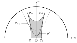
Figure 9. The shaded region is equal to $(\mathbf{T}_{a}\cap\Omega)\cap\mathbb{B}^{2}_{+}$. If $\Sigma^{\prime}\neq\Sigma$, then $\sigma^{\prime}=\Sigma^{\prime}\cap\mathbb{B}_{+}^{2}$ is the portion of some catenary $\sigma_{a^{\prime}}$ with $a^{\prime}<a_{c}$ and then $\Sigma^{\prime}$ is unstable.

Since $\Sigma^{\prime}\subset\mathbf{T}_{a}\cap\Omega$, we have $a^{\prime}\leqslant{}a$. We claim that if $a^{\prime}<a$, that is $\Sigma^{\prime}$ is not the same as $\Sigma$, then it must be unstable, which implies a contradiction. In fact, if $a^{\prime}<a$, since $\varrho(a^{\prime})<\varrho(a)<\varrho(a_{c})$, we have $a^{\prime}<a_{c}$ by Proposition 7.4, which implies that $\mathcal{C}_{a^{\prime}}$ is unstable. Besides, according to Proposition 7.5, the subdomain $\Sigma^{\prime}$ of $\mathcal{C}_{a^{\prime}}$ is also unstable since $\Sigma^{\prime}$ contains the maximal weakly stable domain of $\mathcal{C}_{a^{\prime}}$, so it couldn’t be a least area minimal surface unless $\Sigma^{\prime}\equiv\Sigma$.

Therefore any compact annulus of the form (5.5) is a least area minimal surface. ∎

Now let $S$ be any compact domain of $\mathcal{C}_{a}$, then we always can find a compact annulus $\Sigma$ of the form (5.5) such that $S\subset\Sigma$. If $S$ is not a least area minimal surface, then we can use the cutting and pasting technique to show that $\Sigma$ is not a least area minimal surface. This is contradicted to the above argument.

Therefore if $a\geqslant{}a_{l}$, then $\mathcal{C}_{a}$ is a least area minimal surface in the sense of Meeks and Yau. ∎

Remark 5.5.

In the proof of Claim 2 in Theorem 1.4, if $\Sigma^{\prime}$ is an annulus type minimal surface but it is not a least area minimal surface, then it might not be a surface of revolution (see [Lóp00, p. 234]).

Corollary 5.6.

There exists a finite constant $a_{l}\approx{}1.10055$ such that for two disjoint circles $C_{1},C_{2}\subset{}S_{\infty}^{2}$, if $d_{L}(C_{1},C_{2})\leqslant{}2\varrho(a_{l})\approx{}0.72918$, then there exist a least area spherical minimal catenoid $\mathcal{C}$ which is asymptotic to $C_{1}\cup{}C_{2}$, where the function $\varrho(a)$ is given by (3.20).

6. Stability of Helicoids

In this section, we will prove Theorem 1.5. One of the key points in the proof is that two conjugate minimal surfaces are either both stable or both unstable.

6.1. Conjugate minimal surface

Let $M^{3}(c)$ be the $3$-dimensional space form whose sectional curvature is a constant $c$.

Definition 6.1 ([dCD83, pp. 699-700]).

Let $f:\Sigma\to{}M^{3}(c)$ be a minimal surface in isothermal parametrs $(\sigma,t)$. Denote by

$$\operatorname{I}=E(d\sigma^{2}+dt^{2})\quad\text{and}\quad\operatorname{II}=\beta_{11}d\sigma^{2}+2\beta_{12}d\sigma{}dt+\beta_{22}dt^{2}$$

the first and second fundamental forms of $f$, respectively.

Set $\psi=\beta_{11}-i\beta_{12}$ and define a family of quadratic form depending on a parameter $\theta$, $0\leqslant\theta\leqslant{}2\pi$, by

$$\beta_{11}(\theta)=\mathop{\mathrm{Re}}(e^{i\theta}\psi)\ ,\quad\beta_{22}(\theta)=-\mathop{\mathrm{Re}}(e^{i\theta}\psi)\ ,\quad\beta_{12}(\theta)=\mathop{\mathrm{Im}}(e^{i\theta}\psi)\ .$$ (6.1)

Then the following forms

$$\operatorname{I}_{\theta}=\operatorname{I}\quad\text{and}\quad\operatorname{II}_{\theta}=\beta_{11}(\theta)d\sigma^{2}+2\beta_{12}(\theta)d\sigma{}dt+\beta_{22}(\theta)dt^{2}$$

give rise to an isometry family $f_{\theta}:\widetilde{\Sigma}\to{}M^{3}(c)$ of minimal immersions, where $\widetilde{\Sigma}$ is the universal covering of $\Sigma$. The immersion $f_{\pi/2}$ is called the conjugate immersion to $f_{0}=f$.

The following result is obvious, but it’s crucial to prove Theorem 1.4.

Lemma 6.2.

Let $f:\Sigma\to{}M^{3}(c)$ be an immersed minimal surface, and let $f_{\pi/2}:\widetilde{\Sigma}\to{}M^{3}(c)$ be its conjugate minimal surface, where $\widetilde{\Sigma}$ is the universal covering of $\Sigma$. Then the minimal immersion $f$ is globally stable if and only if its conjugate immersion $f_{\pi/2}$ is globally stable.

Proof.

Let $\widetilde{f}$ be the universal lifting of $f$, then $\widetilde{f}:\widetilde{\Sigma}\to{}M^{3}(c)$ is a minimal immersion. It’s well known that the global stability of $f$ implies the global stability of $\widetilde{f}$. Actually the minimal surfaces $\Sigma$ and $\widetilde{\Sigma}$ share the same Jacobi operator defined by (2.1). If $\Sigma$ is globally stable, there exists a positive Jacobi field on $\Sigma$ according to Theorem 2.3, which implies that $\widetilde{\Sigma}$ is also globally stable, since the corresponding positive Jacobi field on $\widetilde{\Sigma}$ is given by composing.

Next we claim that $\widetilde{f}$ and $f_{\pi/2}$ share the same Jacobi operator. In fact, since the Laplacian depends only on the first fundamental form, $\widetilde{f}$ and $f_{\pi/2}$ have the same Laplacian. Furthermore according to the definition of the conjugate minimal immersion, $\widetilde{f}$ and $f_{\pi/2}$ have the same square norm of the second fundamental form, i.e. $|A|^{2}=(\beta_{11}^{2}+2\beta_{12}^{2}+\beta_{22}^{2})/E^{2}$, where we used the notations in Definition 6.1.

By (2.1) and Theorem 2.3, the proof of the lemma is complete. ∎

6.2. Proof of Theorem 1.5

For hyperbolic and parabolic catenoids in $\mathbf{H}^{3}$ defined in $\S$2.3.2 and $\S$2.3.3, do Carmo and Dajczer proved that they are globally stable (see [dCD83, Theorem (5.5)]). Furthermore, Candel proved that the hyperbolic and parabolic catenoids are least area minimal surfaces (see [Can07, p. 3574]).

The following result will be used for proving Theorem 1.5. The equation (6.2) can be found in [BSE09, p. 34].

Lemma 6.3 (Bérard and Sa Earp).

The spherical catenoid $\mathscr{C}_{1}(\tilde{a})$ defined in $\S$2.3.1 is isometric to the spherical catenoid $\mathcal{C}_{a}$ defined in $\S$3.1, where

$$2\tilde{a}=\cosh(2a)\ .$$ (6.2)

Proof.

The spherical catenoid $\mathcal{C}_{a}$ is obtained by rotating the generating curve $\sigma_{a}$ along the axis $\gamma_{0}$ in (3.2). The distance between $\sigma_{a}$ and $\gamma_{0}$ is $a$.

The spherical catenoid $\mathscr{C}_{1}(\tilde{a})$ defined in $\S$2.3.1 can be obtained by rotating the generating curve $C$ given by (2.6) and (2.7) along the geodesic $P^{2}\cap\mathbf{H}^{3}$. The distance between $C$ and $P^{2}\cap\mathbf{H}^{3}$ is $\sinh^{-1}\left(\sqrt{\tilde{a}-1/2}\,\right)$.

Therefore the catenoid $\mathscr{C}_{1}(\tilde{a})$ is isometric to the catenoid $\mathcal{C}_{a}$ if and only if $a=\sinh^{-1}\left(\sqrt{\tilde{a}-1/2}\,\right)$, which implies (6.2). ∎

The following result can be found in [dCD83, Theorem (3.31)].

Theorem 6.4 (do Carmo-Dajczer).

Let $f:\mathscr{C}\to\mathbf{H}^{3}$ be a minimal catenoid defined in $\S$2.3. Its conjugate minimal surface is the geodesically-ruled minimal surface $\mathcal{H}_{\bar{a}}$ given by (2.14) where

$$\begin{cases}\bar{a}=\sqrt{(\tilde{a}+1/2)/(\tilde{a}-1/2)}\ ,&\text{if}\ \mathscr{C}=\mathscr{C}_{1}(\tilde{a})\ \text{is spherical}\ ,\\ \bar{a}=\sqrt{(\tilde{a}-1/2)/(\tilde{a}+1/2)}\ ,&\text{if}\ \mathscr{C}=\mathscr{C}_{-1}(\tilde{a})\ \text{is hyperbolic}\ ,\\ \bar{a}=1\ ,&\text{if}\ \mathscr{C}=\mathscr{C}_{0}\ \text{is parabolic}\ .\end{cases}$$ (6.3)

Now we are able to prove the theorem.

Theorem 1.5.

For a family of minimal helicoids $\{\mathcal{H}_{\bar{a}}\}_{\bar{a}\geqslant{}0}$ in the hyperbolic $3$-space given by (2.14), there exist a constant $\bar{a}_{c}=\coth(a_{c})\approx{}2.17968$ such that the following statements are true:

1. $\mathcal{H}_{\bar{a}}$ is a globally stable minimal surface if $0\leqslant{}\bar{a}\leqslant{}\bar{a}_{c}$, and

2. $\mathcal{H}_{\bar{a}}$ is an unstable minimal surface with Morse index one if $\bar{a}>\bar{a}_{c}$.

Proof.

When $\bar{a}=0$, $\mathcal{H}_{\bar{a}}$ is a hyperbolic plane, so it is globally stable.

According to Theorem 6.4, when $0<\bar{a}<1$, $\mathcal{H}_{\bar{a}}$ is conjugate to the hyperbolic catenoid $\mathscr{C}_{-1}(\tilde{a})$, where $\bar{a}=\sqrt{(\tilde{a}-1/2)/(\tilde{a}+1/2)}$ by (6.3), and when $\bar{a}=1$, $\mathcal{H}_{\bar{a}}$ is conjugate to the parabolic catenoid $\mathscr{C}_{0}$ in $\mathbf{H}^{3}$. Therefore when $0<\bar{a}\leqslant{}1$, the helicoid $\mathcal{H}_{\bar{a}}$ is globally stable by [dCD83, Theorem (5.5)].

When $\bar{a}>1$, $\mathcal{H}_{\bar{a}}$ is conjugate to the spherical catenoid $\mathscr{C}_{1}(\tilde{a})$ in $\mathbf{H}^{3}$ by Theorem 6.4, which is isometric to the spherical catenoid $\mathcal{C}_{a}$ in $\mathbb{B}^{3}$, where $2\tilde{a}=\cosh(2a)$ by (6.2) and $\bar{a}=\sqrt{(\tilde{a}+1/2)/(\tilde{a}-1/2)}$ by (6.3). Therefore $\mathcal{H}_{\bar{a}}$ is conjugate to the spherical catenoid $\mathcal{C}_{a}$ in $\mathbb{B}^{3}$, where

$$\bar{a}=\coth(a)\ .$$

By Theorem 1.2, the catenoid $\mathcal{C}_{a}$ is globally stable if $a\geqslant{}a_{c}\approx{}0.49577$, therefore $\mathcal{H}_{\bar{a}}$ is globally stable when $1<\bar{a}\leqslant{}\bar{a}_{c}=\coth(a_{c})\approx{}2.17968$.

On the other hand, if $0<a<a_{c}$, then the catenoid $\mathcal{C}_{a}$ is unstable with Morse index one by Theorem 1.2, therefore $\mathcal{H}_{\bar{a}}$ is unstable when $\bar{a}>\bar{a}_{c}$.

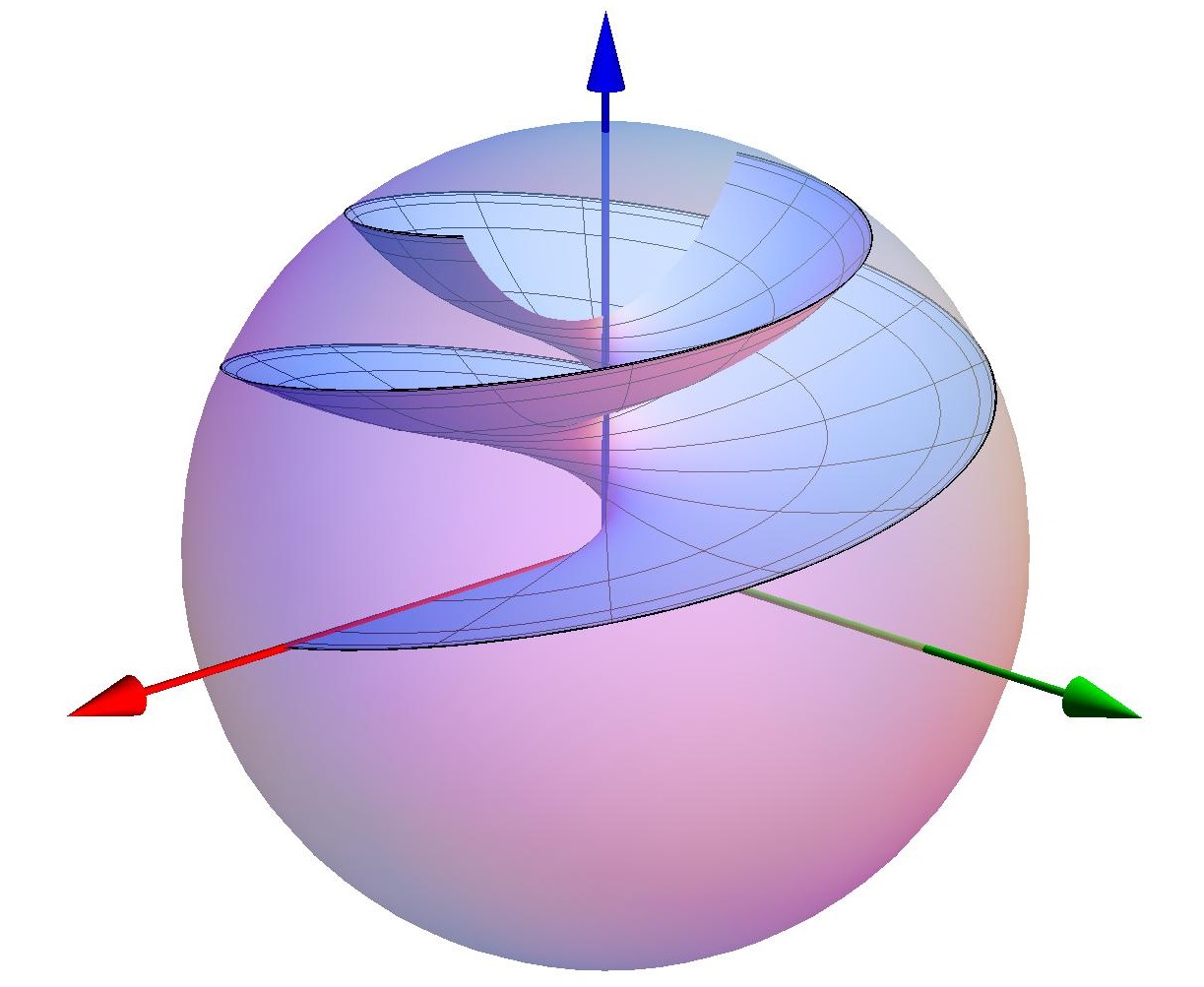
Figure 10. This is a subdomain of the helicoid $\mathcal{H}_{5}\subset\mathbb{B}^{3}$ between two geodesics $v=0$ and $v=\pi/\sqrt{6}$ of $\mathcal{H}_{5}$, which is isometric to the fundamental domain of the universal cover of the catenoid $\mathcal{C}_{a}$ for $a=\coth^{-1}(5)$.

At last we will show that the Morse index of the helicoid $\mathcal{H}_{\bar{a}}$ for $\bar{a}>\bar{a}_{c}$ is infinite. Otherwise according to Theorem 2.4, there is a compact subdomain $K$ of $\mathcal{H}_{\bar{a}}$ such that $\mathcal{H}_{\bar{a}}\setminus{}K$ is stable. But this is impossible, since we always can find a (noncompact) subdomain $\mathcal{U}$ of $\mathcal{H}_{\bar{a}}$ as follows: Consider the parametric equation (2.15) of $\mathcal{H}_{\bar{a}}$ in the Poincaré ball model $\mathbb{B}^{3}$ of the hyperbolic $3$-space, and write $\mathcal{U}$ by

$$\mathcal{U}=\left\{(x,y,z)\in\mathcal{H}_{\bar{a}}\ |\ u\in\mathbb{R}\ \text{and}\ v_{0}\leqslant{}v\leqslant{}v_{0}+2\pi\sinh(\coth^{-1}(\bar{a}))\right\}\ ,$$

where $v_{0}>0$ is sufficiently large such that $K$ is underneath the geodesic of $\mathbb{B}^{3}$ which passes through the point $(0,0,\tanh(v_{0}/2))\in\mathbb{B}^{3}$ and is contained in $\mathcal{H}_{\bar{a}}$ (see Figure 10). It’s easy to verify that

• $\mathcal{U}$ is disjoint from $K$, i.e. $\mathcal{U}\subset\mathcal{H}_{\bar{a}}\setminus{}K$, and

• $\mathcal{U}$ is isometric to the fundamental domain of the universal cover of the catenoid $\mathcal{C}_{a}$, where $a=\coth^{-1}(\bar{a})<a_{c}$.

Therefore $\mathcal{U}$ is unstable, and so is $\mathcal{H}_{\bar{a}}\setminus{}K$. ∎

7. Technical Lemmas

7.1. Lemmas for $\S$4

In this part, we prove Lemma 7.1 and Lemma 7.2, which will be applied to prove Theorem 1.2.

Lemma 7.1.

Let $\phi(a,t)=\sqrt{5}\,\cosh(a+t)-\cosh(3a+t)$, then $\phi(a,t)\leqslant{}0$ for $(a,t)\in{}[A_{3},\infty)\times[0,\infty)$, where the constant $A_{3}$ is defined by

$$A_{3}=\cosh^{-1}\left(\frac{\sqrt{3+\sqrt{5}}}{2}\right)\approx 0.530638\ .$$ (7.1)

Proof.

It’s easy to verify that $\phi(a,t)\leqslant{}0$ is equivalent to

$$\cosh(3a)-\sqrt{5}\cosh{}a+\tanh{}t\cdot(\sinh(3a)-\sqrt{5}\sinh{}a)\geqslant{}0\ .$$

Since $\tanh{}t\geqslant{}0$ for $t\geqslant{}0$ and $\sinh(3a)-\sqrt{5}\sinh{}a\geqslant{}0$ for $a\geqslant{}0$, we need solve the inequality $\cosh(3a)-\sqrt{5}\cosh{}a\geqslant{}0$.

Let $A_{3}$ be the solution of the equation $0=\sqrt{5}\,\cosh{}a-\cosh(3a)=(\sqrt{5}-(4\cosh^{2}a-3))\cosh{}a$, then $\phi(a,t)\leqslant{}0$ if $a\geqslant{}A_{3}$ and $t\geqslant{}0$. ∎

Lemma 7.2.

Let $\psi(a,t)$ be the function given by

$$\psi(a,t)= \,76\sinh(2a)-22\sinh(2t)+29\sinh(4a+2t)$$ (7.2)

$$\,+\sinh(8a+2t)-26\sinh(6a+4t)-6\sinh(10a+4t)$$

$$\,-25\sinh(8a+6t)+\sinh(12a+6t)\ .$$

Then $\psi(a,t)<0$ for all $(a,t)\in{}[0,A_{4}]\times[0,\infty)$, where the constant

$$A_{4}=\frac{1}{4}\cosh^{-1}\left(\frac{35+\sqrt{1241}}{8}\right)\approx 0.715548$$ (7.3)

is the solution of the equation $4\cosh^{2}(4a)-35\cosh(4a)-1=0$.

Proof.

Expand each term in $\psi(a,t)$ with the form $\sinh(ma+nt)$ , then we may write $\psi(a,t)=\psi_{1}(a,t)+\psi_{2}(a,t)$, where

$$\psi_{1}(a,t)= \,-22\sinh(2t)+29\sinh(2t)\cosh(4a)+\sinh(2t)\cosh(8a)$$

$$\,-26\sinh(4t)\cosh(6a)-6\sinh(4t)\cosh(10a)$$

$$\,-25\sinh(6t)\cosh(8a)+\sinh(6t)\cosh(12a))\ ,$$

and

$$\psi_{2}(a,t)= \,76\sinh(2a)+29\cosh(2t)\sinh(4a)+\cosh(2t)\sinh(8a)$$

$$\,-26\cosh(4t)\sinh(6a)-6\cosh(4t)\sinh(10a)$$

$$\,-25\cosh(6t)\sinh(8a)+\cosh(6t)\sinh(12a)\ .$$

Claim: $\psi_{1}(a,t)\leqslant{}0$ and $\psi_{2}(a,t)\leqslant{}0$ for $(a,t)\in[0,A_{4}]\times[0,\infty)$.

Proof of Claim.

First of all, we will show that $\psi_{1}(a,\cdot)\leqslant{}0$ for $a\in[0,A_{4}]$. Since $\cosh(2t)\geqslant{}1$ for any $t\in[0,\infty)$, we have the estimate

$$\psi_{1}(a,t)= \,-\sinh(2t)(22-29\cosh(4a)-\cosh(8a)$$

$$\qquad\qquad+52\cosh(2t)\cosh(6a)+12\cosh(2t)\cosh(10a))$$

$$\,-\sinh(6t)(25\cosh(8a)-\cosh(12a))$$

$$\leqslant \,-\sinh(2t)(22-29\cosh(4a)-\cosh(8a)$$

$$\qquad\qquad+52\cosh(6a)+12\cosh(10a))$$

$$\,-\sinh(6t)(25\cosh(8a)-\cosh(12a))\ .$$

Since $52\cosh(6a)-29\cosh(4a)>0$ and $12\cosh(10a)-\cosh(8a)>0$ for $0\leqslant{}a<\infty$ and $25\cosh(8a)-\cosh(12a)>0$ for $0\leqslant{}a\leqslant{}A_{4}$, we have $\psi_{1}(a,\cdot)<0$ for $0\leqslant{}a\leqslant{}A_{4}$.

Secondly, for any $a\geqslant{}0$, we apply the inequality

$$\sinh((m+n)a)\geqslant\sinh(ma)+\sinh(na)\ ,$$

where $m,n$ are positive integers, to get the following inequalities

• $\sinh(6a)\geqslant\sinh(4a)+\sinh(2a)$,

• $\sinh(8a)\geqslant{}4\sinh(2a)$, and

• $\displaystyle\sinh(10a)\geqslant\begin{cases}\sinh(8a)+\sinh(2a)\\ \sinh(4a)+3\sinh(2a)\\ 5\sinh(2a)\end{cases}$ ,

which can imply the estimate

$$\psi_{2}(a,t)\leqslant \,-46\sinh(2a)(\cosh(4t)-1)-30\sinh(2a)(\cosh(6t)-1)$$

$$\,-29\sinh(4a)(\cosh(4t)-\cosh(2t))$$

$$\,-\sinh(8a)(\cosh(4t)-\cosh(2t))$$

$$\,-\cosh(6t)\left(\frac{35}{2}\sinh(8a)-\sinh(12a)\right)\ .$$

As $\frac{35}{2}\sinh(8a)-\sinh(12a)=\sinh(4a)(1+35\cosh(4a)-4\cosh^{2}(4a))\geqslant{}0$ if $0\leqslant{}a\leqslant{}A_{4}$ and the fact $\cosh(6t)\geqslant\cosh(4t)\geqslant\cosh(2t)\geqslant{}1$ for $0\leqslant{}t<\infty$, we have $\psi_{2}(a,t)\leqslant{}0$ for $(a,t)\in[0,A_{4}]\times[0,\infty)$. ∎

Therefore $\psi(a,t)<0$ for $(a,t)\in[0,A_{4}]\times[0,\infty)$. ∎

7.2. Lemmas for $\S$5

In this subsection, we will prove Proposition 7.4 and Proposition 7.5, which will be used to prove Theorem 1.4. At first, we need the following lemma.

Lemma 7.3.

Let $R_{3}$ and $R_{4}$ be the regions defined by

$$R_{3} =\{(a,t)\in\mathbb{R}^{2}\ |\ t\geqslant{}a\geqslant{}A_{3}\}\ ,$$

$$R_{4} =\{(a,t)\in\mathbb{R}^{2}\ |\ 0<a\leqslant{}A_{4}\ \text{and}\ t\geqslant{}a\}\ ,$$

where $A_{3}$ and $A_{4}$ are the constants defined in (7.1) and (7.3). Then we have

$$\frac{\partial{}}{\partial{a}}\,\rho(a,t)<0\quad\text{for}\ (a,t)\in{}R_{3}\ ,$$

and

$$\frac{\partial^{2}{}}{\partial{a}^{2}}\,\rho(a,t)<0\quad\text{for}\ (a,t)\in{}R_{4}\ ,$$

where $\rho(a,t)$ is defined in (3.9^′).

Proof.

Using the substitution $\tau\mapsto\tau+a$ in (3.9^′), we have

$$\rho(a,t)=\int_{0}^{t-a}\frac{\sinh(2a)}{\cosh(a+\tau)}\frac{d\tau}{\sqrt{\sinh^{2}(2a+2\tau)-\sinh^{2}(2a)}}\ ,\quad{}t\geqslant{}a\ .$$

Direct computation shows

$$\frac{\partial{}}{\partial{a}}\,\rho(a,t)= \,\int_{0}^{t-a}\frac{\sinh(a+\tau)(5\cosh^{2}(a+\tau)-\cosh^{2}(3a+\tau))}{\cosh^{2}(a+\tau)\sqrt{\sinh(2\tau)\sinh^{3}(4a+2\tau)}}\,d\tau$$

$$-\frac{\sinh(2a)}{\cosh{}t\cdot\sqrt{\sinh^{2}(2t)-\sinh^{2}(2a)}}$$

and

$$\frac{\partial^{2}{}}{\partial{a}^{2}}\,\rho(a,t)= \,\int_{0}^{t-a}\frac{\psi(a,\tau)}{16\cosh^{3}(a+\tau)\sqrt{\sinh(2\tau)\sinh^{5}(4a+2\tau)}}\,d\tau$$

$$\,-\frac{\sinh{}t\cdot{}w(a,t)}{\sqrt{2}\,\cosh^{2}t\cdot(\cosh(4t)-\cosh(4a))^{3/2}}\ ,$$

where $\psi(a,\tau)$ is given by (7.2) and $w(a,t)$ is defined by

$$w(a,t)= \,-5\sinh(2a)+\sinh(6a)-7\sinh(2a-4t)$$

$$\,-12\sinh(2a-2t)+4\sinh(2a+2t)+\sinh(2a+4t)\ .$$

Recall that $t\geqslant{}a>0$, we have $w(a,t)\geqslant\sinh(6a)>0$, together with the arguments in the proofs of Lemma 7.1 and Lemma 7.2, the proof of the lemma is complete. ∎

Proposition 7.4 ([BSE10, Proposition 4.8 and Lemma 4.9]).

Let $\sigma_{a}\subset\mathbb{B}_{+}^{2}$ be the catenary given by (3.9). For $0<a_{1}<a_{2}$, the catenaries $\sigma_{a_{1}}$ and $\sigma_{a_{2}}$ intersect at most at two symmetric points and they do so if and only if $\varrho(a_{1})<\varrho(a_{2})$. Furthermore we have the following results:

1. For $a_{1},a_{2}\in(0,a_{c})$, the catenaries $\sigma_{a_{1}}$ and $\sigma_{a_{2}}$ intersect exactly at two symmetric points (see Figure 12).

2. All catenaries in the family $\{\sigma_{a}\ |\ a\geqslant{}a_{c}\}$ foliate the subdomain of $\mathbb{B}^{2}_{+}$ that is bounded by the catenary $\sigma_{a_{c}}$ and the arc of $\partial_{\infty}\mathbb{B}^{2}_{+}$ between the asymptotic boundary points of $\sigma_{a_{c}}$ (see Figure 12).

Proof.

For $0<a_{1}<a_{2}$, we define a function

$$\delta(t)=\rho(a_{2},t)-\rho(a_{1},t)\ ,\quad{}t\geqslant{}a_{2}>a_{1}\ ,$$

where $\rho$ is defined by (3.9^′).

We claim that $\delta(t)$ is an increasing function on $[a_{2},\infty)$. Actually the derivative of $\delta(t)$ is given by the following expression

$$\delta^{\prime}(t)=\frac{1}{\cosh{}t}\left\{\frac{1}{\sqrt{\left(\dfrac{\sinh(2t)}{\sinh(2a_{2})}\right)^{2}-1}}-\frac{1}{\sqrt{\left(\dfrac{\sinh(2t)}{\sinh(2a_{1})}\right)^{2}-1}}\right\}>0\ ,$$

on $[a_{2},\infty)$.

Since $\delta(0)=-\rho(a_{2},a_{1})<0$ and $\delta(\infty)=\varrho(a_{2})-\varrho(a_{1})$, we have the conclusion that the catenaries $\sigma_{a_{1}}$ and $\sigma_{a_{2}}$ intersect at most at two symmetric points and they do so if and only if $\varrho(a_{1})<\varrho(a_{2})$.

Statement (1) is true since $\varrho(a)$ is increasing on $(0,a_{c})$, and Statement (2) is true since $\varrho(a)$ is decreasing on $[a_{c},\infty)$ ∎

Figure 11. The family of catenaries for unstable catenoids.

Figure 12. The family of catenaries for stable catenoids.

An envelope of a family of curves in the hyperbolic plane is a curve that is tangent to each member of the family at some point. A point on the envelope can be considered as the intersection of two “adjacent” curves, meaning the limit of intersections of nearby curves.

According to Proposition 7.4, the catenaries $\sigma_{a_{1}}$ and $\sigma_{a_{2}}$ intersect exactly at two symmetric points if $0<a_{1}<a_{2}<a_{c}$. In order to prove Theorem 1.4, we should show that the family of catenaries $\{\sigma_{a}\}_{0<a<a_{c}}$ forms an envelope which is outside the region of $\mathbb{B}^{2}_{+}$ foliated by the family of catenaries $\{\sigma_{a}\}_{a\geqslant{}a_{c}}$, since each point in the envelope is corresponding to the boundary of the maximal weakly stable domain of some catenoid $\mathcal{C}_{a}$ for $0<a<a_{c}$.

Recall that the the numbers $\pm{}z(a)$ denote the only zeros of the variation field $\xi(a,s)$ on the catenoid $\mathcal{C}_{a}$ defined by (4.6) or (4.7) for each $0<a<a_{c}$.

Proposition 7.5 ([BSE10, Proposition 4.8 (2)]).

The family of catenaries $\{\sigma_{a}\ |\ 0<a<a_{c}\}$ defined in $\S$3.1.2 has an envelope, and the points at which $\sigma_{a}$ touches the envelope correspond to the maximal weakly stable domain $\mathcal{C}(z(a))$ defined by (4.12). Furthermore for any constant $a\in(0,a_{c})$ we have

$$\mathcal{C}(z(a))\cap\Bigg{(}\bigcup_{\alpha\geqslant{}a_{c}}\mathcal{C}_{\alpha}\Bigg{)}=\emptyset\ .$$ (7.4)

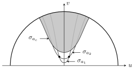
Figure 13. $\mathcal{D}$ is the shadow region. In this figure, $a_{1}=0.1$ and $a_{2}=0.25$. We can see that $\sigma_{a_{1}}\cap\sigma_{a_{2}}$ is disjoint from $\mathcal{D}$.

Proof.

For each $a\in(0,a_{c})$, the catenoid $\mathcal{C}_{a}$ and its maximal weakly stable domain $\mathcal{C}(z(a))$ are surfaces of revolution, so we just need to consider the $2$-dimensional case. Let

$$\mathcal{D}=\bigcup_{a\geqslant{}a_{c}}\sigma_{a}$$

be the subregion of $\mathbb{B}_{+}^{2}$. We will prove the proposition by three claims.

Claim 1.

$\sigma_{a_{1}}\cap\sigma_{a_{2}}$ is disjoint from $\mathcal{D}$ for $0<a_{1}<a_{2}<a_{c}$.

Proof of Claim 1.

See Figure 13. Actually if $\sigma_{a_{1}}\cap\sigma_{a_{2}}\subset{}\mathcal{D}$, since $\mathcal{D}$ is foliated by the catenaries $\{\sigma_{\alpha}\}_{\alpha\geqslant{}a_{c}}$, there exists $a_{3}>a_{c}$ such that $\sigma_{a_{1}}$, $\sigma_{a_{2}}$ and $\sigma_{a_{3}}$ intersect at the same points. Let $t_{0}$ be the $y$-coordinate of the intersection points (recall that we equip $\mathbb{B}^{2}_{+}$ with the warped product metric (3.6)), then $t_{0}>a_{3}$ (see the proof of Lemma 4.9 in [BSE10]). Consider the function

$$\varphi(\alpha)=\rho(\alpha,t_{0})\ ,\quad{}\alpha\in[a_{1},a_{3}]\ ,$$

where $\rho(a,t)$ is defined by (3.9^′).

By our assumption, $\varphi(a_{1})=\varphi(a_{2})=\varphi(a_{3})$. By L’Hôpital’s rule, there exist $a_{4}\in(a_{1},a_{2})$ and $a_{5}\in(a_{2},a_{3})$ such that $\varphi^{\prime}(a_{4})=\varphi^{\prime}(a_{5})=0$. By Lemma 7.3, $a_{5}<A_{3}$ and then $a_{5}<A_{4}$. Applying L’Hôpital’s rule again, there exists $a_{6}\in(a_{4},a_{5})\subset(a_{1},a_{3})\cap(0,A_{4})$ such that $\varphi^{\prime\prime}(a_{6})=0$. This is impossible according to Lemma 7.3. Therefore $\sigma_{a_{1}}\cap\sigma_{a_{2}}$ is disjoint from $\mathcal{D}$ for $0<a_{1}<a_{2}<a_{c}$. ∎

Claim 2.

For any $a\in(0,a_{c})$, there exist two symmetric points $p_{a}^{\pm}\subset\sigma_{a}$ disjoint from $\mathcal{D}$ such that

$$\lim\limits_{\alpha\to{}a}(\sigma_{a}\cap\sigma_{\alpha})=\{p_{a}^{\pm}\}\ .$$ (7.5)

Proof of Claim 2.

For $0<a_{1}<a_{2}<a_{3}<a_{c}$, let $y_{ij}$ denote the $y$-coordinate of the intersection of $\sigma_{a_{i}}$ and $\sigma_{a_{j}}$ ($1\leqslant{}i<j\leqslant{}3$), then we have $y_{12}<y_{13}<y_{23}$ (see Figure 14).

Figure 14. For $0<a_{i}<a_{j}<a_{c}$, let $y_{ij}$ denote the $y$-coordinate of the (symmetric) points $\sigma_{a_{i}}\cap\sigma_{a_{j}}$. In this figure, $a_{1}=0.1$, $a_{2}=0.2$ and $a_{3}=0.35$, and one can see that $y_{12}<y_{13}<y_{23}$.

Otherwise, we must have $y_{23}<y_{13}<y_{12}$, this may imply there exists $a_{4}\in(a_{3},a_{c})$ such that $\sigma_{a_{1}}$, $\sigma_{a_{2}}$ and $\sigma_{a_{4}}$ intersect at the same points. But this is impossible according to the similar argument as in Claim 1.

Therefore as $\alpha\to{}a^{+}$, the $y$-coordinates of $\sigma_{a}\cap\sigma_{\alpha}$ are decreasing, whereas as $\alpha\to{}a^{-}$, the $y$-coordinates of $\sigma_{a}\cap\sigma_{\alpha}$ are increasing, which can imply that $\lim\limits_{\alpha\to{}a}(\sigma_{a}\cap\sigma_{\alpha})$ exists, and the points $\{p_{a}^{\pm}\}$ are disjoint from $\mathcal{D}$ because of the statement in Claim 1. ∎

By Claim 1 and Claim 2, we actually have proved that the catenaries $\{\sigma_{a}\}_{0<a<a_{c}}$ has an envelope curve, denoted by

$$\Gamma=\{p_{a}^{\pm}\ |\ 0<a<a_{c}\}\cup\{(0,0)\}\ ,$$

which is disjoint from the region $\mathcal{D}$ (see Figure 15).

Recall that each catenary $\sigma_{a}$ can be parametrized by arc length as follows:

$$s\mapsto(x(a,s),y(a,s))$$

for $-\infty<s<\infty$, where $x(\cdot,\cdot)$ and $y(\cdot,\cdot)$ are defined by the equations (3.12) and (3.13) respectively. For each $a\in(0,a_{c})$, suppose that

$$p_{a}^{\pm}=(\pm{}x(a,s_{a}),y(a,s_{a}))\ .$$

Claim 3.

For any $a\in(0,a_{c})$, we have $z(a)=s_{a}$, where $\pm{}z(a)$ are the only zeros of the variation field $\xi(a,\cdot)$ given by (4.6) and (4.7).

Proof of Claim 3.

By the property of the envelope curve $\Gamma$, it is tangent to each catenary $\sigma_{a}$ at the points $p_{a}^{\pm}$ for $0<a<a_{c}$. Thus $\sigma_{a}$ and $\Gamma$ have the same tangent line at either $p_{a}^{+}$ or $p_{a}^{-}$.

The tangent vector to the catenary $\sigma_{a}$ at $p_{a}^{+}$ is $(x_{s}(a,s_{a}),y_{s}(a,s_{a}))$, and the tangent vector to the envelope $\Gamma$ at $p_{a}^{+}$ is $(x_{a}(a,s_{a}),y_{a}(a,s_{a}))$. These two vectors must be proportional, therefore we have

$$x_{a}(a,s_{a})y_{s}(a,s_{a})-x_{s}(a,s_{a})y_{a}(a,s_{a})=0$$

for all $0<a<a_{c}$. Now by (4.6), the variation field $\xi(a,s)$ on the catenoid $\mathcal{C}_{a}$ has two symmetric zeros at $s_{a}$ and $-s_{a}$. On the other hand, according to Lemma 4.5, these are the only zeros of $\xi(a,s)$ for $s\in(-\infty,\infty)$. Thus we have $z(a)=s_{a}$ for all $0<a<a_{c}$. ∎

Now according to Claim 3, we have (7.4), and then the proof of the whole proposition is complete. ∎

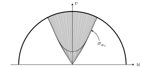
Figure 15. $\mathcal{D}$ is the shadow region. The family of catenaries $\sigma_{a}$ for $0<a<a_{c}$ forms an envelope curve, which is disjoint from $\mathcal{D}$.

References

- [BdC80] João Lucas Barbosa and Manfredo do Carmo, Stability of minimal surfaces in spaces of constant curvature, Bol. Soc. Brasil. Mat. 11 (1980), no. 1, 1–10.
- [BdCH09] Allen Back, Manfredo do Carmo, and Wu-Yi Hsiang, On some fundamental equations of equivariant Riemannian geometry, Tamkang J. Math. 40 (2009), no. 4, 343–376.
- [Bea95] Alan F. Beardon, The geometry of discrete groups, Graduate Texts in Mathematics, vol. 91, Springer-Verlag, New York, 1995, Corrected reprint of the 1983 original.
- [BP92] Riccardo Benedetti and Carlo Petronio, Lectures on hyperbolic geometry, Universitext, Springer-Verlag, Berlin, 1992.
- [BSE09] Pierre Bérard and Ricardo Sa Earp, Lindelöf’s theorem for catenoids revisited, arXiv:0907.4294v1 (2009).
- [BSE10] by same author, Lindelöf’s theorem for hyperbolic catenoids, Proc. Amer. Math. Soc. 138 (2010), no. 10, 3657–3669.
- [Can07] Alberto Candel, Eigenvalue estimates for minimal surfaces in hyperbolic space, Trans. Amer. Math. Soc. 359 (2007), no. 8, 3567–3575 (electronic).
- [CG06] Danny Calegari and David Gabai, Shrinkwrapping and the taming of hyperbolic 3-manifolds, J. Amer. Math. Soc. 19 (2006), no. 2, 385–446.
- [CM11] Tobias Holck Colding and William P. Minicozzi, II, A course in minimal surfaces, Graduate Studies in Mathematics, vol. 121, American Mathematical Society, Providence, RI, 2011.
- [dCD83] Manfredo do Carmo and Marcos Dajczer, Rotation hypersurfaces in spaces of constant curvature, Trans. Amer. Math. Soc. 277 (1983), no. 2, 685–709.
- [dCGT86] Manfredo do Carmo, Jonas de Miranda Gomes, and Gudlaugur Thorbergsson, The influence of the boundary behaviour on hypersurfaces with constant mean curvature in , Comment. Math. Helv. 61 (1986), no. 3, 429–441.
- [dCP79] M. do Carmo and C. K. Peng, Stable complete minimal surfaces in are planes, Bull. Amer. Math. Soc. (N.S.) 1 (1979), no. 6, 903–906.
- [dOS98] Geraldo de Oliveira and Marc Soret, Complete minimal surfaces in hyperbolic space, Math. Ann. 311 (1998), no. 3, 397–419.
- [FC85] D. Fischer-Colbrie, On complete minimal surfaces with finite Morse index in three-manifolds, Invent. Math. 82 (1985), no. 1, 121–132.
- [FCS80] Doris Fischer-Colbrie and Richard Schoen, The structure of complete stable minimal surfaces in -manifolds of nonnegative scalar curvature, Comm. Pure Appl. Math. 33 (1980), no. 2, 199–211.
- [FT91] Anatoliĭ T. Fomenko and Alexey A. Tuzhilin, Elements of the geometry and topology of minimal surfaces in three-dimensional space, Translations of Mathematical Monographs, vol. 93, American Mathematical Society, Providence, RI, 1991, Translated from the Russian by E. J. F. Primrose.
- [Gom87] Jonas de Miranda Gomes, Spherical surfaces with constant mean curvature in hyperbolic space, Bol. Soc. Brasil. Mat. 18 (1987), no. 2, 49–73.
- [Hsi82] Wu-yi Hsiang, On generalization of theorems of A. D. Alexandrov and C. Delaunay on hypersurfaces of constant mean curvature, Duke Math. J. 49 (1982), no. 3, 485–496.
- [HW15] Zheng Huang and Biao Wang, Counting minimal surfaces in quasi-Fuchsian three-manifolds, Trans. Amer. Math. Soc. 367 (2015), no. 9, 6063–6083.
- [Lóp00] Rafael López, Hypersurfaces with constant mean curvature in hyperbolic space, Hokkaido Math. J. 29 (2000), no. 2, 229–245.
- [LR85] Gilbert Levitt and Harold Rosenberg, Symmetry of constant mean curvature hypersurfaces in hyperbolic space, Duke Math. J. 52 (1985), no. 1, 53–59.
- [LR89] Francisco J. López and Antonio Ros, Complete minimal surfaces with index one and stable constant mean curvature surfaces, Comment. Math. Helv. 64 (1989), no. 1, 34–43.
- [LR91] by same author, On embedded complete minimal surfaces of genus zero, J. Differential Geom. 33 (1991), no. 1, 293–300.
- [Mor81] Hiroshi Mori, Minimal surfaces of revolution in and their global stability, Indiana Univ. Math. J. 30 (1981), no. 5, 787–794.
- [Mor82] by same author, On surfaces of right helicoid type in , Bol. Soc. Brasil. Mat. 13 (1982), no. 2, 57–62.
- [MP11] William H. Meeks, III and Joaquín Pérez, The classical theory of minimal surfaces, Bull. Amer. Math. Soc. (N.S.) 48 (2011), no. 3, 325–407.
- [MP12] by same author, A survey on classical minimal surface theory, University Lecture Series, vol. 60, American Mathematical Society, Providence, RI, 2012.
- [MR05] William H. Meeks, III and Harold Rosenberg, The uniqueness of the helicoid, Ann. of Math. (2) 161 (2005), no. 2, 727–758.
- [MT98] Katsuhiko Matsuzaki and Masahiko Taniguchi, Hyperbolic manifolds and Kleinian groups, Oxford Mathematical Monographs, The Oxford University Press, New York, 1998.
- [MY82a] William W. Meeks, III and Shing Tung Yau, The classical Plateau problem and the topology of three-dimensional manifolds. The embedding of the solution given by Douglas-Morrey and an analytic proof of Dehn’s lemma, Topology 21 (1982), no. 4, 409–442.
- [MY82b] by same author, The existence of embedded minimal surfaces and the problem of uniqueness, Math. Z. 179 (1982), no. 2, 151–168.
- [Sch83] Richard M. Schoen, Uniqueness, symmetry, and embeddedness of minimal surfaces, J. Differential Geom. 18 (1983), no. 4, 791–809 (1984).
- [Seo11] Keomkyo Seo, Stable minimal hypersurfaces in the hyperbolic space, J. Korean Math. Soc. 48 (2011), no. 2, 253–266.
- [Tuz93] Alexey A. Tuzhilin, Global properties of minimal surfaces in and and their Morse type indices, Minimal surfaces, Adv. Soviet Math., vol. 15, Amer. Math. Soc., Providence, RI, 1993, pp. 193–233.
- [Wan12] Biao Wang, Minimal surfaces in quasi-Fuchsian 3-manifolds, Math. Ann. 354 (2012), no. 3, 955–966.
- [Xin03] Yuanlong Xin, Minimal submanifolds and related topics, Nankai Tracts in Mathematics, vol. 8, World Scientific Publishing Co. Inc., River Edge, NJ, 2003.