Kink-antikink asymmetry and impurity interactions in topological mechanical chains

Abstract

We study the dynamical response of a diatomic periodic chain of rotors coupled by springs, whose unit cell breaks spatial inversion symmetry. In the continuum description, we derive a nonlinear field theory which admits topological kinks and antikinks as nonlinear excitations but where a topological boundary term breaks the symmetry between the two and energetically favors the kink configuration. Using a cobweb plot, we develop a fixed-point analysis for the kink motion and demonstrate that kinks propagate without the Peierls-Nabarro potential energy barrier typically associated with lattice models. Using continuum elasticity theory, we trace the absence of the Peierls-Nabarro barrier for the kink motion to the topological boundary term which ensures that only the kink configuration, and not the antikink, costs zero potential energy. Further, we study the eigenmodes around the kink and antikink configurations using a tangent stiffness matrix approach appropriate for pre-stressed structures to explicitly show how the usual energy degeneracy between the two no longer holds. We show how the kink-antikink asymmetry also manifests in the way these nonlinear excitations interact with impurities introduced in the chain as disorder in the spring stiffness. Finally, we discuss the effect of impurities in the (bond) spring length and build prototypes based on simple linkages that verify our predictions.

I Introduction

Topological ideas have led to recent advances in continuum mechanics often inspired by the physics of electronic topological insulators and the quantum Hall effect. In these electronic systems the basic question is whether a material is an insulator or a conductor. The answer depends on which portion of a topological insulator one examines: the bulk is usually gapped and hence insulating while the edge displays gapless edge modes whose existence is protected from disorder and variations in material parameters by the existence of integer-valued topological invariants Hasan and Kane (2010). In topological mechanical systems, the corresponding question is whether a material is rigid or floppy. The ability to modulate the rigidity of a structure in space allows to robustly localize the propagation of sound waves Prodan and Prodan (2009); Berg et al. (2011); Susstrunk and Huber (2015); Süsstrunk and Huber (2016); Wang et al. (2015a, b); Mousavi et al. (2015); Khanikaev et al. (2015); Nash et al. (2015); Yang et al. (2015a, b); Xiao et al. (2015); Peano et al. (2015); Kariyado and Hatsugai (2015); Deymier et al. (2015); Bi and Wang (2015); Po et al. (2014); Lawler (2015), change shape in selected portions Kane and Lubensky (2013); Lubensky et al. (2015); Vitelli (2012); Chen et al. (2014); Vitelli et al. (2014); Meeussen et al. (2016); Paulose et al. (2015a); Chen et al. (2016); Rocklin et al. (2015, 2016) or focus stress leading to selective buckling or failure Paulose et al. (2015b).

By translating the topological properties of bands of electronic states into the classical setting of vibrational bands, one can identify topologically protected and hence robust properties of vibrational modes in both discrete lattices and continuous media. For example, the concept of “topological polarization” recently introduced by Kane and Lubensky Kane and Lubensky (2013) building on counting ideas from Maxwell and Calladine  Maxwell (1864); Calladine (1978) determines the existence and the position of zero-energy motions that are localized at edges and defects of a marginally rigid mechanical lattice (one in which constraints and degrees of freedom are exactly balanced).

Perhaps the simplest model of topological mechanical lattices is the rotor chain proposed in Ref. Kane and Lubensky (2013). The system consists of a chain of classical rotors harmonically coupled with their nearest neighbours, as shown in Fig. 1a. There are two distinct classes of ground state configurations, one with all rotors leaning towards the left and the other where they lean towards the right. Mathematically, these two states may not be deformed to each other without the appearance of bulk zero modes; thus they may each be assigned a different winding number, associated with the Fourier transform of the compatibility matrix $C(q)$, which connects the linear displacement of rotors with the extension of bonds; see Ref. Lubensky et al. (2015) for a detailed explanation.

The above considerations arise from band theory and thus concern only the linearized zero-energy infinitesimal motions. Indeed, the vanishing of the linear response implies that nonlinear effects dominate. By developing a nonlinear theory of the rotor chain, it was shown in Ref. Chen et al. (2014) that the infinitesimal zero-mode displacement integrates to a finite motion. This motion can be described in the continuum limit by objects similar to “kinks” in the $\phi^{4}$ field theory  Manton and Sutcliffe (2004), which connects the topological polarization invariant of the linear vibrations to the study of topological solitons  Chen et al. (2014); Vitelli et al. (2014). Although the two appearances of the term “topology” in the linear and nonlinear theory stem from different contexts, the latter encompasses the predictions of the former and also explains additional features exclusive to the nonlinear dynamics  Vitelli et al. (2014).

The nonlinear dynamics of this topological chain can be approximated by the critical trajectories of a Lagrangian written in the following form  Chen et al. (2014); Vitelli et al. (2014)

$$\begin{split}L&=\int\mathrm{d}x\Big{(}\frac{\partial u}{\partial t}\Big{)}^{2}-\Big{(}\frac{\partial u}{\partial x}\Big{)}^{2}\\ &~{}~{}~{}~{}~{}~{}~{}~{}~{}~{}~{}~{}~{}~{}~{}~{}~{}~{}-\frac{1}{2}(u^{2}-1)^{2}-\sqrt{2}~{}\frac{\partial u}{\partial x}(u^{2}-1).\end{split}$$ (1)

The first term corresponds to the kinetic energy while the second and third are the ones encountered for example in the Landau theory of the Ising model. Note, however, that there is an additional boundary term that contributes to the energy but does not enter the Euler-Lagrange equation. Hence, one obtains static kink and antikink solitary wave solutions of the usual form  Manton and Sutcliffe (2004)

$$u=\pm\tanh\Bigg{(}\frac{x-x_{0}}{\sqrt{2}}\Bigg{)}.$$ (2)

The boundary term gives new properties to the solutions and breaks the symmetry between kinks and antikinks. For example, it predicts that the static kink configuration costs zero potential energy while the static antikink configuration has a finite potential energy. Previous work on this model has been motivated by the kink’s zero-energy properties, and thus the shape and stability of the antikink and its dynamical behavior were not studied.

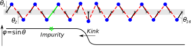
(a)

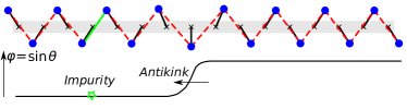
(b)

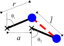
(c)

Figure 1: A kink (a) and an antikink (b) configuration in a topological chain (TC) model of rotors (blue) and springs (red dashed lines) in the presence of a single impurity (green solid lines) modeled as a spring with a different stiffness. For the kink profile, the springs in the chain are at their rest length, while for the antikink, they are stretched. A sketch of kink and antikink profiles in terms of the continuum field variable $u=\sin\theta$ (where $\theta$ is the rotor angle) is shown below each configuration. (c) A two-rotor system. The masses are the blue dots, the rigid rotors are the black lines, the pivots are the crosses, and the spring is the dashed red line. Here, $a$ is the lattice spacing, $r$ is the rotor length, $\bar{l}$ is the rest length of the springs and $\theta_{1,2}$ are the rotor angles with respect to the vertical.

In this paper we explore the physics of these finite-energy configurations. We compare the dynamics of the kink and antikink sectors in the topological rotor chain and study their interaction with a lattice impurity. We find that differences arising from the topological boundary term are apparent in all of these aspects. In Section II, we explain the discrete model and develop a fixed-point analysis of the kink motion using a cobweb plot. In Section III, we review the continuum theory and compare the predictions for the antikink with the discrete model. In Section IV, we study the eigenmodes of the chain around a single kink or antikink profile. We exploit the tangent stiffness matrix approach developed by Guest Guest (2006) to analyze prestressed structures. In Section V, we study the nonlinear transport properties. In a conventional continuum $\phi^{4}$ field theory, owing to translation invariance, both the kink and antikink propagate at uniform speed. However, lattice discreteness effects breaks this invariance and generates the so-called Peierls-Nabarro (PN) barrier Combs and Yip (1983); Braun and Kivshar (1998); Roy et al. (2007). For the topological rotor model, we find that only the antikink has a finite PN barrier whereas the kink always propagates freely. We explain this phenomenon as a consequence of the zero-energy cost associated with the kink profile. In Section VI, we investigate how kinks and antikinks interact with a spring constant impurity in the lattice. For the normal $\phi^{4}$ model, a phenomenological theory predicts alternating windows of initial kink (antikink) velocities that leads to reflection, trapping and transmission of the excitation Fraggis et al. (1989); Fei et al. (1992). By contrast, for the topological rotor model that we study, an impurity in the spring stiffnesses results in dramatically different scattering behaviors for the kink and antikink respectively. Fig. 2 summarizes all the possible scattering scenarios that we observe. Finally, in Section VII, we make a connection between linear mode analysis and nonlinear dynamics of kink motion in the context of spring length impurities. We conclude by listing some open questions related to our study.

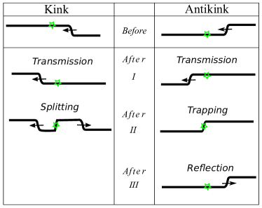
Figure 2: Illustrated are the possible scenarios for how the kink and antikink interact with a single impurity of spring stiffness. As indicated by the arrow, an initial kink or antikink approaches the impurity site (indicated by the green star) from the right. After scattering, the incident kink is either: (I) perfectly transmitted or (II) splits into a reflected kink, a transmitted kink and an antikink that gets trapped at the impurity site. The incident antikink is either: (I) perfectly transmitted, (II) trapped at the impurity site or (III) perfectly reflected.

II Discrete model and cobweb plot

The model we study consists of rotors of length $r$. The rotor pivots are placed on a 1D lattice with spacing $a$. The angles $\theta_{i}$ of the rotors are measured in an alternating fashion along the lattice, from the positive $y$-axis at odd-numbered sites and negative $y$-axis at even-numbered sites. The equilibrium angle is $\overline{\theta}$ for a uniform lattice configuration without a kink or antikink. The masses $M$ at the tips of the rotors are connected by harmonic springs with identical rest lengths $\overline{l}$ and spring constants $k$. The two-rotor unit cell of the topological chain is illustrated in Fig. 1c.

We now construct the chain with a kink under free boundary conditions. There are $n$ rotors and $n-1$ springs. If we assume that the springs are infinitely stiff ($k\rightarrow\infty$), the springs become $n-1$ constraints and the system only has a single independent degree of freedom. The angle of a single rotor determines all the others iteratively. This degree of freedom manifests itself as a mechanism which, as has been previously shown in Chen et al. (2014), can be approximately described by the domain wall solution in a modified $\phi^{4}$ theory . We call this mechanism a “kink” and discuss its continuum theory in the following sections.

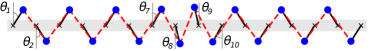
(a)

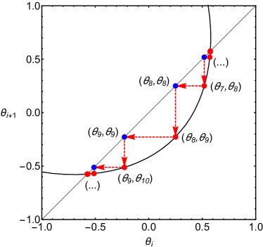
(b)

Figure 3: The configuration (a) and the corresponding cobweb plot (b) for the kink in a topological rotor chain with $r/a=0.8$, $|\overline{\theta}|=0.58$. The springs are at their rest lengths. In (b), the black curve is the constraint equation which ensures that the springs are unstretched, the gray diagonal line satisfies $\theta_{i+1}=\theta_{i}$, the blue point $(\theta_{i},\theta_{i})$ represents rotor $i$, the red point $(\theta_{i},\theta_{i+1})$ represents the spring connecting rotors $i$ and $i+1$, and the red dashed lines with arrows indicates the iterative process that generates the kink profile. The iteration steps from $\theta_{7}$ to $\theta_{10}$ are shown.

We use a cobweb plot to display the kink in Fig. 3. This is a tool for visualizing the process of iteratively solving the nonlinear constraint equations Eqn. (3) cell by cell. We construct the cobweb plot by drawing (1) a diagonal line $\theta_{i}=\theta_{i+1}$ and (2) a curve of the implicit function given by the nonlinear constraint equation that ensures the springs are not stretched,

$$(a+r\sin\theta_{i}-r\sin\theta_{i+1})^{2}+(r\cos\theta_{i}+r\cos\theta_{i+1})^{2}=\overline{l}^{2}.$$ (3)

(An explicit relation between neighbouring rotor angles is derived analytically with complex notation in Appendix A.)

The iteration steps are as follows:

1. Given the angle $\theta_{1}$ of the first rotor at the left end, find the point on the function curve with coordinates $(\theta_{1},\theta_{2})$.

2. Draw a horizontal line from $(\theta_{1},\theta_{2})$ to the diagonal line. This gives the point $(\theta_{2},\theta_{2})$.

3. Draw a vertical line from $(\theta_{2},\theta_{2})$ to the function curve. This gives the point $(\theta_{2},\theta_{3})$.

4. Repeat step 2 and 3 until the point $(\theta_{n-1},\theta_{n})$ is found.

In Fig. 3b, we illustrate steps 2 and 3 from $\theta_{7}$ to $\theta_{10}$, which are near the kink center. The blue point with coordinates $(\theta_{i},\theta_{i})$ stands for the $i$th rotor of angle $\theta_{i}$. The red point with coordinates $(\theta_{i},\theta_{i+1})$ represents the state of the spring that connects the rotors of $\theta_{i}$ and $\theta_{i+1}$.

Note that in Fig. 3b, the diagonal line and the function curve intersect at two points. They are the fixed points of iteration. If all the red points $(\theta_{i},\theta_{i+1})$ stay at one fixed point, the plot represents a uniform lattice. The iteration step proceeds from the leftmost rotor of the chain to the rightmost. We see that the flow proceeds outwards from one fixed point and then inwards towards the other fixed point.

The cobweb plot may be used to graphically derive the decay lengths of zero energy deformations, as they approach their uniform limits. As mentioned above, a fixed point corresponds to an intersection between the line $\theta_{i}=\theta_{i+1}$ and the function curve. Note that the behavior of $\theta_{i}$ as it approaches a fixed point resembles a ”self-similar” zigzag motion between $\theta_{i}=\theta_{i+1}$ and the tangent line of the function curve. This motivates linearizing the function curve around the fixed point as follows:

$$\theta_{i+1}-\overline{\theta}=F^{\prime}(\overline{\theta})(\theta_{i}-\overline{\theta}),$$ (4)

where $\overline{\theta}$, the equilibrium angle, is also just the value of the fixed-point angle and $F^{\prime}(\overline{\theta})$ is the slope of the function curve at that point (which could be computed explicitly in terms of $r,a,\overline{l}$). This equation yields that $\theta_{i}-\overline{\theta}\propto\exp(\log F^{\prime}(\overline{\theta})i)$, or that the decay length is $|1/\log F^{\prime}(\overline{\theta})|$ (the sign of $\log F^{\prime}$ tells us whether the fixed point is attracting or repelling). This result recovers the penetration depth of the boundary modes computed in Ref. Chen et al. (2014) using band theory.

In the cobweb plot, the static kink appears as a sequence of points on the function curve interpolating between a repelling and attracting fixed point. The dynamics of the kink in the cobweb plot is therefore the flow of a cascade of points between a pair of fixed points (Movie S1). While the kink propagates, the points in the middle, such as $(\theta_{7},\theta_{8})$, $(\theta_{8},\theta_{9})$ and $(\theta_{9},\theta_{10})$, corresponding to the kink center, move more than those points close to the fixed points, corresponding to the spatially localized nature of the kinetic energy.

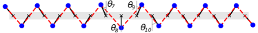
(a)

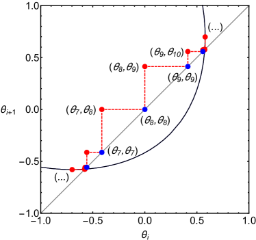
(b)

Figure 4: The configuration (a) and the corresponding cobweb plot (b) for an antikink profile in the topological rotor chain with $r/a=0.8$, $|\overline{\theta}|=0.58$, where we see that the springs are stretched. In (b) the same graphic notation as in Fig. 3 is used except that we have not used an iterative process for constructing the antikink profile, rather, depicted is only a visualization of the configuration of the rotor chain. The red points are obtained by first reflecting the red points in Fig. 3b across the diagonal line, and then relaxing the springs using dissipative Newtonian dynamics. Note that the two rotors at the edges need to be collinear with the springs to ensure force balance. This results in the angles overshooting at the fixed points.

Generating an antikink requires a few more steps, as it stretches springs, and thus does not satisfy a constraint function that we could iteratively solve. However, the continuum theory suggests that kinks and antikinks both have the same functional profiles with only their signs reversed (see Section III). As a result, we use the same iterative procedure as that for the kink, and then simply swap the appearances of $\theta_{i}$ and $\theta_{i+1}$ in Eqn. (3) to obtain an approximation for the antikink profile. This method is equivalent to reflecting the red points in Fig. 3b across the diagonal line. The antikink constructed this way is not an equilibrium configuration and has unbalanced stresses in the springs. This is because generically, the profiles of the kink and antikink are not the same in a discrete topological rotor chain. We next relax the springs using dissipative Newtonian dynamics to remove the unbalanced stresses and obtain a stable profile, which we show in the cobweb plot in Fig. 4. In that figure, the spring connections (red dots) around the core of the antikink profile (rotors 8 and 9) do not fall on the curve which corresponds to unstretched springs. This implies large spring deformations which we show explicitly in Fig. 5b. The amount by which the springs are stretched is symmetrical around the 8th spring, which is in accordance with the fact that a stable antikink has balanced forces on each rotor. Note that we have fixed the boundary conditions to ensure that the antikink is in mechanical equilibrium, which is not generically true. As discussed later in Section V, this has important consequences for the PN barrier.

(a)

(b)

Figure 5: (a) The $\theta$ profile (rotor angles) for the antikink profile in Fig. 4a and the corresponding continuum prediction from Eqn. (13). Note that the two rotors at the edges need to be collinear with the springs to ensure force balance and this results in the rotor angles overshooting the equilibrium value $\overline{\theta}=\pm 0.58$. (b) The amount of spring stretching for the antikink profile.

III Continuum theory

In this section, we review the continuum approximation to the kink and antikink profiles Chen et al. (2014) and compare these with the discrete model developed in the previous section. The discrete Lagrangian for the topological rotor chain (see also Fig. 3a) with free boundary conditions is

$$L=\sum_{i=1}^{n}\frac{1}{2}Mr^{2}\bigg{(}\frac{\mathrm{d}\theta_{i}}{\mathrm{d}t}\bigg{)}^{2}-\sum_{i=1}^{n-1}\frac{1}{2}k(l_{i,i+1}-\overline{l})^{2}.$$ (5)

Here, $n$ is the total number of rotors, $M$ is the mass at the tip of a rotor, $r$ is the rotor length, $\theta_{i}$ is the angle that rotor $i$ makes with the vertical (measured alternately as shown in Fig. 3a), $k$ is the spring constant, $\overline{l}$ is the rest length of the spring and $l_{i,i+1}$ is the instantaneous length of the spring that connects rotor $i$ to rotor $i+1$. From geometry

$$\begin{split}l_{i,i+1}^{2}&=a^{2}+2ar(\sin\theta_{i+1}-\sin\theta_{i})+2r^{2}+\\ &~{}~{}~{}~{}2r^{2}\cos(\theta_{i}+\theta_{i+1}).\end{split}$$ (6)

which in the uniform limit $\theta_{i}=\theta_{i+1}=\bar{\theta}$ gives the rest length of the spring $\overline{l}^{2}=a^{2}+4r^{2}\cos^{2}\overline{\theta}$.

We make the working assumption that deformations do not stretch the springs significantly and hence we can neglect (or add) terms higher than quadratic order in $l_{i,i+1}-\overline{l}$ for all $i$. This is a reasonable approximation for the system configuration with a kink profile but is not well-justified for an antikink profile. However, in the limit that $\overline{\theta}\ll 1$, we find this to be a good approximation for both kinks and antikinks. Within this limit, we therefore express the potential energy term in Eqn. (5) as

$$\begin{split}\frac{1}{2}k(l_{i,i+1}-\overline{l})^{2}&\approx\frac{k}{8\overline{l}^{2}}\bigg{(}l^{2}_{i,i+1}-\overline{l}^{2}\bigg{)}^{2}.\end{split}$$ (7)

Substituting the expression for $\bar{l}$ and Eqn. (6) into Eqn. (7), we express the potential energy as

$$\begin{split}V_{i,i+1}&=\frac{kr^{4}}{2\overline{l}^{2}}\bigg{(}\frac{a}{r}(\sin\theta_{i+1}-\sin\theta_{i})\\ &~{}~{}~{}~{}-\cos 2\overline{\theta}+\cos(\theta_{i}+\theta_{i+1})\bigg{)}^{2}.\end{split}$$ (8)

Now we take the continuum limit of the potential. First we define a continuum field for the rotor angles $\theta(x)$, where the spatial variable $x=ia+\frac{a}{2}$ is located symmetrically between two rotors in the unit cell. To leading order, $\theta_{i}\rightarrow\theta(x)-(a/2)(\mathrm{d}\theta/\mathrm{d}x)$ and $\theta_{i+1}\rightarrow\theta(x)+(a/2)(\mathrm{d}\theta/\mathrm{d}x)$. Eqn. (8) can then be expressed as

$$\begin{split}aV[\theta]&=\frac{2k}{\overline{l}^{2}}\left(\frac{a^{2}}{2}\frac{\mathrm{d}u}{\mathrm{d}x}+\overline{u}^{2}-u^{2}\right)^{2},\end{split}$$ (9)

where we have defined the projection of the rotor position on the $x-$axis as a new field variable $u(x)\equiv r\sin\theta(x)$ and $\overline{u}\equiv r\sin\overline{\theta}$.

The kinetic energy density term in Eqn. (5) then assumes the form

$$\begin{split}aT[\dot{\theta}]&=\frac{1}{2}\frac{Mr^{2}}{r^{2}-u^{2}}\bigg{(}\frac{\mathrm{d}u}{\mathrm{d}t}\bigg{)}^{2}.\end{split}$$ (10)

Next we approximate the Lagrangian Eqn. (5) as

$$\begin{split}L&\approx\int\mathrm{d}x\bigg{\{}\frac{M}{2a}\Big{(}\frac{\partial u}{\partial t}\Big{)}^{2}-\frac{ka^{3}}{2\overline{l}^{2}}\bigg{(}\frac{\partial u}{\partial x}\bigg{)}^{2}\\ &~{}~{}~{}~{}~{}~{}~{}~{}~{}~{}~{}~{}~{}~{}~{}-\frac{2k}{a\overline{l}^{2}}(\overline{u}^{2}-u^{2})^{2}-\frac{ka}{\overline{l}^{2}}\frac{\partial u}{\partial x}(\overline{u}^{2}-u^{2})\bigg{\}}.\end{split}$$ (11)

where we have taken the leading order of the Taylor series expansion of the nonlinear kinetic term (in the variable $u^{2}/r^{2}$), which is valid in the limit when $u\ll r$ or equivalently $\sin\theta\ll 1$.

The first three terms in Eqn. (11) constitute the normal $\phi^{4}$ theory. The last term linear in $\partial u/\partial x$, is an additional topological boundary term. Being a total derivative, it does not enter the Euler-Lagrange equation of motion and we obtain the usual nonlinear Klein-Gordon equation

$$\begin{split}\frac{M}{a}\frac{\partial^{2}u}{\partial t^{2}}-\frac{ka^{3}}{\overline{l}^{2}}\frac{\partial^{2}u}{\partial x^{2}}-\frac{8k}{a\overline{l}^{2}}\overline{u}^{2}u+\frac{8k}{a\overline{l}^{2}}u^{3}=0,\end{split}$$ (12)

whose kink and antikink solutions are given by

$$\begin{split}u_{0}=\pm\overline{u}\tanh\Bigg{[}\frac{x-x_{0}-vt}{(a^{2}/2\overline{u})\sqrt{1-v^{2}/c^{2}}}\Bigg{]},\end{split}$$ (13)

where the $\pm$ denotes an (+)antikink and (-)kink respectively. Here, $v$ is the (anti)kink speed of propagation and $c=(a^{2}/\overline{l}\sqrt{k/M})$ is the speed of sound in the medium. See Fig. 5a for a comparison with the discrete profile.

Note how the additional boundary term makes the potential energy density $V[\theta]$ a perfect square, see Eqn. (9). For the kink configuration, $V[\theta]$ therefore vanishes as is the case in the discrete topological chain. For the antikink however, $V[\theta]$ is nonzero and is in fact twice of what we would expect in the normal $\phi^{4}$ theory (where both the kink and antikink configurations have the same energy). This is an agreement with our discussion on the discrete model in Section II.

Upon substituting the static ($v=0$) antikink profile from Eqn. (13) into Eqn. (11) and completing the integral, we obtain the potential energy of the topological rotor chain with an antikink profile

$$\begin{split}V_{antikink}/(ka^{2})=\frac{16}{3}\frac{(r/a)^{3}\sin^{3}\overline{\theta}}{1+4(r/a)^{2}\cos^{2}\overline{\theta}}.\end{split}$$ (14)

In Fig. 6, we compare this expression with the predictions from the discrete model. We see that the continuum theory agrees reasonably well with the discrete model as long as $\overline{\theta}$ is less than approximately 0.6, below which, the width of the antikink is larger than the lattice spacing and therefore, a continuum approximation well justified.

Figure 6: The normalized potential energy plotted against the equilibrium angle $\overline{\theta}$, for a static antikink configuration in a topological rotor chain with with $r/a=0.8$. The discrete model has 60 rotors. Note that the wobbler transition Chen et al. (2014) is around $\overline{\theta}=\sin^{-1}\left(\frac{a}{2r}\right)=0.67$, which is close to where the continuum theory starts to significantly deviate from the discrete model.

IV Linear mode analysis: tangent stiffness matrix approach

We now study small oscillations around the kink and antikink configurations, first in the continuum limit, and next in the discrete model by developing the tangent stiffness matrix approach. In the continuum limit, we make the ansatz $u=u_{0}+\delta u$ and substitute into Eqn. (12) retaining only terms linear in $\delta u$:

$$\begin{split}\frac{M}{a}\frac{\partial^{2}\delta u}{\partial t^{2}}-\frac{ka^{3}}{\overline{l}^{2}}\frac{\partial^{2}\delta u}{\partial x^{2}}-\frac{8k}{a\overline{l}^{2}}(\overline{u}^{2}-3u_{0}^{2})\delta u=0\end{split}$$ (15)

If we Fourier transform Eqn. (15) with respect to time, we obtain a Schödinger-like equation with a solvable potential Campbell et al. (1983); Makhankov (1990). This yields one continuous spectral band as well as two discrete modes – one translation mode for the (anti)kink and one shape mode, which corresponds to small deformations of the shape of the (anti)kink localized around the center of their profile. For the topological rotor chain, the frequencies of the two discrete modes are:

$$\begin{split}\omega_{t}&=0,~{}~{}\textrm{for the translation mode}\\ \end{split}$$ (16)

$$\begin{split}\omega_{s}&=(r/a)\sqrt{12k/M}\sin\overline{\theta}/\sqrt{1+4(r/a)^{2}\cos^{2}\overline{\theta}},\\ &~{}~{}~{}~{}~{}~{}~{}~{}~{}~{}~{}~{}~{}~{}~{}~{}~{}~{}~{}\textrm{for the shape mode}.\end{split}$$ (17)

In Fig. 7a and 7c, the kink and antikink are located in the middle of the chain. The mode arrows (in green) that all point in the same direction, correspond to a translation mode. In Fig. 7b and 7d, the arrows on either side of the (anti)kink, point in opposite directions and these correspond to shape deformations of the (anti)kink.

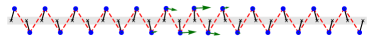
(a)

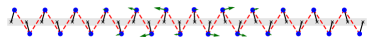
(b)

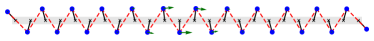
(c)

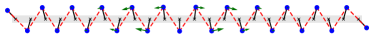
(d)

Figure 7: The configurations of (a) the kink translation mode, (b) the kink shape mode, (c) the antikink translation mode and (d) the antikink shape mode. The green arrows depict the mode component of each rotor.

In Appendix B, we follow the approach proposed by Guest Guest (2006) to derive the tangent stiffness matrix $\mathbf{K}$ for prestressed mechanical structures. With $\mathbf{K}$ we numerically obtain the frequencies of localized modes for the discrete chain model and compare them with the predictions of the continuum theory (Eqn. (16) and Eqn. (17)) in Fig. 8. We find that the translation mode $\omega_{t}$ for the kink indeed vanishes (within machine-precision in our numerics) for all values of $\overline{\theta}$ and is thus absent in the range of the log-log plot shown in Fig. 8a). However, as seen in Fig. 8b, the translation mode (open circles) for the antikink is nonzero.

For the shape mode $\omega_{s}$ (filled circles), we find the numerical results for both the kink and antikink to be in good agreement with the continuum theory at small $\overline{\theta}$. Note that in Fig. 8b, although the antikink has a finite nonzero $\omega_{t}$, the value is still significantly smaller than $\omega_{s}$.

(a)

(b)

Figure 8: The frequencies $\omega$ of localized mode(s) for (a) the kink and (b) the antikink as a function of $\overline{\theta}$ for a rotor chain with $r/a=0.8$. The data points are numerically obtained from the tangent stiffness matrix approach, filled circles correspond to the shape mode ($\omega_{s}$), while open circles correspond to the translation mode ($\omega_{t}$) . The curves are from the continuum theory. The frequencies for the kink translation mode for all $\bar{\theta}$ and the frequencies for the antikink translation mode for $\overline{\theta}<0.1$ are effectively zero at machine precision and thus, not visible in the figure.

V Kink/antikink propagation in ordered lattices

In the previous section, we have seen that for the discrete topological chain, the energy of the translation mode for the kink is zero, whereas that for the antikink is non-zero. Note that the standard discretization of a $\phi^{4}$ field theory leads to a non-zero translation mode for both the kink and antikink  Roy et al. (2007). Thus, the kink here differs qualitatively from the antikink in that it has a zero mode even when we consider the discrete model. We next numerically simulate the propagation of a kink and antikink along the discrete chain and see how this difference manifests in their dynamics.

We numerically integrate Newtons equation of motion for the rotors using molecular dynamics simulations. (The simulation settings are described in Appendix C.) A stable chain configuration with a single kink or antikink is used as the initial configuration (see Figs. 7a- 7c for the initial conditions used). An excitation is set in motion with a velocity along the direction of the translation mode, but with variable amplitudes.

In Fig. 9, we plot the kinetic energy (K.E.) of the chain as a function of time for a set of parameters, for a kink excitation (solid curve) and an antikink excitation (dashed curve). The K.E. of the kink remains nearly constant for all times with some small fluctuations (as the springs have to slightly deform to transport energy by simultaneously minimize the potential and kinetic energy). However in comparison, the K.E. of the antikink for the same set of initial parameters changes significantly as it propagates down the chain. The key point is that the kink and antikink do not propagate in the same way.

The asymmetry between a static kink and antikink configuration was discussed in Chen et al. (2014). Further, we also know from Eqn. (11) (and the ensuing discussion) that in the continuum limit, the topological rotor chain is approximately described by a $\phi^{4}$ theory with an additional topological boundary term which ensures that the potential energy of the kink is zero while that for the antikink is nonzero (see Ref. Vitelli et al. (2014) for an interpretation of this fact in terms of supersymmetry breaking). However, the additional boundary term does not affect the continuum equation of motion and thus, both the kink and antikink should have translational invariance in this limit and their dynamics should not have differed.

The reason for this asymmetrical behavior can be understood only if we examine the discrete model. The system with free boundary conditions has $n$ rotors and $n-1$ springs, and the static kink does not require any of the springs to be stretched. We can therefore interpret the springs as constraints. Thus, the discrete kink’s equilibrium manifold is a continuous curve embedded in the $n$-dimensional configuration space of the rotor angles $\theta_{i}$ and the kink can be positioned stably anywhere along the chain. By contrast, an antikink requires the springs to be stretched. Forces on each of the rotors have to be balanced for the system to be in mechanical equilibrium. So the possible equilibrium configurations have to be symmetrical locally around the center of the antikink, as shown in Fig. 10. As a result, the equilibrium manifold for an antikink is not a continuous curve but rather, consists of a set of discrete points. These correspond to either saddle points or minima in the potential landscape. Any locally asymmetrical configuration is therefore not stable and will slide towards a minima.

The saddle points and their nearest minima can be connected by an “adiabatic trajectory” Braun and Kivshar (1998), which is a curve of steepest descent. The concept of an adiabatic trajectory is useful in two ways. First, it describes the slow motion of the antikink through the chain. The position of the antikink center can be defined by a coordinate along such a trajectory. Secondly, it helps to rigorously define the so-called Peierls-Nabarro (PN) potential Combs and Yip (1983); Braun and Kivshar (1998); Roy et al. (2007), which is the effective periodic potential that the antikink feels as it moves along the adiabatic trajectory. A saddle point in the full potential energy landscape corresponds to a maximum along the adiabatic trajectory (while a minimum is still a minimum). Note that although the antikink’s K.E. fluctuations in Fig. 9 do not strictly equal its PN potential barrier, the former reveals the existence of the latter.

Figure 9: Time evolution of the kinetic energy for a kink (Fig. 7a) and an antikink (Fig. 7c) in a topological rotor chain with non-dimensional parameters $M=1$, $k=10000$, $r/a=0.8$, $\overline{\theta}=0.58$. The magnitude of initial velocity in both cases is $v_{0}=2.4$. The units of energy and velocity are determined by the aforementioned physical parameters. The kink propagation only results in small oscillation of the K.E. whereas we see significant fluctuations during the propagation of an antikink. These can be traced to the Peierls-Nabarro potential as shown in Fig. 10

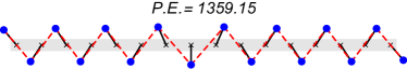
(a)

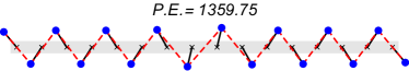
(b)

Figure 10: Two equilibrium configurations in the potential energy landscape of a static antikink: (a) a minimum and (b) a saddle point, respectively. The topological chain has the same configuration parameters as in Fig. 9.

In Appendix D, we derive the PN potential barrier from the continuum theory

$$\begin{split}V_{PNB}&=\frac{4\pi^{2}\big{(}\pi^{2}+(a/w)^{2}\big{)}}{3\big{(}1+4(r/a)^{2}-(a/w)^{2}\big{)}\sinh(\pi^{2}w/a)}\\ &\propto e^{-\pi^{2}w/a}~{}~{}~{}~{}~{}~{}~{}~{}~{}~{}~{}~{}\textrm{for large $w/a$.}\end{split}$$ (18)

This shows that the PN barrier decays exponentially as the width $w$ of the antikink increases.

Figure 11: The dependence of the normalized PN barrier ($V_{PNB}/ka^{2}$) on the normalized antikink width ($w/a$), for both the discrete model (black circles) and the continuum theory (solid line). The slope of the dashed line (fit to simulation) is $-10.6$, in reasonable agreement with the predictions from the continuum theory in Eqn. (18), which gives a slope $-\pi^{2}\approx-9.9$.

We next compare the theoretical results with numerical simulations. We obtain the exact PN barrier by computing the difference in potential energy between the two types of equilibrium points: a minima and a saddle point, see Fig. 10, where for a given set of parameters, we find the barrier height to be $1359.75-1359.15=0.60$, consistent with the magnitude of the K.E. fluctuations shown in Fig. 9 for the same set of parameters. By repeating this calculation for systems with various antikink widths $w$, we obtain the dependence of the normalized PN barrier $V_{PNB}/(ka^{2})$ on $w/a$, which we show in Fig. 11. We compare these with the predictions from the continuum theory, given by Eqn. (18). The numerical results (filled circles) obtained from the discrete lattice and the theoretical predictions (continuous curve) follow a similar trend, but differ by at least one order of magnitude. This can be explained by the fact that the discreteness of the lattice is ignored in the theory when we take the continuum limit in going from Eqn. (8) to Eqn. (9). See Combs and Yip (1983) for a thorough discussion of the effect of lattice discreteness on the single-kink dynamics in a $\phi^{4}$ model.

Figure 12: The finite-size effect on $V_{PNB}$. $\Delta V_{PNB}$ is defined as $V_{PNB}(L)-V_{PNB}(L=60)$. The configuration parameters are $r/a=0.8$ and $\overline{\theta}=0.40$.

Further, we also investigate finite-size corrections to the PN barrier, or more precisely, the difference between $V_{PNB}$ for a system with a small finite size and that for a system with a sufficiently larger size (60 rotors). We find that finite size effects decay quickly as an exponential function with increasing system size for a topological rotor chain with a central antikink (see Fig. 12). This is because an antikink configuration is a localized object. The components of its displacement, its translation mode, as well as its shape mode, decay exponentially away from its center and therefore, so does the effect of any boundaries.

To summarize, for the topological rotor chain that we study, the PN barrier for a kink vanishes and that for an antikink is finite. This, not only affects how their respective kinetic energies fluctuate over a lattice spacing, but also affects their dynamics over long distances. It is well known that $\phi^{4}$ kinks and antikinks are non-integrable solutions  Makhankov (1990). Although the kinks and antikinks are “topologically” robust objects, they still tend to dissipate energy into phonons and into shape fluctuations as they propagate. Once an antikink has lost too much kinetic energy to be able to overcome the PN barrier, it gets trapped in a PN potential minimum, as shown in Fig. 13. On the other hand, for the topological rotor chain that we study, the kink never gets trapped, since its PN barrier vanishes.

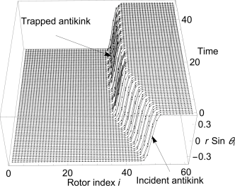
Figure 13: Perspective view of a moving antikink trapped in its Peierls-Nabarro barrier around $\textrm{Time}=20$ near Rotor #35. The topological rotor chain has the same configuration parameters as in Fig. 9 and the initial antikink velocity is $v_{0}=1.1$ in non-dimensional units.

VI Effect of spring stiffness impurities

We next numerically explore whether the kink-antikink asymmetry also manifests in the way these excitations interact with a single lattice impurity, a natural starting point to study their propagation in disordered lattices. For the conventional $\phi^{4}$ models, previous studies on kink-impurity interactions (in both discrete models Fraggis et al. (1989) and continuum field models Fei et al. (1992)) have shown that scattering can result in transmission, trapping or reflection of kinks, depending on the type of the impurity, the attraction/repulsion strength of the impurity and the kink’s initial velocity. Although similar scattering also occurs in the topological rotor chain model, we also find other novel phenomena, for instance, the kink can split into two kinks and one antikink. Moreover as we will see, kinks and antikinks no longer scatter in the same way – a feature which underscores the kink-antikink asymmetry in our topological rotor chain. In this work, we study impurities in properties of the springs, which yield a richer set of effects on the response than mass impurities.

In this section, we model an impurity by changing the spring stiffness constant at a single site (Fig. 1a). We study a topological chain with lattice spacing $a=1$ and rotor length $r/a=0.8$ and with equillibirum angle $\overline{\theta}=0.28$. We perform Newtonian dynamics simulation on a system with 60 rotors using free boundary conditions, and for a range of impurity spring stiffness constant $k_{i}$ and kink/antikink initial velocity $v_{0}$. See Fig. 2 for a table of the possible scattering scenarios that we observe.

Consider first the kink-impurity interaction. For most $k_{i}$ and $v_{0}$, the kink simply passes through the impurity and may excite an impurity mode, which can be seen in the form of small fluctuations in the middle of the chain as shown in Fig. 14a. When the impurity spring is sufficiently soft, the incident kink splits into three: a transmitted kink, an antikink that is trapped at the impurity and a reflected kink. This is shown in Fig. 14b.

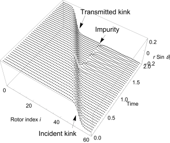
(a)

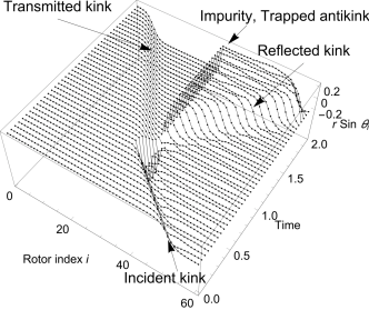
(b)

Figure 14: A kink interacts with an impurity (different spring stiffness) and is either (a)  transmitted, shown here for $v_{0}=4.0$ and $k_{i}/k=0.10$ or (b) splits into a transmitted kink, a reflected kink and an antikink trapped at the impurity, shown here for $v_{0}=9.6$ and $k_{i}/k=0.01$. The non-dimensional parameters are $M=1,k=10000,r/a=0.8,\bar{\theta}=0.28$.

Antikink scattering results in an ever richer set of behaviors. Recall that the springs near the location of an antikink are always stretched significantly, see Fig. 5b. For $k_{i}/k$ near 1, the antikink gets transmitted with energy dissipation and thus slows down (Fig. 15a). Softening the impurity spring stiffness creates an attractive potential well for the antikink. The antikink may then release a part of its potential energy and get trapped at such an impurity site (Fig. 15b). If the impurity spring is made even softer, such that an antikink can no longer transfer its kinetic energy forward or dissipate it sufficiently quickly to be trapped, the incident antikink is completely reflected (Fig. 15c). For similar reasons, a stiffer impurity acts like a repulsive potential well that can reflect slow moving antikinks.

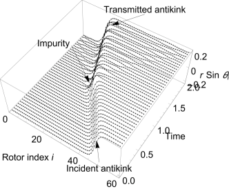
(a)

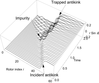
(b)

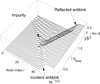
(c)

Figure 15: An antikink interacts with an impurity and is either (a) transmitted, shown here for $v_{0}=4.0$ and $k_{i}/k=0.80$, (b) trapped, shown here for $v_{0}=4.0$ and $k_{i}/k=0.70$ or (c) reflected, shown here for $v_{0}=4.8$ and $k_{i}/k=0.20$. The system parameters are the same as Fig. 14.

These numerical results are summarized in the phase diagrams in the space of $k_{i}$ and $v_{0}$ in Fig. 16. First, note that a kink (Fig. 16a) behaves quite differently from an antikink (Fig. 16b). For instance, a kink is never completely trapped or reflected by an impurity. The reason is that it has zero intrinsic potential energy and thus, no potential energy to lose during a scattering event. As a collective object, the kink experiences a flat potential landscape along the chain. It will always go through the impurity, unless $k_{i}$ is so soft or $v_{0}$ is so large that the initial kinetic energy of the kink is sufficient to stretch the impurity spring to form a pinned antikink. That is when scattering results in the kink being split. This also explains the positive slope of the boundary line between these two regimes. (The topological constraints of the field require that the number of kinks minus the number of antikinks remains constant Manton and Sutcliffe (2004), which is one for our boundary conditions.)

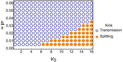
(a)

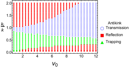
(b)

Figure 16: The phase diagram of the scattering behavior in the parameter space of normalized spring constant of impurity $k_{i}/k$ and kink initial velocity $v_{0}$ for (a) the kink and (b) the antikink. The system parameters are the same as Fig. 14. The lower limit of $v_{0}$ for the antikink is around 0.7, below which even the PN barrier in a perfect chain will capture the antikink.

For an antikink, the scattering phase diagram has more regimes (Fig. 16b). The positive slope of the boundary curve at higher $k_{i}$ between the upper reflection regime (square) and the transmission regime (circle) comes from the fact that the higher the barrier is, the faster the antikink needs to be, to get transmitted. The negative slope of the boundary between the transmission regime (circle) and the trapping regime (triangle), suggests that a softer impurity spring causes the antikink to dissipate more energy. The antikink then needs a sufficiently high initial velocity to avoid being trapped at such an impurity site. The positive slope of the curve between the trapped regime (triangle) and the lower reflection regime (square) suggests that if the impurity spring is so soft such that it can no longer transform the kinetic energy into other forms or channelize the kinetic energy to the other side of the impurity sufficiently “quickly”, an antikink incident with sufficiently high energy will then be completely reflected. (In simulations we find that the maximum initial velocity with which we can launch an antikink is around $v_{0}=12$. Above this, the antikink itself becomes unstable and tends to quickly disintegrate.)

For the topological rotor chain, the antikink scattering behaviour is therefore very similar to the ones reported for kinks and antikinks in previous studies on the $\phi^{4}$ model Fei et al. (1992); Fraggis et al. (1989). In addition, for normal $\phi^{4}$ kinks and antikinks, one also observes resonance windows which are alternating regimes of the excitation being reflected or trapped, along the axis of initial velocities for a given impurity strength. These have not been observed during our simulations of the discrete topological chain. Instead, we only observe a small range of alternating regimes where the antikink is transmitted or trapped, around $k_{i}/k=0.75$ and $v_{0}=3.6$ in Fig. 16b. We leave a detailed characterization of the resonance energy exchange between these modes for future studies.

VII Effect of bond length impurities

In section IV we perform linear mode analysis of the topological chain, and in section VI we study the nonlinear motion of (anti)kinks with impurities. Here in this section we will show in a qualitative way that there is a connection between these two aspects. For convenience, we investigate another type of impurity: the spring length.

VII.1 Linear mode analysis

We start with a qualitative observation of the linear vibrational modes. For a perfect topological rotor chain with free boundary conditions, there exists only one zero mode – the translation mode of the kink. This is what the Maxwell-Calladine counting predicts Maxwell (1864); Calladine (1978): the chain has $n$ rotors as degrees of freedom and $n-1$ springs as constraints, and the former quantity minus the latter equals the number of zero modes minus the number of states of self stress. (In a perfect chain there is no states of self stress.) This counting does not depend on the geometrical parameters of the chain components.

Now we increase one geometrical parameter, namely the length of the middle spring $l_{0}$, so that it is an impurity in the system (Fig. 17). As long as no state of self stress is created, there remains only one zero mode. However, as $l_{0}$ approaches a critical value $l_{critical}$, several qualitative changes take place: (1) The profile of the chain varies significantly. There are two kinks, one on each side of the impurity spring. (2) Eigenmode analysis shows that the amplitude of the zero mode has two prominent parts that are spatially separated, each of which is localized around a kink as an individual translation mode. Both parts of the zero mode point towards the same direction. (3) An additional soft vibrational mode appears, whose amplitude also has two separated parts just like the zero mode. But the directions of these two parts are opposite to each other. This soft mode has a frequency close to zero, much lower than that of kink shape modes. (4) A soft tensional mode dual to the soft vibrational mode emerges, being localized around the impurity spring. (A tensional mode is a vector whose components are the infinitesimal spring tensions caused by the infinitesimal motion of the dual vibrational mode. The duality comes from the fact that the tensional mode is an eigenfunction of the supersymmetrical “partner” of the dynamical matrix, while the vibrational mode is an eigenfunction of just the dynamical matrix. See Kane and Lubensky (2013); Vitelli et al. (2014); Lubensky et al. (2015) for more details.)

These changes do not contradict the Maxwell-Calladine counting: only one vibrational mode has strictly zero frequency, unless $l_{0}$ actually reaches $l_{critical}$. In that case, the frequencies of both the soft vibrational mode and the soft tensional mode go to zero. By definition the tensional mode becomes a state of self stress. Then the Maxwell-Calladine counting still holds as there are now two zero modes and one state of self stress.

The above analysis only considers infinitesimal oscillations around zero-energy equilibrium points. In the next section, we study qualitatively the nonlinear motion of kinks with finite energy, providing a perspective complementary to the linear analysis.

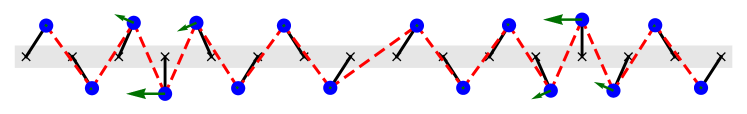
(a)

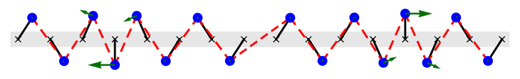
(b)

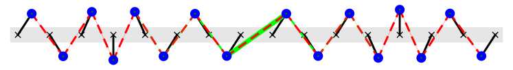
(c)

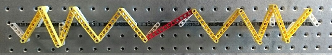
(d)

Figure 17: The zero vibrational mode (a), the soft vibrational mode (b), and the soft tensional mode (c) of a topological chain with a longer spring in the middle as an impurity. The configuration parameters are $\overline{\theta}=0.58$, $r/a=0.8$, $\overline{l}/a=1.68$, $l_{0}/a=2.30$ and $l_{critical}/a=2.31$. The soft mode frequency is $7.7\times 10^{-9}$ in the unit of $(r/a)\sqrt{k/M}$, which means the mode is much “softer” than the kink shape mode whose frequency is of the order $10^{-2}$. In (a) and (b), the arrows indicate the mode amplitude of the displacement of each rotor. In (c), the thickness of the green bars indicates the tensional mode amplitude on each spring. All the springs, both normal ones and the impurity, have the same stiffness. (d) shows a LEGO demonstration.

VII.2 Nonlinear dynamics: linkage limit

VII.2.1 Setup: Hamiltonian

To simplify the problem, we consider the linkage limit, where all the springs in a perfect chain are non-deformable rigid bars so that they are holonomic constraints.There is only one degree of freedom which is the translational motion of the kink. We choose the kink position $x$ as a collective variable to describe this degree of freedom.

Then we introduce the impurity by replacing the middle rigid bar with a longer spring that is “soft” (i.e. with a finite spring constant) (Fig. 18a). A soft spring does not strictly constrain the angles of the two rotors it connects but rather gives a potential energy to deviations from its preferred length. The chain then has one fewer constraint, which in turn means that it has two degrees of freedom. We regard the whole chain as two linkage sub-chains, then the two degrees of freedom are shared by the two kinks of the sub-chains, which we call Kink 1 and Kink 2 with position $x_{1}$ and $x_{2}$ respectively. The coordinate system for the discrete chain model is illustrated in Fig. 18a, and its precise definition is contained in Appendix E. We see that by taking the linkage limit, the number of degrees of freedom is reduced from the number of rotors (16 for the chain in Fig. 18a) to the number of kinks (2 for two kinks).

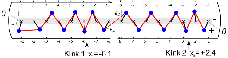
(a)

(b)

Figure 18: (a) Illustration of the coordinate system of a topological rotor linkage chain with $\overline{\theta}=0.58$, $r/a=0.8$, $\overline{l}/a=1.68$ and $l_{critical}/a=2.31$. The linkage bars are the solid lines and the impurity spring is the dashed line. In (b), the upper panels show the potential functions in 2D configuration space for various $l_{0}$. One corner of the function is trimmed for visualization. The red curve corresponds to the potential for Kink 1 in the one d.o.f. case where Kink 2 is fixed at $x_{2}=0$. The lower panels show the phase portraits of Kink 1.

Now we derive the Hamiltonian. Note that the potential energy only comes from the deformation of the impurity spring, which in turn just depends upon the angles of the head rotors $\tilde{\theta}_{i}$. Since $x_{i}$ is the degree of freedom, it determines the state of the sub-chain $i$, including $\tilde{\theta}_{i}$. Thus from the continuum theory (Eq. 13 where $u=r\sin\theta$), we obtain $\tilde{\theta}_{i}(x_{i})$:

$$\sin\tilde{\theta}_{i}(x_{i})=\sin\overline{\theta}\tanh\bigg{(}\frac{r\sin\overline{\theta}(|x_{i}|-\tilde{x}_{i})}{a^{2}}\bigg{)},$$ (19)

where $\overline{\theta}$ is the equilibrium angle of a perfect chain, $a$ is the lattice spacing, $r$ is the rotor length, and $\tilde{x}_{i}$ is the position of the head rotor.

Putting $\tilde{\theta}_{i}(x_{i})$ into the Hookean spring potential $V=\frac{1}{2}k(l_{1,2}-l_{0})^{2}$ where $l_{1,2}$ takes the form in Eq. (6) and $l_{0}$ is the rest length of the impurity spring, we obtain the potential function $V(x_{1},x_{2};l_{0})$ as a function of the kink positions (Fig. 18b). We formally define the effective kink momentum $p$ and mass $m$ for the sub-chains in terms of the total kinetic energy of the rotors $T=\sum_{j=1}^{8}\frac{1}{2}mr^{2}\dot{\theta}_{j}^{2}\equiv\frac{1}{2m}p^{2}$. Thus the Hamiltonian $H(x_{1},x_{2},p_{1},p_{2};l_{0})=T(p_{1},p_{2})+V(x_{1},x_{2};l_{0})$ is obtained.

VII.2.2 Individual kink: Phase portrait

We first investigate a simple case where Kink 2 is fixed at $x_{2}=0$ and only Kink 1 is allowed to move. Then the chain has only one degree of freedom $x_{1}$. With the Hamiltonian, we draw the phase portraits of $x_{i}$ for various $l_{0}$ in Fig. 18b. We find that there is a critical value for the rest length of the impurity spring

$$l_{critical}=\sqrt{(2r\sin\overline{\theta}+a)^{2}+(2r\cos\overline{\theta})^{2}},$$ (20)

which determines the pattern of the phase portrait and the qualitative behavior of the dynamics of the chain.

When $l_{0}<l_{critical}$, the dumbbell-shaped separatrix curve extends almost across the whole reachable region of $x_{1}$. The two equilibrium points at $x_{1}\approx+8$ and $x_{1}\approx-8$ correspond to the kink being localized around the impurity spring. $x_{1}$ is either positive or negative depending on the orientation of the end rotor. At these two equilibrium points the impurity spring is not stretched.

The behavior of Kink 1 depends on whether $E$ is above or below the separatrix curve’s energy $E_{c}=\frac{1}{2}k(l_{0}-l_{critical})^{2}$. If $E<E_{c}$, the trajectory in the phase plane stays inside the region enclosed by separatrix and circulates around one of the equilibrium points. In real space, Kink 1 makes small oscillations around the impurity spring at either $x_{1}\approx-8$ or $x_{1}\approx+8$. If $E>E_{c}$ the trajectory moves in the region outside of the separatrix. In real space, Kink 1 is able to go over the sub-chain end and move back and forth between $x_{1}\approx-8$ and $x_{1}\approx+8$.

When $l_{0}$ approaches $l_{critical}$ from below and exceeds $l_{critical}$, the separatrix curve shrinks and disappears. The two equilibrium points merge into one at $x_{1}=0$ at the end of the sub-chain . In real space, the kink with finite energy oscillates around the sub-chain end $x_{1}=0$.

VII.2.3 Two kinks: Accessible configuration space

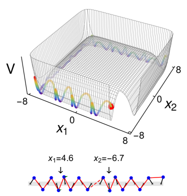
(a)

(b)

(c)

(d)

Figure 19: The trajectories of the chain generated by simulations of Newtonian dynamics on the theoretical potential function in the configuration space at (a) $l_{0}<l_{critical}$, $E<E_{c}$, (b) $l_{0}<l_{critical}$, $E>E_{c}$, (c) $l_{0}=l_{critical}$, $E=E_{c}=0$, and (d) $l_{0}>l_{critical}$. In the top figures of (a) and (b), the color scale of the trajectories indicates the potential energy of the chain in arbitrary units. The big red dots correspond to the configuration of the real-space chains shown in the bottom figures of each panel.

The phase space of a chain with two kinks is 4D. For the convenience of visualization, we investigate the potential function $V(x_{1},x_{2};l_{0})$ in the 2D configuration space. The shape of the potential depends on $l_{0}$ and determines the qualitative dynamics of the two kinks. We also perform simulations of Newtonian dynamics to investigate the qualitative behavior of the nonlinear motion of the kinks.

When $l_{0}<l_{critical}$ (Fig. 19a), the potential looks like a square Mexican hat. The bottom of potential valley is a square ring, on which all the points are at zero energy. In linear mode analysis, we find a zero mode along the valley and a soft mode along the transverse direction. We will show that the nonlinear dynamics at finite energy possesses the traits that are closely related to those in the linear analysis at zero energy.

Note that the impurity spring is maximally stretched at $x_{1}=x_{2}=0$, and the corresponding potential maximum $E_{c}=\frac{1}{2}k(l_{0}-l_{critical})^{2}$. It is the minimal energy for both kinks to move away from the impurity. If $E<E_{c}$, the two kinks take turns moving on their respective sub-chains. One kink oscillates near the impurity spring, while the other kink moves away. The nonlinear dynamics of the kinks is visualized as a trajectory going along the bottom of the potential valley. The accessible region in the configuration space is a square annulus, at the corner of which the major part of energy is transferred from the one kink to another. In fact, this can be interpreted as the motion of a single “split” kink through the system.

When $E\geq E_{c}$ (Fig. 19b), there is sufficient energy for both kinks to move away from the impurity spring simultaneously. In the configuration space, the trajectory gets out of the potential valley and climbs up to the 2D plateau in the middle. The accessible region now is a square disk. In real space, the kinks independently hit the impurity spring and get reflected.

When $l_{0}=l_{critical}$ (Fig. 19c), the linear mode analysis predicts that the chain model in Fig. 19c has two zero modes, each being localized around the kink at the end of the respective sub-chain, and a state of self stress localized around the impurity spring. From the viewpoint of nonlinear dynamics, the potential function changes qualitatively: As $l_{0}$ approaches $l_{critical}$, the square ring of the potential valley shrinks into one point at $x_{1}=x_{2}=0$, and $E_{c}$ goes to zero. In other words, the Mexican hat transforms into a single basin. In this shrinking process, the soft mode, which corresponds to the oscillation transverse to the valley, transitions into a zero mode, because the depth of the valley vanishes. In terms of nonlinear dynamics, this transition means that no matter how small the total energy $E$ is, the accessible region in the configuration space is always a square disk rather than a square annulus.

When $l_{0}>l_{critical}$ (Fig. 19d), the impurity spring is compressed, which gives a minimum potential energy $E_{min}=\frac{1}{2}k(l_{0}-l_{critical})^{2}$ for the static configuration. In a linear analysis, the two zero modes become normal modes with finite frequency, as the impurity spring pushes the two kinks to the chain ends, generating a finite restoring force for the motion of the modes. In the nonlinear dynamics, the accessible region of the kinks is still a square disk.

Figure 20: The parameter space of the total energy $E$ and the impurity spring length $l_{0}$. The critical energy $E_{c}$ as a function of $l_{0}$ forms a parabola. The chain shows different dynamical behaviors across the left branch of the parabola. The vertical dashed line of $l_{0}=l_{critical}$ is the boundary line across which the shape of the potential function transitions qualitatively. The gray area below the right branch of the parabola is energetically forbidden.

Fig. 20 summarizes the above results with $E$ and $l_{0}$ as parameters. When $l_{0}\leq l_{critical}$, the curve $E_{c}=\frac{1}{2}k(l_{0}-l_{critical})^{2}$ marks the transition of the accessible region in configuration space from an annulus to a disk. Note that we only investigate the case of $l_{0}>\overline{l}$, in which Fig. 20 is valid. For $l_{0}<\overline{l}$ case, the potential landscape takes a different form, and so does the possible transition. We do not cover this case in this paper, however, as we have made the connection between linear mode analysis and nonlinear dynamics.

VIII Conclusion

We have studied the nonlinear dynamics of a topological rotor chain. The continuum limit is well-approximated by a modified $\phi^{4}$ theory whose nonlinear excitations are the kinks and antikinks. We have seen how the breaking of inversion asymmetry at the discrete level results in an asymmetry between the kink and antikink excitations that affects the properties of linear modes around these excitations, their transport along an ordered lattice as well as in how these excitations interact with a lattice impurity. The results herein further enrich the class of phenomenon described by the $\phi^{4}$ theory, a model which is extensively studied and finds numerous applications in many fields of physics.

Some questions for further research – (1) We find that kinks reflect perfectly off the free boundaries of a topological rotor chain. This is surprising given that in the continuum limit, the $\phi^{4}$ kink is a non-integrable solution and thus could create bound states or emit radiation as it interacts with a free boundary. Furthermore, an antikink cannot reach a free boundary without colliding with a kink – another feature which we do not yet know how to interpret within the continuum theory. (2) We have not undertaken a detailed study of the phases of motion for an antikink (wobbling, spinner). Preliminary simulations indicate that antikink configurations in these other phases are in fact unstable. The large amount of initial spring stretching energy necessary in a configuration where the rotors point “away from each other” is immediately converted to kinetic energy and induces rapid spinning of the nearby rotors which then spreads across the system in a chaotic fashion. It is not clear how this effect would arise in the continuum theory, which for the spinner, is related to the integrable sine-Gordon model Chen et al. (2014).

A more speculative question is whether there are connections between our results and the observed asymmetry between kinks and antikinks in certain one-dimensional quantum magnetic systems, called delta or sawtooth chains Nakamura and Kubo (1996); Sen et al. (1996). These systems also have two uniform ground states which may be thought of as the analog of “right-leaning” and “left-leaning” states, and also share the property that the excitation energy for a kink is zero while for an antikink is large and finite.

Appendix A Complex notation

We use complex variables to derive the explicit relation between neighbouring rotor angles. Adopting the notation in Fig. 1c, we put the pivot of rotor 1 at the origin of complex plane and the pivot of rotor 2 at the coordinate (a,0). The positions of the rotor tips are

$$z_{1} =ire^{-i\theta_{1}},$$ (21)

$$z_{2} =a-ire^{i\theta_{2}}.$$ (22)

We have two constraints (where a bar represents complex conjugations):

$$(z_{2}-z_{1})(\bar{z}_{2}-\bar{z}_{1})=l^{2}_{0},$$ (23)

$$(z_{2}-a)(\bar{z}_{2}-a)=r^{2}.$$ (24)

Eliminating $\bar{z}_{2}$ from above two constraints, we find a quadratic equation for $z_{2}$,

$$Az^{2}_{2}+Bz_{2}+C=0,$$ (25)

where

$$A =\frac{\bar{z}_{1}-a}{a-z_{1}},$$ (26)

$$B =\left(\frac{l^{2}_{0}+a^{2}-2r^{2}}{a-z_{1}}\right)-a\left(\frac{\bar{z}_{1}-z_{1}}{a-z_{1}}\right),$$ (27)

$$C =a^{2}-r^{2}-a\left(\frac{l^{2}_{0}+a^{2}-2r^{2}}{a-z_{1}}\right).$$ (28)

We have two branches of the solution for $z_{2}$

$$z_{2}=\frac{-B\pm\sqrt{B^{2}-4AC}}{2A},$$ (29)

which explicitly expresses the black curve in Fig. 3b.

Appendix B Vibrational modes of prestressed mechanical structures: Method of Tangent stiffness matrix

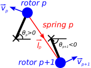
(a)

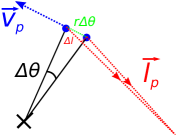
(b)

Figure 21: Detailed configurations around a single spring $p$.

Consider a single spring $p$ in the configuration shown in Fig. 21a (note here, we are now specifying rotor angles $\theta$ with respect to the positive $x$-axis). From geometry, we find

$$\begin{split}f_{p}&=-\vec{v}_{p}\cdot\vec{l}_{p}~{}~{}\hat{t}_{p}\\ f_{p+1}&=\vec{v}_{p+1}\cdot\vec{l}_{p}~{}~{}\hat{t}_{p}.\end{split}$$ (30)

Here, $f_{p}$ is the spring force projected along the tangent vector $\vec{v}_{p}$ of rotor $p$

$$\begin{split}\vec{v}_{p}=\begin{pmatrix}-\sin\theta_{p}\\ \cos\theta_{p}\end{pmatrix}.\end{split}$$ (31)

$\vec{l}_{p}$ is the vector along the length of the spring $p$ and points from rotor $p$ to $p+1$,

$$\begin{split}\vec{l}_{p}=\begin{pmatrix}a+r\cos\theta_{p+1}-r\cos\theta_{p}\\ r\sin\theta_{p+1}-r\sin\theta_{p}\end{pmatrix}.\end{split}$$ (32)

$\hat{t}_{p}$ is a scalar tension coefficient for spring $p$, defined as $\hat{t}_{p}\equiv t_{p}/|\vec{l}_{p}|$, where $t_{p}\equiv k_{p}(|\vec{l}_{p}|-\overline{l})$ for a harmonic spring. Here, $|\vec{l}_{p}|$ is the instantaneous length of spring $p$, $\overline{l}$ is the rest length of the spring, and $k$ is the spring constant.

In order to find the tangent stiffness, we differentiate Eqn. (30) with respect to the rotor angles $\theta_{p}$ and $\theta_{p+1}$

$$\begin{split}\frac{\partial f_{p}}{r\partial\theta_{p}}&=\frac{\partial(-\vec{v}_{p}\cdot\vec{l}_{p})}{r\partial\theta_{p}}~{}~{}\hat{t}_{p}-\vec{v}_{p}\cdot\vec{l}_{p}~{}\frac{\partial\hat{t}_{p}}{r\partial\theta_{p}}\end{split}$$ (33)

$$\begin{split}\frac{\partial f_{p}}{r\partial\theta_{p+1}}&=\frac{\partial(-\vec{v}_{p}\cdot\vec{l}_{p})p}{r\partial\theta_{p+1}}~{}~{}\hat{t}_{p}-\vec{v}_{p}\cdot\vec{l}_{p}~{}\frac{\partial\hat{t}_{p}}{r\partial\theta_{p+1}}\end{split}$$ (34)

$$\begin{split}\frac{\partial f_{p+1}}{r\partial\theta_{p}}&=\frac{\partial(\vec{v}_{p+1}\cdot\vec{l}_{p})}{r\partial\theta_{p}}~{}~{}\hat{t}_{p}+\vec{v}_{p+1}\cdot\vec{l}_{p}~{}\frac{\partial\hat{t}_{p}}{r\partial\theta_{p}}\end{split}$$ (35)

$$\begin{split}\frac{\partial f_{p+1}}{r\partial\theta_{p+1}}&=\frac{\partial(\vec{v}_{p+1}\cdot\vec{l}_{p})}{r\partial\theta_{p+1}}~{}~{}\hat{t}_{p}+\vec{v}_{p+1}\cdot\vec{l}_{p}~{}\frac{\partial\hat{t}_{p}}{r\partial\theta_{p+1}}.\end{split}$$ (36)

To simplify Eqn. (33), we express

$$\begin{split}\frac{\partial\hat{t}_{p}}{r\partial\theta_{p}}&=\frac{\mathrm{d}\hat{t}_{p}}{\mathrm{d}|\vec{l}_{p}|}~{}\frac{\partial|\vec{l}_{p}|}{r\partial\theta_{p}}\end{split}$$ (37)

$$\begin{split}\frac{\mathrm{d}\hat{t}_{p}}{\mathrm{d}|\vec{l}_{p}|}&=\frac{\mathrm{d}(t_{p}/|\vec{l}_{p}|)}{\mathrm{d}|\vec{l}_{p}|}=\frac{1}{|\vec{l}_{p}|}(g_{p}-\hat{t}_{p})=\hat{g}_{p}/|\vec{l}_{p}|,\end{split}$$ (38)

where $g_{p}\equiv\mathrm{d}t_{p}/d|\vec{l}_{p}|$ is defined as the axial stiffness and $\hat{g}_{p}\equiv g_{p}-\hat{t}_{p}$ is defined as the modified axial stiffness.

From Fig. 21b, we see that $\Delta l=r\Delta\theta~{}(-\vec{v}_{p}\cdot\vec{l}_{p})/|\vec{l}_{p}|$ and therefore,

$$\begin{split}\frac{\partial|\vec{l}_{p}|}{r\partial\theta_{p}}=\frac{(-\vec{v}_{p}\cdot\vec{l}_{p})}{|\vec{l}_{p}|}\end{split}$$ (39)

Substituting Eqn. (37 - 39) into Eqn. (33), we find

$$\begin{split}\frac{\partial f_{p}}{r\partial\theta_{p}}&=\frac{\partial(-\vec{v}_{p}\cdot\vec{l}_{p})}{r\partial\theta_{p}}~{}~{}\hat{t}_{p}-(\vec{v}_{p}\cdot\vec{l}_{p})~{}\frac{\hat{g}_{p}}{|\vec{l}_{p}|}\frac{(-\vec{v}_{p}\cdot\vec{l}_{p})}{|\vec{l}_{p}|}.\end{split}$$ (40)

Similarly, we simplify Eqns. (34 - 36)

With the above derivatives, we can now define the tangent stiffness matrix. For a single spring $p$, the tangent stiffness matrix, $\mathbf{K}_{p}$, relates small changes in rotor position to small changes in rotor forces

$$\begin{split}\begin{pmatrix}\delta f_{p}\\ \delta f_{p+1}\end{pmatrix}=\mathbf{K}_{p}\begin{pmatrix}r\delta\theta_{p}\\ r\delta\theta_{p+1}\end{pmatrix}\end{split}$$ (41)

and can be expressed as

$$\begin{split}\mathbf{K}_{p}=\begin{pmatrix}n_{p}\\ n_{p+1}\end{pmatrix}\Big{[}\hat{g}_{p}\Big{]}\begin{pmatrix}n_{p}&n_{p+1}\end{pmatrix}+\mathbf{s_{p}},\end{split}$$ (42)

where $n_{p}\equiv-\vec{v}_{p}\cdot\vec{l}_{p}/|\vec{l}_{p}|$, $n_{p+1}\equiv-\vec{v}_{p+1}\cdot\vec{l}_{p}/|\vec{l}_{p}|$ and the stress matrix $\mathbf{s}_{p}$ is

$$\begin{split}\mathbf{s}_{p}=\begin{pmatrix}-\frac{\partial(\vec{v}_{p}\cdot\vec{l}_{p})}{r\partial\theta_{p}}~{}\hat{t}_{p}&~{}~{}-\frac{\partial(\vec{v}_{p}\cdot\vec{l}_{p})}{r\partial\theta_{p+1}}~{}\hat{t}_{p}\\ \\ \frac{\partial(\vec{v}_{p+1}\cdot\vec{l}_{p})}{r\partial\theta_{p}}~{}\hat{t}_{p}&~{}~{}\frac{\partial(\vec{v}_{p+1}\cdot\vec{l}_{p})}{r\partial\theta_{p+1}}~{}\hat{t}_{p}\end{pmatrix}.\end{split}$$ (43)

To derive the total tangent stiffness $\mathbf{K}$ for the rotor chain, we first represent the tangent stiffness $\mathbf{K}_{p}$ in a global coordinate system as an $n\times n$ matrix, and then sum up all the $\mathbf{K}_{p}$ for the $n-1$ springs:

$$\begin{split}\mathbf{K}=\sum_{p=1}^{n-1}\mathbf{K}_{p}=\sum_{p=1}^{n-1}\mathbf{a}_{p}\big{[}\hat{g}_{p}\big{]}\mathbf{a}_{p}^{T}+\sum_{p=1}^{n-1}\mathbf{S}_{p},\end{split}$$ (44)

where

$$\begin{split}\mathbf{a}_{p}=\begin{pmatrix}0\\ \vdots\\ 0\\ n_{p}\\ n_{p+1}\\ 0\\ \vdots\\ 0\end{pmatrix}\end{split}$$ (45)

and

$$\begin{split}\mathbf{S}_{p}=\begin{pmatrix}\text{\huge 0}&~{}~{}~{}~{}~{}~{}\ldots&&\text{\huge 0}\\ \vdots&\mathbf{s}_{p11}~{}&\mathbf{s}_{p12}~{}&\vdots\\ \vdots&\mathbf{s}_{p11}~{}&\mathbf{s}_{p12}~{}&\vdots\\ \text{\huge 0}&~{}~{}~{}~{}~{}~{}\ldots&&\text{\huge 0}\end{pmatrix}.\end{split}$$ (46)

In $\mathbf{a}_{p}$, the $n_{p}$ and $n_{p+1}$ terms are in the $p$th and $p+1$th row respectively, and all the other terms are zero. In $\mathbf{S}_{p}$, $\mathbf{s}_{pij}$ is the $(i,j)$ element of the $2\times 2$ stress matrix $\mathbf{s}_{p}$ for a single spring $p$ and is located in the $(p-1+i,p-1+j)$ position of $\mathbf{S}_{p}$, and all the other terms in $\mathbf{S}_{p}$ are zero. Here $\mathbf{S}_{p}$ has a simpler form than that of Ref. Guest (2006) because we exploit the fact that only nearest neighbours are coupled in the topological chain.

Appendix C Simulation methods

The molecular dynamics simulations are carried out in Mathematica. The ODEs are solved by the function NDSolve, which uses a multi-step method (LSODA) by default.

In the simulations, we set the lattice spacing $a=1$, the rotor mass $M=1$, and an arbitrary time unit $t=1$. The spring constant $k$ is measured in units of $M/t^{2}$. The linear velocity of a rotor is measured in units of $a/t$. The initial velocity $v_{0}$ of a (anti)kink is defined as the velocity amplitude of the unit translation mode ${\bf e}^{t}$ and $e^{t}_{i}$ is the mode component on the $i$-th rotor. Thus the initial kinetic energy is $\Sigma_{i}\frac{1}{2}m(v_{0}e^{t}_{i})^{2}=\frac{1}{2}mv_{0}^{2}$.

Appendix D Peierls-Nabarro potential barrier via continuum theory

We derive the PN potential by discretizing the potential energy density in the continuum theory, i.e. taking the quasi-continuum limit. The PN potential is, by definition, the potential that the kink faces as it propagates along the adiabatic trajectory (ad. tr.) :

$$\begin{split}V_{PN}(X)&=V(...,u_{n-1},u_{n},u_{n+1},...)|_{X\in ad.tr.}.\end{split}$$ (47)

Here, $X$ is the position of the (anti)kink center, $u_{n}$ is the continuum field at lattice site $n$, $V$ is a discretization of the potential energy density $V(\theta)$ in Eqn. (9) and is obtained by summing the potential $f(n,X)$ of each lattice site:

$$\begin{split}V(...,u_{n-1},u_{n},u_{n+1},...)&=\sum f(n,X),\end{split}$$ (48)

where

$$\begin{split}f(n,X)&=\frac{2k}{\overline{l}^{2}}\left(\frac{a^{2}}{2}\frac{\mathrm{d}u_{n}}{\mathrm{d}(na)}+\overline{u}^{2}-u^{2}_{n}\right)^{2}.\end{split}$$ (49)

$f(n,X)$ is the approximate potential at a single site $n$ when the (anti)kink center is at $X$. Here, we discretize the continuum potential energy density rather than directly use the exact form of the lattice potential in Eqn. (8), so that we can readily substitute $u_{n}$, the continuum field at site $n$, into $f(n,X)$ which results in an integrable solution. We choose the static solution ($v=0$) of Eqn. (13) as the adiabatic trajectory:

$$\begin{split}u_{n}(X)=\pm\overline{u}\tanh\Big{(}\frac{na-X}{w}\Big{)},\end{split}$$ (50)

where the “$+$” is for the antikink, “$-$” is for the kink, and the width of the (anti)kink $w=\frac{a^{2}}{2r\sin\overline{\theta}}$ Chen et al. (2014). Substituting Eqn. (50) into Eqn. (49), we find

$$\begin{split}f(n,X)&=0~{}~{}~{}~{}~{}~{}~{}~{}~{}~{}~{}~{}~{}~{}~{}~{}~{}~{}~{}~{}~{}~{}~{}~{}~{}~{}~{}~{}~{}\textrm{for the kink,}\\ f(n,X)&=\frac{8k\overline{u}^{4}}{\overline{l}^{2}}\operatorname{sech}^{4}\Big{(}\frac{na-X}{w}\Big{)}~{}~{}\textrm{for the antikink.}\end{split}$$ (51)

Thus $V_{PN}(X)=0$ for the kink, in accordance with the fact that the kink configuration does not stretch springs and hence costs zero potential energy. For the antikink, we use the Poisson summation formula to express:

$$\begin{split}V_{PN}(X)&=\sum_{n=-\infty}^{+\infty}f(n,X)=\sum_{k=-\infty}^{+\infty}\hat{f}(k,X)\\ &=\sum_{k=-\infty}^{+\infty}\int_{-\infty}^{+\infty}\mathrm{d}nf(n,X)e^{-2\pi ikn}.\end{split}$$ (52)

To leading order, we only consider the first harmonic terms $k=1$ and $k=-1$ ($k=0$ recovers the continuum approximation). For $k=1$, we find

$$\begin{split}&~{}~{}\int_{-\infty}^{+\infty}\mathrm{d}nf(n,X)e^{-2\pi in}\\ &=e^{-2\pi i(X/a)}\int_{-\infty}^{+\infty}\mathrm{d}n^{\prime}\frac{8k\overline{u}^{4}}{\overline{l}^{2}}\operatorname{sech}^{4}\Big{(}\frac{n^{\prime}a}{w}\Big{)}e^{-2\pi in^{\prime}}.\end{split}$$ (53)

The complex exponential suggests a sinusoidally varying potential along the coordinate $X$ of the adiabatic trajectory, with a period that is equal to the lattice spacing $a$. We define the PN barrier ($V_{PNB}$) as the height of this sinusoidal potential. The last integral in Eqn. (53) can be completed using residues to yield

$$\begin{split}V_{PNB}&=\frac{4\pi^{2}\big{(}\pi^{2}+(a/w)^{2}\big{)}}{3\big{(}1+4(r/a)^{2}-(a/w)^{2}\big{)}\sinh(\pi^{2}w/a)}\\ &\propto e^{-\pi^{2}w/a}~{}~{}~{}~{}~{}~{}~{}~{}~{}~{}~{}~{}\textrm{for large $w/a$.}\end{split}$$ (54)

Appendix E Definition of kink coordinates in discrete models

The concept of kinks stems from the continuum $\phi^{4}$ theory. To extend this concept to the discrete chain model, we define the coordinate system of a sub-chain kink as follows (Fig. 18a): The absolute value of the position of a kink equals the rotor’s integer index if the rotor is vertical, otherwise the position is a real number interpolating between the indices of the two neighboring rotors that are leaning opposite to each other. The positional interpolation is proportional to the linear interpolation between the absolute values of the angles of two neighbor rotors. The rotor angles are the measured against the vertical alternatively, as mentioned in Section II. When a kink approaches the end points of the chain, the end rotor flips over. Here the kink profile from the continuum theory ceases to be valid. Thus we take as our convention that a kink is at the origin of the coordinate system when the end rotor is collinear with the spring connecting to the next rotor, and its sign depends on whether the end rotor leans upwards or downwards. The coordinate between $0$ and $1$ (or $-2$) is obtained by linear interpolation of the angles of the end rotor at $0$ and $1$ (or $-2$). In this ad hoc convention, the chain forms a state of self stress when both kinks are at origin. The two sub-chains are aligned head-to-head, and the two head rotors ($|x_{i}|=8$) are coupled by the impurity spring.

References

- Hasan and Kane (2010) M. Z. Hasan and C. L. Kane, Reviews of Modern Physics 82, 3045 (2010).
- Prodan and Prodan (2009) E. Prodan and C. Prodan, Physical Review Letters 103, 248101 (2009).
- Berg et al. (2011) N. Berg, K. Joel, M. Koolyk, and E. Prodan, Physical Review E 83, 021913 (2011).
- Susstrunk and Huber (2015) R. Susstrunk and S. D. Huber, Science 349, 47 (2015).
- Süsstrunk and Huber (2016) R. Süsstrunk and S. D. Huber, arXiv preprint (2016), arXiv:1604.01033 .
- Wang et al. (2015a) Y.-T. Wang, P.-G. Luan, and S. Zhang, New Journal of Physics 17, 073031 (2015a).
- Wang et al. (2015b) P. Wang, L. Lu, and K. Bertoldi, Physical Review Letters 115, 104302 (2015b).
- Mousavi et al. (2015) S. H. Mousavi, A. B. Khanikaev, and Z. Wang, Nature Communications 6, 8682 (2015).
- Khanikaev et al. (2015) A. B. Khanikaev, R. Fleury, S. H. Mousavi, and A. Alù, Nature Communications 6, 8260 (2015).
- Nash et al. (2015) L. M. Nash, D. Kleckner, A. Read, V. Vitelli, A. M. Turner, and W. T. M. Irvine, Proceedings of the National Academy of Sciences of the United States of America 112, 14495 (2015).
- Yang et al. (2015a) Z. Yang, F. Gao, X. Shi, X. Lin, Z. Gao, Y. Chong, and B. Zhang, Physical Review Letters 114, 1 (2015a).
- Yang et al. (2015b) Z. Yang, F. Gao, and B. Zhang, arXiv preprint (2015b), arXiv:1504.02655 .
- Xiao et al. (2015) M. Xiao, W.-J. Chen, W.-Y. He, and C. T. Chan, Nature Physics 11, 920 (2015).
- Peano et al. (2015) V. Peano, C. Brendel, M. Schmidt, and F. Marquardt, Physical Review X 5, 031011 (2015).
- Kariyado and Hatsugai (2015) T. Kariyado and Y. Hatsugai, Scientific Reports 5, 18107 (2015).
- Deymier et al. (2015) P. A. Deymier, K. Runge, N. Swinteck, and K. Muralidharan, Comptes Rendus Mécanique 1, 1 (2015).
- Bi and Wang (2015) R. Bi and Z. Wang, arXiv preprint (2015), arXiv:1508.04896v1 .
- Po et al. (2014) H. C. Po, Y. Bahri, and A. Vishwanath, arXiv preprint (2014), arXiv:1410.1320 .
- Lawler (2015) M. J. Lawler, arXiv preprint (2015), arXiv:1510.03697 .
- Kane and Lubensky (2013) C. L. Kane and T. C. Lubensky, Nature Physics 10, 39 (2013).
- Lubensky et al. (2015) T. C. Lubensky, C. L. Kane, X. Mao, A. Souslov, and K. Sun, Reports on Progress in Physics 78, 073901 (2015).
- Vitelli (2012) V. Vitelli, Proceedings of the National Academy of Sciences of the United States of America 109, 12266 (2012).
- Chen et al. (2014) B. G. Chen, N. Upadhyaya, and V. Vitelli, Proceedings of the National Academy of Sciences of the United States of America 111, 8 (2014).
- Vitelli et al. (2014) V. Vitelli, N. Upadhyaya, and B. G. Chen, arXiv preprint (2014), arXiv:1407.2890 .
- Meeussen et al. (2016) A. S. Meeussen, J. Paulose, and V. Vitelli, arXiv preprint (2016), arXiv:1602.08769 .
- Paulose et al. (2015a) J. Paulose, B. G. Chen, and V. Vitelli, Nature Physics 11, 153 (2015a).
- Chen et al. (2016) B. G. Chen, B. Liu, A. A. Evans, J. Paulose, I. Cohen, V. Vitelli, and C. Santangelo, Physical Review Letters 116, 135501 (2016).
- Rocklin et al. (2015) D. Z. Rocklin, S. Zhou, K. Sun, and X. Mao, arXiv preprint (2015), arXiv:1510.06389 .
- Rocklin et al. (2016) D. Z. Rocklin, B. G. Chen, M. Falk, V. Vitelli, and T. C. Lubensky, Physical review letters 116, 135503 (2016).
- Paulose et al. (2015b) J. Paulose, A. S. Meeussen, and V. Vitelli, Proceedings of the National Academy of Sciences of the United States of America 112, 7639 (2015b).
- Maxwell (1864) J. C. Maxwell, Philosophical Magazine Series 4 27, 294 (1864).
- Calladine (1978) C. Calladine, International Journal of Solids and Structures 14, 161 (1978).
- Manton and Sutcliffe (2004) N. Manton and P. Sutcliffe, Topological Solitons (Cambridge University Press, 2004).
- Guest (2006) S. Guest, International Journal of Solids and Structures 43, 842 (2006).
- Combs and Yip (1983) J. A. Combs and S. Yip, Physical Review B 28, 6873 (1983).
- Braun and Kivshar (1998) O. M. Braun and Y. S. Kivshar, Physics Reports 306, 1 (1998).
- Roy et al. (2007) I. Roy, S. V. Dmitriev, P. G. Kevrekidis, and A. Saxena, Phys. Rev. E 76, 26601 (2007).
- Fraggis et al. (1989) T. Fraggis, S. Pnevmatikos, and E. Economou, Physics Letters A 142, 361 (1989).
- Fei et al. (1992) Z. Fei, Y. S. Kivshar, and L. Vázquez, Phys. Rev. A 46, 5214 (1992).
- Note (1) Varying the parameters () yield other phases of the topological rotor chain. In this work, we only consider the topological chain in the flipper phase Chen et al. (2014) where the theory is a valid approximation. The name flipper describes the back-and-forth motion of the rotors as a kink propagates, in contrast to the spinner phase, where the rotors complete a full circle. The continuum limit of the spinner phase can be approximately described by the sine-Gordon theory.
- Campbell et al. (1983) D. K. Campbell, J. F. Schonfeld, and C. A. Wingate, Physica D: Nonlinear Phenomena 9, 1 (1983).
- Makhankov (1990) V. Makhankov, Soliton Phenomenology (Springer Netherlands, 1990).
- Note (2) In the language of dynamical systems, this process is called a supercritical pitchfork bifurcation.
- Nakamura and Kubo (1996) T. Nakamura and K. Kubo, Physical Review B 53, 6393 (1996).
- Sen et al. (1996) D. Sen, B. S. Shastry, R. E. Walstedt, and R. Cava, Physical Review B 53, 6401 (1996).