Extended friction elucidates the breakdown of fast water transport in graphene oxide membranes

Abstract

The understanding of water transport in graphene oxide (GO) membranes stands out as a major theoretical problem in graphene research. Notwithstanding the intense efforts devoted to the subject in the recent years, a consolidated picture of water transport in GO membranes is yet to emerge.

By performing mesoscale simulations of water transport in ultrathin GO membranes, we show that even small amounts of oxygen functionalities can lead to a dramatic drop of the GO permeability, in line with experimental findings.

The coexistence of bulk viscous dissipation and spatially extended molecular friction results in a major decrease of both slip and bulk flow, thereby suppressing the fast water transport regime observed in pristine graphene nanochannels.

Inspection of the flow structure reveals an inverted curvature in the near-wall region, which connects smoothly with a parabolic profile in the bulk region. Such inverted curvature is a distinctive signature of the coexistence between single-particle Langevin friction and collective hydrodynamics.

The present mesoscopic model with spatially extended friction may offer a computationally efficient tool for future simulations of water transport in nanomaterials.

Water transport through graphene-derived membranes has recently captured much attention due to its promising potential for many technological applications, such as water filtration, separation processes, and heterogeneous catalysis Cohen-Tanugi and Grossman (2012); Mishra and Ramaprabhu (2011); Julkapli and Bagheri (2015); Garberoglio et al. (2007). A number of simulations have shown that fast water permeation through carbon materials, such as carbon nanotubes (CNT Joseph and Aluru (2008); Holt et al. (2006); Zuo et al. (2009); Majumder et al. (2005)) and pristine graphene membranes Nair et al. (2012) is due to the slip flow at the water-carbon interface. Fast water transport (FWT) with permeabilities higher than $10\;Lm^{-2}h^{-1}bar^{-1}$ Hu and Mi (2013); Jiang et al. (2015); Han et al. (2013) has also been reported for graphene oxide laminate (GOL).
However, in contrast to pristine graphene and CNT, a clear consensus on the GOL fast water transport mechanism has yet to emerge Nair et al. (2012); Huang et al. (2013); Sun et al. (2016). To date, departures from hydrodynamic (i.e., Hagen-Poiseuille) behavior are typically attributed to the low friction experienced by water in atomistically smooth graphene nanochannels Joshi et al. (2014) or to the presence of structural defects in GOL, leading to shorter water paths Wei et al. (2014a); Joseph and Aluru (2008). The latter hypothesis is further corroborated by the breakdown of FWT from molecular interactions of water with basal plane hydroxide and epoxide groups, which hinders the motion of water molecules. This phenomenon was recently reported in non-equilibrium molecular dynamics simulations of flows inside graphene oxide (GO) nanochannels, Wei et al. (2014a, b). Under such conditions, slip-corrected continuum hydrodynamics is expected to provide a correct description of the aforementioned transport mechanism. However, at the hydrodynamic level the details of the slip corrections must be imposed a priori because the physics of slip flow is governed by non-equilibrium phenomena. Such details can certainly be accounted for by a fully atomistic approach, but at the price of prohibitive computational costs. All of the above lead to an ideal scenario for mesoscale modeling techniques, which may offer a valuable compromise between physical fidelity and computational viability, Montessori et al. (2015).
In this work, we explore water permeation in GOL via mesoscale simulations. Furthermore, we provide a direct calculation of the membrane’s permeability, which is drastically lower than the one observed in pristine graphene characterized by FWT. Our simulations exhibit satisfactory agreement with experimental GOL permeability and also provide values of the slip length on par with recent non-equilibrium molecular dynamics simulations (NEMD) Wei et al. (2014b). More precisely, we demonstrate that a suitably simplified (lattice) kinetic model proves capable of predicting the breakdown of FWT, namely the macroscopic permeability of the GO membrane, as well as the slip phenomena, at a very affordable computational cost. For instance, a baseline simulation takes only a few CPU hours on a high-end PC.

Figure 1: Sketch of the GOL structure with a zoom of the GO nanochannel decorated with oxygen functionalities (panel (a)). In the sketch, L is the GO flake’s length, $2h$ is the spacing between two GO layers and w is the spatial extent of the Langevin-like frictional force. The red area in the GOL structure identifies the elementary periodic cell used in the simulation. As shown in panel (b), hydroxide abd epoxide groups interact with the water molecules slowing down their motion inside the GO nanochannels. In panel (c), the water molecules flow from the inlet port (top) to the outlet port (bottom), under the effect of applied pressure. The vertical motion is hindered by a series of horizontal staggered plates (GO flakes), which force the water molecules to follow a tortuous path from inlet to outlet ports.

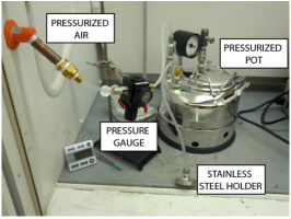
Method. GO was synthesized by modified Hummers’ method Kovtyukhova et al. (1999) and dispersed in ethanol at a concentration of $0.1\;mg/L$. Additional details can be found in the supporting information. The solution was then bath sonicated for 5 minute in a Branson 2510 Ultrasonic cleaner. $1\;ml$ of the sonicated GO solution was deposited on a porous polyvinylidene difluoride (PVDF) membrane (pore size = $200\;nm$) via vacuum filtration. The membranes were then characterized by using a Zeiss ULTRA Field Emission Scanning Electron Microscope (SEM) with an In-lens detector (see Figure S 1 and S 2 in the supporting information). Scanning electron microscopy and mass analysis suggest the formation of a circa $30\;nm$ thick GO layer on top of the PVDF membrane. The crystallographic structure of the membranes was analyzed with a Bruker D8 equipped with a two-dimensional VANTEC-500 detector. The spectra were obtained by the integration of the 2D diffraction pattern image (see Figure S 3 in the supporting information) via EVA software. Depending on the sample, the integration time was between 600-1200 seconds. Permeability results were carried out with a custom-made dead-end filtration system operating at a maximum pressure of $3.5\;bar$. In particular, a $2\;cm$ in diameter GO membrane was cut and placed in a stainless steel EDM Millipore filter holder. The pressure was monitored with an Ingersoll pressure gauge regulator (see Figure S 4 in the supporting information). The numerical simulations are based on the Lattice Boltzmann (LB) method, augmented with a novel Langevin-like frictional force accounting for the GO-water interactions. Since the LB method is largely documented in the literature Qian et al. (1992); Higuera et al. (1989); Succi (2015), in the following we discuss only its basic features. The lattice Boltzmann equation reads as follows:

$$f_{i}(\vec{x}+\vec{c}_{i}\Delta t,t+\Delta t)=(1-1/\tau)f_{i}+1/\tau f_{i}^{e}+\Delta f_{i}$$ (1)

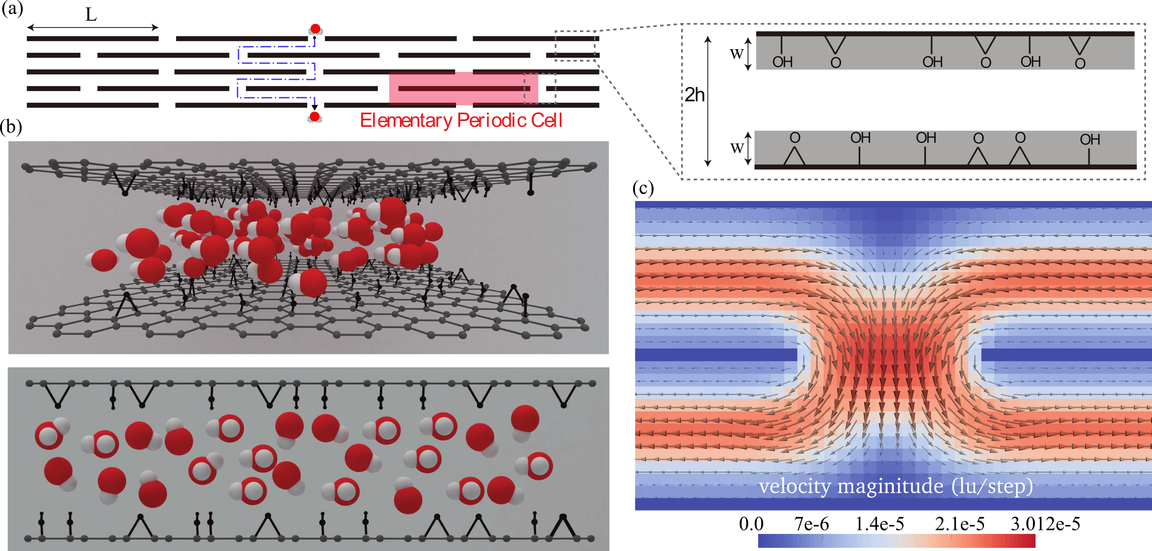
where $f_{i}(\vec{x},t)$ is a set of discrete probability distribution functions (PDFs) representing the probability of finding a molecule at position $\vec{x}$ and time $t$ with a lattice-constrained velocity $\vec{c}_{i}$, where the index $i$ runs over the nine directions of the lattice Succi (2001). $f_{i}^{e}$ is the set of discrete local Maxwellian equilibria (i.e., truncated low-Mach number expansion of the Maxwell-Boltzmann distribution) Qian et al. (1992) and $c_{s}$ is the speed of sound of the model Succi (2001); Wolf-Gladrow (2000). In the above equation, the left hand side is the lattice transcription of molecular free-flight along the lattice directions, while the right hand side describes collisional relaxation towards local equilibrium, described by a low-Mach number expansion of the Maxwell-Boltzmann distribution. The relaxation parameter $\tau$ controls the kinematic viscosity of the lattice fluid through the relation $\nu=c_{s}^{2}(\tau-1/2)$ in lattice units $\Delta x=\Delta t=1$. The last term, $\Delta f_{i}$, is the correction due to the friction exerted by the hydroxyl and epoxy (see Fig. 1b) on the water molecules and can be expressed as: $\Delta f_{i}=w_{i}\frac{\vec{F}\cdot\vec{c_{i}}}{c_{s}^{2}}$, in which $w_{i}$ is the set of weights for the chosen lattice Qian et al. (1992), and the frictional force is taken in the following Langevin form Smiatek et al. (2008):

$$\vec{F}=-\rho\gamma(y)\vec{u}$$ (2)

where $\rho$ and $\vec{u}$ are the fluid density and velocity respectively and the heterogeneous friction coefficient reads as follows:

$$\gamma(y)=\gamma_{0}(e^{-\frac{y}{\text{w}}}H_{L}(y,\delta)+e^{\frac{(y-h)}{\text{w}}}H_{R}(y,\delta))$$ (3)

where w is a representative size of the protruding functional groups and $\gamma_{0}$ is a characteristic water-hydroxyl collision frequency, taken equal to $0.2$ (in lattice units) in all the simulations, corresponding to a collision rate of about $70\;ps^{-1}$ Pastor et al. (1988); Izaguirre et al. (2001). The wall function $H_{L}(y)$ takes the value $1$ for $0<y<\delta$ and $0$ elsewhere. Likewise, $H_{R}(y)=1$ for $2h-\delta<y<2h$ and $0$ elsewhere. The reference case is $\delta=\text{w}$ (truncated Langevin throughout the text). In this case, if $\text{w}<h$, the Langevin force drops discontinuously to zero in the central region of the channel, w$<y<2h-$w. To regularise this discontinuity, we also consider the case $\delta=h$ (non-truncated Langevin). The physical idea behind the Langevin-like frictional force is to account for the complex water-GO molecular interactions at a coarse-grained level, whereby all atomistic details are channeled into the parameters $\gamma_{0}$ and w.

Whether the contact angle and the slip length can be treated as independent variables, still is an open question in the current literature (see Huang et al. (2008); Sega et al. (2013)). In line with the mesoscale nature of our model, we assume sufficient universality to support a direct correlation between the water-graphene contact angle and the slip length. This said, from the NEMD results (Fig. 4d in Huang et al. (2013)), we read off a slip length between $0.3-1.0nm$ with a $40$ $\%$ to 5$\%$ of hydroxyl groups, respectively. According to the authors, these values correspond to a contact angle $\theta=29.1^{\circ}$, with 20$\%$ hydroxyl groups and a $50\;nm$ slip length in pristine graphene. Based on these data, it is reasonable to assume that the slip length should be of the order of the molecular size of the hydroxyl groups ($0.1-0.2\;nm$), which is precisely the assumption made in our model. This phenomenological approach allows us to import knowledge at the microscale within a mesoscale computational harness. In particular, the model permits us to reach space-time scales of experimental relevance without being tied-down to the continuum assumptions The lattice units are $\Delta x=10^{-10}\;m$, yielding a time step $\Delta t\sim 3\cdot 10^{-15}\;s$. Note that sub-molecular spatial resolutions are typical of LB simulations of nanoflows Horbach and Succi (2006). The time-step, however is about an order of magnitude larger then the time steps typically used in MD simulations of flows through GO interlayers Huang et al. (2013). It is also worth mentioning that the CPU time needed to update a single molecule is significantly larger than the one required to advance a single LB cell, because the cell contains less neighbours and, more importantly, such neighbours are fixed in space, hence there is no need to recompute the interaction list at every time-step. Fyta et al. (2006). Moreover, LB requires no statistical averaging, since it is based on a pre-averaged probability distribution function. In addition, LB is often more efficient than computational fluid dynamics because i) pressure is available locally in space and time, with no need of solving a demanding Poisson problem, ii) transport is exact, since free-streaming proceeds along fixed molecular velocities instead of space-time dependent material streamlines, iii) diffusion is emergent, hence it does not require second order spatial derivatives, thus facilitating they formulation of boundary conditions in confined flows Succi (2015).

Results. Assuming the GOL structure to be symmetric and periodic Han et al. (2013); Nair et al. (2012) (see red area in Fig. 1a), we consider only two nanochannels out of the full device. A similar geometry set-up has been recently employed to investigate water permeation through graphene-based membranes by means of MD simulations Muscatello et al. (2016). These two channels are connected via two openings of half the width of the inlet/outlet pores (see Fig. 1a). The boundary conditions at the left-right and top-bottom surfaces are periodic, to simulate the proximity of two adjacent GO layers. At solid walls, the molecules experience the Langevin friction previously described.

Figure 2: Water permeate versus time obtained for a GO membrane with a flake’s length $L\sim 1\;\mu m$ and channel spacing $2h\sim 0.8\;nm$. The permeate increases linearly with time, thus denoting a hydrodynamic (Darcy-like) behaviour of the membrane. See also the flow rate vs the pressure gradient plot reported in figure S 5 of the supplementary information, reporting a linear behaviour typical of the hydrodynamic regime. Dashed line indicates the compaction time of the membrane.

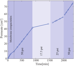
We have run several simulations with different values of w. The grid resolution is $10000\times 20$, corresponding to a flake length of $10^{-6}\;m$ , which we take as a representative experimental value, Amadei et al. (2016). The mesoscale model was tested against experimental measurements of permeability. The permeability of the membrane is defined as $\kappa=\mu u_{s}/|\nabla p|$, where $\mu$ is the dynamic viscosity, $\nabla p$ the pressure gradient across the membrane and $u_{s}$ the superficial velocity defined as the ratio between the membrane discharge per unit area. It is worth recalling that in the Darcy regime, the permeability $\kappa$ is pressure independent (see figure S 5 in the supporting information). In order to test our numerical results against experimental data, we inferred the experimental values of flow rates (mass flow per unit time) from the permeate vs time plot, reported in Fig. 2, for different values of the applied pressure. From these data, we compute a dimensionless permeability $\kappa^{*}=\kappa/(2h)^{2}$, where $2h$ represents the spacing between two GO layers. X-ray diffraction measurements give $2h\sim\;0.8nm$. The experimental value of the dimensionless permeability $\kappa^{*}$ for a $\sim 30\;nm$ thick membrane of diameter $d=2\;cm$ is $\kappa^{*}\sim 2.8\times 10^{-4}$, corresponding to a permeability of $3.6\pm 0.5\;LMH/bar$. This value of permeability is in line with data previously reported for ultrathin ($<50\;nm$) GO membranes ( see Han et al. (2013); Kovtyukhova et al. (1999); Hu and Mi (2013)) and represents a promising result for nanofiltration applications. It is important to underline that higher values of permeability have been achieved for GO membranes. However, these values can be connected to the presence of defects or larger GO nanochannels due to the chemical modification of the GO membranes Han et al. (2013); Xia et al. (2015); Ying et al. (2014). Higher permeability can also be achieved by intercalating the GO membranes with high aspect ratio nanoarchitectures, such as CNT Huang et al. (2013); Goh et al. (2015).

Figure 3: Left panel: Solid lines with symbols represent the simulated permeabilities (truncated ($\kappa_{h}$) and non-truncated ($\kappa_{\text{w}}$)) while black dashed line reports the average experimental ($\kappa_{exp}$) value as a function of w$=0.1$, $0.2$, $0.3$, $0.4\;nm$ and $h=0.4\;nm$. Right panel: solid lines with symbols represent the slip length computed with the LB approach (truncated ($L_{s,w}$) and non-truncated ($L_{s,h}$)) while the dashed line stands for the NEMD average slip length Wei et al. (2014a). In both figures grey shaded area identifies the the error bars of the experimental permeability and of the NEMD slip lengths. The case w$=0$ correspond to free-slip conditions, taken as representative of the FWT consitions (see the main text).

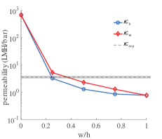
Fig. 3 illustrates two comparisons, for both the truncated and non-truncated Langevin frictions: i) between the permeability obtained by mesoscopic simulations and experiments; ii) between the slip length obtained by NEMD Wei et al. (2014a) and by this study. The case w$=0$ corresponds to a simulation without the Langevin friction, i.e. pure free-slip hydrodynamics. By free-slip we mean boundary conditions which leave the flow momentum tangential to the wall unchanged. This is representative of the FWT regime observed in pristine graphene experiments. Note that the flow still reaches a steady-state solution on account of the localized dissipation experienced at the sharp $90^{\circ}$ turns between two subsequent layers, visible in Fig. 1c. The main outcome from Fig. 3 is a dramatic drop in permeability of two orders of magnitude, already at w$=0.1\;nm$, i.e. w$/h=0.25$. Such a dramatic drop in permeability is consistent with experimental observations that report a suppression of FWT regimes in the presence of hydroxyl groups. Further increments of w lead to a sizable reduction in permeability by circa one order of magnitude, from w$=0.1\;nm$ to w$=0.4\;nm$. It is worth noting that, the employed resolution ($\Delta x=0.1\;nm$) poses a constraint on the lower bound of w. We note that the truncated ($\kappa_{\text{w}}$, $\delta=\text{w}$) and non-truncated ($\kappa_{h}$, $\delta=h$) scenarios yield nearly the same picture with only minor quantitative variations. Moreover, Fig. 3 shows that for both the truncated and non-truncated scenario, the slip length remains between $0.5\;nm$ and $2\;nm$, in agreement with the values provided by NEMD Wei et al. (2014a). It is worth noting that the best match of the experimental (permeability) and NEMD (slip lengths) results with the simulations is obtained when w is between $0.1\;nm$ and $0.2\;nm$ (i.e. w$/h=0.25\div 0.5$), which agrees with the physical dimension of the oxygen functionalities in the GO nanochannels Haynes (2014). This further corroborates the validity of the model and its potential to capture the physical phenomena in 2D nanostructured inspired materials within an efficient computational framework.

Inside the flow structure. Next, we proceed to inspect the internal structure of the flow. In particular, we focus on the occurrence of slip flow in the presence of hydroxyl, as recently observed in non-equilibrium molecular dynamics simulations Wei et al. (2014a). As previously discussed, slip flow is a typical manifestation of individual non-hydrodynamic behavior driven by non-equilibrium effects near the wall. To glean quantitative insights into such non-equilibrium phenomena is informative for inspecting the one-dimensional cross-flow profiles $u_{x}(y)$ for different values of w versus the case of free-slip boundary conditions.

Figure 4: (a) Flow profiles $u_{x}(y)$ for different values of the friction length w and cutoff length $\delta$, $(\text{w},\delta)$. The horizontal line refers to the free-slip flow in the absence of Langevin friction. The two numbers within parenthesis denote the values of w and $\delta$. Friction and cutoff lengths are made dimensionless by dividing them by half of the channel spacing $h=0.4\;nm$. In panel (b) we report the velocity profile obtained by the Langevin-LB on a $3\;nm$ wide channel flow using $50$ lattice point compared to the MD profile taken from Huang et al. (2013).On the $x$-axis the non-dimensional channel width ($\text{y}/2h$) is reported. The profiles are rescaled by the peak value of the velocity.

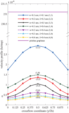
Fig. 4a illustrates that the flow profiles display a Poiseuille-like parabolic trend in the bulk region, smoothly turning into a flat profile near the wall, with a positive curvature and a small non-zero slip velocity. The comparison between the pristine graphene profile with the other profiles highlights the major drop of mass flow due to Langevin friction. The increase of w leads to the suppression and flattening of the water profiles. From the velocity profiles, we compute the slip length according to $L_{s}=\lim_{y\to 0}\;|\frac{u_{x}(y)}{\partial_{y}u_{x}(y)}|$. As previously discussed for Fig. 3, we confirm the presence of a residual slip length, which is small in absolute physical units, but fairly sizable in units of the channel width $h$, namely $L_{s}/2h\sim 0.5$. Furthermore, the effect of the different cut-off lengths employed in the truncated $(\delta=\text{w})$ and non-truncated $(\delta=h)$ Langevin is minor, leading to slight differences in both the membrane permeability and slip lengths. To further test the robustness of this approach in Fig. 4(b) we report a comparison between the velocity profiles obtained by the Langevin-LB and the MD approach Huang et al. (2013) for a $3\;nm$ wide GO channel, showing an outstanding agreement between the two models.

We conclude this Letter with an ex-post analysis of our mesoscale model in light of the numerical results discussed above. First, we note that although both friction and viscous dissipation withstand the driving action of the pressure gradient, they operate according to very different and competing mechanisms. Friction drives the fluid towards the following local flow configuration:

$$u_{x}^{(L)}(y)=\frac{|\nabla_{x}p|}{\rho\gamma(y)}$$ (4)

This results in a slip-flow $u_{slip}=|\nabla_{x}p|/(\rho\gamma_{0})$ (independent of w) at the wall and the corresponding slip length is $L_{s}=$w. Viscous dissipation, on the other hand, drives the fluid towards a parabolic Hagen-Poiseuille profile,

$$u_{x}^{(H)}(y)=u_{H}[\;\frac{y}{h}(2-\frac{y}{h})+Const.].$$ (5)

where we have set $u_{H}=\frac{\nabla_{x}p}{\rho\nu/h^{2}}$. The above hydrodynamic solution is compatible with either slip or non-slip flow conditions, depending on the value of the constant at the right hand side. In slip-hydrodynamics $Const.=L_{s}/h$, so that $L_{s}/h\to 0$ recovers standard no-slip hydrodynamics. This value can only be prescribed a-priori, exposing the weakness of the hydrodynamic approach previously mentioned.

The two profiles, $u_{x}^{(L)}(y)$ and $u_{x}^{(H)}(y)$ cannot coexist other than in an intermediate compromising form, resulting from the smoothing of the Langevin profile due to viscous dissipation. To gain a deeper understanding, in Fig. 5 we report the friction and viscous forces separately, for the case w$=\delta=0.2\;nm$.

Figure 5: Friction and viscous dissipation forces (in lattice units) as a function of the crossflow coordinate $y/2h$ for the case w$=0.2\;nm$, $\delta=0.2\;nm$. For the sake of reference, the corresponding (rescaled) flow profile is also reported.

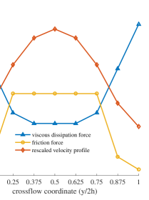
As one can see, the bulk flow is dominated by viscous dissipation (friction is zero in the bulk because $\delta=0.2\;nm$), while in the vicinity of the wall, friction takes over. However, the two contributions become comparable but opposite in sign due to the positive curvature of the flow profile. We have also checked through separate simulations that the sign inversion of hydrodynamic dissipation holds true at higher resolution (see Fig. 4(b)). The inversion of the dissipative force, namely $F_{d}=\rho\nu\frac{\partial^{2}u}{\partial y^{2}}>0$ at the wall is a genuine effect of the spatially distributed decaying Langevin friction. Indeed, since the free-slip boundary condition forces $\nu\frac{\partial^{2}u}{\partial y^{2}}=0$, the near-wall dissipative force is dominated by the Langevin friction, which is incompatible with $F_{d}=0$. Since Langevin friction decays exponentially away from the wall, the near-wall flow profile must grow exponentially according to eq.4, thus exhibiting the observed inverted (positive) curvature. Because of the exponential decay of the extended friction, the bulk region is still dominated by viscous dissipation, as reflected by the bulk parabolic profile clearly visible in fig.5. The onset of the inverted curvature is a distinctive signature of the coexistence between single particle Langevin friction (slip-flow) and collective hydrodynamics (bulk flow). Differently from continuum methods, which impose the slip length through the boundary conditions, in our model it naturally emerges from the self-consistent competition between extended friction and hydrodynamic dissipation. This extra-freedom is key to recover the inverted curvature profile.

Conclusions. In summary, our numerical simulations portray the following picture. Even a small amount of spatially extended Langevin friction, w$/h=0.25$, leads to a dramatic drop in the mass flow compared to free-slip hydrodynamics. Such friction still supports a small residual slip-flow at the wall, with a slip length of the order of the friction length w. However, this flow is largely negligible compared to the free-slip in the absence of Langevin friction. The net result is a dramatic loss of permeability due to the presence of the functional groups, hence the inhibition of the FWT regime observed in pristine graphene membranes. Viscous effects dominate the bulk flow and contribute to the smoothing of the sharp features of the flow due to the presence of the hydroxyl and epoxy. Inspection of the flow structure reveals an inverted curvature in the near-wall region, which connects smoothly with a parabolic profile in the bulk region Such inverted curvature is a distinctive signature of the coexistence between single particle Langevin friction and collective hydrodynamics.

I Supporting Information

I.1 Hummers’ Method

GO solution was prepared using a modified Hummers’ method with additional pre-oxidation of the graphite flakes. $5g$ of the graphite powder were pre-oxidized using sulfuric acid ($30mL$; $97$$\%$ $H_{2}SO_{4}$), phosphorus pentoxide ($4.2g$; $P_{2}O_{5}$), and potassium persulfate ($4.2g$; $K_{2}S_{2}O_{8}$) in a water bath at $75^{\circ}C$ for $4.5h$. The mixture was then cooled to room temperature and diluted with $700mL$ of deionized water (DI) and vacuum filtered through a poly(tetrafluoroethylene) membrane (pore size $5\mu m$). After pre-oxidation, the modified Hummers’ method was carried out by suspending the pre-oxidized material in $H_{2}SO_{4}$ ($150mL$; $97$$\%$) in an ice bath for $20min$. Potassium permanganate was slowly added ($15g$; $KMnO_{4}$) and the solution was heated to $35\circ C$ for $2h$. The process was completed by adding $250mL$ of DI water and heating the mixture to $70^{\circ}C$ for an additional $2h$. The reaction was quenched with hydrogen peroxide ($30mL$; $H_{2}O_{2}$) and DI water ($750mL$). In order to quench the unreacted reagent and clean the solution, the product was then filtered through a $300\mu m$ testing sieve, then through glass fiber and centrifuged for $1h$ at $5000RPM$ (Sorvall RC-5C plus). The supernatant was discared whereas the precipitate was washed with hydrochloric acid ($400mL$, $10$$\%$ $HCl$). The sieving, centrifugation, and washing process was then repeated using DI (two times) and ethanol ($EtOH$, two times). The final solution was then dispersed in $300mL$ of $EtOH$ at a concentration of $\simeq 0.1mg/L$. The overall yield of the process was circa $5$$\%$. Figure S 6 represents a SEM image of a drop casted GO solution on a silicon wafer. As one can see, more than $90$ $\%$ of the GO flakes is monolayer with an average area of $1.5\pm 0.4\mu m^{2}$.

Figure 6: monolayer GO flake’s on a silica wafer.

I.2 Membrane characterization

Figure S 7 represents SEM images obtained after depositing $2nm$ $Pt/Pd$ layer onto the membranes via an EMS300R sputter coater. Figure S 7a shows the bare PVDF membrane characterized by pores size of $\simeq 200nm$. Figure S 7b represents the PVDF membrane after the GO deposition via vacuum filtration.

Figure 7: SEM characterization of (a) bare PVDF membrane, (b) GO membrane on PVDF and (c) cross section of GO membrane.

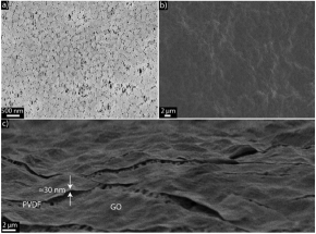
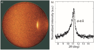
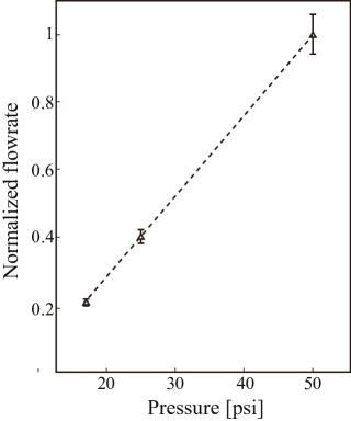
Figure S 7c shows a cross section of the membrane, which highlights the extreme thinness of the GO layer (circa $30nm$). It is also possible to observe that the GO layer conserves the morphology of the underneath PVDF membrane. As explained in the main text, the XRD spectra was obtained by integrating a 2D diffraction pattern image (Fig. S 8a). The XRD spectra (Fig. S 8b) displays a distinct peak centered at $11.1^{\circ}$. By using Bragg’s law, this value can be converted to $0.8nm$, which represents the spacing between the GO flakes. The permeability tests were carried out with a custom-made dead-end filtration system (Figure S 9). The filtration system includes a $3L$ reservoir (e.g. pressure pot). The pressure was regulated with a pressure gauge from Ingersoll and the GO membrane was placed inside a stainless steel EDM Millipore filter holder. Finally. fig. S 10 displays the normalized flowrate versus applied pressure for the GO membrane. As mentioned in the main text, the permeability is independent from the applied pressure and this is testified by the linear fitting.

Figure 8: (a) 2 d image of the Go membrane. (b) XRD characterization of GO membrane showing a peak centered at $11.1^{\circ}$.

Figure 9: Dead end filtration system.

I.3 Some remarks on the slip length in nano-channel flows

The possibility of slip flow was contemplated by Navier himself as early as in 1823, by postulating a direct proportionality between the slip velocity and the gradient of the velocity at the wall. For a one-dimensional flow across parallel plates at a distance $h$, the Navier slip-boundary adds a slip term $L_{s}/h$, on top of the parabolic Poiseuille bulk profile $1-(y/h)^{2}$. One may therefore argue that the notion of slip-flow is perfectly compatible with continuum hydrodynamics. This is certainly true for the case of macroscopic flows, in which the slip term $L_{s}/h\ll 1$. However, for nanoflows, where $h$ becomes comparable with $L_{s}$, this is no longer true, because the slip term becomes dominant over the bulk one. Moreover, under such conditions, it is not obvious that the bulk component still obeys a parabolic flow profile, because $L_{s}/h\sim 1$ means that non- equilibrium is as strong as equilibrium, thus contradicting the low-Knudsen assumption, $L_{s}/h\ll 1$, which lies at the basis of the continuum picture.

Figure 10: Flowrate versus Pressure plot. The linear trend clearly denotes a Darcy behaviour of the GO membrane.