Second Order Cone Constrained Convex Relaxations for Nonconvex Quadratically Constrained Quadratic Programming

Abstract

In this paper, we present new convex relaxations for nonconvex quadratically constrained quadratic programming (QCQP) problems. While recent research has focused on strengthening convex relaxations using reformulation-linearization technique (RLT), the state-of-the-art methods lose their effectiveness when dealing with (multiple) nonconvex quadratic constraints in QCQP. In this research, we decompose and relax each nonconvex constraint to two second order cone (SOC) constraints and then linearize the products of the SOC constraints and linear constraints to construct some effective new valid constraints. Moreover, we extend the reach of the RLT-like techniques for almost all different types of constraint-pairs (including valid inequalities by linearizing the product of a pair of SOC constraints, and the Hadamard product or the Kronecker product of two respective valid linear matrix inequalities), examine dominance relationships among different valid inequalities, and explore almost all possibilities of gaining benefits from generating valid constraints. Especially, we successfully demonstrate that applying RLT-like techniques to additional redundant linear constraints could reduce the relaxation gap significantly. We demonstrate the efficiency of our results with numerical experiments.

1 Introduction.

We consider in this paper the following class of quadratically constrained quadratic programming (QCQP) problems:

$$\rm{(P)}~{}~{}~{} ~{}\min x^{T}Q_{0}x+c_{0}^{T}x$$

$$~{}\rm{s.t.} x^{T}Q_{i}x+c_{i}^{T}x+d_{i}\leq 0,~{}i=1,\ldots,l,$$

$$a_{j}^{T}x\leq b_{j},~{}j=1,\ldots,m,$$

where $Q_{i}$ is an $n\times n$ symmetric matrix, $c_{i}\in\Re^{n}$, $i=0\ldots,l$, $d_{i}\in\Re$, $i=1\ldots,l$ and $a_{j}\in\Re^{n},~{}b_{j}\in\Re$, $j=1,\ldots,m$. Without loss of generality, we assume that $Q_{i}$ is not a zero matrix for $i=1,\ldots,l$. We further partition the quadratic constraints into the following two groups:

$$\mathcal{C} =\{i:~{}Q_{i}\text{ is positive semidefinite},~{}i=1,\ldots,l\},$$

$$\mathcal{N} =\{i:~{}Q_{i}\text{ is not positive semidefinite},~{}i=1,\ldots,l\}.$$

Without loss of generality, we assume in this paper the cardinality of $\mathcal{C}$ is $k$ ($k\leq l$). QCQP problems arise in various areas, for example, combinatorial optimization, portfolio selection problems, economic equilibria, 0–1 integer programming and various applications in engineering. In the past few decades, QCQP has been widely investigated in the literature (see, e.g., [2, 8, 28, 6, 15, 19, 20, 30, 31]), due to its elegance in formulation and a wide spectra of applications.

QCQP in general is NP-har [23], even when it only has linear constraints [21], although some special cases of QCQP are polynomially solvable [4, 5, 10, 27, 7]. As a global optimal solution of QCQP is generally hard to compute due to its NP-hardness, based on various kinds of relaxations, branch and bound methods have been developed in the literature to find exact solutions for QCQP problems; see, e.g., [20, 12]. It is well known that the efficiency of a branch and bound method depends on two major factors: the quality of the relaxation bound and its associated computational cost. Recent decades have witnessed an increasing attention on constructing convex relaxations enhanced with various valid inequalities. The survey paper [6] compared the computational speed and quality of the gaps of various semidefinite programming (SDP) relaxations with different valid inequalities for QCQP problems. Sherali and Adams [24] first introduced the concept of “reformulation-linearization technique” (RLT) to achieve a lower bound of problem (P). Anstreicher in [1] proposed a theoretical analysis for successfully applying RLT constraints to remove a large portion of the feasible region for the relaxation, and suggested that a combination of SDP and RLT constraints leads to a tighter bound. This standpoint holds true for the relaxations with all other valid inequalities based on the idea behind RLT in this paper. Sturm and Zhang [27] developed the so-called SOC-RLT constraints (or called rank-2 second-order inequalities in [29, 31]) to solve the problem of minimizing a quadratic objective function subject to a convex quadratic constraint and a linear constraint exactly when combined with its SDP relaxation. More specifically, they rewrote a convex quadratic constraint as a second order cone (SOC) constraint and linearized the product of the SOC and linear constraints. Burer and Saxena [11] discussed how to utilize the SOC-RLT constraints to get a tighter bound than the SDP+RLT relaxation for general mixed integer QCQP problems. Recently, Burer and Yang [13] demonstrated that the SDP+RLT+(SOC-RLT) relaxation has no gap in an extended trust region problem of minimizing a quadratic function subject to a unit ball and multiple linear constraints, where the linear constraints do not intersect with each other in the interior of the ball.

However, all methods mentioned above lose their effectiveness when dealing with (multiple) nonconvex quadratic constraints in QCQP problems. The state-of-the-art in dealing with nonconvex quadratic constraints is to directly lift the quadratic terms as the basic SDP relaxation does. This recognition and the success of combining SDP relaxations with RLT and SOC-RLT constraints (for convex quadratic constraints) motivate our study in this paper. Using the basic ideas behind SOC-RLT constraints, our method constructs valid inequalities based on linearizing the product of the nonconvex quadratic constraints and linear constraints, and performs better than the state-of-the-art convex relaxations for problem (P). We call our newly developed valid inequalities Generalized SOC-RLT (GSRT) constraints. For simplicity of analysis, we call any nonconvex quadratic constraint type-A and a nonconvex quadratic constraint $x^{T}Q_{i}x+c_{i}^{T}x+d_{i}\leq 0$ type-B if $c_{i}\in{\rm Range}(Q_{i})$. Although this range condition for type-B could be numerically hard to check in general, it can be readily verified in some special cases, e.g., $Q_{i}$ is nonsingular or $c_{i}\in{\rm Range}(Q_{i})$ is known to hold in advance for some specific problem data set. To construct GSRT constraints, we first introduce a new augmented variable $z_{i}$ corresponding to each nonconvex constraint $x^{T}Q_{i}x+c_{i}^{T}x+d_{i}\leq 0,~{}i\in\mathcal{N},$ and then decompose the matrix $Q_{i}$ according to the signs of its eigenvalues such that $Q_{i}=L_{i}^{T}L_{i}-M_{i}^{T}M_{i}$. Depending on different techniques in handling the linear term, the decomposition of $x^{T}Q_{i}x+c_{i}^{T}x+d_{i}\leq 0$ further results in two types of GSRT, i.e., type-A GSRT constraint (GSRT-A) and type-B GSRT constraint (GSRT-B) as follows. GSRT-A is derived from the equivalence between $x^{T}Q_{i}x+c_{i}^{T}x+d_{i}\leq 0$ and the following two constraints,

$$\left\lVert\left.\left(\begin{array}[]{c}L_{i}x\\ \frac{1}{2}(c_{i}^{T}x+d_{i}+1)\end{array}\right)\right.\right\rVert\leq z_{i},$$ (3)

$$\left\lVert\left(\begin{array}[]{c}M_{i}x\\ \frac{1}{2}(c_{i}^{T}x+d_{i}-1)\end{array}\right)\right\rVert=z_{i},$$ (6)

where the equivalence is easily derived by substituting (6) into (3). If a type-B quadratic constraint holds for index $i$ with $c_{i}\in{\rm Range}(Q_{i})$, GSRT-B constraints are then constructed by decomposing $x^{T}Q_{i}x+c_{i}^{T}x+d_{i}\leq 0$ in one of the following two different ways:

• i) if $\frac{1}{4}(c_{i}^{T}Q_{i}^{\dagger}c_{i})-d_{i}\geq 0$, we decompose $x^{T}Q_{i}x+c_{i}^{T}x+d_{i}\leq 0$ as

  $$\left.\begin{array}[]{l}\left\lVert L_{i}(x+x_{0})\right\rVert\leq z_{i},\\ \left\lVert\left(\begin{array}[]{c}M_{i}(x+x_{0})\\ \Delta\end{array}\right)\right\rVert=z_{i},\end{array}\right.$$ (11)

  where $\Delta=\sqrt{\frac{1}{4}(c_{i}^{T}Q_{i}^{\dagger}c_{i})-d_{i}}$, $x_{0}=\frac{1}{2}Q_{i}^{\dagger}c_{i}$ and $A^{\dagger}$ denotes the Moore–Penrose pseudoinverse for matrix $A$.

• ii) if $\frac{1}{4}(c_{i}^{T}Q_{i}^{\dagger}c_{i})-d_{i}<0$, we decompose $x^{T}Q_{i}x+c_{i}^{T}x+d_{i}\leq 0$ as

  $$\left.\begin{array}[]{l}\left\lVert\left(\begin{array}[]{c}L_{i}(x+x_{0})\\ \Delta\end{array}\right)\right\rVert\leq z_{i},\\ \left\lVert M_{i}(x+x_{0})\right\rVert=z_{i},\end{array}\right.$$ (16)

  where $\Delta=\sqrt{d_{i}-\frac{1}{4}(c_{i}^{T}Q_{i}^{\dagger}c_{i})}$, $x_{0}=\frac{1}{2}Q_{i}^{\dagger}c_{i}$.

Since the equality constraint (6) is nonconvex and intractable, we relax (6) to an inequality to obtain an SOC constraint (which is convex and tractable),

$$\left\lVert\left(\begin{array}[]{c}M_{i}x\\ \frac{1}{2}(c_{i}^{T}x+d_{i}-1)\end{array}\right)\right\rVert\leq z_{i}.$$ (17)

Multiplying any linear constraint to both sides of the above two kinds of SOC constraints in (3) and (17), respectively, and linearizing the products lead to additional valid inequalities. Moreover, we construct valid equalities by linearizing the squared form of (6), i.e., linearizing the following equality,

$$xM_{i}^{T}M_{i}x+\frac{1}{4}(c_{i}^{T}x+d_{i}-1)^{2}=z_{i}^{2}.$$ (18)

The GSRT-A constraints consist of SOC constraints in (3) and (17), the linearization of the products of SOC constraints in (3) and (17) with any original linear constraint, and the linearization of (18). With similar techniques, we can construct GSRT-B constraints according to the different decomposition schemes of $x^{T}Q_{i}x+c_{i}^{T}x+d_{i}\leq 0$, given in (11) and (16), respectively. Note that GSRT-A constraints can be generated from any pair of a nonconvex quadratic constraint and a linear constraint, but GSRT-B constraints can only be generated from those pairs under the range condition $c_{i}\in{\rm Range}(Q_{i})$. That is, we can always construct GSRT-A, but have limited ability to construct GSRT-B only under the range condition $c_{i}\in{\rm Range}(Q_{i})$. We then prove that the GSRT relaxation, which stands for the SDP relaxation enhanced with RLT, SOC-RLT and GSRT constraints, achieves a much tighter lower bound for problem (P) than the sate-of-the-art relaxation in the literature.

Another RLT-based technique in the literature is to introduce and attach additional redundant linear constraints to the original QCQP problem and then apply the RLT and SOC-RLT techniques. Zheng et al. [31] proposed a decomposition-approximation method for generating convex relaxations to get a tighter lower bound than the SDP+RLT+(SOC-RLT) bound. Enlightened by the decomposition-approximation method in [31], we introduce a new relaxation by generating extra RLT, SOC-RLT and GSRT constraints with extra redundant linear inequalities. We further demonstrate that this relaxation dominates the decomposition-approximation method in [31] for problem (P) with an extra nonnegativity constraint $x\geq 0$.

Inspired by the GSRT constraints, we also explore and construct a new class of valid inequalities by linearizing the product of any pair of SOC constraints, termed SOC-SOC-RLT (SST) constraint. Moreover, we demonstrate that this new class of valid inequalities is equivalent to a valid linear matrix inequality (LMI) formed by a submatrix of the Kronecker product constraint proposed in [3], termed Kronecker SOC-RLT (KSOC) constraint. However, as the KSOC constraint is a large-scale LMI, its dimensionality may prevent its direct application from practical implementation. We thus discuss the tradeoff between using KSOC and its submatrices with respect to the bound quality and computational costs. We also investigate several other KSOC constraints and their dominance relationship with the valid inequalities discussed in this paper.

We illustrate below the different kinds of valid inequalities generated by RLT-like technique, i.e., linearizing the product of the left hand side yields the valid inequalities on the right hand side, and also indicate in the list the sections (or subsections) in which different RLT-like techniques are developed,

$$\begin{array}[]{rcll}\rm L\times L&\Longrightarrow&\rm RLT~{}([22])&\text{Section 2.1,}\\ \rm SOC(convex)\times L&\Longrightarrow&\rm SOC\mbox{-}RLT~{}([25])&\text{Section 2.1,}\\ \rm SOC(nonconvex)\times L&\Longrightarrow&\rm GSRT&\text{Section 2.2,}\\ \rm M(\succeq 0)\circ M(\succeq 0)&\Longrightarrow&\rm HSOC~{}([29]){}{}{}{}{}{}&\text{Section 3,}\\ \rm SOC\times SOC&\Longrightarrow&\rm SST{}{}{}{}{}{}{}{}{}{}{}{}{}{}{}{}{}&\text{Section 4,}\\ \rm M(\succeq 0)\otimes M(\succeq 0)&\Longrightarrow&\rm KSOC(\succeq 0)~{}([3]\text{ and this paper}){}&\text{Section 5,}\end{array}$$

where $\rm L$ represents a linear inequality constraint, $\rm SOC(convex)$ ($\rm SOC(nonconvex)$, respectively) represents an SOC constraint generated from a convex (nonconvex, respectively) constraint, $\rm M(\succeq 0)$ represents an LMI, HSOC represents the valid inequalities generated by linearizing the Hadamard product of two valid LMIs (expressed in (77) later in the paper) in [31] and KSOC represents the valid inequalities generated by linearizing the Kronecker product of two valid LMIs first derived in [3].

In general, there is no dominance relationship among the valid inequalities RLT, SOC-RLT, GSRT and KSOC. Furthermore, although SST, HSOC and the valid LMI given in (106) later in the paper are not dominated by RLT, SOC-RLT and GSRT, they are all dominated by a KSOC valid inequality as we will prove in Section 5. When a new valid inequality has no dominance relationship with the existing constraints in the formulation, adding this additional valid inequality to the constraints should yield a tighter relaxation. So the guiding principle of our research is to extend the RLT-like technique to derive effective valid inequalities to strengthen the SDP relaxation, especially to develop effective valid inequalities from nonconvex quadratic constraints.

We summarize now the main contributions of this paper in the following three aspects.

• We derive the GSRT constraints, which represent the first attempt in the literature to construct new valid inequalities for nonconvex quadratic constraints using RLT-like techniques.

• We extend the reach of the RLT-like techniques for almost all different types of constraint-pairs and explore almost all possibilities of gaining benefits from generating valid constraints. We also successfully demonstrate that applying RLT-like techniques to additional redundant linear constraints could reduce the relaxation gap.

• We examine possible dominance relationships among different valid inequalities generated from various RLT-like techniques. We also discuss the tradeoff between the tightness of the bound and the computational cost.

The rest of the paper is organized as follows. In Section 2, we first review existing convex relaxations with various valid inequalities in the literature and then propose our novel GSRT constraints. In Section 3, we apply RLT-like techniques to additional redundant linear constraint and demonstrate a dominance relationship of our method over the method in [31]. We propose in Section 4 another class of valid inequalities, SST constraints, by linearizing the product of two SOC constraints. In Section 5, we introduce KSOC constraints in the recent literature and show their relationships with the previous constraints discussed in the paper. After we demonstrate good performance of GSRT from numerical tests in Section 6, we offer our concluding remarks in Section 7.

Notation We use $v(\cdot)$ to denote the optimal value of problem $(\cdot)$. Let $\left\lVert x\right\rVert$ denote the Euclidean norm of $x$, i.e., $\left\lVert x\right\rVert=\sqrt{x^{T}x}$, and $\left\lVert A\right\rVert_{F}$ denote the Frobenius norm of a matrix $A$, i.e., $\left\lVert A\right\rVert_{F}=\sqrt{tr(A^{T}A)}$. The notation $A\succeq 0$ refers that matrix $A$ is positive semidefinite and the notation $A\succeq B$ implies that $A-B\succeq 0$. The inner product of two symmetric matrices is defined by $A\cdot B=\sum_{i,j=1,\ldots,n}A_{ij}B_{ij}$, where $A_{ij}$ and $B_{ij}$ are the $(i,j)$ entries of $A$ and $B$, respectively. We also use $A_{i,\cdot}$ and $A_{\cdot,i}$ to denote the $i$th row and column of matrix $A$, respectively. Notation ${\rm rank}(A)$ denotes the rank of matrix $A$. We use ${\rm diag}(v)$, where $v$ is a column vector, to denote a diagonal matrix with its $i$th diagonal entry being $v_{i}$ and ${\rm Diag}(A)$ to denote the column vector with its $i$th entry being $A_{ii}$. For a positive semidefinite matrix $A$ with spectral decomposition $A=U^{T}DU$, where $D$ is a diagonal matrix, we use notation $A^{\frac{1}{2}}$ to denote $U^{T}D^{\frac{1}{2}}U$, where $D^{\frac{1}{2}}$ is a diagonal matrix with $\sqrt{D_{ii}}$ being its $i$th entry.

2 Generalized SOC-RLT constraints

In this section, we first present the basic SDP relaxation for problem (P) and its strengthened variants with RLT and SOC-RLT constraints in the literature and then propose the new GSRT constraints.

2.1 Preliminary

Let us now first review some existing relaxations for problem $\rm(P)$ in the literature. By lifting $x$ to matrix $X=xx^{T}$ and relaxing $X=xx^{T}$ to $X\succeq xx^{T}$, which is further equivalent to $\left(\begin{array}[]{cc}1&x^{T}\\ x&X\end{array}\right)\succeq 0$ due to the Schur complement, we have the following basic SDP relaxation for problem (P):

$${\rm(SDP)} ~{}\min Q_{0}\cdot X+c_{0}^{T}x$$ (19)

s.t. $$Q_{i}\cdot X+c_{i}^{T}x+d_{i}\leq 0,~{}i=1,\ldots,l,$$

$$a_{j}^{T}x\leq b_{j},~{}j=1,\ldots,m,$$ (20)

$$\left(\begin{array}[]{cc}1&x^{T}\\ x&X\end{array}\right)\succeq 0,$$ (23)

where $Q_{i}\cdot X={\rm trace}(Q_{i}X)$ is the inner product of matrices $Q_{i}$ and $X$. Note that the Lagrangian dual problem of problem (P) is

$$\rm(L)~{} \max \tau$$

$$\rm s.t. \left(\begin{array}[]{cc}Q_{0}&\frac{c_{0}}{2}\\ \frac{c_{0}^{T}}{2}&-\tau\end{array}\right)-\sum_{i}^{l}\lambda_{i}\left(\begin{array}[]{cc}Q_{i}&\frac{c_{i}}{2}\\ \frac{c_{i}^{T}}{2}&d_{i}\end{array}\right)-\sum_{i}^{m}\mu_{j}\left(\begin{array}[]{cc}0&\frac{a_{j}}{2}\\ \frac{a_{j}^{T}}{2}&-b_{j}\end{array}\right)\succeq 0,$$

$$\lambda_{i}\geq 0,~{}i=1,\ldots,l,~{}\mu_{j}\geq 0,~{}j=1,\ldots,m,$$

which is also known as the Shor’s relaxation [26]. It is well known (see, e.g., [9]) that (L) is the conic dual of (SDP) and (SDP) and (L) have the same optimal value when the strong duality holds for (SDP). Furthermore, the strong duality holds for (SDP) when (SDP) is bounded from below and Slater condition holds for (SDP). When the Slater condition holds true for problem (P), i.e., there exists a strictly feasible solution $\hat{x}$ such that $\hat{x}^{T}Q_{i}\hat{x}+c_{i}^{T}\hat{x}+d_{i}<0,~{}i=1,\ldots,l$ and $a_{j}^{T}\hat{x}\leq b_{j},~{}j=1,\ldots,m$, the Slater condition for (SDP) automatically holds, e.g., by letting $\hat{X}=\hat{x}\hat{x}^{T}+\epsilon I$, for sufficiently small $\epsilon>0$ such that $Q_{i}\cdot\hat{X}+c_{i}^{T}\hat{x}+d_{i}\leq x^{T}Q_{i}\hat{x}+c_{i}^{T}\hat{x}+d_{i}+\epsilon\lambda_{max}(Q_{i})<0$, where $\lambda_{max}(Q_{i})$ is the maximum eigenvalue of matrix $Q_{i}$.

As the basic SDP relaxation is often too loose, valid inequalities have been considered to strengthen $\rm(SDP)$ in the literature. One widely used technique in strengthening the basic SDP relaxation is the RLT [24], which linearizes the product of any pair of linear constraints, i.e.,

$$(b_{i}-a_{i}^{T}x)(b_{j}-a_{j}^{T}x)=b_{i}b_{j}-(b_{j}a_{i}^{T}+b_{i}a_{j}^{T})x+a_{i}^{T}xx^{T}a_{j}\geq 0.$$

By linearizing $xx^{T}$ to $X$, we get a tighter (SDP) relaxation enhanced with the RLT constraints for problem (P):

$${\rm(SDP_{RLT})} ~{}\min Q_{0}\cdot X+c_{0}^{T}x$$ (25)

s.t. $$(\ref{QC}),(\ref{LC}),(\ref{SDP}),$$

$$a_{i}a_{j}^{T}\cdot X+b_{i}b_{j}-b_{j}a_{i}^{T}x-b_{i}a_{j}^{T}x\geq 0,~{}\forall 1\leq i<j\leq m.$$

Note that when $i=j$, the RLT constraint $a_{i}a_{j}^{T}\cdot X+b_{i}b_{j}-b_{j}a_{i}^{T}x-b_{i}a_{j}^{T}x\geq 0$ is dominated by (23) and can be omitted.

Moreover, it has been shown in [11] and [27] that SOC-RLT constraints can be used to strengthen the convex relaxation $\rm(SDP_{RLT})$ for problem (P). In particular, decomposing a positive semidefinite matrix $Q_{i}$ as $Q_{i}=B_{i}^{T}B_{i}$, $i\in\mathcal{C}$, we can rewrite the convex quadratic constraint in an SOC form, i.e.,

$$\left.\begin{array}[]{l}x^{T}Q_{i}x\leq-d_{i}-c_{i}^{T}x\Rightarrow-d_{i}-c_{i}^{T}x\geq 0\\ x^{T}Q_{i}x\leq-d_{i}-c_{i}^{T}x\end{array}\right\}\Rightarrow$$ (28)

$$\left\lVert\left(\begin{array}[]{c}B_{i}x\\ \frac{1}{2}(-d_{i}-c_{i}^{T}x-1)\end{array}\right)\right\rVert\leq\frac{1}{2}(-d_{i}-c_{i}^{T}x+1).$$ (31)

Multiplying the linear term $b_{j}-a_{j}^{T}x\geq 0$ to both sides of the above SOC yields the following valid inequality,

$$(b_{j}-a_{j}^{T}x)\left(\left\lVert\left(\begin{array}[]{c}B_{i}x\\ \frac{1}{2}(1+d_{i}+c_{i}^{T}x)\end{array}\right)\right\rVert\right)\leq\frac{1}{2}(b_{j}-a_{j}^{T}x)(1-d_{i}-c_{i}^{T}x),$$

whose linearization becomes the following SOC-RLT constraint,

$$\begin{array}[]{ll}&\left\lVert\begin{pmatrix}B_{i}(b_{j}x-Xa_{j})\\ \frac{1}{2}(-c_{i}^{T}Xa_{j}+(b_{j}c_{i}^{T}-d_{i}a_{j}^{T}-a_{j}^{T})x+(1+d_{i})b_{j})\end{pmatrix}\right\rVert\\ \leq&\frac{1}{2}(c_{i}^{T}Xa_{j}+(d_{i}a_{j}^{T}-a_{j}^{T}-b_{j}c_{i}^{T})x+(1-d_{i})b_{j}),~{}i\in\mathcal{C},~{}j=1,\ldots,m.\end{array}$$ (34)

So enhancing ${\rm(SDP_{RLT})}$ with the SOC-RLT constraints, we get a tighter relaxation for problem ${\rm(P)}$:

$${\rm(SDP_{SOC\mbox{-}RLT})} \min~{} Q_{0}\cdot X+c_{0}^{T}x$$

s.t. $$(\ref{QC}),(\ref{LC}),(\ref{SDP}),(\ref{RLT}),(\ref{CSOC}).$$

We have the following theorem due to the obvious inclusion relationship of the feasible regions of the three different relaxations, ${\rm(SDP_{SOC\mbox{-}RLT})},~{}{\rm(SDP_{RLT})}$ and ${\rm(SDP)}$.

Theorem 2.1.

$v{\rm(P)}\geq v{\rm(SDP_{SOC\mbox{-}RLT})}\geq v{\rm(SDP_{RLT})}\geq v{\rm(SDP)}$.

2.2 GSRT constraints

Stimulated by the construction of SOC-RLT constraints, which is only applicable to convex quadratic constraints, we derive the GSRT constraints in this section for general (nonconvex) quadratic constraints.

2.2.1 GSRT-A constraints

To construct the GSRT-A constraints for nonconvex quadratic constraints, we first decompose each indefinite matrix in quadratic constraints according to the signs of its eigenvalues, i.e., $Q_{i}=L_{i}^{T}L_{i}-M_{i}^{T}M_{i}$, $i\in\mathcal{N}$, where $L_{i}$ is corresponding to the positive eigenvalues and $M_{i}$ is corresponding to the negative eigenvalues. One of such decompositions is the spectral decomposition, $Q_{i}=\sum_{j=1}^{n-p+r}\lambda_{i_{j}}v_{i_{j}}v_{i_{j}}^{T}$, where $\lambda_{i_{1}}\geq\lambda_{i_{2}}\cdots\lambda_{i_{r}}>0>\lambda_{i_{p+1}}\geq\cdots\geq\lambda_{i_{n}},~{}0\leq r\leq p<n,,$ and correspondingly $L_{i}=(\sqrt{\lambda_{i_{1}}}v_{i_{1}},\ldots,\sqrt{\lambda_{i_{r}}}v_{i_{r}})^{T},~{}M_{i}=(\sqrt{-\lambda_{i_{p+1}}}v_{i_{p+1}},\sqrt{-\lambda_{i_{n}}}v_{i_{n}}).$ A straightforward idea in applying SOC-RLT is to multiply the linear constraints and the equivalent formula of the nonconvex quadratic constraints resulted from the above decomposition,

$$\left\lVert\left(\begin{array}[]{c}L_{i}x\\ \frac{1}{2}(c_{i}^{T}x+d_{i}+1)\end{array}\right)\right\rVert\leq\left\lVert\left(\begin{array}[]{c}M_{i}x\\ \frac{1}{2}(c_{i}^{T}x+d_{i}-1)\end{array}\right)\right\rVert,~{}i\in\mathcal{N}.$$ (35)

Unfortunately, (35) is intractable because of its nonconvexity. To overcome this difficulty, we introduce $l-k$ auxiliary variables $z_{i}$, where $l-k$ is the number of nonconvex quadratic constraints, to replace the right hand side of (35),

$$z_{i}=\sqrt{x^{T}M_{i}^{T}M_{i}x+\left(\frac{c_{i}^{T}x+d_{i}-1}{2}\right)^{2}}\geq\sqrt{x^{T}L_{i}^{T}L_{i}x+\left(\frac{c_{i}^{T}x+d_{i}+1}{2}\right)^{2}}.$$

We thus get an SOC constraint,

$$\left\lVert\left(\begin{array}[]{c}L_{i}x\\ \frac{1}{2}(c_{i}^{T}x+d_{i}+1)\end{array}\right)\right\rVert\leq z_{i},$$ (36)

and a nonconvex equality constraint,

$$\left\lVert\left(\begin{array}[]{c}M_{i}x\\ \frac{1}{2}(c_{i}^{T}x+d_{i}-1)\end{array}\right)\right\rVert=z_{i}.$$ (37)

We then obtain the following reformulation of problem $\rm(P)$:

$$\rm{(RP)}~{}~{}~{} \min x^{T}Q_{0}x+c_{0}^{T}x$$

$$\text{s.t.}~{}x^{T}Q_{i}x+c_{i}^{T}x+d_{i}\leq 0,~{}i=1,\ldots,l,$$

$$~{}~{}~{}~{}~{}\left\lVert\left(\begin{array}[]{c}L_{i}x\\ \frac{1}{2}(c_{i}^{T}x+d_{i}+1)\end{array}\right)\right\rVert\leq z_{i},~{}i\in\mathcal{N},$$

$$~{}~{}~{}~{}~{}\left\lVert\left(\begin{array}[]{c}M_{i}x\\ \frac{1}{2}(c_{i}^{T}x+d_{i}-1)\end{array}\right)\right\rVert=z_{i},~{}i\in\mathcal{N},$$

$$~{}~{}~{}~{}~{}a_{j}^{T}x\leq b_{j},~{}j=1,\ldots,m.$$

We next construct a convex relaxation by generalizing the SOC-RLT constraints for ${(\rm RP)}$. First we lift the problem into a matrix space by denoting $\begin{pmatrix}X&S\\ S^{T}&Z\end{pmatrix}=\left(\begin{array}[]{c}x\\ z\end{array}\right)(x^{T}~{}z^{T})$. We then relax the intractable nonconvex constraint $\begin{pmatrix}X&S\\ S^{T}&Z\end{pmatrix}=\left(\begin{array}[]{c}x\\ z\end{array}\right)(x^{T}\ z^{T})$ to $\begin{pmatrix}X&S\\ S^{T}&Z\end{pmatrix}\succeq\left(\begin{array}[]{c}x\\ z\end{array}\right)(x^{T}\ z^{T})$, which is equivalent to the following LMI, by the Schur complement,

$$\left(\begin{array}[]{ccc}1&x^{T}&z^{T}\\ x&X&S\\ z&S^{T}&Z\end{array}\right)\succeq 0.$$

By multiplying $b_{j}-a_{j}^{T}x$ and $\left\lVert L_{i}x,\frac{1}{2}(c_{i}^{T}x+d_{i}+1)\right\rVert\leq z_{i}$, we further get

$$\left\lVert\left(\begin{array}[]{c}L_{i}x(b_{j}-a_{j}^{T}x)\\ \frac{1}{2}(c_{i}^{T}x+d_{i}+1)(b_{j}-a_{j}^{T}x)\end{array}\right)\right\rVert\leq z_{i}(b_{j}-a_{j}^{T}x),$$

$$\text{i.e.},~{}\left\lVert\left(\begin{array}[]{c}L_{i}b_{j}x-L_{i}xx^{T}a_{j}\\ \frac{1}{2}(c_{i}^{T}(b_{j}x-xx^{T}a_{j})+(d_{i}+1)(b_{j}-a_{j}^{T}x))\end{array}\right)\right\rVert\leq z_{i}b_{j}-z_{i}x^{T}a_{j}.$$

Then the linearization of the above formula gives rise to

$$\left\lVert\left(\begin{array}[]{c}L_{i}b_{j}x-L_{i}Xa_{j}\\ \frac{1}{2}(c_{i}^{T}(b_{j}x-Xa_{j})+(d_{i}+1)(b_{j}-a_{j}^{T}x))\end{array}\right)\right\rVert\leq z_{i}b_{j}-S_{\cdot,i}^{T}a_{j}.$$ (40)

Since the equality constraint (37) is nonconvex and intractable, relaxing (37) to inequality yields the following tractable SOC constraint,

$$\left\lVert\left(\begin{array}[]{c}M_{i}x\\ \frac{1}{2}(c_{i}^{T}x+d_{i}-1)\end{array}\right)\right\rVert\leq z_{i}.$$ (41)

Similarly, we get the following valid inequalities by linearizing the product of (41) and $b_{j}-a_{j}^{T}x$,

$$\left\lVert\left(\begin{array}[]{c}M_{i}b_{j}x-M_{i}Xa_{j}\\ \frac{1}{2}(c_{i}^{T}(b_{j}x-Xa_{j})+(d_{i}-1)(b_{j}-a_{j}^{T}x))\end{array}\right)\right\rVert\leq z_{i}b_{j}-S_{\cdot,i}^{T}a_{j}.$$ (42)

We also linearize the quadratic form of (37),

$$\left\lVert\left(\begin{array}[]{c}M_{i}x\\ \frac{1}{2}(c_{i}^{T}x+d_{i}-1)\end{array}\right)\right\rVert^{2}=z_{i}^{2},$$

to a tractable linearization,

$$Z_{i-k,i-k}=X\cdot M_{i}^{T}M_{i}+\frac{1}{4}(c_{i}c_{i}^{T}\cdot X+(d_{i}-1)^{2}+2c_{i}^{T}x(d_{i}-1)).$$ (43)

The above constraints connect the variables $Z$, $S$, $X$, $z$ and $x$, which are essential in strengthening the SDP relaxation. Without (43), $S$, $Z$ and $z$ would be unbounded and have no impact on the relaxation.

Finally, (36), (40), (41), (42) and (43) together make up the GSRT-A constraints. With the GSRT-A constraint, we strengthen $\rm(SDP_{RLT})$ to the following tighter relaxation:

$${\rm(SDP_{GSRT\mbox{-}A})} \min Q_{0}\cdot X+c_{0}^{T}x$$

s.t. $$(\ref{QC}),(\ref{LC}),(\ref{RLT}),(\ref{CSOC}),(\ref{GSRT-Asaml}),(\ref{GSRT-AbigL}),(\ref{GSRT-Asamr}),(\ref{GSRT-AbigR}),(\ref{GSRT-Aeq})$$

$$\left(\begin{array}[]{ccc}1&x^{T}&z^{T}\\ x&X&S\\ z&S^{T}&Z\\ \end{array}\right)\succeq 0.$$

The GSRT-A constraints truly strengthen $\rm(SDP_{SOC-RLT})$ because the projection of the feasible set of problem ${\rm(SDP_{GSRT\mbox{-}A})}$ on ($x$, $X$) is smaller than the feasible set of $\rm(SDP_{SOC\mbox{-}RLT})$. From the above paragraph, we know that GSRT-A constraints consist of five types of constraints: (36) and (41) are the new SOC constraints decomposed from the nonconvex quadratic constraints; (40) (respectively, (42)) is the linearization of the product of (36) (respectively, (41)) and the linear constraints $b_{j}-a_{j}^{T}x$; and (43) is the linearization of the quadratic form of (37).

The following theorem, which shows the relationship among all the above convex relaxations, is obvious due to the nested inclusion relationship of the feasible regions for this sequence of the relaxations.

Theorem 2.2.

$v{\rm(P)}\geq v({\rm SDP_{GSRT\mbox{-}A}})\geq v{\rm(SDP_{SOC\mbox{-}RLT})}\geq v{\rm(SDP_{RLT})}\geq v{\rm(SDP)}$.

The GSRT-A constraints introduce $2(l-k)\times(m+1)$ extra SOC constraints, where $l-k$ and $m$ are the number of nonconvex quadratic constraints and the number of linear constraints, respectively, in problem (P), and the solution process could become time consuming when either or both of $l-k$ and $m$ are large, from which RLT-like methods often suffer. We next present two examples with the same notations as in problem (P) to show that GSRT-A constraints are possible to achieve a strictly tighter lower bound.

Example 1 $Q_{0}=\begin{pmatrix}0.3&0&0\\ 0&-2&0\\ 0&0&2.4\end{pmatrix}$; $Q_{1}=\begin{pmatrix}1&0&0\\ 0&1&0\\ 0&0&-1\end{pmatrix}$; $a_{1}=\left(\begin{array}[]{c}-0.6\\ -2\\ 0.8\end{array}\right)$; $b_{1}=-0.5$; $c_{0}=\begin{pmatrix}-0.2\\ 0.8\\ 0.2\end{pmatrix}$; $c_{1}=0$; $d_{1}=-1$.

The optimal value is $v{\rm(P)}=-1.21788$ with optimal solution $x^{*}=(0.05256,1.00646,-0.125414)^{T}$. In this example, $v{\rm(P)}=-1.21788>v{\rm(SDP_{GSRT\mbox{-}A})}=-1.2249>v{\rm(SDP)}=-1.9900$. A strict inequality holds between $v{\rm(SDP_{GSRT\mbox{-}A})}$ and $v{\rm(SDP)}$.

Example 2 Parameters $Q_{0}$, $Q_{1}$, $c_{0}$, $c_{1}$, $d_{1}$, $a_{1}$ and $b_{1}$ remain the same as in Example 1, but there is an extra linear constraint with $a_{2}=(0.3,0.2,0.6)^{T}$ and $b_{2}=-0.3$.

The optimal solution is $v{\rm(P)}=-0.7449$ with optimal solution $x^{*}=(-0.1264,1.3250,-0.8785)^{T}$. In this example, $v{\rm(P)}=-0.7449=v{\rm(SDP_{GSRT\mbox{-}A})}=-0.7449>v{\rm(SDP_{RLT})}=-1.9252>v{\rm(SDP)}=-1.9900$. A strict inequality holds between ${\rm(SDP_{GSRT\mbox{-}A})}$ and ${\rm(SDP_{RLT})}$. Moreover, $v{\rm(SDP_{GSRT\mbox{-}A})}=-0.7449$ attains the optimal value, but neither $v{\rm(SDP_{RLT})}=-1.9252$ nor $v{\rm(SDP)}=-1.9900$ does.

Note that the above two examples only involve nonconvex quadratic constraints, so the SOC-RLT constraints are not applicable here. Furthermore, in Example 1, there are only one linear constraint and one nonconvex quadratic constraint, so the RLT constraints are not applicable either.

2.2.2 GSRT-B constraints

For any type-B constraint satisfying $c_{i}\in{\rm Range}(Q_{i})$, there is an alternative way to express such a nonconvex quadratic constraint,

$$x^{T}Q_{i}x+c_{i}^{T}x+d_{i}=(x+\frac{1}{2}Q_{i}^{\dagger}c)^{T}Q_{i}(x+\frac{1}{2}Q_{i}^{\dagger}c_{i})+d_{i}-\frac{1}{4}c_{i}^{T}Q_{i}^{\dagger}c_{i}.$$

Linearizing the product of the linear term and the SOC constraints generated from type-B nonconvex quadratic constraints yields the kind of GSRT-B constraints. Note that this combination fails if $c_{i}\notin{\rm Range}(Q_{i})$, under which only GSRT-A constraints apply. For the sake of convenience, we assume type-B constraint holds for all indices $i\in\mathcal{N},$ in the following of this section.

Using techniques similar to GSRT-A constraints, we can construct GSRT-B constraints as follows:

• i) If $\frac{1}{4}(c_{i}^{T}Q_{i}^{\dagger}c_{i})-d_{i}>0$, define $\Delta=\sqrt{\frac{1}{4}(c_{i}^{T}Q_{i}^{\dagger}c_{i})-d_{i}}$. We then have the following type of $\rm GSRT\mbox{-}B$ constraints, termed $\rm GSRT\mbox{-}B_{1}$ for simplicity,

  $$~{}~{}~{}~{}~{}\left\lVert L_{i}(x+\frac{1}{2}Q_{i}^{\dagger}c_{i})\right\rVert\leq z_{i},$$ (45)

  $$~{}~{}~{}~{}~{}\left\lVert\left(\begin{array}[]{c}M_{i}(x+\frac{1}{2}Q_{i}^{\dagger}c_{i})\\ \Delta\end{array}\right)\right\rVert\leq z_{i},$$ (48)

  $$~{}~{}~{}~{}~{}Z_{i,i}=M_{i}^{T}M_{i}\cdot(X+\frac{1}{4}Q_{i}^{\dagger}c_{i}c_{i}^{T}Q_{i}^{\dagger}+Q_{i}^{\dagger}c_{i}x^{T})+\Delta^{2},$$ (49)

  $$~{}~{}~{}~{}~{}\left\lVert L_{i}(b_{j}x-Xa_{j}+\frac{1}{2}Q_{i}^{\dagger}c_{i}(b_{j}-a_{j}^{T}x))\right\rVert\leq z_{i}b_{j}-a_{j}^{T}S_{\cdot,i},$$ (50)

  $$~{}~{}~{}~{}~{}\left\lVert\left(\begin{array}[]{c}M_{i}(b_{j}x-Xa_{j}+\frac{1}{2}Q_{i}^{\dagger}c_{i}(b_{j}-a_{j}^{T}x))\\ \Delta(b_{j}-a_{j}^{T}x)\end{array}\right)\right\rVert\leq z_{i}b_{j}-a_{j}^{T}S_{\cdot,i},$$

  $$~{}~{}~{}~{}~{}i\in\mathcal{N},~{}j=1,\cdots,m;$$

• ii) If $\frac{1}{4}(c_{i}^{T}Q_{i}^{\dagger}c_{i})-d_{i}\leq 0$, define $\Delta=\sqrt{d_{i}-\frac{1}{4}(c_{i}^{T}Q_{i}^{\dagger}c_{i})}$. We then have the following type of $\rm GSRT\mbox{-}B$ constraints, termed $\rm GSRT\mbox{-}B_{2}$ for simplicity,

  $$~{}~{}~{}~{}~{}\left\lVert\left(\begin{array}[]{c}L_{i}(x+\frac{1}{2}Q_{i}^{\dagger}c_{i})\\ \Delta\end{array}\right)\right\rVert\leq z_{i},$$ (56)

  $$~{}~{}~{}~{}~{}\left\lVert M_{i}(x+\frac{1}{2}Q_{i}^{\dagger}c_{i})\right\rVert\leq z_{i},$$ (57)

  $$~{}~{}~{}~{}~{}Z_{i,i}=M_{i}^{T}M_{i}\cdot(X+\frac{1}{4}Q_{i}^{\dagger}c_{i}c_{i}^{T}Q_{i}^{\dagger}+Q_{i}^{\dagger}c_{i}x^{T}),$$ (58)

  $$~{}~{}~{}~{}~{}\left\lVert\left(\begin{array}[]{c}L_{i}(b_{j}x-Xa_{j}+\frac{1}{2}Q_{i}^{\dagger}c_{i}(b_{j}-a_{j}^{T}x))\\ \Delta(b_{j}-a_{j}^{T}x)\end{array}\right)\right\rVert\leq z_{i}b_{j}-a_{j}^{T}S_{\cdot,i},$$ (61)

  $$~{}~{}~{}~{}~{}\left\lVert M_{i}(b_{j}x-Xa_{j}+\frac{1}{2}Q_{i}^{\dagger}c_{i}(b_{j}-a_{j}^{T}x))\right\rVert\leq z_{i}b_{j}-a_{j}^{T}S_{\cdot,i},$$

  $$~{}~{}~{}~{}~{}i\in\mathcal{N},~{}j=1,\cdots,m.$$

For the sake of completeness, we provide a derivation of $\rm(GSRT\mbox{-}B_{1})$ as follows: We first decompose each non-positive definite matrix in quadratic constraints according to the signs of its eigenvalues, i.e., $Q_{i}=L_{i}^{T}L_{i}-M_{i}^{T}M_{i}$, $i\in\mathcal{N}$, as we do for the GSRT-A constraints. The constraint $x^{T}Q_{i}x+c_{i}^{T}x+d_{i}\leq 0$ then reduces to

$$(x+\frac{1}{2}Q_{i}^{\dagger}c_{i})^{T}(L_{i}^{T}L_{i}-M_{i}^{T}M_{i})(x+\frac{1}{2}Q_{i}^{\dagger}c_{i})+d_{i}-\frac{1}{4}(c_{i}^{T}Q_{i}^{\dagger}c_{i})\leq 0,$$

and we further have

$$(x+\frac{1}{2}Q_{i}^{\dagger}c_{i})^{T}(L_{i}^{T}L_{i})(x+\frac{1}{2}Q_{i}^{\dagger}c_{i})\leq(x+\frac{1}{2}Q_{i}^{\dagger}c_{i})^{T}M_{i}^{T}M_{i}(x+\frac{1}{2}Q_{i}^{\dagger}c_{i})+\frac{1}{4}(c_{i}^{T}Q_{i}^{\dagger}c_{i})-d_{i}.$$

Since $\frac{1}{4}(c_{i}^{T}Q_{i}^{\dagger}c_{i})-d_{i}$ is a nonnegative real number and $\Delta=\sqrt{\frac{1}{4}(c_{i}^{T}Q_{i}^{\dagger}c_{i})-d_{i}}$ as defined, we can then introduce $l-k$ augmented variables $z_{i}$ to rewrite the above nonconvex constraints as

$$z_{i} = \sqrt{(x+\frac{1}{2}Q_{i}^{\dagger}c_{i})^{T}M_{i}^{T}M_{i}(x+\frac{1}{2}Q_{i}^{\dagger}c_{i})+\Delta^{2}}$$

$$\geq \sqrt{(x+\frac{1}{2}Q_{i}^{\dagger}c_{i})^{T}L_{i}^{T}L_{i}(x+\frac{1}{2}Q_{i}^{\dagger}c_{i})},$$

where $l-k$ is the number of nonconvex quadratic constraints. We thus obtain an SOC constraint (45) from the second inequality, and a nonconvex equality constraint,

$$\left\lVert\left(\begin{array}[]{c}M_{i}(x+\frac{1}{2}Q_{i}^{\dagger}c_{i})\\ \Delta\end{array}\right)\right\rVert=z_{i}.$$ (63)

Similarly to the GSRT-A constraints case, we lift the problem by the following matrix inequality,

$$\left(\begin{array}[]{ccc}1&x^{T}&z^{T}\\ x&X&S\\ z&S^{T}&Z\end{array}\right)\succeq 0.$$

We then obtain (49) by linearizing the quadratic form of (63), i.e.,

$$\left\lVert\left(\begin{array}[]{c}M_{i}(x+\frac{1}{2}Q_{i}^{\dagger}c_{i})\\ \Delta\end{array}\right)\right\rVert^{2}=z_{i}^{2}.$$

Relaxing the equality in (63) to inequality yields the SOC constraint (48). Similar to the GSRT-A constraints, by linearizing the product of $b_{j}-a_{j}^{T}x$ and (45) ((48), respectively), we further get the SOC constraint (50) ((• ‣ 2.2.2), respectively).

All the constraints (45), (48), (49), (50) and (• ‣ 2.2.2) together make up the $\rm(GSRT\mbox{-}B_{1})$ constraints. The $\rm(GSRT\mbox{-}B_{2})$ constraints can be derived in a similar way, whose derivation is omitted for simplicity.

Now we can construct the GSRT-B relaxation for problem $\rm(P)$:

$${\rm(SDP_{GSRT\mbox{-}B})}~{}~{}~{} \min Q_{0}\cdot X+c_{0}^{T}x$$ (67)

s.t. $$(\ref{QC}),(\ref{LC}),(\ref{RLT}),(\ref{CSOC}),$$

$$\rm(\ref{GSRT-Bl1}-\ref{GSRT-BbigR1})~{}or~{}\rm(\ref{GSRT-Bl2}-\ref{GSRT-BbigR2}),$$

$$\left(\begin{array}[]{ccc}1&x^{T}&z^{T}\\ x&X&S\\ z&S^{T}&Z\\ \end{array}\right)\succeq 0.$$

Similar to Theorem 2.2, the following theorem shows the dominance relationship among different relaxations.

Theorem 2.3.

$v{\rm(P)}\geq v({\rm SDP_{GSRT\mbox{-}B}})\geq v{\rm(SDP_{SOC\mbox{-}RLT})}\geq v{\rm(SDP_{RLT})}\geq v{\rm(SDP)}$.

Remark 2.4.

Although we cannot prove the dominance between GSRT-A and GSRT-B constraints, our numerical experiments show an interesting result: the SDP relaxation enhanced with GSRT-B constraints is always tighter (and faster in most cases) than that enhanced with GSRT-A constraints, i.e., $v{\rm{(SDP_{GSRT\mbox{-}B})}}\geq v\rm{(SDP_{GSRT\mbox{-}A})}$. However, the GSRT-A constraints have their advantages over the GSRT-B constraints, as GSRT-A can be applied to any nonconvex quadratic constraint, while GSRT-B is not applicable to the nonconvex quadratic constraints with $c_{i}\notin{\rm Range}(Q_{i})$.

Note that the $\rm GSRT\mbox{-}B_{2}$ constraint corresponding to index $i$ does not need an auxiliary variable in a special case where $\frac{1}{4}(c_{i}^{T}Q_{i}^{\dagger}c_{i})-d_{i}\leq 0$, $M_{i}(x+\frac{1}{2}Q_{i}^{\dagger}c_{i})$ is a scalar and $M_{i}(x+\frac{1}{2}Q_{i}^{\dagger}c_{i})\geq 0$. In such a case, the corresponding $\rm GSRT\mbox{-}B_{2}$ constraint reduces to

$$\left\lVert\left(\begin{array}[]{c}L_{i}(x+\frac{1}{2}Q_{i}^{\dagger}c_{i})\\ \Delta\end{array}\right)\right\rVert\leq M_{i}(x+\frac{1}{2}Q_{i}^{\dagger}c_{i}),$$

$$\left\lVert\left(\begin{array}[]{c}L_{i}(b_{j}x-Xa_{j}+\frac{1}{2}Q_{i}^{\dagger}c_{i}(b_{j}-a_{j}^{T}x))\\ \Delta(b_{j}-a_{j}^{T}x)\end{array}\right)\right\rVert\leq M_{i}(b_{j}x-Xa_{j}+\frac{1}{2}Q_{i}^{\dagger}c_{i}(b_{j}-a_{j}^{T}x)),$$

$$j=1,\cdots,m,$$

where $\Delta=d_{i}-\frac{1}{4}(c_{i}^{T}Q_{i}^{\dagger}c_{i})>0$. Under the above conditions, the relaxation $\rm(SDP_{GSRT\mbox{-}B})$ reduces to an interesting subcase with a zero duality gap, i.e., minimizing a quadratic function subject to an SOC constraint,

$$x_{J}^{T}x_{J}\leq(a_{1}+a_{2}^{T}x)^{2},$$

where $x_{J}$ is a subvector of $x$ with index set $J\subseteq\ \{1,2,\ldots,n\}$, and a special linear constraint,

$$a_{1}+a_{2}^{T}x\geq a_{3},$$

where $a_{1},a_{3}\in\Re$ with $a_{3}>0$ and $a_{2}\in\Re^{n}$, or subject to two special parallel linear constraints,

$$a_{4}\geq a_{1}+a_{2}^{T}x\geq a_{3},$$

where $a_{4}\in\Re$. This result was first proved, to the best of our knowledge, in [18].

The construction scheme for GSRT-B constraints can also be applied to the convex quadratic constraints if the type-B constraint condition holds, i.e., $c_{i}\in{\rm Range}(Q_{i})$. For such type-B convex quadratic constraints, we prove in the following theorem that the SDP relaxation enhanced with type-B SOC-RLT (SOC-RLT-B) constraints achieves the same optimal value as that enhanced with the conventional SOC-RLT in the literature. On the other hand, the SDP relaxation with SOC-RLT-B constraints demonstrates a faster computational speed, which was observed in our numerical tests.

Theorem 2.5.

Assume $i\in\mathcal{C}$, $c_{i}\in{\rm Range}(Q_{i})$ and $Q_{i}\succeq 0$, and the following SOC-RLT-B constraint,

$$\left\lVert B_{i}(b_{j}x-Xa_{j}+\frac{1}{2}Q_{i}^{\dagger}c_{i}(b_{j}-a_{j}^{T}x))\right\rVert\leq\Delta(b_{j}-a_{j}^{T}x),$$ (70)

is generated from linearizing the product of $b_{j}-a_{j}^{T}x\geq 0$ and

$$\left\lVert B_{i}x+\frac{1}{2}Q_{i}^{\dagger}c_{i}\right\rVert\leq\Delta,$$ (71)

where $\Delta=\sqrt{\frac{1}{4}(c_{i}^{T}Q_{i}^{\dagger}c_{i})-d_{i}}$. Then the (70) is equivalent to the SOC-RLT constraint (34).

Proof. Recall that the SOC-RLT constraint is equivalent to

$$\left\lVert B_{i}(b_{j}x-Xa_{j})\right\rVert^{2}+\left\lVert\frac{1}{2}(-c_{i}^{T}Xa_{j}+(b_{j}c_{i}^{T}-d_{i}a_{j}^{T}-a_{j}^{T})x+(1+d_{i})b_{j})\right\rVert^{2}$$

$$\leq \left\lVert\frac{1}{2}(c_{i}^{T}Xa_{j}+(d_{i}a_{j}^{T}-a_{j}^{T}-b_{j}c_{i}^{T})x+(1-d_{i})b_{j})\right\rVert^{2}.$$

Using the following fact,

$$\left\lVert\frac{1}{2}(c_{i}^{T}Xa_{j}+(d_{i}a_{j}^{T}-a_{j}^{T}-b_{j}c_{i}^{T})x+(1-d_{i})b_{j})\right\rVert^{2}$$

$$- \left\lVert\frac{1}{2}(-c_{i}^{T}Xa_{j}+(b_{j}c_{i}^{T}-d_{i}a_{j}^{T}-a_{j}^{T})x+(1+d_{i})b_{j})\right\rVert^{2}$$

$$= (b_{j}-a_{j}^{T}x)(c_{i}^{T}Xa_{j}+(d_{i}a_{j}^{T}-b_{j}c_{i}^{T})x-d_{i}b_{j}),$$

we obtain $\left\lVert B_{i}(b_{j}x-Xa_{j})\right\rVert^{2}\leq(b_{j}-a_{j}^{T}x)(c_{i}^{T}Xa_{j}+(d_{i}a_{j}^{T}-b_{j}c_{i}^{T})x-d_{i}b_{j})$.

Similarly, the SOC-RLT-B constraint (70) can be proved to be equivalent to

$$\left\lVert B_{i}(b_{j}x-Xa_{j})\right\rVert^{2}\leq(b_{j}-a_{j}^{T}x)(c_{i}^{T}Xa_{j}+(d_{i}a_{j}^{T}-b_{j}c_{i}^{T})x-d_{i}b_{j}).$$

$\Box$

To summarize, we demonstrated in this section how to construct GSRT-A and GSRT-B constraints to strengthen the SDP relaxations for problem $\rm(P)$. Numerical tests on these two relaxations will be reported in Section 6 to further verify our theoretical results.

3 Improvement and extension of the decomposition-approximation method

In this section, we will introduce an artificial linear valid inequality for problem (P), which was first proposed by Zheng et al. [31]. We then propose a new relaxation by introducing RLT, SOC-RLT and GSRT constraints associated with this new linear valid inequality and show its dominance over the decomposition-approximation method in [31]. Adopting the setting in [31] in the following of this section, we consider problem (P) with nonnegativity constraint $x\geq 0$. To simplify the notations, we include the constraint $x\geq 0$ implicitly in the linear constraints $b_{j}^{T}x\leq a_{j},~{}j=1,\ldots,m$.

Zheng et al. [31] proposed a decomposition-approximation method, by constructing valid inequalities using convex quadratic constraints and an artificial linear constraint. More specifically, they first introduced an artificial inequality, $\alpha_{u}=\max\{u^{T}x\mid x\in\Omega\}>0$, with a chosen $u\in\Re_{++}^{n}=\{y\in\Re^{n}\mid y_{i}>0,~{}i=1,\ldots,n\}$, where $\Omega$ is some suitable set that contains the feasible region. Although the artificial inequality is redundant itself, it is shown in [31] that the following fact,

$$\left(\begin{array}[]{cc}{\rm diag}(u){\rm diag}(x)&{\rm diag}(u)x\\ x^{T}{\rm diag}(u)&\alpha_{u}\end{array}\right)\succeq 0\Leftrightarrow\alpha_{u}\geq u^{T}x,$$

yields the following valid LMI that can tighten the SDP relaxation for problem (P),

$$X\preceq\alpha_{u}{\rm diag}(u)^{-1}{\rm diag}(x).$$ (72)

Moreover, using the fact,

$$0\succeq\left(\begin{array}[]{cc}-I_{n}&B_{i}x\\ x^{T}B_{i}^{T}&c_{i}^{T}x+d_{i}\end{array}\right)\Leftrightarrow\ x^{T}B_{i}^{T}B_{i}x+c_{i}^{T}x+d_{i}\leq 0,~{}i\in\mathcal{C},$$

where $B_{i}$ is a decomposition of the positive semidefinite matrix $Q_{i}$ with $Q_{i}=B_{i}^{T}B_{i}$ as given in Section 2, the authors in [31] then developed the following LMI using the Hadamard product,

$$0 \succeq \left(\begin{array}[]{cc}-I_{n}&B_{i}x\\ x^{T}B_{i}^{T}&c_{i}^{T}x+d_{i}\end{array}\right)\circ\left(\begin{array}[]{cc}{\rm diag}(u){\rm diag}(x)&{\rm diag}(u)x\\ x^{T}{\rm diag}(u)&\alpha_{u}\end{array}\right)$$ (77)

$$= \left(\begin{array}[]{cc}-{\rm diag}(u){\rm diag}(x)&{\rm diag}(u){\rm Diag}(B_{i}xx^{T})\\ ({\rm Diag}(B_{i}xx^{T}))^{T}{\rm diag}(u)&\alpha_{u}(c_{i}^{T}x+d_{i})\end{array}\right).$$ (80)

Linearizing (80) gives rise to the following HSOC valid inequality,

$$\left(\begin{array}[]{cc}-{\rm diag}(u){\rm diag}(x)&{\rm diag}(u){\rm Diag}(B_{i}X)\\ ({\rm Diag}(B_{i}X))^{T}{\rm diag}(u)&\alpha_{u}(c_{i}^{T}x+d_{i})\end{array}\right)\preceq 0.$$ (83)

The authors in [31] demonstrated that both constraints in (72) and (83) can be used to reduce the relaxation gap of $\rm(SDP_{SOC\mbox{-}RLT})$. In the following of this section, we will demonstrate that (72) and (83) are redundant for the SDP+RLT+(SOC-RLT) relaxation if we include $\alpha_{u}\geq u^{T}x$ as an extra linear constraint in problem (P).

We first demonstrate that (72) is redundant when having RLT constraints associated with $\alpha_{u}\geq u^{T}x$ as an extra linear constraint.

Theorem 3.1.

The valid inequality (72) is dominated by the RLT constraints generated by $x\geq 0$ and $\alpha_{u}\geq u^{T}x$, i.e., $\alpha_{u}x_{i}\geq u^{T}X_{\cdot i}$, $i=1,\ldots,n$.

Proof. From the RLT constraints derived from $\alpha_{u}\geq u^{T}x$ and $x_{i}\geq 0$, i.e, $\alpha_{u}x_{i}\geq u^{T}X_{\cdot i}$, we can conclude

$$\alpha_{u}{\rm diag}(u)^{-1}{\rm diag}(x) = \left(\begin{array}[]{ccc}\alpha_{u}x_{1}/u_{1}&&\\ &\ddots&\\ &&\alpha_{u}x_{n}/u_{n}\end{array}\right)$$

$$\succeq \left(\begin{array}[]{ccc}u^{T}X_{\cdot 1}/u_{1}&&\\ &\ddots&\\ &&u^{T}X_{\cdot n}/u_{n}\end{array}\right).$$

By noting

$$\left(\begin{array}[]{cc}u_{i}X_{ij}/u_{j}&\\ &u_{j}X_{ij}/u_{i}\end{array}\right)\succeq\left(\begin{array}[]{cc}&X_{ij}\\ X_{ij}&\end{array}\right),~{}\forall~{}1\leq i<j\leq n,$$

and $u^{T}X_{\cdot,j}=\sum_{i=1}^{n}u_{i}X_{ij}$, we immediately have

$$\alpha_{u}{\rm diag}(u)^{-1}{\rm diag}(x)\succeq\left(\begin{array}[]{ccc}u^{T}X_{\cdot 1}/u_{1}&&\\ &\ddots&\\ &&u^{T}X_{\cdot n}/u_{n}\end{array}\right)\succeq X,$$

which is exactly (72). $\Box$

Next, we demonstrate in the following theorem that the HSOC (83) is redundant when having SOC-RLT constraints.

Theorem 3.2.

The HSOC valid inequality (83) is dominated by the SOC-RLT constraints generated by $x\geq 0$, $\alpha_{u}\geq u^{T}x$ and $\left\lVert B_{i}x\right\rVert^{2}\leq-c_{i}^{T}x-d_{i}$, i.e.,

$$\left\lVert\left(\begin{array}[]{c}B_{i}X_{\cdot,j}\\ \frac{1}{2}(x_{j}+c_{i}^{T}X_{\cdot,j}+d_{i}x_{j})\end{array}\right)\right\rVert\leq\frac{1}{2}(x_{j}-c_{i}^{T}X_{\cdot,j}-d_{i}x_{j})$$ (87)

and

$$\left\lVert\left(\begin{array}[]{c}\alpha_{u}B_{i}x-B_{i}Xu\\ \frac{1}{2}(\alpha_{u}(1+c_{i}^{T}x+d_{i})-(1+d_{i})u^{T}x-u^{T}Xc_{i})\end{array}\right)\right\rVert$$ (90)

$$\leq \frac{1}{2}(\alpha_{u}(1-c_{i}^{T}x-d_{i})-(1-d_{i})u^{T}x+u^{T}Xc_{i}).$$ (91)

Proof. By defining $\frac{0}{0}=0$, due to the Schur complement, (83) is equivalent to

$$-\alpha_{u}(c_{i}^{T}x+d_{i})\geq\sum\limits_{j=1}^{n}\frac{(u_{j}B_{ij}X_{\cdot,j})^{2}}{u_{j}x_{j}},$$ (92)

where $B_{ij}$ is the $j$th row of the matrix $B_{i}$. Since $x\geq 0$ and $-(c_{i}^{T}x+d_{i})\geq x^{T}B_{i}^{T}B_{i}x=\left\lVert B_{i}x\right\rVert^{2}$, we have the SOC-RLT constraints (87), which is equivalent to

$$\frac{\left\lVert B_{i}X_{\cdot,j}\right\rVert^{2}}{x_{j}}\leq-(c_{i}^{T}X_{\cdot,j}+d_{i}x_{j}).$$ (93)

From $u>0$, we further have

$$\frac{u_{j}^{2}\left\lVert B_{i}X_{\cdot,j}\right\rVert^{2}}{u_{j}x_{j}}\leq-u_{j}(c_{i}^{T}X_{\cdot,j}+d_{i}x_{j}).$$

Multiplying $u_{j}$ to both sides of the above inequality and adding the results from 1 to $n$ yield

$$\sum\limits_{j=1}^{n}\frac{(u_{j}B_{ij}X_{\cdot,j})^{2}}{u_{j}x_{j}}\leq\sum\limits_{t=1}^{n}-u_{t}(c_{i}^{T}X_{\cdot t}+d_{i}x_{t})=-(u^{T}Xc_{i}+d_{i}u^{T}x).$$ (94)

Thus (94) implies (92) because $-\alpha_{u}(c_{i}^{T}x+d_{i})\geq-u^{T}Xc_{i}+d_{i}u^{T}x$ is hidden in the SOC-RLT constraint,

$$(-\alpha_{u}(c_{i}^{T}x+d_{i})+u^{T}Xc_{i}+d_{i}u^{T}x)(\alpha_{u}-u^{T}x)\geq\left\lVert\alpha_{u}B_{i}x-B_{i}Xu\right\rVert,$$

which is further equivalent to (87). We complete our proof by noting the above SOC-RLT constraint is linearized from

$$-\frac{1}{2}(\alpha_{u}-u^{T}x)(c_{i}^{T}x+d_{i}-1)\geq(\alpha_{u}-u^{T}x)\left\lVert B_{i}x,\frac{1}{2}(c_{i}^{T}x+d_{i}+1)\right\rVert.$$

$\Box$

In fact, if the matrix in (83) is derived from the SOC constraints in any one of (31), (71), (36), (41), (45), (48), (56) and (57), we can still prove the resulted HSOC valid inequality is redundant. For simplicity, we term general SOC (GSOC) constraints for (31), (71), (36), (41), (45), (48), (56) and (57) and rewrite them in the following unified form,

$$\left\lVert C^{s}x+\xi^{s}\right\rVert\leq l_{s}(x,z),~{}s=1,\ldots,2l-k,$$ (95)

where $C^{s}$ can be either $B_{i}$, $L_{i}$ or $M_{i}$ in the above SOC constraints, $\xi^{s}$ is the corresponding constant in the norm of the left hand side of the SOC constraints, $l_{s}(x,z)=(\zeta^{s})^{T}x+(\eta^{s})^{T}z+\theta^{s}$ is a linear function of $x$ and $z$, $\zeta^{s}\in\Re^{n}$, $\eta^{s}\in\Re^{l-k}$ and $\theta^{s}\in\Re$. Note that the constraint number $2l-k$ comes from the cardinality of convex constraints, $k$, the number of nonconvex constraints, $l-k$, and the fact that each nonconvex constraint generates two SOC constraints. More specifically, every convex constraint $x^{T}Q_{i}x+c_{i}^{T}x+d_{i}\leq 0,~{}i\in\mathcal{C},$ can be reduced to an SOC constraint in the form of (95) with $l_{i}(x,z)=\frac{1}{2}(-d_{i}-c_{i}^{T}x+1)$. In particular, we can set either $l_{i}(x,z)=\frac{1}{2}(-d_{i}-c_{i}^{T}x+1)$ or $l_{i}(x,z)=1$, if $c_{i}\in{\rm Range}(Q_{i})$. Besides, every nonconvex constraint $x^{T}Q_{i}x+c_{i}^{T}x+d_{i}\leq 0,~{}i\in\mathcal{N}$, can be reduced to two SOC constraints in the form of (95) with $l_{i_{1}}(x,z)=l_{i_{2}}(x,z)=z_{i}$ under both type-A or type-B constraint conditions for some $1\leq i_{1},i_{2}\leq 2l-k$. With a similar analysis, we can extend Theorem 3.2 to the following corollary.

Corollary 3.3.

The linearization of the following matrix inequality,

$$\left(\begin{array}[]{cc}l_{s}I&C^{s}x+\xi^{s}\\ (C^{s}x+\xi^{s})^{T}&l_{s}\end{array}\right)\circ\left(\begin{array}[]{cc}{\rm diag}(u){\rm diag}(x)&{\rm diag}(u)x\\ x^{T}{\rm diag}(u)&\alpha_{u}\end{array}\right)\succeq 0,$$ (96)

is dominated by the GSRT constraints generated by $x\geq 0$, $\alpha_{u}\geq u^{T}x$ and $\left\lVert(C^{s}x+\xi^{s})\right\rVert\leq l_{s}(x,z)$, $s=1,\ldots,2l-k$.

Remark 3.4.

In fact, the HSOC valid inequality (83) is very loose because, from (93), one can find that every entry of the right hand side of (94) is larger than the left hand side of (94).

Theorem 3.5.

Assume that the relaxation $({\rm SDP_{\alpha GSRT}})$ is obtained by applying RLT, SOC-RLT, and GSRT constraints to problem (P) with a redundant linear constraint $u^{T}x\leq\alpha_{u}$. Then we have $v({\rm SDP_{\alpha GSRT}})\geq v({\rm SDP_{GSRT}})$ due to the additional valid inequalities in $({\rm SDP_{\alpha GSRT}})$ compared to $({\rm SDP_{GSRT}})$.

Remark 3.6.

In general, the selected vector $u$ is not necessary to be positive. An interesting research direction is how to identify suitable $u^{T}x\leq\alpha_{u}$ to generate active RLT, SOC-RLT and GSRT constraints.

Next we discuss two toy examples to show good performance of the relaxation $({\rm SDP_{\alpha GSRT}})$. The numerical results are shown in Tables 1 and 2. The notation ($\rm SDP$) denotes the basic SDP relaxation; ($\rm SDP_{RLT}$) the SDP+RLT relaxation; ($\rm SDP_{SOC\mbox{-}RLT}$) the SDP+RLT+(SOC-RLT) relaxation; ($\rm SDP_{\alpha_{u}}$) ($\rm SDP_{RLT}$) enhanced by (72); ($\rm SDP_{rtc}$) ($\rm SDP_{RLT}$) enhanced by (72) and (83). Moreover, the notation ($\rm SDP_{GSRT\mbox{-}A}$) (($\rm SDP_{GSRT\mbox{-}B}$), respectively) is ($\rm SDP_{SOC\mbox{-}RLT}$) enhanced with GSRT-A constraints (GSRT-B constraints, respectively). Relaxations (${\rm SDP_{\alpha RLT}}$), (${\rm SDP_{\alpha SOC\mbox{-}RLT}}$), (${\rm SDP_{\alpha GSRT\mbox{-}A}}$) and (${\rm SDP_{\alpha GSRT\mbox{-}B}}$) are (${\rm SDP_{RLT}}$), (${\rm SDP_{SOC\mbox{-}RLT}}$), (${\rm SDP_{GSRT\mbox{-}A}}$) and (${\rm SDP_{GSRT\mbox{-}B}}$) enhanced with RLT, SOC-RLT, and GSRT constraints corresponding to the extra linear constraint $u^{T}x\leq\alpha_{u}$.
Example 3 [31]

$$~{}\min 21x_{1}^{2}+34x_{1}x_{2}-24x_{2}^{2}+2x_{1}-14x_{2}$$

$$~{}{\rm s.t} 2x_{1}^{2}+4x_{1}x_{2}+2x_{2}^{2}+8x_{1}+6x_{2}-9\leq 0,$$

$$-5x_{1}^{2}-8x_{1}x_{2}-5x_{2}^{2}-4x_{1}+4x_{2}+4\leq 0,$$

$$x_{1}+2x_{2}\leq 2,$$

$$x\in[0,1]^{2}.$$

Table 1: SDP bounds for Example 3

SDP relaxation	Lower bound	Extra linear constraint	Lower bound
($\rm SDP$)	-20.28	—	—
($\rm SDP_{RLT}$)	-16.23	(${\rm\rm SDP_{\alpha RLT}}$)	-11.66
($\rm SDP_{SOC\mbox{-}RLT}$)	-13.99	(${\rm SDP_{\alpha SOC\mbox{-}RLT}}$)	-8.445
($\rm SDP_{\alpha_{u}}$)	-10.86	—	—
($\rm SDP_{GSRT\mbox{-}A}$)	-6.011	(${\rm SDP_{\alpha GSRT\mbox{-}A}}$)	-4.887
($\rm SDP_{GSRT\mbox{-}B}$)	-3.331	(${\rm SDP_{\alpha GSRT\mbox{-}B}}$)	-3.327

The optimal value of Example 3 is $v^{*}=-3.327$ with optimal solution $x^{*}=(0.427,0.588)^{T}$. In [31], Zheng et al. set $u=(1,2)^{T}$, and obtained $\alpha_{u}=1.8029$. Strengthening ($\rm SDP_{SOC\mbox{-}RLT}$) with the decomposition-approximation method, they got a tighter bound $v(\rm SDP_{\alpha_{u}})=-10.86$, compared with ($\rm SDP$), ($\rm SDP_{RLT}$) and ($\rm SDP_{SOC\mbox{-}RLT}$). We obtain much tighter bounds with our GSRT constraints when compared to $(\rm SDP_{\alpha_{u}})$. The best lower bound -3.327, which is also the optimal value, is achieved by (${\rm SDP_{\alpha GSRT\mbox{-}B}}$), i.e., the combination of RLT, SOC-RLT and GSRT-B constraints with an extra linear constraint $u^{T}x\leq\alpha_{u}$. It is also remarkable that ($\rm SDP_{GSRT\mbox{-}B}$) achieves a very good lower bound with -3.331, which demonstrates good performance of GSRT constraints.
Example 4 [31]

$$~{}\min -8x_{1}^{2}-x_{1}x_{2}-13x_{2}^{2}-6x_{1}-x_{2}$$

$$~{}{\rm s.t} x_{1}^{2}+x_{1}x_{2}+2x_{2}^{2}-3x_{1}-3x_{2}-7\leq 0,$$

$$2x_{1}x_{2}+33x_{1}+15x_{2}-10\leq 0,$$

$$x_{1}+2x_{2}\leq 6,$$

$$x\geq 0.$$

Table 2: SDP bounds for Example 4

SDP relaxation	Lower bound	Extra linear constraint	Lower bound
($\rm SDP$)	-103.43	—	—
($\rm SDP_{RLT}$)	-26.67	($\rm SDP_{\alpha RLT}$)	-6.4447
($\rm SDP_{SOC\mbox{-}RLT}$)	-24.63	($\rm SDP_{\alpha SOC\mbox{-}RLT}$)	-6.4447
($\rm SDP_{rtc}$)	-19.61	—	—
($\rm SDP_{GSRT\mbox{-}A}$)	-24.08	($\rm SDP_{\alpha GSRT\mbox{-}A}$)	-6.4445
($\rm SDP_{GSRT\mbox{-}B}$)	-6.4444	($\rm SDP_{\alpha GSRT\mbox{-}B}$)	-6.4444

The optimal value of Example 4 is $v^{*}=-6.4444$ with optimal solution $x^{*}=(0,0.6667)^{T}$. Zheng et al. in [31] set $u=(1,1)^{T}$, obtained $\alpha_{u}=0.6667$, and got a tighter bound $v(\rm SDP_{rtc})=-19.61$, by strengthening ($\rm SDP_{SOC\mbox{-}RLT}$) with constraints (72) and (80). For this example, ($\rm SDP_{GSRT\mbox{-}B}$) shows its good quality by achieving a lower bound $-6.4444$ with $x=(0,0.6667)^{T}$, which is exactly the optimal solution.

The numerical result that ($\rm SDP_{\alpha SOC\mbox{-}RLT}$) is tighter than ($\rm SDP_{\alpha_{u}}$) and ($\rm SDP_{rtc}$) verifies the theoretical results in Theorems 3.1 and 3.2. Furthermore, our numerical tests reveal that the GSRT constraints can improve the quality of the lower bounds when generated with an extra linear constraint $u^{T}x\leq\alpha_{u}$. The fact that in both examples our relaxations achieve the optimal values demonstrates a good quality of the GSRT constraints.

4 Valid inequalities generated from a pair of SOC constraints

Recall in Section 2, we construct the GSRT constraint by linearizing the product of an SOC constraint and a linear constraint. A natural extension is to apply a similar idea to linearize the product of a pair of SOC constraints. However, to the best to our knowledge, there is no literature that mentions this kind of valid inequalities. In this section, we will show that valid inequalities generated from the product of any pair of SOC constraints can indeed tighten the bound for the corresponding SDP relaxation, except for the cases where the two SOC constraints are both derived from type-B convex quadratic constraints.

Let us generalize the idea in GSRT constraints to linearize the product of any two SOC constraints. Multiplying two SOC constraints in the form of (95) yields the valid inequality

$$\left\lVert C^{s}xx^{T}(C^{t})^{T}+C^{s}x(\xi^{t})^{T}+\xi^{s}x^{T}(C^{t})^{T}+\xi^{s}(\xi^{t})^{T}\right\rVert_{F}\leq l_{s}l_{t}.$$ (97)

Linearizing (97) yields the following constraint, termed SOC-SOC-RLT (SST) constraint in our paper,

$$\left\lVert C^{s}X(C^{t})^{T}+C^{s}x(\xi^{t})^{T}+\xi^{s}x^{T}(C^{t})^{T}+\xi^{s}(\xi^{t})^{T}\right\rVert_{F}\leq\beta_{s,t},$$ (98)

where $\beta_{s,t}(X,S,Z)=(\zeta^{s})^{T}X\zeta^{t}+(\zeta^{s})^{T}S\eta^{t}+(\zeta^{t})^{T}S\eta^{s}+(\eta^{s})^{T}Z\eta^{t}+(\theta^{s}\zeta^{t}+\theta^{t}\zeta^{s})^{T}x+(\theta^{s}\eta^{t}+\theta^{t}\eta^{s})^{T}z+\theta^{s}\theta^{t}$ is a linear function of variables $s,z,X,S,Z$, which is linearized from $l_{s}(x,z)l_{t}(x,z)$.

Enhanced with valid inequalities (98), we have the following convex relaxation formulation,

$$\rm{(SDP_{R+SST})} \min_{x,X\in R}Q_{0}\cdot X+c_{0}^{T}x$$

$${\rm s.t.}~{}~{}{\rm}\left\lVert C^{s}X(C^{t})^{T}+C^{s}x(\xi^{t})^{T}+\xi^{s}x^{T}(C^{t})^{T}+\xi^{s}(\xi^{t})^{T}\right\rVert_{F}\leq\beta_{s,t},$$

$$~{}~{}~{}~{}~{}~{}~{}~{}~{}~{}~{}\forall 1\leq s<t\leq 2l-k,$$

where $R$ is the feasible set of either $\rm(SDP_{GSRT\mbox{-}A})$ or $\rm(SDP_{GSRT\mbox{-}B})$. Formulation $\rm{(SDP_{R+SST})}$ introduces $(2l-k)\times(2l-k-1)$ extra matrix norm constraints, which are SOC representable, and thus will be time consuming when $l$, the number of quadratic constraints, becomes large, which is a common drawback of RLT-like methods.

The fact that extra valid inequalities yield a tighter lower bound leads to the following theorem.

Theorem 4.1.

$v{\rm(P)}\geq v({\rm SDP_{R+SST})}\geq v(\rm SDP_{R})$.

To illustrate the SST constraints, consider the following two examples with the same notations in problem (P). For simplicity we only introduce SST constraints for relaxations with GSRT-A valid inequalities.

Example 5 The parameters in the objective function and quadratic constraints are

$$Q_{0}=\begin{pmatrix}41.6520&8.7389&-3.5465\\ 8.7389&0.4619&13.3579\\ -3.5465&13.3579&44.4321\\ \end{pmatrix},Q_{1}=\begin{pmatrix}24.2809&3.5542&-5.7609\\ 3.5542&47.4552&1.0912\\ -5.7609&1.0912&36.9438\\ \end{pmatrix},$$

$$Q_{2}=\begin{pmatrix}7.6077&16.3267&-13.0655\\ 16.3267&12.6145&-25.3959\\ -13.0655&-25.3959&8.0877\end{pmatrix},Q_{3}=\begin{pmatrix}14.3004&2.7738&12.8803\\ 2.7738&-18.2473&9.5673\\ 12.8803&9.5673&-14.8695\end{pmatrix},$$

$c_{0}=\left(\begin{array}[]{rrr}-45.2696\\ 46.8522\\ 46.4408\end{array}\right)$, $c_{1}=\left(\begin{array}[]{rrr}-43.7159\\ 23.8375\\ 39.8978\end{array}\right)$, $c_{2}=\left(\begin{array}[]{rrr}-38.1502\\ 1.7085\\ 37.0175\end{array}\right)$, $c_{3}=\left(\begin{array}[]{rrr}-31.8133\\ -12.8676\\ -29.7478\end{array}\right)$,
$d_{1}=-80.4758$, $d_{2}=25.4805$, $d_{3}=12.1182$, and there is only one linear constraint with $a=(34.8268,~{}-22.3518,~{}-2.6805)^{T}$, $b=22.0463$.

Our numerical tests show that for Example 5, $v(\rm SDP_{GSRT\mbox{-}A})=-21.3379$ and $v(\rm SDP_{GSRT\mbox{-}A+SST})=-21.3151$, where $(\rm SDP_{GSRT\mbox{-}A})$ is defined in Section 2 and $(\rm SDP_{GSRT\mbox{-}A+SST})$ is $(\rm SDP_{GSRT\mbox{-}A})$ enhanced with SST constraints (98). Thus, SST constraints indeed tighten the relaxation.

Example 6 The parameters in the objective function and quadratic constraints are

$$Q_{0}=\left(\begin{array}[]{rrr}21.4825&-7.7033&-0.6240\\ -7.7033&-29.8039&-4.1089\\ -0.6240&-4.1089&22.6975\\ \end{array}\right),Q_{1}=\left(\begin{array}[]{rrr}37.4987&-1.0583&-1.8307\\ -1.0583&37.1551&0.7109\\ -1.8307&0.7109&44.4416\end{array}\right),$$

$$Q_{2}=\begin{pmatrix}-13.5847&-0.4516&4.0519\\ -0.4516&-4.7512&-17.1011\\ 4.0519&-17.1011&-12.0858\\ \end{pmatrix},Q_{3}=\begin{pmatrix}-16.9084&18.5030&12.8217\\ 18.5030&-30.1639&8.2985\\ 12.8217&8.2985&-33.1997\end{pmatrix},$$

$c_{0}=\left(\begin{array}[]{rrr}34.6975\\ 7.5415\\ 9.8691\end{array}\right)$, $c_{1}=\left(\begin{array}[]{rrr}-33.9746\\ -16.6183\\ -23.3710\end{array}\right)$, $c_{2}=\left(\begin{array}[]{rrr}0.5738\\ 41.9009\\ 37.4547\end{array}\right)$, $c_{3}=\left(\begin{array}[]{rrr}40.2865\\ 29.6597\\ -44.0517\end{array}\right)$, $d_{1}=-7.0418$, $d_{2}=5.4327$, $d_{3}=-32.8994$, and there is only one linear constraint with $a=(-7.2229,~{}45.1322,~{}25.0139)^{T}$, $b=37.8832$.

Numerical tests show that for Example 6, $v(\rm SDP_{GSRT\mbox{-}A})=-5.51378$ and $v(\rm SDP_{GSRT\mbox{-}A+SST})=-5.3560$. Thus, SST constraints indeed tighten the relaxation.

The good performance of our relaxation in the above examples demonstrates that the SST constraints can strengthen the SDP relaxation for problem (P) with a significant improvement.

However there is a special case when the SST constraints become being dominated. In the following we will prove an important theorem to show that (98) is dominated for the basic SDP relaxation when the two SOC constraints are both derived from two type-B convex quadratic constraints with $c_{i}\in{\rm Range}(Q_{i})$ and $c_{j}\in{\rm Range}(Q_{j})$ (where $i$ and $j$ are the indices of the corresponding convex constraints). This fact could be a main hidden reason why no literature mentions SST-type valid inequality. The following lemma helps us prove this result.

Lemma 4.2.

If $A$ and $B$ are both $n\times n$ positive semidefinite matrices, then $tr(AB)\leq tr(A)tr(B)$.

Proof. For any vector $u$, let us define $\left\lVert u\right\rVert_{2}=\sqrt{\sum_{i}u_{i}^{2}}$ and $\left\lVert u\right\rVert_{1}=\sum_{i}|u_{i}|$. Since $A$ and $B$ are both positive semidefinite, we have $\left\lVert\lambda_{A}\right\rVert_{1}=tr(A)$ and $\left\lVert\lambda_{B}\right\rVert_{1}=tr(B)$, where $\lambda_{A}$ and $\lambda_{B}$ are the vectors formed by all eigenvalues of matrix $A$ and $B$, respectively. We complete the proof using the following fact,

$$tr(AB) = \sum_{i,j}A_{ij}B_{ij}\leq\left\lVert A\right\rVert_{F}\left\lVert B\right\rVert_{F}$$

$$= \left\lVert\lambda_{A}\right\rVert_{2}\left\lVert\lambda_{B}\right\rVert_{2}\leq\left\lVert\lambda_{A}\right\rVert_{1}\left\lVert\lambda_{B}\right\rVert_{1}=tr(A)tr(B),$$

where the first inequality is due to Cauchy-Schwarz inequality. $\Box$

Let us define Type-A SOC constraint if it has the form of (31), which can be generated from any convex quadratic constraint, and Type-B SOC constraint if it has the form of (71), which is generated from type-B convex quadratic constraint. Using the above lemma, we will show in the next theorem that the SST constraints generated by two Type-B SOC constraints that both are derived from convex constraints are dominated by the linearization of the two associated convex quadratic constraints.

Theorem 4.3.

The SST constraint

$$\left\lVert Q_{i}^{\frac{1}{2}}XQ_{j}^{\frac{1}{2}}+Q_{i}^{\frac{1}{2}}x(\xi^{j})^{T}+\xi^{i}x^{T}Q_{j}^{\frac{1}{2}}+\xi^{i}(\xi^{j})^{T}\right\rVert_{F}\leq l_{i}l_{j},$$

which is generated by $\left\lVert Q_{i}^{\frac{1}{2}}(x+\xi^{i})\right\rVert\leq l_{i}$ and $\left\lVert Q_{j}^{\frac{1}{2}}(x+\xi^{j})\right\rVert\leq l_{j}$, $i\neq j$, $i,j\in\mathcal{C}$, is dominated by

$$Q_{i}\cdot X+c_{i}^{T}x+d_{i}\leq 0\text{ and }Q_{j}\cdot X+c_{j}^{T}x+d_{j}\leq 0,$$

where $\xi^{t}=Q_{t}^{\dagger}c_{t}$ and $l_{t}=\frac{1}{4}c_{t}^{T}Q_{t}^{\dagger}c_{t}-d_{t}$ is a constant, $t=i~{}{\rm or}~{}j$.

Proof. Define $y=\left(\begin{array}[]{c}1\\ x\end{array}\right)$, $Y=\left(\begin{array}[]{cc}1&x^{T}\\ x&X\end{array}\right)$, $D_{i}=Q_{i}^{\frac{1}{2}}(\xi^{i}~{}I)$ and $D_{j}=Q_{j}^{\frac{1}{2}}(\xi^{j}~{}I)$. Then $\left\lVert Q_{i}^{\frac{1}{2}}(x+\xi^{i})\right\rVert\leq l_{i}$ and $\left\lVert Q_{j}^{\frac{1}{2}}(x+\xi^{j})\right\rVert\leq l_{j}$ are equivalent to $\left\lVert D_{i}y\right\rVert\leq l_{i}$ and $\left\lVert D_{j}y\right\rVert\leq l_{j}.$ Also, the SST constraint

$$\left\lVert Q_{i}^{\frac{1}{2}}XQ_{j}^{\frac{1}{2}}+Q_{i}^{\frac{1}{2}}x(\xi^{j})^{T}+\xi^{i}x^{T}Q_{j}^{\frac{1}{2}}+\xi^{i}(\xi^{j})^{T}\right\rVert_{F}\leq l_{i}l_{j}$$

is equivalent to $\left\lVert D_{i}YD_{j}^{T}\right\rVert_{F}\leq l_{i}l_{j}.$ On the other hand, directly lifting $xx^{T}$ to $X$ for

$$x^{T}Q_{i}x+c_{i}^{T}x+d_{i}\leq 0\text{ and }x^{T}Q_{j}x+c_{j}^{T}x+d_{j}\leq 0$$

yields

$$Q_{i}\cdot X+c_{i}^{T}x+d_{i}\leq 0\text{ and }Q_{j}\cdot X+c_{j}^{T}x+d_{i}\leq 0,$$

which are equivalent to $tr(D_{i}YD_{i}^{T})\leq l_{i}^{2}$ and $tr(D_{j}YD_{j}^{T})\leq l_{j}^{2}$.

Using the fact $tr(XY)=tr(YX)$ for any matrix $X\in\Re^{m\times n}$ and $Y\in\Re^{n\times m}$, we complete the proof with the following inequality,

$$\left\lVert D_{i}YD_{j}\right\rVert_{F}^{2} = tr((D_{i}YD_{j}^{T})^{T}(D_{i}YD_{j}^{T}))$$

$$= tr(D_{j}Y^{\frac{1}{2}}Y^{\frac{1}{2}}D_{i}^{T}D_{i}Y^{\frac{1}{2}}Y^{\frac{1}{2}}D_{j}^{T})$$

$$= tr(Y^{\frac{1}{2}}D_{i}^{T}D_{i}Y^{\frac{1}{2}}Y^{\frac{1}{2}}D_{j}^{T}D_{j}Y^{\frac{1}{2}})$$

$$\leq tr(Y^{\frac{1}{2}}D_{i}^{T}D_{i}Y^{\frac{1}{2}})tr(Y^{\frac{1}{2}}D_{j}^{T}D_{j}Y^{\frac{1}{2}})$$

$$= tr(D_{i}YD_{i}^{T})tr(D_{j}YD_{j}^{T})$$

$$\leq l_{i}^{2}l_{j}^{2}.$$

Note that Lemma 4.2 and the fact that $A$ and $B$ are positive semidefinite matrices, where $A=Y^{\frac{1}{2}}D_{i}^{T}D_{i}Y^{\frac{1}{2}}$ and $B=Y^{\frac{1}{2}}D_{j}^{T}D_{j}Y^{\frac{1}{2}}$, are used in the proof of (4). $\Box$

Remark 4.4.

Note that in Theorem 4.3, the structure of $l_{t}=\frac{1}{4}c_{t}^{T}Q_{t}^{\dagger}c_{t}-d_{i}$ indicates that the SOCs are generated from convex quadratic constraints. When the SST valid inequality is generated by two type-A SOC constraints, or a type-A and a type-B SOC constraints and both the SOC constraints are derived from convex constraints, our numerical experiments show that the SST valid inequality is still dominated by

$$Q_{i}\cdot X+c_{i}^{T}x+d_{i}\leq 0\text{ and }Q_{j}\cdot X+c_{j}^{T}x+d_{j}\leq 0,~{}i,j\in\mathcal{C}.$$

As we are unable to prove the above observation theoretically, this remains as an open problem in this stage.

Note that in both Examples 5 and 6 the resulted SST constraints are derived from two SOCs at least one of which is not generated from a convex constraint, and our numerical results show that SST constraints indeed help reduce the relaxation gap. On the other hand, Theorem 4.3 and Remark 4.4 suggest us not to generate SST constraints from two SOCs derived from convex quadratic constraints, in a purpose to avoid generating redundant inequalities.

5 Valid inequalities in LMI form

In this section, we introduce and extend valid inequalities in a form of LMI, i.e., the KSOC valid inequalities, by linearizing the Kronecker products of semidefinite matrices derived from valid SOC constraints, which is motivated by the recent work in [3]. We will further show in this section that these KSOC valid inequalities dominate the HSOC valid inequalities (83) (which is linearized from (77)) and the SST valid inequalities (98) discussed in Sections 3 and 4, respectively. Moreover, these valid inequalities also shed light on how to generate valid inequalities that can be easily calculated.

Anstreicher [3] introduced a new kind of constraint with an RLT-like technique for the well-known CDT problem [14],

$$~{}\min x^{T}Bx+b^{T}x$$

s.t. $$\left\lVert x\right\rVert\leq 1,$$

$$\left\lVert Ax+c\right\rVert\leq 1,$$

where $B$ is an $n\times n$ symmetric matrix and $A$ is an $m\times n$ matrix with full row rank. By the Schur complement, it is easy to verify that the two quadratic constraints in the CDT problem are equivalent to the following LMIs,

$$\left(\begin{array}[]{cc}I&x\\ x^{T}&1\end{array}\right)\succeq 0~{}{\rm and}~{}\left(\begin{array}[]{cc}I&Ax+c\\ (Ax+c)^{T}&1\end{array}\right)\succeq 0.$$ (100)

Anstreicher [3] proposed a valid LMI by linearizing the Kronecker product of the above two matrices, because the Kronecker product of any two positive semidefinite matrices is positive semidefinite. To reduce the large dimension of the Kronecker matrix, he further proposed KSOC cuts to handle the problem of dimensionality.

We next extend the method in [3] to the following two semidefinite matrices,

$$\left(\begin{array}[]{cc}l_{s}(x,z)I_{p}&h^{s}(x)\\ (h^{s}(x))^{T}&l_{s}(x,z)\end{array}\right)~{}{\rm and}~{}\left(\begin{array}[]{cc}l_{t}(x,z)I_{q}&h^{t}(x)\\ (h^{t}(x))^{T}&l_{t}(x,z)\end{array}\right),$$ (101)

which are derived from (and equivalent to) GSOC constraints in (95) by Schur complement, where $h^{j}(x)=C^{j}x+\xi^{j}$, $j=s,t$. We also point out that the following discussion for (101) can also be applied to the case of a pair of two type-A SOC constraints or a type-A SOC constraint and a GSOC constraint, i.e., the following Kronecker product,

$$\left(\begin{array}[]{cc}-I&B_{i}x\\ x^{T}B_{i}^{T}&c_{i}^{T}x+d\end{array}\right)\otimes\left(\begin{array}[]{cc}l_{t}(x,z)I_{q}&h^{t}(x)\\ (h^{t}(x))^{T}&l_{t}(x,z)\end{array}\right).$$

Due to the space consideration, we omit detailed discussion for these cases.

Enlightened by the Kronecker product constraint in [3], we consider the following Tracy–Singh product, which is just a permutation of the Kronecker product, of the two matrices in (101) (with this reason, we abuse the notation $\otimes$ to denote the Tracy–Singh product for simplicity),

$$S_{s} = \left(\begin{array}[]{cc}l_{s}(x,z)I_{p}&h^{s}(x)\\ h^{s}(x)^{T}&l_{s}(x,z)\end{array}\right)\otimes\left(\begin{array}[]{cc}l_{t}(x,z)I_{q}&h^{t}(x)\\ h^{t}(x)^{T}&l_{t}(x,z)\end{array}\right)$$

$$= \left(\begin{array}[]{cccc}l_{s}I_{p}\otimes l_{t}I_{q}&l_{s}(x,z)I_{p}\otimes h^{t}(x)&h^{s}(x)\otimes l_{t}(x,z)I_{q}&h^{s}(x)\otimes h^{t}(x)\\ &l_{s}(x,z)I_{p}\otimes l_{t}(x,z)&h^{s}(x)\otimes h^{t}(x)^{T}&h^{s}(x)\otimes l_{t}(x,z)\\ &*&l_{s}(x,z)\otimes l_{t}(x,z)I_{q}&l_{s}(x,z)\otimes h^{t}(x)\\ &*&*&l_{s}(x,z)\otimes l_{t}(x,z)\end{array}\right),$$

where the notation $*$ is used to simplify the expressions of the entries in the lower triangle which are symmetric to the upper triangle. Linearizing the above matrix yields the following KSOC constraint,

$$\widetilde{S}_{s}=\left(\begin{array}[]{cccccc}\beta_{st}I_{q}&&&K^{1}&J^{1}&H^{1}\\ &\ddots&&\vdots&\vdots&\vdots\\ &&\beta_{st}I_{q}&K^{p}&J^{p}&H^{p}\\ &\cdots&*&\beta_{st}I_{p}&L^{st}&M^{ts}\\ &\cdots&*&*&\beta_{st}I_{q}&M^{st}\\ &\cdots&*&*&*&\beta_{st}\end{array}\right)\succeq 0,$$ (104)

where the notations are defined as follows,
$M^{st}:=C^{t}X\zeta^{s}+C^{t}S\eta^{s}+\theta^{s}C^{t}x+l_{s}\xi^{t}$ is a vector linearized from $l_{s}h^{t}=((\zeta^{s})^{T}x+(\eta^{s})^{T}z+\theta^{s})(C^{t}x+\xi^{t})$,
$K^{i}:=M^{st}e_{i}^{T}$, $i=1,\ldots,p,$ with $e_{i}$ being the vector with the $i$th entry being 1 and all others being 0s,
$J^{i}:=M^{st}_{i}I_{q}$, $i=1,\ldots,p,$
$H^{i}:=C^{t}X(C_{i,\cdot}^{s})^{T}+\xi_{i}^{s}C^{t}x+C_{i,\cdot}^{s}x\xi^{t}+\xi_{i}^{s}\xi^{t}$ is a vector linearized from $h_{i}^{s}h^{t}=(C_{i,\cdot}^{s}x+\xi_{i}^{s})(C^{t}x+\xi^{t})$,
$L^{st}:=C^{s}X(C^{t})^{T}+C^{s}x(\xi^{t})^{T}+\xi^{s}C^{t}x+\xi^{s}(\xi^{t})^{T}$ is a matrix linearized from $h^{s}(x)\otimes h^{t}(x)^{T}=h^{s}(h^{t})^{T}=(C^{s}x+\xi^{s})(C^{t}x+\xi^{t})^{T}$.

The KSOC cuts in [3] remain effective to handle the KSOC constraint $\widetilde{S}_{s}\succeq 0$ when the dimension becomes large. In addition, an interesting observation is that the SST constraint can be derived from a submatrix of $\widetilde{S}_{s}$. Specifically, we consider the following submatrix of $\widetilde{S}_{s}$,

$$\left(\begin{array}[]{cccc}\beta_{st}I_{q}&&&H^{1}\\ &\ddots&&\vdots\\ &&\beta_{st}I_{q}&H^{p}\\ &\cdots&*&\beta_{st}\end{array}\right).$$ (105)

By invoking the Schur complement, (105) yields $\sum_{j=1}^{p}\frac{{H^{j}}^{T}H^{j}}{\beta_{st}}\leq\beta_{st}.$ With the following fact,

$$\sum_{j=1}^{p}{(H^{j}})^{T}H^{j}=\sum_{j=1}^{p}\left\lVert(C^{t}x+\xi^{t})_{j}(C^{s}x+\xi^{s})\right\rVert^{2}$$

$$= \left\lVert(C^{t}x+\xi^{t})(C^{s}x+\xi^{s})^{T}\right\rVert_{F}^{2}\leq\beta_{st}^{2},$$

we conclude that (105) is equivalent to (98). Moreover the following matrix inequality,

$$\left(\begin{array}[]{cccc}\beta_{st}I_{p}&L^{st}&M^{ts}\\ &\beta_{st}I_{q}&M^{st}\\ &*&\beta_{st}\end{array}\right)\succeq 0,$$ (106)

which is a submatrix of $\widetilde{S}_{s}$ with a medium size $(2n+1)\times(2n+1)$, can also be used to tighten relaxations for problem (P).

To summarize, we have invoked the KSOC constraints in [3] to derive valid inequalities for SOC and GSOC constraints. Since the dimension of the Kronecker product matrix increases rapidly as $n$ increases, we intend to adopt computationally cheap valid inequalities via its submatrices to strike a balance between the time cost and bound quality. More specifically, although (106) and SST constraint (98) are submatrices of $\widetilde{S}_{s}$ in (104), we may still prefer using these submatrices of KSOC, instead of using (104), to generate computationally tractable valid inequalities. We point out that, for a relaxation with a large number of SOC constraints, a practical way is to combine these two methods in an iterative fashion, i.e., solving the relaxation with SST constraints in Section 4 or various submatrices in this section first, and then finding the Kronecker constraints which violate the semidefiniteness at the current solution $(x,z,X,S,Z),$ and generating KSOC cuts by the method in [3].

In Section 3, we have demonstrated that the valid inequalities generated by the Hadamard products in (77) and (96) are redundant. In the following, we will generate valid inequalities by replacing the Hadamard products in (77) and (96) with Kronecker products. Although the Kronecker product matrices include the Hadamard product matrices as submatrices (and thus the corresponding Kronecker product LMIs dominate (77) and (96), respectively), we will prove that the two kinds of Kronecker product LMIs are also redundant. Let us define

$$T_{i} = \left(\begin{array}[]{cc}-I&B_{i}x\\ x^{T}B_{i}^{T}&c_{i}^{T}x+d\end{array}\right)\otimes\left(\begin{array}[]{cc}{\rm diag}(u){\rm diag}(x)&{\rm diag}(u)x\\ x^{T}{\rm diag}(u)&\alpha_{u}\end{array}\right)$$

$$= \left(\begin{array}[]{cc}-I\otimes\Phi&(B_{i}x)\otimes\Phi\\ (x^{T}B_{i}^{T})\otimes\Phi&(c_{i}^{T}x+d)\otimes\Phi\end{array}\right),$$

where $i\in\mathcal{C}$ and $\Phi=\left(\begin{array}[]{cc}{\rm diag}(u){\rm diag}(x)&{\rm diag}(u)x\\ x^{T}{\rm diag}(u)&\alpha_{u}\end{array}\right)$. We then define

$$V_{j}^{i}=\left(\begin{array}[]{cc}{\rm diag}(u){\rm diag}(XB_{ij}^{T})&{\rm diag}(u)XB_{ij}^{T})\\ B_{ij}X{\rm diag}(u)&\alpha_{u}B_{ij}x\end{array}\right)$$

and

$$W^{i}=\left(\begin{array}[]{cc}{\rm diag}(u){\rm diag}(Xc_{i}+d_{i}x)&{\rm diag}(u)(Xc_{i}+d_{i})\\ (Xc_{i}+d_{i})^{T}{\rm diag}(u)&\alpha_{u}(c_{i}^{T}x+d)\end{array}\right)$$

as linearizations of $(B_{ij}x)\otimes\Phi$ and $(c_{i}^{T}x+d)\otimes\Phi$, respectively. Thus linearizing $T_{i}$ yields the following KSOC valid inequality

$$\widetilde{T}_{i}=\left(\begin{array}[]{cccc}-\Phi&&&V^{i}_{1}\\ &\ddots&&\vdots\\ &&-\Phi&V^{i}_{n}\\ &\cdots&*&W^{i}\end{array}\right)\preceq 0.$$ (109)

One may guess the valid inequality $\widetilde{T}_{i}\preceq 0$ can be used to strengthen relaxations for problem (P) as $\widetilde{T}_{i}\preceq 0$ dominates the HSOC (83) (note that (83) is linearized from (77)), which is a submatrix of $\widetilde{T}_{i}$. But, unfortunately, it is redundant, if the relaxation involves SOC-RLT constraints with the artificially introduced redundant linear inequality $\alpha_{u}\geq u^{T}x$, as proved in the following theorem.

Theorem 5.1.

The KSOC inequality $\widetilde{T}_{i}\preceq 0$ is dominated by the SOC-RLT constraints generated by $x\geq 0$, $\alpha_{u}\geq u^{T}x$ and $\left\lVert B_{i}x\right\rVert^{2}\leq-c_{i}^{T}x-d_{i}$, i.e., (87) and (91).

Proof. Define $P:=\left(\begin{array}[]{cc}I_{p}&-e\\ &1\end{array}\right)$ with $e$ being the all one vector. It is easy to verify the following facts,

$$\Phi^{\prime}:=P^{T}\Phi P=\left(\begin{array}[]{cc}{\rm diag}(u){\rm diag}(x)&\\ &\alpha_{u}-u^{T}x\end{array}\right),$$

$${V_{j}^{i}}^{\prime}:=P^{T}V_{j}^{i}P=\left(\begin{array}[]{cc}{\rm diag}(u){\rm diag}(XB_{ij}^{T})&\\ &\alpha_{u}B_{ij}x-u^{T}XB_{ij}^{T}\end{array}\right),$$

$${W^{i}}^{\prime}:=P^{T}W^{i}P=\left(\begin{array}[]{cc}{\rm diag}(u){\rm diag}(Xc_{i}+d_{i}x)&\\ &\alpha_{u}(c_{i}^{T}x+d)-u^{T}(Xc_{i}+d_{i}x)\end{array}\right).$$

So we have the following transformation,

$$(I\otimes P)^{T}\widetilde{T}_{i}(I\otimes P)=\left(\begin{array}[]{cccc}-\Phi^{\prime}&&&{V_{1}^{i}}^{\prime}\\ &\ddots&&\vdots\\ &&-\Phi^{\prime}&{V^{i}_{n}}^{\prime}\\ &\cdots&*&{W^{i}}^{\prime}\end{array}\right).$$ (113)

From the Schur complement, $(\ref{gksoc})\preceq 0$ is equivalent to ${W^{i}}^{\prime}\preceq 0$ and

$$\bar{T}_{i} := {W^{i}}^{\prime}-({V_{1}^{i}}^{\prime}~{}\cdots~{}{V_{n}^{i}}^{\prime}){\rm diag}(-\Phi^{\prime},\cdots,-\Phi^{\prime})^{\dagger}({V_{1}^{i}}^{\prime}~{}\cdots~{}{V_{n}^{i}}^{\prime})^{T}$$

$$= {W^{i}}^{\prime}+\sum_{j=1}^{n}{V_{j}^{i}}^{\prime}\Phi^{\prime\dagger}{V_{j}^{i}}\preceq 0.$$

Together with the fact that $\bar{T}_{i}$ is a diagonal matrix (since ${W^{i}}^{\prime}$, $\Phi^{\prime}$ and ${V_{j}^{i}}^{\prime}$ are all diagonal), $\bar{T}_{i}\preceq 0$ is equivalent to

$$\alpha_{u}(c_{i}^{T}x+d)-u^{T}(Xc_{i}+d_{i}x)+\frac{\sum_{j=1}^{n}(\alpha_{u}B_{ij}x-u^{T}XB_{ij}^{T})^{2}}{\alpha_{u}-u^{T}x}\leq 0$$

and

$$u_{t}(Xc_{i}+d_{i}x)_{t}+\frac{\sum_{j=1}^{n}[u_{t}(XB_{ij})_{t}]^{2}}{u_{t}x_{t}}\leq 0,~{}t=1\ldots,n,$$

The former equation is equivalent to (91), and the latter equations are equivalent to, by eliminating $u_{t}$, (87). $\Box$

Similarly we have the following result for the KSOC constraint generated from a GSOC and $\Phi$. Although the KSOC constraint dominates the HSOC constraint generated by (96), the KSOC constraint is redundant when having GSRT constraints.

Corollary 5.2.

The KSOC constraint generated by the following Kronecker product

$$\left(\begin{array}[]{cc}l_{s}(x,z)I&h^{s}(x)\\ (h^{s}(x))^{T}&l_{s}(x,z)\end{array}\right)\otimes\left(\begin{array}[]{cc}{\rm diag}(u){\rm diag}(x)&{\rm diag}(u)x\\ x^{T}{\rm diag}(u)&\alpha_{u}\end{array}\right)$$ (114)

is dominated by the GSRT constraints generated by $x\geq 0$, $\alpha_{u}\geq u^{T}x$ and $\left\lVert(C^{s}x+\xi^{s})\right\rVert\leq l_{s}(x,z)$.

With a similar analysis, we can prove the KSOC constraint generated by the following Kronecker product

$$\left(\begin{array}[]{cc}l_{s}(x,z)I&h^{s}(x)\\ (h^{s}(x))^{T}&l_{s}(x,z)\end{array}\right)\otimes\left(\begin{array}[]{cc}{\rm diag}(u){\rm diag}(x)&{\rm diag}(u)x\\ x^{T}{\rm diag}(u)&u^{T}x\end{array}\right)\succeq 0$$ (119)

is also dominated by GSRT constraints generated from $x\geq 0$, and $\left\lVert(C^{s}x+\xi^{s})\right\rVert\leq l_{s}(x,z)$.

In summary, we have demonstrated that the two valid inequalities generated by the Kronecker products in (109) and (114) are redundant, although they are more general than the associated HSOC constraints (83) in Theorem 3.2 and (96) in Corollary 3.3.

6 Numerical results

In this section, we report our numerical tests on SDP bounds generated by $\rm{(SDP_{RLT})}$, $\rm{(SDP_{SOC\mbox{-}RLT})}$ and $\rm{(SDP_{GSRT})}$. The numerical tests in Table 3 were implemented in Matlab 2013a, 64bit and was run on a Linux machine with 48GB RAM, 2.60GHz cpu and 64-bit CentOS Release 5.5. And the numerical tests in Figures 1–3 were implemented in Matlab2016a and was run on a PC with 8GB RAM, 3.30GHz cpu and 64-bit Windows 7. The mixed SDP and SOCP problems in all our numerical examples are modeled by CVX 2.1 [16, 17], and solved by SDPT3 4.0 within CVX.

The examples in Table 3 were generated in the following way, which is similar to Set 1 in [31] but without the box constraint $[0,1]^{n}$. The test problems have nonconvex objective function, $k$ convex quadratic constraints, $l-k$ nonconvex quadratic constraints and $m$ linear constraints. In the following, we use $\xi\in_{u}[a,b]$ to represent a random number $\xi$ uniformly distributed in the interval $[a,b]$ and $\rm round(\cdot)$ to represent the value after rounding for a matrix, vector, or scalar. To invoke the GSRT-B valid inequalities, we choose the instances whose nonconvex quadratic constraints correspond to nonsingular matrices.

• $Q_{0}={\rm round}(P_{0}T_{0}P_{0})$, $Q_{i}=P_{i}T_{i}P_{i}$ ($1\leq i\leq l$); $P_{i}=U_{i1}U_{i2}U_{i3}$, $U_{it}=I-2\frac{w_{t}w_{t}^{T}}{\|w_{t}\|^{2}}$, $i=0,\ldots,l,$ $t=1,2,3$, $w_{t}=(w_{t1},\ldots,w_{tn})^{T}$, $w_{tk}\in_{u}[-1,1]$.

• For $1\leq i\leq k$, $T_{i}={\rm diag}(T_{i1},\ldots,T_{in})$ with $T_{it}\in_{u}[0,50]$, for $t=1,\ldots,n$; For $k+1\leq i\leq l$, $T_{it}\in_{u}[-50,0]$ for $t=1,\ldots,\frac{n}{2}$ and $T_{it}\in_{u}[0,50]$ for $t=\frac{n}{2}+1,\ldots,n$; $T_{0t}\in_{u}[-50,50]$, for $t=1,\ldots,n$. Also, $c_{i}=(c_{i1},\ldots,c_{in})^{T}$ with $c_{0t}\in_{u}[-50,50]$, $c_{it}\in_{u}[-100,0]$ for $1\leq i\leq k$ and $c_{it}\in_{u}[0,100]$ for $k+1\leq i\leq l$, $t=1,\ldots,n$. And $d_{i}\in_{u}[-100+\theta^{i},\theta^{i}]$ for $1\leq i\leq k$ and $d_{i}\in_{u}[-10+\theta^{i},\theta^{i}]$ for $k+1\leq i\leq l$, where $\theta^{i}=-e^{T}_{1}Q_{i}e-b_{i}^{T}e_{1}$ with $e_{1}=(1,0,\ldots,0)^{T}$.

• For $1\leq j\leq m$, $a_{j}={\rm round}(a_{j1},\ldots,a_{jn})^{T}$, $a_{jt}\in_{u}[-50,50]$, $b_{j}={\rm round}(\theta_{j})$, where $\theta_{j}\in_{u}[-10-\vartheta_{j},-\vartheta_{j}]$ with $\vartheta_{j}=0.5\sum_{j=1}^{n}\max\{0,a_{jt}\}$, for $t=1,\ldots,n$.

Table 3: Numerical tests for different convex relaxations

Instance	Lower bound				CPU time
	RLT	SOC-RLT	GSRT-A	GSRT-B	RLT	SOC-RLT	GSRT-A	GSRT-B
set-30-2-1-59	-972.354	-971.983	-971.836	-971.346	68.5823	110.394	273.571	243.123
set-30-3-1-6	-6049.13	-4650.05	-4635.05	-4497.73	1.73537	5.69738	15.9725	13.4898
set-30-3-2-20	-901.782	-890.771	-890.474	-882.626	12.769	28.4496	63.3376	53.7678
set-30-4-1-27	-3697.12	-3574.71	-3573.84	-3497.22	23.4023	28.2477	134.541	123.743
set-30-4-2-58	-1044.52	-1044.17	-1044.04	-1042.2	69.5229	168.242	454.528	471.841
set-30-4-3-50	-813.949	-748.958	-748.958	-744.291	46.3874	178.628	346.418	285.502
set-30-5-2-60	-828.387	-820.734	-820.734	-818.061	70.6086	177.594	766.148	735.596
set-30-5-3-33	-510.902	-494.661	-494.661	-493.585	22.2189	93.7847	247.071	218.586
set-30-5-4-46	-520.127	-511.427	-511.346	-509.775	67.1995	283.42	559.463	563.919
set-30-6-1-10	-1027.64	-1023.3	-1023.24	-1021.25	2.27227	11.5146	70.6774	58.1292
set-30-6-3-44	-703.572	-702.96	-702.96	-700.314	34.1835	140.288	521.788	530.05
set-30-6-4-25	-448.76	-445.707	-445.673	-444.336	14.1767	77.667	185.765	161.619
set-30-7-1-42	-1773.83	-1746.49	-1742.23	-1637.49	35.5206	63.4244	630.688	592.466
set-30-7-2-55	-1486.3	-1448.24	-1448.24	-1442.07	63.6699	139.714	983.371	939.227
set-30-7-6-43	-194.096	-193.064	-193.064	-191.185	37.2041	265.017	541.029	560.087
set-30-8-1-25	-1659.66	-1531.5	-1531.5	-1515.58	22.1517	25.6327	404.225	311.929
set-30-8-2-58	-1010.24	-1009.01	-1008.49	-999.31	70.9503	171.326	1188.2	1258.59
set-30-8-6-60	-386.848	-386.538	-386.538	-386.326	76.0659	461.669	1060.4	1013.67
set-30-9-2-60	-969.073	-953.641	-953.641	-949.923	75.0906	179.733	1468.48	1335.38
set-30-9-5-30	-273.552	-273.307	-273.307	-272.705	38.512	131.216	421.553	382.539
set-30-9-7-58	-282.216	-279.421	-279.421	-279.101	85.9947	579.015	1134.66	1140.53
set-30-10-2-29	-565.335	-563.997	-563.919	-561.784	33.2646	52.5847	557.768	470.508
set-30-10-3-31	-506.954	-481.015	-481.015	-478.257	20.9386	77.4038	632.39	542.151
set-30-10-8-60	-371.855	-371.216	-371.195	-371.061	87.6211	702.363	1391.21	1329.4

We use the name “set-$n$-$l$-$k$-$m$” to denote different sets of test problems, where $n$ denotes the dimension of decision variable $x$, $l$ denotes the number of quadratic constraints, $k$ denotes the number of convex quadratic constraints, and $m$ denotes the number of linear constraints. We test numerical experiments with $l$ changing from 1 to 10, $k$ changing from 1 to $l-1$ and $m$ changing from 1 to 60, and report numerical results in Table 3 with the examples whose ${\rm(SDP_{GSRT})}$ have large improvement.

In Table 3, RLT denotes the conic relaxation ${\rm(SDP_{RLT})}$, SOC-RLT denotes the conic relaxation ${\rm(SDP_{SOC\mbox{-}RLT})}$, GSRT-A denotes the conic relaxation ${\rm(SDP_{GSRT\mbox{-}A})}$ and GSRT-B denotes the conic relaxation ${\rm(SDP_{GSRT\mbox{-}B})}$, according to their definitions in Section 2. The number of RLT constraints is $m(m-1)$. The number of SOC-RLT constraints, which are SOC representable constraints, is $km$. The number of convex quadratic (SOC representable) constraints and that of linear constraints in GSRT constraints are $2(l-k)m+2(l-k)$ and $(l-k)m$, respectively. Also, to illustrate the effect of the GSRT relaxations, we kick out the examples whose SDP+RLT relaxation are exact, infeasible or unbounded.

We can conclude from Table 3 that a dominance relationship of $\rm RLT\leq SOC\mbox{-}RLT\leq GSRT\mbox{-}A\leq GSRT\mbox{-}B$ holds for the lower bound and a dominance relationship of $\rm RLT\leq SOC\mbox{-}RLT\leq GSRT\mbox{-}B$ or $\rm GSRT\mbox{-}A$ holds for the CPU time. The tighter lower bounds of both $\rm(SDP_{GSRT\mbox{-}A})$ and $\rm(SDP_{GSRT\mbox{-}B})$ than $\rm(SDP_{SOC\mbox{-}RLT})$, albeit the increased CPU time cost, are reasonable because of the additional valid inequalities. The comparison of the lower bounds further shows an interesting result that the lower bounds of GSRT-B are always better than or equal to the lower bounds of GSRT-A, whose proof remains as an open problem. For most problem sets, the CPU time satisfies the following inequality $\rm GSRT\mbox{-}B\leq GSRT\mbox{-}A$. We also conclude from the table that the number of linear and SOC constraints significantly affects the CPU time for different relaxations. An increment of linear constraints largely increases the number of SOC constraints in SOC-RLT, GSRT-A and GSRT-B, thus increasing the CPU time significantly. For instances with the same number of quadratic constraints and similar number of linear constraints, more nonconvex quadratic constraints lead to larger CPU time in GSRT-A and GSRT-B, because a nonconvex quadratic constraint generates SOC constraints about two times more than a convex quadratic constraint does and has one more dimension in the lifted matrix.

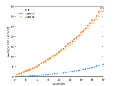
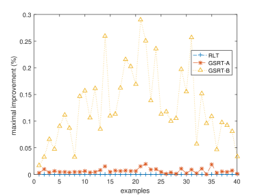
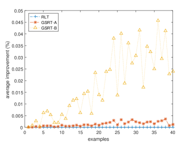
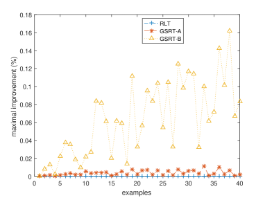
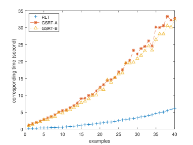
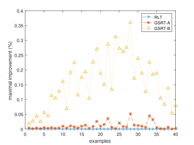
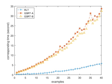
Since we do not know the optimal value of the examples in Table 3, we could not measure the improvement of the GSRT constraint precisely. In the following Figures 1–3, we will show that the improvement can be significant for some class of problems. To measure the effect of the GSRT relaxations, we define the improvement ratio as

$${\rm improv.ratio}=\frac{v({\rm SDP_{GSRT}})-v{\rm(SDP_{RLT})}}{v{\rm(SDP_{RLT})}}.$$

We set the test problems the same as those in Table 3 except that the negative eigenvalues in the quadratic constraints have different number of eigenvalues (which is denoted by $\phi$ in Figures 1–3), and $Q_{0}=I-\sum_{i}^{n}Q_{i}$ to ensure the boundedness of the relaxations. We also set the dimension of the problem as $n=20$, the number of quadratic constraint as $l=5$ and all the quadratic constraints are nonconvex, i.e., $k=0$, and the linear constraints $m$ changing from 1 to 40. For each problem setting, we compute 10 random examples and illustrate the mean and maximal improvement in the figures. From Figures 1–3, we conclude that the improvement is significant with average improvement up to 9%, 5% and 11% and maximal improvement up to 30%, 17% and 36% for cases that $\phi=5$, $\phi=10$ and $\phi=15$, respectively.

Figure 1: Evolution of average and maximal improvement (of 10 examples) versus number of linear constraints for problem setting $n=20$, $\phi=5$.

Figure 2: Evolution of average and maximal improvement versus number of linear constraints for problem setting $n=20$, $\phi=10$.

Figure 3: Evolution of average and maximal improvement versus number of linear constraints for problem setting $n=20$, $\phi=15$.

7 Concluding remark

In this paper, we have presented the GSRT valid inequalities to tighten the SDP relaxations for nonconvex QCQP problems. While the convex relaxations in the current literature lose their effects when dealing with nonconvex quadratic constraints, we decompose each nonconvex quadratic constraint to two convex quadratic constraints and develop GSRT constraints based on the idea of RLT. Specifically, our GSRT constraints extend the SOC-RLT constraint, by linearizing the product of any pair of linear constraint and SOC constraint derived from nonconvex quadratic constraints. Enlightened by the decomposition-approximation method in [31], we have further proposed a tighter relaxation with extra RLT, SOC-RLT and GSRT generated by extra valid linear inequality $\alpha_{u}\geq u^{T}x$. Extending the idea of the GSRT constraints, we have also derived valid inequalities by linearizing the product of any pair of SOC constraints derived from all quadratic constraints. We have finally extended the Kronecker product constraint to GSOC constraints and demonstrated its relationship with the previous relaxations. Promising performance of our numerical tests make us to believe potential applications of our approaches in branch and bound method algorithms for general QCQP problems.

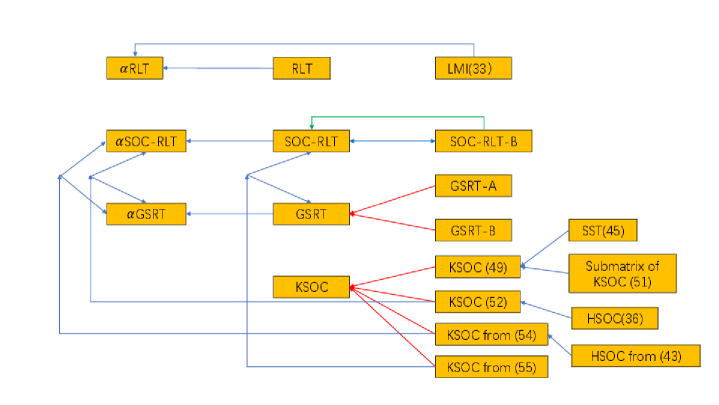
While we extend the reach of the RLT-like techniques for almost all different types of constraint-pairs, we also examine the dominance relationships among them in order to remove these dominated valid inequalities from consideration. We now summarize the dominance relationships of different relaxations discussed in this paper in the following Figure 4.

Figure 4: This figure shows dominance relationships among different valid inequalities. We use $\rm\alpha RLT$, $\rm\alpha SOC\mbox{-}RLT$ and $\rm\alpha GSRT$ to denote different valid inequalities generated from RLT, SOC-RLT and GSRT with a redundant linear inequality $u^{T}x\leq\alpha_{u}$, respectively. A blue arrow indicates the direction of the dominance. i.e., the valid inequality at the tip of the arrow dominates the valid inequality at the bottom of the arrow, e.g., $\rm\alpha RLT$ dominates $\rm RLT$. A red arrow indicates the direction of an inclusion, i.e., the valid inequality at the tip of the arrow includes the valid inequality at the bottom of the arrow, e.g., GSRT includes GSRT-A and GSRT-B. Also note that KSOC (52) and (54) are either dominated by $\rm\alpha GSRT$ or $\rm\alpha SOC\mbox{-}RLT$, depending on whether the SOC (that generates (52) and (54)) is derived from convex or nonconvex quadratic constraints.

In fact, we can further rewrite the objective function as $\min\tau$ and add a new constraint $x_{0}^{T}Q_{0}x_{0}+c_{0}^{T}x\leq\tau$, with a new variable $\tau$. The original problem is then equivalent to minimizing $\tau$ and all the techniques developed in this paper can be applied to the new constraint $x_{0}^{T}Q_{0}x_{0}+c_{0}Tx\leq\tau$ to achieve a tighter lower bound.

An obvious drawback of the relaxations proposed in this paper is their expensive computational cost due to the involved large number of extra SOC constraints, which is a general challenge in RLT based optimization algorithms, see [1, 25]. One direction to overcome this computational difficulty is to avoid solving SDP problems by using, instead, linear inequalities to approximate the linear matrix constraint $X\succeq xx^{T}$, which are also called semidefinite cutting plane method [25] and [22]. Another important observation is that a large number of RLT, SOC-RLT and GSRT constraints are inactive at the optimal solution, which inspires us to consider in our future study the idea of dynamically adding semidefinite cutting planes. More specifically, we can dynamically add some RLT, SOC-RLT and GSRT constraints which are most violated by the current relaxation solution, rather than including all the RLT, SOC-RLT and GSRT constraints in the beginning.

References

- [1] K. Anstreicher. Semidefinite programming versus the reformulation-linearization technique for nonconvex quadratically constrained quadratic programming. J. Global Optim., 43(2-3):471–484, 2009.
- [2] K. Anstreicher. On convex relaxations for quadratically constrained quadratic programming. Math. Program., 136(2):233–251, 2012.
- [3] K. Anstreicher. Kronecker product constraints with an application to the two-trust-region subproblem. SIAM Journal on Optimization, 27(1):368–378, 2017.
- [4] K. Anstreicher, X. Chen, H. Wolkowicz, and Y.-X. Yuan. Strong duality for a trust-region type relaxation of the quadratic assignment problem. Linear Algebra and its Applications, 301(1-3):121–136, 1999.
- [5] K. Anstreicher and H. Wolkowicz. On lagrangian relaxation of quadratic matrix constraints. SIAM Journal on Matrix Analysis and Applications, 22(1):41–55, 2000.
- [6] X. Bao, N. V. Sahinidis, and M. Tawarmalani. Semidefinite relaxations for quadratically constrained quadratic programming: A review and comparisons. Math. Program., 129(1):129–157, 2011.
- [7] A. Beck and Y. C. Eldar. Strong duality in nonconvex quadratic optimization with two quadratic constraints. SIAM J. Optim., 17(3):844–860, 2006.
- [8] A. Ben-Tal and D. den Hertog. Hidden conic quadratic representation of some nonconvex quadratic optimization problems. Math. Program., 143(1-2):1–29, 2014.
- [9] S. Boyd and L. Vandenberghe. Semidefinite programming relaxations of non-convex problems in control and combinatorial optimization. In Communications, Computation, Control, and Signal Processing, pages 279–287. Springer, 1997.
- [10] S. Burer and K. Anstreicher. Second-order-cone constraints for extended trust-region subproblems. SIAM J. Optim., 23(1):432–451, 2013.
- [11] S. Burer and A. Saxena. The MILP road to MIQCP. In Mixed Integer Nonlinear Programming, pages 373–405. Springer, 2012.
- [12] S. Burer and D. Vandenbussche. A finite branch-and-bound algorithm for nonconvex quadratic programming via semidefinite relaxations. Math. Program., 113(2):259–282, 2008.
- [13] S. Burer and B. Yang. The trust region subproblem with non-intersecting linear constraints. Math. Program., 149(1-2):253–264, 2013.
- [14] M. Celis, J. Dennis, and R. Tapia. A trust region strategy for nonlinear equality constrained optimization. Numerical Optimization, 1984:71–82, 1985.
- [15] T. Fujie and M. Kojima. Semidefinite programming relaxation for nonconvex quadratic programs. J. Global Optim, 10(4):367–380, 1997.
- [16] M. Grant and S. Boyd. Graph implementations for nonsmooth convex programs. In V. Blondel, S. Boyd, and H. Kimura, editors, Recent Advances in Learning and Control, Lecture Notes in Control and Information Sciences, pages 95–110. Springer-Verlag Limited, 2008. http://stanford.edu/~boyd/graph_dcp.html.
- [17] M. Grant and S. Boyd. CVX: Matlab software for disciplined convex programming (web page and software), 2009.
- [18] Q. Jin, Y. Tian, Z. Deng, S.-C. Fang, and W. Xing. Exact computable representation of some second-order cone constrained quadratic programming problems. J. Oper. Res. Soc. China, 1(1):107–134, 2013.
- [19] S. Kim, M. Kojima, and K.-C. Toh. A Lagrangian–DNN relaxation: a fast method for computing tight lower bounds for a class of quadratic optimization problems. Math. Program., 156(1-2):161–187, 2016.
- [20] J. Linderoth. A simplicial branch-and-bound algorithm for solving quadratically constrained quadratic programs. Math. Program., 103(2):251–282, 2005.
- [21] P. M. Pardalos and S. A. Vavasis. Quadratic programming with one negative eigenvalue is np-hard. J. Global Optim., 1(1):15–22, 1991.
- [22] A. Qualizza, P. Belotti, and F. Margot. Linear programming relaxations of quadratically constrained quadratic programs. In J. Lee and S. Leyffer, editors, Mixed Integer Nonlinear Programming, pages 407–426. Springer New York, New York, NY, 2012.
- [23] S. Sahni. Computationally related problems. SIAM Journal on Computing, 3(4):262–279, 1974.
- [24] H. D. Sherali and W. P. Adams. A reformulation-linearization technique for solving discrete and continuous nonconvex problems, volume 31. Springer Science & Business Media, 2013.
- [25] H. D. Sherali and B. M. Fraticelli. Enhancing RLT relaxations via a new class of semidefinite cuts. J. Global Optim., 22(1-4):233–261, 2002.
- [26] N. Z. Shor. Quadratic optimization problems. Soviet Journal of Computer and Systems Sciences, 25(6):1–11, 1987.
- [27] J. F. Sturm and S. Zhang. On cones of nonnegative quadratic functions. Math. Oper. Res, 28(2):246–267, 2003.
- [28] Y. Xia, S. Wang, and R.-L. Sheu. S-lemma with equality and its applications. Math. Program., 156(1-2):513–547, 2016.
- [29] B. Yang and S. Burer. A two-variable approach to the two-trust-region subproblem. Manuscript, University of Iowa, February, 2013.
- [30] Y. Ye and S. Zhang. New results on quadratic minimization. SIAM J. Optim., 14(1):245–267, 2003.
- [31] X. J. Zheng, X. L. Sun, and D. Li. Convex relaxations for nonconvex quadratically constrained quadratic programming: matrix cone decomposition and polyhedral approximation. Math. Program., 129(2):301–329, 2011.