Computation of quasilocal effective diffusion tensors and connections to the mathematical theory of homogenization

Abstract

This paper aims at bridging existing theories in numerical and analytical homogenization. For this purpose the multiscale method of Målqvist and Peterseim [Math. Comp. 2014], which is based on orthogonal subspace decomposition, is reinterpreted by means of a discrete integral operator acting on standard finite element spaces. The exponential decay of the involved integral kernel motivates the use of a diagonal approximation and, hence, a localized piecewise constant coefficient. In a periodic setting, the computed localized coefficient is proved to coincide with the classical homogenization limit. An a priori error analysis shows that the local numerical model is appropriate beyond the periodic setting when the localized coefficient satisfies a certain homogenization criterion, which can be verified a posteriori. The results are illustrated in numerical experiments.

Keywords numerical homogenization, multiscale method, upscaling, a priori error estimates, a posteriori error estimates

AMS subject classification 65N12, 65N15, 65N30, 73B27, 74Q05

1 Introduction

Consider the prototypical elliptic model problem

$$-\operatorname{div}A_{\varepsilon}\nabla u=f$$

where the diffusion coefficient $A_{\varepsilon}$ encodes microscopic features on some characteristic length scale $\varepsilon$. Homogenization is a tool of mathematical modeling to identify reduced descriptions of the macroscopic response of such multiscale models in the limit as $\varepsilon$ tends to zero. It turns out that suitable limits represented by the so-called effective or homogenized coefficient exist in fairly general settings in the framework of $G$-, $H$-, or two-scale convergence [Spa68, DG75, MT78, Ngu89, All92]. In general, the effective coefficient is not explicitly given but is rather the result of an implicit representation based on cell problems. This representation usually requires structural assumptions on the sequence of coefficients $A_{\varepsilon}$ such as local periodicity and scale separation [BLP78]. Under such assumptions, efficient numerical methods for the approximate evaluation of the homogenized model are available, e.g., the Heterogeneous Multiscale Method (HMM) [EE03, AEEV12] or the two-scale finite element method [MS02].

In contrast to this idealized setting of analytical homogenization, in practice one is often concerned with one coefficient $A$ with heterogeneities on multiple nonseperable scales and a corresponding sequence of scalable models can hardly be identified or may not be available at all. That is why we are interested in the computation of effective representations of very rough coefficients beyond structural assumptions such as scale separation and local periodicity. In recent years, many numerical attempts have been developed that conceptually do not rely on analytical homogenization results for rough cases. Amongst them are the multiscale finite element method [HW97, EH09], metric-based upscaling [OZ07], hierarchical matrix compression [GH08, Hac15], the flux-norm approach [BO10], generalized finite elements based on spectral cell problems [BL11, EGH13], the AL basis [GGS12, WS15], rough polyharmonic splines [OZB14], iterative numerical homogenization [KY16], and gamblets [Owh17].

Another construction based on concepts of orthogonal subspace decomposition and the solution of localized microscopic cell problems was given in [MP14] and later optimized in [HP13, HMP15, GP15, Pet16]. The method is referred to as the Localized Orthogonal Decomposition (LOD) method. The approach is inspired by ideas of the variational multiscale method [HFMQ98, HS07, Mål11]. As most of the methods above, the LOD constructs a basis representation of some finite-dimensional operator-dependent subspace with superior approximation properties rather than computing an upscaled coefficient. The effective model is then a discrete one represented by the corresponding stiffness matrix and possibly right-hand side. The computation of an effective coefficient is, however, often favorable and this paper re-interprets and modifies the LOD method in this regard.

To this end, we revisit the LOD method of [MP14]. The original method employs finite element basis functions that are modified by a fine-scale correction with a slightly larger support. We show that it is possible to rewrite the method by means of a discrete integral operator acting on standard finite element spaces. The discrete operator is of non-local nature and is not necessarily associated with a differential operator on the energy space $H^{1}_{0}(\Omega)$ (for the physical domain $\Omega\subseteq\mathbb{R}^{d}$). The observation scale $H$ is associated with some quasi-uniform mesh $\mathcal{T}_{H}$ of width $H$. We are able to show that there is a discrete effective non-local model represented by an integral kernel $\mathcal{A}_{H}\in L^{\infty}(\Omega\times\Omega;\mathbb{R}^{d\times d})$ such that the problem is well-posed on a finite-element space $V_{H}$ with similar constants and satisfies

$$\sup_{f\in L^{2}(\Omega)\setminus\{0\}}\frac{\|u(f)-u_{H}(f)\|_{L^{2}(\Omega)}}{\|f\|_{L^{2}(\Omega)}}\lesssim\sup_{f\in L^{2}(\Omega)\setminus\{0\}}\inf_{v_{H}\in V_{H}}\frac{\|u(f)-v_{H}\|_{L^{2}(\Omega)}}{\|f\|_{L^{2}(\Omega)}}+H^{2}.$$

Based on the exponential decay of that kernel $\mathcal{A}_{H}$ away from the diagonal, we propose a quasi-local and sparse formulation as an approximation. The storage requirement for the quasi-local kernel is $\mathcal{O}(H^{-d}\lvert\log H\rvert)$.

For an even stronger compression to $\mathcal{O}(H^{-d})$ information, one can replace $\mathcal{A}_{H}$ by a local and piecewise constant tensor field $A_{H}$. It turns out that this localized effective coefficient $A_{H}$ coincides with the homogenized coefficient of classical homogenization in the periodic case provided that the structure of the coefficient is slightly stronger than only periodic and that the mesh is suitably aligned with the periodicity pattern. In this sense, the results of this paper bridge the multiscale method of [MP14] with classical analytical techniques and numerical methods such as HMM. With regard to the recent reinterpretation of the multiscale method in [KPY16], the paper even connects all the way from analytic homogenization to the theory of iterative solvers.

This new representation of the multiscale method turns out to be particularly attractive for computational stochastic homogenization [GP17]. A further advantage of our numerical techniques when compared with classical analytical techniques is that they are still applicable in the general non-periodic case, where the local numerical model yields reasonable results whenever a certain quantitative homogenization criterion is satisfied, which can be checked a posteriori through a computable model error estimator. Almost optimal convergence rates can be proved under reasonable assumptions on the data.

The structure of this article is as follows. After the preliminaries on the model problem and notation from Section 2, we review the LOD method of [MP14] and introduce the quasi-local effective discrete coefficients in Section 3. In Section 4, we present the error analysis for the localized effective coefficient. Section 5 studies the particular case of a periodic coefficient. We present numerical results in Section 6.

Standard notation on Lebesgue and Sobolev spaces applies throughout this paper. The notation $a\lesssim b$ abbreviates $a\leq Cb$ for some constant $C$ that is independent of the mesh-size, but may depend on the contrast of the coefficient $A$; $a\approx b$ abbreviates $a\lesssim b\lesssim a$. The symmetric part of a quadratic matrix $M$ is denoted by $\operatorname{sym}(M)$.

2 Model problem and notation

This section describes the model problem and some notation on finite element spaces.

2.1 Model problem

Let $\Omega\subseteq\mathbb{R}^{d}$ for $d\in\{1,2,3\}$ be an open Lipschitz polytope. We consider the prototypical model problem

$$-\operatorname{div}(A\nabla u)=f\quad\text{in }\Omega,\qquad u|_{\partial\Omega}=0.$$ (2.1)

The coefficient $A\in L^{\infty}(\Omega;\mathbb{R}^{d\times d})$ is assumed to be symmetric and to satisfy the following uniform spectral bounds

$$0<\alpha\leq\operatorname*{ess\,inf}_{x\in\Omega}\inf_{\xi\in\mathbb{R}^{d}\setminus\{0\}}\frac{\xi\cdot(A(x)\xi)}{\xi\cdot\xi}\leq\operatorname*{ess\,sup}_{x\in\Omega}\sup_{\xi\in\mathbb{R}^{d}\setminus\{0\}}\frac{\xi\cdot(A(x)\xi)}{\xi\cdot\xi}\leq\beta.$$ (2.2)

The symmetry of $A$ is not essential for our analysis and is assumed for simpler notation. The weak form employs the Sobolev space $V:=H^{1}_{0}(\Omega)$ and the bilinear form $a$ defined, for any $v,w\in V$, by

$$a(v,w):=(A\nabla v,\nabla w)_{L^{2}(\Omega)}.$$

Given $f\in L^{2}(\Omega)$ and the linear functional

$$F:V\to\mathbb{R},\quad\text{with }F(v):=\int_{\Omega}fv\,dx\quad\text{ for any }v\in V,$$

the weak form seeks $u\in V$ such that

$$a(u,v)=F(v)\quad\text{for all }v\in V.$$ (2.3)

2.2 Finite element spaces

Let $\mathcal{T}_{H}$ be a quasi-uniform regular triangulation of $\Omega$ and let $V_{H}$ denote the standard $P_{1}$ finite element space, that is, the subspace of $V$ consisting of piecewise first-order polynomials.

Given any subdomain $S\subseteq\overline{\Omega}$, define its neighbourhood via

$$\mathsf{N}(S):=\operatorname{int}\Big{(}\cup\{T\in\mathcal{T}_{H}\,:\,T\cap\overline{S}\neq\emptyset\}\Big{)}.$$

Furthermore, we introduce for any $m\geq 2$ the patch extensions

$$\mathsf{N}^{1}(S):=\mathsf{N}(S)\qquad\text{and}\qquad\mathsf{N}^{m}(S):=\mathsf{N}(\mathsf{N}^{m-1}(S)).$$

Throughout this paper, we assume that the coarse-scale mesh $\mathcal{T}_{H}$ belongs to a family of quasi-uniform triangulations. The global mesh-size reads $H:=\max\{\operatorname{diam}(T):T\in\mathcal{T}_{H}\}$. Note that the shape-regularity implies that there is a uniform bound $C(m)$ on the number of elements in the $m$th-order patch, $\operatorname{card}\{K\in\mathcal{T}_{H}\,:\,K\subseteq\overline{\mathsf{N}^{m}(T)}\}\leq C(m)$ for all ${T\in\mathcal{T}_{H}}$. The constant $C(m)$ depends polynomially on $m$. The set of interior $(d-1)$-dimensional hyper-faces of $\mathcal{T}_{H}$ is denoted by $\mathcal{F}_{H}$. For a piecewise continuous function $\varphi$, we denote the jump across an interior edge by $[\varphi]_{F}$, where the index $F$ will be sometimes omitted for brevity. The space of piecewise constant $d\times d$ matrix fields is denoted by $P_{0}(\mathcal{T}_{H};\mathbb{R}^{d\times d})$.

Let $I_{H}:V\to V_{H}$ be a surjective quasi-interpolation operator that acts as a $H^{1}$-stable and $L^{2}$-stable quasi-local projection in the sense that $I_{H}\circ I_{H}=I_{H}$ and that for any $T\in\mathcal{T}_{H}$ and all $v\in V$ there holds

$$H^{-1}\|v-I_{H}v\|_{L^{2}(T)}+\|\nabla I_{H}v\|_{L^{2}(T)} \leq C_{I_{H}}\|\nabla v\|_{L^{2}(\mathsf{N}(T))}$$ (2.4)

$$\|I_{H}v\|_{L^{2}(T)} \leq C_{I_{H}}\|v\|_{L^{2}(\mathsf{N}(T))}.$$ (2.5)

Since $I_{H}$ is a stable projection from $V$ to $V_{H}$, any $v\in V$ is quasi-optimally approximated by $I_{H}v$ in the $L^{2}(\Omega)$ norm as well as in the $H^{1}(\Omega)$ norm. One possible choice is to define $I_{H}:=E_{H}\circ\Pi_{H}$, where $\Pi_{H}$ is the $L^{2}$ projection onto the space $P_{1}(\mathcal{T}_{H})$ of piecewise affine (possibly discontinuous) functions and $E_{H}$ is the averaging operator that maps $P_{1}(\mathcal{T}_{H})$ to $V_{H}$ by assigning to each free vertex the arithmetic mean of the corresponding function values of the neighbouring cells, that is, for any $v\in P_{1}(\mathcal{T}_{H})$ and any free vertex $z$ of $\mathcal{T}_{H}$,

$$(E_{H}(v))(z)=\sum_{\begin{subarray}{c}T\in\mathcal{T}_{H}\\ \text{with }z\in T\end{subarray}}v|_{T}(z)\bigg{/}\operatorname{card}\{K\in\mathcal{T}_{H}\,:\,z\in K\}.$$ (2.6)

This choice of $I_{H}$ is employed in our numerical experiments.

3 Non-local effective coefficient

We introduce a modified version of the LOD method of [MP14, HP13] and its localization. We give a new interpretation by means of a non-local effective coefficient and present an a priori error estimate.

3.1 A modified LOD method

Let $W:=\operatorname{ker}I_{H}\subseteq V$ denote the kernel of $I_{H}$. Given any $T\in\mathcal{T}_{H}$ and $j\in\{1,\dots,d\}$, the element corrector $q_{T,j}\in W$ is the solution of the variational problem

$$a(w,q_{T,j})=\int_{T}\nabla w\cdot(Ae_{j})\,dx\quad\text{for all }w\in W.$$ (3.1)

Here $e_{j}$ is the $j$-th standard Cartesian unit vector in $\mathbb{R}^{d}$. The gradient of any $v_{H}\in V_{H}$ has the representation

$$\nabla v_{H}=\sum_{T\in\mathcal{T}_{H}}\sum_{j=1}^{d}(\partial_{j}v_{H}|_{T})e_{j}.$$

Given any $v_{H}\in V_{H}$, define the corrector $\mathcal{C}v_{H}$ by

$$\mathcal{C}v_{H}=\sum_{T\in\mathcal{T}_{H}}\sum_{j=1}^{d}(\partial_{j}v_{H}|_{T})q_{T,j}.$$ (3.2)

We remark that for any $v_{H}\in V_{H}$ the gradient $\nabla v_{H}$ is piecewise constant and, thus, $\mathcal{C}v_{H}$ is a finite linear combination of the element correctors $q_{T,j}$. It is readily verified that, for any $v_{H}\in V_{H}$, $\mathcal{C}v_{H}$ is the $a$-orthogonal projection on $W$, i.e.,

$$a(w,v_{H}-\mathcal{C}v_{H})=0\quad\text{for all }w\in W.$$ (3.3)

Clearly, by (3.3), the projection $\mathcal{C}v\in W$ is well-defined for any $v\in V$. The representation (3.2) for discrete functions will, however, be useful in this work.

The LOD method in its version from [MP14] seeks $\bar{u}_{H}\in V_{H}$ such that

$$a((1-\mathcal{C})\bar{u}_{H},(1-\mathcal{C})v_{H})=F((1-\mathcal{C})v_{H})\quad\text{for all }v_{H}\in V_{H}.$$ (3.4)

By (3.3), it is clear that this is equivalent to

$$a(\bar{u}_{H},(1-\mathcal{C})v_{H})=F((1-\mathcal{C})v_{H})\quad\text{for all }v_{H}\in V_{H}.$$ (3.5)

A variant of this multiscale method employs a problem-independent right-hand side and seeks $u_{H}\in V_{H}$ such that

$$a((1-\mathcal{C})u_{H},(1-\mathcal{C})v_{H})=F(v_{H})\quad\text{for all }v_{H}\in V_{H}$$

or, equivalently,

$$a(u_{H},(1-\mathcal{C})v_{H})=F(v_{H})\quad\text{for all }v_{H}\in V_{H}.$$ (3.6)

3.2 Localization of the corrector problems

Here, we briefly describe the localization technique of [MP14]. It was shown in [MP14] and [HP13, Lemma 4.9] that the method is localizable in the sense that any $T\in\mathcal{T}_{H}$ and any $j\in\{1,\dots,d\}$ satisfy

$$\|\nabla q_{T,j}\|_{L^{2}(\Omega\setminus\mathsf{N}^{m}(T))}\lesssim\exp(-cm)\|e_{j}\|_{L^{2}(T)},\qquad m\geq 0.$$ (3.7)

The exponential decay from (3.7) suggests to localize the computation (3.1) of the corrector belonging to an element $T\in\mathcal{T}_{H}$ to a smaller domain, namely the extended element patch $\Omega_{T}:=\mathsf{N}^{\ell}(T)$ of order $\ell$. The nonnegative integer $\ell$ is referred to as the oversampling parameter. Let $W_{\Omega_{T}}\subseteq W$ denote the space of functions from $W$ that vanish outside $\Omega_{T}$. On the patch, in analogy to (3.1), for any $v_{H}\in V_{H}$, any $T\in\mathcal{T}_{H}$ and any $j\in\{1,\dots,d\}$, the function $q_{T,j}^{(\ell)}\in W_{\Omega_{T}}$ solves

$$\int_{\Omega_{T}}\nabla w\cdot(A\nabla q_{T,j}^{(\ell)})\,dx=\int_{T}\nabla w\cdot(Ae_{j})\,dx\quad\text{for all }w\in W_{\Omega_{T}}.$$ (3.8)

Given $v_{H}\in V_{H}$, we define the corrector $\mathcal{C}^{(\ell)}v_{H}\in W$ by

$$\mathcal{C}^{(\ell)}v_{H}=\sum_{T\in\mathcal{T}_{H}}\sum_{j=1}^{d}(\partial_{j}v_{H}|_{T})q_{T,j}^{(\ell)}.$$ (3.9)

A practical variant of (3.6) is to seek $u_{H}^{(\ell)}\in V_{H}$ such that

$$a(u_{H}^{(\ell)},(1-\mathcal{C}^{(\ell)})v_{H})=F(v_{H})\quad\text{for all }v_{H}\in V_{H}.$$ (3.10)

This procedure is indispensable for actual computations and the effect of the truncation of the domain on the error of the multiscale method was analyzed in [MP14] and [HP13]. We will provide the error analysis for the method (3.10) in Subsection 3.4 below.

3.3 Definition of the quasi-local effective coefficient

In this subsection, we do not make any specific choice for the oversampling parameter $\ell$. In particular, the analysis covers the case that all element patches $\Omega_{T}$ equal the whole domain $\Omega$. We denote the latter case formally by $\ell=\infty$.

We re-interpret the left-hand side of (3.10) as a non-local operator acting on standard finite element functions. To this end, consider any $u_{H},v_{H}\in V_{H}$. We have

$$a(u_{H},(1-\mathcal{C}^{(\ell)})v_{H})=\int_{\Omega}\nabla u_{H}\cdot(A\nabla v_{H})\,dx-\int_{\Omega}\nabla u_{H}\cdot(A\mathcal{C}^{(\ell)}\nabla v_{H})\,dx.$$

The second term can be expanded with (3.9) as

$$\int_{\Omega}\nabla u_{H}\cdot(A\nabla\mathcal{C}^{(\ell)}v_{H})\,dx$$

$$\qquad=\sum_{T\in\mathcal{T}_{H}}\sum_{k=1}^{d}(\partial_{k}v_{H}|_{T})\int_{\Omega}\nabla u_{H}\cdot(A\nabla q_{T,k}^{(\ell)})\,dx$$

$$\qquad=\sum_{K,T\in\mathcal{T}_{H}}\int_{K}\nabla u_{H}\cdot\left(\sum_{k=1}^{d}\fint_{K}(A(y)\nabla q_{T,k}^{(\ell)}(y))\,dy\;(\partial_{k}v_{H}|_{T})\right)\,dx$$

$$\qquad=\sum_{K,T\in\mathcal{T}_{H}}\lvert K\rvert\,\lvert T\rvert\;\nabla u_{H}|_{K}\cdot(\mathcal{K}_{T,K}\nabla v_{H}|_{T})$$

for the matrix $\mathcal{K}_{T,K}^{(\ell)}$ defined for any $K,T\in\mathcal{T}_{H}$ by

$$(\mathcal{K}_{T,K}^{(\ell)})_{j,k}:=\frac{1}{|T|\,|K|}e_{j}\cdot\int_{K}A\nabla q_{T,k}^{(\ell)}\,dx.$$

Define the piecewise constant matrix field over $\mathcal{T}_{H}\times\mathcal{T}_{H}$, for $T,K\in\mathcal{T}_{H}$ by

$$\mathcal{A}_{H}^{(\ell)}|_{T,K}:=\frac{\delta_{T,K}}{|K|}\fint_{T}A\,dx-\mathcal{K}_{T,K}^{(\ell)}$$

(where $\delta$ is the Kronecker symbol) and the bilinear form $\mathfrak{a}^{(\ell)}$ on $V_{H}\times V_{H}$ by

$$\mathfrak{a}^{(\ell)}(v_{H},z_{H}):=\int_{\Omega}\int_{\Omega}\nabla v_{H}(y)\cdot(\mathcal{A}_{H}^{(\ell)}(x,y)\nabla z_{H}(x))\,dy\,dx\quad\text{for any }v_{H},z_{H}\in V_{H}.$$

We obtain for all $v_{H},z_{H}\in V_{H}$ that

$$a(v_{H},(1-\mathcal{C}^{(\ell)})z_{H})=\mathfrak{a}^{(\ell)}(v_{H},z_{H}).$$ (3.11)

Remark 1 (notation).

For simplices $T,K\in\mathcal{T}_{H}$ with $x\in T$ and $y\in K$, we will sometimes write $\mathcal{K}^{(\ell)}(x,y)$ instead of $\mathcal{K}_{T,K}^{(\ell)}$ (with analogous notation for $\mathcal{A}^{(\ell)}$).

Next, we state the equivalence of two multiscale formulations.

Proposition 2.

A function $u_{H}^{(\ell)}\in V_{H}$ solves (3.10) if and only if it solves

$$\mathfrak{a}^{(\ell)}(u_{H}^{(\ell)},v_{H})=F(v_{H}).$$ (3.12)

Proof.

This follows directly from the representation (3.11). ∎

Remark 3.

For $d=1$ and $I_{H}$ the standard nodal interpolation operator, the corrector problems localize to one element and the presented multiscale approach coincides with various known methods (homogenization, MSFEM). The resulting effective coefficient $\mathcal{A}_{H}^{(\ell)}$ is diagonal and, thus, local. This is no longer the case for $d\geq 2$.

3.4 Error analysis

This subsection presents an error estimate for the error produced by the method (3.10) (and so by the method (3.12)). We begin by briefly summarizing some results from [MP14].

Lemma 4.

Let $u\in V$ solve (2.3) and $\bar{u}_{H}\in V_{H}$ solve (3.4). Then we have the following properties.

• $\bar{u}_{H}$ coincides with the quasi-interpolation of $u$, i.e., $\bar{u}_{H}=I_{H}u$.

• The Galerkin orthogonality $a(u-(1-\mathcal{C})I_{H}u,(1-\mathcal{C})v_{H})=0$ for all $v_{H}\in V_{H}$ is satisfied.

• The error satisfies $\|\nabla(u-(1-\mathcal{C})\bar{u}_{H})\|_{L^{2}(\Omega)}\lesssim H\|f\|_{L^{2}(\Omega)}$.

Proof.

See [MP14] for proofs. ∎

We define the following worst-case best-approximation error

$$\bm{\mathrm{wcba}}(A,\mathcal{T}_{H}):=\sup_{g\in L^{2}(\Omega)\setminus\{0\}}\inf_{v_{H}\in V_{H}}\frac{\|u(g)-v_{H}\|_{L^{2}(\Omega)}}{\|g\|_{L^{2}(\Omega)}}$$ (3.13)

where for $g\in L^{2}(\Omega)$, $u(g)\in V$ solves (2.3) with right-hand side $g$. Standard interpolation and stability estimates show that always $\bm{\mathrm{wcba}}(A,\mathcal{T}_{H})\lesssim H$, but it may behave better in certain regimes. E.g., in a periodic homogenization problem with some small parameter $\varepsilon$ and some smooth homogenized solution $u_{0}\in H^{2}(\Omega)$, the best approximation error is dominated by the best approximation error of $u_{0}$ in the regime $H\lesssim\sqrt{\varepsilon}$ where it scales like $H^{2}$. By contrast, the error is typically not improved in the regime $\sqrt{\varepsilon}\gtrsim H\gtrsim\varepsilon$. This non-linear behavior of the best-approximation error in the pre-asymptotic regime is prototypical for homogenization problems with scale separation and explains why the rough bound $H$ is suboptimal.

The following result states an $L^{2}$ error estimate for the method (3.6). The result is surprising because the perturbation of the right-hand side seems to be of order $H$ at first glance. In cases of scale separation the quadratic rate is indeed observed in the regime $H\lesssim\sqrt{\varepsilon}$ and cannot be explained by naive estimates.

Proposition 5.

The solutions $u\in V$ to (2.3) and $u_{H}\in V_{H}$ to (3.6) for right-hand side $f\in L^{2}(\Omega)$ satisfy the following error estimate

$$\frac{\|u-u_{H}\|_{L^{2}(\Omega)}}{\|f\|_{L^{2}(\Omega)}}\lesssim H^{2}+\bm{\mathrm{wcba}}(A,\mathcal{T}_{H}).$$

Proof.

Let $f\in L^{2}(\Omega)\setminus\{0\}$ and let $\bar{u}_{H}\in V_{H}$ solve (3.5). We begin by analyzing the error $e_{H}:=u_{H}-\bar{u}_{H}$. Let $z\in V$ denote the solution to

$$a(v,z)=(e_{H},I_{H}v)_{L^{2}(\Omega)}\quad\text{for all }v\in V.$$

To see that the right-hand side is indeed represented by an $L^{2}$ function, note that $I_{H}$ is continuous on $L^{2}(\Omega)$ and, hence, the right-hand side has a Riesz representative $\tilde{e}\in L^{2}(\Omega)$ such that $(e_{H},I_{H}v)_{L^{2}(\Omega)}=(\tilde{e},v)_{L^{2}(\Omega)}$. In particular, $z$ solves (2.3) with right-hand side $\tilde{e}$. Its $L^{2}$ norm is bounded with (2.5) as follows

$$\|\tilde{e}\|_{L^{2}(\Omega)}^{2}=(e_{H},I_{H}\tilde{e}_{H})_{L^{2}(\Omega)}\lesssim\|e_{H}\|_{L^{2}(\Omega)}\|\tilde{e}\|_{L^{2}(\Omega)},$$

hence

$$\|\tilde{e}\|_{L^{2}(\Omega)}\lesssim\|e_{H}\|_{L^{2}(\Omega)}.$$ (3.14)

We note that, for any $w\in W$, we have $a(w,z)=(e_{H},I_{H}w)_{L^{2}(\Omega)}=0$. Thus, we have $a(e_{H},\mathcal{C}z)=a(\mathcal{C}e_{H},z)=0$. With $(1-\mathcal{C})z=(1-\mathcal{C})I_{H}z$ we conclude

$$\|e_{H}\|_{L^{2}(\Omega)}^{2}=a(e_{H},z)=a(e_{H},(1-\mathcal{C})I_{H}z).$$ (3.15)

Elementary algebraic manipulations with the projection $I_{H}$ show that

$$-\mathcal{C}I_{H}z=(1-I_{H})\big{(}(1-\mathcal{C})I_{H}z-z\big{)}+(1-I_{H})z.$$

The relation (3.15) and the solution properties (3.5) and (3.6), thus, lead to

$$\|e_{H}\|_{L^{2}(\Omega)}^{2}=F(\mathcal{C}I_{H}z)=\lvert F((1-I_{H})((1-\mathcal{C})I_{H}z-z))+F((1-I_{H})z)\rvert.$$ (3.16)

We proceed by estimating the two terms on the right-hand side of (3.16) separately. For the second term in (3.16), the $L^{2}$-best approximation property of $I_{H}$ and (3.14) reveal

$$\lvert F((1-I_{H})z)\rvert \lesssim\|f\|_{L^{2}(\Omega)}\|\tilde{e}\|_{L^{2}(\Omega)}\inf_{v_{H}\in V_{H}}\frac{\|z-v_{H}\|_{L^{2}(\Omega)}}{\|\tilde{e}\|_{L^{2}(\Omega)}}$$ (3.17)

$$\lesssim\|f\|_{L^{2}(\Omega)}\|e_{H}\|_{L^{2}(\Omega)}\bm{\mathrm{wcba}}(A,\mathcal{T}_{H}).$$

For the first term in (3.16), we obtain with the stability of $I_{H}$ and the Cauchy inequality that

$$\lvert F((1-I_{H})((1-\mathcal{C})I_{H}z-z))\rvert\lesssim\|f\|_{L^{2}(\Omega)}\|z-(1-\mathcal{C})I_{H}z\|_{L^{2}(\Omega)}.$$

Let $\tilde{g}:=z-(1-\mathcal{C})I_{H}z$ and let $\zeta\in V$ denote the solution to

$$a(\zeta,v)=(\tilde{g},v)_{L^{2}(\Omega)}\quad\text{for all }v\in V.$$

As stated in Lemma 4(i), the function $I_{H}z\in V_{H}$ is the Galerkin approximation to $z$ with method (3.4) with right-hand side $\tilde{e}$. We, thus, have by symmetry of $a$ and the Galerkin orthogonality from Lemma 4(ii) that

$$\|z-(1-\mathcal{C})I_{H}z\|_{L^{2}(\Omega)}^{2} =a(\zeta,z-(1-\mathcal{C})I_{H}z)$$

$$=a(\zeta-(1-\mathcal{C})I_{H}\zeta,z-(1-\mathcal{C})I_{H}z).$$

Continuity of $a$ and Lemma 4(iii) reveal that this is bounded by

$$H^{2}\|\tilde{g}\|_{L^{2}(\Omega)}\|\tilde{e}\|_{L^{2}(\Omega)}=H^{2}\|z-(1-\mathcal{C})I_{H}z\|_{L^{2}(\Omega)}\|\tilde{e}\|_{L^{2}(\Omega)}.$$

Altogether, with (3.16),

$$\frac{\|e_{H}\|_{L^{2}(\Omega)}}{\|f\|_{L^{2}(\Omega)}}\lesssim H^{2}+\bm{\mathrm{wcba}}(A,\mathcal{T}_{H}).$$

Since

$$\frac{\|u-\bar{u}_{H}\|_{L^{2}(\Omega)}}{\|f\|_{L^{2}(\Omega)}}\lesssim\bm{\mathrm{wcba}}(A,\mathcal{T}_{H}),$$

(which follows from the fact that $\bar{u}_{H}=I_{H}u$), the triangle inequality concludes the proof. ∎

With similar arguments it is possible to prove that the coupling $\ell\approx\lvert\log H\rvert$ is sufficient to derive the error bound

$$\|u-u_{H}^{(\ell)}\|_{L^{2}(\Omega)}\lesssim(H^{2}+\bm{\mathrm{wcba}}(A,\mathcal{T}_{H}))\,\|f\|_{L^{2}(\Omega)}.$$ (3.18)

The proof is based on a similar argument as in Proposition 5: Since the $L^{2}$ distance of $u-\bar{u}_{H}^{(\ell)}$ is controlled by the right-hand side of (3.18) [HP13] where $\bar{u}_{H}^{(\ell)}$ solves a modified version of (3.10) with right-hand side $F((1-\mathcal{C}^{(\ell)})v_{H})$, it is sufficient to control $u_{H}^{(\ell)}-\bar{u}_{H}^{(\ell)}$ in the $L^{2}$ norm. This can be done with a duality argument similar to that from the proof of Proposition 5. The additional tool needed therein is the fact that

$$\|\nabla(\mathcal{C}-\mathcal{C}^{(\ell)})I_{H}z\|_{L^{2}(\Omega)}\lesssim\exp(-c\ell)C(\ell)\|\nabla z\|_{L^{2}(\Omega)}$$

for the dual solution $z$ (see [HP13, Proof of Thm. 4.13] for an outline of a proof) where $C(\ell)$ is an overlap constant depending polynomially on $\ell$. The choice of $\ell\approx\lvert\log H\rvert$ therefore leads to (3.18). The details are omitted here and the reader is referred to [MP14, HP13, Pet16, KPY16].

4 Local effective coefficient

Throughout this section we consider oversampling parameters chosen as $\ell\approx\lvert\log H\rvert$.

4.1 Definition of the local effective coefficient

The exponential decay motivates to approximate the non-local bilinear form $\mathfrak{a}^{(\ell)}(\cdot,\cdot)$ by a quadrature-like procedure: Define the piecewise constant coefficient $A_{H}^{(\ell)}\in P_{0}(\mathcal{T}_{H};\mathbb{R}^{d\times d})$ by

$$A_{H}^{(\ell)}|_{T}:=\fint_{T}A\,dx-\sum_{K\in\mathcal{T}_{H}}|K|\,\mathcal{K}_{T,K}^{(\ell)}.$$

and the bilinear form $\tilde{a}^{(\ell)}$ on $V\times V$ by

$$\tilde{a}^{(\ell)}(u,v):=\int_{\Omega}\nabla u\cdot(A_{H}^{(\ell)}\nabla v)\,dx.$$

Remark 6.

In analogy to classical periodic homogenization, the local effective coefficient $A_{H}^{(\ell)}$ can be written as

$$(A_{H}^{(\ell)})_{j,k}|_{T} =|T|^{-1}\int_{\Omega_{T}}e_{j}\cdot\big{(}A(\chi_{T}e_{k}-\nabla q_{T,k}^{(\ell)})\big{)}$$

$$=|T|^{-1}\int_{\Omega_{T}}(e_{j}-\nabla q_{T,j}^{(\ell)})\cdot\big{(}A(\chi_{T}e_{k}-\nabla q_{T,k}^{(\ell)})\big{)}$$

for the characteristic function $\chi_{T}$ of $T$ and the slightly enlarged averaging domain $\Omega_{T}$. See Section 5 for further analogies to homogenization theory in the periodic case.

The localized multiscale method is to seek $\tilde{u}_{H}^{(\ell)}\in V_{H}$ such that

$$\tilde{a}^{(\ell)}(\tilde{u}_{H}^{(\ell)},v_{H})=F(v_{H})\quad\text{for all }v_{H}\in V_{H}.$$ (4.1)

The unique solvability of (4.1) is not guaranteed a priori. It must be checked a posteriori whether positive spectral bounds $\alpha_{H}$, $\beta_{H}$ on $A_{H}^{(\ell)}$ exist in the sense of (2.2). Throughout this paper we assume that such bounds exist, that is, we assume that there exist positive numbers $\alpha_{H}$, $\beta_{H}$ such that

$$\alpha_{H}|\xi|^{2}\leq\xi\cdot(A_{H}^{(\ell)}(x)\xi)\leq\beta_{H}|\xi|^{2}$$ (4.2)

for all $\xi\in\mathbb{R}^{d}$ and almost all $x\in\Omega$.

4.2 Error analysis

The goal of this section is to establish an error estimate for the error

$$\|u-\tilde{u}_{H}^{(\ell)}\|_{L^{2}(\Omega)}.$$

Let $u_{H}^{(\ell)}\in V_{H}$ solve (3.10). Then the error estimate (3.18) leads to the a priori error estimate

$$\|u-u_{H}^{(\ell)}\|_{L^{2}(\Omega)}\lesssim(H^{2}+\bm{\mathrm{wcba}}(A,\mathcal{T}_{H}))\,\|f\|_{L^{2}(\Omega)}.$$ (4.3)

We employ the triangle inequality and merely estimate the difference $\|u_{H}^{(\ell)}-\tilde{u}_{H}^{(\ell)}\|_{L^{2}(\Omega)}$.

With the finite localization parameter $\ell$, the quasi-local coefficient $\mathcal{A}^{(\ell)}$ is sparse in the sense that $\mathcal{A}^{(\ell)}(x,y)=0$ whenever $|x-y|>C\ell H$. We note the following lemma which will be employed in the error analysis.

Lemma 7.

Given some $x\in\Omega$ with $x\in T$ for some $T\in\mathcal{T}_{H}$, we have

$$\|\mathcal{K}^{(\ell)}(x,y)\|_{L^{2}(\Omega,dy)}\lesssim H^{-d/2}.$$

Proof.

From the definition of $\mathcal{K}^{(\ell)}$, the boundedness of $A$ and the Hölder inequality we obtain for any $j,k\in\{1,\dots,d\}$ that

$$|(\mathcal{K}^{(\ell)}_{T,K})_{j,k}|\lesssim\frac{1}{|T|\,|K|}\|\nabla q_{T,k}\|_{L^{1}(K)}\lesssim\frac{1}{|T|\,|K|^{1/2}}\|\nabla q_{T,k}\|_{L^{2}(K)}.$$

Hence, we conclude with the stability of problem (3.8) and $\|e_{k}\|_{L^{2}(T)}^{2}=|T|$ that

$$\|\mathcal{K}^{(\ell)}(x,y)\|_{L^{2}(\Omega,dy)}^{2}=\sum_{K\in\mathcal{T}_{H}}|K||\mathcal{K}^{(\ell)}_{T,K}|^{2}=|T|^{-2}\|\nabla q_{T,k}\|_{L^{2}(\Omega)}^{2}\lesssim H^{-d}.$$

This implies the assertion. ∎

In what follows, we abbreviate

$$\rho:=CH\lvert\log H\rvert$$ (4.4)

for some appropriately chosen constant $C$.

Proposition 8 (error estimate I).

Assume that (4.2) is satisfied. Let $u_{H}^{(\ell)}\in V_{H}$ solve (3.12) and let $\tilde{u}_{H}^{(\ell)}$ solve (4.1). Then,

$$\|\nabla(u_{H}^{(\ell)}-\tilde{u}_{H}^{(\ell)})\|_{L^{2}(\Omega)}\lesssim H^{-d/2}\Big{\|}\|\nabla\tilde{u}_{H}^{(\ell)}(y)-\nabla\tilde{u}_{H}^{(\ell)}(x)\|_{L^{2}(B_{\rho}(x),dy)}\Big{\|}_{L^{2}(\Omega,dx)}.$$

Proof.

Denote $e_{H}:=\tilde{u}_{H}^{(\ell)}-u_{H}^{(\ell)}$. In the idealized case, $\ell=\infty$, the orthogonality (3.3) and relation (3.11) show that

$$\|\nabla(1-\mathcal{C}^{(\ell)})e_{H}\|_{L^{2}(\Omega)}^{2}\lesssim\mathfrak{a}^{(\ell)}(e_{H},e_{H}).$$

The case $\ell\gtrsim|\log H|$ again follows ideas from [MP14] with the exponential-in-$\ell$ closeness of $\mathcal{C}$ and $\mathcal{C}_{\ell}$ and is merely sketched here. From the stability of $I_{H}$ and the properties of the fine-scale projection $\mathcal{C}^{(\ell)}$ we observe (with contrast-dependent constants)

$$\|\nabla e_{H}\|_{L^{2}(\Omega)}^{2}=\|\nabla I_{H}e_{H}\|_{L^{2}(\Omega)}^{2} =\|\nabla I_{H}(1-\mathcal{C}^{(\ell)})e_{H}\|_{L^{2}(\Omega)}^{2}$$

$$\lesssim\|\nabla(1-\mathcal{C}^{(\ell)})e_{H}\|_{L^{2}(\Omega)}^{2}$$

$$\lesssim\mathfrak{a}^{(\ell)}(e_{H},e_{H})+\exp(-c\ell)\|\nabla e_{H}\|_{L^{2}(\Omega)}^{2}$$

for some constant $c>0$. Hence, with positive constants $C_{1}$, $C_{2}$,

$$\|\nabla e_{H}\|_{L^{2}(\Omega)}^{2}\leq C_{1}\mathfrak{a}^{(\ell)}(e_{H},e_{H})+C_{2}\exp(-c\ell)\|\nabla e_{H}\|_{L^{2}(\Omega)}^{2}.$$

If, for some sufficiently large $r$, the parameter $\ell$ is chosen to satisfy $\ell\geq r\lvert\log H\rvert$ such that $C_{2}\exp(-c\ell)\leq 1/2$, then the second term on the right-hand side can be absorbed. Thus, we proceed with (3.12) and (4.1) as

$$\|\nabla e_{H}\|_{L^{2}(\Omega)}^{2}\lesssim\mathfrak{a}^{(\ell)}(\tilde{u}_{H}^{(\ell)}-u_{H}^{(\ell)},e_{H})=\mathfrak{a}^{(\ell)}(\tilde{u}_{H}^{(\ell)},e_{H})-\tilde{a}^{(\ell)}(\tilde{u}_{H}^{(\ell)},e_{H}).$$

The right-hand side can be rewritten as

$$\mathfrak{a}^{(\ell)}(\tilde{u}_{H}^{(\ell)},e_{H})-\tilde{a}^{(\ell)}(\tilde{u}_{H}^{(\ell)},e_{H})$$

$$=\int_{\Omega}\int_{\Omega}(\nabla\tilde{u}_{H}^{(\ell)}(y)-\nabla\tilde{u}_{H}^{(\ell)}(x))\cdot\bigg{[}\mathcal{A}_{H}^{(\ell)}(x,y)\nabla e_{H}(x)\bigg{]}\,dy\,dx$$

$$\quad+\int_{\Omega}\bigg{[}\tilde{u}_{H}^{(\ell)}(x)\cdot\left(\int_{\Omega}\mathcal{A}_{H}^{(\ell)}(x,y)\,dy-A_{H}^{(\ell)}(x)\right)\nabla e_{H}(x)\bigg{]}\,dx.$$

The second term vanishes by definition of $A_{H}^{(\ell)}$. Hence, the combination of the preceding arguments with the Cauchy inequality leads to

$$\|\nabla e_{H}\|_{L^{2}(\Omega)}^{2}\lesssim\|\nabla e_{H}\|_{L^{2}(\Omega)}\Big{\|}\int_{B_{\rho}(x)}\mathcal{A}_{H}^{(\ell)}(x,y)^{*}(\nabla\tilde{u}_{H}^{(\ell)}(y)-\nabla\tilde{u}_{H}^{(\ell)}(x))\,dy\Big{\|}_{L^{2}(\Omega,dx)},$$

where it was used that $\mathcal{A}_{H}^{(\ell)}(x,y)=0$ whenever $|x-y|>\rho$. Note that $(\nabla\tilde{u}_{H}^{(\ell)}(y)-\nabla\tilde{u}_{H}^{(\ell)}(x))=0$ for all $x$ and $y$ that belong to the same element $T\in\mathcal{T}_{H}$. Thus, $\mathcal{A}_{H}^{(\ell)}(x,y)$ in the above expression can be replaced by $\mathcal{K}_{H}^{(\ell)}(x,y)$. This and division by $\|\nabla e_{H}\|_{L^{2}(\Omega)}$ lead to

$$\|\nabla e_{H}\|_{L^{2}(\Omega)}$$ (4.5)

$$\qquad\lesssim\sqrt{\phantom{.}}\left(\int_{\Omega}\bigg{|}\int_{B_{\rho}(x)}\mathcal{K}^{(\ell)}(x,y)^{*}(\nabla\tilde{u}_{H}^{(\ell)}(y)-\nabla\tilde{u}_{H}^{(\ell)}(x))\,dy\bigg{|}^{2}dx\right).$$

This term can be bounded with the Cauchy inequality and Lemma 7 by

$$\quad\sqrt{\phantom{.}}\left(\int_{\Omega}\bigg{|}\|\mathcal{K}^{(\ell)}(x,y)\|_{L^{2}(B_{\rho}(x),dy)}\|\nabla\tilde{u}_{H}^{(\ell)}(y)-\nabla\tilde{u}_{H}^{(\ell)}(x)\|_{L^{2}(B_{\rho}(x),dy)}\bigg{|}^{2}\,dx\right)$$

$$\qquad\lesssim H^{-d/2}\Big{\|}\|\nabla\tilde{u}_{H}^{(\ell)}(y)-\nabla\tilde{u}_{H}^{(\ell)}(x)\|_{L^{2}(B_{\rho}(x),dy)}\Big{\|}_{L^{2}(\Omega,dx)}.$$

This finishes the proof. ∎

It is worth noting that the error bound in Proposition 8 can be evaluated without knowledge of the exact solution. Hence, Proposition 8 can be regarded as an a posteriori error estimate. Formula (4.5) could also be an option if it is available. We expect Proposition 8 to be rather sharp. Below we provide the main a priori error estimate, Proposition 10, which is fundamental for the mentioned link between analytical and numerical homogenization. The following technical lemma is required.

Lemma 9 (existence of a regularized coefficient).

Let $A_{H}\in P_{0}(\mathcal{T}_{H};\mathbb{R}^{d\times d})$ be a piecewise constant field of $d\times d$ matrices that satisfies the spectral bounds (4.2). Then there exists a Lipschitz continuous coefficient $A_{H}^{\mathit{reg}}\in W^{1,\infty}(\Omega;\mathbb{R}^{d\times d})$ satisfying the following three properties. 1) The piecewise integral mean is conserved, i.e.,

$$\int_{T}A_{H}^{\mathit{reg}}\,dx=\int_{T}A_{H}\,dx\quad\text{for all }T\in\mathcal{T}_{H}.$$

2) The eigenvalues of $\operatorname{sym}(A_{H}^{\mathit{reg}})$ lie in the interval $[\alpha_{H}/2,2\beta_{H}]$. 3) The derivative satisfies the bound

$$\|\nabla A_{H}^{\mathit{reg}}\|_{L^{\infty}(\Omega)}\leq C\eta(A_{H})$$

for some constant $C$ that depends on the shape-regularity of $\mathcal{T}_{H}$ and for the expression

$$\eta(A_{H}):=H^{-1}\|[A_{H}]\|_{L^{\infty}(\mathcal{F}_{H})}\big{(}1+\alpha_{H}^{-1}\|[A_{H}]\|_{L^{\infty}(\mathcal{F}_{H})}\big{)}.$$ (4.6)

Here $[\cdot]$ defines the inter-element jump and $\mathcal{F}_{H}$ denotes the set of interior hyper-faces of $\mathcal{T}_{H}$.

Proof.

Consider a refined triangulation $\mathcal{T}_{L}$ resulting from $L$ uniform refinements of $\mathcal{T}_{H}$. In particular, the mesh-size in $\mathcal{T}_{L}$ is of the order $2^{-L}H$. Let $E_{L}A_{H}$ denote the $\mathcal{T}_{L}$-piecewise affine and continuous function that takes at every interior vertex the arithmetic mean of the nodal values of $A_{H}$ on the adjacent elements of $\mathcal{T}_{L}$ (similar to (2.6)). Clearly, for this convex combination the eigenvalues of $\operatorname{sym}(E_{L}A_{H})$ range within the interval $[\alpha_{H},\beta_{H}]$. It is not difficult to prove that, for any $T\in\mathcal{T}_{H}$,

$$\fint_{T}|A_{H}-E_{L}A_{H}|\,dx\lesssim 2^{-L}\|[A_{H}]\|_{L^{\infty}(\mathcal{F}_{H}(\omega_{T}))}$$ (4.7)

as well as

$$\|A_{H}-E_{L}A_{H}\|_{L^{\infty}(T)}\lesssim\|[A_{H}]\|_{L^{\infty}(\mathcal{F}_{H}(\omega_{T}))}.$$ (4.8)

Here, $\mathcal{F}_{H}(\omega_{T})$ denotes the set of interior hyper-faces of $\mathcal{T}_{H}$ that share a point with $T$. Let, for any $T\in\mathcal{T}_{H}$, $b_{T}\in H^{1}_{0}(T)$ denote a positive polynomial bubble function with $\fint_{T}b_{T}\,dx=1$ and $\|b_{T}\|_{L^{\infty}(T)}\approx 1$. The regularized coefficient $A_{H}^{\mathit{reg}}=E_{L}(A_{H})+b_{T}\fint_{T}(A_{H}-E_{L}(A_{H}))\,dx$ has, for any $T\in\mathcal{T}_{H}$, the integral mean $\fint_{T}A_{H}^{\mathit{reg}}\,dx=\fint_{T}A_{H}\,dx$. For any $\xi\in\mathbb{R}^{d}$ with $|\xi|=1$ and any $T\in\mathcal{T}_{H}$, the estimate (4.7) shows

$$\left|\xi\cdot\fint_{T}(A_{H}-E_{L}A_{H})\,dx\;b_{T}\xi\right| \leq\left|\fint_{T}(A_{H}-E_{L}A_{H})\,dx\;b_{T}\right|$$

$$\leq C2^{-L}\|[A_{H}]\|_{L^{\infty}(\mathcal{F}_{H}(\omega_{T}))}.$$

If $L$ is chosen to be of the order $\lvert\log(\alpha_{H}^{-1}C\|[A_{H}]\|_{L^{\infty}(\mathcal{F}_{H})})\rvert$ (for small jumps of $A_{H}$ it can be chosen of order $1$), then

$$\left|\xi\cdot\fint_{T}(A_{H}-E_{L}A_{H})\,dx\;b_{T}\xi\right|\leq\alpha/2.$$

This and the triangle inequality prove the claimed spectral bound on $\operatorname{sym}(A_{H}^{\mathit{reg}})$. For the bound on the derivative of $A_{H}^{\mathit{reg}}$, let $t\in T_{L}$ and $T\in\mathcal{T}_{H}$ such that $t\subseteq T$. The diameter of $t$ is of order $2^{-L}H$. Since $\|\nabla b_{T}\|_{L^{\infty}(T)}\lesssim H^{-1}$, the triangle and inverse inequalities therefore yield with the above choice of $L$ (note that $\nabla(A_{H}|_{T})=0$)

$$\|\nabla A_{H}^{\mathit{reg}}\|_{L^{\infty}(t)} \lesssim\|\nabla(A_{H}-E_{L}(A_{H}))\|_{L^{\infty}(t)}+H^{-1}\|A_{H}-E_{L}(A_{H})\|_{L^{\infty}(t)}$$

$$\lesssim H^{-1}\|[A_{H}]\|_{L^{\infty}(\mathcal{F}_{H}(\omega_{T}))}\big{(}1+\alpha_{H}^{-1}\|[A_{H}]\|_{L^{\infty}(\mathcal{F}_{H}(\omega_{T})}\big{)}.$$

This proves the assertion. ∎

By Lemma 9, there exists a coefficient $A_{H}^{\mathit{reg}}\in W^{1,\infty}(\Omega)$ such that $A_{H}^{(\ell)}$ is the piecewise $L^{2}$ projection of $A_{H}^{\mathit{reg}}$ onto the piecewise constants. Let $u^{\mathit{reg}}\in V$ solve

$$\int_{\Omega}\nabla{u^{\mathit{reg}}}\cdot(A_{H}^{\mathit{reg}}\nabla v)\,dx=F(v)\quad\text{for all }v\in V.$$ (4.9)

In particular, $\tilde{u}_{H}$ is the finite element approximation to $u^{\mathit{reg}}$. In the following, $s$ refers to the $H^{1+s}(\Omega)$ regularity index of a function. Recall that the $H^{1+s}(\Omega)$ norm [Ada75] of some a function $v$ is given by

$$\|v\|_{H^{1+s}(\Omega)}=\left[\|v\|_{H^{1}(\Omega)}^{2}+\int_{\Omega}\int_{\Omega}\frac{|\nabla v(x)-\nabla v(y)|^{2}}{\lvert x-y\rvert^{d+2s}}\,dy\,dx\right]^{1/2}.$$ (4.10)

We have the following error estimate.

Proposition 10 (error estimate II).

Let $\ell\approx\lvert\log H\rvert$ and assume that (4.2) is satisfied. Let $u_{H}^{(\ell)}$ solve (3.10) and let $\tilde{u}_{H}^{(\ell)}$ solve (4.1). Assume furthermore that the solution $u^{\mathit{reg}}$ to (4.9) belongs to $H^{1+s}(\Omega)$ for some $0<s\leq 1$. Then,

$$\|\nabla(u_{H}^{(\ell)}-\tilde{u}_{H}^{(\ell)})\|_{L^{2}(\Omega)}\lesssim H^{s}\lvert\log H\rvert^{s+d/2}\big{(}1+\eta(A_{H}^{(\ell)})\big{)}^{s}\|f\|_{L^{2}(\Omega)}.$$

Proof.

Recall the estimate from Proposition 8

$$\|\nabla(u_{H}^{(\ell)}-\tilde{u}_{H}^{(\ell)})\|_{L^{2}(\Omega)}\lesssim H^{-d/2}\Big{\|}\|\nabla\tilde{u}_{H}^{(\ell)}(y)-\nabla\tilde{u}_{H}^{(\ell)}(x)\|_{L^{2}(B_{\rho}(x),dy)}\Big{\|}_{L^{2}(\Omega,dx)}.$$

To bound the norm on the right-hand side, we denote $e:=\nabla(\tilde{u}_{H}^{(\ell)}-u^{\mathit{reg}})$ and infer with the triangle inequality

$$\Big{\|}\|\nabla\tilde{u}_{H}^{(\ell)}(y)-\nabla\tilde{u}_{H}^{(\ell)}(x)\|_{L^{2}(B_{\rho}(x),dy)}\Big{\|}_{L^{2}(\Omega,dx)}$$ (4.11)

$$\qquad\qquad\leq\Big{\|}\|e(y)\|_{L^{2}(B_{\rho}(x),dy)}\Big{\|}_{L^{2}(\Omega,dx)}$$

$$\qquad\qquad\quad+\Big{\|}\|\nabla u^{\mathit{reg}}(y)-\nabla u^{\mathit{reg}}(x)\|_{L^{2}(B_{\rho}(x),dy)}\Big{\|}_{L^{2}(\Omega,dx)}$$

$$\qquad\qquad\quad+\Big{\|}\|e(x)\|_{L^{2}(B_{\rho}(x),dy)}\Big{\|}_{L^{2}(\Omega,dx)}.$$

The square of the first term on the right-hand side of (4.11) satisfies

$$\Big{\|}\|e(y)\|_{L^{2}(B_{\rho}(x),dy)}\Big{\|}_{L^{2}(\Omega,dx)}^{2} =\int_{\Omega}\int_{B_{\rho}(x)}|e(y)|^{2}\,dy\,dx$$

$$=\int_{\Omega}\int_{\{x\text{ with }y\in B_{\rho}(x)\}}|e(y)|^{2}\,dx\,dy\lesssim\rho^{d}\|e\|_{L^{2}(\Omega)}^{2}.$$

Similarly, the third term on the right-hand side of (4.11) satisfies

$$\Big{\|}\|e(x)\|_{L^{2}(B_{\rho}(x),dy)}\Big{\|}_{L^{2}(\Omega,dx)}^{2}=\int_{\Omega}\int_{B_{\rho}(x)}|e(x)|^{2}\,dy\,dx\lesssim\rho^{d}\|e\|_{L^{2}(\Omega)}^{2}.$$

The second term on the right-hand side of (4.11) reads for any $0<s<1$ as

$$\Big{\|}\|\nabla u^{\mathit{reg}}(y)-\nabla u^{\mathit{reg}}(x)\|_{L^{2}(B_{\rho}(x),dy)}\Big{\|}_{L^{2}(\Omega,dx)}$$

$$\qquad=\rho^{(d+2s)/2}\left(\int_{\Omega}\int_{B_{\rho}(x)}\frac{|\nabla u^{\mathit{reg}}(x)-\nabla u^{\mathit{reg}}(y)|^{2}}{\rho^{d+2s}}\,dy\,dx\right)^{1/2}\bigg{]}$$

$$\qquad\lesssim\rho^{(d+2s)/2}\|u^{\mathit{reg}}\|_{H^{1+s}(\Omega)}.$$

Here we have used the representation (4.10) and the fact that the value of the double integral increases, when, first, in the denominator $\rho$ is replaced by $\lvert x-y\rvert$ and thereafter the integration domain of the inner integral is replaced by $\Omega$. In conclusion,

$$\Big{\|}\|\nabla\tilde{u}_{H}^{(\ell)}(y)-\nabla\tilde{u}_{H}^{(\ell)}(x)\|_{L^{2}(B_{\rho}(x),dy)}\Big{\|}_{L^{2}(\Omega,dx)}$$

$$\qquad\qquad\lesssim\rho^{d/2}\|e\|_{L^{2}(\Omega)}+\rho^{(d+2s)/2}\|u^{\mathit{reg}}\|_{H^{1+s}(\Omega)}.$$

Since $\tilde{u}_{H}^{(\ell)}$ is the finite element approximation to $\nabla u^{\mathit{reg}}$, standard a priori error estimates for the Galerkin projection yield

$$\|e\|_{L^{2}(\Omega)}\lesssim H^{s}\|u^{\mathit{reg}}\|_{H^{1+s}(\Omega)}.$$

Thus,

$$\Big{\|}\|\nabla\tilde{u}_{H}^{(\ell)}(y)-\nabla\tilde{u}_{H}^{(\ell)}(x)\|_{L^{2}(B_{\rho}(x),dy)}\Big{\|}_{L^{2}(\Omega,dx)}\\ \lesssim\rho^{(d+2s)/2}\|u^{\mathit{reg}}\|_{H^{1+s}(\Omega)}.$$ (4.12)

If $u^{\mathit{reg}}$ belongs to $H^{2}(\Omega)$, then the results of [Gri85, Dau88, Mel02] lead to

$$\|u^{\mathit{reg}}\|_{H^{2}(\Omega)} \lesssim\|A_{H}^{\mathit{reg}}\|_{W^{1,\infty}(\Omega)}(\|f\|_{L^{2}(\Omega)}+\|u^{\mathit{reg}}\|_{H^{1}(\Omega)})$$ (4.13)

$$\lesssim\|A_{H}^{\mathit{reg}}\|_{W^{1,\infty}(\Omega)}\|f\|_{L^{2}(\Omega)}.$$

The assertion in $H^{1+s}(\Omega)$ can be proved with an operator interpolation argument. Indeed, as shown in [Gri85], the operator $-\operatorname{div}(A^{\mathit{reg}}\nabla\cdot)$ maps $H^{2}(\Omega)\cap H^{1}_{0}(\Omega)$ to a closed subspace $Y_{1}$ of $L^{2}(\Omega)$. Let $T$ denote the solution operator, which maps $Y_{1}$ to $X_{1}:=H^{2}(\Omega)$ and furthermore maps $Y_{0}:=L^{2}(\Omega)$ to $X_{0}:=H^{1}(\Omega)$. The real method of Banach space interpolation [BL76] shows that $H^{1+s}(\Omega)=[X_{0},X_{1}]_{s,2}$, which together with the $H^{1}$ stability of the problem and (4.13) proves

$$\|u^{\mathit{reg}}\|_{H^{1+s}(\Omega)}\lesssim\|A_{H}^{\mathit{reg}}\|_{W^{1,\infty}(\Omega)}^{s}\|f\|_{L^{2}(\Omega)}.$$

The combination with Lemma 9 proves

$$\|u^{\mathit{reg}}\|_{H^{1+s}(\Omega)}\lesssim\big{(}1+\eta(A_{H}^{(\ell)})\big{)}^{s}\;\|f\|_{L^{2}(\Omega)}.$$

The combination with Proposition 8 and (4.12) proves

$$\|\nabla(u_{H}^{(\ell)}-\tilde{u}_{H}^{(\ell)})\|_{L^{2}(\Omega)} \lesssim H^{-d/2}\rho^{(d+2s)/2}\|u^{\mathit{reg}}\|_{H^{1+s}(\Omega)}$$

$$\lesssim H^{s}\lvert\log H\rvert^{s+d/2}\big{(}1+\eta(A_{H}^{(\ell)})\big{)}^{s}\;\|f\|_{L^{2}(\Omega)}.$$

This implies the assertion. ∎

Remark 11 (homogenization indicator).

If the relations

$$H^{-1}\|[A_{H}^{(\ell)}]\|_{L^{\infty}(\mathcal{F}_{H})}\lesssim 1\quad\text{and}\quad\alpha_{H}^{-1}H\lesssim 1$$

are satisfied, then the multiplicative constant in Proposition 10 is of moderate size. Hence, we interpret $\eta(A_{H}^{(\ell)})$ as a homogenization indicator and the above relations as a homogenization criterion.

Remark 12 (local mesh-refinement).

We furthermore remark that local versions of $\eta(A_{H}^{(\ell)})$ involving the jump information $H^{-1}\|[A_{H}^{(\ell)}]\|_{L^{\infty}(F)}$ for interior interfaces $F$ may be used as refinement indicators for local mesh-adaptation. This possibility shall, however, not be further discussed here.

Remark 13 (global homogenized coefficient).

If the global variations of $A_{H}^{(\ell)}$ are small in the sense that there are positive constants $c_{1}$, $c_{2}$ such that, almost everywhere,

$$c_{1}|\xi|^{2}\leq\xi\cdot(A_{H}^{(\ell)}\xi)\leq c_{2}|\xi|^{2}\quad\text{for any }\xi\in\mathbb{R}^{d}$$

holds with $|c_{2}-c_{1}|\lesssim H$, then $A_{H}^{(\ell)}$ can be replaced by $\fint_{\Omega}A_{H}^{(\ell)}\,dx$ without effecting the accuracy.

The combination of Proposition 10 with (4.3) leads to the following a priori error estimate. The parameter $s$ therein is determined by the elliptic regularity of the model problem with a $W^{1,\infty}(\Omega)$ coefficient.

Theorem 14.

Let $\ell\approx\lvert\log H\rvert$ and assume that (4.2) is satisfied. Let $u$ solve (2.3) and let $\tilde{u}_{H}^{(\ell)}$ solve (4.1). Assume furthermore that the solution $u^{\mathit{reg}}$ to (4.9) belongs to $H^{1+s}(\Omega)$ for some $0<s\leq 1$. Then,

$$\|u-\tilde{u}_{H}^{(\ell)}\|_{L^{2}(\Omega)}\lesssim\Big{(}H+H^{s}\lvert\log H\rvert^{s+d/2}\,\big{(}1+\eta(A_{H}^{(\ell)})\big{)}^{s}\Big{)}\|f\|_{L^{2}(\Omega)}.$$

In particular, under the homogenization criterion from Remark 11, a convergence rate is achieved. If the domain is convex, then $s$ can be chosen as $s=1$, i.e., the convergence rate is linear up to a logarithmic factor.

Proof.

This follows from combining Proposition 10 with (4.3), the triangle inequality and the Friedrichs inequality. If the domain is convex, elliptic regularity theory [Gri85, Dau88, Mel02] shows that $s=1$ is an admissible choice. ∎

Remark 15.

We emphasize that $\eta(A_{H}^{(\ell)})$ is not an error estimator for the discretization error. It rather indicates whether the local discrete model is appropriate. If $\eta(A_{H}^{(\ell)})$ is close to zero, then the multiplicative constant on the right-hand side of the formula in Theorem 14 is of reasonable magnitude.

5 The periodic setting

In this section we justify the use of the local effective coefficient $A_{H}$ in the periodic setting. We show that the procedure in its idealized form with $\ell=\infty$ recovers the classical periodic homogenization limit. We denote by $V:=H^{1}_{\#}(\Omega)/\mathbb{R}$ the space of periodic $H^{1}$ functions with vanishing integral mean over $\Omega$. We assume $\Omega$ to be a polytope allowing for periodic boundary conditions. We adopt the notation of Section 3, in particular $W\subseteq V$ is the kernel of the quasi-interpolation $I_{H}$, $V_{H}$ is the space of piecewise affine globally continuous functions of $V$, and $\mathcal{C}^{(\ell)}$, $a$, $\tilde{a}^{(\ell)}$, $\mathfrak{a}^{(\ell)}$, $\mathcal{A}_{H}^{(\ell)}$, $A_{H}^{(\ell)}$, $\mathcal{K}^{(\ell)}$ are defined as in Section 3 with the underlying space $V$ being $H^{1}_{\#}(\Omega)/\mathbb{R}$. We assume that the domain $\Omega$ matches with integer multiples of the period. We assume the triangulation $\mathcal{T}_{H}$ to match with the periodicity pattern. For simplicial partitions this implies further symmetry assumptions. In particular, periodicity with respect to a uniform rectangular grid is not sufficient. Instead we require further symmetry within the triangulated macro-cells, see Example 16 for an illustration. This property will be required in the proof of Propositon 17 below. In particular, not every periodic coefficient may meet this requierement. Also, generating such a triangulation requires knowledge about the length of the period.

Example 16.

Figure 1 displays a periodic coefficient and a matching triangulation.∎

Figure 1: Periodic coefficients with respect to a square grid and triangulations: non-matching (left) and matching (right).

We remark that the error estimate (3.18) and Proposition 10 hold in this case as well. Due to the periodic boundary conditions, the auxiliary solution $u^{\mathit{reg}}$ utilized in the proof of Proposition 10 has the smoothness $u^{\mathit{reg}}\in H^{2}(\Omega)$ so that those estimates are valid with $s=1$. In the periodic setting, further properties of $A_{H}^{(\ell)}$ can be derived. First, it is not difficult to prove that the coefficient $A_{H}^{(\ell)}$ is globally constant. The following result states that, in the idealized case $\ell=\infty$, the coefficient $A_{H}^{(\ell)}$ is even independent of the mesh-size $H$ and coincides with the classical homogenization limit, where for any $j=1,\dots,d$, the corrector $\hat{q}_{j}\in H^{1}_{\#}(\Omega)/\mathbb{R}$ is the solution to

$$\operatorname{div}A(\nabla\hat{q}_{j}-e_{j})=0\text{ in }\Omega\text{ with periodic boundary conditions}.$$ (5.1)

Proposition 17.

Let $A$ be periodic and let $\mathcal{T}_{H}$ be uniform and aligned with the periodicity pattern of $A$ and let $V$, $W$ be spaces with periodic boundary conditions. Then, for any $T\in\mathcal{T}_{H}$, the idealized coefficient $A_{H}^{(\infty)}|_{T}$ coincides with the homogenized coefficient from the classical homogenization theory. In particular, $A_{H}^{(\infty)}$ is globally constant and independent of $H$.

Proof.

Let $T\in\mathcal{T}_{H}$ and $j,k\in\{1,\dots,d\}$. The definitions of $A_{H}^{(\infty)}|_{T}$ and $\mathcal{K}^{(\infty)}$ lead to

$$\fint_{T}A_{jk}\,dx-(A_{H}^{(\infty)}|_{T})_{jk} =|T|^{-1}\sum_{K\in\mathcal{T}_{H}}\int_{K}e_{j}\cdot(A\nabla q_{T,k})\,dx$$ (5.2)

$$=|T|^{-1}\int_{\Omega}e_{j}\cdot(A\nabla q_{T,k})\,dx.$$

The sum over all element correctors defined by $q_{k}:=\sum_{T\in\mathcal{T}_{H}}q_{T,k}$ solves

$$a(w,q_{k})=(\nabla w,Ae_{k})_{L^{2}(\Omega)}\quad\text{for all }w\in W.$$ (5.3)

The definitions of $q_{T,k}$ and $q_{k}$ and the symmetry of $A$ lead to

$$|T|^{-1}\int_{\Omega}e_{j}\cdot(A\nabla q_{T,k})\,dx =|T|^{-1}\int_{\Omega}\nabla q_{j}\cdot(A\nabla q_{T,k})\,dx$$ (5.4)

$$=\fint_{T}e_{k}\cdot(A\nabla q_{j})\,dx.$$

Let $v\in V$. We have $(v-I_{H}v)\in W$ and therefore by (5.3) that

$$\int_{\Omega}\nabla v\cdot(A(\nabla q_{j}-e_{j}))\,dx =\int_{\Omega}(\nabla I_{H}v)\cdot(A(\nabla q_{j}-e_{j}))\,dx$$

$$=\sum_{K\in\mathcal{T}_{H}}\int_{K}(\nabla I_{H}v)\,dx\cdot\fint_{K}A(\nabla q_{j}-e_{j})\,dx$$

where for the last identity it was used that $\nabla I_{H}v$ is constant on each element. By periodicity we have that $\fint_{K}A(\nabla q_{j}-e_{j})\,dx=\fint_{\Omega}A(\nabla q_{j}-e_{j})\,dx$ for any $K\in\mathcal{T}_{H}$. Therefore, for all $v\in V$,

$$\int_{\Omega}\nabla v\cdot(A(\nabla q_{j}-e_{j}))\,dx =\int_{\Omega}(\nabla I_{H}v)\,dx\cdot\fint_{\Omega}A(\nabla q_{j}-e_{j})\,dx=0$$

due to the periodic boundary conditions of $I_{H}v$. Hence, the difference $\nabla q_{j}-e_{j}$ satisfies (5.1). This is the corrector problem from classical homogenization theory and, thus, the proof is concluded by the above formulae (5.2)–(5.4). Indeed, by symmetry of $A$,

$$(A_{H}^{(\infty)}|_{T})_{jk}=\fint_{T}A_{jk}\,dx-\fint_{T}e_{k}\cdot(A\nabla q_{j})\,dx=\fint_{T}(e_{j}-\nabla q_{j})\cdot Ae_{k}\,dx.$$

∎

Remark 18.

For Dirichlet boundary conditions, the method is different from the classical periodic homogenization as it takes the boundary conditions into account.

The remaining parts of this section are devoted to an $L^{2}$ error estimate for the classical homogenization limit. Let the coefficient $A=A_{\varepsilon}$ be periodic, oscillating on the scale $\varepsilon$. Let $H$ be the observation scale represented by the mesh-size of the finite element mesh. We couple $H$ to $\varepsilon$ so that the ratio $H/\varepsilon$ is constant. Recall from Proposition 17 that the idealized coefficient $A_{H}^{(\infty)}=A_{0}$ for a constant coefficient $A_{0}$ that is independent of $H$. It is known (see, e.g., [All97]) that, in the present case of a symmetric coefficient, $A_{0}$ satisfies the bounds (4.2). Denote, for any $\varepsilon$, by $u_{\varepsilon}\in V$ the solution to

$$\int_{\Omega}\nabla{u_{\varepsilon}}\cdot(A_{\varepsilon}\nabla v)\,dx=F(v)\quad\text{for all }v\in V.$$ (5.5)

Denote by $u_{0}\in V$ the solution to

$$\int_{\Omega}\nabla u_{0}\cdot(A_{0}\nabla v)\,dx=F(v)\quad\text{for all }v\in V.$$ (5.6)

In periodic homogenization theory, the function $u_{0}$ is called the homogenized solution. The aim is to estimate $\|u_{0}-u_{\varepsilon}\|_{L^{2}(\Omega)}$ in terms of $\varepsilon$. The following perturbation result is required.

Lemma 19 (perturbed coefficient).

Let $H$ and $\varepsilon$ be coupled so that $H/\varepsilon$ is constant. Let the localization parameter $\ell$ be chosen of order $\ell\approx\lvert\log H\rvert$. Then,

$$\|A_{H}^{(\infty)}-A_{H}^{(\ell)}\|_{L^{\infty}(\Omega)}\lesssim H.$$

There exist $\varepsilon_{0}>0$ and $0<\alpha^{\prime}\leq\beta^{\prime}<\infty$ such that for all $\varepsilon\leq\varepsilon_{0}$

$$\alpha^{\prime}|\xi|^{2}\leq\xi\cdot(A_{H}^{(\ell)}(x)\xi)\leq\beta^{\prime}|\xi|^{2}$$

for all $\xi\in\mathbb{R}^{d}$ and almost all $x\in\Omega$.

Proof.

Remark 6 shows that $A_{H}^{(\infty)}$ and $A_{H}^{(\ell)}$ are given on any $T\in\mathcal{T}_{H}$ through

$$(A_{H}^{(\infty)})_{j,k}|_{T} =|T|^{-1}\int_{\Omega}e_{j}\cdot\big{(}A(\chi_{T}e_{k}-\nabla q_{T,k})\big{)}$$

$$\text{and }\qquad(A_{H}^{(\ell)})_{j,k}|_{T} =|T|^{-1}\int_{\Omega_{T}}e_{j}\cdot\big{(}A(\chi_{T}e_{k}-\nabla q_{T,k}^{(\ell)})\big{)}$$

for any $j,k\in\{1,\dots,d\}$. Thus,

$$\lvert(A_{H}^{(\infty)})_{j,k}|_{T}-(A_{H}^{(\ell)})_{j,k}|_{T}\rvert =|T|^{-1}\int_{\Omega}e_{j}\cdot\big{(}A(\nabla(q_{T,k}-q_{T,k}^{(\ell)}))\big{)}$$

$$\leq|T|^{-1}\|A^{1/2}e_{j}\|_{L^{2}(\Omega)}\|A^{1/2}\nabla(q_{T,k}-q_{T,k}^{(\ell)})\|_{L^{2}(\Omega)}$$

$$\leq|T|^{-1}\|A^{1/2}\nabla(q_{T,k}-q_{T,k}^{(\ell)})\|_{L^{2}(\Omega)}.$$

It is shown in [HP13, proof of Cor. 4.11] that

$$\|A^{1/2}\nabla(q_{T,k}-q_{T,k}^{(\ell)})\|_{L^{2}(\Omega)}\lesssim\exp(-c\ell)|T|^{1/2}.$$

In conclusion, the choice $\ell\approx\lvert\log H\rvert$ implies the first stated estimate. The second stated result follows from a perturbation argument because it is known [All97] that $A_{H}^{(\infty)}=A_{0}$ satisfies (2.2). ∎

The following result recovers the classical homogenization limit $u_{\varepsilon}\to u_{0}$ strongly in $L^{2}$ as $\varepsilon\to 0$. In particular, it quantifies the convergence speed and states that for $f\in L^{2}(\Omega)$ an almost linear rate is achieved.

Proposition 20 (quantified homogenization limit).

Let $\Omega$ be convex, let $u_{\varepsilon}\in V$ solve (5.5) and let $u_{0}\in V$ solve (5.6). For any $\varepsilon\leq\varepsilon_{0}$ (for $\varepsilon_{0}$ from Lemma 19) we have

$$\|u_{\varepsilon}-u_{0}\|_{L^{2}(\Omega)}\lesssim\varepsilon\lvert\log\varepsilon\rvert^{1+d/2}\|f\|_{L^{2}(\Omega)}.$$

Proof.

As before, we couple $H$ and $\varepsilon$ such that $H/\varepsilon$ is constant. We denote by $u_{H}^{(\ell)}\in V_{H}$ the solution to (3.10), by $\tilde{u}_{H}^{(\ell)}\in V_{H}$ the solution to (4.1), and by $\tilde{u}_{H}^{(\infty)}\in V_{H}$ the solution to (4.1) with the choice $\ell=\infty$ where in all problems $A$ is replaced by $A_{\varepsilon}$. Note that Lemma 19 implies stability of the discrete system (4.1) and thereby unique existence of $\tilde{u}_{H}^{(\ell)}$. We employ the triangle inequality to split the error as follows

$$\|u_{\varepsilon}-u_{0}\|_{L^{2}(\Omega)}\lesssim \|u_{\varepsilon}-u_{H}^{(\ell)}\|_{L^{2}(\Omega)}+\|u_{H}^{(\ell)}-\tilde{u}_{H}^{(\ell)}\|_{L^{2}(\Omega)}$$ (5.7)

$$+\|\tilde{u}_{H}^{(\ell)}-\tilde{u}_{H}^{(\infty)}\|_{L^{2}(\Omega)}+\|\tilde{u}_{H}^{(\infty)}-u_{0}\|_{L^{2}(\Omega)}.$$

Estimate (3.18) allows to bound the first term on the right-hand side of (5.7) as

$$\|u_{\varepsilon}-u_{H}^{(\ell)}\|_{L^{2}(\Omega)}\lesssim\varepsilon\|f\|_{L^{2}(\Omega)}.$$

The second term on the right-hand side of (5.7) was bounded in Proposition 10. With the Friedrichs inequality the result reads

$$\|u_{H}^{(\ell)}-\tilde{u}_{H}^{(\ell)}\|_{L^{2}(\Omega)}\lesssim\varepsilon\lvert\log\varepsilon\rvert^{1+d/2}\|f\|_{L^{2}(\Omega)}$$

where it was used that $\eta(A_{H}^{(\ell)})=0$ because $A_{H}^{(\ell)}$ is spatially constant. In order to bound the third term on the right-hand side of (5.7) we use the the stability of the discrete problems and the perturbation result of Lemma 19 to deduce

$$\|\tilde{u}_{H}^{(\ell)}-\tilde{u}_{H}^{(\infty)}\|_{L^{2}(\Omega)}\lesssim\|A_{H}^{(\infty)}-A_{H}^{(\ell)}\|_{L^{\infty}(\Omega)}\|f\|_{L^{2}(\Omega)}\lesssim\varepsilon\|f\|_{L^{2}(\Omega)}.$$

For the fourth term on the right-hand side of (5.7) it is enough to note that $\tilde{u}_{H}^{(\infty)}$ is the Galerkin approximation of $u_{0}$ in $V_{H}$, which satisfies

$$\|\tilde{u}_{H}^{(\infty)}-u_{0}\|_{L^{2}(\Omega)}\lesssim\varepsilon^{2}\|f\|_{L^{2}(\Omega)}$$

on convex domains. The combination of the foregoing estimates concludes the proof. ∎

6 Numerical illustration

In section, we present numerical experiments on the unit square domain $\Omega=(0,1)^{2}$ with homogeneous Dirichlet boundary conditions. We consider the following worst-case error (referred to as the $L^{2}$ error) as error measure

$$\sup_{f\in L^{2}(\Omega)\setminus\{0\}}\frac{\|u(f)-u_{\mathrm{discrete}}(f)\|_{L^{2}(\Omega)}}{\|f\|_{L^{2}(\Omega)}}$$

where $u(f)$ is the exact solution to (2.3) with right-hand side $f$ and $u_{\mathrm{discrete}}(f)$ a discrete approximation (standard FEM or local effective coefficient or quasi-local effective coefficient or $L^{2}$-best approximation). The error quantity is approximated by solving an eigenvalue problem on the reference mesh.

6.1 First experiment: Convergence rates

Consider the scalar coefficient $A$

$$A(x_{1},x_{2})=\left(\frac{11}{2}+\sin\left(\frac{2\pi}{\varepsilon_{1}}x_{1}\right)\sin\left(\frac{2\pi}{\varepsilon_{1}}x_{2}\right)+4\,\sin\left(\frac{2\pi}{\varepsilon_{2}}x_{1}\right)\sin\left(\frac{2\pi}{\varepsilon_{2}}x_{2}\right)\right)^{-1}$$

with $\varepsilon_{1}=2^{-3}$ and $\varepsilon_{2}=2^{-5}$. We consider a sequence of uniformly refined meshes of mesh size $H=\sqrt{2}\times 2^{-1},\dots,\sqrt{2}\times 2^{-6}$. The corrector problems are solved on a reference mesh of width $h=\sqrt{2}\times 2^{-9}$. The localization (or oversampling) parameter is chosen as $\ell=2$. Figure 3 displays the coefficient $A$. The four components of the reconstructed coefficient $A_{H}^{(\ell)}$ for $H=\sqrt{2}\times 2^{-6}$ are displayed in Figure 4. Figure 2 compares the $L^{2}$ errors of the standard FEM, the FEM with the local effective coefficient, the method with the quasi-local effective coefficient, and the $L^{2}$-best approximation in dependence of $H$. For comparison, also the error of the Multiscale Finite Element Method (MSFEM) from [EH09] is displayed. As expected, the error of the FEM is of order $\mathcal{O}(1)$ because the coefficient is not resolved by the mesh-size $H$. The error for the quasi-local effective coefficient is close to the best-approximation. The local effective coefficient leads to comparable errors on coarse meshes. On the finest mesh, where the coefficient is almost resolved, the error deteriorates. This effect, referred to as “resonance effect”, will be studied in the second numerical experiment. Table 1 lists the values of the estimator $\eta(A_{H}^{(\ell)})$ as well as the bounds $\alpha_{H}$ and $\beta_{H}$ on $(A_{H}^{(\ell)})$. The estimator $\eta(A_{H}^{(\ell)})$ is small on the first meshes, which corresponds to an effective coefficient close to a constant. The estimator increases for the meshes approaching the resonance regime. The values of the coefficient $A$ range in the interval $[\alpha,\beta]=[0.096,1.55]$. In this example, the discrete bounds $\alpha_{H}$, $\beta_{H}$ stay in this interval.

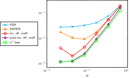
Figure 2: Convergence history under uniform mesh refinement.

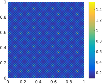
Figure 3: The scalar coefficient $A$ for the first experiment.

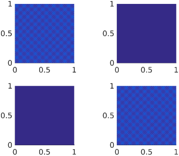
Figure 4: Matrix entries of the reconstructed localized coefficient $(A_{H}^{(\ell)})$ in the first experiment for $H=\sqrt{2}\times 2^{-6}$.

$H$	$\eta(A_{H}^{(\ell)})$	$\alpha_{H}$	$\beta_{H}$
$\sqrt{2}\times 2^{-1}$	3.2108e-02	1.9223e-01	2.0786e-01
$\sqrt{2}\times 2^{-2}$	1.1267e-02	1.9568e-01	1.9954e-01
$\sqrt{2}\times 2^{-3}$	1.4765e-02	1.9579e-01	1.9986e-01
$\sqrt{2}\times 2^{-4}$	5.3952e-01	1.8323e-01	2.1992e-01
$\sqrt{2}\times 2^{-5}$	1.7199e+00	1.6909e-01	2.3257e-01
$\sqrt{2}\times 2^{-6}$	1.5538e+01	1.4070e-01	3.0277e-01

Table 1: Values of the estimator $\eta(A_{H}^{(\ell)})$ and the bounds $\alpha_{H}$ and $\beta_{H}$ on $A_{H}$ for the first experiment. The values of the coefficient $A$ range in the interval $[\alpha,\beta]=[0.096,1.55]$.

6.2 Second experiment: Resonance effects

In this experiment we investigate so-called resonance effects of our homogenization procedure. These effects occur because, unlike in Section 5, in the present case we deal with Dirichlet boundary conditions as well as meshes that do not satisfy requirements in the spirit of Example 16. We consider a fixed mesh of width $H=\sqrt{2}\times 2^{-4}$ and the scalar coefficient

$$A(x_{1},x_{2})=\left(5+4\,\sin\left(\frac{2\pi}{\varepsilon}x_{1}\right)\sin\left(\frac{2\pi}{\varepsilon}x_{2}\right)\right)^{-1}$$

for a sequence of parameters $\varepsilon=2^{0},2^{-1},\dots,2^{-6}$. The coefficient $(A_{H}^{(\ell)})$ was computed with the same reference mesh and the same oversampling parameter as in the first experiment. Figure 5 displays the $L^{2}$ errors normalized by the $L^{2}$ error of the $L^{2}$-best approximation. On the third mesh, where $H$ and $\varepsilon$ have the same order of magnitude, the local effective coefficient leads to a larger error compared to the coarser meshes (where the coefficient is resolved by $H$) and finer meshes, where $H$ is much coarser than $\varepsilon$ and the effective coefficient is close to a constant. We observe that the values of the estimator $\eta(A_{H}^{(\ell)})$ are large in the resonance regime where also the error of the method the local effective coefficient is large. For smaller values of $\varepsilon$, the values of $\eta(A_{H}^{(\ell)})$ are close to zero, which indicates that the homogenization criterion from Remark 11 is satisfied, cf. also Remark 15.

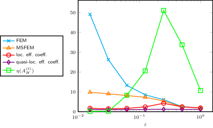
Figure 5: Resonance effect: Normalized (by $L^{2}$-best error) errors of FEM, local effective model and quasi-local effecitve model; and values of the estimator $\eta(A_{H}^{(\ell)})$.

References

• [Ada75] Robert A. Adams. Sobolev spaces, volume 65 of Pure and Applied Mathematics. Academic Press, New York-London, 1975.
• [AEEV12] Assyr Abdulle, Weinan E, Björn Engquist, and Eric Vanden-Eijnden. The heterogeneous multiscale method. Acta Numer., 21:1–87, 2012.
• [All92] G. Allaire. Homogenization and two-scale convergence. SIAM J. Math. Anal., 23(6):1482–1518, 1992.
• [All97] Grégoire Allaire. Mathematical approaches and methods. In Ulrich Hornung, editor, Homogenization and porous media, volume 6 of Interdiscip. Appl. Math., pages 225–250, 259–275. Springer, New York, 1997.
• [BL76] Jöran Bergh and Jörgen Löfström. Interpolation spaces. An introduction. Grundlehren der Mathematischen Wissenschaften, No. 223. Springer-Verlag, Berlin-New York, 1976.
• [BL11] Ivo Babuska and Robert Lipton. Optimal local approximation spaces for generalized finite element methods with application to multiscale problems. Multiscale Model. Simul., 9(1):373–406, 2011.
• [BLP78] A. Bensoussan, J.-L. Lions, and G. Papanicolaou. Asymptotic Analysis for Periodic Structures. North-Holland Publ., 1978.
• [BO10] L. Berlyand and H. Owhadi. Flux norm approach to finite dimensional homogenization approximations with non-separated scales and high contrast. Arch. Ration. Mech. Anal., 198(2):677–721, 2010.
• [Dau88] Monique Dauge. Elliptic boundary value problems on corner domains. Smoothness and asymptotics of solutions. Berlin etc.: Springer-Verlag, 1988.
• [DG75] E. De Giorgi. Sulla convergenza di alcune successioni d’integrali del tipo dell’area. Rend. Mat. (6), 8:277–294, 1975.
• [EE03] W. E and B. Engquist. The heterogeneous multiscale methods. Commun. Math. Sci., 1(1):87–132, 2003.
• [EGH13] Yalchin Efendiev, Juan Galvis, and Thomas Y. Hou. Generalized multiscale finite element methods (GMsFEM). Journal of Computational Physics, 251:116 – 135, 2013.
• [EH09] Yalchin Efendiev and Thomas Y. Hou. Multiscale finite element methods, volume 4 of Surveys and Tutorials in the Applied Mathematical Sciences. Springer, New York, 2009.
• [GGS12] L. Grasedyck, I. Greff, and S. Sauter. The AL basis for the solution of elliptic problems in heterogeneous media. Multiscale Model. Simul., 10(1):245–258, 2012.
• [GH08] I. Greff and W. Hackbusch. Numerical method for elliptic multiscale problems. J. Numer. Math., 16(2):119–138, 2008.
• [GP15] D. Gallistl and D. Peterseim. Stable multiscale Petrov-Galerkin finite element method for high frequency acoustic scattering. Comput. Methods Appl. Mech. Eng., 295:1–17, 2015.
• [GP17] D. Gallistl and D. Peterseim. Numerical stochastic homogenization by quasilocal effective diffusion tensors. ArXiv e-prints, 1702.08858, 2017.
• [Gri85] P. Grisvard. Elliptic problems in nonsmooth domains, volume 24 of Monographs and Studies in Mathematics. Pitman (Advanced Publishing Program), Boston, MA, 1985.
• [Hac15] Wolfgang Hackbusch. Hierarchical matrices: algorithms and analysis. Springer, Berlin, 2015.
• [HFMQ98] T. J. R. Hughes, G. R. Feijóo, L. Mazzei, and J.-B. Quincy. The variational multiscale method–a paradigm for computational mechanics. Comput. Meth. Appl. Mech. Engrg., 166(1-2):3–24, 1998.
• [HMP15] Patrick Henning, Philipp Morgenstern, and Daniel Peterseim. Multiscale partition of unity. In M. Griebel and M. A. Schweitzer, editors, Meshfree Methods for Partial Differential Equations VII, volume 100 of Lect. Notes Comput. Sci. Eng., pages 185–204. Springer International Publishing, 2015.
• [HP13] P. Henning and D. Peterseim. Oversampling for the multiscale finite element method. Multiscale Model. Simul., 11(4):1149–1175, 2013.
• [HS07] T. J. R. Hughes and G. Sangalli. Variational multiscale analysis: the fine-scale Green’s function, projection, optimization, localization, and stabilized methods. SIAM J. Numer. Anal., 45(2):539–557, 2007.
• [HW97] Thomas Y. Hou and Xiao-Hui Wu. A multiscale finite element method for elliptic problems in composite materials and porous media. J. Comput. Phys., 134(1):169–189, 1997.
• [KPY16] R. Kornhuber, D. Peterseim, and H. Yserentant. An analysis of a class of variational multiscale methods based on subspace decomposition. ArXiv e-prints, 1608.04081, 2016.
• [KY16] Ralf Kornhuber and Harry Yserentant. Numerical homogenization of elliptic multiscale problems by subspace decomposition. Multiscale Modeling & Simulation, 14(3):1017–1036, 2016.
• [Mål11] A. Målqvist. Multiscale methods for elliptic problems. Multiscale Model. Simul., 9(3):1064–1086, 2011.
• [Mel02] Jens M. Melenk. $hp$-finite element methods for singular perturbations, volume 1796 of Lecture Notes in Mathematics. Springer-Verlag, Berlin, 2002.
• [MP14] A. Målqvist and D. Peterseim. Localization of elliptic multiscale problems. Math. Comp., 83(290):2583–2603, 2014.
• [MS02] Matache, Ana-Maria and Schwab, Christoph. Two-scale fem for homogenization problems. ESAIM: M2AN, 36(4):537–572, 2002.
• [MT78] F. Murat and L. Tartar. H-convergence. Séminaire d’Analyse Fonctionnelle et Numérique de l’Université d’Alger, 1978.
• [Ngu89] G. Nguetseng. A general convergence result for a functional related to the theory of homogenization. SIAM J. Math. Anal., 20(3):608–623, 1989.
• [Owh17] Houman Owhadi. Multigrid with rough coefficients and multiresolution operator decomposition from hierarchical information games. SIAM Review, 59(1):99–149, 2017.
• [OZ07] Houman Owhadi and Lei Zhang. Metric-based upscaling. Comm. Pure Appl. Math., 60(5):675–723, 2007.
• [OZB14] Houman Owhadi, Lei Zhang, and Leonid Berlyand. Polyharmonic homogenization, rough polyharmonic splines and sparse super-localization. ESAIM Math. Model. Numer. Anal., 48(2):517–552, 2014.
• [Pet16] D. Peterseim. Variational multiscale stabilization and the exponential decay of fine-scale correctors. In G. R. Barrenechea, F. Brezzi, A. Cangiani, and E. H. Georgoulis, editors, Building Bridges: Connections and Challenges in Modern Approaches to Numerical Partial Differential Equations, volume 114 of Lect. Notes Comput. Sci. Eng., pages 341–367. Springer, 2016.
• [Spa68] S. Spagnolo. Sulla convergenza di soluzioni di equazioni paraboliche ed ellittiche. Ann. Scuola Norm. Sup. Pisa (3) 22 (1968), 571-597; errata, ibid. (3), 22:673, 1968.
• [WS15] Monika Weymuth and Stefan Sauter. An adaptive local (AL) basis for elliptic problems with complicated discontinuous coefficients. In PAMM Proc. Appl. Math. Mech., volume 15, pages 605–606, 2015.