New efficient substepping methods for exponential timestepping.

Abstract

Exponential integrators are time stepping schemes which exactly solve the linear part of a semilinear ODE system. This class of schemes requires the approximation of a matrix exponential in every step, and one successful modern method is the Krylov subspace projection method. We investigate the effect of breaking down a single timestep into arbitrary multiple substeps, recycling the Krylov subspace to minimise costs. For these recyling based schemes we analyse the local error, investigate them numerically and show they can be applied to a large system with $10^{6}$ unknowns. We also propose a new second order integrator that is found using the extra information from the substeps to form a corrector to increase the overall order of the scheme. This scheme is seen to compare favourably with other order two integrators.

1 Introduction

We consider the numerical integration of a large system of semilinear ODEs of the form

$$\frac{du}{dt}=Lu+F(t,u(t))\qquad u(0)=u_{0},\quad t\in[0,\infty)$$ (1)

with $u,F(t,u(t))\in\mathbb{R}^{N}$ and $L\in\mathbb{R}^{N\times N}$ a matrix. Equation (1) arises, for example, from the spatial discretisation of reaction-diffusion-advection equations. An increasingly popular method for approximating the solution of semlinar ODE systems such as (1) are exponential integrators. These are a class of schemes which approximate (1) by exactly solving the linear part and are characterised by requiring the evaluation or approximation of a matrix exponential function of $L$ at each timestep. A major class of exponential integrators are the multistep Exponential Time Differencing (ETD) schemes, first developed in [1], other classes include the Exponential Euler Midpoint method [2] and Rosenbrock type methods [3, 4]. For an overview of exponential integrators see [5, 6] and other useful references can be found in [7].

Approximating the matrix exponential and functions of it (like $\varphi-$functions in (3) below) is a notoriously difficult problem [8]. A classical technique is Padé approximation, which is only efficient for small matrices. Modern methods range from Taylor series methods making sophisticated use of scaling and squaring for efficiency, [9], to approximation with Faber or Chebyschev polynomials [10], [5] §4.1, interpolation on Leja points [11, 12, 13, 14, 15], to Krylov subspace projection techniques [16, 17, 18, 19, 20] which is what we consider here.

Our schemes are based on the standard exponential integrator ETD1, which can be written as

$$u_{n+1}^{etd}=u_{n}^{etd}+\Delta t\varphi_{1}(\Delta tL)\left(Lu_{n}^{etd}+F_{n}^{etd}\right).$$ (2)

where $\varphi_{1}(\Delta tL)$ is defined shortly; $u_{n}^{etd}\approx u(t_{n})$ at discrete times $t_{n}=n\Delta t$ for fixed $\Delta t>0$, $F_{n}^{etd}\equiv F(t_{n},u_{n}^{etd})$0 and $n\in\mathbb{N}$. ETD1 is globally first order, and is derived from (1) by variation of constants and approximating $F(t,u(t))$ by the constant $F_{n}^{etd}$ over one timestep. See for example [5, 6, 7, 21] for more detail. It is useful to introduce the additional notation

$$g(t)\equiv Lu(t)+F(t,u(t))\quad\text{and}\quad g_{n}^{etd}\equiv Lu_{n}^{etd}+F(t_{n},u_{n}^{etd}).$$

The function $\varphi_{1}$ is part of a family of matrix exponential functions defined by $\varphi_{0}(z)=e^{z}$, $\varphi_{1}(z)=z^{-1}\left(e^{z}-I\right),$ and in general

$$\varphi_{k+1}(z)=z^{-1}\left(\varphi_{k+1}-\frac{I}{k!}\right),$$ (3)

where $I$ is the identity matrix. These $\varphi-$functions appear in all exponential integrator schemes; see [19]. In particular we use $\varphi_{1}$, and for brevity we introduce the following notation

$$p_{\tau}\equiv\tau\varphi_{1}(\tau L).$$ (4)

We can then re-write (2) as

$$u_{n+1}^{etd}=u_{n}^{etd}+p_{\Delta t}g_{n}^{etd}$$ (5)

We consider the Krylov projection method for approximating terms like $p_{\Delta t}g_{n}^{etd}$ in (2). In the Krylov method, this term is approximated on a Krylov subspace defined by the vector $g_{n}$ and the matrix $L$. Typically the subspace is recomputed, in the form of a matrix of basis vectors $V_{m}$, every time the solution vector, $u_{n}$ in (2), is updated (and thus also $g_{n}$). This is done using a call to the Arnoldi algorithm [16], and is often the most expensive part of each step. It is possible to ‘recycle’ this matrix at least once, as demonstrated in [22] for the exponential Euler method (EEM) (see [5] and (51)). In this paper we investigate this possibility further and use it to construct new methods based on ETD1 and in A we show how to construct the general recycling method for EEM.

We examine the effect of splitting the single step of (2) of length $\Delta t$ in to $S$ substeps of length $\delta t=\frac{\Delta t}{S}$, through which the Krylov subspace and matrices are recycled. By deriving expressions for the local error, we show that the scheme remains locally second order for any number $S$ of substeps, and that the leading term of the local error decreases. This gives a method based on recyling the Krylov subspace for $S$ substeps. We then obtain a second method using the extra information from the substeps to form a corrector to increase the overall order of the scheme.

The paper is arranged as follows. In Section 2 we describe the Krylov subspace projection method for approximating the action of $\varphi-$functions on vectors. In Section 3 we describe the concept of recycling the Krylov subspace across substeps in order to increase the accuracy of the ETD1 based scheme, and show that the leading term of the local error of the scheme decreases as the number of substeps uses increases. We then prove a lemma to express the local error expression at arbitrary order. With this information about the local error expansion, and the extra information from the substeps taken, it is possible to construct correctors for the scheme the increase the accuracy and local order of the scheme. We demonstrate one simple such corrector in Section 4. Numerical examples demonstrating the effectiveness of this scheme are presented in Section 5.

2 The Krylov Subspace Projection Method and ETD1

We describe the Krylov subspace projection method for approximating $\varphi_{1}(\Delta tL)$ in (2). We motivate this by showing how the leading powers of $\Delta tL$ in $L$ are captured by the subspace. The series definition of $\varphi_{1}(\Delta tL)$ is,

$$\varphi_{1}(\Delta tL)\equiv\sum_{k=0}^{\infty}{\frac{(\Delta tL)^{k}}{(k+1)!}}.$$ (6)

The challenge in applying the scheme (2) is to efficiently compute, or approximate, the action of $\varphi_{1}$ on the vector $g_{n}^{etd}$. The sum in (6) is useful in motivating a polynomial Krylov subspace approximation. The $m$-dimensional Krylov subspace for the matrix $L$ and vector $g\in\mathbb{R}^{N}$ is defined by:

$$\mathcal{K}_{m}(L,g)=\mbox{span}\{g,Lg,\ldots,L^{m-1}g\}.$$ (7)

Approximating sum in (6) by the first $m$ terms is equivalent to approximation in the subspace $\mathcal{K}_{m}(L,g_{n}^{etd})$ in (7). We now review some simple results about the general subspace $\mathcal{K}_{m}(L,g)$, with arbitrary vector $g$, before using the results with $g=g_{n}^{etd}$ to demonstrate how they are used in the evaluation of (2).
The Arnoldi algorithm (see e.g. [19], [16]) is used to produce an orthonormal basis $\{v_{1},\ldots,v_{n}\}$ for the space $\mathcal{K}_{m}(L,g)$ such that

$$\mbox{span}\{v_{1},v_{2},\ldots,v_{m}\}=\mbox{span}\{g,Lg,\ldots,L^{m-1}g\}.$$ (8)

It produces two matrices $V_{m}\in\mathbb{R}^{N\times m}$, whose columns are the $v_{k}$, and an upper Hessenburg matrix $H_{m}\in\mathbb{R}^{m\times m}$. The matrices $L$,$H_{m}$ and $V_{m}$ are related by

$$L=V_{m}^{T}H_{m}V^{T},$$ (9)

see, for example, equation (2) in [16], of which (9) is a consequence. From (9) it follows that,

$$V_{m}H_{m}V_{m}^{T}=V_{m}V_{m}^{T}LV_{m}V_{m}^{T}.$$ (10)

For any $x\in\mathcal{K}_{m}(L,g)$,

$$V_{m}V_{m}^{T}x=x,$$

since $V_{m}V_{m}^{T}x$ represents the orthogonal projection into the space $\mathcal{K}_{m}(L,g)$. Therefore, since $L^{k}g\in\mathcal{K}_{m}(L,g_{n})$, we also have that

$$V_{m}V_{m}^{T}L^{k}g=L^{k}g\qquad\text{for }\qquad 0\leq k\leq m-1$$

We now consider the relationship between $L^{k}g$ and $V_{m}H_{m}^{k}V_{m}^{T}g$.

Lemma 2.1.

Assume $0\leq k\leq m-1$. Then for $H_{m}$, $V_{m}$ corresponding to the Krylov subspace $\mathcal{K}(L,g)$,

$$V_{m}H_{m}^{k}V_{m}^{T}g=L^{k}g.$$ (11)

Proof.

We have that $V_{m}H_{m}^{k}V_{m}^{T}=(V_{m}H_{m}V_{m}^{T})^{k}$ since $V_{m}^{T}V_{m}=I$. Let $\pi\equiv V_{m}V_{m}^{T}$, the projector into $\mathcal{K}(L,g)$, so that (10) can be more briefly written $V_{m}H_{m}V_{m}^{T}=\pi L\pi$. Then by (10) we find

$$V_{m}H_{m}^{k}V_{m}^{T}g=(\pi L\pi)^{k}g=(\pi L\pi)^{k-1}\pi L\pi g=(\pi L\pi)^{k-1}Lg=\ldots=L^{k}g.$$ (12)

∎

Now consider using the vector $g=g_{n}^{etd}$, to generate the subspace $\mathcal{K}_{m}(L,g_{n}^{etd})$, and the corresponding matrices $H_{m}$, $V_{m}$, by the Arnoldi algorithm. By Lemma 11 we have that, up to $k=m$,

$$V_{m}H_{m}^{k}V_{m}^{T}g_{n}^{etd}=L^{k}g_{n}^{etd}.$$

Thus, inserting the approximation $L\approx V_{m}H_{m}^{k}V_{m}^{T}$ in $\varphi_{1}(\Delta tL)$ the first $m$ terms are correctly approximated. The Krylov approximation is then

$$\begin{split}\Delta t\varphi_{1}(\Delta tL)g_{n}\approx\Delta t\varphi_{1}(\Delta tV_{m}H_{m}V_{m}^{T})g_{n}&=\Delta tV_{m}\varphi_{1}(\Delta tH_{m})V_{m}^{T}g_{n}\\ &=||g_{n}||\Delta tV_{m}\varphi_{1}(\Delta tH_{m})e_{1}.\end{split}$$ (13)

Let us introduce a shorthand notation for the Krylov approximation of the $\varphi-$function. Analogous to (4), for $\tau\in\mathbb{R}$ let

$$\tilde{p}_{\tau}\equiv\tau V_{m}\varphi_{1}(\tau H_{m})V_{m}^{T}\approx p_{\tau}.$$ (14)

Using (13) and (14) we then approximate (5) by $u_{n+1}^{etd}=u_{n}^{etd}+\tilde{p}_{\Delta t}g_{n}^{etd}.$ The key here is that the $\varphi_{1}(\Delta tH_{m})$ now needs to be evaluated instead of $\varphi_{1}(\Delta tL)$. $m$ is chosen such that $m\ll N$, and a classical method such as a rational Padé is used for $\varphi_{1}(\Delta tH_{m})$, which would be prohibitively expensive for $\varphi_{1}(\Delta tL)$ for large $N$.
One step of the ETD1 scheme (2), under the approximation $\varphi_{1}(\Delta tL)\approx V_{m}\varphi_{1}(\Delta tH_{m})V_{m}^{t}$, becomes

$$\begin{split}u_{n+1}&=u_{n}+\Delta tV_{m}\varphi_{1}(\Delta tH)V_{m}^{T}g_{n}\\ &=||g_{n}||\Delta tV_{m}\varphi_{1}(\Delta tH)e_{1},\end{split}$$ (15)

where $e_{1}$ is the first basis vector in $\mathbb{R}^{m}$.

3 Recycling the Krylov subspace

In the Krylov subspace projection method described in §2, the subspace $\mathcal{K}_{m}(L,g_{n})$ and thus the matrices $H_{m}$ and $V_{m}$ depend on $g_{n}$. At each step it is understood that a new subspace must be formed, and $H_{m}$, $V_{m}$ be re-generated by the Arnoldi method, since $g_{n}$ changes. In [22] it is demonstrated that splitting the timestep into two substeps, and recycling $H_{m}$ and $V_{m}$, i.e. recycling the Krylov subspace, can be viable (in that it does not decrease the local order of the scheme, and apparently decreases the error). We expand on this concept with a more detailed analysis of the effect of this kind of recycled substepping applied to the locally second order ETD1 scheme (2) (EEM is considered in A). We replace a single step of length $\Delta t$ of (15) with $S$ substeps of length $\delta t$, such that $\Delta t=S\delta t$. We denote the approximations used in this scheme analogously to the notation for ETD1 earlier, without the $etd$ superscript, and introduce the following notation to keep track of substeps

$$u_{n+\frac{j}{S}}\approx u(t_{n}+j\delta t)\qquad\text{and}\qquad F_{n+\frac{j-1}{S}}\approx F(t_{n}+j\delta t,u_{n+\frac{j}{S}}).$$

For $j=1$ we calculate $H_{m}$, $V_{m}$, from $g_{n}$,

$$u_{n+\frac{1}{S}}=u_{n}+\delta tV_{m}\varphi_{1}(\delta tH_{m})V_{m}^{T}g_{n},$$ (16)

and for the remaining $S-1$ steps,

$$u_{n+\frac{j}{S}}=u_{n+\frac{j-1}{S}}+\delta tV_{m}\varphi_{1}(\delta tH_{m})V_{m}^{T}\left(Lu_{n+\frac{j-1}{S}}+F_{n+\frac{j-1}{S}}\right)\mbox{, }1<j\leq S,$$ (17)

where the matrices $H_{m}$ and $V_{m}$ are not re-calculated for any substep, $j>1$. We call substeps of the form (17) ‘recycled steps’ and substeps of the form (16) ‘initial steps’. The approximation to $u(t_{n}+\Delta t)$ at the end of the step of length $\Delta t$ is then given by

$$u_{n+1}=u_{n+\frac{S-1}{S}}+\delta tV_{m}\varphi_{1}(\delta tH_{m})V_{m}^{T}\left(Lu_{n+\frac{S-1}{S}}+F_{n+\frac{S-1}{S}}\right).$$ (18)

The recycling steps (16), (17) can be succinctly expressed using the definition of $\tilde{p}_{\tau}$;

$$u_{n+\frac{1}{S}}=u_{n}+\tilde{p}_{\delta t}g_{n},$$ (19)

$$u_{n+\frac{j}{S}}=u_{n+\frac{j-1}{S}}+\tilde{p}_{\delta t}\left(Lu_{n+\frac{j-1}{S}}+F_{n+\frac{j-1}{S}}\right)\mbox{, }1<j\leq S.$$ (20)

3.1 The local error of the recycling scheme

We now derive an expression for the local error of the scheme defined by (16), (17) and prove that the leading term decreases with the number of substeps $S$. We use the local error assumption that $u_{n}=u(t_{n})$ and make an assumption about the accuracy of the initial Krylov approximation with respect to the error of the scheme. Let the error in the polynomial Krylov approximation over a single step (including the error from the approximation of $\varphi_{1}(\tau H_{m})$ using, e.g. Padé approximation), with subspace dimension of size $m$, be given by $\mathcal{E}_{n+1}^{m}$, so that,

$$\tilde{p}_{\tau}g_{n}=p_{\tau}g_{n}+\mathcal{E}_{n+1}^{m}.$$ (21)

Assumption 3.1.

The Krylov approximation error $\mathcal{E}_{n+1}^{m}$ is much less than the error of ETD1, and thus does not affect the leading term of the local error of ETD1.

Bounds on $\mathcal{E}_{n+1}^{m}$ can be found in for example [17, 16]. Practically, we can always reduce $\Delta t$ or increase $m$ until Assumption 3.1 is satisfied.
For the local error of the recycling scheme, the following result will be used.

Lemma 3.2.

For any $\tau_{1},\tau_{2}\in\mathbb{R}$, and any vector $v\in\mathbb{R}^{N}$,

$$p_{\tau_{1}}v+p_{\tau_{2}}\left(Lp_{\tau_{1}}v+v\right)=p_{\tau_{1}+\tau_{2}}v,$$

and the same relation holds for the Krylov approximations, that is,

$$\tilde{p}_{\tau_{1}}v+\tilde{p}_{\tau_{2}}\left(L\tilde{p}_{\tau_{1}}v+v\right)=\tilde{p}_{\tau_{1}+\tau_{2}}v.$$

Proof.

We prove the second equation. The first can be proved using an almost identical argument, replacing $\tilde{p}_{\tau}$ by $p_{\tau}$ where appropriate.
By the definitions of $\tilde{p}_{\tau}$, and $\varphi_{1}$, i.e. $\tilde{p}_{\tau}=V\varphi_{1}(\tau H_{m})V_{m}^{T}=V_{m}H_{m}^{-1}\left(e^{\tau_{2}H_{m}}-I\right)V_{m}^{T}$ we have

$$\tilde{p}_{\tau_{2}}\left(L\tilde{p}_{\tau_{1}}v+v\right)=V_{m}H_{m}^{-1}\left(e^{\tau_{2}H_{m}}-I\right)V_{m}^{T}\left(LV_{m}H_{m}^{-1}\left(e^{\tau_{1}H_{m}}-I\right)V_{m}^{T}+I\right)v.$$

By (9) this becomes $\tilde{p}_{\tau_{2}}\left(L\tilde{p}_{\tau_{1}}v+v\right)=V_{m}H_{m}^{-1}\left(e^{(\tau_{2}+\tau_{1})H_{m}}-e^{\tau_{1}H_{m}}\right)V_{m}^{T}v.$ Now using the definition of $\tilde{p}_{\tau_{1}}$,

$$\begin{split}&\tilde{p}_{\tau_{1}}v+\tilde{p}_{\tau_{2}}\left(L\tilde{p}_{\tau_{1}}v+v\right)\\ &=V_{m}H_{m}^{-1}\left(e^{\tau_{1}H_{m}}-I\right)V_{m}^{T}v+V_{m}H_{m}^{-1}\left(e^{(\tau_{2}+\tau_{1})H_{m}}-e^{\tau_{1}H_{m}}\right)V_{m}^{T}v\\ &=V_{m}H_{m}^{-1}\left(e^{(\tau_{2}+\tau_{1})H_{m}}-I\right)V_{m}^{T}v,\end{split}$$

which is $\tilde{p}_{\tau_{1}+\tau_{2}}v$ as desired. ∎

Without recycling substeps, a single ETD1 step (2) of length $\Delta t$, using the polynomial Krylov approximation, would be:

$$u_{n+1}^{etd}=u_{n}^{etd}+\tilde{p}_{\Delta t}g_{n}^{etd}.$$ (22)

To examine the local error we compare $u_{n+1}^{etd}$ with the $u_{n+1}$ obtained after some number $S$ of recycled substeps. We can write

$$u_{n+1}=u_{n}+\tilde{p}_{\Delta t}g_{n}+R_{n+1}^{S},$$

where $R_{n+1}^{S}$ represents the deviation from (22) over one step. Then we have:

Lemma 3.3.

The approximation $u_{n+\frac{j}{S}}$ produced by $j$ substeps of the recycling scheme (19), (20), satisfies

$$u_{n+\frac{j}{S}}=u_{n}+\tilde{p}_{j\delta t}g_{n}+R_{n+\frac{j}{S}}^{S},$$ (23)

with

$$R_{n+\frac{j}{S}}^{S}=\sum_{k=1}^{j}{(I+\tilde{p}_{\delta t}L)^{j-k}\tilde{p}_{\delta t}(F_{n+\frac{k-1}{S}}-F_{n})}.$$ (24)

Proof.

By induction. For $j=1$, $u_{n+\frac{1}{S}}$ is given by (19) and $R_{n+\frac{1}{S}}^{S}=0$. Equation (24) gives $R_{n+\frac{1}{S}}^{S}=\tilde{p}_{\delta t}(F_{n+\frac{0}{S}}-F_{n})=0$ as required.
Assume now (23) holds for some $j\geq 1$. Then $u_{n+\frac{j+1}{S}}$ is obtained by a step of (20). Using (23) we find,

$$u_{n+\frac{j+1}{S}}=u_{n+\frac{j}{S}}+\tilde{p}_{\delta t}\left(Lu_{n}+L\tilde{p}_{j\delta t}g_{n}+LR_{n+\frac{j}{S}}^{S}+F_{n+\frac{j}{S}}\right),$$

and since $Lu_{n}=g_{n}-F(t_{n},u(t_{n}))$, by the induction hypothesis,

$$\begin{split}u_{n+\frac{j+1}{S}}&=u_{n+\frac{j}{S}}+\tilde{p}_{\delta t}\left(g_{n}+L\tilde{p}_{\delta t}g_{n}+LR_{n+\frac{j}{S}}^{S}+F_{n+\frac{j}{S}}-F(t_{n},u(t_{n}))\right)\\ &=u_{n+\frac{j}{S}}+\tilde{p}_{\delta t}\left(g_{n}+L\tilde{p}_{\delta t}g_{n}\right)+\tilde{p}_{\delta t}LR_{n+\frac{j}{S}}^{S}+\tilde{p}_{\delta t}(F_{n+\frac{j}{S}}-F_{n})\\ &=u_{n}+\tilde{p}_{j\delta t}g_{n}+\tilde{p}_{\delta t}\left(g_{n}+L\tilde{p}_{\delta t}g_{n}\right)+(I+\tilde{p}_{\delta t}L)R_{n+\frac{j}{S}}^{S}+\tilde{p}_{\delta t}(F_{n+\frac{j}{S}}-F_{n}).\end{split}$$

Thus by Lemma 3.2 we have that,

$$u_{n+\frac{j+1}{S}}=u_{n}+\tilde{p}_{(j+1)\delta t}g_{n}+\tilde{p}_{\delta t}(F_{n+\frac{j}{S}}-F_{n})+(I+\tilde{p}_{\delta t}L)R_{n+\frac{j}{S}}^{S}.$$

To complete the proof we need to show:

$$R_{n+\frac{j+1}{S}}^{S}=\tilde{p}_{\delta t}(F_{n+\frac{j}{S}}-F_{n})+(I+\tilde{p}_{\delta t}L)R_{n+\frac{j}{S}}^{S}.$$ (25)

By the induction hypothesis that (24) holds for $j$,

$$\begin{split}&\tilde{p}_{\delta t}(F_{n+\frac{j}{S}}-F_{n})+(I+\tilde{p}_{\delta t}L)R_{n+\frac{j}{S}}^{S}\\ &=\tilde{p}_{\delta t}(F_{n+\frac{j}{S}}-F_{n})+(I+\tilde{p}_{\delta t}L)\sum_{k=1}^{j}{(I+\tilde{p}_{\delta t}L)^{j-k}\tilde{p}_{\delta t}(F_{n+\frac{j-1}{S}}-F_{n})}\\ &=\sum_{k=1}^{j+1}{(I+\tilde{p}_{\delta t}L)^{j+1-k}\tilde{p}_{\delta t}(F_{n+\frac{k-1}{S}}-F_{n})}=R_{n+\frac{j+1}{S}}^{S}.\end{split}$$ (26)

Hence the lemma is proved. ∎

Using (23) we now express the leading order term of the local error in terms of $S$. First we examine the leading order term of $R_{n+1}^{S}$.

Lemma 3.4.

The term $R_{n+\frac{j}{S}}^{S}$ in Lemma 24, when expanded in powers of $\Delta t$, satisfies

$$R_{n+\frac{j}{S}}^{S}=\frac{j(j-1)}{2}\delta t^{2}V_{m}V_{m}^{T}\frac{dF(t_{n},u_{n})}{dt}+O(\Delta t^{3}).$$ (27)

Proof.

By induction. Since $(F_{n+\frac{0}{S}}-F_{n})=0$, then, $R_{n+\frac{1}{S}}^{S}=0$, so that (27) is true for $j=1$. Now assume the result holds for some $j$. Then we can express the term $F_{n+\frac{j}{S}}$ follows:

$$\begin{split}F(t_{n+\frac{j}{S}},u_{n+\frac{j}{S}})&=F(t_{n+\frac{j}{S}},u_{n}+(j\delta tg_{n}+O(\delta t^{2})))\\ &=F(t_{n},u_{n})+j\delta t\frac{\partial F}{\partial t}(t_{n},u_{n})+j\delta t\frac{\partial F}{\partial u}(t_{n},u_{n})g_{n}+O(\delta t^{2})\\ &=F(t_{n},u_{n})+j\delta t\frac{dF}{dt}(t_{n},u_{n})+O(\delta t^{2}).\end{split}$$

We thus have that

$$(F_{n+\frac{j}{S}}-F_{n})=j\delta t\frac{dF}{dt}(t_{n},u_{n})+O(\delta t^{2}).$$ (28)

We then insert (28) into the inductive expression (27) for $R_{n+\frac{j}{S}}^{S}$ and use the expansion $\tilde{p}_{\delta t}=\delta tV_{m}V_{m}^{T}+O(\delta t^{2})$ to get

$$R_{n+\frac{j+1}{S}}^{S}=\delta tV_{m}V_{m}^{T}j\delta t\frac{dF}{dt}(t_{n},u_{n})+(I+\delta tV_{m}V_{m}^{T}L)R_{n+\frac{j}{S}}^{S}+O(\delta t^{3}).$$

Using the induction assumption (27),

$$R_{n+\frac{j+1}{S}}^{S}=\delta tV_{m}V_{m}^{T}j\delta t\frac{dF}{dt}(t_{n},u_{n})+\frac{j(j-1)}{2}\delta t^{2}V_{m}V_{m}^{T}\frac{dF(t_{n},u_{n})}{dt}+O(\Delta t^{3}).$$

Noting that $\Delta t=S\delta t$ we can write $O(\Delta t^{3})$ as $O(\delta t^{3})$. Collecting terms we have,

$$R_{n+\frac{j+1}{S}}^{S}=\left(\frac{j(j-1)}{2}+j\right)\delta t^{2}V_{m}V_{m}^{T}\frac{dF(t_{n},u_{n})}{dt}+O(\Delta t^{3}).$$

The lemma follows since $\frac{j(j-1)}{2}+j=\frac{j(j+1)}{2}$. ∎

The leading local error term of the ETD1 scheme without substeps is well known to be $\frac{\Delta t^{2}}{2}\frac{dF(t)}{dt}$ (see [23]), so that we can finally recover the leading term from Lemma 24.

Corollary 3.5.

The leading term of the recycling scheme after $j$ steps is

$$u_{n+\frac{j}{S}}=u_{n}+j\delta tg_{n}+\frac{j^{2}\delta t^{2}}{2}Lg_{n}+\frac{j(j-1)}{2}\delta t^{2}V_{m}V_{m}^{T}\frac{dF(t_{n},u_{n})}{dt}+O(\delta t^{3}).$$ (29)

Corollary 3.6.

The local error $u(t_{n}+\Delta t)-u_{n+1}$ of an ETD1 Krylov recycling scheme is second order for any number $S$ of recycled substeps. Moreover, the local error after $j$ recycled steps is

$$u(t_{n}+j\delta t)-u_{n+\frac{j}{S}}=\frac{(j\delta t)^{2}}{2}\left(I-\frac{j-1}{j}V_{m}V_{m}^{T}\right)\frac{df(t)}{dt}+O(\delta t^{3}).$$

In particular

$$u(t_{n}+\Delta t)-u_{n+1}=\frac{\delta t^{2}}{2}\left(S^{2}-S(S-1)V_{m}V_{m}^{T}\right)\frac{df(t)}{dt}+O(\delta t^{2}),$$ (30)

or in terms of $\Delta t$

$$u(t_{n}+\Delta t)-u_{n+1}=\frac{\Delta t^{2}}{2}\left(I-\frac{S-1}{S}V_{m}V_{m}^{T}\right)\frac{df(t)}{dt}+O(\Delta t^{2}).$$ (31)

It is interesting to compare (31) with the leading term of the local error of regular ETD1, $\frac{\Delta t^{2}}{2}\frac{df}{dt}$. Since $V_{m}V_{m}^{T}$ is the orthogonal projector into $\mathcal{K}$, then we can see that the $\frac{\Delta t^{2}}{2}\frac{S-1}{S}V_{m}V_{m}^{T}\frac{df(t)}{dt}$ part in (31) is the projection of the ETD1 error into $\mathcal{K}$, multiplied by a factor $\frac{S-1}{S}\leq 1$. Thus, in the leading term, according to (31), the recycling scheme reduces the error of ETD1 by effectively eliminating the part of the error which lives in $\mathcal{K}$. In the limit $S\rightarrow\infty$, the entirety of the error in $\mathcal{K}$ will be eliminated. The effectiveness of the recycling scheme therefore depends on how much of $\frac{df(t)}{dt}$ can be found in $\mathcal{K}$.
Corollary 31 shows that using $S>1$ recycled substeps is advantageous over the basic ETD1 scheme, in the sense of reducing the magnitude of the leading local error term, whenever

$$\left|\left|\left(I-\frac{S-1}{S}V_{m}V_{m}^{T}\right)\frac{df(t)}{dt}\right|\right|<\left|\left|\frac{df(t)}{dt}\right|\right|,$$ (32)

where $\left|\left|\cdot\right|\right|$ is a given vector norm. We show in Lemma 3.8 that increasing $S$ will decrease the Euclidean norm $||\cdot||_{2}$ of the leading term of the local error. First we require a result on $V_{m}V_{m}^{T}$, the projector into the Krylov Supspace $\mathcal{K}$.

Remark 3.7.

Let $x\neq 0$ be a vector such that $V_{m}V_{m}^{T}x\neq 0$, then for $\alpha\in\mathbb{R}$

$$\left|\left|\left(I-\alpha V_{m}V_{m}^{T}\right)x\right|\right|_{2}^{2}=\left|\left|x\right|\right|_{2}^{2}+[(1-\alpha)^{2}-1]\left|\left|V_{m}V_{m}^{T}x\right|\right|_{2}^{2}.$$ (33)

Proof.

An elementary result for orthogonal projectors (see, e.g. [24]) is that

$$\left|\left|x\right|\right|_{2}^{2}=\left|\left|V_{m}V_{m}^{T}x\right|\right|_{2}^{2}+\left|\left|(I-V_{m}V_{m}^{T})x\right|\right|_{2}^{2},$$ (34)

which follows from $V_{m}V_{m}^{T}x\bot(I-V_{m}V_{m}^{T})x$ (the orthogonality of $V_{m}V_{m}^{T}x$ and $(I-V_{m}V_{m}^{T})x$) and the definition of the Euclidean norm. Equation (33) is a generalisation of (34) as can be shown as follows.
Write $x-\alpha V_{m}V_{m}^{T}x=(I-V_{m}V_{m}^{T})x+(1-\alpha)V_{m}V_{m}^{T}x$, and then, noting that $(I-V_{m}V_{m}^{T})x\bot(1-\alpha)V_{m}V_{m}^{T}x$, we see that

$$\left|\left|x-\alpha V_{m}V_{m}^{T}x\right|\right|_{2}^{2}=\left|\left|(I-V_{m}V_{m}^{T})x\right|\right|_{2}^{2}+(1-\alpha)^{2}\left|\left|V_{m}V_{m}^{T}x\right|\right|_{2}^{2}.$$

Using (34) to substitute for $\left|\left|(I-V_{m}V_{m}^{T})x\right|\right|_{2}^{2}$ yields (33). ∎

Lemma 3.8.

Assume $\frac{df(t)}{dt}\neq 0$ and $V_{m}V_{m}^{T}\frac{df(t)}{dt}\neq 0$. Let $E_{S_{1}}$ be the local error using the recycling scheme over a timestep of length $\Delta t$ with $S_{1}\geq 1$ substeps, and $E_{S_{2}}$ the local error with $S_{2}$ substeps with $S_{2}>S_{1}$. Then,

$$\left|\left|E_{S_{2}}\right|\right|_{2}<\left|\left|E_{S_{1}}\right|\right|_{2}.$$

Proof.

The local errors $E_{S_{k}}$, $k=1,2$ are given in Corollary 31. Let $\frac{S_{k}-1}{S_{k}}\equiv\beta_{k}$, $k=1,2$. We need to show that

$$\left|\left|\left(I-\beta_{2}V_{m}V_{m}^{T}\right)\frac{df(t)}{dt}\right|\right|_{2}<\left|\left|\left(I-\beta_{1}V_{m}V_{m}^{T}\right)\frac{df(t)}{dt}\right|\right|_{2}.$$

Let $x\equiv\left(I-\beta_{1}V_{m}V_{m}^{T}\right)\frac{df(t)}{dt}$, then $\left(I-\beta_{2}V_{m}V_{m}^{T}\right)\frac{df(t)}{dt}=x-\left(\frac{\beta_{1}-\beta_{2}}{\beta_{1}-1}\right)V_{m}V_{m}^{T}x$ (showing this involves using $V_{m}V_{m}^{T}V_{m}V_{m}^{T}=V_{m}V_{m}^{T}$). Letting $\gamma\equiv\frac{\beta_{1}-\beta_{2}}{\beta_{1}-1}$, we then need to show

$$\left|\left|\left(I-\gamma V_{m}V_{m}^{T}\right)x\right|\right|_{2}<\left|\left|x\right|\right|_{2}.$$ (35)

Note that we have that $V_{m}V_{m}^{T}x\neq 0$ from the assumptions. This is because,

$$V_{m}V_{m}^{T}x=\left(V_{m}V_{m}^{T}-\beta_{1}V_{m}V_{m}^{T}\right)\frac{df(t)}{dt},$$

since $V_{m}V_{m}^{T}V_{m}V_{m}^{T}\frac{df(t)}{dt}=V_{m}V_{m}^{T}\frac{df(t)}{dt}$, as $V_{m}V_{m}^{T}\frac{df(t)}{dt}$ is already entirely within $\mathcal{K}$. Then,

$$V_{m}V_{m}^{T}x=(1-\beta_{1})V_{m}V_{m}^{T}\frac{df(t)}{dt}.$$

We have that $1-\beta_{1}=\frac{1}{S_{1}}\neq 0$ and $V_{m}V_{m}^{T}\frac{df(t)}{dt}\neq 0$, so that $V_{m}V_{m}^{T}x\neq 0$.
To prove the lemma we apply (33) to $x$, with $\gamma$ in place of $\alpha$. If we have that $[(1-\gamma)^{2}-1]<0$, then (35) is true since $V_{m}V_{m}^{T}x\neq 0$. An equivalent requirement is $\gamma\in(0,2)$. Some algebra gives us $\gamma=1-\frac{S_{1}}{S_{2}}$. Since $S_{2}>S_{1}$, it follows that $\gamma\in(0,2)$. ∎

From Lemma (3.8) we see that $S$ recycled Krylov substeps not only maintains the local error order of the ETD1 scheme, but also decreases the $2$-norm of the leading term with increasing $S$. Note that the leading term does not tend towards zero as $S\rightarrow\infty$, but towards a constant. We thus expect diminishing returns in the increase in accuracy with increasing $S$, and the existence of an optimal $S$ for efficiency.

4 Using the additional substeps for correctors

We now establish a new second order scheme based on a finite difference approximation to the derivative of the nonlinear term $F$ and the recycling scheme given in (16), (17).

The first step is to expand the local error for the standard ETD1 scheme. Using variation of constants and a Taylor series expansion of $F(t,u(t))$, the exact solution of (1) can be expressed as a power series (see for example [5, 23])

$$u(t_{n}+\Delta t)=e^{\Delta tL}u(t_{n})+\sum_{k=1}^{k}{\Delta t^{k}\varphi_{k}(\Delta tL)F^{(k-1)}(t_{n},u_{n})}+O(\Delta t^{k}),$$ (36)

with $F^{(k)}(t_{n},u_{n})=\frac{d^{k}F}{dt^{k}}(t_{n},u_{n})$. Under the local error assumption $u_{n}=u(t_{n})$, the local error of the ETD1 step given in (2) is

$$E_{n+1}^{etd}\equiv u(t_{n}+\Delta t)-u_{n}^{etd}+p_{\Delta t}g_{n}=\sum_{k=2}^{\infty}{\Delta t^{k}\varphi_{k}(\Delta tL)F^{(k-1)}(t_{n})}.$$ (37)

Since the approximation from a substepping scheme is related to the approximation from the ETD1 scheme (over one step) by $u_{n+1}=u_{n+1}^{etd}+R_{n+1}^{S}$, we have the local error for the recycling scheme:

$$u(t_{n}+\Delta t)-u_{n}=E_{n+1}^{etd}-\mathcal{E}_{n+1}^{m}-R_{n+1}^{S}.$$ (38)

The terms of error expression (38) at arbitrary order can be found using (36), Lemma 24, and the information on Krylov projection methods in §2. We see that the expansion consists of terms involving the value of $F$ or derivatives thereof at various substeps. These terms can be approximated by finite differences of the values for $F$ at the different substeps, and used as a corrector to eliminate terms for the error.

We consider extrapolation in the leading error in the case of two substeps, that is $S\equiv 2$. Assume that the error from the Krylov approximation, $\mathcal{E}_{n}^{m}$ is negligible compared to $E_{n}$ and $R_{n}$, so that it does not introduce any terms at the first and second and third order expansion of $E_{n}$ and $R_{n}$. Then we can express exactly the leading second and third order error terms.
First we have the leading terms of $E_{n}^{etd}$ from (37),

$$\begin{split}E_{n}^{etd}&=\Delta t^{2}\varphi_{2}(\Delta tL)F^{(1)}(t_{n},u_{n})+\Delta t^{3}\varphi_{3}(\Delta tL)F^{(2)}(t_{n},u_{n})+O(\Delta t^{4})\\ &=\frac{\Delta t^{2}}{2!}F^{(1)}+\frac{\Delta t^{3}L}{3!}F^{(1)}+\frac{\Delta t^{3}}{3!}F^{(2)}+O(\Delta t^{4}).\end{split}$$ (39)

We also have the leading terms of $R_{n+1}^{2}$ (from two substeps, recall (24))

$$\begin{split}R_{n+1}^{2}&=\tilde{p}_{\frac{\Delta t}{2}}(F_{n+\frac{1}{2}}-F_{n})\\ &=\frac{\Delta t}{2}V_{m}\left(I+\frac{\Delta tH_{m}}{2}+\ldots\right)V_{m}^{T}(F_{n+\frac{1}{2}}-F_{n})\\ &=\frac{\Delta t}{2}V_{m}V_{m}^{T}(F_{n+\frac{1}{2}}-F_{n})+V_{m}\frac{\Delta t^{2}H_{m}}{4}V_{m}^{T}(F_{n+\frac{1}{2}}-F_{n})+O(\Delta t^{3}).\end{split}$$ (40)

Note that the terms in (40) are an order higher than written since $F_{n+\frac{1}{2}}-F_{n}=\frac{\Delta t}{2}F^{(1)}(t_{n},u_{n})+O(\Delta t^{2})$. We then have that

$$\begin{split}u(t_{n}+\Delta t)&=u_{n+1}+\frac{\Delta t^{2}}{2!}F^{(1)}-\frac{\Delta t}{2}V_{m}V_{m}^{T}(F_{n+\frac{1}{2}}-F_{n})\\ &+\frac{\Delta t^{3}L}{3!}F^{(1)}+\frac{\Delta t^{3}}{3!}F^{(2)}-V_{m}\frac{\Delta t^{2}H_{m}}{4}V_{m}^{T}(F_{n+\frac{1}{2}}-F_{n})+O(\Delta t^{4}).\end{split}$$ (41)

The idea now is as follows. Define a corrected approximation:

$$u_{n+1}^{(c)}\equiv u_{n+1}+C-\frac{\Delta t}{2}V_{m}V_{m}^{T}(F_{n+\frac{1}{2}}-F_{n}).$$ (42)

In (42), $C$ is a corrector intended to cancel out some of the leading terms in (41). The term $\frac{\Delta t}{2}V_{m}V_{m}^{T}(F_{n+\frac{1}{2}}-F_{n})$ is the only leading term in (41) to involve the matrix $V_{m}$, and so is added directly to the corrected approximation (42) to allow $C$ to be free of dependence on the matrix $V_{m}$. Indeed, $C$ will be a linear combination of the the three function values of $F$, $F_{n}$, $F_{n+\frac{1}{2}}$ and $F_{n+1}$, available at the end of the full step. The approximation to $u$ produced by substeps of the scheme, and thus also to $F$, is locally second order. We define the $C$ term as follows, with coefficients $\alpha$, $\beta$, $\gamma$ to be chosen later.

$$\begin{split}C&\equiv\Delta t\alpha F_{n}+\Delta t\beta F_{n+\frac{1}{2}}+\Delta t\gamma F_{n+1}\\ &=\Delta t\alpha F(t_{n})+\Delta t\beta F\left(t_{n}+\frac{\Delta t}{2}\right)+\Delta t\gamma F\left(t_{n}+\Delta t\right)+\Delta t^{3}E_{c}+O(\Delta t^{4})\\ &=\Delta t\left(\alpha+\beta+\gamma\right)F+\Delta t^{2}\left(\frac{\beta}{2}+\gamma\right)F^{(1)}+\frac{\Delta t^{3}}{2}\left(\frac{\beta}{4}+\gamma\right)F^{(2)}+\Delta t^{3}E_{c}+O(\Delta t^{4})\end{split}$$ (43)

where we have used that $F_{n}=F(t_{n},u(t_{n}))$ (under the local error assumptions), $F_{n+\frac{1}{2}}=F\left(t_{n}+\frac{\Delta t}{2}\right)+O(\Delta t^{2})$ and so on. The new term $\Delta t^{3}E_{c}$ is introduced to represent the $O(\Delta t^{3})$ error in writing $\Delta tF_{n+\frac{1}{2}}$ as $\Delta tF\left(t_{n}+\frac{\Delta t}{2}\right)$, and so on.
From (43), we must choose the coefficients to satisfy the two conditions

$$\alpha+\beta+\gamma=0,\qquad\text{and }\qquad\frac{\beta}{2}+\gamma=\frac{1}{2}.$$

With these values of the parameters, the local error of the corrected approximation is

$$\begin{split}&u(t_{n}+\Delta t)-u_{n+1}^{(c)}=\\ &\frac{\Delta t^{3}}{3!}F^{(2)}-V_{m}\frac{\Delta t^{2}H_{m}}{4}V_{m}^{T}(F_{n+\frac{1}{2}}-F_{n})+\frac{\Delta t^{3}}{2}\left(\frac{\beta}{4}+\gamma\right)F^{(2)}-\Delta t^{3}E_{c}+O(\Delta t^{4})\\ &=\frac{\Delta t^{3}}{3!}F^{(2)}-V_{m}\frac{\Delta t^{2}H_{m}}{8}V_{m}^{T}F^{(1)}+\frac{\Delta t^{3}}{2}\left(\frac{\beta}{4}+\gamma\right)F^{(2)}-\Delta t^{3}E_{c}+O(\Delta t^{4}).\end{split}$$ (44)

We have three coefficients to determine, and two constraints. We are therefore in a position to pick another constraint to reduce the new leading error in (44). It would be helpful to know the form of the error term $E_{c}$, introduced by the approximation of $F$ in (43). We have:

$$\begin{split}F_{n+\frac{1}{2}}&=F\left(t_{n+\frac{1}{2}},u\left(t_{n+\frac{1}{2}}\right)-\frac{\Delta t^{2}}{8}F^{\prime}+O(\Delta t^{3})\right)\\ &=F\left(t_{n+\frac{1}{2}},u\left(t_{n+\frac{1}{2}}\right)\right)-\frac{\Delta t^{2}}{8}\frac{\partial F}{\partial u}F^{\prime}+O(\Delta t^{3}),\end{split}$$ (45)

using Corollary 31. We also have

$$\begin{split}F_{n+\frac{2}{2}}&=F\left(t_{n+1},u\left(t_{n+1}\right)-\frac{\Delta t^{2}}{2}\left(I-\frac{1}{2}V_{m}V_{m}^{T}\right)\frac{dF(t)}{dt}+O(\Delta t^{3})\right)\\ &=F\left(t_{n+1},u\left(t_{n+1}\right)\right)-\frac{\Delta t^{2}}{2}\frac{\partial F}{\partial u}\left(I-\frac{1}{2}V_{m}V_{m}^{T}\right)\frac{dF(t_{n})}{dt}+O(\Delta t^{3}),\end{split}$$ (46)

$E_{c}$ is then

$$-\beta\frac{1}{8}\frac{\partial F}{\partial u}\frac{dF(t_{n})}{dt}-\gamma\frac{1}{2}\frac{\partial F}{\partial u}\left(I-\frac{1}{2}V_{m}V_{m}^{T}\right)\frac{dF(t_{n})}{dt}.$$

Substituting into (44) ,

$$\begin{split}u(t_{n}+\Delta t)&-u_{n+1}^{(c)}=\\ &\frac{\Delta t^{3}}{3!}F^{(2)}-\frac{\Delta t^{2}}{4}V_{m}H_{m}V_{m}^{T}(F_{n+\frac{1}{2}}-F_{n})-\frac{\Delta t^{3}}{2}\left(\frac{\beta}{4}+\gamma\right)F^{(2)}\\ &-\Delta t^{3}\frac{\partial F}{\partial u}\left(\left(\frac{\beta}{8}+\frac{\gamma}{2}\right)I-\frac{\gamma}{4}V_{m}V_{m}^{T}\right)\frac{dF(t_{n})}{dt}.\end{split}$$ (47)

We have the option here to use the final constraint to eliminate the coefficient of $F^{(2)}$ in the leading term:

$$\frac{\Delta t^{3}}{3!}-\frac{\Delta t^{3}}{2}\left(\frac{\beta}{4}+\gamma\right)=0.$$

Note that $E_{c}$ cannot be eliminated without taking the inverse of $V_{m}V_{m}^{T}$, so this is not an efficient option. It can be seen that the values that satisfy the three constraints are:

$$\alpha=-\frac{5}{6},\hskip 5.69054pt\beta=\frac{2}{3},\hskip 5.69054pt\gamma=\frac{1}{6}.$$

Of course $E_{c}$ also depends on the values of $\alpha$, $\beta$, $\gamma$, so the magnitude of the third order term will be affected by the choice of these values also through $E_{c}$. With the choices given above, we have the numerical scheme

$$u_{n+1}^{(c)}=u_{n+1}+C-\frac{\Delta t}{2}V_{m}V_{m}^{T}(F_{n+\frac{1}{2}}-F_{n});$$ (48)

that is,

$$\begin{split}u_{n+1}^{(c)}=u_{n+1}&\\ &-\Delta t\frac{5}{6}F_{n}+\Delta t\frac{2}{3}F_{n+\frac{1}{2}}+\Delta t\frac{1}{6}F_{n+1}\\ &-\frac{\Delta t}{2}V_{m}V_{m}^{T}(F_{n+\frac{1}{2}}-F_{n}).\end{split}$$ (49)

and the $E_{c}$ term in (47) becomes:

$$-\Delta t^{3}\frac{\partial F}{\partial u}\left(\frac{2}{12}I-\frac{1}{24}V_{m}V_{m}^{T}\right)\frac{dF(t_{n})}{dt}.$$

Here we have used all the extra information from the two substeps to completely eliminate the lowest order from the local error, and a part of the new leading order term for the scheme. A more thorough use of the error expressions in the lemmas here may give rise to recycling schemes that use more substeps and are able to completely eliminate higher order terms from the error, leading to a kind of new exponential Runge-Kutta framework involving recycled Krylov subspaces. Below we demonstrate the efficacy of our two-step corrected recycling scheme with numerical examples. In A we show how to apply the analysis of the substepping method to the locally third order exponential integrator scheme EEM.

5 Numerical Results

Here we examine the performance of the recyling scheme (19), (20) and the corrector scheme (48) (for the first two examples). The PDEs investigated in these experiments are all advection-diffusion-reaction equations, which are converted into semilinear ODE systems (1) by spatial disretisation before our timestepping schemes are applied, see for example, [21] for more details. We use the $v(\mathbf{x},t)\in\mathcal{R}$ to represent the solution to the PDE, while $u(t)\in\mathcal{R}^{N}$ represents the solution of the corresponding ODE system. The spatial discretisation is a simple finite volume method in all the examples. In examples 2 and 3, the grid was using code from MRST [25]. We compare the second order corrector scheme (48) to both the standard second order exponential integrator (ETD2; refer to for example Equation (6) in [1]) and standard second order Rosenbrock scheme (ROS2; the same as the simplest Rosenbrock scheme described in [3, 4]). For the first two experiments, the error is estimated by comparison with a low $\Delta t$ comparison solve $u_{\mbox{comp}}$ with ETD2. Our ETD2 implementation uses phipm.m [19] for each timestep; which requires the following parameters: an initial Krylov subspace dimension $m$, and an error tolerance. For our comparison solve runs, we used $m=30$ and $10^{-7}$ respectively for these parameters. The first two experiments are also found in [21]; see this for more details. For the third experiment a comparison solve was prohibitively time consuming, so error was instead estimated by differencing successive results. We estimate the error in a disrecte aproximation of the $L^{2}(\Omega)$ norm, where $D$ is the computational domain.

5.1 Allen-Cahn type Reaction Diffusion

We approximate the solution to the PDE,

$$\frac{dv}{dt}=\nabla^{2}Dv+v-v^{3}.$$

The (1D) spatial domain for this experiment was $\Omega=[0,100]$ This was discretised into a grid of $N=100$ cells. We imposed no flow boundary conditions, i.e., $\frac{\partial u}{\partial x}=0$ where $x=0$ or $x=100$. There was a uniform diffusivity field of $D(x)=1.0$. The initial condition was $u(x,0)=\cos\left(\frac{2\pi x}{N}\right)$ and we solved to a final time $T=1.0$.

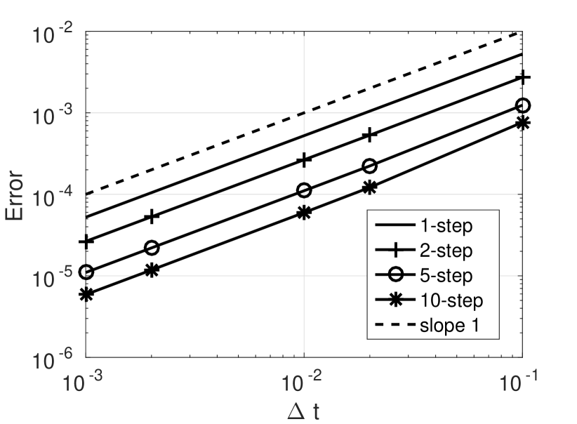
(b)

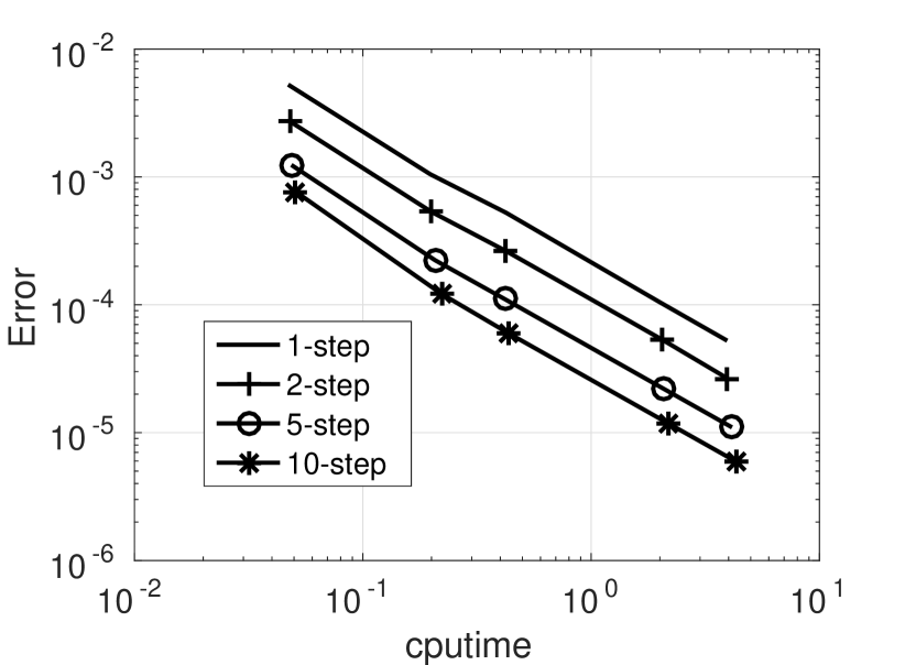
(c)

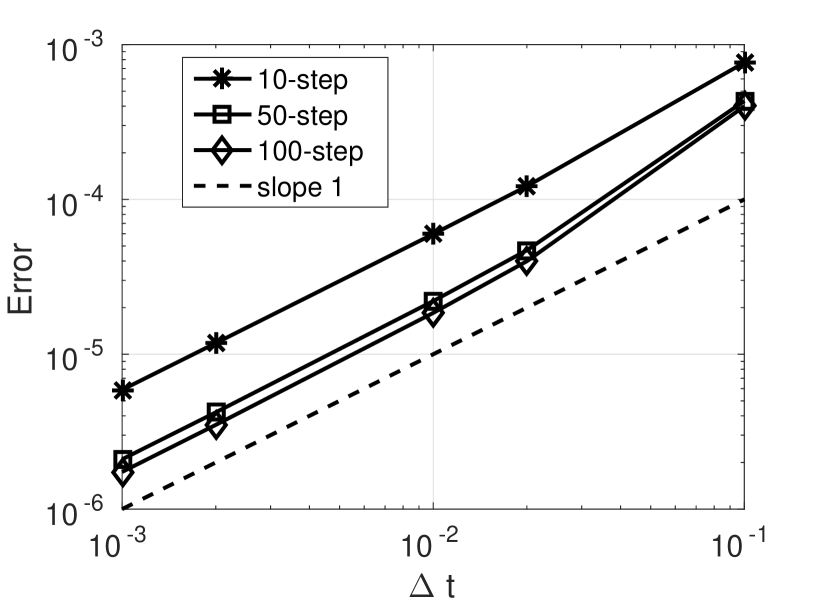
(d)

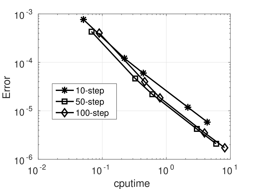
Figure 1: Results for the substepping schemes applied to the Allen-Cahn type system. a) and c) display Estimated error against timestep $\Delta t$. b) and d) display estimated error against cputime, showing efficiency.

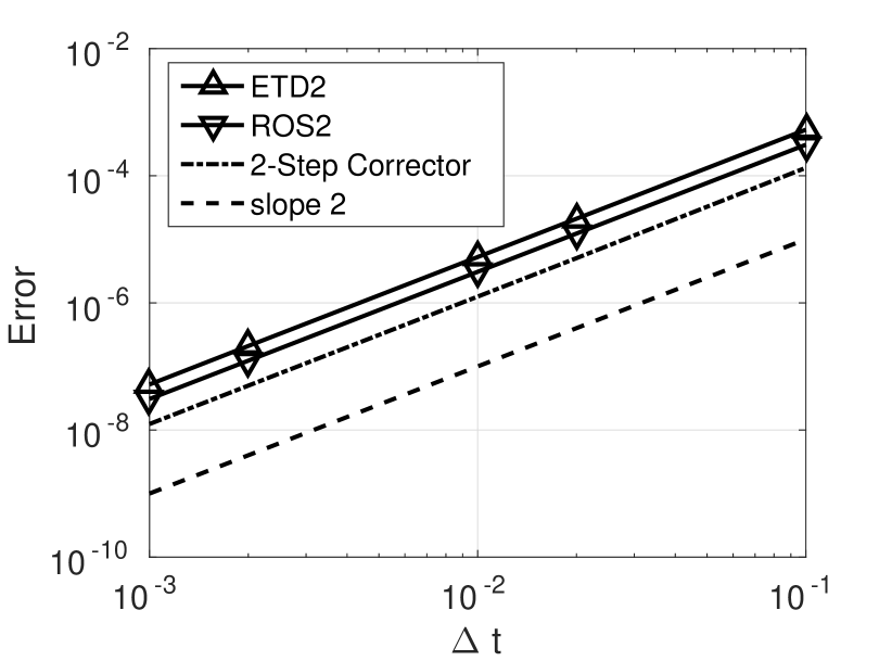
(b)

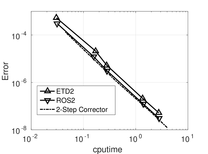
Figure 2: AC system, Comparing the second order recycling-corrector scheme with ETD2 and ROS2. a) Estimated error against timestep $\Delta t$. b) Estimated error against cputime.

In Figure 1 a) and c) we show the estimated error against $\Delta t$, for the recycling scheme with varying number of substeps $S$, ($S=1,2,5,10,50,100$). Note that $S=1$ is the standard ETD1 integtrator. The behaviour is as expected; increasing $S$ decreases the error and the scheme is first order. The diminishing returns of increasing $S$ (see (31)) can also be observed; for example compare the significant increase in accuracy in increasing $S$ from $1$ to $5$, with the lesser increase in accuracy in increasing $S$ from $5$ to $10$. Figure 1 shows this more emphatically - the increase in accuracy in increasing $S$ from $10$ to $50$ is significant, but the effect of increasing $S$ from $50$ to $100$ is very small. The limiting value of the error with respect to $S$ discussed above is clearly close to being reached here.
In Figure 1 b) and d) we plot estimated error against cputime to demonstrate the efficiency of the scheme with varying $S$. In this case increasing $S$ appears to increase efficiency until an optimal $S$ is reached, after which it decreases, as predicted. Figure 1 d) shows that the optimal $S$ lies between $50$ and $100$ for this system.
In Figure 2 we examine the 2-step corrector (48). Plot a) shows estimated error against $\Delta t$. The corrector scheme is second order as intended, and has quite high accuracy compared to the other two schemes, possibly due to the heuristic attempt to decrease the error in the leading term (see discussion in §4). In plot b) we see that the 2-step corrector is of comparable efficiency to ROS2.

In Figure 1 b) we see that for the same cputime, increasing $S$ from $1$ to $10$ decreases the estimated error by roughly an order of magnitude. We can see in Figure 1 d) that increasing $S$ from $10$ to $50$ can further decrease error for a fixed cputime, though less significantly. Comparing a fixed cputime in Figure 1 b) and Figure 2 b) indicates that the second order, 2-step corrector method can produce error more than one order of magnitude smaller than the first order recycling scheme with $S=10$.

5.2 Fracture system with Langmuir-type reaction

We approximate the solution to the PDE,

$$\frac{dv}{dt}=\nabla\cdot(\nabla Dv+Vv)-\frac{0.02}{D(\mathbf{x})^{2}}\frac{v}{1+v}.$$ (50)

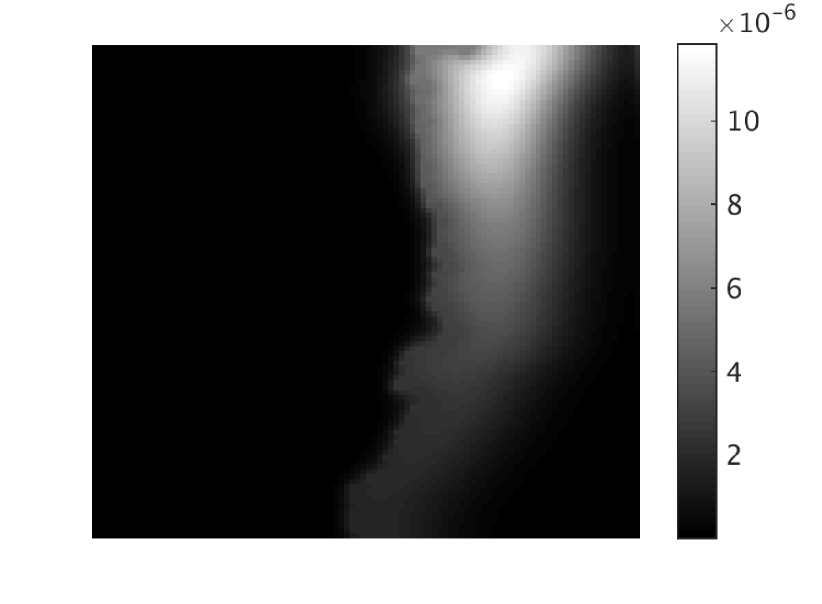
(b)

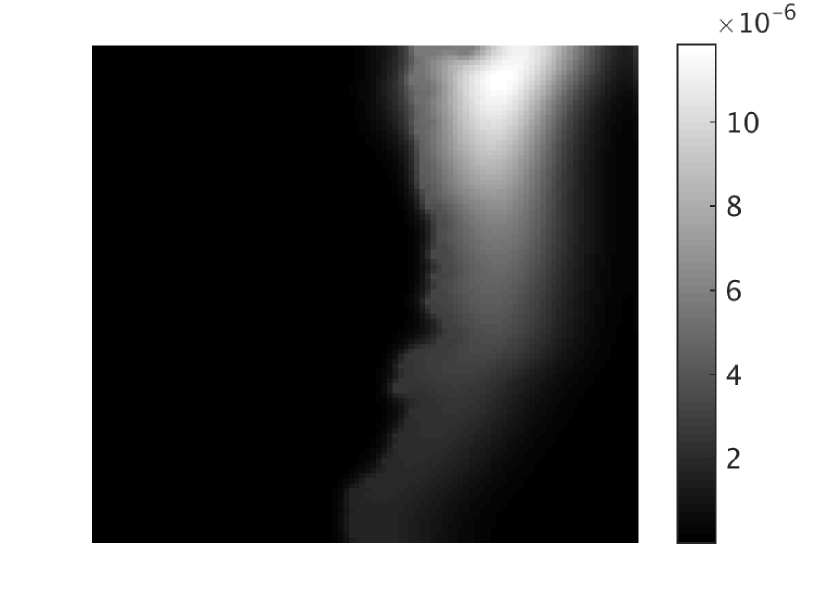
Figure 3: The final state of the fracture system with Langmuir type reaction. a) Result produced by the 2-step scheme with $\Delta t=2.4\times 10^{-4}$. b) Result produced by ETD2 with $\Delta t=2.4\times 10^{-5}$.

where $D(\mathbf{x})$ is the diffusivity and $V(\mathbf{x})$ is the velocity. In this example a single layer of cells is used, making the problem effectively two dimensional. The domain is $\Omega=10\times 10\times 10$ metres, divided into $100\times 100\times 1$ cells of equal size. We impose no-flow boundary conditions on every edge. The initial condition imposed is initial $v(\mathbf{x})=0$ everywhere except at $\mathbf{x}=(4.95,9.95)^{T}$ where $v(\mathbf{x})=1$. The diffusivity $D$ in the grid varies with $\mathbf{x}$, in a way intended to model a fracture in the medium. A subset of the cells in the 2D grid were chosen to be cells in the fracture. These cells were chosen by a weighted random walk through the grid (weighted to favour moving in the positive $y$-direction so that the fracture would bisect the domain). This process started on an initial cell which was marked as being in the fracture, then randomly chose a neighbour of the cell and repeated the process. We set the diffusivity to be $D=100$ on the fracture and $D=0.1$ elsewhere. There is also a constant velocity $V$ field in the system, uniformly one in the x-direction and zero in the other directions in the domain, i.e., $\mathbf{v}(\mathbf{x})=(1,0,0)^{T}$ , to the right in Figure 3. The initial condition was $c(\mathbf{x})=0$ everywhere except at $\mathbf{x}=(4.95,9.95)^{T}$ where $c(\mathbf{x})=1$.

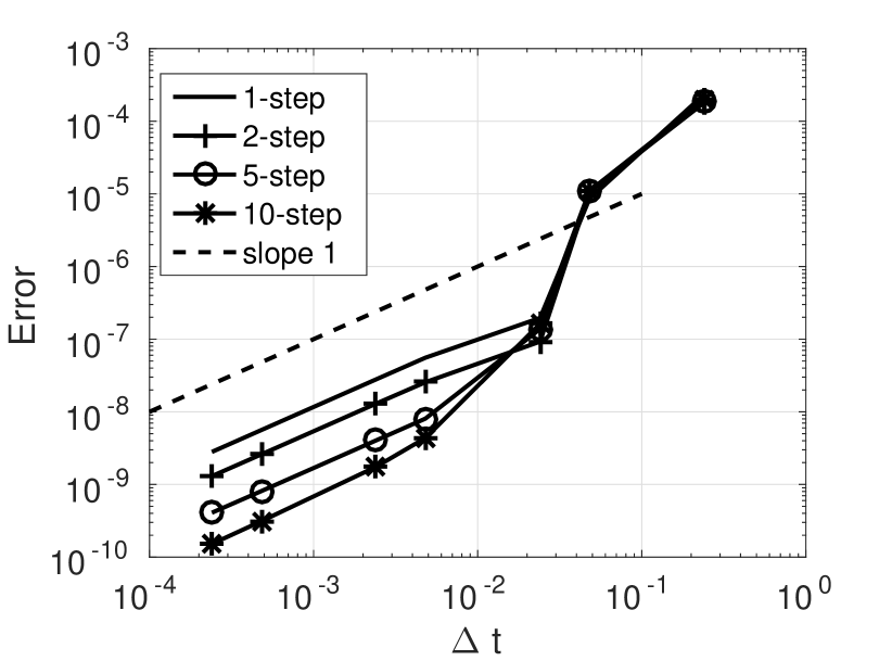
(b)

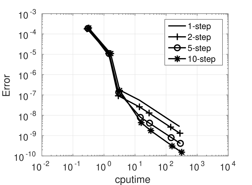
(c)

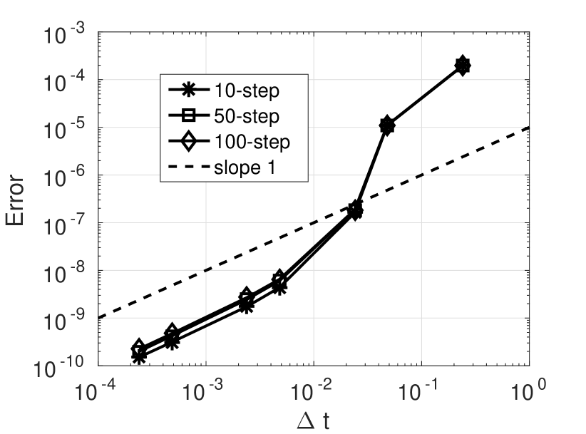
(d)

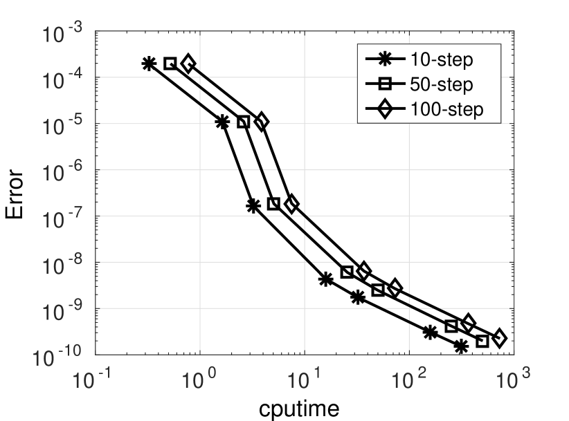
Figure 4: Results for the substepping schemes applied to the Langmuir type reaction system. a) and c) display Estimated error against timestep $\Delta t$. b) and d) display estimated error against cputime, showing efficiency. In c), points for the $50$ step scheme are marked with circles, and points with the $100$ step scheme are marked with triangles, to help distinguish the (very similar) results for the two schemes. This is also done in plot d) for consistency.

In Figure 3 we show the final state of the system at time $T=2.4$. The result in plot a) was produced with the 2-step recycling scheme with a timestep $\Delta t=2.4\times 10^{-4}$. Plot b) shows the high accuracy comparison ETD2 solve, produced with $\Delta t=2.4\times 10^{-5}$.
In Figure 4 we demonstrate the effect of increasing the number of substeps $S$ on the error. Figure 4 a) shows estimated error against timestep $\Delta t$, for schemes using $S=1,2,5,10$ substeps, while Figure 4 c) shows the same for schemes using $S=10,50,100$. Recall that $S=1$ is the standard ETD1 integtrator.

For sufficiently low $\Delta t$ we have the predicted results, with the error being first order with respect to $\Delta t$, and decreasing as $S$ increases. For $\Delta t$ too large, this is not the case. Here the Krylov subspace dimension $m$ is most likely the limiting factor as Assumption 3.1 becomes invalid. In Figure 4 b) and d) we show the efficiency by plotting the estimated error against cputime. For $\Delta t$ low enough that the substepping schemes are effective, the scheme with $10$ substeps is the most efficient.
We can see the existence of an optimal $S$ for efficiency, as predicted, in Figure 4 d), where the scheme using $S=50$ is more efficient than the scheme using $S=100$. Any increase in accuracy by increasing $S$ from $50$ to $100$ is extremely small (indeed, it is unnoticeable in Figure 4 c), and not enough to offset the increase in cputime. In fact, Figure 4 d) shows that for this experiment the scheme using $S=10$ is more efficient than both the $S=50$ and $S=100$ schemes. Figure 4 c) shows that the $S=10$ scheme is also slightly more accurate than both. This is likely because at $S=10$ the improvement in accuracy is already close to the limiting value, and greatly increasing $S$ to $50$ or $100$ only accumulates rounding errors without further benefit. Figure 4 a) shows that the improvement from $S=1$ to $S=10$ is quite significant on its own.

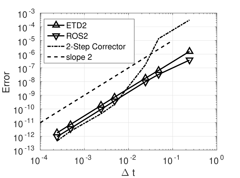
(b)

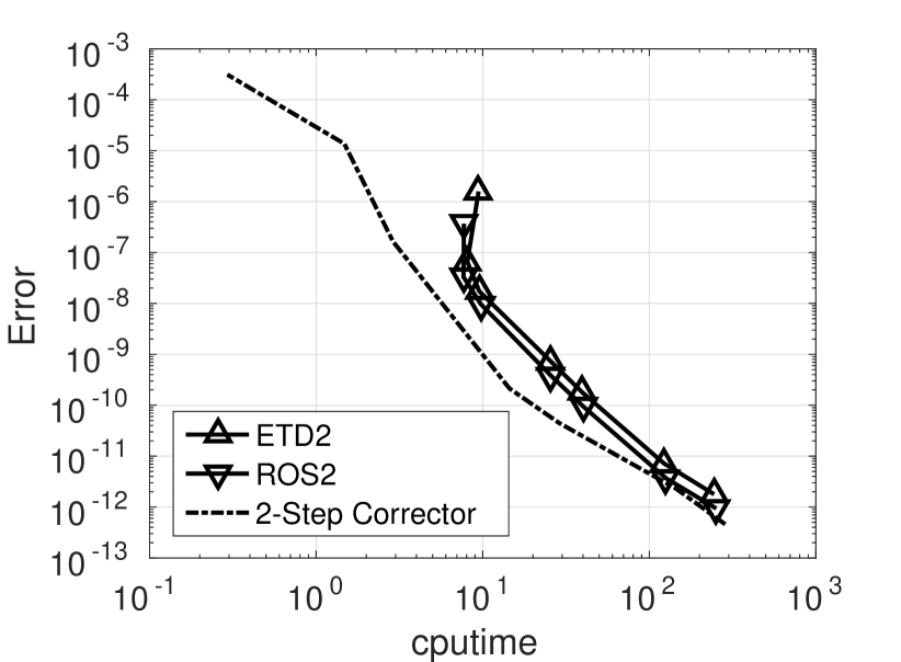
Figure 5: Langmuir type reaction system, Comparing the second order recycling-corrector scheme with ETD2 and ROS2. a) Estimated error against timestep $\Delta t$. b) Estimated error against cputime.

In Figure 5 we compare the 2-step corrector scheme against the two other second order exponential integrators, ETD2 and ROS2. Figure 5 a) shows estimated error against $\Delta t$, and we see that, like Figure 4 a), the Krylov recycling scheme does not function as intended above a certain $\Delta t$ threshold; again this is due to the timestep being too large with respect to $m$. The standard exponential integrators do not have this problem, as their timesteps are driven by phipm.m, which takes extra (non-recycled, linear) substeps to achieve a desired error. Below the $\Delta t$ threshold, the 2-step corrector scheme functions exactly as intended, exhibiting second order convergence and high accuracy. In Figure 5 b) we can observe that the 2-step corrector scheme is more efficient than the other two schemes for lower $\Delta t$, and of comparable efficiency for larger $\Delta t$.
It is interesting to compare Figure 4 a) and Figure 5 a) and note that the threshold $\Delta t$ for the corrector scheme seems to be lower than for the substepping schemes.
In Figure 4 b) we can again see that for a fixed cputime, increasing $S$ from $1$ to $10$ decreases error by roughly one order of magnitude; however Figure 4 d) shows no improvement in increasing $S$ from $10$ to $50$. Comparing Figure 4 b) and Figure 5 b) shows that the second order corrector scheme can be almost three orders of magnitude more accurate for a fixed cputime than the first order recycling scheme with $S=10$.

5.3 Large 2D Example with Random Fields

In this example the 2D grid models a domain with physical dimensions $100\times 100\times 10$; the grid is split into a $1000\times 1000\times 1$ cells. The model equation is the same as the previous example (50). The diffusivity is kept constant at $D=0.01$, while a random velocity $V$ field is used. For this we generated a random permativity field $K$, which was then used to generate a corresponding pressure field and then a velocity field in a standard way, using Darcy’s Law, see [21, 25]. The pressure $p$ field was determined by the permativity field and the Dirichlet boundary conditions $p=1$ where $y=0$ and $p=0$ where $y=100$. The initial conditions for $v$ were zero everywhere, and the boundary conditions were the same as for $p$, $v=1$ where $y=0$ and $v=0$ where $y=100$. The final time was $T=500$.

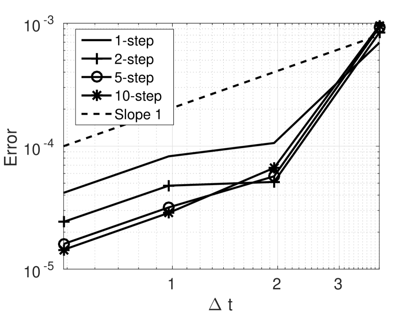
(b)

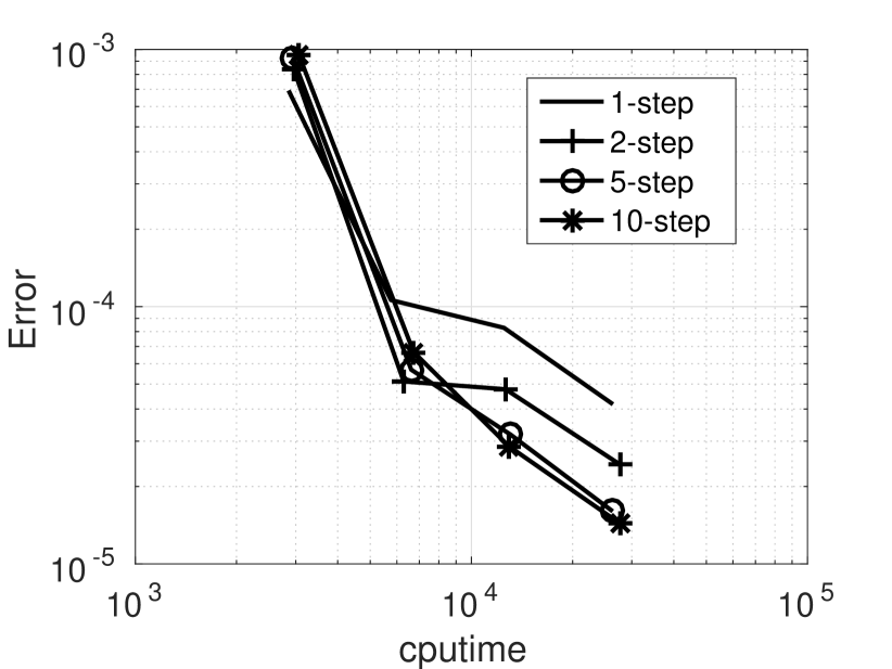
Figure 7: Results for the substepping scheme applied to the large Langmuir type reaction system in §5.3. (a) Estimated errors against timestep $\Delta t$ and (b) displays estimated error against cputime, showing efficiency. Note that for the largest timestep the error is dominated by the Krylov error as $m$ is too small for the given $\Delta t$ (c.f. Assumption 3.1 )

Due to the large size of system ($10^{6}$ unknowns) we only examine the recycling scheme and for a system of this size, it was necessary to increase $m$ to $100$ to prevent the Krylov error from being dominant. The results are shown in Figure 7. We see that, for $\Delta t$ sufficiently low, increasing $S$ decreases the error and increases the efficiency of the scheme. The improvement in efficiency between $S=5$ and $S=10$ is marginal; the optimal $S$ for this example would not be much greater than $10$.

6 Conclusions

We have extended the notion of recycling a Krylov subspace for increased accuracy in the sense of [22]. We have applied this new method to the first order ETD1 scheme and examined the effect of taking an arbitrary number $S$ of substeps. The local error has been expressed in terms of $S$, and the expression shows that the local error will decrease with $S$ down to a finite limit. The discussion in A examines construction for EEM. Results suggest that there maybe an optimal $S$ for a maximal efficiency increase and some preliminary analysis in this direction may be fuond in [21]. Convergence and existence of an optimal $S>1$ has been demonstrated with numerical experiments. Additional information from the substeps was used to form a corrector and a second order scheme. This was shown to be comparable to, or slightly better than, ETD2 and ROS2 in our tests.

The schemes currently rely on Assumption 3.1, essentially requiring that $\Delta t$ be sufficiently small and $m$ be sufficiently large, to be effective. Numerical experiments have shown how having $\Delta t$ too large can cause the schemes to become inaccurate as the error of the initial Krylov approximation becomes significant. It is already well established how the Krylov approximation error can be controlled by adapting $m$ and the use of non-recycling substeps. Applying these techniques to the schemes presented here in future work would allow them to be effective over wider $\Delta t$ ranges.

7 Acknowledgments

The authors are grateful to Prof. S. Geiger for his input into the flow simulations. The work of the Dr D. Stone was funded by the SFC/EPSRC(EP/G036136/1) as part of NAIS.

Appendix A Substepping with the scheme EEM

We now show how to apply the analysis of the substepping method to the locally third order exponential integrator scheme EEM. Applied to the system of ODEs

$$\frac{du}{dt}=g(u),$$

where $g(u)$ may not be semilinear, the scheme EEM is given by

$$u_{n+1}=u_{n}+\Delta t\phi_{1}(\Delta tJ_{n}),$$ (51)

where $J$ denotes the Jacobian of $g$ and $J_{n}=J(u_{n})$. The Jacobian $J_{n}$ is kept fixed for the entire step $\Delta t$, including recycling substeps. Therefore an $S$ step recycling scheme can be defined on EEM in exactly the same way as the recycling scheme for ETD1. Note that the Krylov subspace will be generated for $J$ and $g$ in the EEM case, i.e. $\mathcal{K}=\mathcal{K}(J_{n},g_{n})$.

With $\tilde{p}_{\tau}\equiv\tau V_{m}\varphi_{1}(\tau H_{m})V_{m}^{T}$ approximating $\tau\varphi_{1}(\tau J)$ Applying the Krylov subspace recycling scheme to EEM we have

$$u_{n+\frac{j}{S}}=u_{n}+\tilde{p}_{j\delta t}g_{n}+R_{n+\frac{j}{S}}^{S}.$$

Following the same steps as in Lemma 24 we obtain the following result.

Corollary A.1.

The remainder $R_{n+\frac{j}{S}}^{S}$ satisfies the recursion relation

$$R_{n+\frac{j+1}{S}}^{S}=\tilde{p}_{\delta t}(F_{n+\frac{j}{S}}-F_{n})+(I+\tilde{p}_{\delta t}L)R_{n+\frac{j}{S}}^{S},$$ (52)

where $F_{n+\frac{j+1}{S}}=g_{n+\frac{j+1}{S}}-J_{n}u_{n+\frac{j+1}{S}}$.

To examine the remainder term in more detail let $\hat{J}_{i}$ be the Hessian matrix

$$\hat{J}_{i}=\left(\begin{array}[]{ccc}(\hat{g}_{i})_{x_{1}x_{1}}&(\hat{g}_{i})_{x_{1}x_{2}}&\ldots\\ (\hat{g}_{i})_{x_{2}x_{1}}&(\hat{g}_{i})_{x_{2}x_{2}}&\ldots\\ \ldots&\ldots&\ldots\end{array}\right),$$

where $\hat{g}_{i}$ is the $i$th entry of the vector $g$. Let the tensor $\hat{\mathbf{J}}$ be a vector with the matrix $\hat{J}_{i}$ in its $i$th entry. We can now Taylor expand the remainder $R_{n+\frac{j}{S}}^{S}$ from (52) to find the local error of the EEM scheme with recycled substeps.

Lemma A.2.

For the EEM recycling scheme, the leading term of $R_{n+\frac{j}{S}}^{S}$ satisfies

$$R_{n+\frac{j}{S}}^{S}=\alpha(j)\delta t^{3}V_{m}V_{m}^{T}g_{n}^{T}\hat{\mathbf{J}}g_{n}+O(\delta t^{4})$$

where $\alpha(j)=(2j^{3}-3j^{2}+j)/24$.

Proof.

By induction. The base case is true for $j=1$ with $\alpha(1)=0$ since there is no recycling at that step. Assume true for some $j$. Consider $g_{n+\frac{j}{S}}$,

$$g_{n+\frac{j}{S}}=g(u_{n+\frac{j}{S}})=g(u(t)+j\delta tg(t)+\frac{1}{2}(j\delta t)^{2}Jg+O(\delta t^{3})),$$

to second order this is

$$g_{n+\frac{j}{S}}=g_{n}+J\left(j\delta tg_{n}+\frac{1}{2}(j\delta t)^{2}Jg_{n}\right)+\frac{(j\delta t)^{2}}{2}g_{n}^{T}\hat{\mathbf{J}}g_{n}+O(\delta t^{3}),$$

where we have made use of the local error assumption $u(t_{n})=u_{n}$. Then,

$$F_{n+\frac{j}{S}}-F_{n}=g_{n+\frac{j}{S}}-g_{n}-Ju_{n+\frac{j}{S}}+Ju_{n}$$

and since $u_{n+\frac{j}{S}}=u_{n}j\delta tg_{n}+\frac{(j\delta t)^{2}}{2}Jg_{n}+O(\delta t^{3})$ up to second order and the induction hypothesis we have

$$F_{n+\frac{j}{S}}-F_{n}=\frac{(j\delta t)^{2}}{2}g_{n}^{T}\hat{\mathbf{J}}g_{n}+O(\delta t^{3}).$$

Now consider

$$\tilde{p}_{\delta t}\left(F_{n+\frac{j}{S}}-F_{n}\right)=\frac{j^{2}(\delta t)^{3}}{2}V_{m}V_{m}^{T}g_{n}^{T}\hat{\mathbf{J}}g_{n}+O(\delta t^{4})$$

The induction relation for $R_{n+\frac{j+1}{S}}^{S}$ then gives us

$$R_{n+\frac{j+1}{S}}^{S}=\frac{j^{2}(\delta t)^{3}}{2}V_{m}V_{m}^{T}g_{n}^{T}\hat{\mathbf{J}}g_{n}+(I+\tilde{p}_{\delta t}J)R_{n+\frac{j}{S}}^{S}+O(\delta t^{4})$$

which to leading order this is

$$R_{n+\frac{j+1}{S}}^{S}=\left(\frac{j^{2}}{2}+\alpha(j)\right)\delta t^{3}V_{m}V_{m}^{T}g_{n}^{T}\hat{\mathbf{J}}g_{n}+O(\delta t^{4}).$$

So $\alpha(j+1)=\frac{j^{2}}{2}+\alpha(j)$, $\alpha(1)=0.$ which is satisfied by the given $\alpha(j)$. ∎

We now combine the leading term of the remainder $R$ and the known local error of EEM

$$\frac{1}{6}\Delta t^{3}g^{T}\hat{\mathbf{J}}g.$$

(see, for example, [21]) to find the local error of the new recycling scheme.

Corollary A.3.

The leading term of the local error of the $S$ step recycling scheme for EEM at the end of a timestep is

$$\frac{\Delta t^{3}}{6}\left(I-\left(\frac{2S^{2}-3S+1}{2S^{2}}\right)V_{m}V_{m}^{T}\right)g^{T}\hat{\mathbf{J}}g.$$

From this we can predict similar properties to the ETD1 recycling scheme. This extends the work of [22], where the recycling substepping EEM scheme was used for a single substep.

(a)

(a)

(a)

(a)

(a)

(a)

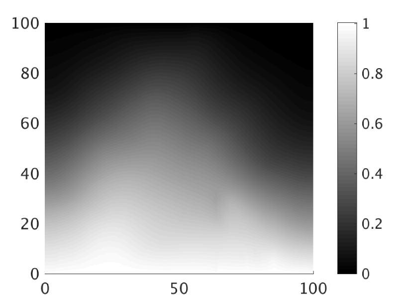
(b)

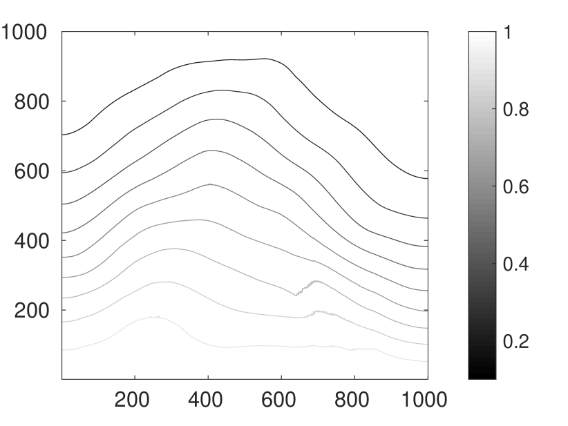
Figure 6: Result for the example in §5.3, in which solute enters through the lower boundary and flows according to a random velocity field. Produced by the 10-step recycling scheme with $\Delta t=0.2441$, i.e. $2048$ steps. a) Shows the system at the final time $T=500$; the axes indicates the physical dimensions (i.e., the domain is $100\times 100$ metres). b) Is a corresponding contour plot for clarity; the axes indicate the cells in the finite volume grid (i.e., the grid has $1000$ cells along each side).

(a)

References

- [1] S. M. Cox and P. C. Matthews. Exponential time differencing for stiff systems. Journal of Computational Physics, 176:430–455, 2002.
- [2] M. Caliari, M. Vianello, and L. Bergamaschi. The LEM exponential integrator for advection-diffusion-reaction equations. J. Comput. Appl. Math., 210(1-2):56–63, 2007.
- [3] M. Hochbruck, Alexander O., and J. Schweitzer. Exponential Rosenbrock-type methods. SIAM J. Numer. Anal., 47(1):786–803, 2008/09.
- [4] M. Caliari and A. Ostermann. Implementation of exponential Rosenbrock-type integrators. Appl. Numer. Math., 59(3-4):568–581, 2009.
- [5] M. Hochbruck and A Osterman. Exponential integrators. Acta Numerica, pages 209–286, 2010.
- [6] B. Minchev and W. Wright. A review of exponential integrators for first order semilinear problems.
- [7] A. K. Kassam and L. N. Trefethen. Fourth-order time-stepping for stiff PDEs. SIAM J. Sci. Comput., 26(4):1214–1233 (electronic), 2005.
- [8] C. Moler and C. Van Loan. Nineteen dubious ways to compute the exponential of a matrix. SIAM Rev., 20(4):801–836, 1978.
- [9] A. H. Al-Mohy and N. J. Higham. Computing the action of the matrix exponential, with an application to exponential integrators. SIAM J. Sci. Comput., 33(2):488–511, 2011.
- [10] I. Moret and P. Novati. An interpolatory approximation of the matrix exponential based on Faber polynomials. J. Comput. Appl. Math., 131(1-2):361–380, 2001.
- [11] J. Baglama, D. Calvetti, and L. Reichel. Fast Leja points. Electron. Trans. Numer. Anal., 7:124–140, 1998. Large scale eigenvalue problems (Argonne, IL, 1997).
- [12] L. Bergamaschi, M. Caliari, and M. Vianello. The ReLPM exponential integrator for FE discretizations of advection-diffusion equations. In Computational science—ICCS 2004. Part IV, volume 3039 of Lecture Notes in Comput. Sci., pages 434–442. Springer, Berlin, 2004.
- [13] A. Martínez, L. Bergamaschi, M. Caliari, and M. Vianello. A massively parallel exponential integrator for advection-diffusion models. J. Comput. Appl. Math., 231(1):82–91, 2009.
- [14] L. Bergamaschi, M. Caliari, A. Martinez, and M. Vianello. Comparing Leja and Krylov approximations of large scale matrix exponentials. In Computational Science–ICCS 2006, pages 685–692. Springer, 2006.
- [15] M. Caliari, M. Vianello, and L. Bergamaschi. Interpolating discrete advection-diffusion propagators at Leja sequences. J. Comput. Appl. Math., 172(1):79–99, 2004.
- [16] Y. Saad. Analysis of some Krylov subspace approximations to the matrix exponential operator. SIAM J. Numer. Anal., 29(1):209–228, 1992.
- [17] M. Hochbruck and C. Lubich. On Krylov subspace approximations to the matrix exponential operator. SIAM J. Numer. Anal., 34(5):1911–1925, 1997.
- [18] R. B. Sidje. Expokit: a software package for computing matrix exponentials. ACM Transactions on Mathematical Software (TOMS), 24(1):130–156, 1998.
- [19] J. Niesen and W. Wright. A Krylov subspace algorithm for evaluating the -functions in exponential integrators. arXiv:0907.4631v1, 2009.
- [20] M. Tokman and J. Loffeld. Efficient design of exponential-Krylov integrators for large scale computing. Procedia Computer Science, 1(1):229–237, 2010.
- [21] D. Stone. Asynchronous and exponential based numerical schemes for porous media flow. PhD thesis, Heriot-Watt, 2015.
- [22] E. Carr, T. Moroney, and I. Turner. Efficient simulation of unsaturated flow using exponential time integration. Applied Mathematics and Computation, 217:6587–6596, 2011.
- [23] M. Hochbruck and A. Ostermann. Explicit exponential Runge-Kutta methods for semilinear parabolic problems. SIAM J. Numer. Anal., 43(3):1069–1090 (electronic), 2006.
- [24] Y Saad. Iterative Methods for Sparse Linear Systems. ITP, 1996.
- [25] K. A. Lie, S. Krogstad, I. S. Ligaarden, H. M. Natvig, J. R.and Nilsen, and B. Skaflestad. Open-source matlab implementation of consistent discretisations on complex grids. Computational Geosciences, 16(2):297–322, 2012.