Slipping Magnetic Reconnection of Flux Rope Structures as a Precursor to an Eruptive X-class Solar Flare

Abstract

We present the quasi-periodic slipping motion of flux rope structures prior to the onset of an eruptive X-class flare on 2015 March 11, obtained by the Interface Region Imaging Spectrograph (IRIS) and the Solar Dynamics Observatory (SDO). The slipping motion occurred at the north part of the flux rope and seemed to successively peel off the flux rope. The speed of the slippage was 30$-$40 km s^-1, with an average period of 130$\pm$30 s. The Si iv 1402.77 Å line showed a redshift of 10$-$30 km s^-1 and a line width of 50$-$120 km s^-1 at the west legs of slipping structures, indicative of reconnection downflow. The slipping motion lasted about 40 min and the flux rope started to rise up slowly at the late stage of the slippage. Then an X2.1 flare was initiated and the flux rope was impulsively accelerated. One of the flare ribbons swept across a negative-polarity sunspot and the penumbral segments of the sunspot decayed rapidly after the flare. We studied the magnetic topology at the flaring region and the results showed the existence of a twisted flux rope, together with quasi-separatrix layers (QSLs) structures binding the flux rope. Our observations imply that quasi-periodic slipping magnetic reconnection occurs along the flux-rope-related QSLs in the preflare stage, which drives the later eruption of the flux rope and the associated flare.

1 Introduction

Solar flares, often associated with filament eruptions and coronal mass ejections (CMEs), are major drivers of space weather (Gosling et al. 1991). During these events, magnetic free energy is converted to radiation, energetic particle acceleration and kinetic energy of plasma through magnetic reconnection (Forbes et al. 2006). The two-dimensional (2D) standard flare model (Shibata & Magara 2011) was applied to explain many flare phenomena. In this model, magnetic reconnection takes place at the magnetic null-point under the eruptive flux rope and flare ribbons, cusp-shaped loops and post-flare loops are thus formed (Schmieder et al. 1996; Milligan & Dennis 2009). Nevertheless, actual flares are intrinsically three-dimensional (3D) events (Janvier et al. 2015). The 2D standard flare model may not explain some features of flares (Wang & Liu 2012), such as the morphology of the ribbons and the motions of small-scale bright knots along ribbons. Therefore, a comprehensive understanding of the 3D physical processes of flares is important, particularly magnetic reconnection.

By analyzing the magnetic topology and geometry of the flaring region, the locations where magnetic reconnection could occur can be well understood. In 2D, magnetic reconnection is initially considered to occur at a null point (Sweet 1958), where the magnetic field vanishes. A separatrix surface is another topological feature preferential for forming the strong electric current sheets, through which the field line connectivity is discontinuous (Longcope 2005). Gorbachev & Somov (1988) first found the correspondence of the separatrices obtained from the potential magnetic field model and flare ribbons. Afterwards, several studies found the relationship between the observed flare ribbons and the computed separatrices from potential and linear force-free field models (Demoulin et al. 1993; van Driel-Gesztelyi et al. 1994; Mandrini et al. 1995, 2014). However, the flares without null points and the associated separatrices are observed (Demoulin et al. 1994). Therefore, Priest & Démoulin (1995) and Demoulin et al. (1996) introduced the concept of quasi-separatrix layers (QSLs), where the magnetic connectivity shows strong gradients, but is still continuous. The magnetic field distortion is defined by a strong value of the squashing degree Q (Titov et al. 2002; Titov 2007). QSLs are preferential locations for magnetic reconnection because high electric current density regions can be formed at QSLs during the magnetic field evolution (Aulanier et al. 2005; Wilmot-Smith et al. 2009). Savcheva et al. (2012, 2015) found the close correspondence between flare ribbons and the locations of QSLs obtained from the data-constrained nonlinear force-free field (NLFFF) models created with the flux rope insertion method.

When magnetic reconnection occurs in the QSLs, the field lines crossing the QSLs exchange their connectivity with the neighboring fields and their motion is seen as an apparent slipping motion of field lines (Priest & Démoulin 1995; Demoulin et al. 1996; Aulanier et al. 2006, 2007; Masson et al. 2009). Priest & Démoulin (1995) analytically predicted that the magnetic reconnection in the QSLs is characterized by the flipping of magnetic field lines as they slip rapidly through the plasma. If the speed of the apparent motion of the field lines is at super-Alfvénic time scales, the process is the so-called “slip-running reconnection.” While if the change of connectivity is sub-Alfvénic, this is said to be “slipping reconnection” (Aulanier et al. 2006). In the 3D magnetohydrodynamic (MHD) simulation of Janvier et al. (2013), the slipping motion speed is not constant as time goes by and it could be sub- or super-Alfvénic. The simulation of Janvier et al. (2013) generally matches the recent observations of Li & Zhang (2014), who presented the slippage of flux rope structures along a hook-shaped flare ribbon. The slipping motion delineated a “triangle-shaped flag surface”, implying one-half of the QSL structure. Observational studies showed the slipping motion of individual flare loops and small-scale bright knots in flare ribbons during eruptive flares (Dudík et al. 2014, 2016; Zheng et al. 2016; Sobotka et al. 2016), which satisfies the slipping reconnection regime. Based on the observations from the Solar Dynamics Observatory (SDO; Pesnell et al. 2012) and the Interface Region Imaging Spectrograph (IRIS; De Pontieu et al. 2014), Li & Zhang (2015) found that the flare loops and flare ribbon substructures both exhibited the quasi-periodic slipping motion with a period of about 3-6 min.

The direct observations about the slipping nature of 3D magnetic reconnection are very rare due to the low spatial resolution and limited channels of previous instruments. Recently, the rich high-quality observations provide us a chance to study the 3D evolution process of flares. In this paper, we report that the flux rope structures exhibited the quasi-periodic slippage along the flux-rope-related QSLs in the preflare stage, which drives the initiation of an X2.1 flare on 2015 March 11 and the later eruption of the flux rope. The previous studies reported the slipping motions of flare loops and flux rope structures during the flare process, however, the preflare slipping motion of flux rope structures has never been reported before. The outline of the paper is as follows: the observations and data analysis are presented in Section 2, Section 3 presents the results of preflare activities and the later eruption, Section 4 shows the summary and discussion.

2 Observations and Data Analysis

We combine data from the SDO and the IRIS to investigate the preflare slipping motion of flux rope structures and the later eruption process. Full sun images from the Atmospheric Imaging Assembly (AIA; Lemen et al. 2012) are available with a resolution of $\sim$0$\arcsec$.6 per pixel and a cadence of 12 seconds for the EUV passbands. The observations of AIA 1600 Å, 304 Å and 131 Å passbands are used. The full-disk line-of-sight (LOS) magnetograms and the photospheric vector magnetic field data of the AR observed by the Helioseismic and Magnetic Imager (HMI; Scherrer et al. 2012) are also applied. The IRIS 1330 Å, 1400 Å and 2832 Å slit-jaw images (SJIs) cover the majority of the active region (AR), with a spatial sampling of $\sim$0$\arcsec$.33 per pixel and a cadence of about 20 seconds for each passband. The spectral data are taken in a 4-step raster mode with steps of 2$\arcsec$, giving a total field of view (FOV) of 6$\arcsec$$\times$ 119$\arcsec$. Each raster step takes about 5 s (2 s exposure) and the spectral sampling is $\sim$0.025 Å pixel^-1. We analyze the spectroscopic observations of the Si iv 1402.77 Å line formed in the transition region with a temperature of $\sim$ 80000 K (Tian et al. 2014) and apply a single-Gaussian fit to obtain the Doppler shift and line width at the locations of the slipping structures (Peter et al. 2014).

3 Results

3.1 Overview of Productive AR 12297

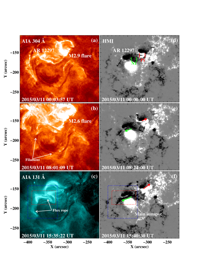
Figure 1: Time sequence of AIA 304 Å images, 131 Å image and HMI LOS magnetograms showing the evolving AR 12297 on 2015 March 11. Positive patch P1 and negative patch N1 in panel (d) are an emerging bipolar pair in the AR center. Red and green arrows respectively denote the shearing motions of the emerging flux P1 and N1. The red rectangles in panels (c) and (f) show the FOV of Figures 2$-$3, 5(a) and 5(d). The blue rectangles show the FOV of Figure 7.

The target flare of this study occurred in NOAA AR 12297 in the southern hemisphere on 2015 March 11. This AR produced many flares including one X- and 18 M-class events since its appearance at the east limb on March 07. Before the occurrence of the X2.1 flare, two M-class flares (M2.9 and M2.6 in Figures 1(a)-(b)) occurred at around 00:00 and 08:00 UT on March 11. The region also produced several C-Class flares during 5 hours before the X-class flare. The small flares may reduce the constraint of the flux rope system by the rearrangement of magnetic fields, which makes it easier for the later eruption of the flux rope and the X-class flare. A bipolar pair (P1$-$N1) emerged in the AR center and the emerging opposite-polarity magnetic flux gradually separated from each other (Figures 1(d)-(f)). Simultaneously, strong shearing motions were observed with positive patch P1 continuously moving to the northwest (red arrows) and negative patch N1 drifting to the southeast (green arrows). A hook-shaped filament (length of $\sim$150 Mm) was located at the AR (Figure 1(b)), and at the east part of the filament, a flux rope could be observed in 131 Å channel (Figure 1(c)). The north end of the flux rope anchored in the main sunspot with positive-polarity magnetic fields (Figure 1(f)).

3.2 Slipping Motion of Flux Rope Structures

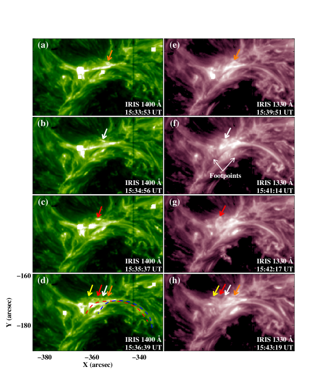
Figure 2: Slipping motion of flux rope structures viewed in IRIS 1400 Å and 1330 Å images (see Animation 1400-slippage). The orange, white, red and yellow arrows in panels (a)-(d) trace the apparent slipping motion of flux rope structures from the west to the east. The west three arrows in panel (d) are the duplicates of the arrows in panels (a)-(c). The arrows in panels (e)-(h) represent another process of the slippage from the west to the east and the meanings are the same as the left column. Red and blue dashed curves in panel (d) outline two flux rope structures.

At the north part of the flux rope, the 1400 Å and 1330 Å SJIs showed multiple bright loop structures (Figure 2; see Animation 1400-slippage). These loop structures (dashed curves in Figure 2(d)) were highly sheared around the main sunspot. Starting from about 15:27 UT, the bright structures successively slipped toward the east and seemed to peel off the flux rope. Two of the slipping processes from the west to the east were respectively shown in Figures 2(a)-(d) and 2(e)-(h). It is not the same “clump” of brightness (pointed by arrows) observed at each time, but new flux rope structures. The slipping motion was evident at the loop tops and the eastern footpoints. The eastern footpoints of the loops are relatively scattered in the east-west direction (Figure 2(f)). While the western part of the loops is concentrated and the slippage could not be clearly observed. Note that the term “slipped” or “slipping” is only the phenomenological term.

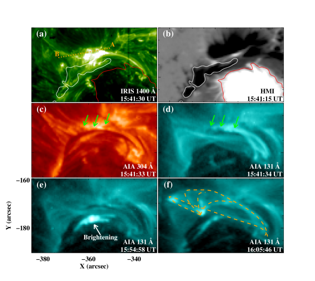
Figure 3: Multi-wavelength observations and LOS magnetogram from the IRIS and SDO. The red and white contours in panels (a)-(b) are the magnetic fields at $\pm$ 500 G levels at the ends of slipping structures. Dotted line “A$-$B” (panel (a)) shows the cut position used to obtain the time-distance plots shown in Figures 4(a)-(c). Green arrows in panels (c)-(d) point to the slipping dark structures viewed in 304 Å and 131 Å images. The dashed curves in panel (f) delineate a fan-shaped surface at the late stage of slipping motion.

The comparison of HMI magnetograms and 1400 Å images shows that the west footpoints of the slipping structures are located at positive-polarity magnetic fields of the main sunspot and the east footpoints are at negative-polarity magnetic fields (Figures 3(a)-(b)). The slipping structures seem obscure in 304 Å and 131 Å images (Figures 3(c)-(d)), probably because of the low spatial resolution of AIA EUV data and the blocking effect of filament materials along the LOS direction. In IRIS 1400 Å observations, the slipping structures appear as bright structures (Figure 3(a)). However, in AIA EUV images, both the dark and bright slipping structures are observed (arrows in Figures 3(c)-(d)). We suggest that the dark structures in 304 Å and 131 Å images correspond to filament materials, which are not evident in the optically thin lines such as 1400 Å and 1330 Å formed at transition region temperatures (Li & Zhang 2016). At about 15:53 UT, EUV brightenings were observed at the east footpoints of slipping structures (Figure 3(e)). Then the brightenings extended towards the southeast and lasted about 4 minutes. At the late stage of the slipping motion, a fan-shaped surface (delineated by dashed curves in Figure 3(f)) appeared overlying the filament in the 131 Å channel.

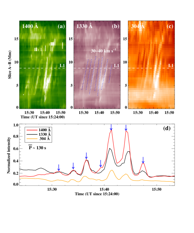
Figure 4: Panels (a)-(c): time-distance plots along slice “A$-$B” (dotted line in Figure 3(a)) at 1400 Å, 1330 Å and 304 Å showing the quasi-periodic slippage of flux rope structures. Panel (d): horizontal slices along the dashed lines (“L1”) in panels (a)-(c). $\overline{P}$ represents the average period ($\sim$ 130 s), and blue arrows point to the peaks of intensity at 1400 Å.

For investigating the kinematic evolution of the slipping structures, the time-distance plots obtained along the cut“A$-$B” (Figure 3(a)) are shown in Figure 4. Several moving intensity features are displayed in the time-distance plots of 1400 Å and 1330 Å (Figures 4(a)-(b)), and each strip denotes the apparent slipping motion of flux rope structures. The 304 Å time-distance plot shows alternately bright and dark strips (Figure 4(c)). The slippage of flux rope structures is almost at a constant velocity of 30$-$40 km s^-1 and the propagating distance is about 10 Mm. The appearance of flux rope structures and the slipping motion are intermittent and quasi-periodic. Between 15:27 UT and 15:48 UT, about seven bright strips were observed. The 1400 Å and 1330 Å profiles along “L1” (Figures 4(a)-(c)) are approximately consistent (Figure 4(d)). The time intervals between two neighboring peaks range from 102 s to 153 s, and the average period is about 130 s. The small peak just before 15:40 UT in 1400 Å profile was also selected for calculating the period of the slipping motion. As shown in Figures 4(a)-(b), there is indeed a weak and thin strip at this time. There is no clear signature in 1400 Å profile probably because the smoothing process of horizontal slices along the “L1” weakens the signal. Moreover, the peak before 15:30 UT in 1330 Å was not included while analyzing the quasi-periodic pattern. As seen from the 1330 Å stack plot (Figure 4(b)), this peak corresponds to the stationary brightening, which is not related to the slipping structure. The intensity variation in the 304 Å profile is smaller than 1400 Å and 1330 Å profiles, and about five peaks could be clearly discerned in the 304 Å profile.

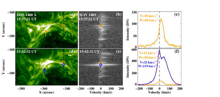
Figure 5: Left column: IRIS 1400 Å images displaying the slipping flux rope structures. The orange and blue diamonds denote the intersections of the loop-like structures and the slit. The arrows point to the brightenings at the east footpoints of analyzed structures. Middle column: simultaneous appearance of the Si iv 1402.77 Å spectra in the slit range of panels (a) and (d). Right column: profiles of the Si iv line at the selected locations. The orange dotted curves are the single-Gaussian fitting profiles. The red dotted curve is the double-Gaussian fitting profile.

The spectroscopic properties at the western legs of slipping structures are investigated and displayed in Figure 5. At 15:37:21 UT, the brightenings at the east end of a loop-like structure were observed (orange arrow in Figure 5(a)). The intersection of the loop structure and the IRIS slit was at the west leg of the analyzed structure (orange diamonds in Figures 5(a)-(b)). Applying the single Gaussian fitting of Si iv 1402.77 Å line, we get a redshift of $\sim$ 18 km s^-1 at the western leg of the slipping structure, with the line width of about 50 km s^-1 (Figure 5(c)). The background location used to correct the center is not displayed, for it is beyond the FOV of Figure 5. Then the loop structures continually slipped to the east. At about 15:42:32 UT, the intersections of two loop structures and the IRIS slit were selected (orange and blue diamonds in Figures 5(d)-(e)). Meanwhile, the brightenings appeared at the east end of one loop structure (blue arrow in Figure 5(d)). Similarly, the profiles of the Si iv line at west legs of the two structures are fitted and both exhibit evident redshifts (Figures 5(e)-(f)). For the north location (orange diamonds in Figures 5(d)-(e)), the redshift velocity is about 12 km s^-1 and the line width is $\sim$ 58 km s^-1 (orange curves in Figure 5(f)). The Si iv profile at the west leg of the south brighter structure shows two peaks, with one peak at the line center and the other at the red wing (blue solid curve in Figure 5(f)). The line-profile at this location was fitted by a double-Gaussian function. The first peak comes from the background emission and the second peak is from the west leg of the slipping structure. The slipping reconnection at the east part causes the outflow along the loop structure and thus the line profile at the west leg is redshifted. The double Gaussian fitting shows a larger redshift of about 32 km s^-1 at the south brighter structure, with the line width reaching about 119 km s^-1 (red dotted curve in Figure 5(f)). The uncertainty of the redshifts is $\sim$ 1 km s^-1 and that of the widths is about 2 km s^-1. They are estimated according to the 1-sigma error in GAUSSFIT function.

3.3 Magnetic Topology Around the Main Sunspot

We obtain the 3D coronal magnetic field by the NLFFF extrapolation method (Wheatland et al. 2000; Wiegelmann 2004). The vector magnetogram for the extrapolation is at 16:04 UT before the flare from the Space-weather HMI Active Region Patches, in which the 180° ambiguity and the projection effect have already been resolved (Sun et al. 2013; Bobra et al. 2014). Before the extrapolation, the vector magnetogram data have undergone an additional preprocessing to remove the net force and torque (Wiegelmann et al. 2006). Moreover, based on the extrapolated results, we calculated the 3D squashing factor, $Q$, with the method proposed by Pariat & Démoulin (2012). The $Q$ factor is a measurement of the gradient of the magnetic field connectivity, which is usually used to determine the QSL (Titov et al. 2002).

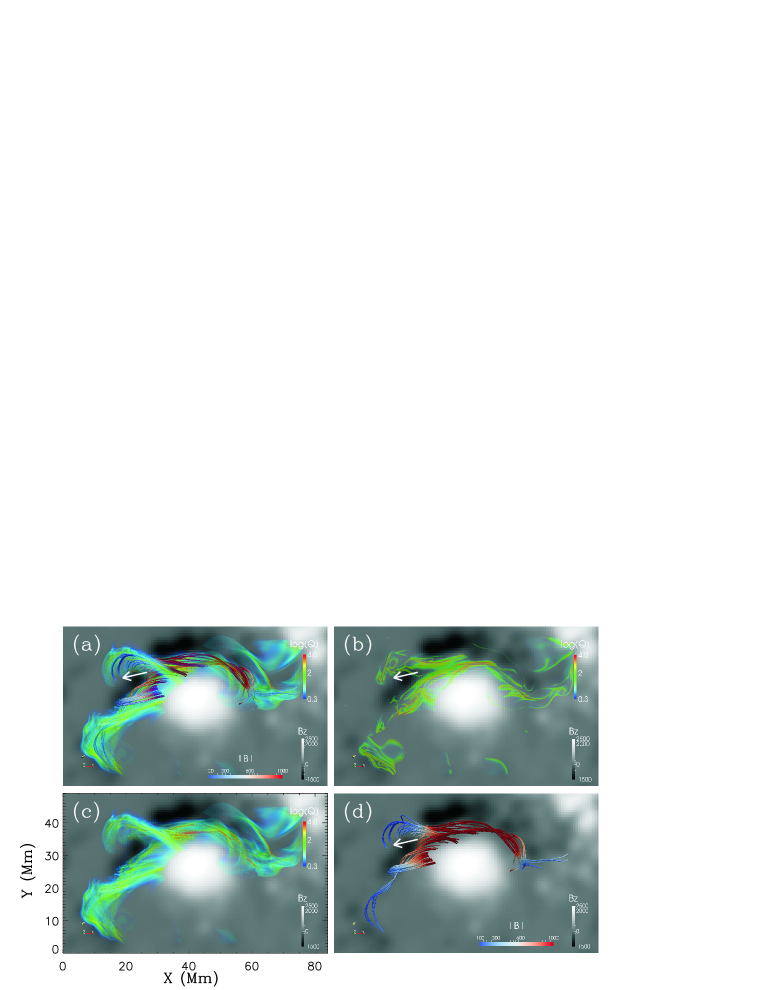
Figure 6: Topology of the extrapolated magnetic field. Panels (a), (c), and (d): field lines of the flux rope and its associated 3D QSL. Panel (b): The intersection of the QSL with the bottom boundary. The background shows the photospheric vertical magnetic field at 16:04 UT. White arrows represent the slipping motion of flux rope structures before the flare.

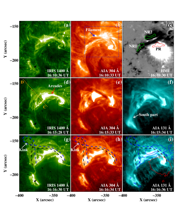
Figure 7: Eruption of the flux rope observed by the IRIS and SDO (see Animations 1400-eruption and 131-eruption). The blue rectangle in panel (b) denotes the FOV of Figures 9(a)-(f). The red and green curves in panel (c) are the contours of brightenings in the 1600 Å image at the flare peak time, displaying one positive (PR) and two negative flare ribbons (NR1 and NR2). Dotted line “C$-$D” (panel (d)) shows the cut position used to obtain the time-distance plots shown in Figure 8. Blue and black curves in panels (g)-(i) outline partial structures of the flux rope. The red and blue contours in panel (i) are the magnetic fields at $\pm$ 450 G levels.

The extrapolation results show the existence of a twisted flux rope around the main sunspot before the eruption (Figure 6), similar to the SDO and the IRIS observations. We only show the extrapolation results at 16:04 UT prior to the largest flare as we are focusing on the magnetic topology during the period of preflare motion. The western footpoints of the flux rope are located at the positive-polarity sunspot and the eastern ones are at a small negative-polarity sunspot and facula region. The 3D QSL structures are surrounding the flux rope. The intersection of the QSLs with the lower boundary approximately overlaps the locations of flare ribbons (Figures 6(b) and 7(c)). The correspondence of the intersection of the QSL with bottom boundary and flare ribbons has been reported before (Yang et al. 2015; Savcheva et al. 2015; Zhao et al. 2016). The comparison of the extrapolated magnetic field and the observations (Figures 2-3) shows that the magnetic field lines with negative-polarity footpoints along the east-west direction probably correspond to the slipping structures (white arrows in Figure 6). As seen in Figures 3(a)-(b), the east ends of slipping structures are located at the negative-polarity magnetic fields and extend along the east-west direction. The magnetic field lines at the north of white arrows in Figure 6 show a similar feature. While the field lines cross the overlying QSL, they undergo a succession of reconnection processes and result in the apparent slipping motion towards the east.

3.4 Flux Rope Eruption and Associated X2.1 Flare

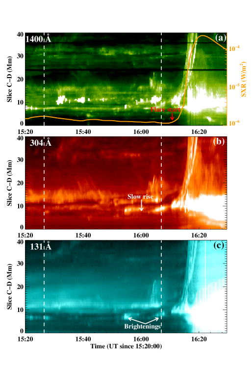
Figure 8: Time-distance plots along slice “C$-$D” (dotted line in Figure 7(d)) at 1400 Å, 304 Å and 131 Å showing the kinematic evolution of the erupting flux rope. The orange curve in panel (a) shows GOES SXR 1-8 Å flux of the associated X2.1 flare. Two dashed lines in each panel denote the time interval between 15:27 UT and 16:07 UT when the slipping motion of flux rope structures occurred.

The slipping motion of flux rope structures lasted about 40 min from 15:27 UT to 16:07 UT. At the late stage of the slippage, the entire flux rope became unstable and started to erupt from about 16:00 UT. Figure 7 shows the multi-wavelength appearance of the eruptive event and the corresponding magnetogram observed by the IRIS and the SDO (see Animations 1400-eruption and 131-eruption). At the location of the bright flux rope observed in 1400 Å (Figure 7(a)), the dark filament material appeared in the 304 Å observations and showed a consistent evolution with the flux rope (Figure 7(b)). The pre-flare EUV brightenings were observed underlying the flux rope from about 16 min before the flare start (Figures 3(e) and 7(b)). In order to analyze the kinematic evolution of the flux rope in detail, we obtain the time-distance plots (Figure 8) in different wavelengths along the slice “C$-$D” (Figure 7(d)). The flux rope initially underwent a slow$-$rise phase at a speed of about 10 km s^-1. The associated X2.1 flare initiated at 16:11 UT from the GOES SXR 1$-$8 Å flux (Figure 8(a)). Almost simultaneously, the flux rope began to impulsively accelerate and the velocity increased to $\sim$ 170 km s^-1 at 16:15 UT (Figures 8(a)-(c)). Extremely bright post-eruption arcades appeared underlying the erupting flux rope (Figures 7(d)-(e)). The south part of the flux rope was gradually stretched and the twisted structures at the south part could only be observed in the channel of 131 Å compared to IRIS 1400 Å and AIA 304 Å (Figures 7(d)-(f)). This implies that the south part of the flux rope has a very high temperature (the 131 Å channel corresponds to about 11 MK, and also sensitive to plasma about 1 MK as well as above 10 MK; O’Dwyer et al. 2010), similar to the previous observations of flux ropes with the SDO (Li & Zhang 2013; Cheng et al. 2014; Zhang et al. 2015a). At 16:16:30 UT, the top part of the flux rope underwent an obvious clockwise kink motion (Figures 7(g)-(i)) and the twist is transformed into the writhe of the axis. The kink motion implies the occurrence of kink instability (Hood & Priest 1981; Guo et al. 2010; Yan et al. 2014). The eastern footpoints of the flux rope are rather extended along the negative-polarity magnetic fields, while its western footpoints are relatively concentrated nearby the main positive-polarity sunspot (Figure 7(i)). The associated flare reached its peak at 16:22 UT and ended at 16:29 UT (Figure 8(a)). The flux rope continued to be accelerated upward during the impulsive phase of the flare.

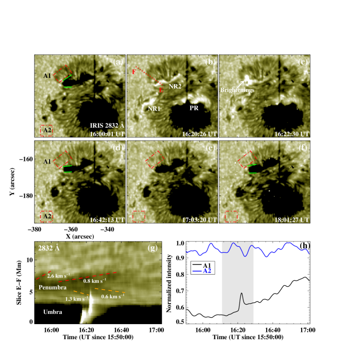
Figure 9: Panels (a)-(f): IRIS 2832 Å images showing the penumbral decay following the X2.1 flare. Areas “A1” and “A2” denote the penumbra and background regions where the intensity-time profiles in panel (h) are calculated. Green lines represent the size of the umbra before and after the flare. Dotted line “E$-$F” (panel (b)) shows the cut position used to obtain the time-distance plot shown in panel (g). Panels (g)-(h): time-distance plot along slice “E$-$F” at 2832 Å and intensity-time profiles within regions “A1” and “A2”. Red dashed lines in panel (g) indicate the penumbra outflow and orange dashed ones indicate the inflow towards the umbra after the flare start. Gray section in panel (h) represents the time interval between the flare start and end.

Figure 9 shows the evolution of the sunspots at the flaring region in IRIS 2832 Å images. One positive-polarity flare ribbon (PR; Figures 7(c) and 9(b)) and two negative-polarity ribbons (NR1 and NR2) were involved in the flare. The ribbon PR extended towards the south at a speed of $\sim$ 8 km s^-1 and swept across a fraction of the main sunspot with a distance of about 2.2 Mm. The ribbons NR1 and NR2 moved in the opposite directions and almost swept across the entire negative-polarity sunspots. Transient spike-like brightenings were observed at the east of NR2 while NR2 swept across the north negative-polarity sunspot (Figure 9(c)). Then the northeast penumbra (area “A1”) started to decay and the penumbral dark fibrils progressively lost their filamentary structure (Figures 9(d)-(f)). Finally the dark fibrils completely disappeared within an hour after the onset of the flare. The size of the umbra region became smaller just after the flare (green lines in Figures 9(a) and (d)). Then the area of the umbra gradually increased during the process of penumbral decay (Figure 9(f)). The time-distance plot along the slice “E$-$F” showed the evolution of penumbral segments after the ribbon NR2 swept across them (Figure 9(g)). Continuous outflow along the penumbral filaments was shown in the time-distance plot (red dashed lines). This outflow had a velocity of 1$-$3 km s^-1, consistent with the typical speed of the Evershed flow (Evershed 1909). After the flare started, the penumbra inflow towards the umbra became evident (orange dashed lines). The inflow had a velocity of about 1 km s^-1 and existed in the early stage of penumbral decay. The 2832 Å emission intensity within the area “A1” was enhanced by about 40 % (black curve in Figure 9(h)). The background region “A2” away from the flare brightenings does not show the flaring time profile seen in “A1” (blue curve in Figure 9(h)).

4 Summary and Discussion

We present the IRIS and the SDO observations of the slipping motion of flux rope structures in the preflare stage on 2015 March 11. The slippage occurred at the north part of the flux rope around the main sunspot of AR 12297. Multiple bright loop structures of the flux rope at 1400 Å and 1330 Å successively slipped toward the east at speeds of about 30$-$40 km s^-1 and seemed to peel off the flux rope. The slippage exhibited a quasi-periodic pattern and the associated period was about 130$\pm$30 s. The IRIS slit crossed the west legs of slipping structures and the spectroscopic observations of the Si iv 1402.77 Å line showed a redshift of about 10$-$30 km s^-1 and a line width reaching 50$-$120 km s^-1. The quasi-periodic slipping motion lasted about 40 min and at the late stage the flux rope started to rise up slowly. Then an X2.1 flare occurred and almost simultaneously, the flux rope was impulsively accelerated. One negative-polarity flare ribbon swept across a small sunspot and the penumbral segments of the sunspot showed an evident decay, with the IRIS 2832 Å emission intensity enhancing by about 40 % in about 50 min. The NLFFF extrapolation results show the existence of a twisted flux rope at the flaring region. The calculated 3D QSL structures are surrounding the flux rope, indicating that the preflare slipping motion is around the flux-rope-related QSLs.

The results suggest that quasi-periodic slipping magnetic reconnection has started in the preflare stage. The Si iv profile was redshifted by 10$-$30 km s^-1 at the legs of slipping structures, probably indicative of reconnection downflows. The topology analysis of the 3D coronal magnetic field structure shows that 3D QSL structures bind the twisted flux rope, separating the flux rope from the surrounding field. The reconnection between the field lines of the flux rope and neighboring field lines continuously occurs along the flux-rope-related QSLs, causing the exchange of field line linkage and the apparent slipping motion of the flux rope structures. The quasi-periodic pattern indicates that the slipping reconnection reappears for multiple times at a certain location, with a regular time interval. The period of the preflare slipping motion varies between 100 and 150 s, averaging $\sim$ 130 s, shorter than that of the slipping flare loops as reported by Li & Zhang (2015) and Li et al. (2015). The quasi-periodic oscillations of the footpoints of slipping flare loops have been reported by Brannon et al. (2015) and Brosius & Daw (2015), who analyzed the same event on 2014 April 18 using the IRIS data. Brannon et al. (2015) presented that the coherent oscillations of small-scale substructure of the flare ribbon have an average period of about 140 s, consistent with our observations. They interpreted that a tearing mode or Kelvin-Helmholtz instability in coronal current sheets drives these oscillations. Another explanation responsible for oscillatory reconnection is related to the relationship between energy load and unload balance (Nakariakov & Melnikov 2009; Brosius & Daw 2015). In these models the magnetic energy is continuously built up through photospheric (shearing and converging) motions until a critical level is achieved resulting in a release of the magnetic energy via reconnection. This process repeats several times with the magnetic energy building up before release.

The flux rope eruption and the X2.1 flare occurred just after the slipping motion of flux rope structures. The long-duration slipping magnetic reconnection at the border of the flux rope probably caused the loss of equilibrium of the flux rope system, and drove the later eruption of the flux rope and the associated flare. Magnetic reconnection at the top border of the pre-eruptive flux rope has rarely been reported. During the eruption process, most models locate the reconnection site in the vertical current sheet below the flux rope. Few observations showed that energy release and reconnection could also occur at the leading edge of an erupting flux rope (Ji et al. 2003; Huang et al. 2011; Jiang et al. 2016). Wang et al. (2009) suggested that EUV brightenings at the far endpoints of erupting filaments were caused by magnetic reconnection at the boundary between the erupting filament and the background corona. The helical current sheet at the interface between a kink-unstable flux rope and the surrounding medium was simulated by Kliem et al. (2004). The reconnection at the border of the flux rope is different from the breakout model proposed by Antiochos et al. (1999) in a closed quadrupolar configuration, although reconnection sites are both overlying the erupting flux rope in the two scenarios. The breakout model involves open fields for the larger-scale connectivity region and the reconnection site is high in the corona. However, the reconnection at the border of the flux rope occurs at a lower altitude.

Our observations imply that the preflare slipping motion of flux rope structures makes the flux rope system unstable, resulting in an eruption. Preflare activities have been considered as a potential clue to understand the triggering mechanism of solar flares, and help to predict the occurrence of solar flares. Previous studies showed that localized brightenings in X-ray, EUV/UV wavelengths and microwave bursts occurred several minutes or more before the onset of the flare (Fárník et al. 1996; Chifor et al. 2007; Zhang et al. 2015b). These preflare brightenings coincided with the presence of emerging or cancelling flux (Joshi et al. 2011). Awasthi et al. (2014) revealed the brightened loop top in 131 Å observations prior to the onset of the precursor phase. Our observations also showed that the preflare brightenings at the loop tops in 1400 Å and 1330 Å channels were more evident. Kim et al. (2001) found a rapid flipping and connectivity change of filament threads in H$\alpha$ images preceding the filament eruption. The magnetic flipping might be associated with the slipping magnetic reconnection in this work. It has been suggested that the pre-flare activities may be a result of slow reconnection and induce the filament eruption and the subsequent flaring (Moore & Roumeliotis 1992; Kim et al. 2001).

The observations of rapid penumbral decay during flares have been reported before (Wang et al. 2004; Deng et al. 2005). It is suggested that flare-related photospheric magnetic field changes make the penumbral magnetic field relaxing upward by rapid magnetic reconnection and becoming more vertical (Sudol & Harvey 2005; Verma & Denker 2012). In our observations, the inflow towards the umbra associated with the penumbral decay was first reported. When the magnetic field lines in the penumbrae turned from more inclined to more vertical, the material of the penumbral filaments flowed towards their footpoints and resulted in the observed inflow towards the umbra. Moreover, the area of the umbra decreased just after the flare and then gradually increased during long-term evolution. The area reduction of the umbra might be caused by the magnetic field topology change during the flare. The later increase in the area of the umbra was probably related to penumbral decay. For the magnetic field lines in the penumbrae became vertical, the penumbrae at the inner edge developed into the umbra that are mainly vertical magnetic flux tubes.

References

- (1) Antiochos, S. K., DeVore, C. R., & Klimchuk, J. A. 1999, ApJ, 510, 485
- (2) Aulanier, G., Démoulin, P., & Grappin, R. 2005, A&A, 430, 1067
- (3) Aulanier, G., Golub, L., DeLuca, E. E., et al. 2007, Science, 318, 1588
- (4) Aulanier, G., Pariat, E., Démoulin, P., & DeVore, C. R. 2006, Sol. Phys., 238, 347
- (5) Awasthi, A. K., Jain, R., Gadhiya, P. D., et al. 2014, MNRAS, 437, 2249
- (6) Bobra, M. G., Sun, X., Hoeksema, J. T., et al. 2014, Sol. Phys., 289, 3549
- (7) Brosius, J. W., & Daw, A. N. 2015, ApJ, 810, 45
- (8) Brannon, S. R., Longcope, D. W., & Qiu, J. 2015, ApJ, 810, 4
- (9) Cheng, X., Ding, M. D., Guo, Y., et al. 2014, ApJ, 780, 28
- (10) Chifor, C., Tripathi, D., Mason, H. E., & Dennis, B. R. 2007, A&A, 472, 967
- (11) Demoulin, P., Henoux, J. C., & Mandrini, C. H. 1994, A&A, 285, 1023
- (12) Demoulin, P., Henoux, J. C., Priest, E. R., & Mandrini, C. H. 1996, A&A, 308, 643
- (13) Demoulin, P., van Driel-Gesztelyi, L., Schmieder, B., et al. 1993, A&A, 271, 292
- (14) Deng, N., Liu, C., Yang, G., Wang, H., & Denker, C. 2005, ApJ, 623, 1195
- (15) De Pontieu, B., Title, A. M., Lemen, J. R., et al. 2014, Sol. Phys., 289, 2733
- (16) Dudík, J., Janvier, M., Aulanier, G., et al. 2014, ApJ, 784, 144
- (17) Dudík, J., Polito, V., Janvier, M., et al. 2016, ApJ, 823, 41
- (18) Evershed, J. 1909, MNRAS, 69, 454
- (19) Fárník, F., Hudson, H., & Watanabe, T. 1996, Sol. Phys., 165, 169
- (20) Forbes, T. G., Linker, J. A., Chen, J., et al. 2006, Space Sci. Rev., 123, 251
- (21) Gorbachev, V. S., & Somov, B. V. 1988, Sol. Phys., 117, 77
- (22) Gosling, J. T., McComas, D. J., Phillips, J. L., & Bame, S. J. 1991, J. Geophys. Res., 96, 7831
- (23) Guo, Y., Ding, M. D., Schmieder, B., et al. 2010, ApJ, 725, L38
- (24) Hood, A. W., & Priest, E. R. 1981, Geophysical and Astrophysical Fluid Dynamics, 17, 297
- (25) Huang, J., Démoulin, P., Pick, M., et al. 2011, ApJ, 729, 107
- (26) Janvier, M., Aulanier, G., Pariat, E., & Démoulin, P. 2013, A&A, 555, A77
- (27) Janvier, M., Aulanier, G., & Démoulin, P. 2015, Sol. Phys., 290, 3425
- (28) Ji, H., Wang, H., Schmahl, E. J., Moon, Y.-J., & Jiang, Y. 2003, ApJ, 595, L135
- (29) Jiang, C., Wu, S. T., Feng, X., & Hu, Q. 2016, Nature Communications, 7, 11522
- (30) Joshi, B., Veronig, A. M., Lee, J., et al. 2011, ApJ, 743, 195
- (31) Kim, J.-H., Yun, H. S., Lee, S., et al. 2001, ApJ, 547, L85
- (32) Kliem, B., Titov, V. S., & Török, T. 2004, A&A, 413, L23
- (33) Lemen, J. R., Title, A. M., Akin, D. J., et al. 2012, Sol. Phys., 275, 17
- (34) Li, D., Ning, Z. J., & Zhang, Q. M. 2015, ApJ, 807, 72
- (35) Li, T., & Zhang, J. 2013, ApJ, 778, L29
- (36) Li, T., & Zhang, J. 2014, ApJ, 791, L13
- (37) Li, T., & Zhang, J. 2015, ApJ, 804, L8
- (38) Li, T., & Zhang, J. 2016, A&A, 589, A114
- (39) Longcope, D. W. 2005, Living Reviews in Solar Physics, 2, 7
- (40) Mandrini, C. H., Demoulin, P., Rovira, M. G., de La Beaujardiere, J.-F., & Henoux, J. C. 1995, A&A, 303, 927
- (41) Mandrini, C. H., Schmieder, B., Démoulin, P., Guo, Y., & Cristiani, G. D. 2014, Sol. Phys., 289, 2041
- (42) Masson, S., Pariat, E., Aulanier, G., & Schrijver, C. J. 2009, ApJ, 700, 559
- (43) Milligan, R. O., & Dennis, B. R. 2009, ApJ, 699, 968
- (44) Moore, R. L., & Roumeliotis, G. 1992, IAU Colloq. 133: Eruptive Solar Flares, 399, 69
- (45) Nakariakov, V. M., & Melnikov, V. F. 2009, Space Sci. Rev., 149, 119
- (46) O’Dwyer, B., Del Zanna, G., Mason, H. E., Weber, M. A., & Tripathi, D. 2010, A&A, 521, A21
- (47) Pariat, E., & Démoulin, P. 2012, A&A, 541, A78
- (48) Pesnell, W. D., Thompson, B. J., & Chamberlin, P. C. 2012, Sol. Phys., 275, 3
- (49) Peter, H., Tian, H., Curdt, W., et al. 2014, Science, 346, 1255726
- (50) Priest, E. R., & Démoulin, P. 1995, J. Geophys. Res., 100, 23443
- (51) Savcheva, A., Pariat, E., van Ballegooijen, A., Aulanier, G., & DeLuca, E. 2012, ApJ, 750, 15
- (52) Savcheva, A., Pariat, E., McKillop, S., et al. 2015, ApJ, 810, 96
- (53) Scherrer, P. H., Schou, J., Bush, R. I., et al. 2012, Sol. Phys., 275, 207
- (54) Schmieder, B., Heinzel, P., van Driel-Gesztelyi, L., & Lemen, J. R. 1996, Sol. Phys., 165, 303
- (55) Shibata, K., & Magara, T. 2011, Living Reviews in Solar Physics, 8, 6
- (56) Sobotka, M., Dudík, J., Denker, C., et al. 2016, arXiv:1605.00464
- (57) Sudol, J. J., & Harvey, J. W. 2005, ApJ, 635, 647
- (58) Sun, X., Hoeksema, J. T., Liu, Y., et al. 2013, ApJ, 778, 139
- (59) Sweet, P. A. 1958, The Observatory, 78, 30
- (60) Tian, H., DeLuca, E., Reeves, K. K., et al. 2014, ApJ, 786, 137
- (61) Titov, V. S. 2007, ApJ, 660, 863
- (62) Titov, V. S., Hornig, G., & Démoulin, P. 2002, Journal of Geophysical Research (Space Physics), 107, 1164
- (63) van Driel-Gesztelyi, L., Hofmann, A., Demoulin, P., Schmieder, B., & Csepura, G. 1994, Sol. Phys., 149, 309
- (64) Verma, M., & Denker, C. 2012, A&A, 545, A92
- (65) Wang, H., & Liu, C. 2012, ApJ, 760, 101
- (66) Wang, H., Liu, C., Qiu, J., et al. 2004, ApJ, 601, L195
- (67) Wang, Y.-M., Muglach, K., & Kliem, B. 2009, ApJ, 699, 133
- (68) Wheatland, M. S., Sturrock, P. A., & Roumeliotis, G. 2000, ApJ, 540, 1150
- (69) Wiegelmann, T. 2004, Sol. Phys., 219, 87
- (70) Wiegelmann, T., Inhester, B., & Sakurai, T. 2006, Sol. Phys., 233, 215
- (71) Wilmot-Smith, A. L., Hornig, G., & Pontin, D. I. 2009, ApJ, 704, 1288
- (72) Yan, X. L., Xue, Z. K., Liu, J. H., Kong, D. F., & Xu, C. L. 2014, ApJ, 797, 52
- (73) Yang, K., Guo, Y., & Ding, M. D. 2015, ApJ, 806, 171
- (74) Zhang, J., Yang, S. H., & Li, T. 2015a, A&A, 580, A2
- (75) Zhang, Y., Tan, B., Karlický, M., et al. 2015b, ApJ, 799, 30
- (76) Zhao, J., Gilchrist, S. A., Aulanier, G., et al. 2016, ApJ, 823, 62
- (77) Zheng, R., Chen, Y., & Wang, B. 2016, ApJ, 823, 136