Interpretation of the cosmic ray positron and antiproton fluxes

Abstract

The spectral shape of cosmic ray positrons and antiprotons has been accurately measured in the broad kinetic energy range 1–350 GeV. In the higher part of this range ($E\gtrsim 30$ GeV) the $e^{+}$ and $\overline{p}$ are both well described by power laws with spectral indices $\gamma_{e^{+}}\simeq 2.77\pm 0.02$ and $\gamma_{\overline{p}}\simeq 2.78\pm 0.04$ that are approximately equal to each other and to the spectral index of protons. In the same energy range the positron/antiproton flux ratio has the approximately constant value $2.04\pm 0.04$, that is consistent with being equal to the ratio $e^{+}/\overline{p}$ calculated for the conventional mechanism of production, where the antiparticles are created as secondaries in the inelastic interactions of primary cosmic rays with interstellar gas. The positron/antiproton ratio at lower energy is significantly higher (reaching a value $e^{+}/\overline{p}\approx 100$ for $E\approx 1$ GeV), but in the entire energy range 1–350 GeV, the flux ratio is consistent with being equal to ratio of the production rates in the conventional mechanism, as the production of low energy antiprotons is kinematically suppressed in collisions with a target at rest. These results strongly suggest that cosmic ray positrons and antiprotons have a common origin as secondaries in hadronic interactions. This conclusion has broad implications for the astrophysics of cosmic rays in the Galaxy.

I Introduction

The study of cosmic ray positrons and antiprotons is a very important topic in high energy astrophysics and has received a very large amount of attention in recent years. A strong motivation for these studies is the possibility that, if the Galactic Dark Matter (DM) is in the form of Weakly Interacting Massive Particles (WIMP’s), the self–annihilation or decay of the DM particles can be an observable source of relativistic antiparticles.

The only known mechanism that can generate a detectable flux of high energy positrons and antiprotons in the Galaxy is their production as secondaries in the inelastic interactions of primary cosmic rays (CR) in interstellar space, or perhaps inside or around the astrophysical sites where CR are accelerated. This conventional mechanism has to be well understood to establish the existence of other contributions generated by alternative mechanisms (such as DM annihilation, or direct acceleration in some classes of astrophysical sources).

The study of the CR fluxes of antiparticles has made a very important step forward thanks to the measurements performed by PAMELA of positrons Adriani:2008zr ; Adriani:2013uda and anti-protons pamela-antiprotons . The PAMELA observation showed that the positron flux, for $E\gtrsim 10$ GeV, is significantly harder than predictions based on the conventional mechanism, and this discrepancy has generated an intense attention and a large body of literature.

The PAMELA results for the positron flux have been confirmed by observations of the FERMI detector FermiLAT:2011ab performed using the Earth magnetic field to separate the fluxes of CR electrons and positrons. More recently the AMS02 detector, on the International Space Station has measured the $e^{+}$ spectrum Aguilar:2014mma , in good agreement with PAMELA, and with smaller errors and extending the observations up to an energy $E\simeq 400$ GeV.

Most of the literature that discusses the CR positron flux takes the point of view that the observations require a new, non–standard source of positrons. Only few works have taken the point of view that the discrepancy between predictions and observations must be attributed to an incorrect estimate of the positron flux generated by the conventional (secondary production) mechanism.

In contrast to the situation for positrons, the measurements of antiprotons performed by PAMELA are consistent with the predictions based on the conventional mechanism of production. This is clearly a very important constraint for the interpretation of the antiparticle data, because many sources of $e^{+}$ are also sources of $\overline{p}$ (and vice–versa). The comparison of positron and antiproton fluxes is therefore crucial to determine the nature and properties of the physical mechanisms that generate antiparticles in the Galaxy.

Recently, the AMS02 collaboration has published a new measurement of the cosmic ray antiproton spectrum. These results are in very good agreement with the PAMELA measurements, but have smaller errors and extend to higher energy (up to $E\simeq 350$ GeV). This allows to determine the shape of the antiproton spectrum with much greater precision.

Having in hands precision measurements of the positron and antiproton fluxes that extend in a broad energy range, together with high quality measurements of the spectra of primary CR particles (protons, electrons and nuclei) allows to perform detailed comparisons that can give important insight about the origin of the different CR components. This work is dedicated to a critical discussion of some intriguing results that emerge from these comparisons.

For energies larger than approximately 30 GeV the spectra of protons, electrons, antiprotons and positrons are well described by power laws ($\phi_{j}(E)\propto E^{-\gamma_{j}}$). It is remarkable that the spectral indices for positrons and antiprotons are consistent with being equal ($\gamma_{e^{+}}\simeq 2.77\pm 0.02$ and $\gamma_{\overline{p}}\simeq 2.78\pm 0.04$), and are also very close to the spectral index for protons. Only the electron flux has a different shape, and is much softer with a larger spectral index of order $\gamma_{e^{-}}\approx 3.2$.

The $e^{+}/\overline{p}$ ratio is approximately constant in the energy range [30–350] GeV with value $2.04\pm 0.04$. This value is also equal (taking into account systematic uncertainties) to the $e^{+}/\overline{p}$ ratio at production for the conventional mechanism. In fact it is possible to show the numerical validity of a stronger result: the observed $e^{+}/\overline{p}$ ratio, is consistent with being equal to the ratio $e^{+}/\overline{p}$ calculated for the conventional mechanism of secondary production, in the entire energy range [1–350] GeV, including the lower energy part where the positron/antiproton ratio changes rapidly with $E$, taking the value $e^{+}/\overline{p}\approx 100$ for kinetic energy $E\approx 1$ GeV.

These intriguing results, are perhaps just a numerical accident but, at least at face value, seem to indicate that the CR fluxes of both positrons and antiprotons have their origin in the conventional secondary production mechanism. This is in contrast to all models where $e^{+}$ and $\overline{p}$ have different origin. This interpretation has however some non trivial difficulties, and requires a deep revision of some important concepts for the formation and propagation of the Galactic cosmic rays. In the following we will attempt to discuss critically these problems.

This work is organized as follows. The next section summarizes recent measurements of the cosmic ray fluxes. Section III discusses the production of positrons and antiprotons in hadronic interactions, and computes the antiparticles production rates in the solar neighborhood. Section IV discusess the energy losses of relativistic particles propagating in the Galaxy. Section V outlines some general concepts about the formation of the CR fluxes in the Galaxy, and describes what can be considered the current (broadly, but not universally accepted) “standard framework” for the study of the Galactic Cosmic Rays. Section VI discusses alternative frameworks for CR in the Galaxy that can explain naturally the correlations between the positron and antiproton fluxes. Section VII contains a short discussion of the significance of the measurements of secondary nuclei. The final section gives a summary and comments of the most promising directions for future studies to clarify the situation. The appendix A discusses an analytic estimate for the ratio $e^{+}/\overline{p}$ at production under the assumption that the antiparticles are generated as secondaries in inelastic hadronic interactions.

II Cosmic Ray fluxes

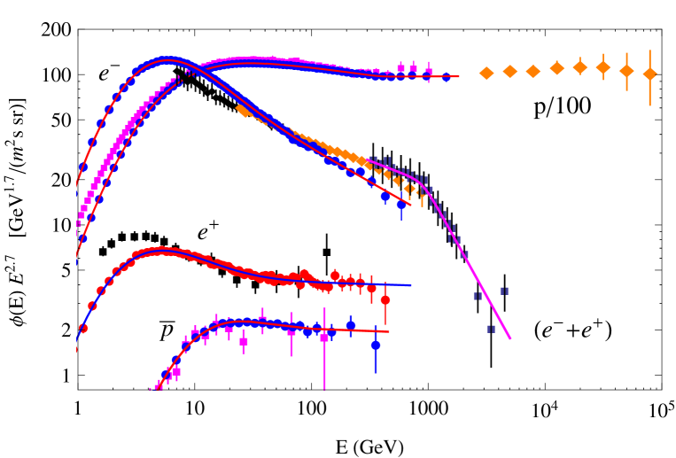
Figure 1: Fluxes of $p$, $e^{-}$, $e^{+}$ and $\overline{p}$. The fluxes are shown in the form $\phi_{j}(E)\;E^{2.7}$ versus $E$ (with $E$ the kinetic energy) to enhance the features of the energy dependence. The proton data (rescaled by a factor $10^{-2}$) is from PAMELA (squares) pamela-protons-helium , AMS02 (circles) ams-protons and CREAM (diamonds) Yoon:2011aa . The electron data is from AMS02 Aguilar:2014mma . The positron data is from PAMELA (squares) Adriani:2013uda and AMS02 (circles) Aguilar:2014mma . The ($e^{-}+e^{+})$ data is from FERMI (diamonds) Abdo:2009zk and HESS (squares) Aharonian:2008aa ; Aharonian:2009ah . The antiproton data is from PAMELA (squares) pamela-antiprotons and AM02 (circles)Aguilar:2016kjl . The lines are fit to the AMS02 data, and to the HESS $(e^{-}+e^{+})$ data

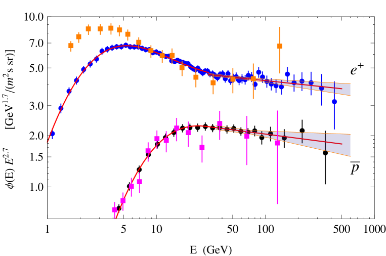
Figure 2: Fluxes of $e^{+}$ and $\overline{p}$ shown in the form $\phi_{j}(E)\;E^{2.7}$ versus $E$. The circles are measurements by AMS02 Aguilar:2014mma , Aguilar:2016kjl . The squares are measurements by PAMELA Adriani:2013uda and pamela-antiprotons . The lines are smooth fits to the AMS02 data. The band indicate the range of power law fits to the AMS02 data in the range $E>30$ GeV (see text).

Recent measurements of the fluxes of protons, electrons, antiprotons and positrons are shown in Fig. 1 in the form $\phi_{j}(E)\times E^{2.7}$ versus $E$ with $\phi_{j}(E)$ the differential energy spectrum for particle type $j$ and $E$ the kinetic energy. The spectra are shown multiplied by the factor $E^{2.7}$ for a better visualization of the spectral shapes, note also that the proton flux is rescaled by a factor $10^{-2}$ The measurements are by PAMELA (for $p$, $\overline{p}$ and $e^{\mp}$) pamela-protons-helium ; pamela-antiprotons ; Adriani:2013uda ; Adriani:2011xv , AMS02 (also $p$, $\overline{p}$ and $e^{\mp}$) ams-protons ; Aguilar:2014mma ; Aguilar:2016kjl CREAM ($p$ at high energy) Yoon:2011aa , FERMI ($e^{+}+e^{-}$) Abdo:2009zk and HESS ($e^{+}+e^{-}$) Aharonian:2008aa ; Aharonian:2009ah . The measurements of the $e^{+}$ and $\overline{p}$ spectra are also shown with an enlarged scale in Fig. 2.

In this work the spectra of different particle types are shown and compared as differential distribution in kinetic energy. This choice is not unique. An equally valid possibility is to show and compare magnetic rigidity spectra at the same (absolute) value of the rigidity. The following discussion about the mechanisms that shape the CR (anti)–particle spectra can be easily reformulated for a different choice of the variable used to represent the observations. Obviously, for particles of unit charge the energy and the (absolute value of the) rigidity become equal in the limit of large $E$ .

Inspecting Fig. 1 and 2 one can make the following remarks:

• The proton flux for $E\gtrsim 30$ GeV has approximately a power law form ($\phi_{p}(E)\propto E^{-\gamma_{p}}$) with an intriguing hardening feature at energy $E\simeq 300$ GeV. The feature was first deduced by CREAM cream-discrepant-hardening , then directly observed by PAMELA pamela-protons-helium and now is also clearly confirmed by the AMS02 data ams-protons . The AMS02 collaboration ams-protons has fitted its measurement of the proton flux as the transition between two power laws with exponents $\gamma_{p}$ and $\gamma_{p}+\Delta\gamma_{p}$ above and below the transition momentum $p^{*}\simeq 336^{+44}_{-26}$ GeV. The best fit values of the parameters are: $\gamma_{p}\simeq 2.849^{+0.006}_{-0.005}$ and $\Delta\gamma_{p}=-0.133^{+0.056}_{-0.037}$.

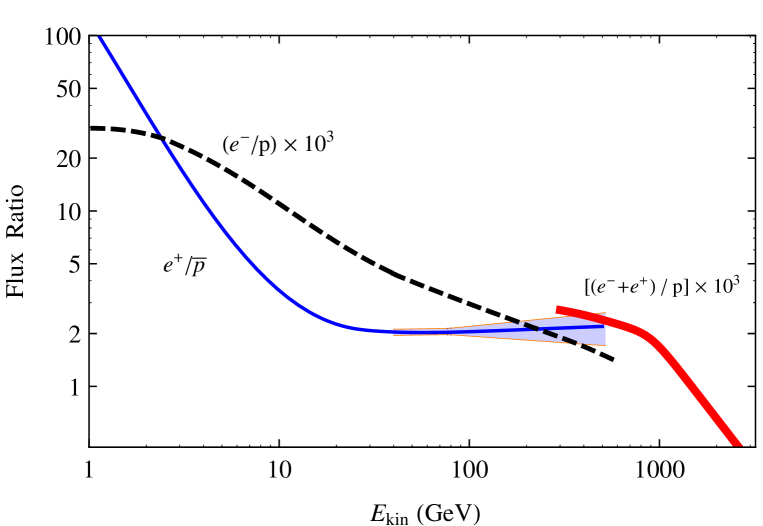
Figure 3: Ratios $e^{+}/\overline{p}$, $e^{-}/p$, and $(e^{-}+e^{+})/p$ between the fluxes of different particle types. All lines are ratios of the fits to the experimental data shown in Fig. 1 and Fig. 2. For the $e^{+}/\overline{p}$ ratio the fit given in equation (4) is also shown.

• The energy spectrum of cosmic ray electrons, is significantly smaller and softer than the corresponding proton spectrum. The ratio $e^{-}/p$ of the electron and proton fluxes is shown in Fig. 3 as a function of the particle kinetic energy $E$. For low energy ($0.5\lesssim E\lesssim 2$ GeV) the ratio $e^{-}/p$ has a value of order 0.03. Increasing $E$ the ratio falls rapidy, and at $E=100$ GeV it is approximately $3\times 10^{-3}$, one order of magnitude smaller. The energy dependence of the ratio in the energy range $E\in[30,300]$ GeV is reasonably well described by a power law:

  $$\left.\frac{\phi_{e^{-}}(E)}{\phi_{p}(E)}\right|_{E\in[30,300]~{}{\rm GeV}}\simeq(3.95\pm 0.10)\times 10^{-3}\;\left(\frac{E}{50~{}{\rm GeV}}\right)^{-0.41\pm 0.02}$$ (1)

• Inspecting Fig. 1 and 2 it is apparent that for kinetic energy $E\gtrsim 20$–30 GeV the spectra of positrons and antiprotons have a shape that is reasonably well approximated by a simple power law. To test this hypothesis, we have fitted the AMS02 data points in the energy range $E>30$ GeV with the functional form:

  $$\phi_{j}(E)=K_{j}\;\left(\frac{E}{50~{}{\rm GeV}}\right)^{-\gamma_{j}}$$ (2)

  (with $j=e^{+}$ or $\overline{p}$). For positrons we obtain a best fit with $\chi^{2}_{\rm min}=12.0$ for 27 degrees of freedom (d.o.f.), and best fit parameters $K_{e^{+}}=(11.4\pm 0.1)\times 10^{-5}$ (m²s sr GeV)^-1 and $\gamma_{e^{+}}=2.77\pm 0.02$. The $\chi^{2}$ of the fit has been calculated summing in quadrature statistical and systematic errors, the resulting value of $\chi^{2}_{\rm min}$ is small, indicating the existence of correlations in the systematic errors for different points. For antiprotons the best fit has $\chi^{2}_{\rm min}=1.56$ for 10 d.o.f. with best fit parameters $K_{\overline{p}}=(5.6\pm 0.1)\times 10^{-5}$ (m²s sr GeV)^-1, and $\gamma_{\overline{p}}=2.78\pm 0.04$.

  It is remarkable that the estimate of the (approximately constant) spectral indices of the positron and anti-proton spectra in the energy range $E\in[30,350]$ GeV are consistent with being equal. It is also intriguing that the spectral indices of the antiparticle fluxes are very close to the spectral index for protons:

  $$\gamma_{e^{+}}\simeq\gamma_{\overline{p}}\approx\gamma_{p}+\frac{\Delta\gamma_{p}}{2}$$ (3)

  In the following we will discuss if these results are a simple coincidence or have a deeper physical explanation.

• The positron/antiproton ratio can be estimated combining the results of the two fits:

  $$\left.\frac{\phi_{eˆ+}(E)}{\phi_{\overline{p}}(E)}\right|_{E\in[30,350]~{}{\rm GeV}}\simeq(2.04\pm 0.04)\times\left(\frac{E}{50~{}{\rm GeV}}\right)^{0.015\pm 0.045}$$ (4)

  that is consistent with a constant value. This result is in striking contrast with the behavior of the $e^{-}/p$ ratio (given in equation (1)) that in the same energy range falls rapidly with energy.

  The energy dependence of the $e^{+}/\overline{p}$ ratio in a broader energy range is shown in Fig. 3. For low kinetic energy the ratio varies rapidly with $E$. At $E\simeq 1$ GeV it is of order 100, and decreases monotonically to reach the approximately constant value of order 2 at $E\simeq 20$–30 GeV.

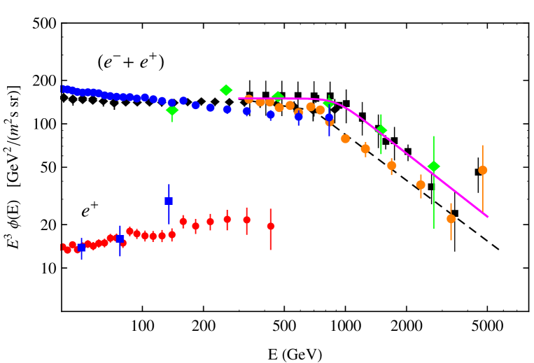
Figure 4: Flux measurements of the sum ($e^{+}+e^{-})$ obtained by AMS02 (small circles) Aguilar:2014fea , FERMI (small diamonds), HESS (squares), MAGIC (diamonds) and VERITAS (big circles). The solid (dashed) line is the best fit to the data obtained by HESS Aharonian:2009ah (VERITAS Staszak:2015kza ).

• Measurements of the spectrum of the sum $(e^{+}+e^{-})$ at very high energy have been obtained by the ground based Atmospheric Cherenkov telescopes HESS Aharonian:2008aa ; Aharonian:2009ah , MAGIC BorlaTridon:2011dk and VERITAS Staszak:2015kza . The results of three Cherenkov telescopes are shown in Fig. 4.

  These results show the existence of a sharp softening of the $(e^{+}+e^{-})$ spectrum at an energy just below 1 TeV. The HESS Collaboration has published a best fit to the data using a broken power with break at energy $E\simeq 900$ GeV, where the spectral index changes from $\gamma_{1}\simeq 3.0$ to $\gamma_{2}\simeq 4.1$ (no errors are reported). The VERITAS Staszak:2015kza ) has also performed a fit using the same broken power law functional form, finding the break at $E\simeq 710\pm 40$ GeV and spectral indices $\gamma_{1}\simeq 3.2\pm 0.1$ and $\gamma_{2}\simeq 4.1\pm 0.1$ (all errors are only statistical). The origin of this very prominent feature remains controversial (see discussion in following).

III Hadronic Interactions and the production of $e^{+}$ and $\overline{p}$

The “normal” mechanism for the production of relativistic positrons and antiprotons is their creation as secondaries in the inelastic interactions of primary cosmic rays with some target material. The leading contribution to this production mechanism is due to $pp$ interaction where one relativistic proton collides with a target proton at rest. Additional contributions are due to helium–proton, proton–helium, helium–helium, $\ldots$ collisions, where different types of CR primary particles interact with different target nuclei. In inelastic hadronic collisions baryon/antibaryon pairs can be created, and after chain decay each antibaryon generates one stable antiproton that enters the CR population. The most abundant source of positrons in hadronic interactions is the creation and chain decay of $\pi^{+}$:

$$\pi^{+}\to\nu_{\mu}+\mu^{+}\to\nu_{\mu}+[e^{+}+\nu_{e}+\overline{\nu}_{\mu}]~{}.$$

The spectrum of the positrons generated in this decay can be calculated exactly using the (non–trivial) matrix element for the 3–body muon decay, and taking into account the fact that the muons created in the first decay are in a well defined polarization state (see for example Lipari:2007su ). A subdominant, but not entirely negligible, source of positrons is the production and chain decay of kaons. Also in this case it is straightforward to compute the positron spectrum generated by the decay of a kaon, summing over all chain decay modes (weighted by the appropriate branching ratios). For example a $K^{+}$ can generate positrons either directly (in the decay mode $K^{+}\to e^{+}\nu_{e}\pi^{\circ}$) or after several chain decay modes (such as in $K^{+}\to\mu^{+}\nu_{\mu}\to e^{+}\ldots$).

The leading ($pp$) contribution to the local production rate (that is the number of particles created per unit time, unit volume and unit energy) of positrons (or antiprotons) can be written explicitely as:

$$q_{pp\to e^{+}(\overline{p})}^{\rm loc}(E)=n_{{\rm ism},p}(\vec{x}_{\odot})~{}\int_{E}^{\infty}dE_{0}~{}n_{p}^{\rm loc}(E_{0})\;\beta\,c\,\sigma_{pp}(E_{0})~{}\left[\frac{dN}{dE}(E,E_{0})\right]_{pp\to e^{+}(\overline{p})}~{}.$$ (5)

In this equation $n_{{\rm ism},p}(\vec{x}_{\odot})$ is the density of protons in interstellar gas in the solar neighborhood, $n_{p}^{\rm loc}(E_{0})$ is the number density of CR protons with energy $E_{0}$ in the vicinity of the Sun, $\beta\,c$ is the proton velocity, $\sigma_{pp}(E_{0})$ is the $pp$ inelastic cross section (for collisions with a proton at rest), and $dN_{pp\to j}/dE$ is the inclusive spectrum of secondary particles of type $j$ in the final state of the collision, calculated allowing the chain decay of all unstable parents. The density in interstellar space is so low that it is safe to assume that all unstable particles decay without suffering energy losses. The integration is over all possible energies of the interacting proton.

The other contributions to the production of $e^{+}$ and $\overline{p}$ (such as $p$–helium or helium–$p$) can be obtained with obvious substitutions.

In the following we will show the results of a complete calculation of the local production rate of positrons and antiprotons, performed integrating numerically equation (5) and the other contributions. The calculation is straightforward and requires three basic elements:

• An estimate of the density (and composition) of interstellar gas in the solar neighborhood.

• An estimate of the fluxes of CR protons and nuclei in the local interstellar medium.

• A model for the properties of inelastic hadronic interactions.

For the density of the interstellar gas we have used the value $n_{\rm ism}=1$ cm^-3 and assumed a standard composition with a helium contribution of 9%.

The CR density in the local interstellar space can be easily related to the flux $\phi_{j}^{\rm loc}(E)$ using the (very good) approximation of isotropy. For example for protons:

$$n_{p}^{\rm loc}(E)=\frac{4\,\pi}{\beta\,c}\;\phi_{p}^{\rm loc}(E)~{}.$$ (6)

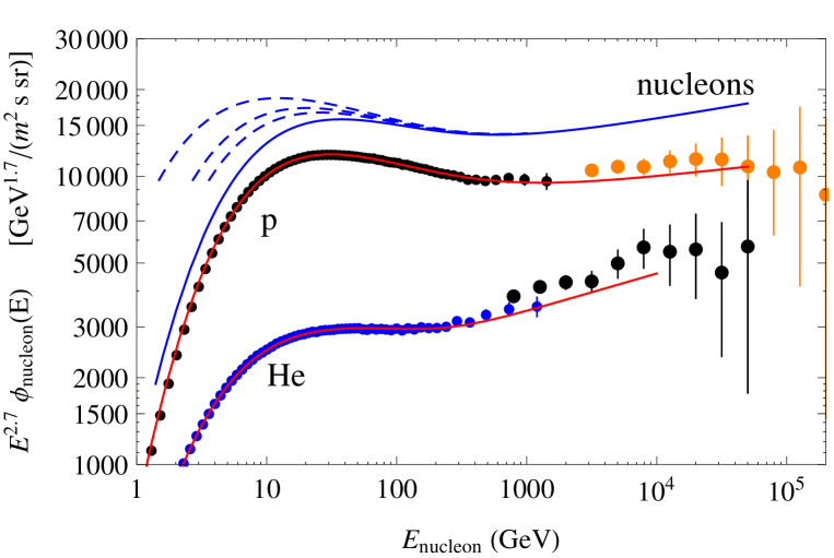
Figure 5: Interstellar spectra for protons and helium used in this work. The data points are measurements performed by AMS02 (small circles) ams-protons ; Aguilar:2015ctt and CREAM (big circles) Yoon:2011aa . The lines show the all nucleon flux at the Earth) solid line and in interstellar space. To correct for solar modulation effects the potential has been estimated as $V=0.4$, 0.6 and 0.9 GV.

A more difficult step is the estimate of the local interstellar spectra from the CR measurements performed near the Earth deconvolving the effects of the (time dependent) solar modulations. The model of the cosmic ray fluxes used in this calculation is shown in figure 5 in the form of the all–nucleon flux versus the kinetic energy per nucleon. The model is based on fits to the AMS02 proton and helium data ams-protons ; Aguilar:2015ctt with a contribution of order 10% from heavier nuclei estimated from the data of the HEAO detector Engelmann:1990zz . At higher energy it joins smoothly with the model of Gaisser, Stanev and Tilav Gaisser:2013bla .

To unfold the effects of solar modulations, we have assumed that the modulations is described by the Force Field Approximation (FFA) Gleeson:1968zza . In the FFA the solar modulations depend on one (time dependent) parameter, the potential $V(t)$. The physical meaning of $V(t)$ is that particles with electric charge $Z$ that penetrate the heliosphere and reach the Earth lose the energy $\Delta E=|Z|\,V(t)$. This is sufficient (using the Liouville theorem) to compute the observable flux at the Earth, and the algorithm can also be inverted analytically Lipari:2014gfa . To take into account theoretical uncertainties we have calculated the CR spectra in the local interstellar space deconvolving the CR measurements shown in Fig. 5 with three values of the potential ($V=0.4$, 0.6 and 0.9 GeV). This gives a non negligible range of uncertainty for primary energies $E\lesssim 50$ GeV. At higher energy the corrections associated to the solar modulations become negligible.

In order to compute the spectra of secondary positrons and antiprotons with an energy as large as $E\simeq 400$ GeV it is necessary to have a description of the primary fluxes up to an energy per nucleon of order 40 TeV. This requires an extrapolation of the measurements performed by the magnetic spectrometers, and requires a modeling of the hardening feature observed at a rigidity of order 250–300 GV. This is an important source of uncertainty.

The final element required for the calculation of the production rates of antiparticles is a model for the inclusive spectra of secondaries in inelastic hadronic interactions. This is probably the main source of systematic uncertainty in the calculation. For a calculation that covers the entire energy range $E\gtrsim 1$ GeV, we have used simple analytic descriptions of the differential cross sections for the production of secondary hadrons in $pp$ interactions constructed on the basis of fixed target accelerator data. For $\overline{p}$ production we have used the parametrization of Tan and Ng Tan:1982nc assuming also that the interactions generate equal spectra of antiprotons and antineutrons. For the production of charged pions we used the parametrizations of Badhwar et al. Badhwar:1977zf , for kaons the work of Anticic et al. Anticic:2010yg .

For a cross check, and to have a first order estimate of the size of the uncertainties we have also performed a calculation, using the Monte Carlo code Pythia (version 6.4) Sjostrand:2006za to obtain numerically the spectra of secondaries. The Pythia code is reliable only at sufficiently high energy, and we have performed this calculation only for (positron and antiproton) energy $E\geq 100$ GeV.

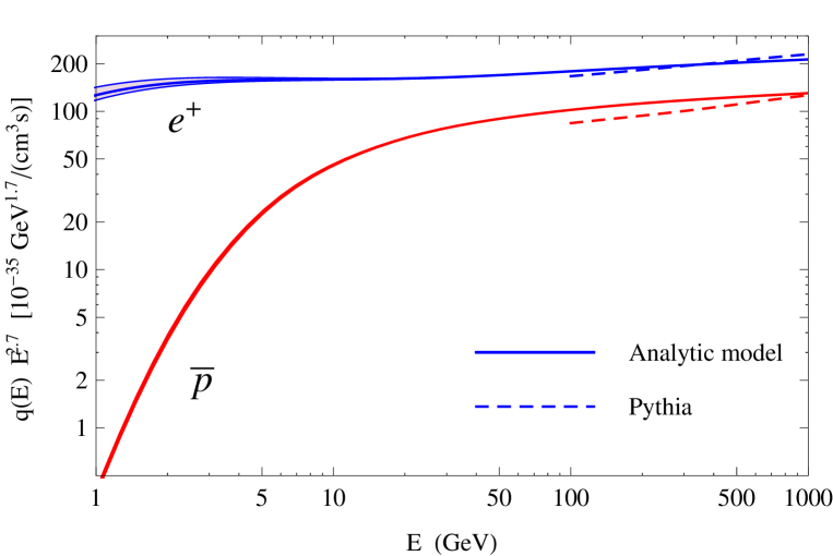
Figure 6: Production rates of $\overline{p}$ and $e^{+}$ calculated with the conventional mechanism in the solar neighborhood. The production rates have been calculated using two methods: an analytic description of the differential hadronic cross sections Tan:1982nc ; Badhwar:1977zf ; Anticic:2010yg , and (for $E>100$ GeV) the Pythia Monte Carlo code Sjostrand:2006za .

The results of the calculation of the local production rates of $e^{+}$ and $\overline{p}$ are shown in Fig. 6. plotted in the form $q_{j}(E)\times E^{2.7}$ versus the kinetic energy $E$ Some interesting features of the numerical results are listed below (in the following of this section we will drop the superscript “loc” in the notation).

1. Uncertainties associated to the description of the solar modulations are significant at low energy, but vanish for $E\gtrsim 20$–30 GeV, when the calculations performed with different value of the potential $V$ become approximately equal.

2. For $E\gtrsim 30$ GeV the spectra of $\overline{p}$ and $e^{+}$ take a simple power law form ($q_{j}(E)\propto E^{-\alpha_{j}}$) with approximately the same exponent.

3. The exponents $\alpha_{e^{+}}$ and $\alpha_{\overline{p}}$ of the positron and antiproton production rates have a value close to the spectral index of the primary proton spectrum:

   $$\alpha_{\overline{p}}\simeq\alpha_{e^{+}}\approx\gamma_{p}~{}.$$ (7)

   This is an expected and well understood result: the energy distributions of secondaries generated by a power law spectrum of primary particles, in good approximation and sufficiently far from threshold effects, have a power law form with the same spectral index (see also discussion below in the appendix A). Note however that equation (7) is not an exact result. This is because the primary spectrum is not a simple power law (and therefore $\gamma_{p}$ is not exactly constant), and scaling violations in the hadronic cross sections also introduce small but non negligible (and model dependent) corrections.

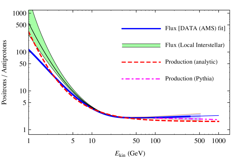
Figure 7: Ratio $e^{+}/\overline{p}$ as a function of the kinetic energy. The thick line shows the ratio $\phi_{\overline{p}}(E)/\phi_{e^{+}}(E)$ of the fluxes observed at the Earth (the line is also shown in Fig. 3). The ratio of the fluxes in interstellar space is shown as a shaded are, and was calculated correcting for the solar modulation effects using three different values of the solar modulation parameter ($V=0.4$, 0.6 and 0.9 GV). The dashed line is the calculated ratio of the production rates of positrons and antiprotons in the solar neighborhood. For $E>100$ GeV also the results of calculation performed using the Pythia Monte Carlo code is shown.

4. The ratio $q_{e^{+}}(E)/q_{\overline{p}}(E)$ of the positrons and antiprotons injection rates is shown in Fig. 7 plotted as a function of the kinetic energy. For small energy the injection rate of positrons is much larger than for antiprotons ($q_{e^{+}}(E)/q_{\overline{p}}(E)\simeq 500$ at $E\simeq 1$ GeV). The ratio decreases monotonically with $E$ and reaches an asymptotic value of order 2 for $E\gtrsim 20$–30 GeV. This behavior can be easily understood qualitatively as a the consequence of simple kinematical effects. The production of antiprotons at low energy is suppressed because the creation of a nucleon/antinucleon pair has a relatively high energy threshold (the minimum kinetic energy of the projectile proton is $E_{0,{\rm min}}=6~{}m_{p}$). In addition the creation of antinucleons at rest or moving backward in the laboratory frame is kinematically forbidden for any projectile energy $E_{0}$. The importance of these kinematical effects becomes progressively less important with increasing energy, and the ratio $e^{+}/p$ converges to an approximately constant value.

   $$\left.\frac{q_{e^{+}}(E)}{q_{\overline{p}}(E)}\right|_{E\gtrsim 30~{}{\rm GeV}}\approx 1.8\div 2.1$$ (8)

   It can be interesting to have a simple analytic calculation of the $e^{+}/\overline{p}$ ratio at production in the limit of high energy (when the ratio is approximately constant). Such a simple calculation allows to discuss an estimate of the different systematic uncertainties. Such a simple calculation is outlined in appendix A.

5. Figure 7 also shows the ratio $n_{e^{+}}(E)/n_{\overline{p}}(E)$ of the densities of antiparticles in the local interstellar medium (estimated deconvolving the effects of solar modulations). The two ratios have energy dependences that are remarkably similar. In fact, taking into account the systematic uncertainties, the two ratios are consistent with being equal in the entire energy range:

   These results can be summarized with the statement:

   $$\frac{\phi_{e^{+}}^{\rm loc}(E)}{\phi_{\overline{p}}^{\rm loc}(E)}\approx\frac{q_{e^{+}}^{\rm loc}(E)}{q_{\overline{p}^{\rm loc}}(E)}~{}.$$ (9)

   an unexpected and intriguing result.

6. The ratio between the local number density and the local injection rate for cosmic rays of type $j$ gives an (energy dependent) characteristic time:

   $$\tau_{j}(E)=\frac{n_{j}^{\rm loc}(E)}{q_{j}^{\rm loc}(E)}\approx$$ (10)

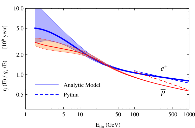
Figure 8: Ratio $n_{j}(E)/q_{j}(E)$ (with $j=\overline{p},e^{+}$) between the measured cosmic ray density and the production rate in the solar neighborhood calculated in the conventional model of secondary production.

   Equation (9) implies that the characteristic times for positrons and antiprotons are approximately equal as shown in Fig. 8. Inspection of this figure shows that the characteristic times are of order 10⁶ years, and have a weak but not trivial energy dependence, most clearly in the low energy region ($E\lesssim 20$–30 GeV). For $E\gtrsim 50$ GeV the energy dependence of the $e^{+}$ and $\overline{p}$ characteristic times is weaker, and a power law description of the numerical results suggests an approximate dependence $\propto E^{0.15\pm 0.07}$, where the error is a rough estimate of the systematic uncertainties associated to the shape of the primary flux and of the modeling of hadronic interactions.

   The quantities $\tau_{j}(E)$ can be related to the residence time of particles in the Galaxy, but the relation depends on the effective volume of the production and containement of the particles.

The result of equation (9) that the ratio of the production rates of positrons and antiprotons in the solar neighborhood, is (within systematic uncertainties) equal to the ratio of the fluxes of $e^{+}$ and $\overline{p}$ is a result that naturally suggests that the local production of antiparticles is representative of the the production rate in the entire Galaxy (or in an important part of the Galaxy), and that the $e^{+}/\overline{p}$ ratio at production is preserved by propagations. It is of course also possible that equation (9) is only a “coincidence”, a numerical accident of no physical significance, and that the positron and antiproton fluxes are generated by distinct source mechanisms. The implications of these two possibilities will be discussed in the following.

IV Energy losses

The rates of energy loss for relativistic $e^{\pm}$ and $p$ ($\overline{p}$) propagating in interstellar space differ by many orders of magnitude. The dominant mechanisms of energy losses are synchrotron emission and Compton scattering (where the target is formed by the radiation fields present in space: CMBR, infrared radiation and starlight). In both cases the rate energy losses depends on the mass and energy of the particles approximately as $|dE/dt|\propto E^{2}/m^{4}$, so that the effect is completely negigible for $p$ and $\overline{p}$, but is potentially important for $e^{\pm}$.

The rate of energy loss of $e^{\mp}$ due to synchrotron radiation is:

$$-\left.\frac{dE}{dt}\right|_{\rm syn}=\frac{4}{3}\;\sigma_{\rm Th}\,c\;\rho_{B}\;\frac{E^{2}}{m_{e}^{2}}$$ (11)

where $E$ is the particle energy, $\rho_{B}=B^{2}/(8\pi)$ is the energy density stored in the magnetic field, and $\sigma_{\rm Th}$ is the Thomson cross section.

The energy loss for Compton scattering depends on the density and energy distribution of the photons that form the target radiation field. In a reasonably good approximation the energy loss of $e^{\mp}$ for Compton scattering is given by an expression very similar to (11):

$$-\left.\frac{dE}{dt}\right|_{{\rm IC}}\simeq\frac{4}{3}\;\sigma_{\rm Th}\,c\;\rho_{\gamma}^{*}(E)\;\frac{E^{2}}{m_{e}^{2}}$$ (12)

where $\rho_{\gamma}^{*}(E)$ is the energy density in target photons that have energy below the maximum value $\varepsilon_{\rm max}\simeq 4\,m_{e}^{2}/E$. This constraint insures that the $e\gamma$ scatterings are in the so called Thomson regime. Interactions with higher energy photons are in the Klein–Nishina regime, where the $e\gamma$ cross section is suppressed.

Combining the energy losses for synchrotron emission and Compton scattering, the characteristic time for energy loss for $e^{\mp}$ is:

$$T_{\rm loss}(E) = \frac{E}{|dE/dt|}\simeq\frac{3\,m_{e}^{2}}{4\,c\,\sigma_{\rm Th}\,\langle\rho_{B}+\rho_{\gamma}^{*}(E)\rangle\;E}$$ (13)

$$\simeq 310.8~{}\left[\frac{\rm GeV}{E}\right]~{}\left[\frac{{\rm eV}\;{\rm cm}^{-3}}{\left\langle\rho_{B}+\rho_{\gamma}^{*}(E)\right\rangle}\right]~{}{\rm Myr}~{}.$$

In this equation the average $\langle\rho_{B}+\rho_{\gamma}^{*}(E)\rangle$ is performed along the trajectory of the particle.

The characteristic time for energy loss scales $\propto E^{-1}$, and depends on the average energy density $\langle\rho_{B}+\rho_{\gamma}^{*}(E)\rangle$. To estimate this energy density one can observe that the energy density of the magnetic field $\rho_{B}=B^{2}/(8\pi)$ scales as the square of the magnetic field, and for $B\simeq 3~{}\mu$G (the typical strength of the magnetic field in the Galactic plane) has the value $\rho_{B}\simeq 0.22$ eV/cm³. The energy density of the radation field can be decomposed in the sum of three main components: CMBR, dust emitted radiation and starlight. The 2.7 Kelvin Cosmic Microwave Background Radiation (CMBR) fills homogeneously all space with the energy density $\rho_{\rm CMBR}\simeq 0.26$ eV/cm³. CMBR photons have the average energy $\langle\varepsilon\rangle\simeq 6.3\times 10^{-4}$ eV, and therefore this component is effective as a target for Compton scattering up to very high energy ($E\lesssim 400$ TeV). The dust emitted infrared radiation in the solar neighborhood has an energy density of order $\rho_{\gamma}\simeq 0.25$ eV/cm³, formed by infrared photons with an average energy of order 0.01 eV, and is effective for $E\lesssim 30$ TeV. Finally starlight in the solar neighborhood has an energy density of order $\rho_{\gamma}\simeq 0.5$ eV/cm³, formed by photons with an average energy of 1 eV, and is effective for $E\lesssim 300$ GeV. One can conclude that the energy loss time of an $e^{\mp}$ with energy of order 1 TeV is of order 0.6 Myr if the particles remain close to the galactic plane, but can also be longer (of order of 1.2 Myr) if the particle confinement volume is much larger than the galactic disk.

V Formation of the Cosmic Ray fluxes

The formation of the Galactic cosmic ray fluxes can be naturally decomposed into two steps: “release” and “propagation”. In the first step, relativistic charged particles are injected or “released” in interstellar space. In the second step the particles propagate in the Galaxy from the release point to the observation point.

Assuming the validity of this decomposition, the relation between $n_{j}(E,\vec{x},t)$ (the density of cosmic rays of type $j$ and energy $E$ present at time $t$ at the point $\vec{x}$) and $q_{j}(E_{i},\vec{x}_{i},t_{i})$ (the rate of release per unit volume of cosmic rays of type $j$ and energy $E_{i}$ at time $t_{i}$ at the point $\vec{x}_{i}$) can be written in general as:

$$n_{j}(E,\vec{x},t)=\int_{-\infty}^{t}dt_{i}~{}\int d^{3}x_{i}~{}\int dE_{i}~{}q_{p}(E_{i},\vec{x}_{i},t_{i})\times P_{j}(E,\vec{x},t;~{}E_{i},\vec{x}_{i},t_{i})~{}.$$ (14)

In this equation $P_{j}(E,\vec{x},t;~{}E_{i},\vec{x}_{i},t_{i})$ is a propagation function that describes the probability density that a particle of type $j$ that at the time $t_{i}$ is at the point $\vec{x}_{i}$ with energy $E_{i}$ can be found at a later time $t$ at the point $\vec{x}$ with energy $E$. The subscript in the notation indicates that the propagation functions will in general have different forms for different particle types.

It is natural to divide the cosmic rays into two classes, according to the nature of their mechanism of interstellar release. Primary particles (such as proton, electrons, or helium nuclei) are accelerated in astrophysical sources and then ejected into interstellar space. Secondary particles (such as the rare nuclei Lithium, Beryllium and Boron) are created already relativistic as final state products in the inelastic interactions of primary cosmic rays.

Equation (14) is written in a very general form, using an absolute minimum of theoretical assumptions: it does not requires that the Galactic CR are in a stationary state, it allows for CR in different points of the Galaxy to have spectra of different shapes, it allows for energy losses or reacceleration during propagation, and leaves the propagation function to have a completely general form. Most models for the Galactic cosmic rays have to introduce several simplifying approximations.

Without loss of generality it is possible to define the current total rate of release of CR of type $j$ as:

$$Q_{j}(E)=\int d^{3}x~{}q_{j}(E,\vec{x},t_{0})~{}.$$ (15)

The flux of CR of type $j$ can be written in the form:

$$\phi_{j}(E)\approx~{}\frac{\beta\,c}{4\,\pi}\;Q_{j}(E)~{}\frac{T_{j}(E)}{V_{\rm eff}}$$ (16)

where $V_{\rm eff}$ is an effective Galactic volume (taken as independent from the particle type and energy), and $T_{j}(E)$ is an (energy dependent) quantity with the dimension of time that has to be calculated constructing a model for CR propagation in the Galaxy. The spectral shapes of CR at the Sun are determined by the combination of two effects: the properties of the sources (that determine of the release spectra), and the properties of propagation.

V.1 The “standard framework” for Cosmic Rays in the Galaxy

In recent years several authors have discussed the problem of the formation of the Cosmic Rays spectra in the Galaxy using a set of very similar ideas and assumptions, that can be seen as constituting a common, broadly (but not universally) accepted framework for the formation of the cosmic ray spectra. We will refer here to this set of ideas and assumptions as the “standard framework” for Cosmic Rays in the Galaxy and outline below some of the most relevant points.

• Relativistic protons and electrons are released in interstellar space by the astrophysical accelerators with energy spectra that, in a broad energy range, have approximately the same shape, so that the $e^{-}/p$ ratio is approximately constant.

  The spectra generated by the accelerators have the same form because the particles are accelerated by a “universal” mechanism, such as Fermi Diffuse Acceleration (DSA), that operates equally on all relativistic charged particles, independently from the sign of the electric charge. The existence of such universal mechanism also insures that the spectra generated by different sources have approximately the same shape (perhaps differing only for having different maximum acceleration energies).

  The difference in mass for electrons and protons results in two important effects. (i) The efficiency for injection in the acceleration mechanism (when the particles are extracted from the tail of thermal distribution of the medium) is higher for protons than for electrons. This results in a (constant) $e^{-}/p$ ratio (for the release spectra) that is much smaller than unity. (ii) The maximum energy that a source can impart to electrons is expected to be smaller than the maximum energy for protons, since it corresponds to the energy for which the rates of acceleration and energy loss are equal.

• The propagation of protons and nuclei is controlled by diffusion generated by the irregular Galactic magnetic field. A fundamental quantity is the residence (or escape) time $T_{\rm esc}(E)$, that is the average time for a cosmic ray to diffuse out of the Galaxy. The escape time is a function of (the absolute value) the particle rigidity, and scales as $\propto\beta^{-1}$.

  The characteristic time for protons or nuclei ($T_{p}(E)$ or $T_{A}(E)$) that enters equation (16) can be identified with the residence time.

• The rigidity dependence of the CR residence time can be determined comparing the spectral shapes of primary and secondary nuclei. The comparison of the spectra of Boron and Carbon suggests the power law dependence:

  $$T_{\rm esc}(p/|Ze|)\propto\left(\frac{p}{|Ze|}\right)^{-\delta}$$ (17)

  with $\delta\simeq 0.4$–0.5.

• The difference in spectral shape between electrons and protons is a propagation effect, and is the consequence of the much larger rate of energy loss for electrons.

• The $e^{-}/p$ ratio start falling for $E$ larger than few GeV. If this is the effect of different energy losses for $e^{-}$ and $p$, one has to infer that for $E\simeq 10$ GeV, the electron residence is longer than the energy loss time (estimated in equation (13)): $T_{\rm esc}(10~{}{\rm GeV})\gtrsim 30$ Myr.

• The characteristic time $T_{e}(E)$ in equation (16) is a combination of the escape time $T_{\rm esc}(E)$ and energy loss time $T_{\rm loss}(E)$. When the loss time is much longer than the residence time ($T_{\rm loss}(E)\gg T_{\rm esc}(E)$) one has $T_{e}(E)\simeq T_{\rm esc}(E)$. In the opposite case ($T_{\rm loss}(E)\ll T_{\rm esc}(E)$) the resulting $T_{e}(E)$ depends on the space distribution of the CR accelerators and the geometry of the CR confinement volume. For example, if the electron release and confinement volumes are identical, one has that $T_{e}(E)\simeq T_{\rm loss}(E)\propto E^{-1}$. If the CR electrons are generated in a disk region much thinner than the confinement volume, then $T_{e}(E)\propto E^{-(1+\delta)/2}$ where $\delta$ is the exponent that describes the energy dependence of $T_{\rm esc}(E)$. More in general the energy dependence of the characteristic electron time can be parametrized with the power law form $T_{e}(E)\propto E^{-\delta_{e}}$ with an exponent $\delta_{e}>\delta$,

  The assumption that electrons and protons are released in interstellar space with the same energy distribution implies that the $e^{-}/p$ ratio measures the different energy dependence of the characteristic times $T_{p}(E)\simeq T_{\rm esc}(E)$ and $T_{e}(E)$:

  $$\frac{\phi_{e^{-}}(E)}{\phi_{p}(E)}\simeq\frac{T_{e}(E)}{T_{p}(E)}\simeq\frac{T_{e}(E)}{T_{\rm esc}(E)}\propto E^{-(\delta_{e}-\delta)}~{}.$$ (18)

• The spectra of CR protons and nuclei are expected to have approximately equal shape in different points of the Galaxy, while the shape of the CR electron spectrum should become softer for points distant from the Galactic plane. This is because the electron accelerators are close to the Galactic plane, and the particles lose a non negligible amount of energy during propagation.

V.2 Antiparticle fluxes in the “standard framework”

Using the chain of arguments outlined above it is possible to estimate the fluxes of positrons and antiprotons generated by the conventional mechanism of secondary production. The result is a predicted positron flux that is significantly softer than the observations.

It is straightforward to present the result stated above for the energy range $E\gtrsim 30$ GeV, where the CR spectra have power law form.

• The spectra of secondary positrons and antiprotons generated in hadronic interactions have approximately the same spectral index as the primary protons (and nuclei):

  $$\alpha_{e^{+}}\simeq\alpha_{\overline{p}}\simeq\gamma_{p}$$ (19)

• The properties of propagation for $e^{+}$ and $e^{-}$ are approximately equal, and similarly for $p$ and $\overline{p}$. This implies that the production spectra of $e^{+}$ and $\overline{p}$ are distorted by the propagation in distinct ways that are predicted by the observations discussed above.

  The prediction for the positron/antiproton ratio is:

  $$\frac{\phi_{e^{+}}(E)}{\phi_{\overline{p}}(E)}\simeq\frac{\phi_{e^{-}}(E)}{\phi_{p}(E)}\simeq\frac{T_{e}(E)}{T_{\rm esc}(E)}\simeq E^{-(\delta_{e}-\delta)}$$ (20)

  Other robust predictions are that positron spectrum should be softer than the electron spectrum, and the $\overline{p}$ should be softer than the $p$ spectrum, with approximately equal distortions:

  $$\frac{\phi_{\overline{p}}(E)}{\phi_{p}(E)}\simeq\frac{\phi_{e^{+}}(E)}{\phi_{e^{-}}(E)}\simeq E^{-\delta}$$ (21)

The predictions presented in equation (20) and (21) are not supported by the data. The most spectacular discrepancy is for the positron flux, that is predicted to be softer than the electron one while in the data the $e^{+}$ spectrum is harder, in direct conflict with the prediction.

In the standard framework for CR in the Galaxy, the hard spectrum of positrons is explained introducing a new source of relativistic positrons (such as direct acceleration in Pulsars or the annihilation or decay of Dark Matter). The shape of the spectrum generated by this new positron source is harder than the spectrum of positrons generated by the conventional mechanism so that, including the softening induced by the propagation, one obtains the observed spectrum.

The new positron source cannot generate a significant spectrum of antiprotons with a spectrum of similar shape, because in the “standard framework” we are discussing here such a new source would result in an antiproton spectrum harder than the positron one, and harder than the observations.

The conclusion is that the observed positron and antiproton fluxes must be generated by distinct mechanisms, and are completely unrelated. The fact that they have the same spectral index ($\gamma_{e^{+}}\simeq\gamma_{\overline{p}}$ for $E>30$ GeV) is just an accident, because these indices emerge in completely different ways. For positrons one has

$$\gamma_{e^{+}}\simeq\alpha_{e^{+}}+\delta_{e}$$ (22)

with $\alpha_{e^{+}}$ the spectral index generated by the new source, and $\delta_{e}$ related to the propagation effect for $e^{\pm}$, while for antiprotons

$$\gamma_{\overline{p}}\simeq\alpha_{\overline{p}}+\delta$$ (23)

with $\alpha_{\overline{p}}$ the spectral index that emerge from the conventional mechanism, and $\delta$ that describes propagation effects for $p(\overline{p})$.

The approximate equality of the spectral indices of positrons and antiprotons is already intriguing, but perhaps even more surprising is the fact that two unrelated mechanisms generate spectra of approximately the same absolute value, in fact that the observed positron/antiproton ratio (approximately $2.04\pm 0.04$) is equal (within systematic uncertainties) to the ratio at production calculated with the conventional mechanism. The last result can in fact be extended to the broader energy range $E\in[1,350]$ GeV, as shown in equation (9), strongly suggesting that we are not in front to a numerical coincidence and that a physical explanation is required.

VI Alternative Framework

In this section we will take the point of view, that the result of equation (9) is not a numerical accident, but is an essential indication that points to a common origin for the observed fluxes of $e^{+}$ and $\overline{p}$, and discuss if this point of view is viable, and what are its implications.

Equation (9) shows that, taking into account statistical and systematic uncertainties, the ratio of the observed fluxes of positrons and antiprotons, is equal to the ratio for the production rate of antiparticles in the solar neighborhood, where the mechanism of production of $e^{+}$ and $\overline{p}$ is the creation of secondaries in the hadronic interactions of primary cosmic rays. If the result is not a simple numerical coincidence, it suggests the following points:

• Secondary production in hadronic interactions is indeed the source of the CR positrons and antiprotons.

• The energy dependence of the “local” (i.e. solar neighborhood) production of antiparticles is representative for the entire (or most of the) production of antiparticles, at least for our space–time point of observation.

• Propagation effects must not distort the energy dependence of the $e^{+}/\overline{p}$ ratio at production. From this one can deduce two results.

  • Positrons and antiprotons must propagate in approximately the same way.

  • The energy of the particles must remain approximately constant during propagation. This is because the $e^{+}$ and $\overline{p}$ production spectra have different shapes, and a significant variation of the energy of the particles during propagation would result in distinct spectral distortions for the two particle types and change the energy dependence of the ratio.

The general expressions for the formation of the spectra of cosmic rays has been given in equation (14). It is possible to express more formally the points just listed above using the same notation. Point (i) and (ii) suggest that the production rates of positrons and antiprotons have the factorized form:

$$q_{e^{+}(\overline{p})}(E,\vec{x},t)\simeq q_{e^{+}(\overline{p})}^{\rm loc}(E)~{}F_{q}(\vec{x},t)$$ (24)

so that the energy dependence of the local production is valid in the region of space and time where the production of antiparticles is important. The function $F_{q}(\vec{x},t)$ that describes the space and time depedence of the antiparticles production must be equal for positrons and antiprotons. This is because, the observed fluxes of $e^{+}$ and $\overline{p}$ are formed summing contributions produced in different points and at different times. To insure that the ratio of the observed fluxes is equal to the ratio at production, the space–time distributions of $q_{e^{+}}$ and $q_{\overline{p}}$ must be equal.

In addition, as stated in point (iii), the propagation of positrons and antiproton must be (approximately) equal, and leave the energy of the antiparticles (approximately) constant. This can be obtained when the propagation functions for positrons and antiprotons in equation (14) take the form:

$$P_{e^{+}(\overline{p})}(E,\vec{x}_{\odot},t_{0};~{}E_{i},\vec{x}_{i},t_{i})\simeq\delta[E-E_{i}]~{}P(E,\vec{x}_{\odot},t_{0};~{}\vec{x}_{i},t_{i})~{}$$ (25)

where $\vec{x}_{\odot}$ is the position of the solar system in the Galaxy, $t_{0}$ the time now, and the function $P$ is equal for positrons and antiprotons.

Inserting equations (24) and (25) in the general expression (14) for propagation one obtains, for the density of positrons and antiprotons at the present time in the vicinity of the Sun the expressions:

$$n_{e^{+}(\overline{p})}^{\rm loc}(E) = q_{e^{+}(\overline{p})}^{\rm loc}(E)~{}\left[\int_{-\infty}^{t_{0}}dt_{i}~{}\int d^{3}x_{i}~{}F_{q}(E,\vec{x}_{i},t_{i})\times P(E,\vec{x}_{\odot},t_{0};~{}\vec{x}_{i},t_{i})\right]$$ (26)

$$= q_{e^{+}(\overline{p})}^{\rm loc}(E)~{}\tau(E)$$ (27)

The factor in square parenthesis in the equation above has the dimension of time, and is common for positrons and antiprotons so that equation (9) is satisfied.

Is it possible to construct a model where the formation of the spectra of positrons and antiproton happens with the properties listed above ? The most critical problem is the requirement that the propagation of positrons and antiproton is (at least approximately) equal. The rates of energy losses for the two particle types differ by many orders of magnitude, therefore the only way to insure that positrons and antiprotons have the same properties in Galactic propagation is that the residence time of the particles in the Galaxy is sufficiently short, so that the total energy loss $\Delta E\simeq|dE/dt|\;T_{\rm esc}(E)$ suffered by positrons during propagation remains negligible ($\Delta E\ll E$). This requirement can also be expressed in the form:

$$T_{\rm esc}(E)<T_{\rm loss}(E)\lesssim 1.2~{}\left[\frac{1}{E_{\rm TeV}}\right]~{}\left[\frac{0.26~{}{\rm eV}\,{\rm cm}^{-3}}{\left\langle\rho_{B}+\rho_{\gamma}^{*}(E)\right\rangle}\right]~{}{\rm Myr}$$ (28)

where we have made use of equation (13). The numerical upper limit on the residence time is obtained setting the energy density $\langle\rho_{B}+\rho_{\gamma}^{*}(E)\rangle$ equal to its minimum value, that is the energy density of the CMBR that permeates uniformly space. This is possible if the confinement volume of the particles is very large, so that the contributions to the energy density of the magnetic field and of radiation generated in the Galaxy (that are concentrated near the Galactic disk) become negligible.

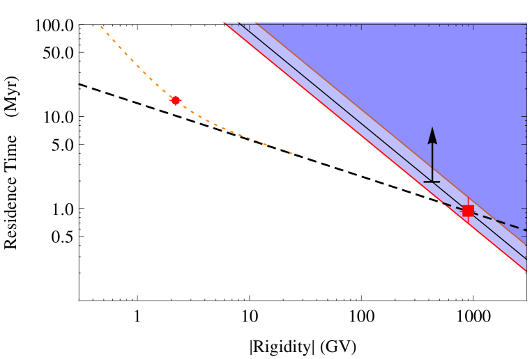
Figure 9: Contraints on the residence time of cosmic rays in the Galaxy. The solid lines are lower limits on $T_{\rm res}$ obtained assuming that positrons with $E\lesssim 430$ GeV suffer neglible energy loss during their residence in the Galaxy. The different lines assume different confinement volumes and therefore different values for the average energy loss rate. The arrow corresponds to the highest energy for which a measurement of the $e^{+}$ flux is available. The point at low rigidity is the estimate on the confinement time $T_{\rm res}=15.0\pm 1.6$ Myr obtained by the CRIS collaboration beryllium3 interpreting their measurement of the ¹⁰Be/⁹Be ratio. The point at rigidity 900 GeV is estimated assuming that the break observed by HESS in the $(e^{+}+e^{-})$ spectrum corresponds to the critical energy where the residence and energy loss time are equal. The dotted line that connects the two points is given by expression (29) with the parameters $T_{0}\simeq 14.0\pm 0.4$ Myr and $\delta\simeq 0.40\pm 0.04$.

The upper bound on the CR residence time in equation (28) is shown graphically in Fig. 9. Is such a bound compatible with existing observations? The most direct and reliable method to estimate the residence time of cosmic rays in the Galaxy is based on the study of the ratio of the beryllium isotopes ¹⁰Be and ⁹Be. Both isotopes are formed as secondaries in the fragmentation of higher mass nuclei, but the beryllium–10 is unstable with an half–life of $1.51\pm 0.04$ Myr Tilley:2004zz and acts as a cosmic–clock to measure the time elapsed from the nucleus creation beryllium1 ; beryllium2 ; beryllium3 . The Cosmic Ray Isotope Spectrometer (CRIS) collaboration, using an instrument aboard the Advanced Composition Explorer (ACE) spacecraft has measured the ratio ¹⁰Be/⁹Be in the energy range $E_{0}\simeq 70$–145 MeV/nucleon (with $E_{0}$ the kinetic energy per nucleon). The ratio is of order 0.11–0.12, and since the production rate of the two isotopes in the fragmentation of higher mass nuclei is approximately equal, this indicates that approximately 90% of the Beryllium–10 nuclei have decayed. The CRIS collaboration, using a a “Leaky Box” theoretical framework has then estimated a residence time $T_{\rm esc}=15.0\pm 1.6$ Myr for the unstable nuclei.

In order to extrapolate these results to $e^{\pm}$ in the energy range of several hundred GeV, one can make the ansatz that the residence time depends on the rigidity and velocity of the particles with the (2–parameter) functional form:

$$T_{\rm res}\approx\frac{T_{0}}{\beta}\;\left(\frac{p}{p_{0}\;|Ze|}\right)^{-\delta_{T}}~{}$$ (29)

($p_{0}$ is an arbitrary scale that without loss of generality can be set to 1 GeV). The constraint that the residence time is shorter than $T_{\rm loss}(E)$ for $E\lesssim E^{*}$ can then be used to set limits on the parameters $\delta_{T}$ and $T_{0}$.

An intriguing possibility is to interpret the spectral break observed by the Atmospheric Cherenkov telescopes as the transition from the regime where the residence time for $e^{\pm}$ is shorter than the loss time, to the regime where the opposite is true. Defining the critical energy $E^{*}$ as the energy where the residence and loss time for $e^{\mp}$ are equal:

$$T_{\rm loss}(E^{*})\simeq T_{\rm res}(E^{*})~{}$$ (30)

one expects to observe a spectral feature in correspondence of $E^{*}$ with a $\Delta\gamma$ that can be as large as unity.

Tentatively identifying the break energy observed by HESS, MAGIC and VERITAS with the critical energy $E^{*}$, one can estimate the residence time for $e^{\mp}$ at the break energy, as it is equal to the loss time. The result (using the HESS estimate for the energy of the break energy):

$$\ T_{\rm res}(900~{}{\rm GeV})\simeq T_{\rm loss}(900~{}{\rm GeV})~{}\simeq 1.0\pm 0.4~{}{\rm Myr}$$ (31)

where the error was estimated taking into account a 20% uncertainty in the energy scale, and a range of possible values for $\langle\rho_{B}+\rho_{\gamma}^{*}\rangle$ in equation (13).

Combining the two measurements of the CR residence time obtained at different rigidities, performed by CRIS using the beryllium ratio beryllium3 , and by the Air Cherenkov telescopes, and comparing to equation (29), one can estimate the two parameters $T_{0}$ and $\delta_{T}$ obtaining the results: $T_{0}\simeq 14.0\pm 0.4$ Myr and $\delta\simeq 0.40\pm 0.04$. The rigidity dependence of the residence time obtained in this estimate is actually consistent with the indications obtained from the ratio $q_{j}^{\rm loc}(E)/n_{j}^{\rm loc}(E)$ discussed in section III and shown in Fig. 8.

The short CR residence time estimated above is also an important constraint in construction of a model of the Galactic magnetic field, since the outflow of the CR particles from the Galaxy (that is inversely proportional to the residence time) must generate, angular anisotropies smaller than the experimental upper limits. Simple diffusive models (see for example Hillas:2005cs ) overpredict the dipole amplitude of the CR angular distribution, and a shorter lifetime exacerbates this problem. It is therefore necessary to go beyond these simple models Mertsch:2014cua ; lipari-anisotropy .

The tentative conclusion we obtain from the discussion outlined above is that an interpretation of the positron and antiproton flux as entirely of secondary origin is in fact viable, and also offers a simple and attractive interpretation for the softening of the $e^{\pm}$ spectrum observed by the Cherenkov telescopes.

The hypothesis that the positron and anti–proton fluxes are of secondary origin has been explored in the past by several other authors see for example Cowsik:2010zz ; Cowsik:2013woa ; Cowsik:2015yra ; Katz:2009yd ; Blum:2013zsa ; Ahlen:2014ica ). An important difference of the present paper with respect to previous works is that here the discussion on the anti–particles fluxes is constructed without making use of the data on secondary nuclei, a topic that will be addressed in the next section.

In the present paper we do not have the space for a critical review of the the work of the authors that have discussed the anti–particles in cosmic rays as secondary products. We would like however to make a brief comment on the work of Blum, Katz and Waxman (BKW) Katz:2009yd ; Blum:2013zsa . These authors conclude that both positrons and anti–protons are of secondary origin, but also rgue that energy losses play a significant role in $e^{+}$ propagation. BKW introduce an energy loss suppression factor $f_{s,e^{+}}(E)$, defined as the ratio between the observed positron flux and the theoretical flux calculated neglecting energy losses, and estimate a value $f_{s,e^{+}}(E)\approx 1/3$ at $E\simeq 20$ GeV. According to BKW the quantity $f_{s,e^{+}}(E)$ grows with energy, approaching the maximum possible value of unity for $E\simeq 300$ GeV. This means that the importance of the energy loss effects in shaping the positron spectrum decreases at higher energy . This behavior is surprising since the $e^{\pm}$ energy losses grow approximately quadratically with $E$. A factor $f_{s,e^{+}}(E)$ that grows with energy requires that positrons of different $E$ remain confined in regions of space that are not identical and contain on average a different magnetic field and a different energy density in radiation (see Eq. (13)) to reduce the energy losses for particles of higher $E$. It is far from easy to construct a satisfactory model to explain the energy dependence of $f_{s,e^{+}}(E)$ along these lines.

In contrast in this work we find find that the comparison of the positron and anti–proton spectra suggests that the $e^{\pm}$ energy losses effects are negligible in the entire energy range where data is available, and therefore, using the notation of BKW, that $f_{s,e^{+}}(E)\simeq 1$ for all energies below the critical energy $E^{*}$ that has been tentatively identified as the energy (of order 900 GeV) where the Cherenkov telescopes observe a spectral break in the ($e^{-}+e^{+}$) spectrum. The origin of the discrepancy between this work and the results of BKW can likely be attributed to a more precise modeling of inelastic hadronic interactions in this work.

VII Secondary Nuclei

A cornerstone of the theoretical studies based on the “standard framework” for the propagation of Galactic cosmic rays is the interpretation of the measurements of “secondary nuclei” such as Lithium, Beryllium and Boron. These nuclei are very rare in ordinary matter, but they are relatively abundant in cosmic rays, because they can be created, already relativistic in the Galaxy rest frame, as secondary products in the fragmentation of higher mass nuclei (mostly Carbon and Oxygen).

The ratio between the fluxes of secondary and primary nuclei can then be interpreted, using fragmentation cross sections measured in laboratory, and correcting for absorption effects, to estimate the average, rigidity dependent column density $X(|p|/Z)$ crossed by the relativistic nuclei.

The best measured quantity to perform this study is the Boron/Carbon (B/C) ratio, and several authors Engelmann:1990zz ; deNolfo:2006qj ; Ahn:2008my ; Obermeier:2012vg ; Adriani:2014xoa have measured and interpreted this ratio. The estimated average column density at a rigidity of few GV is of order of $\approx 5$ g/cm², and decreases with a power law dependence: $X(|p|/Z)\propto(|p|/Z)^{-\delta}$, with an exponent of order $\delta\simeq 0.3$–0.5.

In the “standard framework” for CR Galactic propagation one makes two additional assumptions:

• The column density estimated from the B/C ratio, applies not only to the nuclei that enter the Boron production process, but also to all cosmic rays species, including protons and helium nuclei.

• The column density $X$ crossed by cosmic rays is integrated during their propagation in interstellar space, and therefore it is proportional to the particles Galactic residence time $T$:

  $$X\simeq\langle\rho\rangle\;T$$ (32)

  (where $\langle\rho\rangle$ is the density of the interstellar medium averaged over the particles trajectories).

Using these assumptions it is possible to estimate the spectral shape of the primary cosmic rays as they are released in interstellar space by the Galactic sources, and to construct predictions for the spectra of secondary antiparticles ($e^{+}$ and $\overline{p}$) that are created in the inelastic interactions of (mostly protons and helium nuclei) primary cosmic rays.

The spectrum of secondary positrons constructed as outlined above is very soft, in strong disagreement with the observations. The softness of the $e^{+}$ spectrum is the consequence of the fact that the estimated CR residence time (that also depends on the estimate of $\langle\rho\rangle$, and therefore on the CR confinement volume) is sufficiently long so that the energy losses for $e^{\pm}$ are important. As already discussed, this conflict between predictions and observations is commonly solved introducing a new source of relativistic positrons.

The predictions of the spectrum of high energy antiprotons constructed starting from the B/C ratio, are closer to the observations, but also in this case there is significant tension (if not in open conflict) between predictions and data. In fact, all such predictions of the secondary antiprotons spectrum constructed before the release of the AMS02 data, have obtained results significantly softer than for protons. For example, in the work of Donato et al. Donato:2008jk (inspecting figure 3) the $\overline{p}/p$ ratio for $E\gtrsim 50$ GeV has an energy dependence well described by a power law ($\propto E^{-\alpha}$) with an exponent $\alpha$ in the range $\alpha\approx 0.49\pm 0.05$. In the work of Trotta et al. Trotta:2010mx the energy dependence $\overline{p}/p$ ratio is accurately described (in the same energy range) as a power law with exponent $\alpha\simeq 0.30$. These results can be easily understood qualitatively observing that in these calculations the spectral index of the $\overline{p}$ spectrum, in first approximation, takes the value:

$$\gamma_{\overline{p}}\simeq\gamma_{p}+\delta$$ (33)

where $\gamma_{p}$ is the spectral index of the proton flux, and $\delta$ is the exponent of the power law rigidity dependence of the B/C ratio, that (in the framework in consideration) also give the rigidity dependence of the cosmic ray confinement time. In contrast the measurements performed by AMS02 show spectra of $p$ and $\overline{p}$ that have approximately the same energy dependence.

After the publication of the AMS02 results, several authors (for example Giesen:2015ufa ; Evoli:2015vaa ) have presented revisions of their calculations of of the antiproton flux that also include estimates of the systematic uncertainties in the calculation (the dominant ones are the description of the hardening of the cosmic ray spectra at high rigidity, and the modeling of antiproton production in inelastic hadronic interactions). These authors argue that, taking into account for these uncertainties, their models (based on the “standard framework”) can be reconciled with the AMS02 data. It should be noted however, that also in these “a posteriori” revised calculations, the central value of the prediction for the $\overline{p}/p$ ratio falls with energy. In the work of Giesen et al Giesen:2015ufa the energy dependence of the “best fit” prediction for the $\overline{p}/p$ ratio (in the range $E\gtrsim 50$ GeV) has a power law form ($\propto E^{-\alpha}$) with an exponent $\alpha\simeq 0.28$. In the calculation of Evoli et al. Evoli:2015vaa the ratio falls with energy with an exponent $\alpha\simeq 0.21$. A detailed discussion of this important problem is beyond the scope of this work, but we can observe that while the inclusion of the systematic uncertainties does mitigate the significance of a possible discrepancy between data and prediction, in our view, significant tension remains.

In the present work we are taking a completely different approach, where the origin of the fluxes of positrons and antiprotons in cosmic rays is studied comparing the two antiparticles spectra with each other and with the spectra of the parent particles (protons and helium nuclei), without any input from the observations of secondary nuclei. As discussed above, this study does suggest a common secondary origin for antiparticles. In this approach the ratio of the observed spectra and the spectra generated in the inelastic collisions of the primary particles allows to estimate (see Eq. (10)) an energy (or rigidity) dependent characteristic time for positrons and antiprotons that can be compared to the column density infered from the B/C ratio, effectively reversing the method used in the studies that start with a discussion of the data on secondary nuclei.

The characteristic times for antiprotons and positrons obtained from Eq. (10) appears to fall less rapidly at high energy (or rigidity) than the confinement times estimated from the B/C ratio. This naturally raises the question of how it is possible to reconcile these apparently conflicting results. A complete discussion of this problem is beyond the scope of this paper, it is however appropriate to include here some comments.

The most important discrepancy is about the prediction of the positron spectrum. The study performed here suggests that the energy losses of $e^{\mp}$ are negligible, but this is possible only if the CR confinement time is sufficiently short. The simplest way to reconcile a short CR Galactic residence time with the column density estimated from the B/C ratio is to “disconnect” the two quantities, so that Eq. (32) is not valid. This “disconnection” is possible if most of the column density is integrated inside (or in the envelope) of the sources. In fact, the column density crossed by a relativistic particle can be decomposed into the sum: $X\simeq X_{\rm source}+X_{\rm ism}$ where the first term is accumulated inside or close to its source and the second one is integrated during propagation in interstellar space. The possibility that the $X_{\rm source}$ contribution is dominant in most (or all) the rigidity range where data is available has been extensively discussed by Cowsik, Burch and Madziwa–Nussinov Cowsik:2010zz ; Cowsik:2013woa ; Cowsik:2015yra in the framework of the “Nested Leaky Box Model”.

A second question is then if the hypothesis that all cosmic rays traverse the same (rigidity dependent) column density, equal to what is estimated from the B/C ratio, results in spectra of secondary positrons and antiprotons that are consistent with the observations. In fact, the assumption of the same power law dependence estimated from the B/C ratio for the column density traversed by protons and helium nuclei results in antiparticle spectra that are too soft, because the contributions of lower (higher) energy primaries is relatively enhanced (suppressed), and therefore on predictions that are inconsistent (or at least in strong tension) with the observations. A possible solution for this problem is to modify the rigidity dependence of the column density for high $|p|/Z$. It should in fact be noted that the predictions of the $e^{+}$ or $\overline{p}$ spectrum at energy $E$ requires to sum the contributions of all primary particles with energy $E_{0}>E$, with most of the secondary particles created by primaries with $E_{0}/E$ in the range 10–100. This implies the calculation of the spectra of antiparticles at high energy requires an extrapolation of the estimates infered from the B/C ratio. Cowsik, Cowsik, Burch and Madziwa–Nussinov Cowsik:2010zz ; Cowsik:2013woa ; Cowsik:2015yra have argues that the power law rigidity dependence of the column density infered by the Boron/Carbon ratio is only valid for $|p|/Z\lesssim 200$–300 GV, while for higher rigidities the column density becomes approximately constant. This behavior reflects the transition from a (low rigidity) regime where the column density $X$ is dominated by a power law dependent $X_{\rm source}$ component, to a (high rigidity) regime where an approximately constant interstellar contribution $X_{\rm ism}$ is dominant. A model of this type can possibly generate secondary spectra consistent with the observations, and with the results obtained here and shown in fig. 8.

It is also very desirable to confirm the results obtained with the study of Boron using other secondary nuclei (in particular Lithium and Beryllium). Recently the AMS02 collaboration ams-days-lithium has presented preliminary measurements of the CR Lithium flux that show a striking hardening of the spectrum at a rigidity of order 300 GV, where the spectral index changes with $\Delta\gamma\simeq 0.5$–0.6. This is a spectral feature close the one predicted by Cowsik and collaborators, however the recently published AMS Boron data Aguilar:2016vqr do not exhibit a similar hardening, and appear consistent with a simple power law, in contrast to to Cowsik et al. prediction. These results are surprising, because it is expected that the Boron and Lithium spectra, having the same origin, should have very similar shapes, and a consistent interpretation of the data appears therefore problematic, and a more complete critical discussion on secondary nuclei will be therefore postponed to wait for the publication of the AMS02 measurements also for Lithium and Beryllium.

It should also be stressed that the interpretation of the data on Boron (and of other secondary nuclei) depends crucially on the measurements (see for example Tomassetti:2015nha ), of the fragmentation cross sections of light nuclei in reactions such as ${}^{12}{\rm C}+p\to({}^{10}{\rm B}+p+n)+p$, and in fact on the extrapolation to higher energy of the available data. An unexpected energy dependence of the relevant fragmentation cross sections could have a very significant effect on the interpretation of the data. Given the importance of this question, it is clearly very desirable to obtain new experimental measurements in a more extended energy range.

A final comment is that the hypothesis that the average column density traversed by cosmic rays is equal for all particle types, and in particular is equal for light nuclei (such as Carbon and Oxygen) and for protons and Helium nuclei (that are the main source of antiparticles)is not necessarily correct. The hypothesis is natural if most of the column density is integrated in interstellar space, since the trajectory of a particle is essentially determined only by its magnetic rigidity. On the other hand, if most of the column density is accumulated inside of near a source, and if the dominant sources for different particle types do not coincide, then it is possible that, for the same rigidity, particles of different type traverse a different average $X$. In this case the results obtained for secondary nuclei cannot be applied to the prediction of the antiparticle spectra.

To conclude this brief discussion on secondary nuclei, we can note that this important question certainly deserves a more extended and detailed discussion that will be postponed to a future paper. Given the complexity of this problem, we find that the approach followed in the present work, to tentatively explore the hypothesis of a secondary origin of antiparticles in cosmic rays without including an interpretation of the data on secondary nuclei has its merits. Eventually of course a successful theory should be able to give a satisfactory explanation for all CR data.

VIII Outlook

In this work we have shown and discussed the existence of some surprising properties of CR positrons and antiprotons. The ratio $e^{+}/\overline{p}$ of the antiparticles fluxes falls monotonically with energy from a value of order 100 for kinetic energy $E\simeq 1$ GeV, to a value of approximately two for $E\simeq 25$ GeV, and then remains approximately constant at the value $2.04\pm 0.04$ in the energy interval 30–350 GeV (up to the highest energy of the observations). This is exactly the same behaviour of the ratio $e^{+}/\overline{p}$ for the production rates of antiparticles calculated using the conventional mechanism where $e^{+}$ and $\overline{p}$ are created as secondary products in the inelastic interactions of primary cosmic rays.

Many models for the CR antiparticles claim that the positrons are generated by a new source, that is distinct and unrelated to the (conventional) mechanism that generates antiprotons. If this interpretation is correct, then the results described above have to be considered as numerical accidents of no physical significance.

The alternative is to construct a model where positrons and antiprotons are generated by the conventional mechanism, and where the $e^{+}/\overline{p}$ ratio at production is preserved during propagation. In this paper we have shown that this second possibility is viable, and implies that the CR residence time for $p$, $\overline{p}$ and $e^{\mp}$ is of order 0.6-1.2 Myr at energy $E\simeq 1$ TeV. This interpretation also suggests that the break in the ($e^{+}+e^{-}$) spectrum observed by the Atmospheric Cherenkov telescopes corresponds to the critical energy where the residence time and the loss time for CR $e^{\mp}$ are equal.

Several authors (see for example Yuksel:2008rf ) have discussed models where the hard positron spectrum has it origin in the presence of a near source of particles, in order to avoid the effects of energy losses. These class of solution do not really address in a satisfactory way the puzzle that we are discussing in this work, where the key observations is the close relation between the positron and the antiproton fluxes. To preserve the ratio $e^{+}/\overline{p}$ at production for the flux, the space distribution of the sources of the two particles must be approximately equal. A local source of secondary positrons and antiprotons can be a viable solution but only if it accounts for most of the fluxes for both particles. If antiprotons can reach the Sun from large distances and positrons (because of large energy losses) cannot, this would change the ratio at production, unless the contribution from all distant sources is negligible for both antiparticle types.

In the energy range considered in this work, the CR electron spectrum is much softer than the proton one. This difference in spectral shape is commonly understood as the consequence of different propagation properties for the two particle types that generate different distortions on $p$ and $e^{-}$ spectra that are released in interstellar space by the CR accelerators with approximately the same shape. This interpretation is not possible if the Galactic residence time of the CR particles is sufficiently short so that electrons (and positrons) lose only a small amount of energy inside the Galaxy. In this situation propagation in the Galaxy is entirely controled by magnetic effects and does not depend on the particle mass. In this scenario, to explain the observed difference in spectral shape between high energy electrons and protons, it is necessary to conclude that the CR accelerators release in interstellar space populations of relativistic $p$ and $e^{-}$ that have significantly different spectral shapes.

It should be stressed that the hypothesis that the CR sources generate different spectral shapes for protons and electrons does not necessarily imply that the acceleration mechanism is not “universal” (i.e. only rigidity dependent for ultrarelativistic particles), but it has important implications for the structure and time evolution of the sources, since it requires that energy losses (during or after acceleration) must play an important role, distorting the spectra of the particles that are released in interstellar space. As an analogy, one can think about the Milky Way, seen as a single accelerator that releases in intergalactic space populations of protons and electrons that have very different spectral shapes. In the standard framework, this difference is attributed to the effects of the energy losses on electrons during their propagation in interstellar space, while one fundamental acceleration mechanism creates spectra of electrons and protons that have the same energy distributions. Similarly one can speculate that energy losses inside individual sources (such as supernova remnamnts) can distort the spectra of electrons generated by the acceleration mechanism, so that the relativistic $e^{-}$ and $p$ accelerated by the source, that reach interstellar space have different energy distributions.

The important conclusion is that the interpretation of the CR positrons as secondaries has implications of profound importance about the properties of the Galactic CR accelerators, because it requires that these accelerators generate spectra of protons and electrons of different shape. This suggests (and in fact requires) a program of detailed theoretical and observational studies to test the hypothesis.

In summary, the identification of the mechanisms that generate the CR positrons and antiprotons is intimately tied to the problem of establishing the properties of Galactic propagation for relativistic particles, and to the problem of the determination of the source spectra generated by the Galactic accelerators. Several lines of experimental studies have the potential to contribute to the solution for these problems:

• The simplest idea is to extend the measurements of the positron and fluxes to a broader energy range. If the hypothesis that the positrons have a secondary origin is correct, then the two spectra should exhibit the same spectral softening feature. This spectral break has been already observed by the Cherenkov telescopes in the combined spectrum of ($e^{-}+e^{+}$) at $E\simeq 900$ GeV (where the flux is dominated by electrons). In the standard framework the shape of the positron spectrum is determined by the properties of the new source and can have a variety of different shapes.

• If the hypothesis that the positrons have a secondary origin is correct, the space distributions of protons, electrons and positrons should have approximately equal shapes. This is because the energy losses during propagation should be of negligible importance for all three particle types, and the space distribution of the sources for the three particle types are similar (but not identical).

  In the standard framework, where the energy losses of $e^{\mp}$ are important the space distributions of protons than for electrons, and the shape of the $e^{-}$ energy spectra should be different in different Galactic regions (with softer spectra for points away from the Galactic disk).

  Information about the density and spectral shape of CR $p$ and $e^{\mp}$ in the Galaxy can be obtained from a study of the angular and energy distribution of the diffuse gamma–ray flux FermiLAT:2012aa , and also from the mapping of the radio emission. The reconstruction of the energy and space distributions of CR particles (protons and $e^{\mp}$) in the Galaxy is not an easy task, and requires a sufficiently accurate understanding of the distributions of matter, radiation and magnetic field in the Galaxy, but has great potential.

• If the cosmic ray positrons are of secondary origin, it is necessary to conclude that the CR sources release in interstellar space protons and electrons spectra that have very different spectral shapes. This possibility, at least in principle, can be verified (or falsified) by observations.

  The prospects to obtain soon useful measurements are perhaps most attractive if the CR sources are indeed SuperNova Remnants. Multi–wavelength studies of young SNR’s in our Galaxy have the potential to give valuable information on the size and shape of the spectra of relativistic particles of different type that the sources release in interstellar space. This is a very difficult task that requires taking into account the fact that the observations can study only a relatively small number of objects each having a different age and a different environment.

As a final remark, we would like to note that this paper, in contrast to others, does not claim to have established what is the origin of positrons and anti–protons in cosmic rays, but consider that this remains an open problem of fundamental importance. The CR community is in confronting two alternative models for the origin of CR positrons:

• In the most commonly accepted framework to describe Galactic cosmic rays, where the Galactic accelerators create spectra of electrons and protons that have approximately the same shape in a broad range of energy, it is inevitable to postulate the existence of a new (yet unidentified) hard source of positrons. It is however rather extraordinary that the new source generates an $e^{+}$ spectrum that, after distortion for propagation, is equal (within systematic uncertainties) both in size and spectral shape to the spectrum of secondary positrons that should accompany the flux of CR anti–protons if one assumes that all anti–protons are of secondary origin and that the $e^{+}$ energy losses are negligible.

• The striking result discussed above naturally suggests the hypothesis that positrons and anti–protons are both of secondary origin (eliminating the need for a new source of uncertain nature), and that the energy losses of the positrons are in fact neglible, i.e. that the residence time of the $e^{\pm}$ in the Galaxy is sufficiently short. This conclusion has however important and broad implications, some of which go against ideas that are commonly accepted in high energy astrophysics (for example that the source spectra of $e^{-}$ and $p$ have similar shapes or that $e^{\mp}$ can only propagate for short distances in the Galaxy).

Finding the correct solution in this alternative (positrons of secondary origin or positrons from a new source) is of central importance for high energy astrophysics.

Appendix A Analytic estimate of the $e^{+}/\overline{p}$ ratio at production

If a power law spectrum of protons ($N_{p}(E)\simeq K_{p}\;E^{-\gamma_{p}}$) interacts with a diluted gas target, the spectra of high energy positrons and antiprotons generated as secondary in the interactions have the following properties:

• The $e^{+}$ and $\overline{p}$ spectra [$\dot{N}_{e^{+}}(E)$ and $\dot{N}_{\overline{p}}(E)$] in good approximation, have also power law form, with exponents that are approximately equal to each other and also equal to the spectral index of the parent proton spectrum.

• The constant $e^{+}/\overline{p}$ ratio has a value that depends on the spectral index of the proton flux. For $\gamma_{p}\simeq 2.8\pm 0.1$ (the exponent of the CR protons observed at the Earth), the ratio takes the value $e^{+}/\overline{p}\simeq 1.8\pm 0.5$ where the uncertainty takes also into account an estimate of the uncertainties in the modeling of hadronic interactions.

This appendix outlines a simple analytic derivation of these two results.

Point (a) is a well known “textbook” result, that is in fact valid for all secondary products of hadronic inelastic collisions. It can derived as a consequence of the approximate validity of Feynman scaling in the forward kinematical region for the inclusive spectra of secondaries in high energy hadronic interactions.

The rate of production of secondaries of type $j$ in $pp$ interactions can be calculated performing the integral:

$$\dot{N}_{pp\to j}(E)=n_{p}^{\rm target}~{}\int_{E}^{\infty}dE_{0}~{}N_{p}(E_{0})\;\beta\,c\,\sigma_{pp}(E_{0})\;\frac{dN_{pp\to j}}{dE}\left(E,E_{0}\right)~{}.$$ (34)

where $N_{p}(E_{0})$ is the spectrum of interacting protons, $n_{p}^{\rm target}$ is the density of target protons, $\sigma_{pp}(E_{0})$ is the inelastic $pp$ cross section, and $dN_{pp\to j}/dE$ is the inclusive spectrum of secondaries of type $j$ produced in one inelastic collision. Without loss of generality one can write the inclusive spectra in the form:

$$\frac{dN_{pp\to j}}{dE}(E,E_{0})=\frac{1}{E_{0}}\;F_{pp\to j}\left(\frac{E}{E_{0}},E_{0}\right)~{}.$$ (35)

The approximate validity of Feynman scaling implies that when the ratio $x=E/E_{0}$ not too small (i.e. in the forward region), the function $F_{pp\to j}$ depends only on $x$ (and is independent from $E_{0}$). For a primary proton spectrum that is a power law: $N_{p}(E_{0})=K_{p}\;E_{0}^{-\gamma_{p}}$ setting $\beta\simeq 1$, and neglecting the logarithmic energy depdendence of $\sigma_{pp}(E_{0})$ one can rewrite equation (34) as:

$$\dot{N}_{pp\to j}(E)=K_{p}\;n_{p}^{\rm target}\;c\;\sigma_{pp}~{}Z_{pp\to j}(\gamma)~{}E^{-\gamma_{p}}=K_{j}~{}E^{-\gamma_{p}}$$ (36)

where the “$Z$–factor” $Z_{pp\to j}(\gamma)$ is:

$$Z_{pp\to j}(\gamma,E)=\int_{0}^{1}dx~{}x^{\gamma-1}~{}F_{pp\to j}\left(x\right)$$ (37)

The final result is that the production rate of particle $j$ is described by a power law with spectral index $\gamma_{j}=\gamma_{p}$, as stated in point (a).

It should be noted that this result is not exact, because it has been obtained making use of two approximations: the $pp$ inelastic cross section $\sigma_{pp}$ is constant, and the distribution $F_{pp\to j}$ is exactly scaling. A numerical calculation performed without these simplifying approximations results in secondary spectra with small deviations from an exact power law.

A realistic calculation must also include the fact that the parent proton spectrum is not an exact power law. In fact the CR proton and helium spectra have a spectral hardening (with a variation of the spectral index of order $\Delta\gamma_{p}\sim 0.15$) at a rigidity of order 200–300 GV pamela-protons-helium ; ams-protons ; Aguilar:2016kjl Secondaries of energy $E$ are injected by a broad distribution of primary energies that extends from $E_{0}$ just above $E$ to $E_{0}\approx 100~{}E$. The spectral structure of the primary particles generates also a similar, but more gradual hardening for the secondary spectra.

Using the same approximations discussed above, the ratio between the positron and anti-proton production rates is given by the ratio of the corresponding $Z$–factors.

$$\frac{\dot{N}_{pp\to e^{+}}}{\dot{N}_{pp\to\overline{p}}}\simeq\frac{Z_{pp\to e^{+}}(\gamma_{p})}{Z_{pp\to\overline{p}}(\gamma_{p})}$$ (38)

The production of positrons in hadronic interactons is dominated by the production and chain decay of mesons, and the function $F_{pp\to e^{+}}(x)$ can be written as a sum of terms that describe the production and decay of different parent mesons:

$$F_{pp\to e^{+}}(x)=\sum_{h\in\{\pi^{+},K^{+},K_{L}\}}F_{pp\to h\to e^{+}}(x)=\sum_{h\in\{\pi^{+},K^{+},K_{L}\}}F_{pp\to h}(x)\otimes F_{h\to e^{+}}(x)~{}.$$ (39)

In this equation the symbol $\otimes$ indicate convolution and the functions $F_{i\to e^{+}}(x)$ are the inclusive spectra of positrons in the decay of parent meson of type $i$. For ultrarelativistic particles these functions depend only on the ratio $E/E_{i}$ between the positron and the parent meson energies.

The $Z$–factor for positron production in $pp$ interactions can then be written as a sum of products:

$$Z_{pp\to e^{+}}(\gamma)=\sum_{i\in\{\pi^{+},K^{+},K_{L}\}}Z_{pp\to i}(\gamma)~{}Z_{i\to e^{+}}(\gamma)$$ (40)

where the decay $Z$–factors are:

$$Z_{i\to e^{+}}(\gamma)=\int_{0}^{1}dx~{}x^{\gamma-1}\;F_{i\to e^{+}}(x)~{}.$$ (41)

The decay spectrum of positrons in the chain decay of $\pi^{+}$ can be calculated analytically. The calculation involves using the non–trivial matrix element for 3–body muon decay, and requires to take into account the fact that the muon created in the first decay is in a well defined polarization state. The corresponding $Z_{\pi^{+}\to\mu^{+}\to e^{+}}$ factor has also an exact analytic expression Lipari:2007su :

$$Z_{\pi^{+}\to e^{+}}(\gamma)=\frac{4\left[(\gamma(r_{\pi}-1)+2r_{\pi}-3)r_{\pi}^{\gamma}-2r_{\pi}+3\right]}{\gamma^{2}(\gamma+2)(\gamma+3)(r_{\pi}-1)^{2}}$$ (42)

with $r_{\pi}=(m_{\mu}/m_{\pi})^{2}$. Similarly it is possible to calculate the decay spectra and the corresponding $Z$ factors for the decay of kaons.

For an exponent $\gamma=2.8$ (a value close to the observed spectrum of hadronic cosmic rays) the decay $Z$ factors for the different mesons are: $Z_{\pi^{+}\to e^{+}}\simeq 0.1219$, $Z_{K^{+}\to e^{+}}\simeq 0.0563$, $Z_{K_{L}\to e^{+}}\simeq 0.0354$ (also $K^{-}$ can produce positrons via the chain decay $K^{-}\to\pi^{+}\to e^{+}$, but the channel is strongly suppressed $Z_{K^{-}\to e^{+}}\simeq 0.0010$). The positrons created in pion decay have a harder spectrum, and therefore a larger $Z$–factor. The production of kaons in hadronic interaction is suppressed by approximately a factor of 10 with respect to the production of pions. Combining this fact with the softer spectra of the positrons created in kaon decay (that results in additional suppression by a factor 2 or 3) one finds that approximately 90% of the positron injection is due to the production of positive pions, with the rest due to the kaon contribution.

The inclusive differential cross section for the production of antiprotons and pions can be approximately fitted Brenner:1981kf ; Badhwar:1977zf with the simple functional form:

$$F_{pp\to h}(x)\simeq A_{h}\;\frac{(1-x)^{\eta_{h}}}{x}\simeq\langle x_{h}\rangle\;(\eta_{h}+1)\;\frac{(1-x)^{\eta_{h}}}{x}$$ (43)

that depends on the two parameters {$A_{h},\eta_{h}\}$, or equivalently $\{\left\langle x_{h}\right\rangle,\eta_{h}\}$. The quantity $\langle x_{h}\rangle=\left\langle E_{h}\right\rangle/E_{0}$ is the average fraction of the projectile energy $E_{0}$ carried by hadrons of type $h$ in the final state. The corresponding $Z$–factors are:

$$Z_{pp\to h}(\gamma)=\langle x_{h}\rangle\;(n_{h}+1)~{}\frac{\Gamma(\gamma-1)\;\Gamma(n_{h}+1)}{\Gamma(\gamma+n_{h})}~{}.$$ (44)

One now all the elements to obtain a simple estimate of the $e^{+}/\overline{p}$ ratio:

$$\frac{\dot{N}_{pp\to e^{+}}}{\dot{N}_{pp\to\overline{p}}}\simeq\frac{Z_{pp\to e^{+}}(\gamma_{p})}{Z_{pp\to\overline{p}}(\gamma_{p})}\simeq\frac{Z_{pp\to\pi^{+}}(\gamma_{p})\times Z_{\pi^{+}\to e^{+}}(\gamma_{p})}{Z_{pp\to\overline{p}}(\gamma_{p})}\times 1.1$$ (45)

In this expression $\gamma_{p}$ is the spectral index of the proton flux, and the last factor 1.1 takes into account a 10% kaon contribution to the positron flux. Using the expression of equation (44) for $Z_{pp\to h}$ one obtains:

$$\frac{\dot{N}_{pp\to e^{+}}}{\dot{N}_{pp\to\overline{p}}}\simeq\frac{\langle x_{\pi^{+}}\rangle}{\langle x_{\overline{p}}\rangle}~{}\left[\frac{\Gamma(\gamma+\eta_{\overline{p}})\;\Gamma(\eta_{\pi^{+}}+2)}{\Gamma(\gamma+\eta_{\pi^{+}})\;\Gamma(\eta_{\overline{p}}+2)}\right]~{}{Z_{\pi^{+}\to e^{+}}(\gamma)}\times 1.1$$ (46)

In this expression one can identify four factors. The first one $\langle x_{\pi^{+}}\rangle/\langle x_{\overline{p}}\rangle$ is the ratio of the energy fractions transfered to $\overline{p}$ or $\pi^{+}$ (the dominant source of positrons) by the primary particle. A rough estimate for this factor is of order $9.1\pm 1.5$, where the central value has been estimated for $\langle x_{\pi^{+}}\rangle\simeq 0.165$. and $\langle x_{\overline{p}}\rangle\simeq 0.020$.

The second factor (in square parenthesis and written as a combination of $\Gamma$ functions) takes into account the shapes of the primary proton spectrum and of the inclusive production cross sections for $\overline{p}$ and $\pi^{+}$. It depends on the spectral index $\gamma_{p}$ of the proton spectrum, and on the parameters $\eta_{\overline{p}}$ and $\eta_{e^{+}}$ that determine the shapes of the energy spectra of antiprotons and positrons in the final state. This factors is larger than unity, because on average the secondary antiprotons are softer than charged pions $(\eta_{\overline{p}}>\eta_{\pi^{+}}$) For $\gamma_{p}\simeq 2.8$, $\eta_{\pi^{+}}\simeq 3.5$ and $\eta_{\overline{p}}\simeq 7$, the factor is approximately 1.5. Distortions of the secondary particle spectra (changes in the exponents $\Delta p\simeq\pm 1.0$) and changes in the spectral index of the primary flux $\Delta\gamma_{p}\simeq\pm 0.1$ can change the value of this factor by $\pm 0.4$.

The third factor [$Z_{\pi^{+}\to e^{+}}^{-1}(\gamma_{p})$] is the kinematical suppression factor for $e^{+}$ production due to the fact that positrons carry only a fraction of the $\pi^{+}$ energy and is given in equation (42). Assuming $\gamma_{p}\simeq 2.8$ with an uncertainty of order $\pm 0.1$ one obtains the estimate $0.12\pm 0.01$.

The last factor (1.1) in equation (46) takes into account a kaon contribution to the positron flux of approximately 10%.

Putting together the results outlined above one arrives to the estimate:

$$\frac{\dot{N}_{pp\to\overline{p}}}{\dot{N}_{pp\to e^{+}}}\simeq(9.1\pm 1.5)\times(1.5\pm 0.4)\times(0.12\pm 0.01)\times(1.10\pm 0.02)\simeq 1.80\pm 0.5$$ (47)

This completes the derivation of the prediction (b).

An estimate of the asymptotic positron/antiproton ratio at production: $e^{+}/\overline{p}\approx 3$ is given in Katz:2009yd . This result (given without an estimate of the systematic uncertainty) has been calculated for a prediction of the the antiparticle spectra much softer than the data (with asymptotic spectral indices $\gamma_{e^{+}}\simeq\gamma_{\overline{p}}\simeq 3.2$). Correcting this estimate to account for the flatter observed spectra one obtains a ratio of order 2.50.

Naively one could expect that the ratio positron/antiproton should be significantly larger than two, because the average number of positrons created in hadronic interactions is much larger than the number of antiprotons. However, we are not calculating the ratio of the total numbers of $e^{+}$ and $\overline{p}$, but the ratio of the numbers of particles with the same energy $E$. The production rate of positrons is suppressed with respect to antiprotons because the $e^{+}$ are produced in the chain decay of parent mesons and have a much softer spectrum. The ratio $e^{+}/\overline{p}$ ratio of order two emerges as the combination of a much larger positron multiplicity per interaction, and a softer positron spectrum.

References

- (1) O. Adriani et al. [PAMELA Collaboration], Nature 458, 607 (2009) [arXiv:0810.4995 [astro-ph]].
- (2) O. Adriani et al. [PAMELA Collaboration], Phys. Rev. Lett. 111, 081102 (2013) [arXiv:1308.0133 [astro-ph.HE]].
- (3) O. Adriani et al. [PAMELA Collaboration], Phys. Rev. Lett. 105, 121101 (2010) [arXiv:1007.0821 [astro-ph.HE]].
- (4) M. Ackermann et al. [Fermi-LAT Collaboration], Phys. Rev. Lett. 108, 011103 (2012) [arXiv:1109.0521 [astro-ph.HE]].
- (5) M. Aguilar et al. [AMS Collaboration], Phys. Rev. Lett. 113, 121102 (2014).
- (6) M. Aguilar et al. [AMS Collaboration], Phys. Rev. Lett. 117, no. 9, 091103 (2016). doi:10.1103/PhysRevLett.117.091103
- (7) O. Adriani et al. [PAMELA Collaboration], Phys. Rev. Lett. 106, 201101 (2011) [arXiv:1103.2880 [astro-ph.HE]].
- (8) O. Adriani et al. [PAMELA Collaboration], Science 332, 69 (2011) [arXiv:1103.4055 [astro-ph.HE]].
- (9) M. Aguilar et al. [AMS Collaboration], Phys. Rev. Lett. 114, 171103 (2015).
- (10) Y. S. Yoon et al., Astrophys. J. 728, 122 (2011) [arXiv:1102.2575 [astro-ph.HE]].
- (11) A. A. Abdo et al. [Fermi-LAT Collaboration], Phys. Rev. Lett. 102, 181101 (2009) [arXiv:0905.0025 [astro-ph.HE]].
- (12) F. Aharonian et al. [HESS Collaboration], Phys. Rev. Lett. 101, 261104 (2008) [arXiv:0811.3894 [astro-ph]].
- (13) F. Aharonian et al. [HESS Collaboration], Astron. Astrophys. 508, 561 (2009) [arXiv:0905.0105 [astro-ph.HE]].
- (14) H. S. Ahn et al., Astrophys. J. 714, L89-L93 (2010). [arXiv:1004.1123 [astro-ph.HE]].
- (15) D. Borla Tridon et al. [MAGIC Collaboration], arXiv:1110.4008 [astro-ph.HE].
- (16) D. Staszak [VERITAS Collaboration], arXiv:1508.06597 [astro-ph.HE].
- (17) P. Lipari, M. Lusignoli and D. Meloni, Phys. Rev. D 75, 123005 (2007) [arXiv:0704.0718 [astro-ph]].
- (18) M. Aguilar et al. [AMS Collaboration], Phys. Rev. Lett. 113, 221102 (2014). doi:10.1103/PhysRevLett.113.221102
- (19) M. Aguilar et al. [AMS Collaboration], Phys. Rev. Lett. 115, no. 21, 211101 (2015). doi:10.1103/PhysRevLett.115.211101
-
(20)
T. K. Gaisser, T. Stanev and S. Tilav,
arXiv:1303.3565 [astro-ph.HE]. - (21) J. J. Engelmann, P. Ferrando, A. Soutoul, P. Goret and E. Juliusson, Astron. Astrophys. 233, 96 (1990).
- (22) L. J. Gleeson and W. I. Axford, Astrophys. J. 154, 1011 (1968).
- (23) P. Lipari, arXiv:1408.0431 [astro-ph.HE].
- (24) L. C. Tan and L. K. Ng, Phys. Rev. D 26, 1179 (1982).
- (25) G. D. Badhwar, S. A. Stephens and R. L. Golden, Phys. Rev. D 15, 820 (1977).
- (26) T. Anticic et al. [NA49 Collaboration], Eur. Phys. J. C 68, 1 (2010) [arXiv:1004.1889 [hep-ex]].
- (27) T. Sjostrand, S. Mrenna and P. Z. Skands, JHEP 0605, 026 (2006) [hep-ph/0603175].
- (28) D. R. Tilley, J. H. Kelley, J. L. Godwin, D. J. Millener, J. E. Purcell, C. G. Sheu and H. R. Weller, Nucl. Phys. A 745, 155 (2004).
- (29) M. Garcia-Munoz, G.M. Mason & J.A. Simpson Astrophys. J. 217, 859 (1977).
- (30) S.P. Ahlen et al. Astrophys. J. 534, 757 (2000).
- (31) N.E. Yanasak et al. Astrophys. J. 563, 768 (2001).
- (32) A. M. Hillas, J. Phys. G 31, R95 (2005). doi:10.1088/0954-3899/31/5/R02
- (33) P. Mertsch and S. Funk, Phys. Rev. Lett. 114, no. 2, 021101 (2015) doi:10.1103/PhysRevLett.114.021101 [arXiv:1408.3630 [astro-ph.HE]].
- (34) Paolo Lipari, in preparation.
- (35) G. A. de Nolfo et al., Adv. Space Res. 38, 1558 (2006) [astro-ph/0611301].
- (36) H. S. Ahn et al., Astropart. Phys. 30, 133 (2008) [arXiv:0808.1718 [astro-ph]].
- (37) A. Obermeier, P. Boyle, J. Horandel and D. Muller, Astrophys. J. 752, 69 (2012) [arXiv:1204.6188 [astro-ph.HE]].
- (38) O. Adriani et al., Astrophys. J. 791, no. 2, 93 (2014) [arXiv:1407.1657 [astro-ph.HE]].
- (39) R. Cowsik and B. Burch, Phys. Rev. D 82, 023009 (2010).
- (40) R. Cowsik, B. Burch and T. Madziwa-Nussinov, Astrophys. J. 786, 124 (2014) [arXiv:1305.1242 [astro-ph.HE]].
- (41) R. Cowsik and T. Madziwa-Nussinov, arXiv:1505.00305 [astro-ph.HE].
- (42) L. Derome, Talk at “AMS Days at CERN” available at http://indico.cern.ch/event/381134/ (2015)
- (43) M. Aguilar et al. [AMS Collaboration], Phys. Rev. Lett. 117, no. 23, 231102 (2016). doi:10.1103/PhysRevLett.117.231102
- (44) N. Tomassetti, Phys. Rev. C 92, no. 4, 045808 (2015) doi:10.1103/PhysRevC.92.045808 [arXiv:1509.05776 [astro-ph.HE]].
- (45) B. Katz, K. Blum and E. Waxman, Mon. Not. Roy. Astron. Soc. 405, 1458 (2010) doi:10.1111/j.1365-2966.2010.16568.x [arXiv:0907.1686 [astro-ph.HE]].
- (46) K. Blum, B. Katz and E. Waxman, Phys. Rev. Lett. 111, no. 21, 211101 (2013) doi:10.1103/PhysRevLett.111.211101 [arXiv:1305.1324 [astro-ph.HE]].
- (47) M. Kruskal, S. P. Ahlen and G. Tarlé, Astrophys. J. 818, no. 1, 70 (2016) doi:10.3847/0004-637X/818/1/70 [arXiv:1410.7239 [astro-ph.HE]].
- (48) F. Donato, D. Maurin, P. Brun, T. Delahaye and P. Salati, Phys. Rev. Lett. 102, 071301 (2009) [arXiv:0810.5292 [astro-ph]].
- (49) R. Trotta, G. Johannesson, I. V. Moskalenko, T. A. Porter, R. R. de Austri and A. W. Strong, Astrophys. J. 729, 106 (2011) [arXiv:1011.0037 [astro-ph.HE]].
- (50) G. Giesen, M. Boudaud, Y. Génolini, V. Poulin, M. Cirelli, P. Salati and P. D. Serpico, JCAP 1509, no. 09, 023 (2015) doi:10.1088/1475-7516/2015/09/023, 10.1088/1475-7516/2015/9/023 [arXiv:1504.04276 [astro-ph.HE]].
- (51) C. Evoli, D. Gaggero and D. Grasso, JCAP 1512, no. 12, 039 (2015) doi:10.1088/1475-7516/2015/12/039 [arXiv:1504.05175 [astro-ph.HE]].
- (52) H. Yuksel, M. D. Kistler and T. Stanev, Phys. Rev. Lett. 103, 051101 (2009) doi:10.1103/PhysRevLett.103.051101 [arXiv:0810.2784 [astro-ph]].
- (53) [Fermi-LAT Collaboration], “Fermi-LAT Observations of the Diffuse Gamma-Ray Emission: Implications for Cosmic Rays and the Interstellar Medium,” Astrophys. J. 750, 3 (2012) [arXiv:1202.4039 [astro-ph.HE]].
- (54) A. E. Brenner et al., Phys. Rev. D 26, 1497 (1982).