Transporting random measures on the line
and embedding excursions into Brownian motion

Abstract

We consider two jointly stationary and ergodic random measures $\xi$ and $\eta$ on the real line ${\mathbb{R}}$ with equal intensities. An allocation is an equivariant random mapping from ${\mathbb{R}}$ to ${\mathbb{R}}$. We give sufficient and partially necessary conditions for the existence of allocations transporting $\xi$ to $\eta$. An important ingredient of our approach is a transport kernel balancing $\xi$ and $\eta$, provided these random measures are mutually singular. In the second part of the paper, we apply this result to the path decomposition of a two-sided Brownian motion into three independent pieces: a time reversed Brownian motion on $(-\infty,0]$, an excursion distributed according to a conditional Itô measure and a Brownian motion starting after this excursion. An analogous result holds for Bismut’s excursion measure.

Keywords: stationary random measure, point process, allocation, invariant transport, Palm measure, shift-coupling, Brownian motion, excursion theory

AMS MSC 2010: Primary 60G57, 60G55; Secondary 60G60.

1 Introduction

The following extra head problem for a two-sided sequence of i.i.d. tosses of a fair coin was formulated and solved by Tom Liggett in the 2002 paper [12]: can you shift the origin to one of the heads in such a way that you have two independent one-sided i.i.d. sequences, one to the left and one to the right of that head? Note that if you shift to the first head at or after the origin, then the sequence to the left of that head will be biased: the distance to the first head to the left will not be geometric, it will be the sum of two independent geometric variables minus $1$ (this is the waiting time paradox). Liggett’s solution was both surprising and simple: If there is a head at the origin, do not shift. If there is a tail at the origin, shift forward until you have equal number of heads and tails. Then you are at a head and it is an extra head.

Here we shall consider the analogous problem of finding extra excursions in a two-sided standard Brownian motion $B=(B_{s})_{s\in{\mathbb{R}}}$. Let $A$ be a measurable set of excursions (away from zero) having positive finite Itô excursion measure. By an $A$-excursion we mean an excursion that is distributed according to the Itô excursion measure conditioned on $A$. An extra $A$-excursion (starting at a random time $T$ and of length $X$) is an $A$-excursion $(B_{T+s})_{0\leq s<X}$ with the property that it is independent of $(B_{T-s})_{s\geq 0}$ and $(B_{T+X+s})_{s\geq 0}$ which are independent and both one-sided standard Brownian motions; we also call this unbiased embedding of the excursion.

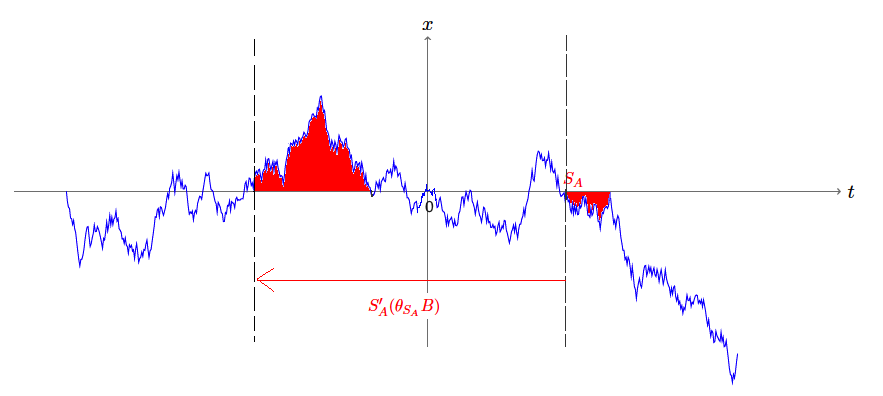
Figure 2: The times $S_{A}$ and $S_{A}^{{}^{\prime}}(\theta_{S_{A}}B)$ in a two-sided Brownian motion.

It is readily checked that there is a.s. a first excursion to the right of the origin with property $A$ and that this excursion is an $A$-excursion. But it is not an extra $A$-excursion. Indeed, the Brownian motion $B$ splits a.s. into a two-sided sequence of independent segments such that: every odd-numbered segment is an $A$-excursion; every even-numbered segment except the one enumerated $0$ is a standard Brownian motion starting from zero running until the first time that an $A$-excursion occurs; but the segment enumerated $0$ consists of two independent segments of that type. In addition to this, the origin of $B$ is placed at random in the segment enumerated $0$ according to the local time at zero of the segment. More details on this picture are given in Sections 5 and 6; see in particular Figure 2, Remark 6.3 and Remark 6.5.

In order to find an extra $A$-excursion we need to extend the general allocation (transport) theory for random measures that grew out of Liggett’s original paper. The shift described in the first paragraph, when applied to all the tails, generates an allocation from tails to heads; the allocation is balancing because it transports the counting measure for tails (source) into the counting measure for heads (target). In the recent papers [9, 15] and [18], balancing allocations for diffuse random measures on the line were used for unbiased Skorohod embedding and for unbiased embedding (by a random space-time shift) of the Brownian bridge. In this paper we shall allow the target measure to be non-diffuse. This is needed because the target measure associated with the $A$-excursions is a point process.

Before proceeding further, we need some notation. Let $\xi$ and $\eta$ be two jointly stationary and ergodic random measures on ${\mathbb{R}}$ with finite intensities $\lambda_{\xi}:=\mathbb{E}\xi[0,1]$ and $\lambda_{\eta}:=\mathbb{E}\eta[0,1]$. An allocation is a random (jointly measurable) mapping $t\mapsto\tau(t)$ from ${\mathbb{R}}$ to ${\mathbb{R}}\cup\{\infty\}$ which is equivariant under joint shifts of $t$ and the underlying randomness; see (2.3) for an exact definition. An allocation is said to balance the source  $\xi$  and the  target $\eta$ if $\mathbb{P}(\xi(\{s\in{\mathbb{R}}:\tau(s)=\infty\})>0)=0$ and the image measure of $\xi$ under $\tau$ is $\eta$; that is,

$$\int{\bf 1}\{\tau(s)\in C\}\,\xi(ds)=\eta(C),\quad C\in{\mathcal{B}}(\mathbb{R}),\,\mathbb{P}\text{-a.e.}$$ (1.1)

The balancing property (1.1) implies easily that

$$\lambda_{\xi}=\lambda_{\eta}.$$ (1.2)

The random variable $\tau(0)$ can be used to construct a shift-coupling (see [1, 20, 21]) of the Palm versions of $\xi$ and $\eta$; see [13, 4, 10].

In this paper, we prove that if the source $\xi$ is diffuse, and if the source and the target are mutually singular, then the equality (1.2) is not only necessary but also sufficient for the existence of a balancing allocation.

Theorem 1.1.

Assume that $\xi$ and $\eta$ are mutually singular jointly stationary and ergodic random measures on ${\mathbb{R}}$ such that $\xi$ is diffuse and $\lambda_{\xi}=\lambda_{\eta}$. Then the allocation $\tau$ defined by

$$\tau(s):=\inf\{t>s\colon\xi[s,t]\leq\eta[s,t]\},\quad s\in{\mathbb{R}},$$ (1.3)

balances $\xi$ and $\eta$.

In order to establish Theorem 1.1, we prove an even more general result, Theorem 3.2, which does not require $\xi$ to be diffuse; we construct a balancing transport kernel, provided that $\lambda_{\xi}=\lambda_{\eta}$ and that $\xi$ and $\eta$ are mutually singular. This relies heavily on Theorem 5.1 from [9], a precursor of Theorem 1.1 where both $\xi$ and $\eta$ are assumed to be diffuse.

Transports of random measures and point processes have been studied on more general phase spaces. For further background we refer to [20, 12, 3, 4, 10, 9, 5]. The existence of an extra head was implicit in an abstract group result in [20], but in that paper there was no hint at an explicit pathwise method of finding an extra head. In [12, 3], the sources are counting and Lebesgue measures and the targets are Bernoulli and Poisson processes. In [4], the source is Lebesgue measure and the target is a simple point process, in particular a Poisson process. In [9], the source and target are both diffuse random measures on the line, in particular local times of Brownian motion. In Theorem 1.1 above, the source is diffuse but the target is general, and according to Theorem 3.2 below (see Remark 4.2), a balancing allocation is obtained through external randomization in the case where both source and target are general. The paper [10] develops a general transport theory for random measures (on Abelian groups) with focus on transport kernels rather than only allocations. The allocations studied in the present paper have a certain property of right-stability; see [9, Section 7]. The mass of the source prefers to be allocated as close as possible. The paper [5] pursues a different approach, based on the minimization of expected transport costs (defined in the Palm sense). It is shown that if the expected transport cost is finite and the source is absolutely continuous, then there exists a unique optimal allocation that can be locally approximated with solutions to the classical Monge problem (see [22]).

The paper is organised as follows. Section 2 gives preliminaries on random measures, transport kernels and allocations. Section 3 provides the main transport result, Theorem 3.2. We then turn to the application to Brownian motion. Section 4 contains the key Palm and shift-coupling result for the embedding, Proposition 4.1. Section 5 is devoted to excursion theory and discusses the embedding problem. Section 6 applies Proposition 4.1 to unbiased embedding of conditional Itô measures. We also apply this proposition to Bismut’s excursion measure, a close relative of Itô’s measure.

2 Preliminaries

Let $(\Omega,\mathcal{F},\mathbb{P})$ be a $\sigma$-finite measure space with associated integral operator $\mathbb{E}$. A random measure (resp. point process) $\xi$ on ${\mathbb{R}}$ (equipped with its Borel $\sigma$-field ${\mathcal{B}}({\mathbb{R}})$) is a kernel from $\Omega$ to ${\mathbb{R}}$ such that $\xi(\omega,C)<\infty$ (resp. $\xi(\omega,C)\in{\mathbb{N}}_{0}$) for $\mathbb{P}$-a.e. $\omega$ and all compact $C\subset{\mathbb{R}}$. We assume that $(\Omega,\mathcal{F})$ is equipped with a measurable flow $\theta_{s}\colon\Omega\to\Omega$, $s\in{\mathbb{R}}$. This is a family of mappings such that $(\omega,s)\mapsto\theta_{s}\omega$ is measurable, $\theta_{0}$ is the identity on $\Omega$ and

$$\theta_{s}\circ\theta_{t}=\theta_{s+t},\quad s,t\in{\mathbb{R}},$$ (2.1)

where $\circ$ denotes composition.

A kernel $\xi$ from $\Omega$ to ${\mathbb{R}}$ is said to be invariant (or flow-adapted) if

$$\xi(\theta_{t}\omega,C-t)=\xi(\omega,C),\quad C\in\mathcal{B}(\mathbb{R}),t\in{\mathbb{R}},\mathbb{P}\text{-a.e.\ $\omega\in\Omega$}.$$ (2.2)

We assume that the measure $\mathbb{P}$ is stationary; that is

$$\mathbb{P}\circ\theta_{s}=\mathbb{P},\quad s\in{\mathbb{R}},$$

where $\theta_{s}$ is interpreted as a mapping from $\mathcal{F}$ to $\mathcal{F}$ in the usual way:

$$\theta_{s}A:=\{\theta_{s}\omega:\omega\in A\},\quad A\in\mathcal{F},\,s\in{\mathbb{R}}.$$

The invariant $\sigma$-field $\mathcal{I}\subset\mathcal{F}$ is the class of all sets $A\in\mathcal{F}$ satisfying $\theta_{s}A=A$ for all $s\in{\mathbb{R}}$. We also assume that $\mathbb{P}$ is ergodic; that is for any $A\in\mathcal{I}$, we have either $\mathbb{P}(A)=0$ or $\mathbb{P}(A^{c})=0$.

Remark 2.1.

The assumption of ergodicity has been made for simplicity and can be relaxed. The assumption $\lambda_{\xi}=\lambda_{\eta}$ has then to be replaced by

$$\mathbb{E}[\xi[0,1]\mid\mathcal{I}]=\mathbb{E}[\eta[0,1]\mid\mathcal{I}],\quad\mathbb{P}\text{-a.e.}$$

We refer to [10] for more detail on this point.

A transport kernel is a sub-Markovian kernel $K$ from $\Omega\times{\mathbb{R}}$ to ${\mathbb{R}}$. A transport kernel is invariant if

$$K(\theta_{s}\omega,0,C-s)=K(\omega,s,C),\quad\quad s\in{\mathbb{R}},\,C\in{\mathcal{B}}({\mathbb{R}}),\,\text{$\mathbb{P}$-a.e.\ $\omega\in\Omega$}.$$

An allocation [4, 10] is a measurable mapping $\tau\colon\Omega\times{\mathbb{R}}\rightarrow{\mathbb{R}}\cup\{\infty\}$ that is equivariant in the sense that

$$\tau(\theta_{t}\omega,s-t)=\tau(\omega,s)-t,\quad s,t\in{\mathbb{R}},\,\text{$\mathbb{P}$-a.e.\ $\omega\in\Omega$}.$$ (2.3)

Any allocation defines a transport kernel $K$ by $K(s,\cdot)={\bf 1}\{\tau(s)<\infty\}\delta_{\tau(s)}$.

Remark 2.2.

In [10], a transport kernel $K$ is Markovian; that is $K(\omega,s,{\mathbb{R}})=1$ for all $s\in{\mathbb{R}}$. We find it convenient to allow for $K(\omega,s,{\mathbb{R}})<1$ on an exceptional set of points $(\omega,s)$. In the same spirit, we do not assume an allocation to take on only finite values, as it is the case in [10, 9].

Let $\xi$ and $\eta$ be random measures on ${\mathbb{R}}$. We say that a transport kernel $K$ balances $\xi$ and $\eta$ if $K(\omega,s,{\mathbb{R}})=1$ a.e. w.r.t. the measure $\xi(\omega,ds)\mathbb{P}(d\omega)$ and $K$ transports $\xi$ to $\eta$, that is,

$$\int K(s,\cdot)\,\xi(ds)=\eta,\quad\mathbb{P}\text{-a.e.}$$ (2.4)

If $\tau$ is an allocation such that the associated transport kernel $K$ balances $\xi$ and $\eta$, then we say that $\tau$ balances $\xi$ and $\eta$.

3 Balancing mutually singular random measures

Throughout this section, let $\xi$ and $\eta$ be two invariant random measures defined on the $\sigma$-finite measure space $(\Omega,\mathcal{F},\mathbb{P})$. We recall from the previous section that $\mathbb{P}$ is assumed to be stationary and ergodic under a given flow. In particular, the joint distribution of $\xi$ and $\eta$ is stationary and ergodic. We shall construct a transport kernel balancing $\xi$ and $\eta$. To this end, we use the following result from [9, Theorem 5.1] in a crucial way.

Theorem 3.1.

Assume that $\xi$ and $\eta$ are mutually singular diffuse invariant random measures such that $\lambda_{\xi}=\lambda_{\eta}$. Then the mapping $\tau$ defined by (1.3) is an allocation balancing $\xi$ and $\eta$.

For any $u\in[0,1]$ we define a mapping $\tau^{u}\colon\Omega\times{\mathbb{R}}\rightarrow[0,\infty]$ by

$$\tau^{u}(s):=\inf\{t>s\colon u\xi\{s\}+\xi(s,t)\leq\eta[s,t]\},\quad s\in{\mathbb{R}},$$ (3.1)

where $\inf\emptyset:=\infty$.

Theorem 3.2.

Assume that $\xi$ and $\eta$ are mutually singular invariant random measures on ${\mathbb{R}}$ such that $\lambda_{\xi}=\lambda_{\eta}$. Then

$$K(s,C):=\int^{1}_{0}{\bf 1}\{\tau^{u}(s)\in C\}\,du,\quad s\in{\mathbb{R}},\,C\in{\mathcal{B}}({\mathbb{R}}),$$ (3.2)

defines a transport kernel balancing $\xi$ and $\eta$.

Since $\xi$ and $\eta$ are invariant, we obtain for all $\omega$ outside a $\mathbb{P}$-null set, for all $s,t\in{\mathbb{R}}$ and for all $u\in[0,1]$ that

$$\tau^{u}(\theta_{t}\omega,s-t) =\inf\{r>s-t\colon u\xi(\theta_{t}\omega,\{s-t\})+\xi(\theta_{t}\omega,(s-t,r))\leq\eta(\theta_{t}\omega,[s-t,r])\}$$

$$=\inf\{r>s-t\colon u\xi(\omega,\{s\})+\xi(\omega,(s,r+t))\leq\eta(\omega,[s,r+t])\}$$

$$=\tau^{u}(\omega,s)-t.$$

Hence $\tau^{u}$ is an allocation and (3.2) defines a transport kernel.

If $s\in{\mathbb{R}}$ satisfies $\xi\{s\}=0$, then $\tau^{u}(s)=\tau^{0}(s)$ does not depend on $u\in[0,1]$. Therefore the kernel (3.2) reduces on $\{s:\xi\{s\}=0\}$ to the allocation rule $\tau^{0}$, that is

$$K(s,\cdot)={\bf 1}\{\xi\{s\}=0\}\delta_{\tau^{0}(s)}+{\bf 1}\{\xi\{s\}>0\}\int^{1}_{0}{\bf 1}\{\tau^{u}(s)\in\cdot\}\,du.$$ (3.3)

If $\xi\{s\}>0$, then we may think of $u\xi\{s\}$ as a location picked at random in the mass of $\xi$ at $s$, before applying virtually the same rule $\tau$ as in Theorem 3.1. If $\xi$ is diffuse, then $\tau^{0}=\tau$, where $\tau$ is given by (1.3). Moreover, the second term on the r.h.s. of (3.3) vanishes in this case. Thus, Theorem 3.2 implies Theorem 1.1.

Remark 3.3.

Theorem 1.1 is wrong without the assumption of mutual singularity. To see this, let $\xi^{\prime}$ and $\eta^{\prime}$ be mutually singular invariant random measures on ${\mathbb{R}}$ such that $\lambda_{\xi^{\prime}}=\lambda_{\eta^{\prime}}<\infty$. Assume that $\xi^{\prime}$ is diffuse. Let $\xi:=\xi^{\prime}+\mu_{1}$ and $\eta:=\eta^{\prime}+\mu_{1}$, where $\mu_{1}$ is Lebesgue measure on ${\mathbb{R}}$. Then the allocation (1.3) takes the form

$$\tau(s):=\inf\{t>s\colon\xi^{\prime}[s,t]\leq\eta^{\prime}[s,t]\},\quad s\in{\mathbb{R}}.$$

By Theorem 1.1, $\tau$ balances $\xi^{\prime}$ and $\eta^{\prime}$. Therefore, $\tau$ balances $\xi$ and $\eta$ iff

$$\int{\bf 1}\{\tau(s)\in\cdot\}\,\mu_{1}(ds)=\mu_{1},\quad\mathbb{P}\text{-a.e.}$$ (3.4)

This cannot be true in general. For a simple example let $\xi_{0}$ be Lebesgue measure on the set $A:=\cup_{i\in 3{\mathbb{Z}}}[i,i+2)$ and let $\eta_{0}$ be twice the Lebesgue measure on the set ${\mathbb{R}}\setminus A$. Assume that $(\xi^{\prime},\eta^{\prime})=(\theta_{U}\xi_{0},\theta_{U}\eta_{0})$, where $U$ is uniformly distributed on the interval $[0,3)$ and where we abuse notation by introducing for any measure $\mu$ on ${\mathbb{R}}$ and $s\in{\mathbb{R}}$ a new measure $\theta_{s}\mu$ by $\theta_{s}\mu:=\mu(\cdot+s)$. For $s\in[U,U+2)$ we then have $\tau(s)=3U/2+3-s/2$, so that $\int^{U+2}_{U}{\bf 1}\{\tau(s)\in\cdot\}\,\mu_{1}(ds)$ is twice the Lebesgue measure on $[U+2,U+3)$. Hence (3.4) fails. Note that (3.4) fails, even when modifying $\tau$ on the support of $\eta^{\prime}$ in an arbitrary manner.

The proof of Theorem 3.2 relies on Theorem 3.1 and the six lemmas below. Of these lemmas all are deterministic except the final one, Lemma 3.9. For convenience we assume that $\xi$ and $\eta$ are locally finite everywhere on $\Omega$. We shall use the decomposition $\xi=\xi^{c}+\xi^{d}$ of $\xi$ as the sum of its diffuse part $\xi^{c}$ and its purely discrete part $\xi^{d}$. The formulas $\xi^{c}(dt):={\bf 1}\{\xi\{t\}=0\}\xi(dt)$ and $\xi^{d}(dt):={\bf 1}\{\xi\{t\}>0\}\xi(dt)$ show that these random measures are again invariant. Similar definitions apply to $\eta$.

Theorem 3.1 assumes $\xi$ and $\eta$ to be diffuse (and mutually singular). In order to obtain a diffuse source and target, we introduce a time change, by stretching the real axis at the position of an atom by its size. For that purpose we define, for $s\in{\mathbb{R}}$,

$$\zeta(s):=\begin{cases}s+\xi^{d}[0,s)+\eta^{d}[0,s),\quad&s\geq 0,\\ s-\xi^{d}[s,0)-\eta^{d}[s,0),\quad&s<0.\end{cases}$$

Define a random measure $\xi^{*}$ on ${\mathbb{R}}$ by

$$\xi^{*}(C):=\int{\bf 1}\{\zeta(t)\in C\}\,\xi^{c}(dt)+\iint{\bf 1}\{\zeta(t)\leq v\leq\zeta(t)+\xi\{t\},v\in C\}\xi\{t\}^{-1}\,dv\,\xi^{d}(dt).$$

Define another random measure $\eta^{*}$ on ${\mathbb{R}}$ by replacing $\xi$ with $\eta$ in the above r.h.s. Then $\xi^{*}$ and $\eta^{*}$ are diffuse, and it is easy to check that these random measures are again mutually singular.

To express $(\xi,\eta)$ in terms of $(\xi^{*},\eta^{*})$, we use the generalized inverse $\zeta^{-1}$ of $\zeta$, defined by

$$\zeta^{-1}(t):=\inf\{s\in{\mathbb{R}}\colon\zeta(s)\geq t\},\quad t\in{\mathbb{R}}.$$

Since $\zeta$ is strictly increasing, the inverse time change $\zeta^{-1}$ is continuous.

Lemma 3.4.

Let $s\in{\mathbb{R}}$ and $v\in[0,\xi\{s\}\vee\eta\{s\}]$. Then $\zeta^{-1}(\zeta(s)+v)=s$.

Proof.

Since $\zeta$ is (strictly) increasing, it is easy to prove the equivalence

$$\zeta(s)\leq t\;\Longleftrightarrow\;s\leq\zeta^{-1}(t),$$ (3.5)

valid for all $s,t\in{\mathbb{R}}$. Applying this to the trivial inequality $\zeta(s)\leq\zeta(s)+v$ yields $s\leq\zeta^{-1}(\zeta(s)+v)$. Assume by contradiction that this inequality is strict, that is, $s<s^{\prime}$ where $s^{\prime}=\zeta^{-1}(\zeta(s)+v)$. Trivially, $s^{\prime}\leq\zeta^{-1}(\zeta(s)+v)$ and (3.5) yields $\zeta(s^{\prime})\leq\zeta(s)+v$. This, together with $v\leq\xi\{s\}\vee\eta\{s\}$, implies (for $s\geq 0$; the case $s<0$ is similar) that

$$s^{\prime}+\xi^{d}[0,s^{\prime})+\eta^{d}[0,s^{\prime})\leq s+\xi^{d}[0,s]+\eta^{d}[0,s].$$

Now $s^{\prime}>s$ and $\xi^{d}[0,s^{\prime})+\eta^{d}[0,s^{\prime})\geq\xi^{d}[0,s]+\eta^{d}[0,s]$, which leads to a contradiction. ∎

Lemma 3.5.

Let $s_{1}<s_{2}$, $v_{1}\in[0,\xi\{s_{1}\}\vee\eta\{s_{1}\}]$ and $v_{2}\in[0,\xi\{s_{2}\}\vee\eta\{s_{2}\}]$. Then

$$\xi^{*}[\zeta(s_{1})+v_{1},\zeta(s_{2})+v_{2}]={\bf 1}\{\eta\{s_{1}\}=0\}(\xi\{s_{1}\}-v_{1})+\xi(s_{1},s_{2})+{\bf 1}\{\eta\{s_{2}\}=0\}v_{2}.$$

Proof.

Since $\xi^{*}$ is diffuse, we have

$$\xi^{*}[\zeta(s_{1})+v_{1},\zeta(s_{2})+v_{2}]=\int{\bf 1}\{\zeta(s_{1})+v_{1}<t\leq\zeta(s_{2})+v_{2}\}\,\xi^{*}(dt)=I_{1}+I_{2},$$

where

$$I_{1} :=\int{\bf 1}\{\zeta(s_{1})+v_{1}<\zeta(s)\leq\zeta(s_{2})+v_{2}\}\,\xi^{c}(ds),$$

$$I_{2} :=\sum_{s\in{\mathbb{R}}}{\bf 1}\{\xi\{s\}>0\}\int{\bf 1}\{\zeta(s)<v\leq\zeta(s)+\xi\{s\},\zeta(s_{1})+v_{1}<v\leq\zeta(s_{2})+v_{2}\}\,dv.$$

Apply first (3.5) and then Lemma 3.4 to obtain

$$I_{1}=\int{\bf 1}\{s_{1}<s\leq s_{2}\}\,\xi^{c}(ds)=\xi^{c}(s_{1},s_{2}).$$ (3.6)

Turning to $I_{2}$, we restrict ourselves to the case $\eta\{s_{1}\}=\eta\{s_{2}\}=0$. The other cases can be treated similarly. First note that the inequalities $v\leq\zeta(s)+\xi\{s\}$ and $\zeta(s_{1})+v_{1}\leq v$ imply $s_{1}\leq s$ (by Lemma 3.4), while the inequalities $v\leq\zeta(s_{2})+v_{2}$ and $\zeta(s)\leq v$ imply $s\leq s_{2}$. Splitting into the three cases  $s=s_{1}$,  $s_{1}<s<s_{2}$,  $s=s_{2}$  yields

$$I_{2}= {\bf 1}\{\xi\{s_{1}\}>0\}\int{\bf 1}\{\zeta(s_{1})+v_{1}<v\leq\zeta(s_{1})+\xi\{s_{1}\}\}\,dv$$

$$+\sum_{s_{1}<s<s_{2}}{\bf 1}\{\xi\{s\}>0\}\int{\bf 1}\{\zeta(s)<v\leq\zeta(s)+\xi\{s\}\}\,dv$$

$$+{\bf 1}\{\xi\{s_{2}\}>0\}\int{\bf 1}\{\zeta(s_{2})<v\leq\zeta(s_{2})+v_{2}\}\,dv.$$

It follows that

$$I_{2}=\xi\{s_{1}\}-v_{1}+\xi^{d}(s_{1},s_{2})+v_{2}.$$

Combining this with (3.6) yields the assertion of the lemma. ∎

According to the following change-of-variable result, $\zeta^{-1}$ balances $\xi^{*}$ and $\xi$.

Lemma 3.6.

Let $f\colon{\mathbb{R}}\to[0,\infty)$ be measurable. Then

$$\int f(s)\,\xi(ds)=\int f(\zeta^{-1}(t))\,\xi^{*}(dt).$$ (3.7)

Proof.

It suffices to establish (3.7) for $f:={\bf 1}_{[a,b)}$, where $a<b$. Using (3.5) we obtain

$$\int{\bf 1}_{[a,b)}(\zeta^{-1}(t))\,\xi^{*}(dt)=\int{\bf 1}\{\zeta(a)\leq t<\zeta(b)\}\,\xi^{*}(dt)=\xi[a,b),$$

where we have used Lemma 3.5 (with $v_{1}=v_{2}=0$) to get the second identity. ∎

Define

$$\tau^{*}(s):=\inf\{t>s\colon\xi^{*}[s,t]\leq\eta^{*}[s,t]\},\quad s\in{\mathbb{R}}.$$ (3.8)

Lemma 3.7.

Let $s\in{\mathbb{R}}$ with $\xi\{s\}=\eta\{s\}=0$. Then $\tau^{*}(\zeta(s))<\infty$ iff $\tau^{0}(s)<\infty$. In this case

$$\zeta^{-1}(\tau^{*}(\zeta(s)))=\tau^{0}(s).$$ (3.9)

Proof.

We abbreviate $t^{*}:=\tau^{*}(\zeta(s))$.

First consider the case $t^{*}=\zeta(s)$. Then $\zeta^{-1}(t^{*})=s$ (by Lemma 3.4) and we need to show that $\tau^{0}(s)=s$. There are $t_{n}>t^{*}$, $n\in{\mathbb{N}}$, such that $\xi^{*}[\zeta(s),t_{n}]\leq\eta^{*}[\zeta(s),t_{n}]$ and $t_{n}\downarrow t^{*}$. We distinguish two cases. In the first case, there are infinitely many $n\in{\mathbb{N}}$ such that $t_{n}=\zeta(s_{n})+v_{n}$ for some $s_{n}\in{\mathbb{R}}$ satisfying $\eta\{s_{n}\}=0$ and $v_{n}\in[0,\xi\{s_{n}\}]$. Lemma 3.5 implies $\xi[s,s_{n})+v_{n}\leq\eta[s,s_{n}]$ and hence $\xi[s,s_{n})\leq\eta[s,s_{n}]$. Since $t^{*}<t_{n}=\zeta(s_{n}+v_{n})$ we obtain from (3.5) and Lemma 3.4 that $s_{n}>\zeta^{-1}(t^{*})=s$. Lemma 3.4 and the continuity of $\zeta^{-1}$ imply $s_{n}=\zeta^{-1}(t_{n})\downarrow\zeta^{-1}(t^{*})=s$ along the chosen subsequence. Hence $\tau^{0}(s)=s$. In the second case, there are infinitely many $n\in{\mathbb{N}}$ such that $t_{n}=\zeta(s_{n})+v_{n}$ for some $s_{n}\in{\mathbb{R}}$ satisfying $\eta\{s_{n}\}>0$ and $v_{n}\in[0,\eta\{s_{n}\}]$. Then $\xi\{s_{n}\}=0$ and Lemma 3.5 implies $\xi[s,s_{n})\leq\eta[s,s_{n})+v_{n}$ and hence $\xi[s,s_{n})\leq\eta[s,s_{n}]$. As before, it follows that $s_{n}>s$ and $s_{n}\downarrow s$ along the chosen subsequence. Hence $\tau^{0}(s)=s$ in this case.

Assume next that $t^{*}\in(\zeta(s),\infty)$. By definition,

$$\xi^{*}[\zeta(s),r]>\eta^{*}[\zeta(s),r],\quad\zeta(s)<r<t^{*},$$ (3.10)

as well as

$$\xi^{*}[\zeta(s),t^{*}]=\eta^{*}[\zeta(s),t^{*}].$$ (3.11)

Assume first that $t^{*}=\zeta(t)+v$ for some $t\geq s$ with $\eta\{t\}=0$ and $v\in[0,\xi\{t\}]$. Then $t>s$ (by (3.11)) and Lemma 3.4 implies that $\zeta^{-1}(t^{*})=t$. We want to show that $\tau^{0}(s)=t$. Let $t^{\prime}\in(s,t)$. If $\xi\{t^{\prime}\}=0$, we set $r:=\zeta(t^{\prime})+\eta\{t^{\prime}\}$. Then $r<\zeta(t)\leq t^{*}$ and (3.10) together with Lemma 3.5 imply that $\xi[s,t^{\prime})>\eta[s,t^{\prime}]$. If $\xi\{t^{\prime}\}>0$, we set $r:=\zeta(t^{\prime})$ to obtain the same inequality and hence

$$\xi[s,t^{\prime})>\eta[s,t^{\prime}],\quad s<t^{\prime}<t.$$ (3.12)

On the other hand, we have from (3.11) and Lemma 3.5 that $\xi[s,t)+v=\eta[s,t]$, so that $\xi[s,t)\leq\eta[s,t]$. Hence $\tau^{0}(s)=t=\zeta^{-1}(t^{*})$ and (3.9) follows.

The second possible case is $t^{*}=\zeta(t)+v$ for some $t\geq s$ with $\eta\{t\}>0$ and $v\in[0,\eta\{t\}]$. Since $\xi$ and $\eta$ are mutually singular, we have $\xi\{t\}=0$. Again this implies $t>s$ and (3.12). Lemma 3.5 implies that $\xi[s,t)+v=\eta[s,t)$ and hence $\xi[s,t)\leq\eta[s,t]$. Therefore $\tau^{0}(s)=t=\zeta^{-1}(t^{*})$, where we have used Lemma 3.4.

Assume, finally, that $t^{*}=\infty$, so that (3.10) holds for all $r>\zeta(s)$. Let $t^{\prime}>s$. If $\xi\{t^{\prime}\}=\eta\{t^{\prime}\}=0$, we take $r=\zeta(t^{\prime})$ to obtain from Lemma 3.5 that $\xi[s,t^{\prime})>\eta[s,t^{\prime}]$. If $\xi\{t^{\prime}\}>0$ (and hence $\eta\{t^{\prime}\}=0$), we take $r=\zeta(t^{\prime})$ to obtain from Lemma 3.5 that $\xi[s,t^{\prime})>\eta[s,t^{\prime}]$. If $\eta\{t^{\prime}\}>0$ (and hence $\xi\{t^{\prime}\}=0$), we take $r=\zeta(t^{\prime})+\eta\{t^{\prime}\}$ to obtain from Lemma 3.5 that $\xi[s,t^{\prime})>\eta[s,t^{\prime}]$. Hence $\tau^{0}(s)=\infty$. ∎

Lemma 3.8.

Let $s\in{\mathbb{R}}$ with $\xi\{s\}>0$ and $u\in[0,1)$. Then $\tau^{*}(\zeta(s)+u\xi\{s\})<\infty$ iff $\tau^{1-u}(s)<\infty$. In this case

$$\zeta^{-1}(\tau^{*}(\zeta(s)+u\xi\{s\}))=\tau^{1-u}(s).$$ (3.13)

Proof.

Since $\xi$ and $\eta$ are mutually singular we have $\eta\{s\}=0$. Moreover, since $u<1$ we have $\eta[s,s+\varepsilon]<(1-u)\xi\{s\}$ for all sufficiently small $\varepsilon>0$ and therefore $\tau^{1-u}(s)>s$ and (by Lemma 3.5) $\tau^{*}(\zeta(s)+u\xi\{s\})>\zeta(s)$. The proof can now proceed similar to that of Lemma 3.7. The main tool is again Lemma 3.5. In contrast to the case $\xi\{s\}=0$, it has to be applied with $s_{1}=s$ and $v_{1}=u\xi\{s\}$. Further details are omitted. ∎

In the upcoming proof of Theorem 3.2, we will use that $\tau^{*}$ balances $\xi^{*}$ and $\eta^{*}$. Since $\xi^{*}$ and $\eta^{*}$ need not be jointly stationary, Theorem 3.1 cannot be used directly to establish this fact. As an intermediate step, we need the following lemma which presents (shifted and length-biased) versions of $\xi^{*}$ and $\eta^{*}$ that Theorem 3.1 can be applied to. As before we abuse notation by introducing for any measure $\mu$ on ${\mathbb{R}}$ and $s\in{\mathbb{R}}$ a new measure $\theta_{s}\mu$ by $\theta_{s}\mu:=\mu(\cdot+s)$. If $\mu^{\prime}$ is another measure on ${\mathbb{R}}$, we write $\theta_{s}(\mu,\mu^{\prime}):=(\theta_{s}\mu,\theta_{s}\mu^{\prime})$.

Lemma 3.9.

Let $\xi$ and $\eta$ be random measures on ${\mathbb{R}}$ defined on $(\Omega,\mathcal{F},\mathbb{P})$ and let $\xi^{*}$ and $\eta^{*}$ be as above. Extend $(\Omega,\mathcal{F},\mathbb{P})$ so as to support a random variable $U$ that is uniform on $[0,1)$ conditionally on $(\xi^{*},\eta^{*})$. Let $S_{1}=1+\xi^{d}[0,1)+\eta^{d}[0,1)$ and define a $\sigma$-finite measure $\mathbb{P}^{*}$ on $(\Omega,\mathcal{F})$ by $d\mathbb{P}^{*}=S_{1}d\mathbb{P}$. Then the distribution of $\theta_{US_{1}}(\xi^{*},\eta^{*})$ is stationary and ergodic under $\mathbb{P}^{*}$ and the intensities are

$$\mathbb{E}^{*}(\theta_{US_{1}}\xi^{*})[0,1)=\mathbb{E}\xi[0,1),\quad\mathbb{E}^{*}(\theta_{US_{1}}\eta^{*})[0,1)=\mathbb{E}\eta[0,1).$$

Proof.

Let $M$ denote the space of locally finite measures on ${\mathbb{R}}$, equipped with the natural Kolmogorov $\sigma$-field. We have assumed that $\xi$ and $\eta$ are random elements of $M$.

Take $t\geq 0$ and let $f\colon M\times M\to[0,\infty)$ be bounded and measurable. For $n\in\mathbb{N}$, let $A_{n}\in\mathcal{F}$ be such that $\mathbb{P}(A_{n})<\infty$ and $A_{1}\subset A_{2}\subset A_{3}\subset\dots\uparrow\Omega$. Set $f_{n}=f1_{A_{n}}$ and note that $\mathbb{P}(A_{n})<\infty$ implies that $\mathbb{E}\int_{S_{1}}^{S_{1}+t}f_{n}(\theta_{s}(\xi^{*},\eta^{*}))ds$ is finite. Since $\int_{t}^{S_{1}}f_{n}(\theta_{s}(\xi^{*},\eta^{*}))ds$ could be negative, the finiteness is needed for the last equality in

$$\mathbb{E}^{*}f_{n}(\theta_{t}\theta_{US_{1}}(\xi^{*},\eta^{*})) =\mathbb{E}S_{1}f_{n}(\theta_{t}\theta_{US_{1}}(\xi^{*},\eta^{*}))=\mathbb{E}\int_{t}^{S_{1}+t}f_{n}(\theta_{s}(\xi^{*},\eta^{*}))ds$$

$$=\mathbb{E}\int_{t}^{S_{1}}f_{n}(\theta_{s}(\xi^{*},\eta^{*}))ds+\mathbb{E}\int_{S_{1}}^{S_{1}+t}f_{n}(\theta_{s}(\xi^{*},\eta^{*}))ds.$$

Now note that $\theta_{S_{1}}(\xi^{*},\eta^{*})$ is the same measurable mapping of $\theta_{1}(\xi,\eta)$ as $(\xi^{*},\eta^{*})$ is of $(\xi,\eta)$. Since $\theta_{1}(\xi,\eta)$ has the same $\mathbb{P}$-distribution as $(\xi,\eta)$, this implies that $\theta_{S_{1}}(\xi^{*},\eta^{*})$ has the same $\mathbb{P}$-distribution as $(\xi^{*},\eta^{*})$. This further yields the first equality in

$$\mathbb{E}^{*}f_{n}(\theta_{t}\theta_{US_{1}}(\xi^{*},\eta^{*})) =\mathbb{E}\int_{t}^{S_{1}}f_{n}(\theta_{s}(\xi^{*},\eta^{*}))ds+\mathbb{E}\int_{0}^{t}f_{n}(\theta_{s}(\xi^{*},\eta^{*}))ds$$

$$=\mathbb{E}\int_{0}^{S_{1}}f_{n}(\theta_{s}(\xi^{*},\eta^{*}))ds.$$

Send $n\to\infty$ and use the monotone convergence theorem to obtain

$$\mathbb{E}^{*}f(\theta_{t}\theta_{US_{1}}(\xi^{*},\eta^{*}))=\mathbb{E}\int_{0}^{S_{1}}f(\theta_{s}(\xi^{*},\eta^{*}))ds.$$

So $\mathbb{E}^{*}f(\theta_{t}\theta_{US_{1}}(\xi^{*},\eta^{*}))$ does not depend on $t$; that is, $\theta_{US_{1}}(\xi^{*},\eta^{*})$ is stationary under $\mathbb{P}^{*}$.

Next we prove the ergodicity assertion. It is not hard to prove that

$$((\theta_{t}\xi)^{*},(\theta_{t}\eta)^{*})=(\theta_{\zeta(t)}\xi^{*},\theta_{\zeta(t)}\eta^{*}),\quad t\in{\mathbb{R}}.$$ (3.14)

Let $A\subset M\times M$ be a measurable set that is invariant under diagonal shifts. Then (3.14) shows for all $(\omega,t)\in\Omega\times{\mathbb{R}}$ that $(\xi(\theta_{t}\omega)^{*},\eta(\theta_{t}\omega)^{*})\in A$ if and only if $(\xi(\omega)^{*},\eta(\omega)^{*})\in A$. Since $\mathbb{P}$ is ergodic, we obtain that either $\mathbb{P}((\xi^{*},\eta^{*})\in A)=0$ or $\mathbb{P}((\xi^{*},\eta^{*})\notin A)=0$. Therefore, the ergodicity of the shifted length-biased version of $(\xi^{*},\eta^{*})$ follows from the two facts that the zero sets of $\mathbb{P}^{*}$ are the same as those of $\mathbb{P}$, and that randomly shifted invariant sets remain invariant.

It remains to prove the intensity result. Let $\mu_{1}$ be Lebesgue measure on ${\mathbb{R}}$. Since $\mu_{1}$ is shift-invariant and $\theta_{S_{1}}\xi^{*}$ has the same $\mathbb{P}$-distribution as $\xi^{*}$, we have

$$\mathbb{E}(\mu_{1}\otimes\xi^{*})(A)=\mathbb{E}(\mu_{1}\otimes\xi^{*})((S_{1},S_{1})+A),\quad A\in\mathcal{B}({\mathbb{R}}^{2}).$$

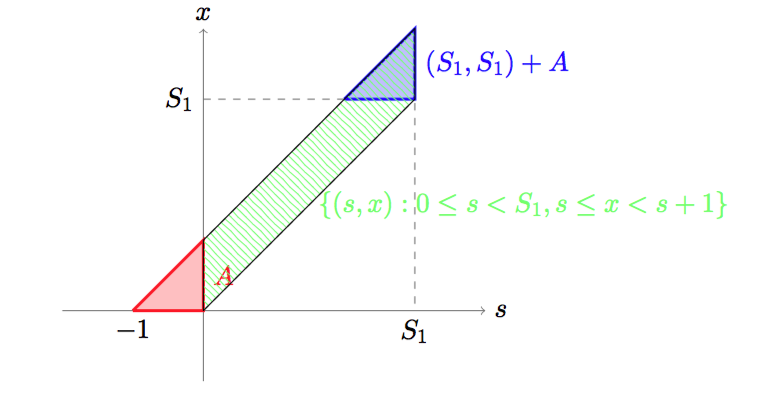
Figure 1: The region $\{(s,x):0\leq s<S_{1},s\leq x<s+1\}$ has the same Lebesgue measure as $(\{(s,x):0\leq x<S_{1},x-1<s\leq x\}\setminus A)\cup((S_{1},S_{1})+A)$.

Apply this with $A=\{(s,x):-1\leq s<0,0\leq x<s+1\}$ to obtain

$$\mathbb{E}^{*}( \theta_{US_{1}}\xi^{*})[0,1)=\mathbb{E}S_{1}\int_{0}^{1}(\theta_{uS_{1}}\xi^{*})[0,1)du=\mathbb{E}\int_{0}^{S_{1}}\xi^{*}(s+[0,1))ds$$

$$=\mathbb{E}(\mu_{1}\otimes\xi^{*})(\{(s,x):0\leq s<S_{1},s\leq x<s+1\})$$

$$=\mathbb{E}(\mu_{1}\otimes\xi^{*})((\{(s,x):0\leq x<S_{1},x-1<s\leq x\}\setminus A)\cup((S_{1},S_{1})+A))$$

$$=\mathbb{E}(\mu_{1}\otimes\xi^{*})(\{(s,x):0\leq x<S_{1},x-1<s\leq x\})$$

$$\qquad\qquad\qquad\qquad\qquad\qquad-\mathbb{E}(\mu_{1}\otimes\xi^{*})(A)+\mathbb{E}(\mu_{1}\otimes\xi^{*})((S_{1},S_{1})+A))$$

$$=\mathbb{E}(\mu_{1}\otimes\xi^{*})(\{(s,x):0\leq x<S_{1},x-1<s<x\})$$

$$=\mathbb{E}\xi^{*}[0,S_{1})=\mathbb{E}\xi[0,1).$$

In the same way, we obtain $\mathbb{E}^{*}(\theta_{US_{1}}\eta^{*})[0,1)=\mathbb{E}\eta[0,1)$. ∎

Proof of Theorem 3.2.

By Theorem 3.1 and Lemma 3.9, the random mapping $\tau^{\prime}\colon{\mathbb{R}}\to[0,\infty]$ defined by

$$\tau^{\prime}(s):=\inf\{t>s\colon(\theta_{US_{1}}\xi^{*})[s,t]\leq(\theta_{US_{1}}\eta^{*})[s,t]\},\quad s\in{\mathbb{R}},$$

balances $\theta_{US_{1}}\xi^{*}$ and $\theta_{US_{1}}\eta^{*}$ under $\mathbb{P}^{*}$. Since $\mathbb{P}^{*}$ and $\mathbb{P}$ are equivalent, this implies that $\tau^{\prime}$ balances $\theta_{US_{1}}\xi^{*}$ and $\theta_{US_{1}}\eta^{*}$ under $\mathbb{P}$. This remains true if the origin is shifted to some random location. Recall the definition (3.8) of $\tau^{*}$. Shift the origin to $-US_{1}$ to obtain

$$\tau^{*}=\tau^{\prime}(\cdot-US_{1})+US_{1},\qquad\xi^{*}=\theta_{-US_{1}}\theta_{US_{1}}\xi^{*},\qquad\eta^{*}=\theta_{-US_{1}}\theta_{US_{1}}\eta^{*}.$$

Thus, $\tau^{*}$ balances $\xi^{*}$ and $\eta^{*}$ under $\mathbb{P}$. We assume for simplicity that

$$\int{\bf 1}\{\tau^{*}(s)\in\cdot\}\,\xi^{*}(ds)=\eta^{*}$$ (3.15)

holds everywhere on $\Omega$.

We want to prove that

$$\iint f(t)\,K(s,dt)\,\xi(ds)=\int f(s)\,\eta(ds)$$ (3.16)

for all measurable $f\colon{\mathbb{R}}\to[0,\infty)$, implying the theorem. Applying Lemma 3.6 with $\eta$ in place of $\xi$ and then the balancing property (3.15) of $\tau^{*}$ yields

$$\int f(t)\,\eta(dt)=\int f(\zeta^{-1}(t))\,\eta^{*}(dt)=\int{\bf 1}\{\tau^{*}(s)<\infty\}f(\zeta^{-1}(\tau^{*}(s)))\,\xi^{*}(ds)=I_{1}+I_{2},$$

where

$$I_{1}:= \int{\bf 1}\{\tau^{*}(\zeta(s))<\infty\}f(\zeta^{-1}(\tau^{*}(\zeta(s)))\,\xi^{c}(ds),$$

$$I_{2}:= \iint{\bf 1}\{0\leq u\leq 1\}{\bf 1}\{\tau^{*}(\zeta(s)+u\xi\{s\}))<\infty\}f(\zeta^{-1}(\tau^{*}(\zeta(s)+u\xi\{s\})\,du\,\xi^{d}(ds).$$

Here we have used the definition of $\xi^{*}$ and a change of variables in the second summand.

Lemma 3.7 implies that $I_{1}=\int{\bf 1}\{\tau^{0}(s)<\infty\}f(\tau^{0}(s))\,\xi^{c}(ds).$ Note that $\tau^{u}(s)=\tau^{0}(s)$ for all $u\in[0,1]$ whenever $\xi\{s\}=0$. It follows that

$$I_{1}=\iint f(t)K(s,dt)\,\xi^{c}(ds).$$

To treat $I_{2}$, we use Lemma 3.8 to obtain that

$$I_{2} =\iint{\bf 1}\{0\leq u<1\}{\bf 1}\{\tau^{1-u}(s)<\infty\}f(\tau^{1-u}(s))\,du\,\xi^{d}(ds)=\iint f(t)K(s,dt)\,\xi^{d}(ds),$$

which proves (3.16). ∎

4 On Palm measures and shift-coupling

Let $\xi$ be an invariant random measure on ${\mathbb{R}}$. The Palm measure $\mathbb{P}_{\xi}$ of $\xi$ (with respect to $\mathbb{P}$) is defined by

$$\mathbb{P}_{\xi}(A):=\mathbb{E}\int{\bf 1}_{[0,1]}(s){\bf 1}_{A}(\theta_{s})\,\xi(ds),\quad A\in\mathcal{F}.$$ (4.1)

This is a $\sigma$-finite measure on $(\Omega,\mathcal{F})$ satisfying the refined Campbell formula

$$\iint f(\theta_{s}\omega,s)\,\xi(\omega,ds)\,\mathbb{P}(d\omega)=\iint f(\omega,s)\,ds\,\mathbb{P}_{\xi}(d\omega)$$ (4.2)

for each measurable $f\colon\Omega\times{\mathbb{R}}\to[0,\infty)$; see e.g. [7, Chapter 11] and [10]. If the intensity $\mathbb{P}_{\xi}(\Omega)$ of $\xi$ is positive and finite, then $\mathbb{P}_{\xi}$ can be normalized to yield the Palm probability measure of $\xi$. This normalization can be interpreted as conditional version of $\mathbb{P}$ given that the origin represents a point randomly chosen in the mass of $\xi$; see [10, 11].

The following shift-coupling result is a consequence of Theorem 3.2 and [10, Theorem 4.1].

Proposition 4.1.

Let $\xi$ and $\eta$ satisfy the assumptions of Theorem 3.2 and define the allocation maps $\tau^{u}$, $u\in[0,1]$, by (3.1). Let $T^{u}:=\tau^{u}(\cdot,0)$. Then

$$\int^{1}_{0}\mathbb{P}_{\xi}(\theta_{T^{u}}\in\cdot)\,du=\mathbb{P}_{\eta},$$ (4.3)

where $\theta_{T^{u}}\colon\Omega\to\Omega$ is defined by $\theta_{T^{u}}(\omega):=\theta_{{T^{u}}(\omega)}\omega$, $\omega\in\Omega$. If, moreover, $\xi$ is diffuse then

$$\mathbb{P}_{\xi}(\theta_{T}\in\cdot)=\mathbb{P}_{\eta},$$ (4.4)

where $T:=\tau(\cdot,0)$ and the allocation $\tau$ is defined by (1.3).

Remark 4.2.

If we extend $(\Omega,\mathcal{F},\mathbb{P})$ to support an independent random variable $U$ uniformly distributed on $[0,1]$, then $\tau^{U}$ is a randomized allocation balancing $\xi$ and $\eta$ even when $\xi$ is not diffuse. Moreover, (4.3) can then be written in the same shift-coupling form as (4.4), namely

$$\mathbb{P}_{\xi}(\theta_{T^{U}}\in\cdot)=\mathbb{P}_{\eta}.$$

In Brownian excursion theory, it is natural to define Palm measures of random measures that are not locally finite. A $\sigma$-finite random measure $\xi$ is a kernel from $\Omega$ to ${\mathbb{R}}$ with the following property. There exist measurable sets $A_{n}\in\mathcal{F}$, $n\in{\mathbb{N}}$, such that $\cup_{n}A_{n}=\Omega$ and

$$\int{\bf 1}\{s\in\cdot,\theta_{s}\in A_{n}\}\,\xi(ds)$$ (4.5)

is a random measure for each $n\in{\mathbb{N}}$. In this case, the Palm measure $\mathbb{P}_{\xi}$ can again be defined by (4.1). It is $\sigma$-finite and satisfies the refined Campbell formula (4.2); see [17] for a special case. We shall use such a measure in Proposition 6.1.

5 Excursions of Brownian motion

In the next two sections, we assume that $\Omega$ is the class of all continuous functions $\omega\colon{\mathbb{R}}\rightarrow{\mathbb{R}}$ equipped with the Kolmogorov product $\sigma$-algebra $\mathcal{F}$. Let $B=(B_{t})_{t\in{\mathbb{R}}}$ denote the identity on $\Omega$. The flow is given by

$$(\theta_{t}\omega)_{s}:=\omega_{t+s}.$$ (5.1)

Let $\mathbb{P}_{0}$ denote the distribution of a two-sided standard Brownian motion. Define $\mathbb{P}_{x}:=\mathbb{P}_{0}(B+x\in\cdot)$, $x\in{\mathbb{R}}$, and the $\sigma$-finite and stationary measure

$$\mathbb{P}:=\int\mathbb{P}_{x}\,dx.$$ (5.2)

By [9, Theorem 3.5] this $\mathbb{P}$ is ergodic. Expectations with respect to $\mathbb{P}_{x}$ and $\mathbb{P}$ are denoted by $\mathbb{E}_{x}$ and $\mathbb{E}_{\mathbb{P}}$, respectively.

Let $t\in{\mathbb{R}}$. For each real-valued function $w$ whose domain contains $[t,\infty)$, let

$$D_{t}(w):=\inf\{s>t:w(s)=0\},$$

where $\inf\emptyset:=\infty$. We abbreviate $D(w):=D_{0}(w)$. Then

$$R_{t}:=D(\theta_{t}B)=D_{t}(B)-t$$

is the time taken by $B$ to hit $0$ (starting at time $t$), while

$$L:=\{t\in{\mathbb{R}}:R_{t-}=0,R_{t}>0\},$$

is the set of left ends of excursion intervals. The space $E$ of excursions is the class of all continuous functions $e\colon[0,\infty)\rightarrow{\mathbb{R}}$ such that $e(0)=0$, $0<D(e)<\infty$, and $e(t)=0$ for all $t\geq D(e)$. The number $D(e)$ is called the lifetime of the excursion. We equip $E$ with the Kolmogorov product $\sigma$-field $\mathcal{E}$. For $s\in L$, define the (random) excursion $\epsilon_{s}\in E$ starting at time $s$ by

$$\epsilon_{s}(t):=\begin{cases}B_{s+t},&\text{if $0\leq t\leq R_{s}$},\\ 0,&\text{if $t>R_{s}$}.\end{cases}$$

It is convenient to introduce the function $\delta\equiv 0$ on $[0,\infty)$, and to define $\epsilon_{s}:=\delta$ for $s\notin L$. Then $(\omega,t)\mapsto\epsilon_{t}(\omega)$ is a measurable mapping with values in $E_{\delta}:=E\cup\{\delta\}$. Note that $D(\delta)=0$.

Define a $\sigma$-finite invariant random measure $N$ on ${\mathbb{R}}$ by

$$N(C):=\sum_{s\in L}{\bf 1}\{s\in C\},\quad C\in{\mathcal{B}}({\mathbb{R}}).$$ (5.3)

Here the invariance is obvious, while we may choose $A_{1}:=\{D\in\{0,\infty\}\}$ and $A_{n}:=\{D\geq 1/n\}$, $n\geq 2$, in (4.5), to see that $N$ is $\sigma$-finite. It follows from the refined Campbell formula (4.2) that

$$\mathbb{E}\int{\bf 1}\{(s,\epsilon_{s})\in\cdot\}\,N(ds)=\iint{\bf 1}\{(s,e)\in\cdot\}\,ds\,\nu(de),$$

where $\nu:=\mathbb{P}_{N}(\epsilon_{0}\in\cdot)$, that is

$$\nu(A)=\mathbb{E}\int_{[0,1]}{\bf 1}\{\epsilon_{s}\in A\}\,N(ds),\quad A\in\mathcal{E}.$$ (5.4)

(Note that $\nu\{\delta\}=0$.) In fact, Pitman [17] showed that $\nu$ coincides with Itô’s excursion measure (suitably normalized).

For $x\in{\mathbb{R}}$, we denote by $\ell^{x}$ the random measure associated with the local time of $B$ at $x\in{\mathbb{R}}$ (under $\mathbb{P}_{0}$). The global construction in [16] (see also [7, Proposition 22.12] and [14, Theorem 6.43]) guarantees the existence of a version of local times with the following properties. The random measure $\ell^{0}$ is $\mathbb{P}_{x}$-a.e. diffuse for each $x\in{\mathbb{R}}$ and

$$\ell^{0}(\theta_{t}\omega,C-t)=\ell^{0}(\omega,C),\quad C\in\mathcal{B}(\mathbb{R}),\,t\in{\mathbb{R}},\,\mathbb{P}_{x}\text{-a.s.},\,x\in{\mathbb{R}},$$ (5.5)

$$\ell^{y}(\omega,\cdot)=\ell^{0}(\omega-y,\cdot),\quad\omega\in\Omega,\,y\in{\mathbb{R}},$$ (5.6)

$$\operatorname{supp}\ell^{x}(\omega)=\{t\in{\mathbb{R}}:B_{t}=x\},\quad\omega\in\Omega,\,x\in{\mathbb{R}},$$ (5.7)

where $\operatorname{supp}\mu$ is the support of a measure $\mu$ on ${\mathbb{R}}$. Equation (5.6) implies that $\ell^{y}$ is $\mathbb{P}_{x}$-a.e. diffuse for each $x\in{\mathbb{R}}$ and is invariant in the sense of (5.5). By a classical result from [2] (see also [9, Lemma 2.3]), the Palm measure of $\ell^{x}$ is given by

$$\mathbb{P}_{\ell^{x}}=\mathbb{P}_{x},\quad x\in{\mathbb{R}}.$$ (5.8)

For $t\geq 0$, let $\ell_{t}^{0}:=\ell^{0}([0,t])$. Define the right inverse of $\ell^{0}$ by $\tau_{s}:=\inf\{t\geq 0:\ell^{0}_{t}>s\}$ for $s\geq 0$. By (5.7),

$$\{t\geq 0:B_{t}\neq 0\}=\bigcup_{s>0}(\tau_{s-},\tau_{s}).$$

If $\tau_{s-}<\tau_{s}$, then $(\tau_{s-},\tau_{s})$ is an excursion interval away from $0$. A classical result of Itô [6] (see also [7, Theorem 22.11] and [19, Theorem XII(2.4)]) shows that the random measure

$$\Phi:=\sum_{s>0:\tau_{s-}<\tau_{s}}\delta_{(s,\epsilon_{\tau_{s-}})}$$ (5.9)

is a Poisson process on $(0,\infty)\times E$ under $\mathbb{P}_{0}$ with intensity measure

$$\mathbb{E}_{0}\sum_{s>0:\tau_{s-}<\tau_{s}}{\bf 1}\{(s,\epsilon_{\tau_{s-}})\in\cdot\}=\int_{E}\int^{\infty}_{0}{\bf 1}\{(s,e)\in\cdot\}\,ds\,\nu(de).$$

The excursion measure $\nu$ satisfies

$$\nu(D\in dr)=cr^{-3/2}\,dr$$ (5.10)

for some constant $c>0$; see [19, Section XII.2] or [7, Theorem 22.5].

In the next section, we return to the problem discussed in the introduction of finding an extra $A$-excursion. Before embarking on this by means of Palm and transport theory, we check what happens if we simply choose for a given $A\in\mathcal{E}$ the first excursion belonging to $A$ to the right of the origin. For a measure $\mu$ and a set $A$ such that $0<\mu(A)<\infty$, we define the conditional measure $\mu(\cdot\mid A)=\mu(\cdot\cap A)/\mu(A)$. The following well-known result can be derived with the help of excursion theory; see [19, Lemma XII(1.13)]. It is a special case of (6.2), to be proved below.

Proposition 5.1.

Let $A\in\mathcal{E}$ satisfy $0<\nu(A)<\infty$ and define

$$S_{A}:=\inf\{t>0:t\in L,\epsilon_{t}\in A\}.$$

Then $\mathbb{P}_{0}(\epsilon_{S_{A}}\in\cdot)=\nu(\cdot\mid A)$.

Thus, $\epsilon_{S_{A}}$ is an $A$-excursion. Also, with $X_{A}$ the length of $\epsilon_{S_{A}}$, an independent standard Brownian motion $((\theta_{S_{A}+X_{A}}B)_{s})_{s\geq 0}$ starts at its right endpoint. However, the process $((\theta_{S_{A}}B)_{-s})_{s\geq 0}$ is not a standard Brownian motion because it starts with a path segment of positive length $S_{A}$ without an $A$-excursion and then at time $S_{A}$ an independent standard Brownian motion starts. In fact, it follows from the Poisson nature of the point process (5.9) that both $\ell^{0}([0,S_{A}])$ and $\ell^{0}([S^{\prime}_{A},0])$ have (under $\mathbb{P}_{0}$) an exponential distribution with rate parameter $\nu(A)$, where $S^{\prime}_{A}:=\sup\{t<0:t\in L,\epsilon_{t}\in A\}$. Since these random variables are independent, it follows that the local time accumulated by $\theta_{S_{A}}B$ on the interval $[S^{\prime}_{A}(\theta_{S_{A}}B),0]$ has a Gamma distribution with shape parameter $2$. Hence the embedding of the conditional Itô measure $\nu(\cdot\mid A)$ in Proposition 5.1 is not unbiased, that is, $\epsilon_{S_{A}}$ is not an extra $A$-excursion.

6 Finding an extra excursion

Let $A$ be a measurable set of excursions with positive and finite Itô measure. In this section, we will use Proposition 4.1 (with $\xi=\ell^{0}$) for unbiased embedding of an $A$-excursion; see Theorem 6.6. For this purpose, we need to show that under the Palm measure of $N$ (see (5.3)), the Brownian motion is decomposed into three independent pieces: a time reversed Brownian motion on $(-\infty,0]$, an excursion with ‘distribution’ $\nu$, and a Brownian motion starting after this excursion. A formal statement of this result requires some notation.

Let $\Omega^{-}$ (resp. $\Omega^{+}$) denote the space of all continuous functions $w$ on $(-\infty,0]$ (resp. $[0,\infty)$) with $w(0)=0$. The concatenation of $w_{1}\in\Omega^{-}$,$w_{2}\in E$ and $w_{3}\in\Omega^{+}$ is the function $w_{1}\odot w_{2}\odot w_{3}\in\Omega$ defined by

$$w_{1}\odot w_{2}\odot w_{3}(t):=\begin{cases}w_{1}(t),&\text{if $t\leq 0$},\\ w_{2}(t),&\text{if $0<t<D(w_{2})$},\\ w_{3}(t-D(w_{2})),&\text{if $D(w_{2})\leq t$}.\end{cases}$$

The concatenation of $\sigma$-finite measures $\nu_{1}$ on $\Omega^{-}$, $\nu_{2}$ on $E$, and $\nu_{3}$ on $\Omega^{+}$ is the measure $\nu_{1}\odot\nu_{2}\odot\nu_{3}$ on $\Omega$ defined by

$$\nu_{1}\odot\nu_{2}\odot\nu_{3}:=\iiint{\bf 1}\{w_{1}\odot w_{2}\odot w_{3}\in\cdot\}\,\nu_{1}(dw_{1})\,\nu_{2}(dw_{2})\,\nu_{3}(dw_{3}).$$

Let $\mathbb{P}^{-}$ (resp. $\mathbb{P}^{+}$) denote the law of $B^{-}:=(B_{t})_{t\leq 0}$ (resp. $B^{+}:=(B_{t})_{t\geq 0}$).

The following proposition will be proved below. It extends a result from Pitman [17].

Proposition 6.1.

The Palm measure of $N$ is given by $\mathbb{P}_{N}=\mathbb{P}^{-}\odot\nu\odot\mathbb{P}^{+}$.

Let $A\in\mathcal{E}$ be such that $0<\nu(A)<\infty$. Define an invariant random measure $N_{A}$ on ${\mathbb{R}}$ by

$$N_{A}(C):=\frac{1}{\nu(A)}\int{\bf 1}\{s\in C,\epsilon_{s}\in A\}\,N(ds),\quad C\in{\mathcal{B}}({\mathbb{R}}),$$ (6.1)

We then have the following immediate consequence of Proposition 6.1.

Corollary 6.2.

Let $A\in\mathcal{E}$ satisfy $0<\nu(A)<\infty$ and define the random measure $N_{A}$ by (6.1). Then the Palm measure of $N_{A}$ is given by $\mathbb{P}_{N_{A}}=\mathbb{P}^{-}\odot\nu(\cdot|A)\odot\mathbb{P}^{+}$.

Recall the definition $S^{\prime}_{A}:=\sup\{t<0:t\in L,\epsilon_{t}\in A\}$, $A\in\mathcal{E}$.

Remark 6.3.

Let $A\in\mathcal{E}$ satisfy $0<\nu(A)<\infty$. Under its Palm measure $\mathbb{P}_{N_{A}}$, the random measure $N_{A}$ is point-stationary, that is distributionally invariant under the (random) shifts $\theta_{S_{A}}$ and $\theta_{S^{\prime}_{A}}$; see [20, 21, 10].

Together with Corollary 6.2 and Remark 6.3 the following result can be used to describe the splitting of a Brownian motion into independent segments (see the introduction) in a rigorous manner.

Proposition 6.4.

Let $A$ be as in Corollary 6.2 and suppose that $f\colon\Omega\to[0,\infty)$ is measurable. Then

$$\mathbb{E}_{0}f=\nu(A)\mathbb{E}_{N_{A}}\int f\circ\theta_{t}{\bf 1}\{S^{\prime}_{A}\leq t\leq 0\}\,\ell^{0}(dt).$$

Proof.

By (5.8) we have $\mathbb{P}_{\ell^{0}}=\mathbb{P}_{0}$. Therefore, taking a measurable $h\colon\Omega\times{\mathbb{R}}\to[0,\infty)$, we obtain from Neveu’s exchange formula (see e.g. [10]) that

$$\mathbb{E}_{0}\int h(\theta_{0},t)\,N_{A}(dt)=\mathbb{E}_{N_{A}}\int h(\theta_{t},-t)\,\ell^{0}(dt).$$

We apply this formula with $h(\theta_{0},t)={\bf 1}\{0<t\leq S_{A}\}f$ to obtain that

$$\nu(A)^{-1}\mathbb{E}_{0}f=\mathbb{E}_{N_{A}}\int f(\theta_{t}){\bf 1}\{0\leq-t\leq S_{A}\circ\theta_{t}\}\,\ell^{0}(dt).$$

It remains to note that $0\leq-t\leq S_{A}\circ\theta_{t}$ iff $S^{\prime}_{A}\leq t\leq 0$. ∎

Remark 6.5.

Let $g\colon\Omega^{-}\to[0,\infty)$ and $h\colon E\to[0,\infty)$ be measurable functions. Combining Proposition 6.4 with Corollary 6.2 shows after a short calculation that

$$\mathbb{E}_{0}g((\theta_{S_{A}}B)^{-})h(\epsilon_{S_{A}})=\nu(A)\mathbb{E}_{0}\big{[}\ell^{0}((S^{\prime}_{A},0])g(B^{-})\big{]}\int h(e)\,\nu(de\mid A).$$ (6.2)

In particular, $(\theta_{S_{A}}B)^{-}$ and $\epsilon_{S_{A}}$ are independent, as asserted in the introduction. Moreover, $\epsilon_{S_{A}}$ has distribution $\nu(\cdot\mid A)$, as asserted by Proposition 5.1.

The following path decomposition of a two-sided Brownian motion is the main result of this section.

Theorem 6.6.

Let $A\in\mathcal{E}$ be such that $0<\nu(A)<\infty$ and define the random measure $N_{A}$ by (6.1). Let

$$T:=\inf\{t>0:\ell^{0}[0,t]\leq N_{A}[0,t]\}.$$

Then $\mathbb{P}_{0}(T<\infty)=1$ and $\mathbb{P}_{0}(\theta_{T}B\in\cdot)=\mathbb{P}^{-}\odot\nu(\cdot|A)\odot\mathbb{P}^{+}$.

Proof of Proposition 6.1.

Unless stated otherwise, we fix $x\in{\mathbb{R}}$. For the purpose of this proof, it is convenient to enlarge the probability space $(\Omega,\mathcal{F},\mathbb{P}_{x})$ to a probability space $(\Omega^{\prime},\mathcal{F}^{\prime},\mathbb{P}^{\prime}_{x})$, so as to support a Poisson process $\Phi^{\prime}$ on $(0,\infty)\times E$ with intensity measure $dt\nu(de)$, independent of $B$. Define,

$$\tau^{\prime}(t):=\int{\bf 1}\{s\leq t\}D(e)\,\Phi^{\prime}(d(s,e)),\quad t\geq 0.$$ (6.3)

By (5.10), $\int\min\{D(e),1\}\,\nu(de)<\infty$. Hence [7, Lemma 12.13] (see also [8, Proposition 12.1]) shows that the integral (6.3) converges $\mathbb{P}^{\prime}_{x}$-a.e. for each $t\geq 0$. Moreover, the process $t\mapsto\tau^{\prime}(t)$ has limits from the left, given by

$$\tau^{\prime}(t-):=\int{\bf 1}\{s<t\}D(e)\,\Phi^{\prime}(d(s,e)),\quad t>0.$$

Set $\tau^{\prime}(0-):=0$. Below we will write $\tau^{\prime}(t)=\tau^{\prime}(\Phi^{\prime},t)$ and $\tau^{\prime}(t-)=\tau^{\prime}(\Phi^{\prime},t-)$. Equation (5.10) also implies that $\nu(D>r)>0$ for each $r>0$, so that $\tau^{\prime}(t)\to\infty$ as $t\to\infty$ holds $\mathbb{P}^{\prime}_{x}$-a.s.

Motivated by [19, Proposition XII.(2.5)] we now define a process $W=(W_{t})_{t\geq 0}$ as follows. Set $W_{0}:=0$. Let $t>0$. Then there exists $s>0$ such that $\tau^{\prime}(s-)\leq t<\tau^{\prime}(s)$. By definition (6.3), there exists $e\in E$ such that $\Phi^{\prime}\{(s,e)\}>0$. Set

$$W_{t}:=e(t-\tau^{\prime}(s-)).$$

The process $W$ is a measurable function of $\Phi^{\prime}$. We abuse the notation and write $W\equiv W(\Phi^{\prime})$. By [19, Proposition XII.(2.5)] and the fact that (5.9) has the same distribution as $\Phi^{\prime}$ it follows that $\mathbb{P}^{\prime}_{0}(W\in\cdot)=\mathbb{P}_{0}(B^{+}\in\cdot)$ is the distribution of a Brownian motion starting from $0$. In fact, even more is true. Let $S:=\inf\{t\geq 0:B_{t}=0\}$ and let $B^{S}$ be the process $B$ stopped at $S$; that is $B^{S}_{t}:=B_{t}$ if $t\leq S$, and $B^{S}_{t}=0$ otherwise. Using the strong Markov property at $S$ together with (5.5) and $\ell^{0}(S)=0$, we obtain that the random measure $\sum_{s>0:\tau_{s-}<\tau_{s}}\delta_{(s-S,\epsilon_{\tau_{s-}})}$ is a Poisson process on $(0,\infty)\times E$ under $\mathbb{P}^{\prime}_{x}$ with intensity measure $dt\,\nu(de)$, independent of $B^{S}$. Define a process $B^{\prime}=(B^{\prime}_{t})_{t\in{\mathbb{R}}}$ by

$$B^{\prime}_{t}:=\begin{cases}B_{t},&\text{if $t\leq S$,}\\ W_{t-S},&\text{if $t>S$}.\end{cases}$$

Then $B^{\prime}$ is a measurable function of $(B^{S},\Phi^{\prime})$ and we can write $B^{\prime}\equiv B^{\prime}(B^{S},\Phi^{\prime})$. Now we have

$$\mathbb{P}^{\prime}_{x}(B^{\prime}\in\cdot)=\mathbb{P}_{x},\quad x\in{\mathbb{R}}.$$ (6.4)

Let $(s,e)\in(0,\infty)\times E$. A careful check of the definitions shows that

$$B^{\prime}_{t}(B^{S},\Phi^{\prime}+\delta_{(s,e)})=\begin{cases}B^{\prime}_{t},&\text{if $t\leq S+\tau^{\prime}(s-)$,}\\ e(t-S-\tau^{\prime}(s-)),&\text{if $S+\tau^{\prime}(s-)<t\leq S+\tau^{\prime}(s-)+D(e)$},\\ B^{\prime}_{t+D(e)},&\text{if $S+\tau^{\prime}(s-)+D(e)<t$},\end{cases}$$

or

$$\theta_{S+\tau^{\prime}(s-)}B^{\prime}(B^{S},\Phi^{\prime}+\delta_{(s,e)})=(\theta_{S+\tau^{\prime}(s-)}B^{\prime})^{-}\odot e\odot(\theta_{S+\tau^{\prime}(s-)+D(e)}B^{\prime})^{+}.$$ (6.5)

After these preparations, we can turn to the calculation of the Palm measure of $N$. Let $f\colon\Omega\to[0,\infty)$ be measurable. Then

$$\mathbb{E}_{x}\sum_{s\in L}f(\theta_{s}B){\bf 1}\{s\in(0,1]\} =\mathbb{E}_{x}\sum_{s:\tau_{s-}<\tau_{s}}f(\theta_{\tau_{s-}}B){\bf 1}\{\tau_{s-}\in(0,1]\}$$

$$=\mathbb{E}^{\prime}_{x}\sum_{s:\tau^{\prime}(s-)<\tau^{\prime}(s)}f(\theta_{S+\tau^{\prime}(s-)}B^{\prime}){\bf 1}\{S+\tau^{\prime}(s-)\in(0,1]\}$$

$$=\mathbb{E}^{\prime}_{x}\int f(\theta_{S+\tau^{\prime}(s-)}B^{\prime}){\bf 1}\{S+\tau^{\prime}(s-)\in(0,1]\}\,\Phi^{\prime}(ds\times E),$$

where we have used (6.4) to get the second identity. Now we use the independence of $B^{S}$ and $\Phi^{\prime}$ along with the Mecke equation (see e.g. [8, Theorem 4.1]) to obtain that the last expression equals

$$\mathbb{E}^{\prime}_{x}\int_{E}\int^{\infty}_{0}f(\theta_{S+\tau^{\prime}(\Phi^{\prime}+\delta_{(s,e)},s-)}B^{\prime}(B^{S},\Phi^{\prime}+\delta_{(s,e)}){\bf 1}\{S+\tau^{\prime}(\Phi^{\prime}+\delta_{(s,e)},s-)\in(0,1]\}\,ds\,\nu(de).$$

Clearly, we have $\tau^{\prime}(\Phi^{\prime}+\delta_{(s,e)},s-)=\tau^{\prime}(s-)$. So by (6.5), the above equals

$$\mathbb{E}^{\prime}_{x}\int_{E}\int^{\infty}_{0}f((\theta_{S+\tau^{\prime}(s)}B^{\prime})^{-}\odot e\odot(\theta_{S+\tau^{\prime}(s)}B^{\prime})^{+}){\bf 1}\{S+\tau^{\prime}(s)\in(0,1]\}\,ds\,\nu(de),$$

where we have used that $\int{\bf 1}\{\tau^{\prime}(s-)\neq\tau^{\prime}(s)\}\,ds=0$. Using (6.4) again gives

$$\mathbb{E}_{x}\sum_{s\in L}f(\theta_{s}B){\bf 1}\{s\in(0,1]\} =\mathbb{E}_{x}\int_{E}\int^{\infty}_{0}f((\theta_{\tau_{s}}B)^{-}\odot e\odot(\theta_{\tau_{s}}B)^{+}){\bf 1}\{\tau_{s}\in(0,1]\}\,ds\,\nu(de)$$

$$=\mathbb{E}_{x}\int^{\infty}_{0}\int_{E}f((\theta_{t}B)^{-}\odot e\odot(\theta_{t}B)^{+}){\bf 1}\{t\in(0,1]\}\,\nu(de)\,\ell^{0}(dt),$$

where the second identity comes from a change of variables. Integrating with respect to $x$ and using (5.8) (for $x=0$) gives

$$\mathbb{E}\sum_{s\in L}f(\theta_{s}B){\bf 1}\{s\in(0,1]\}=\mathbb{E}_{0}\int f(B^{-}\odot e\odot B^{+})\,\nu(de),$$

which is the assertion. ∎

Proof of Theorem 6.6.

Since $\ell^{0}$ is diffuse and $N_{A}$ is purely discrete, these two random measures are mutually singular. Moreover, (5.8) and Proposition 6.1 show that both random measures have intensity $1$. Proposition 4.1, (5.8), and Corollary 6.2 imply the assertion. ∎

For $t\in{\mathbb{R}}$, let

$$G_{t}:=\sup\{s\leq t:B_{s}=0\},$$

where $\sup\emptyset:=-\infty$. Below we will write $G_{t}\equiv G_{t}(B)$. Also define $D_{t}:=D_{t}(B)=\inf\{s>t:B_{s}=0\}$. Note that $\mathbb{P}(G_{t}=D_{t})=0$ for each $t\in{\mathbb{R}}$. In particular,

$$\mathbb{P}=\mathbb{E}{\bf 1}\{G_{0}<D_{0}\}{\bf 1}\{B\in\cdot\}.$$ (6.6)

By [17, Theorem (v)],

$$\mathbb{P}=\iint^{D_{0}}_{0}{\bf 1}\{\theta_{t}B\in\cdot\}\,dt\,d\,\mathbb{P}_{N},$$

implying that

$$\mathbb{P}(\theta_{G_{0}}B\in\cdot)=\int{\bf 1}\{B\in\cdot\}D_{0}\,d\,\mathbb{P}_{N};$$ (6.7)

see assertion (iv) of the above cited theorem. The measure

$$\nu^{\prime}:=\mathbb{P}(\epsilon_{G_{0}}\in\cdot)=\mathbb{P}(G_{0}<D_{0},\epsilon_{G_{0}}\in\cdot)$$

is known as Bismut’s excursion measure. It follows from (6.7) that

$$\nu^{\prime}(de)=D(e)\,\nu(de).$$ (6.8)

Let $A\in\mathcal{E}$ satisfy $0<\nu^{\prime}(A)<\infty$. Similar to (6.1), define an invariant random measure $N^{\prime}_{A}$ by

$$N^{\prime}_{A}:=\nu^{\prime}(A)^{-1}\int{\bf 1}\{t\in\cdot\}\,{\bf 1}\{\epsilon_{G_{t}}\in A\}\,dt.$$ (6.9)

It is easy to see that

$$\mathbb{P}_{N^{\prime}_{A}}(B\in\cdot)=\nu^{\prime}(A)^{-1}\mathbb{P}(B\in\cdot,\epsilon_{G_{0}}\in A).$$ (6.10)

We then have the following Bismut counterpart of Theorem 6.6.

Theorem 6.7.

Let $A\in\mathcal{E}$ be such that $0<\nu^{\prime}(A)<\infty$ and define the random measure $N^{\prime}_{A}$ by (6.9). Let

$$T:=\inf\{t>0:\ell^{0}[0,t]\leq N^{\prime}_{A}[0,t]\}.$$

Then $\mathbb{P}_{0}(T<\infty)=1$ and $\mathbb{P}_{0}(\theta_{G_{T}}B\in\cdot)=\mathbb{P}^{-}\odot\nu^{\prime}(\cdot|A)\odot\mathbb{P}^{+}$.

Proof.

Since $\ell^{0}$ and Lebesgue measure are mutually singular, we can apply Theorem 3.1 and Proposition 4.1. This gives

$$\mathbb{P}_{0}(\theta_{T}B\in\cdot)=\mathbb{P}_{N^{\prime}_{A}}(B\in\cdot).$$

Since $G_{t}=G_{0}(\theta_{t}B)+t$, $t\in{\mathbb{R}}$, we hence have for each measurable $f\colon\Omega\to[0,\infty)$,

$$\mathbb{E}_{0}f(\theta_{G_{T}}B) =\mathbb{E}_{0}f(\theta_{G_{0}(\theta_{T}B)}\theta_{T}B)=\mathbb{E}_{N^{\prime}_{A}}f(\theta_{G_{0}}B).$$

It remains to show that

$$\mathbb{P}_{N^{\prime}_{A}}(\theta_{G_{0}}B\in\cdot)=\mathbb{P}^{-}\odot\nu^{\prime}(\cdot|A)\odot\mathbb{P}^{+}.$$ (6.11)

Equation (6.10) implies that

$$\mathbb{E}_{N^{\prime}_{A}}f(\theta_{G_{0}}B)=\nu^{\prime}(A)^{-1}\mathbb{E}f(\theta_{G_{0}}B){\bf 1}\{\epsilon_{0}(\theta_{G_{0}}B)\in A\}.$$

Since $\epsilon_{G_{0}}=\epsilon_{0}(\theta_{G_{0}}B)$, we can use (6.7) to obtain that

$$\mathbb{E}_{N^{\prime}_{A}}f(\theta_{G_{0}}B)=\nu^{\prime}(A)^{-1}\mathbb{E}_{N}f(B)D_{0}{\bf 1}\{\epsilon_{0}\in A\}.$$

By Proposition 6.1 this equals

$$\nu^{\prime}(A)^{-1}\iiint f(w_{1}\odot w_{2}\odot w_{3})D(w_{2}){\bf 1}\{w_{2}\in A\}\,\mathbb{P}^{-}(dw_{1})\,\nu(dw_{2})\,\mathbb{P}^{+}(dw_{3}).$$

Hence (6.8) shows that (6.11) holds, as required to conclude the proof. ∎

Remark 6.8.

The identity (6.11), Corollary 6.2 and (6.8) show that the Palm measure of $N^{\prime}_{A}$ is (up to a simple shift) a length-biased version of that of $N_{A}$.

Remark 6.9.

Let $A\in\mathcal{E}$ be such that $0<\nu(A)<\infty$ and $0<\nu^{\prime}(A)<\infty$. For $u\in[0,1]$ let

$$T^{u}:=\inf\{t>0:uN_{A}\{0\}+N_{A}(s,t)\leq N^{\prime}_{A}[0,t]\}.$$

It follows from Proposition 4.1 that

$$\mathbb{E}_{N_{A}}\int^{1}_{0}{\bf 1}\{\theta_{T^{u}}B\in\cdot\}\,du=\mathbb{P}_{N^{\prime}_{A}}.$$

Since $N_{A}$ is purely discrete, the proof of this randomized shift-coupling (see Remark 4.2) requires Theorem 3.2. Theorem 1.1 would not be enough.

Acknowledgments: We would like to thank Jim Pitman for some illuminating discussions of the topics in this paper. The first author thanks Steve Evans for supporting his visit to Berkeley and for giving valuable advice on some aspects of this work. We also thank the referees for their helpful comments and advice.

References

[1]
D.J. Aldous and H. Thorisson (1993). Shift-coupling.
Stochastic Process. Appl.44, 1-14.
[2]
D. Geman and J. Horowitz (1973).
Occupation times for smooth stationary processes.
Ann. Probab.1, 131–137.
[3]
A.E. Holroyd and T.M. Liggett (2001).
How to find an extra head: optimal random shifts of
Bernoulli and Poisson random fields. Ann. Probab.29,
1405-1425.
[4]
A.E. Holroyd and Y. Peres (2005).
Extra heads and invariant allocations.
Ann. Probab.33, 31-52.
[5]
M. Huesmann (2016). Optimal transport between random measures.
Annales de l’Institut Henri Poincaré, Probabilites et Statistiques52,196-232.
[6]
K. Itô (1971).
Poisson point processes attached to Markov processes.
Proc. 6th Berk. Symp. Math. Stat. Prob3, 225-240.
[7]
O. Kallenberg (2002). Foundations of Modern Probability.
Second Edition, Springer, New York.
[8]
G. Last and M. Penrose (2017).
Lectures on the Poisson Process.
Cambridge University Press.
[9]
G. Last, P. Mörters and H. Thorisson (2014).
Unbiased shifts of Brownian motion.
Ann. Probab.42, 431-463.
[10]
G. Last and H. Thorisson (2009).
Invariant transports of stationary random measures
and mass-stationarity.
Ann. Probab.37, 790-813.
[11]
G. Last and H. Thorisson (2011). What is typical?
J. Appl. Probab.48A, 379-390.
[12]
T.M. Liggett (2002).
Tagged particle distributions or how to choose a head at random.
In In and Out of Equlibrium (V. Sidoravicious, ed.) 133-162,
Birkhäuser, Boston.
[14]
P. Mörters and Y. Peres (2010). Brownian Motion.
Cambridge University Press, Cambridge.
[15]
P. Mörters, I. Redl (2016).
Optimal embeddings by unbiased shifts of Brownian motion.
arXiv:1605.07529.
[16]
E. Perkins (1981). A global intrinsic characterisation of local time.
Ann. Probab.9, 800–817.
[17]
J. Pitman (1987). Stationary excursions.
Séminaire de Probabilités, XXI,
Lecture Notes in Math., 1247, 289-302, Springer, Berlin.
[18]
J. Pitman and W. Tang (2015).
The Slepian zero set, and Brownian bridge
embedded in Brownian motion by a spacetime shift.
Electronic Journal of Probability, 61, 1-28.
[19]
D. Revuz and M. Yor (1999).
Continuous Martingales and Brownian Motion.
Grundlehren der Mathematischen Wissenschaften 293,
Springer, Berlin.
[20]
H. Thorisson (1996).
Transforming random elements and shifting random fields.
Ann. Probab.24, 2057-2064.
[21]
H. Thorisson (2000).
Coupling, Stationarity, and Regeneration.
Springer, New York.
[22]
Villani, C. (2008). Optimal Transport: Old and New. Springer, Berlin.