Communication-Efficient Parallel Block Minimization for Kernel Machines

Abstract

Kernel machines often yield superior predictive performance on various tasks; however, they suffer from severe computational challenges. In this paper, we show how to overcome the important challenge of speeding up kernel machines. In particular, we develop a parallel block minimization framework for solving kernel machines, including kernel SVM and kernel logistic regression. Our framework proceeds by dividing the problem into smaller subproblems by forming a block-diagonal approximation of the Hessian matrix. The subproblems are then solved approximately in parallel. After that, a communication efficient line search procedure is developed to ensure sufficient reduction of the objective function value at each iteration. We prove global linear convergence rate of the proposed method with a wide class of subproblem solvers, and our analysis covers strongly convex and some non-strongly convex functions. We apply our algorithm to solve large-scale kernel SVM problems on distributed systems, and show a significant improvement over existing parallel solvers. As an example, on the covtype dataset with half-a-million samples, our algorithm can obtain an approximate solution with 96% accuracy in 20 seconds using 32 machines, while all the other parallel kernel SVM solvers require more than 2000 seconds to achieve a solution with 95% accuracy. Moreover, our algorithm can scale to very large data sets, such as the kdd algebra dataset with 8 million samples and 20 million features.

1 Introduction

Kernel methods are a class of algorithms that map samples from input space to a high-dimensional feature space. The representative kernel machines include kernel SVM, kernel logistic regression and support vector regression. All the above algorithms are hard to scale to large-scale problems due to the high computation cost and memory requirement of computing and storing the kernel matrix. Efficient sequential algorithms have been proposed for kernel machines, where the most widely-used one is the SMO algorithm [1, 2] implemented in LIBSVM and SVMLight. However, single-machine kernel SVM algorithms still cannot scale to larger datasets (e.g. LIBSVM takes 3 days on the MNIST dataset with 8 million samples), so there is a tremendous need for developing distributed algorithms for kernel machines.

There have been some previous attempts in developing distributed kernel SVM solvers [3, 4], but they converge much slower than SMO, and cannot achieve ideal scalability using multiple machines. On the other hand, other recent distributed algorithms for solving linear SVM/logistic regression [5, 6, 7] cannot be directly applied to kernel machines since they all synchronize information using primal variables.

In this paper, we propose a Parallel Block Minimization (PBM) framework for solving kernel machines on distributed systems. At each iteration, PBM divides the whole problem into smaller subproblems by first forming a block-diagonal approximation of the kernel matrix. Each subproblem is much smaller than the original problem and they can be solved in parallel using existing serial solvers such as SMO (or greedy coordinate descent) [1] implemented in LIBSVM. After that, we develop a communication-efficient line search procedure to ensure a reduction of the objective function value.

Our contribution can be summarized below:

1. We are the first to apply the parallel block minimization (PBM) framework for training kernel machines, where each machine updates a block of dual variables. We develop an efficient line search procedure to synchronize the updates at the end of each iteration by communicating the current prediction on each training sample.

2. Although our algorithm works for any partition of dual variables, we show that the convergence speed can be improved using a better partition. As an example, we show the algorithm converges faster if we partition dual variables using kmeans on a subset of training samples.

3. We show that our proposed algorithm significantly outperforms existing kernel SVM and logistic regression solvers on a distributed system.

4. We prove a global linear convergence rate of PBM under mild conditions: we allow a wide range of inexact subproblem solvers, and our analysis covers many widely-used functions where some of them may not be strongly convex (e.g., SVM dual problem with a positive semi-definite kernel).

The rest of the paper is outlined as follows. We discuss the related work in Section 2. In Section 3, we introduce the problem setting, and the proposed PBM framework is presented in Section 4. We prove a global linear convergence rate in Section 5, and experimental results are shown in Section 6. We conclude the whole paper in Section 7.

2 Related Work

Algorithms for solving kernel machines. Several optimization algorithms have been proposed to solve kernel machines [1, 2]. Among them, decomposition methods [2, 8] have become widely-used in software packages such as LIBSVM and SVMLight. Parallelizing kernel SVM has also been studied in the literature. Cascade-SVM [9] proposed to randomly divide the problem into subproblems, but they still need to solve a global kernel SVM problem in the final stage. Several parallel algorithms have been proposed to solve the global kernel SVM problem, such as PSVM [3] (incomplete Cholesky factorization + interior point method) and P-pack SVM [4] (distributed SGD).

Two clustering based approaches have been recently developed: Divide-and-conquer SVM (DC-SVM) [10] and Communication Avoiding SVM (CA-SVM) [11]. In DC-SVM, the global problem is hierarchically divided into smaller subproblems by kmeans or kernel kmeans, and the subproblems can be solved independently. The solutions can be used directly for prediction (called DC-SVM early prediction) or can be used to initialize the global SVM solver. Although the subproblems can be solved in parallel, they still need a parallel solver for the global SVM problem in the final stage. Our idea of clustering is similar to DC-SVM [10], but here we use it to develop a distributed SVM solver, while DC-SVM is just a single-machine serial algorithm. The experimental comparisons between our proposed method and DC-SVM are in Figure 3. CA-SVM modified the clustering step of DC-SVM early prediction to have more balanced partitions. DC-SVM (early prediction) and CA-SVM are variations of DC-SVM that uses local solutions directly for prediction. Therefore they cannot get the global SVM optimal solution, moreover, their solutions will become worse when using more computers. If we initialize our proposed PBM algorithm by $\boldsymbol{\alpha}={\boldsymbol{0}}$ (where $\boldsymbol{\alpha}$ is the dual variables), then the first step of PBM is actually equivalent to the distributed version of DC-SVM early prediction and CA-SVM. However, using our algorithm we can further obtain an accurate global SVM solution on a distributed system.

Kernel approximation approaches. Another line of approach aims to approximate the kernel matrix and then solve the reduced size problem. Nyström approximation [12] and random Fourier features [13] can be used to form low-rank approximation of kernel matrices, and then the problem can be reduced to a linear SVM or logistic regression problem. To parallelize these algorithms, a distributed linear SVM or logistic regression solver is needed. The comparisons are in Figure 2. Using random Fourier features in kernel machine is also applied in [14] and  [15]. Comparing with our proposed method, (1) they only consider solving linear systems, and it is nontrivial for them to solve kernel SVM and logistic regression problems; (2) they cannot obtain the exact solution of kernel machines, since they only use the approximate kernel.

Distributed linear SVM and logistic regression solvers. Several distributed algorithms have been proposed for solving the primal linear SVM problems [6], but they cannot be directly applied to the dual problem. Distributed dual coordinate descent [16, 5, 7] is also investigated for linear SVM.

Distributed Block Coordinate Descent. The main idea of our algorithm is similar to a class of Distributed Block Coordinate Descent (DBCD) parallel computing methods. It was discussed recently in many literature [17, 18, 19], where each of them have different ways to solve subproblems in each machine, and synchronize the results.

Our Innovations. In contrast to the above algorithms, ours is the first paper that develops a block-partition based coordinate descent algorithm to kernel machines; previous work either focused on linear SVM [7, 16, 5] or primal ERM problems [19]. These approaches proposed to maintain and synchronize the vector ${\boldsymbol{y}}=X^{T}\boldsymbol{d}$ or ${\boldsymbol{w}}=X\boldsymbol{d}$, where $\boldsymbol{d}$ is the direction and $X$ is the data matrix. Unfortunately, in kernel methods this strategy does not work since each sample may have infinite dimension after the nonlinear mapping. We overcome the challenges by synchronizing the $Q\boldsymbol{d}$ vector ($Q\in\mathbb{R}^{n\times n}$) and developing an efficient line search procedure. We further show that a better partition (obtained by kmeans) can speedup the convergence of the algorithm.

On the theoretical front: previous papers [16, 5] can only show linear convergence when the objective function is $f(x)=g(x)+h(x)$ and $g$ is strongly convex. [7] considered some non-strongly convex functions, but they assume each subproblem is solved exactly. In this paper, we prove a global linear convergence even when $g$ is not strongly convex and each subproblem is solved approximately. Our proof covers general DBCD algorithms for some non-strongly convex functions, for which previous analysis can only show sub-linear convergence.

3 Problem Setup

We focus on the following composite optimization problem:

$$\operatornamewithlimits{argmin}_{\boldsymbol{\alpha}\in\mathbb{R}^{n}}\!\big{\{}\boldsymbol{\alpha}^{T}\!Q\boldsymbol{\alpha}+\sum_{i}\!g_{i}(\alpha_{i})\big{\}}\!:=\!f(\boldsymbol{\alpha})\text{ s.t. }{\boldsymbol{a}}\!\leq\!\boldsymbol{\alpha}\!\leq\!\boldsymbol{b},$$ (1)

where $Q\in\mathbb{R}^{n\times n}$ is positive semi-definite and each $g_{i}$ is a univariate convex function. Note that we can easily handle the box constraint ${\boldsymbol{a}}\leq\boldsymbol{\alpha}\leq\boldsymbol{b}$ by setting $g_{i}(\alpha_{i})=\infty$ if $\alpha_{i}\notin[a_{i},b_{i}]$, so we will omit the constraint in most parts of the paper.

An important application of (1) in machine learning is that it is the dual problem of $\ell_{2}$-regularized empirical risk minimization. Given a set of instances $\{{\boldsymbol{x}}_{i},y_{i}\}_{i=1}^{n}$, we consider the following $\ell_{2}$-regularized empirical risk minimization problem:

$$\arg\min_{{\boldsymbol{w}}}\frac{1}{2}{\boldsymbol{w}}^{T}{\boldsymbol{w}}+C\sum\nolimits_{i=1}^{n}\ell_{i}({\boldsymbol{w}}^{T}\Phi({\boldsymbol{x}}_{i})),$$ (2)

where $\ell_{i}$ is the loss function depending on the label $y_{i}$, and $\Phi(\cdot)$ is the feature mapping. For example, $\ell_{i}(u)=\max(0,1-y_{i}u)$ for SVM with hinge loss. The dual problem of (2) can be written as

$$\arg\min_{\boldsymbol{\alpha}}\frac{1}{2}\boldsymbol{\alpha}^{T}Q\boldsymbol{\alpha}+\sum\nolimits_{i=1}^{n}\ell_{i}^{*}(-\alpha_{i}),$$ (3)

where $Q\in\mathbb{R}^{n\times n}$ in this case is the kernel matrix with $Q_{ij}=y_{i}y_{j}\Phi({\boldsymbol{x}}_{i})^{T}\Phi({\boldsymbol{x}}_{j})$. Our proposed approach works in the general setting, but we will discuss in more detail its applications to kernel SVM, where $Q$ is the kernel matrix and $\boldsymbol{\alpha}$ is the vector of dual variables. Note that, similar to [10], we ignore the bias term in (2). Indeed, in our experimental results we did not observe improvement in test accuracy by adding the bias term.

4 Proposed Algorithm

We describe our proposed framework PBM for solving (1) on a distributed system with $k$ worker machines. We partition the variables $\boldsymbol{\alpha}$ into $k$ disjoint index sets $\{S_{r}\}_{r=1}^{k}$ such that

$$S_{1}\cup S_{2}\cup\cdots\cup S_{k}=\{1,\dots,n\}\ \ \text{ and }\ \ S_{p}\cap S_{q}=\phi\ \forall p\neq q,$$

and we use $\pi(i)$ to denote the cluster indicator that $i$ belongs to. We associate each worker $r$ with a subset of variables $\boldsymbol{\alpha}_{S_{r}}:=\{\alpha_{i}\mid i\in S_{r}\}$. Note that our framework allows any partition, and we will discuss how to obtain a better partition in Section 4.3.

At each iteration, we form the quadratic approximation of problem (1) around the current solution:

$$f(\boldsymbol{\alpha}+\Delta\boldsymbol{\alpha})\!\approx\!\bar{f}_{\boldsymbol{\alpha}}(\Delta\boldsymbol{\alpha})\!=\! \frac{1}{2}\boldsymbol{\alpha}^{T}Q\boldsymbol{\alpha}\!+\!\boldsymbol{\alpha}^{T}Q\Delta\boldsymbol{\alpha}\!+\!\frac{1}{2}\Delta\boldsymbol{\alpha}^{T}\bar{Q}\Delta\boldsymbol{\alpha}+\sum_{i}g_{i}(\alpha_{i}+\Delta\alpha_{i}),$$ (4)

where the second order term of the quadratic part ($\Delta\boldsymbol{\alpha}^{T}Q\Delta\boldsymbol{\alpha}$) is replaced by $\Delta\boldsymbol{\alpha}^{T}\bar{Q}\Delta\boldsymbol{\alpha}$, and $\bar{Q}$ is the block-diagonal approximation of $Q$ such that

$$\bar{Q}_{ij}=\begin{cases}Q_{ij}&\text{ if }\pi(i)=\pi(j)\\ 0&\text{ otherwise}.\end{cases}$$ (5)

By solving (4), we obtain the descent direction $\boldsymbol{d}$:

$${\boldsymbol{d}}:=\arg\min_{\Delta\boldsymbol{\alpha}}\bar{f}_{\boldsymbol{\alpha}}(\Delta\boldsymbol{\alpha}).$$ (6)

Since $\bar{Q}$ is block-diagonal, problem (6) can be decomposed into $k$ independent subproblems based on the partition $\{S_{r}\}_{r=1}^{k}$:

$$\boldsymbol{d}_{S_{r}}\!\!=\!\operatornamewithlimits{argmin}_{\Delta\boldsymbol{\alpha}_{S_{r}}}\!\big{\{}\!\frac{1}{2}\Delta\boldsymbol{\alpha}_{S_{r}}^{T}Q_{S_{r},S_{r}}\!\Delta\boldsymbol{\alpha}_{S_{r}}\!+\!\sum_{i\in S_{r}}\!\bar{g}_{i}(\Delta\alpha_{i})\!\big{\}}\!:=\!f^{(r)}_{\boldsymbol{\alpha}}(\!\Delta\boldsymbol{\alpha}_{S_{r}}\!)$$ (7)

where $\bar{g}_{i}(\Delta\alpha_{i})=g_{i}(\alpha_{i}+\Delta\alpha_{i})+(Q\boldsymbol{\alpha})_{i}\Delta\alpha_{i}$ . Subproblem (7) has the same form as the original problem (1), so can be solved by any existing solver. The descent direction $\boldsymbol{d}$ is the concatenation of $\boldsymbol{d}_{S_{1}},\dots\boldsymbol{d}_{S_{r}}$. Since $f(\boldsymbol{\alpha}+\boldsymbol{d})$ might even increase the objective function value $f(\boldsymbol{\alpha})$, we find the step size $\beta$ to ensure the following sufficient decrease condition of the objective function value:

$$f(\boldsymbol{\alpha}+\beta\boldsymbol{d})-f(\boldsymbol{\alpha})\leq\beta\sigma\Delta,$$ (8)

where $\Delta=\nabla f(\boldsymbol{\alpha})^{T}\boldsymbol{d}$, and $\sigma\in(0,1)$ is a constant. We then update $\boldsymbol{\alpha}\leftarrow\boldsymbol{\alpha}+\beta\boldsymbol{d}$. Now we discuss details of each step of our algorithm.

4.1 Solving the Subproblems

Note that subproblem (7) has the same form as the original problem (1), so we can apply any existing algorithm to solve it for each worker independently. In our implementation, we apply the following greedy coordinate descent method (a similar algorithm was used in LIBSVM). Assume the current subproblem solution is $\Delta\boldsymbol{\alpha}_{S_{r}}$, we choose variable with the largest projected gradient:

$$i^{*}\!:=\operatornamewithlimits{argmax}_{i\in S_{r}}\big{|}\Pi\big{(}\alpha_{i}\!+\!\Delta\alpha_{i}\!-\!(Q_{S_{r},S_{r}}\Delta\boldsymbol{\alpha}_{S_{r}})_{i}\!-\!\bar{g}_{i}^{\prime}(\Delta\alpha_{i})\big{)}-\!\alpha_{i}\!-\!\Delta\alpha_{i}\big{|}$$ (9)

where $\Pi$ is the projection to the interval $[a_{i},b_{i}]$. The selection only requires $O(|S_{r}|)$ time if $Q_{S_{r},S_{r}}\Delta\boldsymbol{\alpha}_{S_{r}}$ is maintained in local memory. Variable $\Delta\alpha_{i}$ is then updated by solving the following one-variable subproblem:

$$\delta^{*}=\operatornamewithlimits{argmin}_{\delta:a_{i^{*}}\leq\alpha_{i^{*}}+\Delta\alpha_{i^{*}}+\delta\leq b_{i^{*}}}\ \frac{1}{2}Q_{i^{*},i^{*}}\delta^{2}+(Q_{S_{r},S_{r}}\Delta\boldsymbol{\alpha}_{S_{r}})_{i^{*}}\delta+\bar{g}_{i^{*}}(\Delta\alpha_{i^{*}}+\delta).$$ (10)

For kernel SVM, the one-variable subproblem (10) has a closed form solution, while for logistic regression the subproblem can be solved by Newton’s method (see [20]). The bottleneck of both (9) and (10) is to compute $Q_{S_{r},S_{r}}\Delta\boldsymbol{\alpha}_{S_{r}}$, which can be maintained after each update using $O(|S_{r}|)$ time.

Note that in our framework each subproblem does not need to be solved exactly. In Section 5 we will give theoretical analysis to the in-exact PBM method, and show that the linear convergence is guaranteed when each subproblem runs more than 1 coordinate update.

Communication Cost.

There is no communication needed for solving the subproblems between workers; however, after solving the subproblems and obtaining $\boldsymbol{d}$, each worker needs to obtain the updated $(Q\boldsymbol{d})_{S_{r}}$ vector for next iteration. Since each worker only has local $\boldsymbol{d}_{S_{r}}$, we compute $Q_{:,S_{r}}(\boldsymbol{d}_{S_{r}})$ in each worker, and use a Reduce_Scatter collective communication to obtain updated $(Q\boldsymbol{d})_{S_{r}}$ for each worker. The communication cost for the collective Reduce_Scatter operation for an $n$-dimensional vector requires

$$\log(k)T_{\text{initial}}+nT_{\text{byte}}$$ (11)

communication time, where $T_{\text{initial}}$ is the message startup time and $T_{\text{byte}}$ is the transmission time per byte (see Section 6.3 of [21]). When $n$ is large, the second term usually dominates, so we need $O(n)$ communication time and this does not grow with number of workers.

4.2 Communication-efficient Line Search

After obtaining $(Q\boldsymbol{d})_{S_{r}}$ for each worker, we propose the following efficient line search approaches.

Armijo-rule based step size selection. For general $g_{i}(\cdot)$, a commonly used line search approach is to try step sizes $\beta\in\{1,\frac{1}{2},\dots\}$ until $\beta$ satisfies the sufficient decrease condition (8). The only cost is to evaluate the objective function value. For each choice of $\beta$, $f(\boldsymbol{\alpha}+\beta\boldsymbol{d})$ can be computed as

$$f(\boldsymbol{\alpha}+\beta\boldsymbol{d})=f(\boldsymbol{\alpha})+\sum_{r}\{\beta\boldsymbol{d}_{S_{r}}^{T}(Q\boldsymbol{\alpha})_{S_{r}}+\frac{1}{2}\beta^{2}\boldsymbol{d}^{T}_{S_{r}}(Q\boldsymbol{d})_{S_{r}}+\sum_{i\in S_{r}}g_{i}(\alpha_{i}+\beta d_{i})-g_{i}(\alpha_{i})\},$$

so if each worker has the vector $(Q\boldsymbol{d})_{S_{i}}$, we can compute $f(\boldsymbol{\alpha}+\beta\boldsymbol{d})$ using $O(n/k)$ time and $O(1)$ communication cost. In order to prove convergence, we add another condition that $f(\boldsymbol{\alpha}+\beta\boldsymbol{d})\leq f(\boldsymbol{\alpha}+\boldsymbol{d}/k)$, although in practice we do not find any difference without adding this condition.

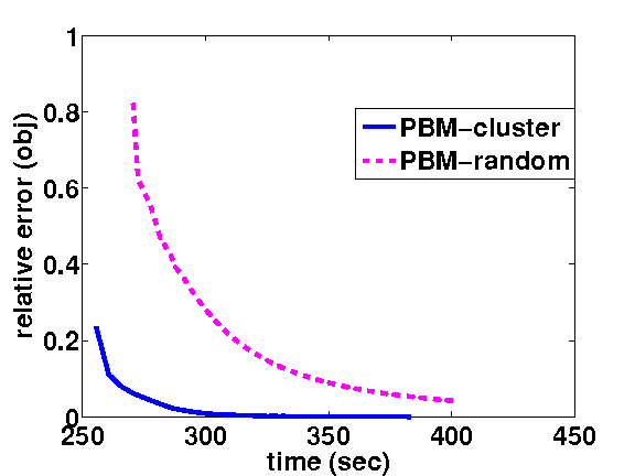
(a) webspam obj

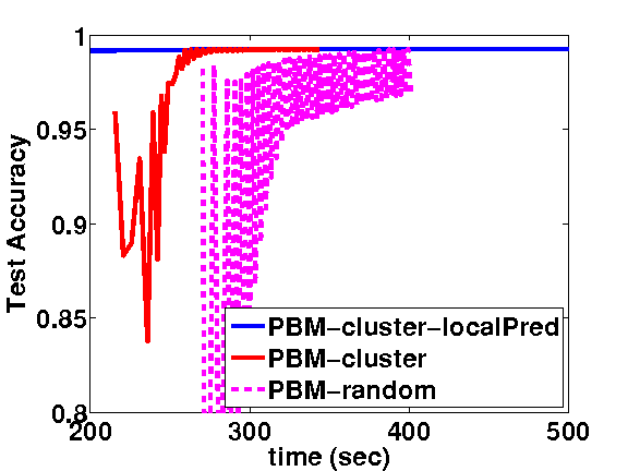
(b) webspam accuracy

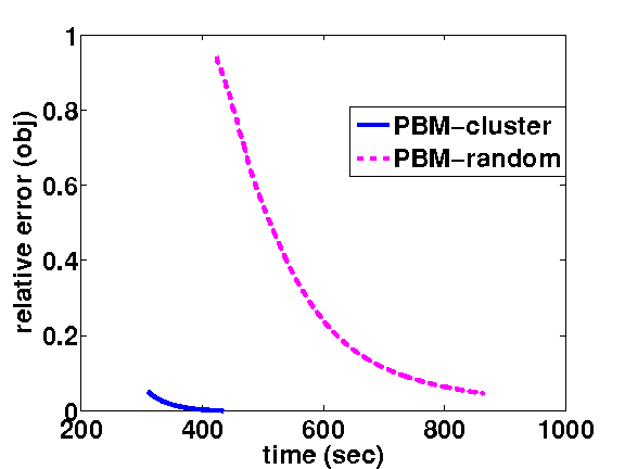
(c) covtype obj

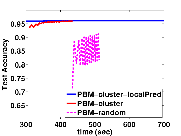
(d) covtype accuracy

Figure 1: Comparison of different variances of PBM. We observe PBM with kmeans partitioning converges faster than random partition, and the accuracy can further be improved by using our local prediction heuristic.

Optimal step size selection. If each $g_{i}$ is a linear function with bounded constraint (such as for the kernel SVM case), the optimal step size can be computed without communication. The optimal step size is defined by

$$\beta^{*}_{t}:=\arg\min_{\beta}f(\boldsymbol{\alpha}+\beta\boldsymbol{d})\text{ s.t. }{\boldsymbol{a}}\leq\boldsymbol{\alpha}+\beta\boldsymbol{d}\leq\boldsymbol{b}.$$ (12)

If $\sum_{i}g_{i}(\alpha_{i})={\boldsymbol{p}}\boldsymbol{\alpha}$, then $f(\boldsymbol{\alpha}+\beta\boldsymbol{d})$ with respect to $\beta$ is a univariate quadratic function, and thus $\beta^{*}_{t}$ can be obtained by the following closed form solution:

$$\beta=\min(\bar{\eta},\max(\underline{\eta},-(\boldsymbol{\alpha}^{T}Q\boldsymbol{d}+{\boldsymbol{p}}^{T}\boldsymbol{d})/(\boldsymbol{d}^{T}Q\boldsymbol{d}))),$$ (13)

where $\bar{\eta}:=\min_{i=1}^{n}(b_{i}-\alpha_{i})$ and $\underline{\eta}:=\max_{i=1}^{n}(a_{i}-\alpha_{i})$. This can also be computed in $O(n/k)$ time and $O(1)$ communication time. Our proposed algorithm is summarized in Algorithm 1.

Input : The objective function (1), initial $\boldsymbol{\alpha}_{0}$.

Output : The solution $\boldsymbol{\alpha}^{*}$.

1 Obtain a disjoint index partition $\{S_{r}\}_{r=1}^{k}$.

2 Compute $Q\boldsymbol{\alpha}_{0}$ in parallel ($Q\boldsymbol{\alpha}_{0}={\boldsymbol{0}}$ if $\boldsymbol{\alpha}_{0}=0$).

3 for $t=0,1,\ldots$(until convergence) do

4       Obtain $\boldsymbol{d}_{S_{r}}$ by solving subproblems (7) in parallel.

5       Compute $Q_{:,S_{r}}\boldsymbol{d}_{S_{r}}$ in parallel.

6       Use Reduce_Scatter to obtain $(Q\boldsymbol{d})_{S_{r}}$ in each worker.

7       Obtain the step size $\beta$ using line search (see Section 4.2 for details)

8       $\boldsymbol{\alpha}_{S_{r}}\leftarrow\boldsymbol{\alpha}_{S_{r}}+\beta\boldsymbol{d}_{S_{r}}$ and $(Q\boldsymbol{\alpha})_{S_{r}}\leftarrow(Q\boldsymbol{\alpha})_{S_{r}}+\beta(Q\boldsymbol{d})_{S_{r}}$ in parallel.

9      

Algorithm 1 PBM: Parallel Block Minimization for solving (1)

4.3 Variable Partitioning

Our PBM algorithm converges for any choice of partition $\{S_{r}\}_{r=1}^{k}$. However, it is important to select a good partition in order to achieve faster convergence. Note that if $\bar{Q}=Q$ in subproblem (4), then $\bar{f}_{\boldsymbol{\alpha}}(\Delta\boldsymbol{\alpha})=f(\boldsymbol{\alpha}+\Delta\boldsymbol{\alpha})$, so the algorithm converges in one iteration. Therefore, to achieve faster convergence, we want to minimize the difference between $\bar{f}_{\boldsymbol{\alpha}}(\Delta\boldsymbol{\alpha})$ and $f(\boldsymbol{\alpha}+\Delta\boldsymbol{\alpha})$, and this can be solved by finding a partition $\{S_{r}\}_{r=1}^{k}$ to minimize error $\|\bar{Q}-Q\|_{F}^{2}=\sum\nolimits_{i,j}Q_{ij}^{2}-\sum\nolimits_{r=1}^{k}\sum\nolimits_{i,j\in S_{r}}Q_{ij}^{2},$ and the minimizer can be obtained by maximizing the second term. However, we also want to have a balanced partition in order to achieve better parallelization speedup.

The same problem has been encountered in [22, 10] for forming a good kernel approximation. They have shown that kernel kmeans can achieve a good partition for general kernel matrix, and if the kernels are shift-invariant (e.g., Gaussian, Laplacian, …), we can use kmeans clustering on the data points to find a balanced partition with small kernel approximation error. Since we do not need the “optimal” partition, in practice we only run kmeans or kernel kmeans on a subset of 20000 training samples, so the overhead is very small compared with the whole training procedure.

We observe PBM with kmeans partition converges much faster compared to random partition. In Figure 1, we test the PBM algorithm on the kernel SVM problem with Gaussian kernel, and show that the convergence is much faster when the partition is obtained by kmeans clustering.

Local Prediction. Inspired by the early prediction strategy discussed in [10], we propose a local prediction strategy for PBM when data is partitioned by kmeans clustering. Let $\boldsymbol{\alpha}_{t}$ be the solution before the $t$-th iteration of Algorithm 1, and $\boldsymbol{d}_{t}$ be the solution of the quadratic subproblem (4). The traditional way is to use $\boldsymbol{\alpha}_{t+1}=\boldsymbol{\alpha}_{t}+\beta_{t}\boldsymbol{d}_{t}$ for predicting new data.

However, we find the following procedure gives better prediction accuracy compared to using $\boldsymbol{\alpha}_{t+1}$: we first identify the cluster indicator of the test point ${\boldsymbol{x}}$ by choosing the nearest kmeans center. If ${\boldsymbol{x}}$ belongs to the $r$-th cluster, we then compute the prediction by the local model $\boldsymbol{\alpha}_{t}+(\boldsymbol{d}_{t})_{<S_{r}>}$, where $(\boldsymbol{d}_{t})_{<S_{r}>}$ is an $n$ dimensional vector that sets all the elements outside $S_{r}$ to be 0. Experimental results in Figure 1 show that this local prediction strategy is generally better than predicting by $\boldsymbol{\alpha}_{t+1}$. The main reason is that during the optimization procedure each local machine fits the local data by $\boldsymbol{\alpha}_{t}+(\boldsymbol{d}_{t})_{<S_{r}>}$, so the prediction accuracy is better than the global model.

Summary: Computational and Memory Cost: In Section 4.1, we showed that the greedy coordinate descent solver only requires $O(|S_{r}|)$ time complexity per inner iteration. Before communication, we need to compute $Q_{:,S_{r}}\boldsymbol{d}_{S_{r}}$ in each machine, which requires $O(tn)$ time complexity, where $t$ is number of inner iterations. The line search requires only $O(n/k)$ time. Therefore, the overall time complexity is $O(tn)$ for totally $O(tk)$ coordinate updates from all workers, so the average time per update is $O(n/k)$, which is $k$ times faster than the original greedy coordinate descent (or SMO) algorithm for kernel SVM, where $k$ is number of machines.

The time for running kmeans is $O(\bar{n}\bar{d})$ using $k$ computers, where $\bar{n}$ is number subsamples (we set it to 20,000). This is a one time cost and is very small comparing to the cost of solving kernel machines. For example, on Covtype dataset the kmeans step only took 13 seconds, while the overall training time is 772 seconds. Note that we include the clustering time in all the experimental results.

Memory Cost: In kernel SVM, the main memory bottleneck is the memory needed for storing the kernel matrix. Without any trick (such as shrinking) to reduce the kernel storage, the space complexity is $O(n^{2})$ for kernel SVM (otherwise we have to recompute kernel values when needed). Using our approach, (1) the subproblem solver only requires $O(n^{2}/k^{2})$ space for the sub-matrix of kernel $Q_{S_{r},S_{r}}$ (2) Before synchronization, computing $Q_{:,S_{r}}\boldsymbol{d}_{S_{r}}$ requires $O(n^{2}/k)$ kernel entries. Therefore, the memory requirement will be reduced from $n^{2}$ to $n^{2}/k$ using our algorithm. However, for large datasets the memory is still not enough. Therefore, similar to the LIBSVM software, we maintain a kernel cache to store columns of $Q$, and maintain the cache using the Least Recent Used (LRU) policy. In short, if memory is not enough, we use the kernel caching technique (implemented in LIBSVM) that computes the kernel values on-the-fly when it is not in the kernel cache and maintains recently used values in memory.

If each machine contains all the training samples, then $Q_{:,S_{r}}\boldsymbol{d}_{S_{r}}$ can be computed in parallel without any communication, and we only need one REDUCE_SCATTER mpi operation to gather the results. However, if each machine only contains a subset of samples, they have to broadcast $\{{\boldsymbol{x}}_{i}\mid i\in S_{r},d_{i}\neq 0\}$ to other machines so that each machine $q$ can compute $(Q\boldsymbol{d})_{S_{q}}$. In this case, we do not need to store the whole training data in each machine, and the communication time will be proportional to number of support vectors, which is usually much smaller than $n$.

5 Convergence Analysis

In this section we show that PBM has a global linear convergence rate under certain mild conditions. Note that our result is stronger than some recent theoretical analysis of distributed coordinate descent. Compared to [5], we show linear convergence even when the objective function (1) is not strictly positive definite (e.g., for SVM with hinge loss), while  [5] only has sub-linear convergence rate for those cases. In comparing to [7], they assume that the subproblems in each worker are solved exactly, while we allow an approximate subproblem solver (e.g., coordinate descent with $\geq 1$ steps).

First we assume the objective function satisfies the following property:

Definition 1.

Problem (1) admits a “global error bound” if there is a constant $\kappa$ such that

$$\|\boldsymbol{\alpha}-P_{S}(\boldsymbol{\alpha})\|\leq\kappa\|T(\boldsymbol{\alpha})-\boldsymbol{\alpha}\|,$$ (14)

where $P_{S}(\cdot)$ is the Euclidean projection to the set $S$ of optimal solutions, and $T:\mathbb{R}^{n}\rightarrow\mathbb{R}^{n}$ is the operator defined by

$$T_{i}(\boldsymbol{\alpha})=\arg\min_{u}f(\boldsymbol{\alpha}+(u-\alpha_{i}){\boldsymbol{e}}_{i}),\ \ \forall i=1,\dots,n.$$ (15)

where ${\boldsymbol{e}}_{i}$ is the standard $i$-th unit vector. We say that the algorithm satisfies a global error bound from the beginning if (14) holds for the level set $\{\boldsymbol{\alpha}\mid f(\boldsymbol{\alpha})\leq f({\boldsymbol{0}})\}$.

The definition is similar to [23, 24]. It has been shown in  [23, 24] that the global error bound assumption covers many widely used machine learning functions. Any strongly convex function satisfies this definition, and in those cases, $\kappa$ is the condition number. Next, we discuss some problems that admit a global error bound:

Corollary 1.

The algorithm for solving (1) satisfies a global error bound from the beginning if one of the following conditions is true.

• $Q$ is positive definite (kernel is positive definite).

• For all $i=1,\dots,n$, $g_{i}(\cdot)$ is strongly convex for all the iterates (e.g., dual $\ell_{2}$-regularized logistic regression with positive semi-definite kernel).

• $Q$ is positive semi-definite and $g_{i}(\cdot)$ is linear for all $i$ with a box constraint (e.g., dual hinge loss SVM with positive semi-definite kernel).

Corollary 1 implies that many widely used machine learning problems, including dual formulation of SVM and $\ell_{2}$-regularized logistic regression, admit a global error bound from the beginning even when the kernel has a zero eigenvalue.

We do not require the inner solver to obtain the exact solution of (7). Instead, we define the following condition for the inexact inner solver.

Definition 2.

An inexact solver for solving the subproblem (7) achieves a “local linear improvement” if the inexact solution $\boldsymbol{d}_{S_{r}}$ satisfies

$$E[f_{\boldsymbol{\alpha}}^{(r)}(\boldsymbol{d}_{S_{r}})]-f_{\boldsymbol{\alpha}}^{(r)}(\hat{\boldsymbol{d}}_{S_{r}})\leq\eta\big{(}f_{\boldsymbol{\alpha}}^{(r)}({\boldsymbol{0}})-f_{\boldsymbol{\alpha}}^{(r)}(\hat{\boldsymbol{d}}_{S_{r}})\big{)},$$ (16)

for all iterates, where $f_{\boldsymbol{\alpha}}^{(r)}$ is the subproblem defined in (7), $\hat{\boldsymbol{d}}_{S_{r}}:=\arg\min_{\Delta}f_{\boldsymbol{\alpha}}^{(r)}(\Delta)$ is the optimal solution of the subproblem, and $\eta\in(0,1)$ is a constant. Note that we can drop the expectation when the solver is deterministic.

In the following we list some widely-used subproblem solvers that satisfy Definition 2.

Corollary 2.

The following subproblem solvers satisfy Definition 2 if the objective function admits a global error bound from the beginning: (1) Greedy Coordinate Descent with at least one step. (2) Stochastic coordinate descent with at least one step. (3) Cyclic coordinate descent with at least one epoch.

The condition of (16) will be satisfied if an algorithm has a global linear convergence rate. The global linear convergence rate of cyclic coordinate descent has been proved in Section 3 of [24]. We show global linear convergence for randomized coordinate descent and greedy coordinate descent in the Appendix.

We now show our proposed method PBM in Algorithm 1 has a global linear convergence rate in the following theorem.

Theorem 1.

Assume (1) the objective function admits a global error bound from the beginning (Definition 1), (2) the inner solver achieves a local linear improvement (Definition 2), (3) $R_{min}=\min_{i}Q_{ii}\neq 0$, and (4) the objective function is $L$-Lipschitz continuous for the level set. Then the following global linear convergence rate holds:

$$E[f(\boldsymbol{\alpha}_{t+1})]-f(\boldsymbol{\alpha}^{*})\leq\big{(}1-(1-\eta)R_{min}/(kBL\kappa^{2})\big{)}\big{(}E[f(\boldsymbol{\alpha}_{t})]-f(\boldsymbol{\alpha}^{*})\big{)},$$

where $\boldsymbol{\alpha}^{*}$ is an optimal solution, and $B=\max_{r=1}^{k}|S_{r}|$ is the maximum block size. We can drop the expectation when the solver is deterministic.

Proof.

We first define some notations that we will use in the proof. Let $\boldsymbol{\alpha}_{t}$ be the current solution of iteration $t$, $\boldsymbol{d}_{t}$ is the approximate solution of (7) satisfying Definition 2. For convenience we will omit the subscript $t$ here (so $\boldsymbol{d}:=\boldsymbol{d}_{t}$). We use $\boldsymbol{d}_{S_{r}}$ to denote the size $|S_{r}|$ subvector, and $\boldsymbol{d}_{<S_{r}>}$ to denote the $n$ dimensional vector with

$$\boldsymbol{d}_{<S_{r}>}=\begin{cases}d_{i}&\text{ if }i\in S_{r}\\ 0&\text{ otherwise}\end{cases}$$

By the definition of our line search procedure described in Section 4.2, we have

$$f(\boldsymbol{\alpha}_{t}+\beta\boldsymbol{d}) \leq f(\boldsymbol{\alpha}_{t}+\frac{1}{k}\sum_{r=1}^{k}\boldsymbol{d}_{<S_{r}>})$$

$$=f(\frac{1}{k}\sum_{r=1}^{k}(\boldsymbol{\alpha}_{t}+\boldsymbol{d}_{<S_{r}>}))$$

$$\leq\frac{1}{k}\sum_{r=1}^{k}f(\boldsymbol{\alpha}_{t}+\boldsymbol{d}_{<S_{r}>}),$$

where the last inequality is from the definition is from the convexity of $f(\cdot)$. We define $\hat{\boldsymbol{d}}$ to be the optimal solution of (4) (so each $\hat{\boldsymbol{d}}_{S_{r}}$ is the optimal solution of the $r$-th subproblem (7)). Then we have

$$f(\boldsymbol{\alpha}_{t})-f(\boldsymbol{\alpha}_{t}+\boldsymbol{d}_{t})$$ (17)

$$\geq f(\boldsymbol{\alpha}_{t})-\frac{1}{k}\sum_{r=1}^{k}f(\boldsymbol{\alpha}_{t}+\boldsymbol{d}_{<S_{r}>})$$

$$= \frac{1}{k}\sum_{r=1}^{k}(f(\boldsymbol{\alpha}_{t})-f(\boldsymbol{\alpha}_{t}+\boldsymbol{d}_{<S_{r}>}))$$

$$= \frac{1}{k}\sum_{r=1}^{k}\bigg{(}f(\boldsymbol{\alpha}_{t})-f(\boldsymbol{\alpha}_{t}+\hat{\boldsymbol{d}}_{<S_{r}>})$$

$$+f(\boldsymbol{\alpha}_{t}+\hat{\boldsymbol{d}}_{<S_{r}>})-f(\boldsymbol{\alpha}_{t}+\boldsymbol{d}_{<S_{r}>})\bigg{)}$$

$$\geq \frac{1}{k}\sum_{r=1}^{k}(1-\eta)\bigg{(}f(\boldsymbol{\alpha}_{t})-f(\boldsymbol{\alpha}_{t}+\hat{\boldsymbol{d}}_{<S_{r}>})\bigg{)},$$ (18)

where the last inequality is from the local linear improvement of the in-exact subproblem solver (Definition 2). We then define a vector $\bar{\boldsymbol{d}}$ where each element is the optimal solution of the one variable subproblem:

$$\bar{d}_{i}=T_{i}(\boldsymbol{\alpha}_{t})-(\boldsymbol{\alpha}_{t})_{i}\ \ \forall i=1,\dots,n,$$

where $T_{i}(\boldsymbol{\alpha}_{t})$ was defined in (15).

Since $\hat{\boldsymbol{d}}_{S_{r}}$ is the optimal solution of each subproblem, we have

$$f(\boldsymbol{\alpha}_{t}+\hat{\boldsymbol{d}}_{<S_{r}>})\leq f(\boldsymbol{\alpha}_{t}+\bar{\boldsymbol{d}}_{<S_{r}>}),\ \forall r=1,\dots,k.$$

Combining with (18) we get

$$f(\boldsymbol{\alpha}_{t})-f(\boldsymbol{\alpha}_{t}+\boldsymbol{d}_{t})$$

$$\geq \frac{1-\eta}{k}\sum_{r=1}^{k}\big{(}f(\boldsymbol{\alpha}_{t})-f(\boldsymbol{\alpha}_{t}+\bar{\boldsymbol{d}}_{<S_{r}>})\big{)}$$

$$\geq \frac{1-\eta}{k}\sum_{r=1}^{k}\bigg{(}f(\boldsymbol{\alpha}_{t})-f\big{(}\frac{1}{|S_{r}|}\sum_{i\in S_{r}}(\boldsymbol{\alpha}_{t}+\bar{\boldsymbol{d}}_{<i>})\big{)}\bigg{)}$$

$$\geq \frac{1-\eta}{k}\sum_{r=1}^{k}\bigg{(}f(\boldsymbol{\alpha}_{t})-\frac{1}{|S_{r}|}\sum_{i\in S_{r}}f(\boldsymbol{\alpha}_{t}+\bar{\boldsymbol{d}}_{<i>})\bigg{)}$$

(by the convexity of $$f$$)

$$= \frac{1-\eta}{k}\sum_{r=1}^{k}\frac{1}{|S_{r}|}\sum_{i\in S_{r}}\big{(}f(\boldsymbol{\alpha}_{t})-f(\boldsymbol{\alpha}_{t}+\bar{\boldsymbol{d}}_{<i>})\big{)}$$

$$\geq \frac{1-\eta}{kB}\sum_{i=1}^{n}\big{(}f(\boldsymbol{\alpha}_{t})-f(\boldsymbol{\alpha}_{t}+\bar{\boldsymbol{d}}_{<i>})\big{)},$$

where the last inequality is by the definition of $B$.

Now consider the one variable problem $f(\boldsymbol{\alpha}_{t}+u{\boldsymbol{e}}_{i})$. By Taylor expansion and the definition of $R_{min}$ we have

$$f(\boldsymbol{\alpha}_{t}) \geq f(\boldsymbol{\alpha}_{t}+\bar{\boldsymbol{d}}_{<i>})+\partial_{i}f(\boldsymbol{\alpha}_{t}+\bar{\boldsymbol{d}}_{<i>})\times\bar{d}_{i}+\frac{1}{2}R_{min}\bar{d}_{i}^{2}$$

$$\geq f(\boldsymbol{\alpha}_{t}+\bar{\boldsymbol{d}}_{<i>})+\frac{1}{2}R_{min}\bar{d}_{i}^{2},$$

where the second inequality comes from the fact that $\bar{d}_{i}$ is the optimal solution of the one-variable subproblem. As a result,

$$\sum_{i=1}^{n}\bigg{(}f(\boldsymbol{\alpha}_{t})-f(\boldsymbol{\alpha}_{t}+\bar{\boldsymbol{d}}_{<i>})\bigg{)}\geq\sum_{i=1}^{n}R_{min}\bar{d}_{i}^{2}=R_{min}\|\bar{\boldsymbol{d}}\|^{2}.$$

Therefore,

$$f(\boldsymbol{\alpha}_{t})-f(\boldsymbol{\alpha}_{t}+\boldsymbol{d}_{t}) \geq\frac{R_{min}(1-\eta)}{kB}\|\bar{\boldsymbol{d}}\|^{2}$$

$$=\frac{R_{min}(1-\eta)}{kB}\|T(\boldsymbol{\alpha}_{t})-\boldsymbol{\alpha}_{t}\|^{2}$$

$$\geq\frac{R_{min}(1-\eta)}{kB\kappa^{2}}\|P_{S}(\boldsymbol{\alpha}_{t})-\boldsymbol{\alpha}_{t}\|^{2}\text{ (by~{}\eqref{eq:global_error})}$$

$$\geq\frac{LR_{min}(1-\eta)}{kB\kappa^{2}}\|f(\boldsymbol{\alpha}_{t})-f(\boldsymbol{\alpha}^{*})\|.$$

Therefore, we have

$$f(\boldsymbol{\alpha}_{t+1})-f(\boldsymbol{\alpha}^{*}) =f(\boldsymbol{\alpha}_{t})-\big{(}f(\boldsymbol{\alpha}_{t})-f(\boldsymbol{\alpha}_{t+1})\big{)}-f(\boldsymbol{\alpha}^{*})$$

$$\leq\bigg{(}1-\frac{R_{min}(1-\eta)}{kBL\kappa^{2}}\bigg{)}\big{(}f(\boldsymbol{\alpha}_{t})-f(\boldsymbol{\alpha}^{*})\big{)}.$$

∎

Note that we do not make any assumption on the partition used in PBM, so our analysis works for a wide class of optimization solvers, including distributed linear SVM solver in [7] where they only consider that case when the subproblems are solved exactly.

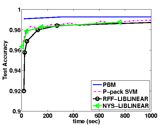
(a) webspam, comparison

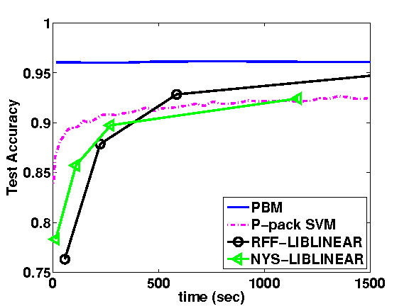
(b) covtype, comparison

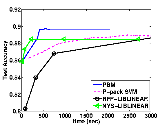
(c) cifar, comparison

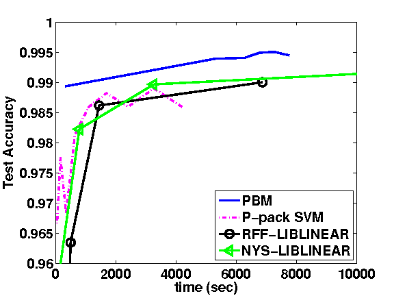
(d) mnist8m, comparison

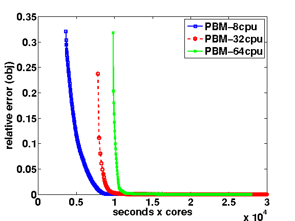
(e) webspam, scaling

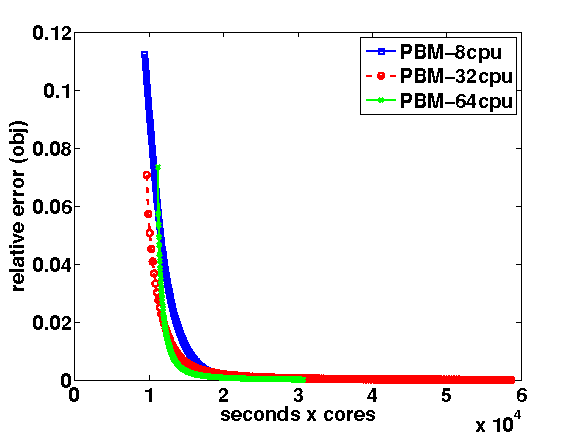
(f) covtype, scaling

Figure 2: (a)-(d): Comparison with other distributed kernel SVM solvers using 32 workers. Markers for RFF-LIBLINEAR and NYS-LIBLINEAR are obtained by varying the number random features and landmark points respectively. (e)-(f): The objective function of PBM as a function of computation time (time in seconds $\times$ the number of workers), when the number of workers is varied. Results show that PBM has good scalability.

Table 1: Dataset statistics

Dataset	# training samples	# testing samples	# features	$C$	$\gamma$
cifar	50,000	10,000	3072	$2^{3}$	$2^{-22}$
covtype	464,810	116,202	54	$2^{5}$	$2^{5}$
webspam	280,000	70,000	254	$2^{3}$	$2^{5}$
mnist8m	8,000,000	100,000	784	$2^{0}$	$2^{-21}$
kdda	8,407,752	510,302	20,216,830	$2^{0}$	$2^{-15}$

Table 2: Comparison on real datasets. We use 32 machines for all the distributed solvers (PBM, P-packSGD, PSVM), and 1 machine for the serial solver (DC-SVM). The first column of PBM shows that PBM achieves good test accuracy after 1 iteration, and the second column of PBM shows PBM can achieve an accurate solution (with $\frac{f(\boldsymbol{\alpha})-f(\boldsymbol{\alpha}^{*})}{|f(\boldsymbol{\alpha}^{*})|}<10^{-3}$) quickly and obtain even better accuracy. Note that “-” indicates the training time is more than 10 hours and “x” indicates the algorithm cannot solve logistic regression. The timing for kernel logistic regression (LR) is much slower because $\boldsymbol{\alpha}$ is always dense when using the logistic loss. Although DC-SVM and PSVM can be potentially used for logistic regression, there is no existing implementation for these methods. Writing good code for logistic regression is nontrivial—we have to do kernel caching and shrinking for large datasets. Therefore we do not compare with them here.

	PBM (first step)		PBM ($10^{-3}$ error)		P-packSGD		PSVM $p=n^{0.5}$		PSVM $p=n^{0.6}$		DC-SVM ($10^{-3}$ error)
	time(s)	acc(%)	time(s)	acc(%)	time(s)	acc(%)	time(s)	acc(%)	time(s)	acc(%)	time(s)	acc(%)
webspam (SVM)	16	99.07	360	99.26	1478	98.99	773	75.79	2304	88.68	8742	99.26
covtype (SVM)	14	96.05	772	96.13	1349	92.67	286	76.00	7071	81.53	10457	96.13
cifar (SVM)	15	85.91	540	89.72	1233	88.31	41	79.89	1474	69.73	13006	89.72
mnist8m (SVM)	321	98.94	8112	99.45	2414	98.60	-	-	-	-	-	-
kdda (SVM)	1832	85.51	12700	86.31	-	-	-	-	-	-	-	-
webspam (LR)	1679	92.01	2131	99.07	4417	98.96	x	x	x	x	x	x
cifar (LR)	471	83.37	758	88.14	2115	87.07	x	x	x	x	x	x

6 Experimental Results

We conduct experiments on five large-scale datasets listed in Table 1. We follow the procedure in [25, 10] to transform cifar and mnist8m into binary classification problems, and Gaussian kernel $K({\boldsymbol{x}}_{i},{\boldsymbol{x}}_{j})=e^{-\gamma\|{\boldsymbol{x}}_{i}-{\boldsymbol{x}}_{j}\|^{2}}$ is used in all the comparisons. We follow the parameter settings in [10], where $C$ and $\gamma$ are selected by 5-fold cross validation on a grid of parameters. The experiments are conducted on Texas Advanced Computing Center Maverick cluster.

We compare our PBM method with the following distributed kernel SVM training algorithms:

1. P-pack SVM [4]: a parallel Stochastic Gradient Descent (SGD) algorithm for kernel SVM training. We set the pack size $r=100$ according to the original paper.

2. Random Fourier features with distributed LIBLINEAR: In a distributed system, we can compute random features [13] for each sample in parallel (this is a one-time preprocessing step), and then solve the resulting linear SVM problem by distributed dual coordinate descent [7] implemented in MPI LIBLINEAR. Note that although Fastfood [26] can generate random features in a faster way, the bottleneck for RFF-LIBLINEAR is solving the resulting linear SVM problem after generating random features, so the performance is similar.

3. Nyström approximation with distributed LIBLINEAR: We implemented the ensemble Nyström approximation [27] with kmeans sampling in a distributed system and solved the resulting linear SVM problem by MPI LIBLINEAR. The approach is similar to [28].

4. PSVM [3]: a parallel kernel SVM solver by in-complete Cholesky factorization and a parallel interior point method. We test the performance of PSVM with the rank suggested by the original paper ($n^{0.5}$ or $n^{0.6}$ where $n$ is number of samples).

Comparison with other solvers. We use 32 machines (each with 1 thread) and the best $C,\gamma$ for all the solvers. Our parameter settings are exactly the same with  [10] chosen by cross-validation in $[2^{-30},2^{10}]$. For cifar, mnist8m and kdda the samples are not normalized, so the averaged norm mean($\|{\boldsymbol{x}}_{i}\|$) is large (it is 876 on cifar). Since Gaussian kernel is $e^{-\gamma\|{\boldsymbol{x}}_{i}-{\boldsymbol{x}}_{j}\|^{2}}$, a good $\gamma$ will be very small. We mainly compare the prediction accuracy in the paper because most of the parallel kernel SVM solvers are “approximate solvers”—they solve an approximated problem, so it is not fair to evaluate them using the original objective function. The results in Figure 2 (a)-(d) indicate that our proposed algorithm is much faster than other approaches. We further test the algorithms with varied number of workers and parameters in Table 2. Note that PSVM usually gets lower test accuracy so we only show its results in Table 2.

Scalability of PBM. For the second experiment we varied the number of workers from 8 to 64, and plot the scaling behavior of PBM. In Figure 2 (e)-(f), we set $y$-axis to be the relative error defined by $(f(\boldsymbol{\alpha}_{t})-f(\boldsymbol{\alpha}^{*}))/f(\boldsymbol{\alpha}^{*})$ where $\boldsymbol{\alpha}^{*}$ is the optimal solution, and $x$-axis to be the total CPU time expended which is given by the number of seconds elapsed multiplied by the number of workers. We plot the convergence curves by changing number of cores. The perfect linear speedup is achieved until the curves overlap. This is indeed the case for covtype.

Comparison with single-machine solvers. We also compare PBM with state-of-the-art sequential kernel SVM algorithm DC-SVM [10]. The results are in Table 2 and Figure 3. DC-SVM first computes the solutions in each partition, and then use the concatenation of local (dual) solutions to initialize a global kernel SVM solver (e.g., LIBSVM). However, the top level of DC-SVM is the bottleneck (taking 2/3 of the run time), and LIBSVM cannot run on multiple machines. So DC-SVM cannot be parallelized, and we compare our method with it just to show our distributed algorithm is much faster than the best serial algorithm (which is not the case for many other distributed solvers).

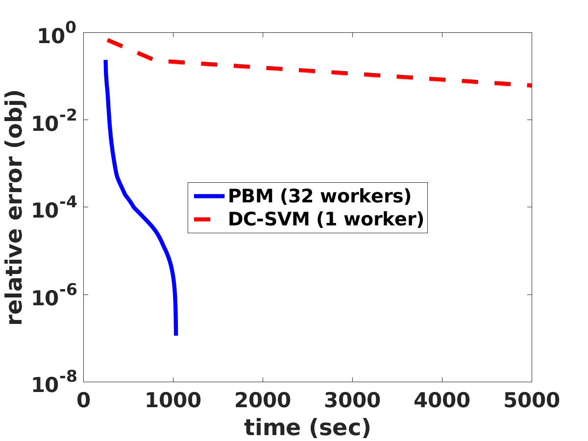
(a) webspam, obj

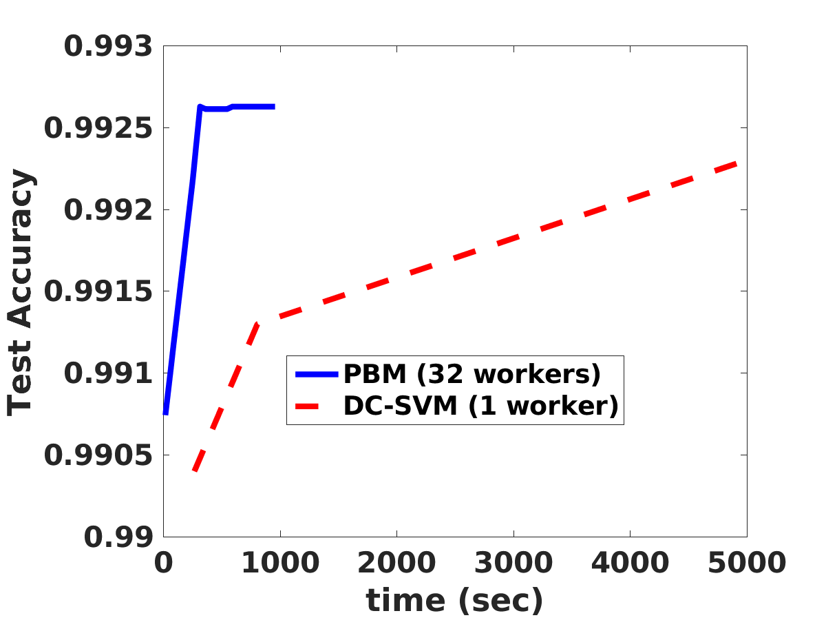
(b) webspam, accuracy

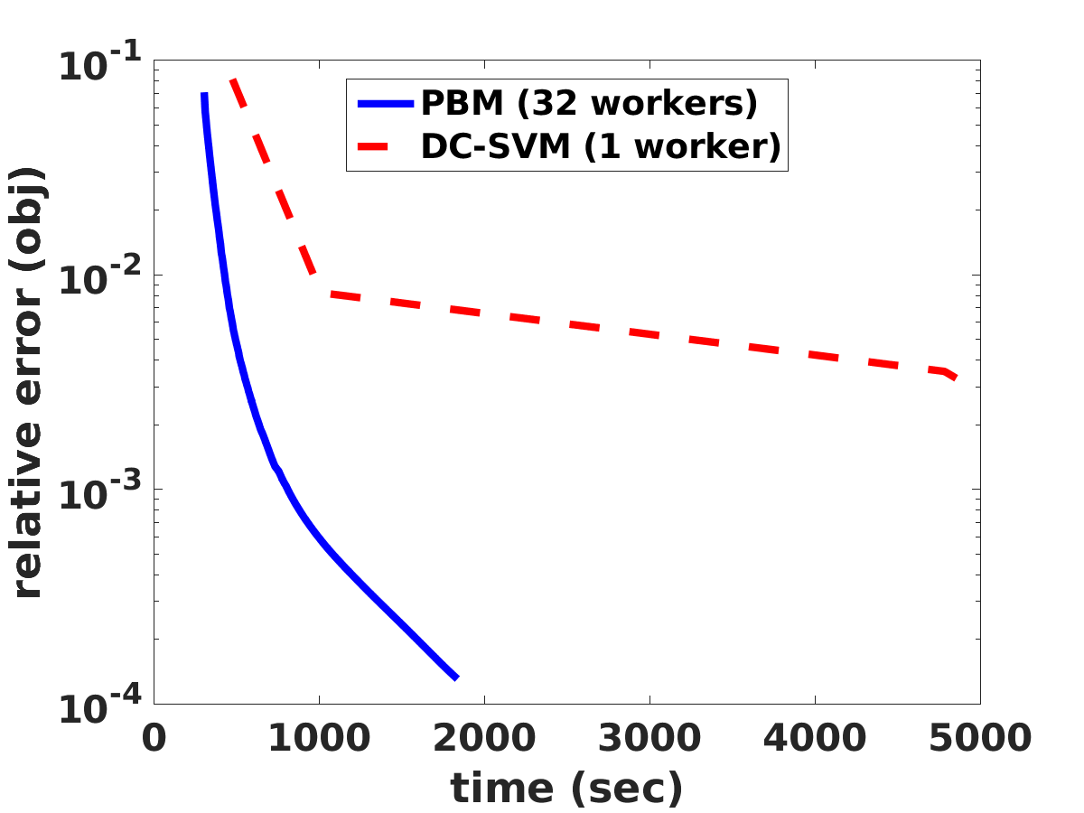
(c) covtype, obj

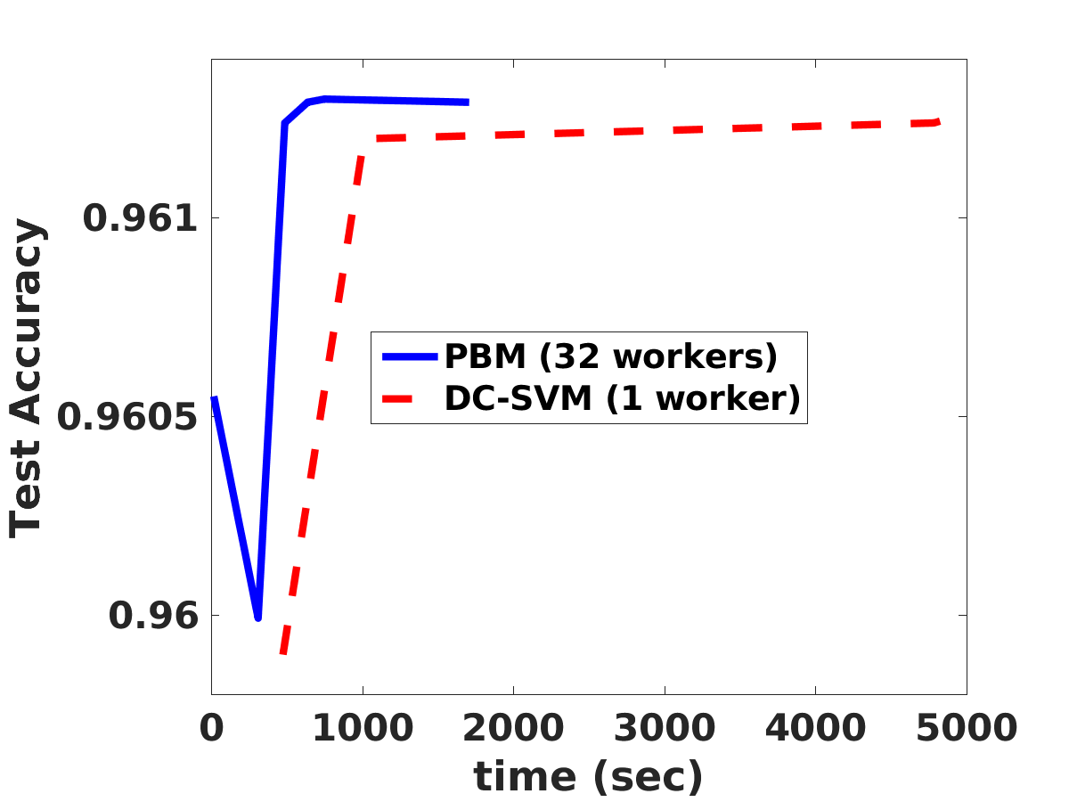
(d) covtype, accuracy

Figure 3: Comparison with DC-SVM (a sequential kernel SVM solver).

Kernel logistic regression. We implement the PBM algorithm to solve the kernel logistic regression problem. Note that PSVM cannot be directly applied to kernel logistic regression. We use greedy coordinate descent proposed in [8] to solve each subproblem (7). The results are presented in Table 2, showing that our algorithm is faster than others.

7 Conclusion

We have proposed a parallel block minimization (PBM) framework for solving kernel machines on distributed systems. We show that PBM significantly outperforms other approaches on large-scale datasets, and prove a global linear convergence of PBM under mild conditions.

8 Proof of Corollary 2

The condition of (16) will be satisfied if an algorithm has a global linear convergence rate. The global linear convergence rate of cyclic coordinate descent has been proved in Section 3 of [24]. We show global linear convergence for Randomized Coordinate Descent (RCD) and Greedy Coordinate Descent (GCD) in the following. In the following we focus on solving the following $n$-variate optimization problem by RCD and GCD:

$$\min_{{\boldsymbol{x}}\in\mathbb{R}^{n}}f({\boldsymbol{x}}),$$

and we further assume (1) $f(\cdot)$ satisfies the global error bound assumption (Definition 1), and (2) Each single-variable subproblem $g_{i}(s)=f({\boldsymbol{x}}+s{\boldsymbol{e}}_{i})$ is $R_{min}$-strongly convex on $s$ for any ${\boldsymbol{x}}$, and $R_{min}>0$, and (3) $f(\cdot)$ has $L$-Lipchitz continuous gradient. Clearly the first assumption is satisfied for the subproblem we considered in this paper with $R_{min}=\min_{i}q_{ii}$.

8.1 Local Linear Improvement for Randomized Coordinate Descent

We first formally describe the procedure of Randomized Coordinate Descent (RCD). The RCD algorithm can be written below:

• For $t=0,1,\dots$

  1. Select an index $i(t)$ uniformly random from $\{1,2,\dots,n\}$

  2. Compute $\delta_{t}$ by

     $$\delta_{t}\leftarrow T_{i(t)}(\boldsymbol{\alpha}^{t}),$$

     where $T_{i(t)}(\boldsymbol{\alpha}^{t})$ was defined in (15).

  3. Update $\boldsymbol{\alpha}^{t+1}\leftarrow\boldsymbol{\alpha}^{t}+(\delta_{t}-\alpha^{t}_{i(t)}){\boldsymbol{e}}_{i(t)}$.

At each iteration, RCD selects a coordinate randomly and update it by solving the single variable subproblem exactly. Now we show a global linear convergence rate of RCD. Taking $t=1$ in the following theorem we can see RCD satisfies Definition 2.

Theorem 2.

The sequence $\{\boldsymbol{\alpha}^{t}\}$ generated by RCD satisfies

$$\bigg{(}E[f(\boldsymbol{\alpha}^{t})]-f(\boldsymbol{\alpha}^{*})\bigg{)}\leq\bigg{(}1-\frac{R_{min}}{2nL\kappa^{2}}\bigg{)}^{t}\bigg{(}E[f(\boldsymbol{\alpha}^{0})]-f(\boldsymbol{\alpha}^{*})\bigg{)},$$

where $\kappa$ is the parameter in the global error bound (14), and $L$ is the Lipschitz constant of the gradient.

Proof.

First, we define another vector $\boldsymbol{\beta}^{t+1}\in\mathbb{R}^{n}$ such that

$$\beta^{t+1}_{j}=\begin{cases}T_{j}(\boldsymbol{\alpha}^{t})&\text{ if }j=i(t)\\ \alpha^{t}_{j}&\text{ if }j\neq i(t).\end{cases}$$

We then have

$$E_{i(t)}[\|\boldsymbol{\alpha}^{t}-\boldsymbol{\beta}^{t+1}\|^{2}] =\sum_{j}\frac{1}{n}(\alpha^{t}_{j}-T_{j}(\boldsymbol{\alpha}^{t}))^{2}$$

$$=\frac{1}{n}\|\boldsymbol{\alpha}^{t}-T(\boldsymbol{\alpha}^{t})\|^{2},$$

where the expectation is taken with respect to the index $i(t)$. Since the single variable function is $Q_{ii}$-strongly convex and $\alpha^{t+1}_{i}=\beta^{t+1}_{i}$ is the optimal solution for the single variable subproblem, we have

$$f(\boldsymbol{\alpha}^{t})-f(\boldsymbol{\alpha}^{t+1}) \geq\frac{Q_{ii}}{2}\|\boldsymbol{\alpha}^{t}-\boldsymbol{\beta}^{t+1}\|^{2}$$

$$\geq\frac{R_{min}}{2}\|\boldsymbol{\alpha}^{t}-\boldsymbol{\beta}^{t+1}\|^{2}.$$

Taking expectation on both sides we have

$$E[f(\boldsymbol{\alpha}^{t})]-E[f(\boldsymbol{\alpha}^{t+1})] \geq\frac{R_{min}}{2n}E[\|T(\boldsymbol{\alpha}^{t})-\boldsymbol{\alpha}^{t}\|^{2}]$$

$$\geq\frac{R_{min}}{2n\kappa^{2}}\|\boldsymbol{\alpha}^{t}-P_{S}(\boldsymbol{\alpha}^{t})\|^{2}$$

$$\geq\frac{R_{min}}{2nL\kappa^{2}}E[f(\boldsymbol{\alpha}^{t})-f(\boldsymbol{\alpha}^{*})]$$

where $\boldsymbol{\alpha}^{*}$ is the optimal solution. Therefore, we have

$$E[f(\boldsymbol{\alpha}^{t})]-E[f(\boldsymbol{\alpha}^{*})]+E[f(\boldsymbol{\alpha}^{*})]-E[f(\boldsymbol{\alpha}^{t+1})]$$

$$\geq \frac{R_{min}}{2nL\kappa^{2}}\bigg{(}E[f(\boldsymbol{\alpha}^{t})]-E[f(\boldsymbol{\alpha}^{*})]\bigg{)}$$

So

$$E[f(\boldsymbol{\alpha}^{t+1})]-f(\boldsymbol{\alpha}^{*})\leq(1-\frac{R_{min}}{2nL\kappa^{2}})\bigg{(}E[f(\boldsymbol{\alpha}^{t})]-E[f(\boldsymbol{\alpha}^{*})]\bigg{)}.$$

∎

8.2 Local Linear improvement for Greedy Coordinate Descent

We formally define the Greedy Coordinate Descent (GCD) updates.

• For $t=1,2,\dots$

  1. Select an index $i(t)$ by

     $$i(t)\leftarrow\arg\min_{i}|T_{i}(\boldsymbol{\alpha}^{t})-\alpha^{t}_{i}|$$

  2. Compute $\delta_{t}$ by

     $$\delta_{t}\leftarrow T_{i(t)}(\boldsymbol{\alpha}^{t}).$$

  3. Update $\boldsymbol{\alpha}^{t+1}\leftarrow\boldsymbol{\alpha}^{t}+(\delta_{t}-\alpha^{t}_{i(t)}){\boldsymbol{e}}_{i(t)}$.

Now we show a global linear convergence rate for greedy coordinate descent. Taking $t=1$ in the following theorem we can see GCD satisfies Definition 2.

Theorem 3.

The sequence $\{\boldsymbol{\alpha}^{t}\}$ generated by GCD satisfies

$$f(\boldsymbol{\alpha}^{t})-f(\boldsymbol{\alpha}^{*})\leq\bigg{(}1-\frac{R_{min}}{2nL\kappa^{2}}\bigg{)}^{t}\bigg{(}f(\boldsymbol{\alpha}^{0})-f(\boldsymbol{\alpha}^{*})\bigg{)},$$

where $\kappa$ is the parameter in the global error bound (14), and $L$ is the Lipschitz constant of the gradient.

Proof.

Since $i(t)$ is the maximum absolute value in $T(\boldsymbol{\alpha}^{t})$, we can derive the following inequalities:

$$f(\boldsymbol{\alpha}^{t})-f(\boldsymbol{\alpha}^{t+1}) \geq\frac{Q_{ii}}{2}(\alpha^{t+1}_{i(t)}-\alpha^{t}_{i(t)})^{2}$$

$$\geq\frac{Q_{ii}}{2}\frac{1}{n}\|T(\boldsymbol{\alpha}^{t})-\boldsymbol{\alpha}^{t}\|^{2}\text{ (by greedy selection rule)}$$

$$\geq\frac{Q_{ii}}{2n\kappa^{2}}\|\boldsymbol{\alpha}^{t}-P_{S}(\boldsymbol{\alpha}^{t})\|^{2}\text{ (global error bound)}$$

$$\geq\frac{R_{min}}{2nL\kappa^{2}}\|f(\boldsymbol{\alpha}^{t})-f(\boldsymbol{\alpha}^{*})\|$$

Therefore, we have

$$f(\boldsymbol{\alpha}^{t+1})-f(\boldsymbol{\alpha}^{*})\leq(1-\frac{R_{min}}{2nL\kappa^{2}})\bigg{(}f(\boldsymbol{\alpha}^{t})-f(\boldsymbol{\alpha}^{*})\bigg{)}.$$

∎

References

- Platt [1998] John C. Platt. Fast training of support vector machines using sequential minimal optimization. In Advances in Kernel Methods - Support Vector Learning, 1998.
- Joachims [1998] Thorsten Joachims. Making large-scale SVM learning practical. In Advances in Kernel Methods – Support Vector Learning, 1998.
- Chang et al. [2008] E. Chang, K. Zhu, H. Wang, H. Bai, J. Li, Z. Qiu, and H. Cui. Parallelizing support vector machines on distributed computers. In NIPS. 2008.
- Zhu et al. [2009] Zeyuan A. Zhu, Weizhu Chen, Gang Wang, Chenguang Zhu, and Zheng Chen. P-packSVM: Parallel primal gradient descent kernel SVM. In ICDM, 2009.
- Jaggi et al. [2014] Martin Jaggi, Virginia Smith, Martin Takáč, Jonathan Terhorst, Thomas Hofmann, and Michael I Jordan. Communication-efficient distributed dual coordinate ascent. In NIPS. 2014.
- Zhang and Xiao [2015] Y. Zhang and L. Xiao. DiSCO: Communication-efficient distributed optimization of self-concordant loss. In ICML, 2015.
- Lee and Roth [2015] C.-P. Lee and D. Roth. Distributed box-constrained quadratic optimization for dual linear SVM. In ICML, 2015.
- Keerthi et al. [2005] S. Sathiya Keerthi, Kaibo Duan, Shirish Shevade, and Aun Neow Poo. A fast dual algorithm for kernel logistic regression. Machine Learning, 61:151–165, 2005.
- Graf et al. [2005] H. P. Graf, E. Cosatto, L. Bottou, I. Dundanovic, and V. Vapnik. Parallel support vector machines: The cascade SVM. In NIPS, 2005.
- Hsieh et al. [2014] C. J. Hsieh, S. Si, and I. S. Dhillon. A divide-and-conquer solver for kernel support vector machines. In ICML, 2014.
- You et al. [2015] Y. You, J. Demmel, K. Czechowski, L. Song, and R. Vuduc. CA-SVM: Communication-avoiding support vector machines on clusters. In IPDPS, 2015.
- Williams and Seeger [2001] C. K. I. Williams and M. Seeger. Using the Nyström method to speed up kernel machines. In NIPS, 2001.
- Rahimi and Recht [2008] Ali Rahimi and Benjamin Recht. Random features for large-scale kernel machines. In NIPS, 2008.
- Huang et al. [2014] P.-S. Huang, H. Avron, T. Sainath, V. Sindhwani, and B. Ramabhadran. Kernel methods match deep neural networks on timit. In ICASSP, pages 205–209, 2014.
- Tu et al. [2016] Stephen Tu, Rebecca Roelofs, Shivaram Venkataraman, and Benjamin Recht. Large scale kernel learning using block coordinate descent. CoRR, abs/1602.05310, 2016.
- Yang [2013] T. Yang. Trading computation for communication: Distributed stochastic dual coordinate ascent. In NIPS, 2013.
- Richtárik and Takáč [2012] P. Richtárik and M. Takáč. Parallel coordinate descent methods for big data optimization. Mathematical Programming, 2012.
- Scherrer et al. [2012] C. Scherrer, A. Tewari, M. Halappanavar, and D. Haglin. Feature clustering for accelerating parallel coordinate descent. In NIPS, 2012.
- Mahajan et al. [2014a] Dhruv Mahajan, S. Sathiya Keerthi, and Sundararajan Sellamanickam. A distributed block coordinate descent method for training l1 regularized linear classifiers. arXiv:1405.4544, 2014a.
- Yu et al. [2011] H.-F. Yu, F.-L. Huang, and C.-J. Lin. Dual coordinate descent methods for logistic regression and maximum entropy models. Machine Learning, 85(1-2):41–75, 2011.
- Chan et al. [2007] E. Chan, M. Heimlich, A. Purkayastha, and R. van de Geijn. Collective communication: Theory, practice, and experience. Concurrency and Computation: Practice and Experience, 19:1749–1783, 2007.
- Si et al. [2014] S. Si, C. J. Hsieh, and I. S. Dhillon. Memory efficient kernel approximation. In ICML, 2014.
- Hsieh et al. [2015] C.-J. Hsieh, H. F. Yu, and I. S. Dhillon. PASSCoDe: Parallel ASynchronous Stochastic dual Coordinate Descent. In ICML, 2015.
- Wang and Lin [2014] P.-W. Wang and C.-J. Lin. Iteration complexity of feasible descent methods for convex optimization. Journal of Machine Learning Research, 15:1523–1548, 2014.
- Zhang et al. [2012] K. Zhang, L. Lan, Z. Wang, and F. Moerchen. Scaling up kernel SVM on limited resources: A low-rank linearization approach. In AISTATS, 2012.
- Le et al. [2013] Q. Le, T. Sarlós, and A. Smola. Fastfood – approximating kernel expansions in loglinear time. In ICML, 2013.
- Kumar et al. [2009] S. Kumar, M. Mohri, and A. Talwalkar. Ensemble nyström method. In NIPS, 2009.
- Mahajan et al. [2014b] Dhruv Mahajan, S. Sathiya Keerthi, and Sundararajan Sellamanickam. A distributed algorithm for training nonlinear kernel machines. arXiv:1405.4543, 2014b.