LBV’s and Statistical Inference

Abstract

Smith & Tombleson (2015) asserted that statistical tests disprove the standard view of LBVs, and proposed a complex alternative scenario. But Humphreys et al. (2016) showed that ST’s test samples were mixtures of disparate classes of stars, and genuine LBVs statistically agree with with the standard view. Smith (2016) objected at great length to this result. Here we explain why each of his criticisms is incorrect. We also comment on related claims made by Smith & Stassun (2016). This topic illustrates the dangers of uncareful statistical sampling and of unstated assumptions.

1 The issue at hand

[ This is a revised version of a paper that appeared earlier in arXiv. Here some of the arguments have been simplified and new remarks have been added, especially in §5, plus a brief Appendix concerning the KS test. ]

Smith & Tombleson (2015) asserted that Luminous Blue Variable stars (LBVs or S Dor variables) have gained mass in binary systems. This idea was motivated by a statistical claim that LBVs are spatially “isolated” from young objects such as O-type stars. In the proposed scenario, each pre-LBV star has an extended lifetime due to the mass that it has gained, and an extra velocity due to the “kick” (i.e., recoil) when its companion becomes a supernova. These two effects were said to explain the alleged isolation.

But Humphreys et al. (2016) noted some facts which invalidate the alleged isolation (“ST” refers to Smith and Tombleson’s paper):

• About 1/3 of ST’s Magellanic “LBVs” are not LBVs, and some of the others are doubtful.

• ST employed a statistical test that is not valid for mixed or contaminated sample sets. (See this paper’s Appendix.)

• It has long been recognized that the less-luminous LBVs have different evolutionary histories than the more luminous classical LBVs. ST mixed the two classes indiscriminately.

• It turns out that the luminous classical LBV’s are statistically associated with O-type stars, as expected in the in the standard view but not in the ST scenario.

• Lower-luminosity LBVs, consistent with their older expected ages, are not statistically associated with O-type stars. Hence the two classes do indeed differ, contrary to ST’s implicit assumption.

These results support the standard view of LBVs, while the mass-gaining hypothesis fails the test that was cited as its motivation. There is no evidence that LBVs are substantially older than expected. Humphreys et al. reviewed only the statistics and did not discuss failures in the physics of ST’s scenario (§6 below).

Smith (2016) has objected, at great length, to these conclusions. Here we show that his critique has several disabling faults:

• The main results in Humphreys et al. (2016) are misquoted or misrepresented.

• Smith modifies the original ST scenario and adds new assumptions.

• Test criteria are likewise altered. He attempts to transfer the burden of proof away from the mass-gaining hypothesis.

• Crucial observational facts are not acknowledged.

• Smith continues to emphasize the Kolmogorov-Smirnov (KS) statistical test with faulty samples.

• He offers no explanation for the obvious statistical difference between high- and lower-luminosity LBVs.

Most of these flaws are evident if one consults the preceding papers, but the length of his critique may deter readers from doing that. Moreover, Smith employs new assumptions and more KS tests which are invalid for specific reasons. Meanwhile Smith & Stassun (2016) have introduced a new set of fallacies. Hence the following account is necessary.

In this paper “ST,” “HWDG,” and “Smith” refer to Smith & Tombleson (2015), Humphreys et al. (2016), and Smith (2016). “HD94” is Humphreys & Davidson (1994), which remains essential for this discussion despite its age. (Smith often cites his own much later papers for concepts that were explained in HD94.) Quantity $D1$, the projected distance to the nearest O-type star, is statistically correlated with age, see ST and HWDG. Note, throughout, that “LBV” is essentially a synonym for “S Dor variable.”

2 Misconceptions?

In his §2, Smith identifies “factual errors and misconceptions” in HWDG; but each example is either incorrect on his part, or inconsequential, or requires alterations of the ST model. Hence we must review his list. Since full explanations would be extremely tedious here, see the original papers for details. The first two are most crucial.

(1) LBVs have higher $L/M$ ratios than other stars in the same parts of the HR diagram. Smith is simply wrong in calling this fact “an assertion that has no empirical verification” and “a conjecture from single-star evolutionary models, not observations.” Kudritzki et al. (1989), Pauldrach & Puls (1990), Stahl et al. (1990), Sterken et al. (1991), Vink & de Koter (2002), and Vink (2012) reported spectroscopic analyses that all showed abnormally low LBV masses compared to their luminosities. Smith offers no reason to doubt them, but appears to demand a binary-orbit mass estimate – which is practically unattainable because it would require LBVs in eclipsing double-line spectroscopic binaries.

In §6 below, we emphasize why $L/M$ is crucial for LBVs. The mass $M$ may require a correction factor for rapid rotation, but this obvious detail does not alter the basic reasoning.

(2) Near the end of his §2, Smith asserts, as though it were well established, that “statistically LBVs appear to receive an extra velocity spread (or longer lifetimes) beyond that given to the rest of massive stars.” But ST failed to justify that assertion, see HWDG. Then he demands formal tests “rather than picking a few stars out of a sample.” This view has two obvious faults. First, HWDG did not merely “pick a few stars.” They reviewed all 19 members of ST’s Magellanic LBV sample and showed that seven of them definitely should not have been included, while five of the others are unconfirmed “LBV candidates.” They also reviewed all of the known LBVs in M31 and M33. Secondly, the KS test that he advocates is quite vulnerable to mixed samples and false sample members, see this paper’s Appendix.

(3) A historical misrepresentation: “Conti (1984) originally defined LBVs…” In fact Conti originated the acronym LBV but not the class, and the term “luminous blue variables” appeared earlier (Sandage & Tammann, 1974; Humphreys & Davidson, 1979, 1984). Various authors later explored criteria to make LBVs or S Dor variables a meaningful species, e.g., Lamers (1986); Bohannon (1989); Humphreys (1989); Wolf (1989); and others in Lamers & de Loore (1987) and Davidson et al (1989). They led to the definition expressed in HD94.

(4) Smith asserts that a star in the triple system HD 5980 is a classical LBV, and its large $D1$ value would alter HWDG’s statistical conclusions. This is untrue for three separate reasons.  (a) As HWDG noted, its outburst did not match a normal LBV event; so we cannot include it in the “confirmed” sample set. It may have been a different type of eruption caused by a close companion.  (b) One of its companions is an O-type star (Koenigsberger et al., 2014). Therefore, if it is an LBV, then it contradicts ST’s “isolation” and extended-age claims.  (c) Even if we ignore the O-type companion, HD 5980 has a smaller $D1$ value than any star in HWDG’s set LBV2, the Magellanic lower-luminosity LBVs. This fact would slightly strengthen HWDG’s conclusions, not weaken them.

(5) He next affirms at length that MWC 112 is different from Sk $-69^{\circ}$ 142a; but HWDG did not say otherwise.

(6) According to Smith, “another misconception expressed by HWDG” concerns LBV velocities. His explanation adds new assumptions and complications to the ST scenario, see §4 below.

(7) Smith notes that the ST model allows LBVs in binary or multiple systems, a possibility not clearly stated in their original paper. (They emphasized the alleged “isolation” of LBVs and “kicked” velocities.) Since most of his comments about binaries are also consistent with the standard view of LBVs, they provide no support for the mass-gaining hypothesis.

(8) In his $\S$3, he employs the KS test to assert that “candidate LBVs” should be included in the statistical sample. The same reasoning would show that grapes can be included in a sample of cherries, based on their similar size distributions relative to oranges. By quoting p-values, dispersions, and other formal concepts, one can make this fruity conclusion seem palatable – unless we examine the objects. In the LBV case, a particular set of “candidate” stars have a spatial distribution that is similar to LBVs in some respects, hence Smith deems them to be LBVs for statistical purposes. Worse, about 35% of the sample members are almost certainly not LBVs (see HWDG) – but he still includes them without explaining why. Remarks by Nissen et al. (2016), concerning p-hacking and related techniques, are pertinent to this as well as other aspects of the discussion.

3 Cherry-picking

As noted above, the ST sample of “LBVs” was a mixed set of objects, fundamentally unsuitable for a KS test. But Smith’s §4 is titled “cherry-picking the sample,” with an implication that subdividing it would amount to fudging the statistics. Astronomers usually refer to this activity as stellar classification, not cherry-picking, and the stars’ physical differences are real.

(1) Referring to HWDG’s set LBV1 of three classical LBVs in the LMC, Smith objects: “One may question the validity of selecting the tail end of a distribution…,” and “if one extracts the tail end…” He means that these stars have the smallest values of the distribution parameter $D1$. But $D1$ played no part in selecting them! Luminosity was the criterion, and set LBV1 was recognized long before anyone evaluated the $D1$ values, see HD94. In ST’s mass-gaining scenario there is no evident reason for $D1$ to be correlated with luminosity. But in the standard view it’s obvious: classical LBVs are younger than the less-luminous LBVs. What Smith calls “the tail end” is a physically distinct set.

(2) He alleges an “unquantified selection bias” in set LBV1. But those three stars were identified more than two decades ago as the classical LBVs in the Magellanic Clouds (HD94). No more have been found since. (If HD 5980 is an exception, then it would strengthen HWDG’s formal results as noted in §2 above.) Every member of the less-luminous set LBV2 is definitely below the luminosity criterion. Thus it is hard to see what Smith means by “selection bias” for such a tiny, well-defined set with no borderline members.

(3) Next, Smith misrepresents a crucial result. He says that HWDG “found that [ set LBV1 has ] a similar distribution … to late O-type dwarfs.” That should not be true in the standard model, because the high-$D1$ tail of the O8-O9 distribution (Fig. 1) presumably represents stars that are older than classical LBVs should be. In fact, however, the term “similar distribution” is absurd for a sample of only three objects. As Figure 1 shows, late-O stars with $D1>20$ pc are obviously irrelevant to set LBV1 which has $D1<15$ pc! HWDG’s result was much simpler: since the stars in set LBV1 have fairly small values of $D1$, one cannot prove that they differ from the O-star distribution. At first sight this conclusion appears very weak, but it is important because it would not be true in ST’s model.

All three stars in set LBV1 have $D1$ in the range 4–12 pc, close to the median for O6-O9 – i.e., the median for all O-type stars that can be 3 to 4 Myr old. Classical LBVs have such ages in the standard view, see item 5 below.

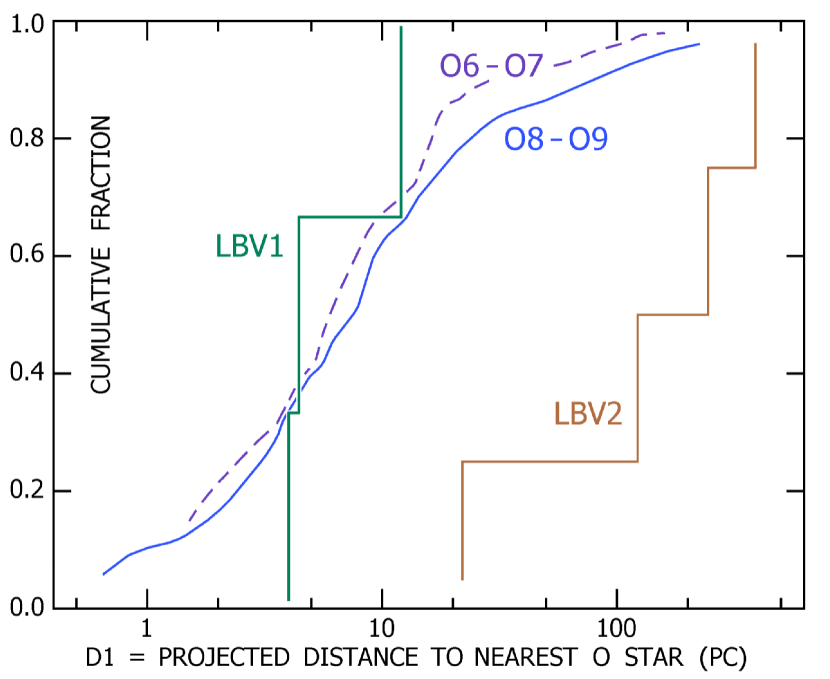
Figure 1: Distributions in the Magellanic Clouds, plotted in the style used for KS tests. Sets LBV1 and LBV2, the classical and less-luminous LBVs, were recognized long before $D1$ was evaluated for any of them (see HD94 and HWDG) .

(4) Regarding the older, less luminous LBVs, Smith belatedly states that the ST comparison sample of red supergiants must now be revised by deleting the lowest-mass members. Instead of presenting the new distribution, he conjectures that it would alter HWDG’s results.

Instead of arguing about RSG comparison samples, we can simply examine the four stars in HWDG’s “set LBV2,” the confirmed less-luminous LBVs in the Magellanic Clouds. Two of them, R71 and R110, are located more than 200 pc from their nearest known O-type stars. Does this fact imply greatly extended lifetimes? Probably not, since the expected ages of lower-luminosity LBVs appear adequate to account for it. In the standard scenario outlined by HD94 and HWDG, these objects should be more than 5 Myr old, exceeding all normal O-type stars; see Ekstrom et al (2012), Chen et al. (2015), HWDG’s Figure 1, and the 5-Myr isochrone in Fig. 12 of Martins et al (2005). Therefore, we can reasonably surmise that massive stars which formed along with R71 and R110 have now evolved beyond O9. Rotation and extra mass loss may reinforce this explanation. In order to argue that these stars require extended lifetimes in the sense that ST proposed – a strong assertion – one would need to disprove the above assessment, not merely express hypothetical reasons why it might be wrong.

(5) Smith next asserts that the standard view requires classical LBVs to be associated with O2-O5 stars, rather than later-type O stars. This claim is illogical, since LBVs are expected to be older than the O2-O5 stars. Classical LBVs should be roughly 3.5 Myr old in the standard view, while the maximum for a normal O5 star is about 2.5 Myr and, more important, the median for O2-O5 stars is less than 1.5 Myr. These estimates are based on Ekstrom et al (2012), Chen et al. (2015) with LMC metallicities, and the locations of R127 and similar stars in the HR diagram. Classical LBVs might even be older than 4 Myr if they rotate rapidly.

In Smith’s Figure 2, the O2-O5 distribution greatly differs from O6-O9 because 40% of its members have separation parameters $D1<3$ pc. Such small values indicate average ages less than 1 Myr, too young for us to expect a spatial correlation with LBVs. The O6-O9 stars provide a far more logical comparison, since many of them have ages of 3–4 Myr. In summary, his Figure 2 relates to star formation history, not LBV physics.

4 Velocities

HWDG noted that LBVs do not have the high velocities that would occur in the scenario that ST described. In order to transfer a significant amount of material, the assumed type of binary has to be close, with orbital speeds of the order of 200 km s^-1. Allowing for complications, one can reasonably expect runaway velocities well above 50 km s^-1 in at least a few cases, contrary to observations.

Smith now explains this by declaring, after lengthy preliminaries, that the required supernova occurs only after its star has been reduced to about 4 $M_{\odot}$ – so the other (future LBV) star’s orbital speed becomes less than 30 km s^-1. But he does not say why this should always be true. ST employed the word “kick” repeatedly, in a way that implied a major role for enhanced velocities. Therefore Smith’s reassessment alters their model in order to cancel a failed prediction.

His §5 recounts more KS tests, now referring to velocities in M31 and M33. They produce no significant result apart from the obvious lack of high-speed LBVs.

Then he adjusts a model of recoil speeds to optimize its KS $p$ value, and finds that it differs from the zero-extra-velocity case. But this result is inevitable because the parameter of interest is non-negative, $V_{k}\geq 0$. Even if its true value is zero, statistical errors always repel the formal best-fit value away from $V_{k}=0$ because that is the limit of the allowed range.

One particular misconception should be noted here to forestall it from propagating in the literature. Smith says that R71 “has a radial velocity that is offset by $-71$ km s^-1 relative to the systemic velocity of the LMC.” This difference is meaningless, because the star’s velocity agrees well with the rotation curve at its particular location. As HWDG carefully stated, the LMC LBV velocities are consistent “with their positions based on the H I rotation curve available at NED.”

5 AG Car and Gaia

Smith & Stassun (2016) recently noted that preliminary Gaia data appear to place AG Car only about 2 kpc from us, rather than 6 kpc as expected. Since this star is often cited as a classical LBV, they speculate that further data will lead to a revolution in this topic and a vindication of the ST scenario. That view has some obvious difficulties.

First, though, they misrepresent the state of the topic in general, by asserting that “several aspects of [the] traditional view have started to unravel.” This is a serious exaggeration. Some of the examples that they cite to support it concern superficial details rather than fundamentals, while the others have little to do with the basic LBV problem. Two of their examples – one involving $\eta$ Car, and the other repeating ST’s claims – are flatly erroneous. Smith and Stassun refrain from citing papers that disproved their arguments – e.g., Davidson & Humphreys (2012) and HWDG.

Concerning AG Car: The quoted Gaia parallax has a stated $1\sigma$ uncertainty worse than $\pm\,50$%. This is bad enough, but in addition, since it is far worse than the expected capability of the instrument, we can reasonably suspect that major systematic errors have not yet been diagnosed. Distances of classical LBVs in M31, M33, and the LMC are far more robust, and they all support the standard view (see HWDG). Given their mutual consistency, and the provisional nature of early Gaia results, it is highly imprudent to claim that $D>4$ kpc has been ruled out for AG Car.

Another objection concerns physics. The methods used to estimate $L/M$ from spectra (see refs. in §2 above) are not very sensitive to distance. If we conceptually move AG Car to $D<2.5$ kpc, then it has a truly peculiar set of attributes: (1) $L\gtrsim 10^{5}\;L_{\odot}$, but (2) $M\sim 5\;M_{\odot}$ which is amazingly small for that luminosity, while (3) it has hydrogen and (4) there’s no evident companion. Meanwhile (5) it mimicks the spectra and behavior of classical LBVs in M31, M33, and the LMC! Frankly, this combination lacks credibility unless some more concrete evidence appears.

Smith and Stassun speculate that all these items might be explained in a binary context, but their story is entirely qualitative with ambiguous choices at every juncture. In most respects it scarcely resembles the Smith & Tombleson (2015) scenario; AG Car is even said to belong to the Car OB1/OB2 association, ironic in light of ST’s “isolation” argument. Rather than offering any clear insights into the LBV phenomenon, this view makes AG Car a strange object without genuine counterparts.

Considering all the known facts, the simplest (and not very surprising) explanation is that the Gaia parallax and proper motion contain one or more systematic errors that have not yet been diagnosed at this early stage. Smith and Stassun also discuss three other objects that are not worth reviewing here. The significance of $L/M$ is emphasized below.

6 Discussion

The main value of this dispute does not concern the scenario proposed by Smith & Tombleson (2015), which is not supported by the statistical tests when careful sample sets are used. Instead, this case illustrates two or three famous but often neglected principles of scentific evidence.

First, though, concerning only LBVs, the crucial point is this: Humphreys et al. (2016) showed that bright classical LBVs are spatially correlated with O-type stars while the less luminous LBVs are not. This double fact was not previously noticed, it indicates an age difference consistent with the standard account of LBVs, and it was not expected in the ST scenario. In other words it is unforeseen evidence for the standard view. Smith (2016) later objected to many details, but did not offer any concrete reason to doubt this result.

Regarding broader principles, this case highlights the dangers of statistical formalism applied to defective samples. As illustrated in the Appendix below, the Kolmogorov-Smirnov test gives false results if the sample set is a mixture of disparate classes. ST’s sample of Magellanic “LBVs” contained at least three physically distinct classes of stars, and therefore produced illusory $p$ values. If a member of a statistical sample appears doubtful for some identifiable reason, then that member should be removed. This policy would have averted serious errors in Smith and Tombleson’s arguments.

Another fundamental principle concerns burden of proof. Here we have two competing scenarios:

• The conventional view of LBVs has been familiar since the 1980s. Essentially it consists of just one hypothesis, that the observed LBV events result from instabilities that arise when $L/M$ exceeds about half the Eddington Limit (HD94; Vink 2012; Davidson 2016). This has not been proven yet, but it is conceptually straightforward and theoretically credible, it appears consistent with existing data and with existing evolution models, and no one has identified any errors serious enough to require a major change in the concept.

• Smith & Tombleson (2015) propose a different scenario motivated by statistical arguments. It is undeniably more complicated, it has multiple free parameters, it requires many assumptions that the authors did not clearly acknowledge, and it offers no physical rationale for the LBV instability.

According to normal standards the larger burden of proof rests on Smith and Tombleson, because their model entails more hypotheses and leaves more facts unexplained. They appear to assume that a statistical failure of the standard model constitutes evidence in favor of theirs. This is illogical even if one discards the standard model, because other, simpler possibilities exist. (For instance, rapid rotation can extend the lifetime of an LBV progenitor.) Moreover, HWDG showed that the standard view does not fail the tests that ST proposed. Nevertheless, Smith (2016) attempted to shift the burden of proof onto the conventional model by demanding additional tests with new comparison sets, dynamical proof of the $L/M$ ratios, etc. None of those objections constitutes positive evidence for the mass-gaining hypothesis.

Now consider physics instead of statistics. Any viable theory of LBVs must explain three conspicuous traits.

• These objects exhibit high-mass-loss episodes, or at least expanded-radius events, with particular characteristics described in HD94 and elsewhere.

• They lie near a locus in the HR diagram, often called the LBV instability strip. However, most stars in that strip are not LBVs.

• They have $L/M\sim 0.5\,(L/M)_{\mathrm{Edd}}$, anomalously large for their locations in the HR diagram. Non-LBVs in the instability strip have larger masses and therefore smaller $L/M$.

The standard view accounts for these facts as described in HD94 and Vink (2012). Smith and Tombleson, however, did not give any clear reasons for them.

If we adapt the ST scenario by invoking the same instabilities as the standard model, then the hypothesis becomes essentially this: a star gains mass from its companion, and after that it evolves in the same way as the conventional view of LBVs.   But why is the mass exchange necessary? If LBV progenitors need extended lifetimes, rapid rotation is arguably a simpler alternative. And, as explained above and in HWDG, there is no clear evidence for substantially extended lifetimes. We suspect that the mass-gainer hypothesis will soon be revised to “maybe some LBVs” instead of ST’s “certainly all of them.”

The concept of just two classes of LBVs is very likely an idealization of the truth, because we cannot easily guess what happens in borderline cases, and, besides, rotation and other parameters surely complicate the physics. Perhaps LBVs form a continuous mass- and rotation-dependent set, and in almost every case the instability arises at the time when $L/M$ first exceeds some critical value. For the less-luminous LBVs, that occurs after a complicated series of evolutionary stages. These thoughts seem adequate to explain the instability strip, even if the truth is somewhat more complex.

There is nothing wrong with hoping that binary interactions play some interesting role in this story, but it is wrong to assume that they do. In order to replace the long-standing scenario with something very different, one needs to satisfy the classic Hume-Laplace-Truzzi-Sagan rule: extraordinary claims require extraordinary evidence.

— — — — — — — — — — — —

APPENDIX: Why the KS test needs careful sampling

Imagine two physically distinct classes of objects with some distribution parameter $x$. Suppose that both classes, A and B, have accurately known distribution functions $f_{\mathrm{A}}(x)$ and $f_{\mathrm{B}}(x)$. In Figure 2 these are plotted in the style used for a KS test. Next suppose that we are given a list of $x$-values for 24 unfamiliar objects called “type C,” also shown in the figure. Formally the KS test shows that they represent a new, intermediate class different from both A and B. The $p$ value is about 0.03 relative to B and even smaller for A.

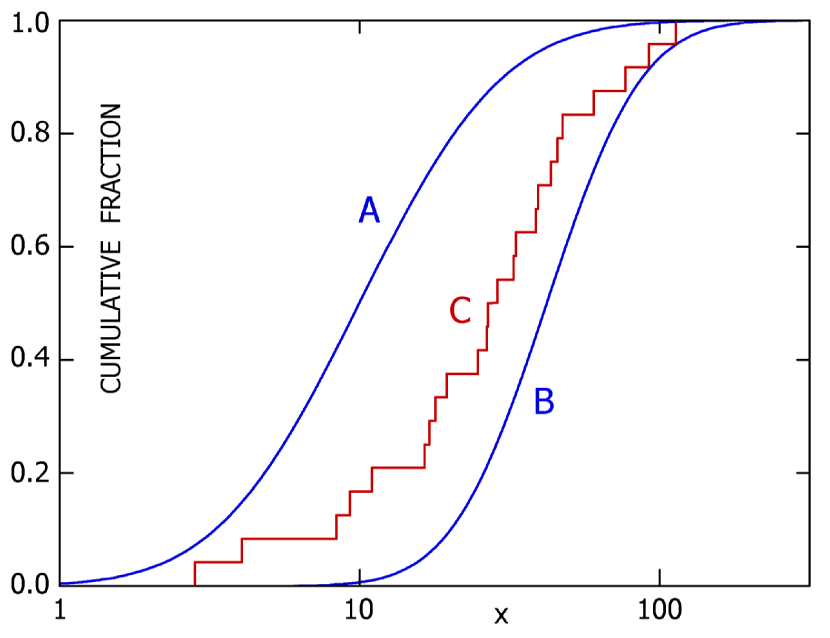
Figure 2: Distributions in a synthetic example. Set C comprises 24 objects that have not been examined closely, apart from their $x\,$-values.

However – as the reader may have guessed from the context – this conclusion is flatly wrong, because distribution C is really a mixture of 9 random A’s and 15 random B’s. (In order of increasing $x$, objects 1–5, 7, 9, 12, and 14 belong to class A.) Evidently the KS test gives meaningless results in a case like this with a mixed sample set.

This elementary example closely mirrors the test that Smith & Tombleson (2015) invoked in their §2.2. Their indirect comparison sets (O-type stars, RSGs, etc.) do not affect the issue. In the same manner as class C formally differed from both A and B in our example, Smith and Tombleson concluded that LBVs are statistically uncorrelated with particular classes of stars. (See their Figure 4.) That was incorrect because, as HWDG showed, ST’s sample set was a mixture of classical LBVs, older less-luminous LBVs, and non-LBVs. The only way to justify that KS test is to insist that their sample was acceptable despite contrary evidence.

— — —

References

- Bohannon (1989) Bohannon, B. 1989, in Physics of Luminous Blue Variables, IAU Colloq. 113, p. 35
- Chen et al. (2015) Chen, Y., Bressan, A., Girardi, L. et al. 2015, MNRAS, 452, 1068
- Conti (1984) Conti, P.S. 1984, in Observational Tests of the Stellar Evolution Theory, IAU Symp. 105, p. 233
- Davidson et al (1989) Davidson, K., Moffat, A.F.J., & Lamers, H.J.G.L.M. (eds.) 1989, Physics of Luminous Blue Variables, IAU Colloq. 113
- Davidson & Humphreys (2012) Davidson, K., & Humphreys, R.M. 2012, Nature, 486, E1
- Davidson (2016) Davidson, K. 2016, Journal of Physics Conf. Ser. 728, Issue 2, 022008; see also arXiv:1602.03925
- Ekstrom et al (2012) Ekstrom, S., et al. 2012, A&A, 537, A146
- Humphreys & Davidson (1979) Humphreys, R.M., & Davidson, K. 1979, ApJ, 232, 409
- Humphreys & Davidson (1984) Humphreys, R.M., & Davidson, K. 1984, Science, 223, 243
- Humphreys (1989) Humphreys, R.M. 1989, in Physics of Luminous Blue Variables, IAU Colloq. 113, p. 3
- Humphreys & Davidson (1994) Humphreys, R.M., & Davidson, K. 1994, PASP, 106, 1025 (“HD94”)
- Humphreys et al. (2016) Humphreys, R.M., Weis, K., Davidson, K., & Gordon, M.S. 2016, ApJ, 825:64 (“HWDG”)
- Koenigsberger et al. (2014) Koenigsberger, G., Morell, N., Hillier, D.J., et al. 2014, AJ, 148:62
- Kudritzki et al. (1989) Kudritzki, R.P., et al 1989, in Physics of Luminous Blue Variables, IAU Colloq. 113, p. 67
- Lamers (1986) Lamers, H.J.G.L.M. 1986, in Luminous Stars and Associations in Galaxies (ed. de Loore et al.), p. 157
- Lamers & de Loore (1987) Lamers, H.J.G.L.M., & de Loore, C.W.H. (eds.) 1987, Instabilities in Luminous Early Type Stars
- Martins et al (2005) Martins, F., Schaerer, D., & Hillier, D.J. 2005, A&A, 436, 1049
- Nissen et al. (2016) Nissen, S.B., Magidson, T., Gross, K., & Bergstrom, C.T. 2016, arXiv:1609.00494v1
- Pauldrach & Puls (1990) Pauldrach, A.W.W., & Puls, J. 1990, A&A, 237, 409
- Sandage & Tammann (1974) Sandage, A., & Tammann, G.A. 1974, ApJ, 191, 693
- Smith (2016) Smith, N. 2016, MNRAS, 461, 3353 (“Smith”)
- Smith & Stassun (2016) Smith, N., & Stassun, K.G. 2016, arXiv:1610.06522v1
- Smith & Tombleson (2015) Smith, N., & Tombleson, R. 2015, MNRAS, 447, 598 (“ST”)
- Stahl et al. (1990) Stahl, O., et al 1990, A&A, 228, 379
- Sterken et al. (1991) Sterken, C., et al 1991, A&A, 247, 383
- Vink (2012) Vink, J.S. 2012, in Eta Carinae and the Supernova Impostors, ASSL 384, p. 221
- Vink & de Koter (2002) Vink, J.S., & de Koter, A. 2002, A&A, 393, 543
- Wolf (1989) Wolf, B. 1989, A&A, 217, 87