Joint constraints on the Galactic dark matter halo and GC from hypervelocity stars

Abstract

The mass assembly history of the Milky Way can inform both theory of galaxy formation and the underlying cosmological model. Thus, observational constraints on the properties of both its baryonic and dark matter contents are sought. Here we show that hypervelocity stars (HVSs) can in principle provide such constraints. We model the observed velocity distribution of HVSs, produced by tidal break-up of stellar binaries caused by Sgr A*. Considering a Galactic Centre (GC) binary population consistent with that inferred in more observationally accessible regions, a fit to current HVS data with significance level $>5\%$ can only be obtained if the escape velocity from the GC to 50 kpc is $V_{\rm G}\lower 2.15277pt\hbox{$\;\buildrel<\over{\sim}\;$}850$ km s^-1, regardless of the enclosed mass distribution. When a NFW matter density profile for the dark matter halo is assumed, haloes with $V_{\rm G}\lower 2.15277pt\hbox{$\;\buildrel<\over{\sim}\;$}850$ km s^-1are in agreement with predictions in the $\Lambda$CDM model and that a subset of models around $M_{\rm 200}\sim 0.5-1.5\times 10^{12}M_{\odot}$ and $r_{\rm s}\lower 2.15277pt\hbox{$\;\buildrel<\over{\sim}\;$}35$ kpc can also reproduce Galactic circular velocity data. HVS data alone cannot currently exclude potentials with $V_{\rm G}>850$ km s^-1. Finally, specific constraints on the halo mass from HVS data are highly dependent on the assumed baryonic mass potentials. This first attempt to simultaneously constrain GC and dark halo properties is primarily hampered by the paucity and quality of data. It nevertheless demonstrates the potential of our method, that may be fully realised with the ESA Gaia mission.

1 Introduction

The visible part of galaxies is concentrated in the centre of more extended and more massive dark matter structures, that are termed haloes. In our Galaxy, the baryonic matter makes up a few percent of the total mass, and the halo is $\sim 10$ times more extended than the Galactic disc. In the current paradigm, galaxies assemble in a hierarchical fashion from smaller structures and the result is due to a combination of merger history, the underlying cosmological model and baryonic physics (e.g. cooling and star formation). Thanks to our vantage point, these fundamental ingredients in galaxy assembly, can be uniquely constrained by observations of the matter content of the Milky Way and its distribution, when analysed in synergy with dedicated cosmological simulations.

Currently, our knowledge of the Galactic dark matter halo is fragmented. Beyond $\sim 10$ kpc dynamical tracers such as halo field stars and stellar streams become rarer and rarer and astrometric errors significant. In particular, there is a large uncertainty in the matter density profile, global shape, orientation coarseness (e.g. Bullock et al., 2010; Law & Majewski, 2010; Vera-Ciro & Helmi, 2013; Loebman et al., 2014; Laevens et al., 2015; Williams & Evans, 2015) and current estimates of the halo mass differ by approximately a factor of 3 (see fig.1 in Wang et al., 2015, and references therein). This difference is significant as a mass measurement in the upper part of that range together with observations of Milky Way satellites can challenge (Klypin et al., 1999; Moore et al., 1999; Boylan-Kolchin et al., 2011) the current concordance cosmological paradigm: the so-called $\Lambda$ cold dark matter model ($\Lambda$CDM). In particular, the “too big to fail problem" (Boylan-Kolchin et al., 2011) states that, in $\Lambda$CDM high mass ($\lower 2.15277pt\hbox{$\;\buildrel>\over{\sim}\;$}2\times 10^{12}M_{\odot}$) haloes, the most massive subhaloes are too dense to correspond to any of the known satellites of the Milky Way. Therefore, the solution may simply be a lighter Galactic halo of $<10^{12}M_{\odot}$ (e.g. Vera-Ciro et al., 2013; Gibbons et al., 2014). This is an example of how a robust measurement of the Galactic mass can be instrumental to test cosmological models.

On the other extreme of Galactic scales, the Galactic Centre (GC) has been the focus of intense research since the beginning of the 1990s, and it is regarded as a unique laboratory to understand the interplay between (quiescent) supermassive black holes (SMBHs) and their environment (see Genzel et al., 2010, for a review). Indeed, the GC harbours the best observationally constrained SMBH, called Sgr A*, of mass $\approx 4.0\times 10^{6}M_{\odot}$ (Ghez et al., 2008; Gillessen et al., 2009; Meyer et al., 2012). In particular, GC observations raise issues on the stellar mass assembly, which is intimately related to the SMBH growth history. For example, in the central $r\sim 0.5$ pc the light is dominated by young ($\sim 6$ Myr old) stars (e.g. Paumard et al., 2006; Lu et al., 2013) with a suggested top-heavy initial mass function (IMF Bartko et al., 2010; Lu et al., 2013) and a large spread in metallicity at $r<1$ pc (Do et al., 2015). The existence of young stars well within the gravitational sphere of influence of Sgr A* challenges our knowledge of how stars form, as molecular clouds should not survive tidal forces there. These stars are part of a larger scale structure called nuclear star cluster with half-light radius around $\sim 5$ pc (e.g. Schödel et al., 2014b; Fritz et al., 2016): in contrast with the inner region, its IMF may be consistent with a Chabrier/Kroupa IMF and between $2.5$ pc $<r<4$ pc the majority of stars appear to be older than 5 Gyr (e.g. Pfuhl et al., 2011; Fritz et al., 2016). The origin of this nuclear star cluster and its above mentioned features is highly debated, and the leading models consider coalescence of stellar clusters that reach the GC and are tidally disrupted or in situ formation from gas streams (see Böker, 2010, for a review on nuclear star cluster). The Hubble Space Telescope imaging surveys have shown that most galaxies contain nuclear clusters in their photometric and dynamical centres (e.g. Carollo et al., 1997; Georgiev & Böker, 2014; Carson et al., 2015), but the more observationally accessible and best studied one is the Milky Way’s, which once more give us a chance of understanding the formation of galactic nuclei in general. However, to investigate the GC via direct observations, one must cope with observational challenges such as the strong and spatially highly variable interstellar extinction and stellar crowding. A concise review of the current knowledge of the nuclear star cluster at the GC and the observational obstacles and limitations is given in Schödel et al. (2014a).

Remarkably, a single class of objects can potentially address the mass content issue from the GC to the halo: hypervelocity stars (HVSs). These are detected in the outer halo (but note Zheng et al., 2014) with radial velocities exceeding the Galactic escape speed (Brown et al. 2005; see Brown, 2015, for a review). So far around 20 HVSs have been discovered with velocities in the range $\sim 300-700$ km s^-1, and trajectories consistent with coming from the GC. Because of the discovery strategy, they are all B-type stars mostly in the masses range between $2.5-4M_{\odot}$ (e.g. Brown et al., 2014). Studying HVSs is thus a complementary way to investigate the GC stellar population, by surveying more accessible parts of the sky. After ejection, HVS dynamics is set by the Galactic gravitational field. Therefore, regardless of their origin, HVS spatial and velocity distributions can in principle probe the Galactic total matter distribution (Gnedin et al., 2005, 2010; Yu & Madau, 2007; Sesana et al., 2007; Perets et al., 2009; Fragione & Loeb, 2016).

Retaining hundreds of km s^-1in the halo while originating from a deep potential well requires initial velocities in excess of several hundreds of km s^-1Kenyon et al. (2008), which are very rarely attained by stellar interaction mechanisms put forward to explain runaway stars (e.g. Blaauw, 1961; Aarseth, 1974; Eldridge et al., 2011; Perets & Šubr, 2012; Tauris, 2015; Rimoldi et al., 2016). Velocity and spatial distributions of runaway and HVSs are indeed expected to be different (Kenyon et al., 2014). For example, high velocity runaway stars would almost exclusively come from the Galactic disc (Bromley et al., 2009). Instead, HVS energetics and trajectories strongly support the view that HVSs were ejected in gravitational interactions that tap the gravitational potential of Sgr A*, and, as a consequence of a huge “kick”, escaped into the halo. In particular, most observations are consistent with the so called “Hills’ mechanism”, where a stellar binary is tidally disrupted by Sgr A*. As a consequence, a star can be ejected with a velocity up to thousands km s^-1(Hills, 1988). Another appealing feature is that the observed B-type stellar population in the inner parsec — whose in situ origin is quite unlikely — is consistent with being HVSs’ companions, left bound to Sgr A* by the Hills’ mechanism (Zhang et al., 2013; Madigan et al., 2014).

In a series of three papers, we have built up a solid and efficient semi-analytical method that fully reproduces 3-body simulation results for mass ratios between a binary star and a SMBH ($m_{\rm t}/M\sim 10^{-6}$) expected in the GC. In particular we reproduce star trajectories, energies after the encounter and ejection velocity distributions (see Sari et al., 2010; Kobayashi et al., 2012; Rossi et al., 2014, and section 2 in this paper). Here, we will capitalise on that work and apply our method to the modelling of current HVS data, with the primary aim of constraining the Galactic dark matter halo and simultaneously derive consequences for the binary population in the GC. Since star binarity is observed to be very frequent in the Galaxy (around $50\%$) and the GC seems no exception ($\sim 30\%$ for massive binaries Pfuhl et al., 2014), clues from HVS modelling are a complementary way to understand the stellar population within the inner few parsecs from Sgr A*.

This paper is organised as follows. In Section 2, we describe our method to build HVS ejection velocity distributions, based on our previous work on the Hills’ mechanism. In Section 3 , we present our first approach to predict velocity distributions in the outer Galactic halo and we show our results when comparing them to data in Section 3.3. In Section 4, we will specialise to a “Navarro, Frenk and White” (NFW) dark matter profile and present results in Section 4.2. In Section 5, we discuss our findings, their limitations and implications and then conclude. Finally, in Appendix A, we describe our analysis of the Galactic circular velocity data, that we combine with HVS constraints.

2 Ejection velocity distributions

We here present our calculation of the ejection velocity distribution of hypervelocity stars (i.e. the velocity distribution at infinity with respect to the SMBH) via the Hills’ mechanism. We denote with $M$ Sgr A*’s mass, fixed to $M=4.0\times 10^{6}M_{\odot}$.

Let us consider a stellar binary system with separation $a$, primary mass $m_{\rm p}$, secondary mass $m_{\rm s}$, mass ratio $q=m_{\rm s}/m_{\rm p}\leq 1$, total mass $m_{\rm s}+m_{\rm p}=m_{\rm t}$ and period $P$. If this binary is scattered into the tidal sphere of Sgr A*, the expectation is that its centre of mass is on a nearly parabolic orbit, as its most likely place of origin is the neighbourhood of Sgr A*’s radius of influence. Indeed, this latter is $\sim 5$ orders of magnitude larger than the tidal radius, and therefore the binary’s orbit must be almost radial to hit the tiny Sgr A*’s tidal sphere. On this orbit, the binary star has $\sim 90\%$ probability to undertake an exchange reaction, where a star remains in a binary with the black hole, while the companion is ejected. In addition, we proved that the ejection probability is independent of the stellar mass, when the centre of mass of the binary is on a parabolic orbit. This is different from the case of elliptical or hyperbolic orbits where the primary star, carrying most of the orbital energy, has a greater chance to be respectively captured or ejected. (Kobayashi et al., 2012).

The ejected star has a velocity at infinity, in solely presence of the black hole potential, equal to

$$v_{\rm ej}=\sqrt{\frac{2\,Gm_{\rm c}}{a}}\left(\frac{M}{m_{\rm t}}\right)^{1/6},$$ (1)

(Sari et al., 2010) where $m_{\rm c}$ is the mass of the binary companion star to the HVS and $G$ is the gravitational constant. Rigorously, there is a numerical factor in front of the square root in (eq. 1) that depends on the binary-black hole encounter geometry. However, this factor is $\sim 1$, when averaged over the binary’s phase. Moreover, the velocity distributions obtained with the full numerical integration of a binary’s trajectory and those obtained with (eq. 1) are almost indistinguishable (Rossi et al., 2014). Given these results and the simplicity of eq. 1, it is possible to predict ejection velocity distributions, efficiently exploring a large range of the parameter space in Galactic potentials, binary separations and stellar masses. This latter is the main advantage over methods using 3-body (or N-body) simulations.

Since we are only considering binaries with primaries’ mass $\lower 2.15277pt\hbox{$\;\buildrel>\over{\sim}\;$}3M_{\odot}$, we may consider observations of B-type and O-type binary stars for guidance. Because of the large distance and the extreme optical extinction, observations and studies of binaries in the inner GC are limited to a handful of very massive early-type binary stars (e.g. Ott et al., 1999; Pfuhl et al., 2014) and X-ray binaries (e.g. Muno et al., 2005).

For more reliable statistical inferences, we should turn to observations of more accessible regions in the Galaxy and in the Large Magellanic Cloud (LMC). They suggest that a power-law description of these distributions is reasonable. In the Solar neighbourhood, spectroscopic binaries with primary masses between $1-5M_{\odot}$ have a separation distribution, $f_{\rm a}$, that for short periods can be both approximated by a $f_{\rm a}\propto a^{-1}$ (Öpik’s law, i.e. $f(\log_{10}{P})\propto\left(\log_{10}P\right)^{\eta}$, with $\eta=0$) and a log normal distribution in period with $\left<P\right>\simeq 10$ day and a $\sigma_{\rm logP}\simeq 2.3$ (Kouwenhoven et al., 2007; Duchêne & Kraus, 2013). However, in the small separation regime, relevant for the production of HVSs, the log normal distribution may also be described by a power-law: $f_{\rm a}\propto a^{0.8}$. For primary masses $>16M_{\odot}$, Sana et al. (2012) find a relatively higher frequency of short-period binaries in Galactic young clusters, $\eta\approx-0.55$, but a combination of a pick at the smallest periods and a power-law may be necessary to encompass all available observations (see e.g. Duchêne & Kraus, 2013). For this range of massive stars ($\sim 20M_{\odot}$), a similar power-law distribution $\eta\approx-0.45$ is also consistent with a statistical description of O-type binaries in the VLT-FLAMES Tarantula Survey of the star forming region 30 Doradus of the LMC (Sana et al., 2013). In the same region, a similar analysis for observed early ($\sim 10M_{\odot}$) B-type binaries recovers instead an Öpik’s law (Dunstall et al., 2015).

Mass ratio distributions, $f_{\rm q}$, for Galactic binaries are generally observed to be rather flat, regardless of the primary’s mass range (e.g. Sana et al., 2012; Kobulnicky et al., 2014; Duchêne & Kraus, 2013, see their table 1). Differently, in the 30 Doradus star forming region, the mass ratio distributions appear to be steeper, ($f_{\rm q}\propto q^{\sim(-1)}$ in O-type banaries and $f_{\rm q}\propto q^{\sim(-3)}$ in early B-type ones), suggesting a preference for pairing with lower-mass companions: still a power-law may be fitted to data (Sana et al., 2013; Dunstall et al., 2015).

We therefore assume a binary separation distribution

$$f_{\rm a}\propto a^{\alpha},$$ (2)

where the minimum separation is taken to be the Roche-Lobe radius $a_{\rm min}=2.5\times\max[R_{*},R_{\rm c}]$, where $R_{*}$ and $R_{\rm c}$ are the HVS’s and the companion’s radii, respectively. As a binary mass ratio distribution, we assume

$$f_{\rm q}\propto q^{\gamma},$$ (3)

for $m_{\rm min}\leq m_{\rm s}\leq m_{\rm p}$. If not otherwise stated, $m_{\rm min}=0.1M_{\sun}$.

The mass of the primary star ($m_{\rm p}\gtrsim 3M_{\odot}$) is taken from an initial mass function, that needs to mirror the star formation in the GC in the last $\sim 10^{9}$ yr. As mentioned in our introduction, the stellar mass function is rather uncertain and may be spatially dependent. Observations of stars with $M>10M_{\odot}$ within about $0.5$ pc from Sgr A* indicate a rather top-heavy mass function with $f_{\rm m}\propto m_{\rm p}^{-1.7}$ (Lu et al., 2013). At larger radii observations of red giants (and the lack of wealth of massive stars observed closer in) may instead point towards a more canonical bottom-heavy mass function (e.g. Pfuhl et al., 2011; Fritz et al., 2016). Given these uncertainties, we explore the consequences of assuming either a Kroupa mass function (Kroupa, 2002), $f_{\rm m}\propto m_{\rm p}^{-2.3}$ or top-heavy distribution, $f_{\rm m}\propto m_{\rm p}^{-1.7}$, in the mass range $2.5M_{\odot}\leq m_{\rm p}\leq 100M_{\odot}$.

Finally, we do not introduce here any specific model for the injection of binaries in the black hole tidal sphere and consequently, we do not explicitly consider any “filter" or modification to the binary “natal” distributions. Likewise, we do not explicitly account for higher order multiplicity (e.g. binary with a third companion, i.e. triples) that may result in disruption of binaries with different distributions than those cited above. On the other hand, a way to interpret our results is to consider that the separation and mass ratio distributions already contain those modifications. We will explore these possibilities in Section 5.

3 Predicting velocity distributions in the halo: first approach.

In this Section, we first describe how we compute the halo velocity distribution with a method that allows us to use a single parameter to describe the Galactic deceleration, without specifying its matter profile (Sec. 3.1) . Given the large Galactocentric distances at which the current sample of HVSs is observed, our method is shown to be able to reproduce the correct velocity distribution for the velocity range of interest, without the need to calculate the HVS deceleration along the star’s entire path from the GC. These features allow us to efficiently explore a large range of the binary population and the dark matter halo parameter space. Then, in Sec. 3.2, we describe how we perform our comparison with current selected data and finally we present our results in Sec. 3.3.

3.1 Velocity distribution in the halo: global description of the potential

Our first approach follows Rossi et al. (2014) and consists in not assuming any specific model for the Galactic potential, but rather to globally describe it by the minimum velocity, $V_{\rm G}$, that an object must have at the GC in order to reach 50 kpc with a velocity equal or greater than zero. In other words, the parameter $V_{\rm G}~{}$is a measure of the net deceleration suffered by a star ejected at the GC into the outer halo, regardless of the mass distribution interior to it. The statement is that Galactic potentials with the same $V_{\rm G}~{}$produce the same velocity distribution beyond 50 kpc, which is where most HVSs are currently observed.

The physical argument that supports this statement is the following. For any reasonable distribution of mass that accounts for the presence of the observed bulge, most of the deceleration occurs well before stars reach the inner halo (e.g. Kenyon et al., 2008) and therefore, any potential with the same escape velocity $V_{\rm G}~{}$will have the same net effect on an initial ejection velocity:

$$v=\sqrt{v_{\rm ej}^{2}-V_{\rm G}^{2}}.$$ (4)

Although practically we are interested in the HVS distribution beyond $50$ kpc, the method outlined here is valid for any threshold distance as long as the deceleration beyond that is negligible and, as justified below, all stars in the velocity range of interest reach it within their life-time. Therefore in the following, when a specific choice is not needed, we will generically call this threshold distance “$r_{\rm in}$". This, we recall, is also the radius associated to $V_{\rm G}~{}$.

Let us now proceed to calculate the HVS velocity distribution within a given radial range $\Delta r=[r_{\rm out}-r_{\rm in}]$ in spherical symmetry, assuming a time-independent ejection rate $\cal{R}$ (typically $\sim 10-100$ Myr^-1). Given the above premises, HVSs with a velocity around $v$ cross $r_{\rm in}$ at a rate $d\dot{N}/dv$, that can be obtained from the ejection-velocity probability density function (PDF) $P(v_{\rm ej})$ equating bins of corresponding velocity,

$$\frac{d\dot{N}}{dv}dv={\cal R}P(v_{\rm ej}){\rm d}v_{\rm ej},$$

with the aid of eq.4, that gives $v=v(v_{\rm ej})$. Consequently, the halo-velocity PDF ($dn/dv$) within a given radial range $\Delta r$ can be simply computed as

$$dn(v,\Delta r)\propto\frac{d\dot{N}}{dv}\times\min[\Delta r/v,\left<t_{\rm life}\right>]\,dv,$$ (5)

where $\min[\Delta r/v,\left<t_{\rm life}\right>]$ is the average residence time in that range of Galactocentric distances of HVSs in a bin $dv$ of velocity around $v$. This is the minimum between the crossing time $\Delta r/v$ and the average life-time $\left<t_{\rm life}\right>$ beyond $r_{\rm in}$ of a star in that velocity bin. This latter term accounts for the possibility that stars may evolve out of the main sequence and meet their final stellar stages before they reach the maximum radial distance considered (i.e. $r_{\rm out}$) .

More precisely for a given star $t_{\rm life}$ should be equal to the time left from its main sequence lifetime $t_{\rm MS}$, after it has dwelled for a time $t_{\rm ej}$ in the GC, and subsequently travelled to $r_{\rm in}$ in a flight-time $\tau(r_{\rm in})$: $t_{\rm life}=t_{\rm MS}-(t_{\rm ej}+\tau(r_{\rm in}))$. Observations suggest that a HVS can be ejected at anytime during its lifetime with equal probability and therefore on average $t_{\rm ej}\approx t_{\rm MS}/2$ (Brown et al., 2014). In addition, if $\tau(r_{\rm in})\ll t_{\rm MS}$, we can write $\left<t_{\rm life}\right>=\left<t_{\rm MS}\right>/2$, where $\left<t_{\rm MS}\right>=\int(dn/dm)~{}t_{\rm MS}(m)dm$ is the average main sequence life-time weighted for the star mass distribution $dn/dm$ in a given velocity bin.

In the HVS mass and metallicity range considered here $t_{\rm MS}(m)\approx 200-700$ Myr (and $\left<t_{\rm MS}\right>\approx 300-600$ Myr). Consequently our calculations typically show $\tau(r_{\rm in})<t_{\rm MS}$ for velocities $>150$ km s^-1, when adopting $r_{\rm in}=50$ kpc. This means that $\tau(r_{\rm in})\ll t_{\rm MS}$ in the whole velocity range of interest in this work ($v\geq 275$ km s^-1, see Section 3.2).

In this framework, we construct a Monte Carlo code where $10^{7}$ binaries are drawn from the distributions described in Section 2 to build an ejection velocity PDF. This is used to construct the expected PDF in the outer halo (eq.5) between $r_{\rm in}=50$ kpc and $r_{\rm out}=120$ kpc (the observed radial range), using the formalism detailed above. For each bin of velocity, we calculate the $\left<t_{\rm MS}\right>$, using the analytical formula by Hurley et al. (2000, see their equation 5). The lifetime for a star in the $2.3-4M_{\odot}$ range is of a few to several hundred million years, but the exact value depends on metallicity (higher metallicities correspond to longer lifetimes). Until recently, solar metallicity was thought to be the typical value for the GC stellar population. However, more recent works suggest that there is a wider spread in metallicity, with a hint for a super-solar mean value (Do et al., 2015).

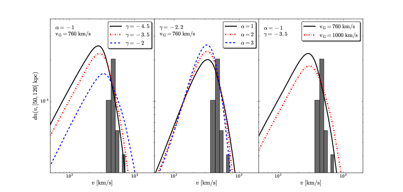
Figure 1: Probability density functions for HVS velocities in the outer halo of our Galaxy, between 50 kpc and 120 kpc. They are calculated following the deceleration procedure explained in Section 3 and depend on 3 main parameters: $\gamma$, $\alpha$ (for the binary mass ratio and semi-major axis distributions) and $V_{\rm G}~{}$. In each panel, two parameters are kept fixed while we show how the distribution changes by changing the value of the third parameter. See text for a detailed description. For a visual comparison, we over-plot data from Brown et al. (2014) (“unbound sample” only), with an arbitrary binning.

In the following, our fiducial model will assume:

• HVSs masses between 2.5 and 4 solar masses;

• A Kroupa ($f_{\rm m}\propto m_{\rm p}^{-2.3}$) IMF for primary stars between 2.5 and 100 solar masses;

• For a given primary mass $m_{\rm p}$, a mass ratio distribution $f_{\rm q}\propto q^{\gamma}$ in the range $[m_{\rm min}/m_{\rm p},1]$, with $m_{\rm min}=0.1M_{\odot}$ and $-10\leq\gamma\leq 10$;

• A separation distribution $f_{\rm a}\propto a^{\alpha}$ between $a_{\rm min}=2.5\times\max[R_{*},R_{\rm c}]$ and $a_{\rm max}=10^{3}R_{\odot}$, with $-10\leq\alpha\leq 10$;

• A HVS mean metallicity value of $Z=0.05$ (i.e. super-solar).

We will explore different assumptions in Section 5. In particular, we will investigate a top-heavy primary IMF, explore the consequence of a solar metallicity and finally assume a higher value of $m_{\rm min}$, over which we have no observational constraints in the GC. We will find that only the latter, if physically possible, may significantly impact our results and will discuss the consequences.

Examples of velocity distributions in the halo for our fiducial model are shown in Figure 1. Our selected data (see the Figure’s caption and next Section) are over-plotted with an arbitrary binning (histogram). It is here worth reminding some of the features derived in Rossi et al. (2014). There, we analytically and numerically showed that the HVS halo velocity distribution encodes different physical information in different parts of the distribution. In particular, the peak of the distribution depends on both $V_{\rm G}~{}$and the binary distributions, and moves towards lower velocity for lower $V_{\rm G}~{}$(right panel) and higher values of $|\gamma|$ and $\alpha$ (left and central panels). On the other hand, the high-velocity branch only depends on the binary properties, as the Galactic deceleration is negligible at those velocities. From eq.5, one can derive that for $v\gg v_{\rm G}$ the high-velocity branch is independent of the binary semi-major axis distribution (i.e. $\alpha$) for $\gamma>-(\alpha+2)$ and

$$dn\propto v^{2\gamma}dv.$$

Therefore larger value of $|\gamma|$ result in a steeper distribution at high velocities. This is shown in the left panel of Figure 1. Instead in the $v\gg v_{\rm G}$ and $\gamma<-(\alpha+2)$ regime,

$$dn\propto v^{-2(\alpha+2)}dv,$$

independently of the assumed mass ratio distribution and a steeper power-law is obtained for larger $\alpha$ values (central panel). A discussion on the low-velocity tail, that it is solely shaped by the deceleration, is postponed to Section 4.1.

3.2 Comparison with data

Beside the current HVS sample of so-called “unbound” HVSs (velocity in the standard rest frame $\lower 2.15277pt\hbox{$\;\buildrel>\over{\sim}\;$}275$ km s^-1), there is an equal number of lower velocity “bound” HVSs. Currently, it is unclear if they all share the same origin as the unbound sample, as a large contamination from halo stars cannot be excluded. We will therefore restrict our statistical comparison with data to the unbound sample (see upper part of table 1in Brown et al., 2014). As mentioned earlier, we only select HVS with masses between $2.5-4M_{\odot}$, with Galactocentric distances between 50 kpc and 120 kpc, for a total of 21 stars. These selections in velocity, mass and distance will be also applied to our predicted distributions.

Specifically, we calculate the total PDF as described by eq. 5 and we perform a one dimensional Kolmogorov-Smirnov (K-S) test applied to a left-truncated data sample. If we call $n(<v,\Delta r)$ the cumulative probability function (CPF) for HVS velocities in the distance range $\Delta r$, then the actual CPF that should be compared with data is,

$$n^{*}(<v,\Delta r)=\frac{n(<v,\Delta r)-n(<275~{}{\rm km~{}s^{-1}},\Delta r)}{1-n(<275~{}{\rm km~{}s^{-1}},\Delta r)}.$$ (6)

Therefore, the K-S test result is computed as

$$D\equiv\max[|n^{*}(<v,\Delta r)-n_{\rm d}(<v)|],$$ (7)

where $n_{\rm d}(<v)$ is the CPF of the actual data The significance level $\bar{\alpha}=1-P(D\leq\bar{d})$ is the probability of rejecting a fitted distribution $n(<v,\Delta r)$, when in fact it is a good fit. The most commonly used threshold levels for an acceptable fit are $\bar{\alpha}=0.01$ and $\bar{\alpha}=0.05$. For 21 data points $\bar{d}=0.344$ and $\bar{d}=0.287$ are the critical values below which the null hypothesis that the data are drawn from the model cannot be rejected at a significance level of 1% and 5% respectively.

Note that no HVS is observed with a velocity in excess of $v>700$ km s^-1. Since the HVS discovery method is spectroscopic as opposed to astrometric, there is no obvious observational bias that would have prevented us from observing HVS with $v>700$ km s^-1within 120 kpc and so we do not perform any high-velocity cut to our model. Indeed, the absence of high-velocity HVSs in the current (small) sample suggests that they are rare, and this fact puts strong constraints on the model parameters. From the discussion in the previous section, a suppression of the high-velocity branch can be achieved by either choose a lower $V_{\rm G}~{}$or choose steeper binary distributions (a larger $|\gamma|$ or $\alpha$), as we will explicitly show in the next section.

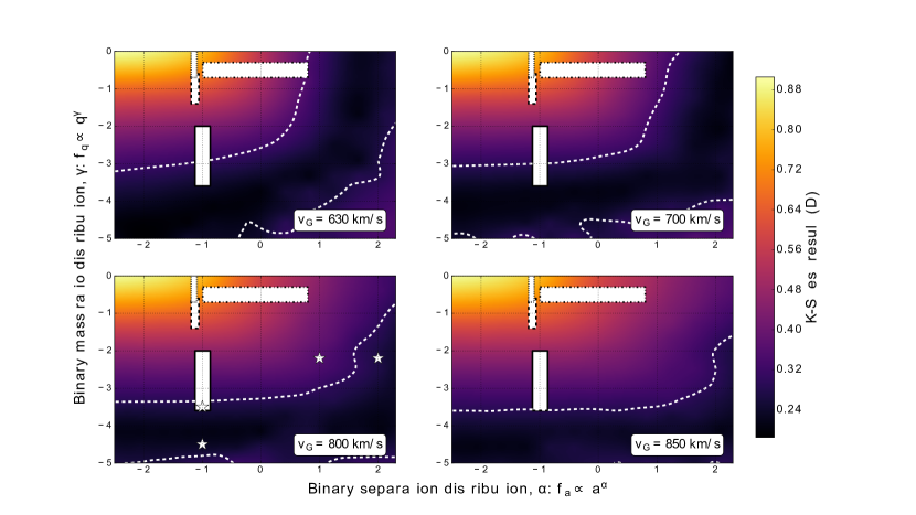
Figure 2: Contour plots for K-S test results in the parameter space $\alpha-\gamma$ for 4 different values of $V_{\rm G}$ (see panels’ label). The white dashed line indicates the $5\%$ significance level contours. The white regions correspond to observed properties of B-type or O-type binaries: the region enclosed by a dash-dotted line is for late B-type stars ($2-5M_{\odot}$) in the Solar Neighbourhood (Kouwenhoven et al., 2007; Duchêne & Kraus, 2013); results for Galactic O-type binaries are shown within the region marked by a dotted line (Sana et al., 2012); the region enclosed by a solid (dashed) line is for early $\sim 10M_{\odot}$ B-type (O-type) binaries observed in 30 Doradus (Sana et al., 2013; Dunstall et al., 2015). The four stars mark the points ($\alpha,\gamma$) in the parameter space for which the PDF is shown in Figure 1 (see also Fig.6).

3.3 Results

In each panel of Figure 2, we explore the parameter space $\alpha-\gamma$ for a fixed global deceleration that brakes stars while travelling to 50 kpc, i.e. for a given $V_{\rm G}$. The contour plots show our K-S test results and models below and at the right of the white dashed line have a significance level higher than 5%: i.e. around and below that line current data are consistent with coming from models with those sets of parameters.

Let us first focus on the upper right panel ($V_{\rm G}\approx 700$ km s^-1), as it shows clearly a common feature of all our contour plots in this parameter space. There is a stripe of minima that, from left to right, first runs parallel to the $\alpha$-axis and then to the $\gamma$-axis. This stripe is the locus of points where the high-velocity tail of the distributions has a similar slope: this happens for values of $\gamma$ and $\alpha$ related by $\gamma\approx-(\alpha+2)$ (see discussion of Figure 1 in Section 3.1). For negative $\alpha$ values (distributions with more tight binaries than wide ones), the high-velocity distribution branch is mainly shaped by the mass ratio distribution and, for example in this panel, a value around $\gamma\approx-4$ gives the best fit. On the other hand, for positive $\alpha$ (i.e. more wider binaries than tight ones), the high-velocity tail is shaped by the separation distribution and a value of around $\alpha\approx 2$ gives the best K-S results.

When increasing the escape velocity (from top left to bottom right) the stripe of minima moves towards the right lower part of the plots and gets further and further from the regions in the $\alpha-\gamma$ parameter space that correspond to observations of B-type binaries, and actually, to our knowledge, of any type of binaries currently observed with enough statistics in both star-forming and quiescent regions. We focus on observations of B-type binaries because, although our calculation consider $\sim 3M_{\odot}$ HVSs ejected from binaries with all possible mass combinations, we find that the overall velocity distribution is highly dominated by binaries where HVSs were the primary (more massive) stars, i.e. late B-type binaries.

In all panels, but the bottom right one, the white dashed line crosses or grazes the $\alpha-\gamma$ parameter space indicated by a white rectangle within a solid black line. We conclude that within an approximate range $V_{\rm G}\lower 2.15277pt\hbox{$\;\buildrel<\over{\sim}\;$}850$ km s^-1, the current observed HVS velocity distribution can be explained assuming a binary statistical description in the GC that is consistent with the one inferred by Dunstall et al. (2015) for $\sim 10M_{\odot}$ B-type binaries in the star forming region of the Tarantula Nebula. In addition, for $V_{\rm G}\lower 2.15277pt\hbox{$\;\buildrel<\over{\sim}\;$}630$ km s^-1the 5% confidence line also crosses the parameter space observed for Galactic B-type binaries (Kouwenhoven et al., 2007). An argument in favour of a similarity between known star forming regions and the inner GC is that, in this latter, Pfuhl et al. (2014) infer a binary fraction close to that in known young clusters of comparable age. However, we warn the reader that the Tarantula Nebula’s results are affected by uncertainties beyond those represented by the nominal errors on $\alpha$ and $\gamma$ reported by Dunstall et al. (2015) and we will discuss those in Section 5.

Finally, we comment on our choice to define the $V_{\rm G}~{}$limit using a 5% significance level threshold. If we relax this assumption and accept models with significance level $>1\%$ (another commonly used threshold) the $V_{\rm G}~{}$limit moves up to $V_{\rm G}\approx 930$ km s^-1. On the other hand, models with $>10\%$ significance level have $V_{\rm G}\lower 2.15277pt\hbox{$\;\buildrel<\over{\sim}\;$}800$ km s^-1. Therefore, as a representative value, we cite here and thereafter the intermediate one of $850$ km s^-1, corresponding to the 5% threshold.

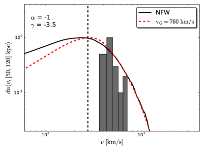
Figure 3: Galactic halo velocity distributions between 50 and 120 kpc for a fixed binary statistical description (see parameters in the upper left corner) but with different treatments of the star deceleration: the red dashed line is computed as described in Section 3.1 for $V_{\rm G}=760$ km s^-1while the black solid line is our model where stars are continuously decelerated in a potential whose halo is described by a NFW profile with mass $M_{\rm h}=0.5\times 10^{12}M_{\odot}$ and scale radius $r_{\rm s}=31$ kpc (see Section 4). This potential requires an initial velocity to escape from the GC to 50 kpc of $V_{\rm G}\approx 760$ km s^-1(see eq. 12). Unlike Figure 1, both model distributions and data are normalised at the peak for an easier visual comparison. The vertical dashed line marks the selection threshold ($v=275$ km s^-1) of the Brown et al. unbound sample. This comparison shows that for $v\lower 2.15277pt\hbox{$\;\buildrel>\over{\sim}\;$}250$ km s^-1the two distributions are similar, as confirmed by the results from the K-S test ($D=0.25$ for the black solid line and $D=0.26$ for the red dashed line).

4 Second approach: assuming a Galactic Potential model

We now choose a specific model to describe the Galactic potential, in order to cast our results in terms of dark matter mass and its spatial distribution.

We represent the dark matter halo of our Galaxy with a Navarro Frank and White (NFW) profile,

$$\phi(r)_{\rm NFW}=-GM_{\rm h}\left(\frac{\ln(1+r/r_{\rm s})}{r}\right),$$ (8)

(Navarro et al., 1996). In this spherical representation there are only two parameters: the halo mass $M_{\rm h}$ and the scale radius $r_{\rm s}$, where the radial dependence changes. Eq.8 assumes an infinite potential (no outer radius truncation) which is justified in our case since we consider Galactocentric distances smaller than the halo virial radius ($\sim 200$ kpc).

The baryonic mass components of the Galactic potential can be described by a Hernquist’s spheroid for the bulge (Hernquist, 1990),

$$\phi(r)_{\rm b}=-\frac{GM_{\rm b}}{r+r_{\rm b}},$$ (9)

(in spherical coordinates) plus a Miyamoto-Nagai disc (Miyamoto & Nagai, 1975, in cylindrical coordinates, where $r^{2}=R^{2}+z^{2}$),

$$\phi_{\rm d}(R,z)=-\frac{GM_{\rm d}}{\sqrt{R^{2}+\left(a+\sqrt{z^{2}+b^{2}}\right)^{2}}},$$ (10)

with the following parameters: $M_{\rm b}=3.4\times 10^{10}M_{\odot}$, $r_{\rm b}=0.7$ kpc, $M_{\rm d}=1.0\times 10^{11}M_{\odot}$, $a=6.5$ kpc and $b=0.26$ kpc. This Galactic model have been used in modelling both HVSs and stellar streams (e.g. Johnston et al., 1995; Price-Whelan et al., 2014; Hawkins et al., 2015, and with slightly different parameters by Kenyon et al. 2008). Observationally, our choice for the bulge’s mass profile is supported by the fact that its density profile is very similar to that obtained by Kafle et al. (2014), fitting kinematic data of halo stars in SEGUE. In addition Kafle et al. (2014) use our same model for the disc mass distribution and their best fitting parameters are very similar to our parameters (see their table 1 and 2). However, different choices may also be consistent with current data, and we will discuss the impact of different baryonic potentials on our results in Section 4.2.

In a potential constituted by the sum of all Galactic components,

$$\phi_{\rm T}(r,M_{\rm h},r_{\rm s})=\phi(r(R,z))_{\rm d}+\phi(r)_{\rm b}+\phi(r)_{\rm NFW}\,,$$ (11)

we integrate each star’s trajectory from an inner radius $r_{\rm start}=3$ pc, equal to Sgr A*’s sphere of influence but any starting radius $r_{\rm start}<20$ pc gives very similar results. In fact, we find that the disc’s sky-averaged deceleration is overall negligible with respect to that due to the bulge. To save computational time, we therefore set $R=z=r/\sqrt{2}$ in equation 10 (i.e. we only consider trajectories with a Galactic latitude of 45^∘), simplifying our calculations to one-dimensional (the Galactocentric distance $r$) solutions.

The star’s initial velocity is drawn from the ejection velocity distribution, constructed as detailed in Section 2. Assumptions on HVS properties are those of our fiducial model. Informed by observations (Brown et al., 2014), we assigned a flight-time from a flat distribution between $[0,t_{\rm MS}]$. Each integration of $10^{7}$ star orbits gives a sky realisation of the velocity PDF, but we actually find that the number of stars we are tracking is sufficiently high that differences between PDFs associated to different realisations are negligible.

An example of a halo velocity distribution is shown in Figure 3 with a black solid line. This accurate calculation of the star deceleration is well approximated by using eq.4 for $v\lower 2.15277pt\hbox{$\;\buildrel>\over{\sim}\;$}250$ km s^-1, when the escape velocity at 50 kpc is calculated as

$$V_{\rm G}^{2}=2(\phi_{\rm T}\left(50~{}{\rm kpc},M_{\rm h},r_{\rm s})-\phi_{\rm T}(r_{\rm start},M_{\rm h},r_{\rm s})\right),$$ (12)

(red dashed line in Figure 3). Despite the discrepancy in the behaviour of the low velocity tail, the two approaches give very similar K-S test results when compared to current observations ($D=0.26$ for the NFW model versus $D=0.25$ for the “$V_{\rm G}~{}$” model). With a random sampling, we tested that K-S results differ at most at percentage level in the whole extent of the parameter space of interest to us, validating our first approach, as an efficient and reliable exploratory method.

4.1 The low-velocity tail

We here pause to discuss and explain the difference in the velocity distribution around and below the peak calculated with our two approaches (see Figure 3). Without loss of indispensable information, the impatient reader may skip this section and proceed to the next one, where we discuss our results.

The low velocity tail discrepancy is due to our two main assumptions of our first method: i) neglecting the residual deceleration beyond $50$ kpc; and ii) all stars reach $50$ kpc before they evolve out of the main sequence. The residual deceleration gives an excess of low velocity stars in the correct distribution (black solid line) that cannot be reproduced by our approximated calculation (red dashed line). On the other hand, a fraction of stars that should have ended up with velocities $\lower 2.15277pt\hbox{$\;\buildrel<\over{\sim}\;$}150$ km s^-1beyond $50$ kpc have in fact flight-times longer than their life-time and the low velocity excess is slightly suppressed in that range.

Let us be more quantitative. In the framework of our first approach, one can show that the PDF at low velocities increases linearly with $v$ (Rossi et al., 2014). The calculation is as follows. The rate of HVSs crossing $r=r_{\rm in}$ with $v=\sqrt{v_{\rm ej}^{2}-V_{\rm G}^{2}}\ll V_{\rm G}$ is given by

$$\frac{d\dot{N}}{dv}\sim{\cal{R}}\left.P(v_{\rm ej})\right|_{v_{\rm ej}=V_{\rm G}}\frac{v}{V_{\rm G}}.$$

Moreover, for

$$v<\Delta r/\left<t_{\rm MS}\right>\approx 230~{}{\rm km~{}s}^{-1}(\Delta r/70\rm kpc)(300/~{}\rm Myr/\left<t_{\rm MS}\right>),$$

the residence time within $\Delta r$ is equal to (half of) the stars’ life-time, therefore from eq.5 we conclude that

$$\frac{dn(v,\Delta r)}{dv}\propto\left.P(v_{\rm ej})\right|_{v_{\rm ej}=V_{\rm G}}v\times\left<t_{\rm MS}\right>,$$

recovering the linear dependence on $v$. In fact, $\left<t_{\rm MS}\right>$ is not completely independent of $v$ as it varies by a factor of $\approx 1.5$ as $v\rightarrow 0$. Therefore $dn/dv$ is slightly sub-linear in $v$. The dependence of $\left<t_{\rm MS}\right>$ on $v$ comes about because $v_{\rm ej}$ is proportional to $m_{\rm c}$. This causes low-velocity HVSs to be increasingly of lower masses $(\rightarrow 2.5M_{\odot})$, being ejected from binaries where their companions were all lighter $m_{\rm c}\lower 2.15277pt\hbox{$\;\buildrel<\over{\sim}\;$}2.5M_{\odot}$ than the companions of more massive HVSs.

When considering instead the full deceleration of stars in a gravitational potential $a=-d\phi_{\rm T}(r)/dr$ as they travel towards $r_{\rm out}$, their velocity depends both on $v_{\rm ej}$ and $r$,

$$v(v_{\rm ej},r)=\sqrt{v_{\rm ej}^{2}-\left(V_{\rm esc}(0)^{2}-V_{\rm esc}(r)^{2}\right)},$$ (13)

where $V_{\rm esc}(r)$ is the escape velocity from a position r to infinity (i.e. $V_{\rm esc}(0)$ is the escape velocity from the GC to infinity). Note that $V_{\rm G}=\sqrt{V_{\rm esc}(0)^{2}-V_{\rm esc}(r_{\rm in})^{2}}$. In the example shown in Figure 3, $V_{\rm esc}(0)\approx 826$ km s^-1, $V_{\rm esc}(r_{\rm in}=50~{}\rm kpc)\approx 323$ km s^-1, $V_{\rm esc}(r_{\rm out}=120~{}\rm kpc)\approx 257$ km s^-1and $V_{\rm G}\approx 760$ km s^-1. On the other hand, the distance $r$ is a function of both $v_{\rm ej}$ and the flight-time $\tau(r)=\int dv(r)/\left|a(r)\right|$, and this latter is a preferable independent variable because uniformly distributed. Therefore we express $v=v(v_{\rm ej},\tau)$ and

$$\frac{dn}{dv}\propto\int_{0}^{\left<t_{\rm MS}\right>}\int_{v_{\rm ej,min}}^{v_{\rm ej,max}}\delta{(v-v(v_{\rm ej},\tau))}P(v_{\rm ej})dv_{\rm ej}d\tau,$$ (14)

where the relevant ejection velocity range is that that gives low-velocity stars between $r_{\rm in}$ and $r_{\rm out}$: $v_{\rm ej,min}=\sqrt{v^{2}+\left(V_{\rm esc}(0)^{2}-V_{\rm esc}(r_{\rm in})^{2}\right)}$ and $v_{\rm ej,max}=\sqrt{v^{2}+\left(V_{\rm esc}(0)^{2}-V_{\rm esc}(r_{\rm out})^{2}\right)}$. Note that, for Galactic mass distribution where $V_{\rm esc}(0)>V_{\rm esc}(r_{\rm in}),V_{\rm esc}(r_{\rm out})$, the range $[v_{\rm ej,min}-v_{\rm ej,max}]$ is rather narrow and for $v\ll V_{\rm G}$ these limits may be taken as independent of $v$. This is the case in the example of Fig. 3, where $v_{\rm ej,min}\approx V_{\rm G}\approx 760<v_{\rm ej}[\rm km~{}s^{-1}]<v_{\rm ej,max}\approx 785$.

It follows that the low-velocity tail is populated by stars that where ejected with velocities slightly higher than $V_{\rm G}$. If we further assume that the flight-time $\tau$ to reach any radius within $r_{\rm out}$ is always smaller than $\left<t_{\rm MS}\right>$ (formally this means putting the upper integration limit in $\tau$ equal to infinity), then all HVSs ejected with that velocity reach 50 kpc. It may be therefore intuitive that, applying the above considerations, eq.14 reduces to

$$\frac{dn}{dv}(v,\Delta r)\propto\left.P(v_{\rm ej})\right|_{v_{\rm ej}=V_{\rm G}}\int_{r_{\rm in}}^{r_{\rm out}}\frac{dr}{v_{\rm ej}(r)}\approx\left.P(v_{\rm ej})\right|_{v_{\rm ej}=V_{\rm G}}\frac{\Delta r}{V_{\rm G}},$$ (15)

where we substitute $d\tau=dv/|a|$ in eq.14 and we use eq.13. We therefore recover the flat behaviour for $v\lower 2.15277pt\hbox{$\;\buildrel<\over{\sim}\;$}300$ km s^-1of the black solid line in Figure 3. We, however, also notice that below $\sim 150$ km s^-1there is a deviation from a flat distribution: this is because our assumption of $\tau(r_{\rm in})\ll\left<t_{\rm MS}\right>$ breaks down, as not all stars reach $50$ kpc, causing a dearth of HVSs in that range.

As a concluding remark, we stress that, although we do not apply it here, the result stated in eq.15 can be used to further improve our first method, a necessity when low-velocity data will be available.

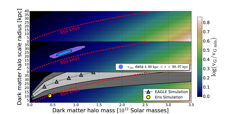
Figure 4: Upper panel: the “escape" velocity from the GC to $50$ kpc, $V_{\rm G}$, over the minimum allowed by the presence of a baryonic disc and bulge ($V_{\rm G,min}=725$ km s^-1) is mapped onto the $M_{\rm h}-r_{\rm s}$ parameter space for NFW dark halo profiles using eq. 12. The iso-contour line equal to $V_{\rm G}=850$ km s^-1is explicitly marked as red dashed line. Middle panel: same as the upper panel but over-plotted are the results of our MCMC analysis of the Galactic circular velocity data from Huang et al. (2016) (see Appendix A). Lower panel: the same as the upper panel but over-plotted are results from the Eris (Guedes et al., 2011) and EAGLE (Schaye et al., 2015) simulations. These are dark matter plus baryons simulations: the first one is a single realisation of a Milky Way-type galaxy, the latter are cosmological simulations that span a wider range of masses $(10^{10}-10^{14}M_{\odot})$. Following Schaller et al. (2015), figure 11 middle panel, we plot the mass concentration relation found in EAGLE in our mass range, with a scatter in the concentration parameter of $25\%$ at one sigma level.

4.2 Results

The relation given by eq. 12 allows us to map a given $V_{\rm G}$ value onto the $M_{\rm h}-r_{\rm s}$ parameter space. This is shown in Figure 4, upper panel. Note that for a given choice of the baryonic mass components of the potential, there is an absolute minimum for $V_{\rm G}$ (thereafter $V_{\rm G,min}$) , that corresponds to the absence of dark matter within 50 kpc. For our assumptions (eqs. 9 and 10), $V_{\rm G,min}\approx 725$ km s^-1. In other words, this is the escape velocity from the GC only due to the deceleration imparted by the mass in the disc and bulge components.

In Figure 4, the red dashed curve marks the iso-contour equal to $V_{\rm G}=850$ km s^-1: above this curve $V_{\rm G,min}\lower 2.15277pt\hbox{$\;\buildrel<\over{\sim}\;$}V_{\rm G}<850$ km s^-1. For a scale radius of $r_{\rm s}<30$ kpc, this region corresponds to $M_{\rm h}<1.5\times 10^{12}M_{\odot}$, but, if larger $r_{\rm s}~{}$can be considered, the Milky Way mass can be larger. This parameter degeneracy is the result of fitting a measurement that — as far as deceleration is concerned — solely depends on the shape of the potential within 50 kpc: lighter, more concentrated haloes give the same net deceleration as more massive but less concentrated haloes. The $V_{\rm G}=850$ km s^-1line stands as an indicative limit above which, for a given halo mass, HVS data can be fitted at $>5\%$ significance level assuming a B-type binary population in the GC close to that inferred in the LMC. In fact, since in our case $V_{\rm G,min}>630$ km s^-1, the observed Galactic binary statistics never gives a high significance level fit to current data (see Section 3.3).

To gain further insight into the likelihood of various regions of the parameter space, we compare our results to additional Milky Way observations and theoretical predictions. We compute the circular velocity $V_{\rm c}=\sqrt{GM(<r)/r}$ along the Galactic disc plane, where $M(<r)$ is the total enclosed mass (obtained integrating eq. 11). We compare it to a recent compilation of data from Huang et al. (2016), which traces the rotation curve of the Milky Way out to $\sim 100$ kpc. Specifically, using a Markov Chain Monte Carlo (MCMC) technique (see Appendix A), we find that a relatively narrow region of the parameter space leads to a fair description of the circular velocity data. As shown in the middle panel of Fig. 4, the preferred combinations of $r_{\rm s}~{}$and $M_{\rm h}$ lie above our $V_{\rm G}\sim 850$ km s^-1iso-velocity line and the best fitting parameters are $M_{\rm h}\approx 8\times 10^{11}M_{\odot}$ and $r_{\rm s}\approx 25$ kpc. More generally, $r_{\rm s}~{}$greater than $\sim 30$ ($\sim 35$) kpc for our Galaxy can be excluded at, at least, one-sigma (two-sigma) level (see also Figure 7 right panel). This may be intuitively understood as follows. At distances where dark matter dominates, $r_{\rm s}$ sets the scale beyond which $V_{\rm c}\propto\sqrt{(M(<r)/r)}\sim\sqrt{\log{r}/r}$, while for $r<r_{\rm s}$ $V_{\rm c}\propto\sqrt{r}$. Therefore, a scale radius larger than $\sim 30$ kpc cannot account for the observed rather flat/slowly decreasing behaviour of the circular velocity at distances of $\lower 2.15277pt\hbox{$\;\buildrel>\over{\sim}\;$}20$ kpc (see Figure 7 left panel). In addition, for a fixed $M_{\rm h}$, large scale radii produce values of $V_{\rm c}$ lower than the measured $V_{\rm c}\sim 200$ km s^-1in the halo region.

The lowest panel of Fig. 4 shows the values of $M_{\rm h}$ and $r_{\rm s}$ found in the EAGLE hydro-cosmological simulation (Schaye et al., 2015) and reported by Schaller et al. (2015). The region of parameter space within $V_{\rm G}<850$ km s^-1and $r_{\rm s}~{}$$\lower 2.15277pt\hbox{$\;\buildrel<\over{\sim}\;$}35$ kpc fully overlaps with the one-sigma and two-sigma regions determined using the haloes in the EAGLE simulation. We also plot the $M_{\rm h}$ and $r_{\rm s}$ values that describe the halo in the Eris simulation (Guedes et al., 2011) and note that they lie at the edge of the lowest two-sigma confidence region.

4.3 Impact of different disc and bulge models

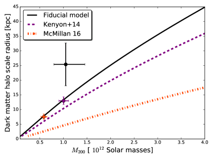
Figure 5: Dark Halo mass ($M_{\rm 200}$) versus dark matter scale radius ($r_{\rm s}$) for 3 different models for the Galactic potential: the model presented in Section 4 (“Fiducial model"), the one adopted by Kenyon et al. (2014) and one which combines our disc model and a symmetric average of the bulge matter density profile, as reported by McMillan (2016). The plotted lines are combinations of mass and radius that give an escape velocity from the GC of 850 km s^-1. Over-plotted in matching colours for each Galactic potential model are the best fitting parameters for the Galactic circular velocity (see Appendix A). Note that a mixed model with the McMillan (2016)’s bulge and the Kenyon et al.’s parameters for the disc gives intermediate results.

The mapping $V_{\rm G}\rightarrow(M_{\rm h}-r_{\rm s})$ depends on the assumed baryonic matter density distribution, upon which there is no full general agreement (see Bland-Hawthorn & Gerhard, 2016, for a recent observational review on the Galactic content and structure). In particular, both the total baryonic mass and its concentration can have an impact. The most recent works point towards a stellar mass in the bulge around $1-2\times 10^{10}M_{\odot}$ (e.g. Portail et al., 2015), but one should be aware of uncertainties given by the fact that different observational studies of the bulge constrain the mass in different regions and the size of the bulge is not universally defined. Moreover, the bulge’s mass is distributed in a complex box/peanut structure, coexisting with an addition spherical component (see Gonzalez & Gadotti, 2016, for an observational review on the bulge). The corresponding 3-dimensional density profile down to the sphere of influence of Sgr A*, is therefore uncertain. Likewise for the disc component, there are ongoing efforts to try and construct a fully consistent picture, that is currently missing (see Rix & Bovy, 2013, for a recent review on the stellar disc). Recent estimates place the total disc mass around $5\times 10^{10}M_{\odot}$, a factor of two lighter than the disc mass we adopt in Fig.4.

Given these uncertainties, we here explore the impact of adopting different baryonic components than the ones we assumed in Section 4, where a justification for that choices is stated. In particular, we explore lighter components, differently distributed. To do this, we compare in Figure 5 the loci of $V_{\rm G}=850$ km s^-1in the plane $(M_{\rm 200}-r_{\rm s})$, given by other two Galactic potential models that together with ours should frame a plausible uncertainty range. We chose to plot here $M_{\rm 200}$ instead of $M_{\rm h}$ as it is commonly used to indicate the Milky Way dark matter mass and it can facilitate comparisons with results from other probes.

The potential adopted by Kenyon et al. (2014) and widely used in the HVS community is shown with a dashed line: the bulge and disc components are described by our eqs. 9 and 10 but with different parameters ($M_{\rm b}=3.76\times 10^{9}M_{\odot}$, $r_{\rm b}=0.1$ kpc, $M_{\rm d}=6\times 10^{10}M_{\odot}$, $a=2.75$ kpc, $b=0.3$ kpc). Comparing the solid and dashed lines one concludes that, for a given $r_{\rm s}$, the Kenyon et al.’s model gives $\sim 30\%$ more massive haloes. We then calculate the $V_{\rm G}=850$ km s^-1iso-courve for a bulge potential advocated by McMillan (2016) plus our fiducial model for the disc (dash-dotted line). The McMillan’s bulge model adopts a total mass of $\simeq 8.9\times 10^{9}M_{\odot}$ and it is not spherically symmetric. We therefore radially average the axisymmetric density profile before computing the corresponding potential. Note that the McMillan’s bulge model is more massive than the Kenyon et al.’s one but equally concentrated, resulting in a very different density profile. Consequently, this model gives significantly more massive haloes (by a factor $\lower 2.15277pt\hbox{$\;\buildrel>\over{\sim}\;$}2$) than we obtain with either Kenyon et al.’s or our fiducial model.

We conclude that the impact of these uncertainties on the determination of the halo mass with HVS data is large and cannot be ignored. In order to put robust constraints on the dark matter halo of our Galaxy through our method a multi-parameter fit of data is therefore required where both the disc and bulge parameters need to be left free to vary. We defer this more sophisticated analyses, however, when more and better HVS data will be available.

On the positive side, the main features of the two regions in the $M_{\rm h}-r_{\rm s}$ parameter space defined by our $V_{\rm G}=850$ km s^-1remain the same, regardless of the specific baryonic potentials: the best fitting models for the circular velocity data always lie within the $V_{\rm G}<850$ km s^-1region (see crosses in Figure 5 and Appendix A), as do the EAGLE’s predictions for $\Lambda$CDM compatible haloes.

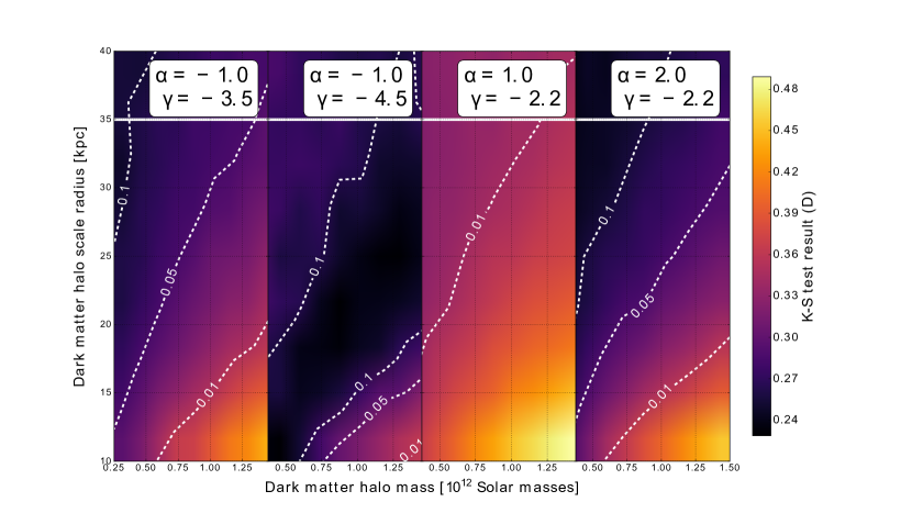
Figure 6: Contour plots for K-S test results in the parameter space $M_{\rm h}-r_{\rm s}$, for fixed $\alpha,\gamma$ pairs (see panels’ label and star marks in Figure 4). Velocity distributions are computed radially decelerating each star in a given potential (see Section 4). The white dashed lines are iso-contour lines for a given significance level $\bar{\alpha}$. Regions at the left of of each line have a value of $\bar{\alpha}$ larger than that stated in the corresponding label.

5 Discussion and conclusions

The analysis presented in the paper yields the following main results:

• For a $>5\%$ ($>1\%$) significance level fit, HVS velocity data alone require a Galactic potential with an escape velocity from the GC to 50 kpc $\lower 2.15277pt\hbox{$\;\buildrel<\over{\sim}\;$}850$ km s^-1($\lower 2.15277pt\hbox{$\;\buildrel<\over{\sim}\;$}930$ km s^-1), when assuming that binary stars within the innermost few parsecs of our Galaxy are not dissimilar from binaries in other, more observationally accessible star forming regions. For $V_{\rm G}\sim 630$ km s^-1, the binary statistics for late B-type stars observed in the Solar neighbourhood also provide a fit at the same significance level.

• When specialising to a NFW dark matter halo, we find that the region $V_{\rm G}\lower 2.15277pt\hbox{$\;\buildrel<\over{\sim}\;$}850$ km s^-1contains models that are compatible with both HVS and circular velocity data. These models also correspond to $\Lambda$CDM-compatible Milky Way haloes. In principle, we cannot exclude the parameter space $V_{\rm G}\lower 2.15277pt\hbox{$\;\buildrel>\over{\sim}\;$}850$ km s^-1. However, it would require us to face both an increasingly different statistical description of the binary population in the GC with respect to current observations and dark matter haloes that are inconsistent with predictions in the $\Lambda$CDM model at one-sigma level or more (see lower panel of Figure 4).

• The result stated in point 2 is independent of the assumed baryonic components of the Galactic potential, across a wide range for plausible masses and scale radii.

• However, the specific mapping of $V_{\rm G}$ values onto the $M_{\rm h}-r_{\rm s}$ parameter space is highly dependent on the assumed bulge and disc models (see Section 4.3). Both the baryonic total mass and its distribution affect the results. In general, works that try to infer the dark matter halo mass from HVS data should fold in the uncertainties linked to our imperfect knowledge of the baryonic mass distribution.

These results rely on certain assumptions for the binary population in the GC whose impact we now discuss. Following the same computational procedure previously presented for our fiducial model, we have found that a different mass function for the primary stars (either a Salpeter or a top-heavy mass function) or a change in metallicity (from super-solar to solar) do not substantially alter our results. However, the choice of the minimum companion mass (i.e. $m_{\rm min}$ in eq. 3) does lead to different conclusions. In particular, the higher $m_{\rm min}$, the steeper the binary distributions should be to fit the data, even for low ($<850$ km s^-1) $V_{\rm G}$. For example, for $m_{\rm min}=0.3M_{\odot}$ (instead of 0.1 $M_{\odot}$) and $V_{\rm G}=760$ km s^-1the stripe of minima for the K-S test runs along the $\gamma\approx-6.5$ and $\alpha\approx 4.5$ directions, very far from the observed values. Currently, there is no observational or theoretical reason why we should adopt a higher minimum mass than the one usually assumed (“the brown dwarf” limit), but this exercise shows that better quality and quantity HVS data has the potential to statistically constrain the minimum mass for a secondary, which may shed light on star and/or binary forming mechanisms at work in the GC.

A second set of uncertainties that may affect our conclusions pertain to the observed binary parameter distributions in the 30 Doradus region, that we use as guidance. The 30 Doradus B-type sample of Dunstall et al. (2015) is based on 6 epochs of spectra, that do not allow for a full orbital solution for each system. These authors’ results are mainly based on the distribution of the maximum variation in radial velocities per system, from where they statistically derive constraints for the full sample. Another point worth stressing is that the 30 Doradus B-type sample is of early type stars (mass roughly around $10M_{\odot}$) and distributions for late B-type star binaries in star forming regions may be different. However, these latter are not currently available, and therefore the Dustall et al. sample remains the most relevant to guide our analysis in those regions. Our statement is therefore that the statistical distributions derived from this sample (including the statistical errors on the power-law indexes) can reproduce HVS data at a several percentage confidence level. Far more reliable is the statistical description of observed late B-type binaries in the Solar neighbourhood, that can be easily reconciled with HVS data only for quite low $V_{\rm G}$ potentials.

A possibility that we have not so far discussed is that dynamical processes that inject binaries within Sgr A*’s tidal sphere modify the natal mass ratio and separation distributions. Unfortunately, as far as we know, dedicated studies are missing and we will then only discuss the consequence of the classical loss-cone theory” dealing with two-body encounters (e.g. Frank & Rees, 1976; Lightman & Shapiro, 1977) as derived in Rossi et al. (2014, section 3). Their considerations show that even allowing for extreme regimes, one would expect no modification in the mass ratio distribution and a modification in the separation distribution by no more than a factor of “a” (i.e. a natal Öpik’s law would evolve into $f_{\rm a}\sim$ const.). This would increase the $V_{\rm G}$ range ($V_{\rm G}\lower 2.15277pt\hbox{$\;\buildrel<\over{\sim}\;$}750$ km s^-1) compatible with Solar neighbourhood observations (see Fig. 2). Beside that, all our results remain unchanged.

We would also like to remark here that, although observed binary parameters give acceptable fits for $V_{\rm G}<930$ km s^-1, the K-S test results currently prefer even steeper mass ratio and binary separation distributions ($\gamma\sim-4.5$ instead of $\gamma\sim-3.5$ and/or $\alpha\sim 2$ instead of -1, see Fig. 6). This larger $|\gamma|$ value gives a steeper high velocity tail, which better match the lack of observed $>700$ km s^-1HVSs. From the above considerations, modification of the natal distribution by standard two-body scattering into the binary loss cone may not be held responsible. Assuming that the halo actually has $V_{\rm G}<930$ km s^-1, one possible inference is indeed that $\gamma\sim-4.5$ is a better description of the B-type binary natal distribution in the GC, close but not identical to that in the Tarantula Nebula.

It is of course possible that some other dynamical interactions (e.g. binary softening/hardening, collisions) or disruption of binaries in triples could be indeed responsible for a change in $\gamma$ and a larger one in $\alpha$. However, for massive binaries dynamical evolution of their properties may be neglected in the GC, because it would happen on timescales longer than their lifetime (Pfuhl et al., 2014). On the contrary, it may be relevant for low mass binaries, but only within the inner 0.1 pc (Hopman, 2009). Nevertheless, these possibilities would be very intriguing to explore in depth, if more and better data on HVSs together with a more solid knowledge of binary properties in different regions will still indicate the need for such processes.

Finally, given the paucity of data, we did not use any spatial distribution information but we rather fitted the velocity distribution integrated over the observed radial range. This precluded the possibility to meaningfully investigate anisotropic dark matter distributions and we preferred to confine ourselves to spherically symmetric potentials.

All the above uncertainties and possibilities can and should be tested and explored when a HVS data sample that extends below and above the velocity peak is available. Such a data set would allow us to break the degeneracy between halo and binary parameters, as the rise to the peak and the peak itself are mostly sensitive to the halo properties, whereas the high velocity tail is primarily shaped by the binary distributions. This will be achieved in the coming few years thanks to the ESA mission Gaia, whose catalogue should contain at least a few hundred HVSs with precise astrometric measurements. Moreover Gaia will greatly improve our knowledge of binary statistics in the Galaxy (but not directly in the GC, where infrared observations are required) and in the LMC allowing us to draw more robust inferences.

In conclusion, this paper shows for the first time the potential of HVS data combined with our modelling method to extract joint information on the GC and (dark) matter distribution. It is clear, however, that the full realisation of this potential requires a larger and less biased set of data. The ESA Gaia mission is likely to provide such a sample within the coming five years.

Appendix A Markov Chain Monte Carlo to fit the observed circular velocity

To assess which ranges of the halo mass and scale radius are compatible with current constraints of the Milky Way halo, we employ circular velocity measurements presented in Huang et al. (2016) where the rotation curve of the Milky Way out to $\sim$ 100 kpc has been constructed using $\sim$ 16,000 primary red clump giants in the outer disc selected from the LAMOST Spectroscopic Survey of the Galactic Anti-centre (LSS-GAC) and the SDSS-III/APOGEE survey, combined with $\sim$ 5700 halo K giants selected from the SDSS/SEGUE survey. These measurements are reported in Figure 7 left panel as green points with error bars.

We remind the reader that our model for the matter density (and thus the circular velocity) of the Milky Way consists of three components: a bulge, a disc, and an extended (dark matter) halo. While bulge and disc dominate the circular velocity at relatively small scales (below about 30 kpc), larger scales are dominated by the dark matter halo. Each of these components for all models we consider is described in detail in the main body of the paper (see Sections 4 and 4.3). To fit the data described above we fix the parameters that refers to the bulge and the disc, whereas we consider as free parameters those related to the dark matter halo. We remind that dark matter halo is assumed to have a NFW matter density profile, completely characterised by two parameters: the total halo mass, $M_{\rm h}$, and the scale radius, $r_{\rm s}$.

The two-dimensional parameter space $(M_{\rm h},r_{\rm s})$ is sampled with an affine invariant ensemble Markov Chain Monte Carlo (MCMC) sampler (Goodman & Weare, 2010). Specifically, we use the publicly available code Emcee (Foreman-Mackey et al., 2013). We run Emcee with three separate chains with 200 walkers and 4 500 steps per walker. Using the resulting 2 700 000 model evaluations, we estimate the parameter uncertainties. We assess the convergence of the chains by computing the auto-correlation time (see e.g. Akeret et al., 2013) and finding that our chains are about a factor of 20 times longer than it is needed to reach 1% precision on the mean of each fit parameter.

The left panel of Figure 7 shows the circular velocity as a function of distance from the GC. Green points with error bars are taken from table 3 of Huang et al. (2016), whereas orange and yellow shaded regions correspond to the 68th and 95th credibility intervals obtained from the MCMC procedure described above for our fiducial model (Section 4). Different line styles and colours refer to the different contributions as detailed in the legend. The MCMC leads to a best-fit $\chi^{2}$ of $39.07$ with $N_{\rm data}=43$ data points and $N_{\rm par}=2$ model parameters, thus resulting in a satisfactory reduced $\chi^{2}_{\rm red}=\chi^{2}/(N_{\rm data}-N_{\rm par})=0.95$. Comparable level of agreement between models and data is obtained when adopting i) a model that combines our fiducial disc parameters with a lighter bulge from McMillan (2016) ($\chi^{2}_{\rm red}=1.34$) or ii) Kenyon et al. (2014)’s much lighter disc and bulge models ($\chi^{2}_{\rm red}=0.88$).

The right panels of Figure 7 show the posterior distribution of the halo parameters for the three baryonic models mentioned above. As expected, the two halo parameters are strongly degenerate but the sampling strategy has nevertheless finely sampled the region of high likelihood. For our fiducial baryonic model, we find that ${\rm log}[M_{\rm h}/M_{\odot}]=11.89\pm 0.18$, and $r_{\rm s}=25.4\pm 7.3$ kpc, where we quote the median and errors are derived from the 16th and 84th percentiles. For i) instead the best fitting parameters are ${\rm log}[M_{\rm h}/M_{\odot}]=11.42\pm 0.06$, and $r_{\rm s}=7.5^{+1.0}_{-0.9}$ kpc, while ii) gives intermediate results: ${\rm log}[M_{\rm h}/M_{\odot}]=11.72\pm 0.06$, and $r_{\rm s}=12.99^{+1.4}_{-1.3}$ kpc.

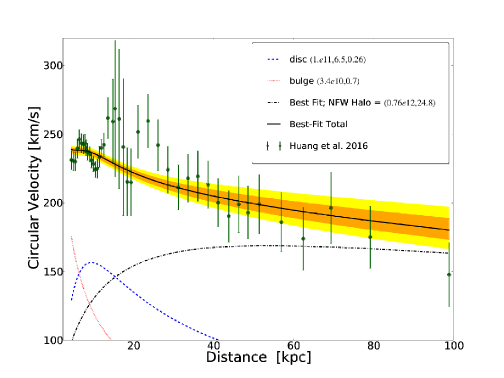
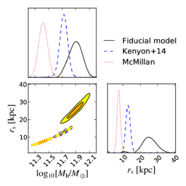
Figure 7: Left panel: Galactic circular velocity. Data points with error bars are taken from Huang et al. (2016). The orange and yellow regions correspond to the 68th and 95th credibility interval obtained with the MCMC described in the text for our fiducial Galactic Potential model. Red dotted and blue dashed lines represent the contribution from the bulge and the disc, respectively, whereas the dash-dotted black line indicates the contribution from the best-fitting NFW halo. The solid black line corresponds to the total circular velocity for the best-fitting model ($\chi^{2}_{\rm red}=0.95$). Right panel: Posterior distributions of the two halo parameters, ${\rm log_{10}[M_{h}/M_{\odot}]}$ and $r_{\rm s}$, as obtained from the MCMC used to fit the Galaxy circular velocity measurements with the three models discussed in the text (see also legend). The diagonal panels show the the posterior distributions for each parameter. The lower left panel shows the two-dimensional marginalised posterior distributions. As expected, the two parameters are strongly degenerate. Orange (yellow) region indicates the extent of the 68% (95%) credibility interval.

References

- Aarseth (1974) Aarseth S. J., 1974, A&A, 35, 237
- Akeret et al. (2013) Akeret J., Seehars S., Amara A., Refregier A., Csillaghy A., 2013, Astronomy and Computing, 2, 27
- Alexander (2005) Alexander T., 2005, Phys. Rep., 419, 65
- Bartko et al. (2010) Bartko H., et al., 2010, ApJ, 708, 834
- Blaauw (1961) Blaauw A., 1961, Bull. Astron. Inst. Netherlands, 15, 265
- Bland-Hawthorn & Gerhard (2016) Bland-Hawthorn J., Gerhard O., 2016, preprint, (arXiv:1602.07702)
- Böker (2010) Böker T., 2010, in de Grijs R., Lépine J. R. D., eds, IAU Symposium Vol. 266, Star Clusters: Basic Galactic Building Blocks Throughout Time and Space. pp 58–63 (arXiv:0910.4863), doi:10.1017/S1743921309990871
- Boylan-Kolchin et al. (2011) Boylan-Kolchin M., Bullock J. S., Kaplinghat M., 2011, MNRAS, 415, L40
- Bromley et al. (2009) Bromley B. C., Kenyon S. J., Brown W. R., Geller M. J., 2009, ApJ, 706, 925
- Brown (2015) Brown W. R., 2015, ARA&A, 53, 15
- Brown et al. (2014) Brown W. R., Geller M. J., Kenyon S. J., 2014, ApJ, 787, 89
- Bullock et al. (2010) Bullock J. S., Stewart K. R., Kaplinghat M., Tollerud E. J., Wolf J., 2010, ApJ, 717, 1043
- Carollo et al. (1997) Carollo C. M., Stiavelli M., de Zeeuw P. T., Mack J., 1997, AJ, 114, 2366
- Carson et al. (2015) Carson D. J., Barth A. J., Seth A. C., den Brok M., Cappellari M., Greene J. E., Ho L. C., Neumayer N., 2015, AJ, 149, 170
- Do et al. (2015) Do T., Kerzendorf W., Winsor N., Støstad M., Morris M. R., Lu J. R., Ghez A. M., 2015, ApJ, 809, 143
- Duchêne & Kraus (2013) Duchêne G., Kraus A., 2013, ARA&A, 51, 269
- Dunstall et al. (2015) Dunstall P. R., et al., 2015, A&A, 580, A93
- Eldridge et al. (2011) Eldridge J. J., Langer N., Tout C. A., 2011, MNRAS, 414, 3501
- Foreman-Mackey et al. (2013) Foreman-Mackey D., Hogg D. W., Lang D., Goodman J., 2013, PASP, 125, 306
- Fragione & Loeb (2016) Fragione G., Loeb A., 2016, preprint, (arXiv:1608.01517)
- Frank & Rees (1976) Frank J., Rees M. J., 1976, MNRAS, 176, 633
- Fritz et al. (2016) Fritz T. K., et al., 2016, ApJ, 821, 44
- Genzel et al. (2010) Genzel R., Eisenhauer F., Gillessen S., 2010, Reviews of Modern Physics, 82, 3121
- Georgiev & Böker (2014) Georgiev I. Y., Böker T., 2014, MNRAS, 441, 3570
- Ghez et al. (2008) Ghez A. M., et al., 2008, ApJ, 689, 1044
- Gibbons et al. (2014) Gibbons S. L. J., Belokurov V., Evans N. W., 2014, MNRAS, 445, 3788
- Gillessen et al. (2009) Gillessen S., Eisenhauer F., Trippe S., Alexander T., Genzel R., Martins F., Ott T., 2009, ApJ, 692, 1075
- Gnedin et al. (2005) Gnedin O. Y., Gould A., Miralda-Escudé J., Zentner A. R., 2005, ApJ, 634, 344
- Gnedin et al. (2010) Gnedin O. Y., Brown W. R., Geller M. J., Kenyon S. J., 2010, ApJ, 720, L108
- Gonzalez & Gadotti (2016) Gonzalez O. A., Gadotti D., 2016, Galactic Bulges, 418, 199
- Goodman & Weare (2010) Goodman J., Weare J., 2010, Comm. App. Math. Comp. Sci., 5, 65
- Guedes et al. (2011) Guedes J., Callegari S., Madau P., Mayer L., 2011, ApJ, 742, 76
- Hawkins et al. (2015) Hawkins K., et al., 2015, MNRAS, 447, 2046
- Hernquist (1990) Hernquist L., 1990, ApJ, 356, 359
- Hills (1988) Hills J. G., 1988, Nature, 331, 687
- Hopman (2009) Hopman C., 2009, ApJ, 700, 1933
- Huang et al. (2016) Huang Y., et al., 2016, preprint, (arXiv:1604.01216)
- Hurley et al. (2000) Hurley J. R., Pols O. R., Tout C. A., 2000, MNRAS, 315, 543
- Johnston et al. (1995) Johnston K. V., Spergel D. N., Hernquist L., 1995, ApJ, 451, 598
- Kafle et al. (2014) Kafle P. R., Sharma S., Lewis G. F., Bland-Hawthorn J., 2014, ApJ, 794, 59
- Kenyon et al. (2008) Kenyon S. J., Bromley B. C., Geller M. J., Brown W. R., 2008, ApJ, 680, 312
- Kenyon et al. (2014) Kenyon S. J., Bromley B. C., Brown W. R., Geller M. J., 2014, ApJ, 793, 122
- Klypin et al. (1999) Klypin A., Kravtsov A. V., Valenzuela O., Prada F., 1999, ApJ, 522, 82
- Kobayashi et al. (2012) Kobayashi S., Hainick Y., Sari R., Rossi E. M., 2012, ApJ, 748, 105
- Kobulnicky et al. (2014) Kobulnicky H. A., et al., 2014, ApJS, 213, 34
- Kouwenhoven et al. (2007) Kouwenhoven M. B. N., Brown A. G. A., Portegies Zwart S. F., Kaper L., 2007, A&A, 474, 77
- Kroupa (2002) Kroupa P., 2002, Science, 295, 82
- Laevens et al. (2015) Laevens B. P. M., et al., 2015, ApJ, 813, 44
- Law & Majewski (2010) Law D. R., Majewski S. R., 2010, ApJ, 714, 229
- Lightman & Shapiro (1977) Lightman A. P., Shapiro S. L., 1977, ApJ, 211, 244
- Loebman et al. (2014) Loebman S. R., et al., 2014, ApJ, 794, 151
- Lu et al. (2013) Lu J. R., Do T., Ghez A. M., Morris M. R., Yelda S., Matthews K., 2013, ApJ, 764, 155
- Madigan et al. (2014) Madigan A.-M., Pfuhl O., Levin Y., Gillessen S., Genzel R., Perets H. B., 2014, ApJ, 784, 23
- McMillan (2016) McMillan B. F., 2016, preprint, (arXiv:1608.05580)
- Meyer et al. (2012) Meyer L., et al., 2012, Science, 338, 84
- Miyamoto & Nagai (1975) Miyamoto M., Nagai R., 1975, PASJ, 27, 533
- Moore et al. (1999) Moore B., Ghigna S., Governato F., Lake G., Quinn T., Stadel J., Tozzi P., 1999, ApJ, 524, L19
- Muno et al. (2005) Muno M. P., Pfahl E., Baganoff F. K., Brandt W. N., Ghez A., Lu J., Morris M. R., 2005, ApJ, 622, L113
- Navarro et al. (1996) Navarro J. F., Frenk C. S., White S. D. M., 1996, ApJ, 462, 563
- Ott et al. (1999) Ott T., Eckart A., Genzel R., 1999, ApJ, 523, 248
- Paumard et al. (2006) Paumard T., et al., 2006, ApJ, 643, 1011
- Perets & Šubr (2012) Perets H. B., Šubr L., 2012, ApJ, 751, 133
- Perets et al. (2009) Perets H. B., Wu X., Zhao H. S., Famaey B., Gentile G., Alexander T., 2009, ApJ, 697, 2096
- Pfuhl et al. (2011) Pfuhl O., et al., 2011, ApJ, 741, 108
- Pfuhl et al. (2014) Pfuhl O., Alexander T., Gillessen S., Martins F., Genzel R., Eisenhauer F., Fritz T. K., Ott T., 2014, ApJ, 782, 101
- Portail et al. (2015) Portail M., Wegg C., Gerhard O., Martinez-Valpuesta I., 2015, MNRAS, 448, 713
- Price-Whelan et al. (2014) Price-Whelan A. M., Hogg D. W., Johnston K. V., Hendel D., 2014, ApJ, 794, 4
- Rimoldi et al. (2016) Rimoldi A., Portegies Zwart S., Rossi E. M., 2016, Computational Astrophysics and Cosmology, 3, 2
- Rix & Bovy (2013) Rix H.-W., Bovy J., 2013, A&A Rev., 21, 61
- Rossi et al. (2014) Rossi E. M., Kobayashi S., Sari R., 2014, ApJ, 795, 125
- Sana et al. (2012) Sana H., et al., 2012, Science, 337, 444
- Sana et al. (2013) Sana H., et al., 2013, A&A, 550, A107
- Sari et al. (2010) Sari R., Kobayashi S., Rossi E. M., 2010, ApJ, 708, 605
- Schaller et al. (2015) Schaller M., et al., 2015, MNRAS, 451, 1247
- Schaye et al. (2015) Schaye J., et al., 2015, MNRAS, 446, 521
- Schödel et al. (2014a) Schödel R., Feldmeier A., Neumayer N., Meyer L., Yelda S., 2014a, Classical and Quantum Gravity, 31, 244007
- Schödel et al. (2014b) Schödel R., Feldmeier A., Kunneriath D., Stolovy S., Neumayer N., Amaro-Seoane P., Nishiyama S., 2014b, A&A, 566, A47
- Sesana et al. (2007) Sesana A., Haardt F., Madau P., 2007, MNRAS, 379, L45
- Tauris (2015) Tauris T. M., 2015, MNRAS, 448, L6
- Vera-Ciro & Helmi (2013) Vera-Ciro C., Helmi A., 2013, ApJ, 773, L4
- Vera-Ciro et al. (2013) Vera-Ciro C. A., Helmi A., Starkenburg E., Breddels M. A., 2013, MNRAS, 428, 1696
- Wang et al. (2015) Wang W., Han J., Cooper A. P., Cole S., Frenk C., Lowing B., 2015, MNRAS, 453, 377
- Williams & Evans (2015) Williams A. A., Evans N. W., 2015, MNRAS, 454, 698
- Yu & Madau (2007) Yu Q., Madau P., 2007, MNRAS, 379, 1293
- Zhang et al. (2013) Zhang F., Lu Y., Yu Q., 2013, ApJ, 768, 153
- Zheng et al. (2014) Zheng Z., et al., 2014, ApJ, 785, L23