The Global Higgs as a Signal for Compositeness at the LHC

Abstract

The radial excitation of the global symmetry-breaking vacuum in composite Higgs models, called the “global Higgs”, has been recently a focus of investigation. In this paper we study the prospects for detecting this composite scalar at the 13 TeV LHC. We compute the global Higgs production rates and estimate the discovery potential of a global Higgs decaying into top quark pairs and into Higgs and electroweak gauge bosons with subsequent hadronic decays. The global Higgs may also decay into fermion resonances such as top partners, providing a new window into compositeness. We show that top partner jets can be effectively unresolved in some regions of the parameter space. Such “boosted top partner” signatures would deserve the development of dedicated substructure analyses.

1 Introduction

The existence of another spin-0, CP-even particle in viable composite Higgs models where the Higgs field is identified as a pseudo Nambu-Goldstone boson (pNGB) has recently been a topic of investigation in the literature Buttazzo:2015bka ; Feruglio:2016zvt ; us . This heavy state was defined in us as the “radial” excitation of the coset space parameterized by the NGBs of such models, and is referred to as the global Higgs. It is therefore intimately connected to the breaking of an (approximate) global symmetry in a new strongly-coupled sector, and identifying it would give information about this breaking, equivalent to the information we have obtained about electroweak symmetry breaking (EWSB) from the observation of the Higgs resonance at the LHC Aad:2012tfa ; Chatrchyan:2012xdj .

It has been shown in vonGersdorff:2015fta ; us that the global Higgs can consistently be amongst the lightest states of the strongly coupled theory, probably around the scale of the lowest lying fermionic resonances, and below the scale of spin-1 excitations. Moreover, it couples in a model-independent manner to the (SM) Higgs boson and to the longitudinal electroweak gauge bosons, with a sizeable strength. Interestingly, its one-loop interactions with transverse gauge bosons (in particular its couplings to gluons) can be enhanced by the large number of states running in the loops.

In this work we focus on the LHC implications of such a global Higgs particle, which could very well be the first signal of Higgs compositeness at the LHC.

Our plan is as follows. The properties of the global Higgs that are relevant for the LHC phenomenology are summarized in Sec. 2, and its main production rates are evaluated in Sec. 3. The discovery potential of the global Higgs at the $13$ TeV LHC is estimated in Sec. 4, through its decays into NGBs and top pairs. In Sec. 5, we consider the case of top partner resonant production via the global Higgs channel, and the possibility of boosted top partner signals is subsequently investigated. We conclude in Sec. 6.

2 Properties of the Global Higgs

The properties of the global Higgs were presented in Ref. us for the case of the $SO(5)/SO(4)$ coset. For concreteness, we continue focusing on this example. In this section, we summarize the features that are relevant for studying the LHC phenomenology of the global Higgs.

2.1 Tree-level couplings

The mass, vacuum expectation value (VEV) and quartic coupling of the global Higgs are denoted by $m_{\phi}$, $\hat{f}$ and $\lambda$, respectively. They are related by

$$m_{\phi}=\sqrt{2\lambda}\,{\hat{f}}~{}.$$ (1)

The NGBs of the $SO(5)\to SO(4)$ breaking, which belong to the same $SO(5)$ multiplet as the global Higgs, can mix with the longitudinal components of massive spin-1 resonances of the underlying strong dynamics. As a result, their decay constant $f$ (which controls the deviations of the pNGB Higgs from the SM limit) is expected to be smaller than $\hat{f}$ (which controls the couplings of the global Higgs). This extra degree of freedom is parameterized by

$$r_{v}=\frac{f^{2}}{\hat{f}^{2}}\,,\quad\textrm{where}\quad r_{v}\leq 1~{}.$$ (2)

Among the SM particles, the global Higgs couples mainly to the $SO(5)/SO(4)$ NGBs, i.e. to the Higgs boson and the longitudinal polarizations of the $W$ and $Z$, and to the top quark. The corresponding couplings are read from

$${\cal L} \supset 2\frac{r_{v}}{\hat{f}}\,\phi\,|D_{\mu}H|^{2}-\frac{m_{t}}{\hat{f}}\phi\,\bar{t}t~{}.$$ (3)

These depend on two independent parameters, $\hat{f}$ and $r_{v}$, and lead to the 2-body decay widths (neglecting EWSB effects):

$$\Gamma_{\phi\rightarrow hh}~{}=~{}\Gamma_{\phi\rightarrow Z_{L}Z_{L}}~{}=~{}\frac{1}{2}\,\Gamma_{\phi\rightarrow W_{L}^{+}W_{L}^{-}}~{}=~{}\frac{r_{v}^{2}}{32\pi}\frac{m_{\phi}^{3}}{\hat{f}^{2}}~{},$$ (4)

and

$$\Gamma_{\phi\rightarrow t\bar{t}}=N_{c}\frac{m_{t}^{2}}{8\pi\hat{f}^{2}}\,m_{\phi}~{}.$$ (5)

The global Higgs also couples to the heavy fermion and vector resonances of the theory. The vector resonances affect the global Higgs phenomenology mainly at loop level, to be discussed in the next subsection. Regarding the spin-$1/2$ resonances, however, one should keep in mind that the global Higgs can have a sizeable branching fraction into a fermion resonance plus a SM fermion $\phi\rightarrow\psi_{\rm SM}\bar{\psi}$, $\phi\rightarrow\psi\bar{\psi}_{\rm SM}$, or into two heavy fermion resonances $\phi\rightarrow\psi\bar{\psi}$, provided such decays are kinematically allowed. The precise branching fractions are highly model-dependent, but when open such channels typically dominate the decay modes of the global Higgs.

2.2 Loop-induced couplings

The heavy resonances induce additional couplings of the global Higgs to the SM gauge fields. These can be parameterized by local operators as follows:

$${\cal L}\supset-\phi\left(\frac{a_{gg}}{\hat{f}}\,(G^{a}_{\mu\nu})^{2}+\frac{a_{WW}}{\hat{f}}\,W^{+}_{\mu\nu}W^{-\mu\nu}+\frac{a_{ZZ}}{\hat{f}}\,(Z_{\mu\nu})^{2}+\frac{a_{\gamma\gamma}}{\hat{f}}\,(F_{\mu\nu})^{2}+\frac{a_{\gamma Z}}{\hat{f}}\,F_{\mu\nu}Z^{\mu\nu}\right)~{},$$ (6)

where the coefficients $a_{i}$ depend on the detailed spectrum of heavy resonances. The most important of these, from a phenomenological point of view, is the coupling to gluons which plays a crucial role in the production of the global Higgs at the LHC. The above include also couplings to two photons and to the transverse degrees of freedom of the $W$ and $Z$ vector bosons, which can play a non-negligible role in some regions of the parameter space.

The contribution to the $a_{i}$ due to vector resonances depends only on the $SO(5)/SO(4)$ coset structure. We expect these spin-1 resonances to be heavy compared to the global Higgs, which implies that the corresponding contribution depends only on $r_{v}$ us .

The fermion contribution, on the other hand, depends on the specifics of the fermionic sector. Instead of trying to perform a detailed analysis by scanning over the full set of microscopic parameters of given models, we will establish a reasonable “model-independent” estimate that captures the expected size of the $a_{i}$’s within a factor of order one, at least in the bulk of the natural parameter space of the models we envision (see later). This will also allow us to explore the potential enhancements due to the multiplicity of resonances that get part of their mass from the breaking of the global symmetry. Following Ref. us , we first note that the $a_{i}$’s can be usefully thought as containing two distinct ingredients. First, the 1-loop integral itself depends only on the physical fermion masses, $M_{i}$, and on the global Higgs mass, through the combination $\tau_{i}=m^{2}_{\phi}/(4M^{2}_{i})$. When the $M_{i}$ are of order, or larger than $m_{\phi}$, the (dimensionless) loop-function, commonly denoted by $A_{1/2}(\tau_{i})$ and given in App. A, displays a mild dependence on $M_{i}$. For instance, when $0.6\,m_{\phi}\lesssim M_{i}<\infty$, the loop function $A_{1/2}(\tau_{i})$ deviates by at most $20\%$ from its value at $M_{i}=m_{\phi}$. For the cases of interest in this work, we can parametrize the scale of heavy fermionic resonances by a single “average” mass scale that we denote by $\bar{M}_{\psi}$, and take the loop function as (approximately) universal: $A_{1/2}(\tau_{i})\approx A_{1/2}(m^{2}_{\phi}/(4\bar{M}^{2}_{\psi}))$. The second, more important ingredient, is the actual coupling of any given fermionic resonance to the global Higgs. Such a coupling depends on the underlying (proto-)Yukawa coupling and on an angle that characterizes the mixing between different $SO(4)$ representations. The mixing angle parametrizes the fraction of the fermion mass coming from the breaking of the global symmetry, and therefore describes the decoupling properties of these virtual effects. Under the assumption discussed above of a universal loop function, we can use well known sum rules to define a convenient reference fermion scale, $M_{\psi}$. For example, for the gluon fusion process, we write

$$\hat{f}\,\sum_{i}\frac{M_{i}^{\prime}}{M_{i}}=-2\frac{\hat{f}^{2}}{M_{\psi}^{2}}\left(\bar{N}^{U}_{\phi gg}\operatorname{tr}\xi_{U}^{\prime}\xi_{U}^{T}+\bar{N}^{D}_{\phi gg}\operatorname{tr}\xi^{\prime}_{D}\xi_{D}^{T}\right)~{},$$ (7)

where $M_{i}^{\prime}=dM_{i}/d\hat{f}$ and the proto-Yukawa couplings, $\xi^{(\prime)}_{U}$ and $\xi^{(\prime)}_{D}$, were defined in us . There are similar expressions for $\phi BB$ and $\phi\gamma\gamma$, where the sums are now weighted by the square of the hypercharges and charges, respectively (see Ref. us for the explicit expressions). The trace is over generations, and the $N^{U,D}_{A}$, with $A=\phi gg$, $\phi BB$ and $\phi\gamma\gamma$ characterize the multiplicity effect of a given tower of resonances associated with the up or down sectors. Analogous leptonic multiplicities, $N^{E}_{A}$, enter into the $\phi BB$ and $\phi\gamma\gamma$ processes. Since $M_{\psi}$ and $\bar{M}_{\psi}$ are typically close, we simply take $\bar{M}_{\psi}=M_{\psi}$ in the fermion loop functions, where in practice we think of $M_{\psi}$ as being defined by the gluon fusion process.

Putting the previous ingredients together, we write

$$a_{gg}=-c_{gg}\,\frac{\hat{f}^{2}}{M_{\psi}^{2}}\,A_{1/2}\!\left(\frac{m_{\phi}^{2}}{4M_{\psi}^{2}}\right)~{},\quad a_{BB}=-c_{BB}\,\frac{\hat{f}^{2}}{M_{\psi}^{2}}\,A_{1/2}\!\left(\frac{m_{\phi}^{2}}{4M_{\psi}^{2}}\right)~{},$$ (8)

$$a_{\gamma\gamma}=-c_{\gamma\gamma}\,\frac{\hat{f}^{2}}{M_{\psi}^{2}}\,A_{1/2}\!\left(\frac{m_{\phi}^{2}}{4M_{\psi}^{2}}\right)-0.0022\,(1-r_{v})\,,$$ (9)

together with the $SU(2)_{L}\times U(1)_{Y}$ relations

$$a_{WW}=\frac{2}{s^{2}_{W}}(a_{\gamma\gamma}-c^{2}_{W}a_{BB})~{},~{}a_{ZZ}=\frac{1}{2}\,c^{2}_{W}a_{WW}+s^{2}_{W}a_{BB}~{},~{}a_{\gamma Z}=s_{W}c_{W}(a_{WW}-2a_{BB})~{}.$$ (10)

In Eq. (9) we used that $(\alpha/8\pi)A_{1}\approx 0.0022$ in the asymptotic limit where $A_{1}\rightarrow-7$. The $c_{i}$ coefficients are given by

$$c_{gg} = \frac{\alpha_{s}}{8\pi}\left(\bar{N}^{U}_{\phi gg}\operatorname{tr}\xi_{U}^{\prime}\xi_{U}^{T}+\bar{N}^{D}_{\phi gg}\operatorname{tr}\xi^{\prime}_{D}\xi_{D}^{T}\right)~{},$$

$$c_{BB} = \frac{\alpha}{4\pi c^{2}_{W}}\left(N_{c}\,\bar{N}^{U}_{\phi BB}\operatorname{tr}\xi_{U}^{\prime}\xi_{U}^{T}+N_{c}\,\bar{N}^{D}_{\phi BB}\operatorname{tr}\xi^{\prime}_{D}\xi_{D}^{T}+\bar{N}^{E}_{\phi BB}\operatorname{tr}\xi_{E}^{\prime}\xi_{E}^{T}\right)~{},$$ (11)

$$c_{\gamma\gamma} = \frac{\alpha}{4\pi}\left(N_{c}\,\bar{N}^{U}_{\phi\gamma\gamma}\operatorname{tr}\xi_{U}^{\prime}\xi_{U}^{T}+N_{c}\,\bar{N}^{D}_{\phi\gamma\gamma}\operatorname{tr}\xi^{\prime}_{D}\xi_{D}^{T}+\bar{N}^{E}_{\phi\gamma\gamma}\operatorname{tr}\xi_{E}^{\prime}\xi_{E}^{T}\right)~{},$$

where $N_{c}=3$ is the number of colors, $\alpha_{s}$ is the strong coupling constant, $\alpha$ is the fine structure constant, and the multiplicities, $N^{U,D,E}_{A}$, with $A=\phi gg$, $\phi BB$ and $\phi\gamma\gamma$ encode the model-dependence (to be discussed next).

The partial decay widths into transverse gauge bosons are given by

$$\Gamma_{\phi\rightarrow gg}=\frac{2a_{gg}^{2}}{\pi}\,\frac{m_{\phi}^{3}}{\hat{f}^{2}}~{},$$ (12)

$$\Gamma_{\phi\rightarrow\gamma\gamma}=\frac{a_{\gamma\gamma}^{2}}{4\pi}\,\frac{m_{\phi}^{3}}{\hat{f}^{2}}~{},\quad\quad\Gamma_{\phi\rightarrow Z_{T}Z_{T}}=\frac{a_{ZZ}^{2}}{4\pi}\,\frac{m_{\phi}^{3}}{\hat{f}^{2}}~{},$$ (13)

$$\Gamma_{\phi\rightarrow\gamma Z_{T}}=\frac{a_{\gamma Z}^{2}}{8\pi}\,\frac{m_{\phi}^{3}}{\hat{f}^{2}}~{},\quad\quad\Gamma_{\phi\rightarrow W_{T}^{+}W_{T}^{-}}=\frac{a_{WW}^{2}}{8\pi}\,\frac{m_{\phi}^{3}}{\hat{f}^{2}}~{}.$$ (14)

2.3 Benchmark scenarios

In Ref. us , we defined a number of fermion realizations, which differ by the $SO(5)$ embeddings of the fermion partners and of the global Higgs. These benchmark scenarios are defined by

$\bullet$  MCHM5,1,10:	$(Q_{i},U_{i},D_{i})=({\bf 5}_{\frac{2}{3}},{\bf 1}_{\frac{2}{3}},{\bf 10}_{\frac{2}{3}})$ ,	$\phi\subset{\bf 5_{0}}$ ,
$\bullet$  MCHM5,14,10:	$(Q_{i},U_{i},D_{i})=({\bf 5}_{\frac{2}{3}},{\bf 14}_{\frac{2}{3}},{\bf 10}_{\frac{2}{3}})$ ,	$\phi\subset{\bf 5_{0}}$ ,
$\bullet$  MCHM14,14,10:	$(Q_{i},U_{i},D_{i})=({\bf 14}_{\frac{2}{3}},{\bf 14}_{\frac{2}{3}},{\bf 10}_{\frac{2}{3}})$ ,	$\phi\subset{\bf 14_{0}}$ ,
$\bullet$  MCHM5,1:	$(Q_{3},U_{3})=({\bf 5}_{\frac{2}{3}},{\bf 1}_{\frac{2}{3}})$ ,	$\phi\subset{\bf 5_{0}}$ ,

where we indicate the $SO(5)$ representations and $U(1)_{X}$ charges of the “partners” of the SM $SU(2)_{L}$ quark doublets and up-type quark and down-type quark singlets, as well as of the global Higgs multiplet. The precise embedding of the lepton sector affects the electroweak channels, such as $\phi\to\gamma\gamma$, $\phi\to\gamma Z_{T}$ and $\phi\to V_{T}V_{T}$, and we refer the reader to Ref. us for illustrative benchmarks. We will use the multiplicities $\bar{N}^{U,D,E}_{\phi\gamma\gamma}$ and $\bar{N}^{U,D,E}_{\phi BB}$ computed in that reference, and reproduced in Table 1. The last model defined above, MCHM_5,1, is a “non-anarchic” scenario where only the top quark resonances give a non-negligible effect. Further details can be found in us .

Benchmark	$\bar{N}^{U}_{\phi gg}$	$\bar{N}^{D}_{\phi gg}$	$\bar{N}^{U}_{\phi\gamma\gamma}$	$\bar{N}^{D}_{\phi\gamma\gamma}$	$\bar{N}^{E}_{\phi\gamma\gamma}$	$\bar{N}^{U}_{\phi BB}$	$\bar{N}^{D}_{\phi BB}$	$\bar{N}^{E}_{\phi BB}$
MCHM5,1,10	1	2	$\frac{4}{9}$	$\frac{17}{9}$	1	$\frac{4}{9}$	$\frac{25}{18}$	1
MCHM5,14,10	$\frac{14}{5}$	2	$\frac{101}{45}$	$\frac{17}{9}$	1	$\frac{157}{90}$	$\frac{25}{18}$	1
MCHM14,14,10	$\frac{27}{20}$	$\frac{5}{4}$	$\frac{57}{40}$	$\frac{85}{72}$	1	$\frac{81}{80}$	$\frac{125}{144}$	1
MCHM5,1	1	$-$	$\frac{4}{9}$	$-$	$-$	$\frac{4}{9}$	$-$	$-$

Table 1: Fermionic multiplicity factors entering the effective couplings of the global Higgs to two gluons or two EW gauge bosons. Reproduced from Ref us .

We will make the reasonable assumption that the vector-like masses are of the same order for all the resonances. We then note that when the global symmetry breaking effects are small compared to such vector-like masses, and when the mixing between the elementary and composite sectors is small (as may be expected for the quarks other than the top quark), the scale $M_{\psi}$ in Eq. (7) coincides with the “universal” vector-like mass. When either the elementary composite mixing is large (as would be the case for the top sector) or if the global symmetry breaking contributions to the fermions masses are sizeable, the scale $M_{\Psi}$ can differ by an order one factor from the vector-like parameters. Typically, however, this scale is of the same order as the physical fermion masses and, as described above, we incur in small errors if we identify $M_{\psi}$ [defined by Eq. (7)] with the average fermion mass used in the loop function.

In reference us we also estimated for each benchmark scenario the expected size of the proto-Yukawa couplings by assuming that they are all of the same order (we call it $\xi$) and requiring perturbativity up to a scale a few times above $m_{\phi}$. This results in

$$\xi \approx 0.6\hskip 14.22636pt\textrm{for the MCHM${}_{5,1,10}$}~{},\hskip 36.98866pt\xi~{}\approx~{}0.5\hskip 14.22636pt\textrm{for the MCHM${}_{5,14,10}$}~{},$$

$$\xi \approx 0.6\hskip 14.22636pt\textrm{for the MCHM${}_{14,14,10}$}~{},\hskip 28.45274pt\xi~{}\approx~{}1.6\hskip 14.22636pt\textrm{for the MCHM${}_{5,1}$}~{},$$

with a mild dependence on the cutoff scale. Using this information, and the multiplicities quoted in Table 1, we find from Eqs. (11): 

$$c_{gg}=\begin{pmatrix}0.013\\ 0.014\\ 0.011\\ 0.010\end{pmatrix}\,,\quad c_{BB}=\begin{pmatrix}0.0057\\ 0.0063\\ 0.0058\\ 0.0028\end{pmatrix}\,,\quad c_{\gamma\gamma}=\begin{pmatrix}0.0054\\ 0.0063\\ 0.0060\\ 0.0021\end{pmatrix}\,,$$ (15)

where the four lines correspond to the four benchmarks defined above. We used here $\alpha_{s}=0.1$, $\alpha=1/127$ and $s^{2}_{W}=0.231$.

The above set of benchmark models was chosen to exhibit a broad range of multiplicities of fermionic resonances. We see, however, that the above coefficients are nearly model independent. The reason is that the same multiplicity factors entering in the triangle diagram also enter in the dominant contribution to the $\beta$-functions of the proto-Yukawa couplings. The enhancement due to the number of states is then largely compensated by the requirement to take a smaller proto-Yukawa coupling (at the scale of $m_{\phi}$), or else a Landau pole will develop too close to the scales of interest. Since the most important process for the global Higgs phenomenology is the gluon fusion process, we will simply take, based on the above findings, $c_{gg}\approx 0.01$ in our phenomenological study. We will, however, include a $K$-factor of $K\approx 2$ Djouadi:2005gi .

2.4 Parameter space

We set the decay constant of the NGBs, $f$, to its approximate experimental lower bound Panico:2015jxa

$$f=800~{}{\rm GeV}~{}.$$ (16)

This ensures that the (SM) Higgs sector is roughly consistent with the present Higgs constraints, while minimizing the fine-tuning of the electroweak scale. As discussed above, in the bulk of the parameter space of the scenarios considered, the global Higgs properties depend, to a good approximation, on three real-valued parameters that can be chosen as $m_{\phi}$, $\lambda$ and the “scale of spin-$1/2$ resonances”, $M_{\psi}$. The other parameters defined above are obtained via $\hat{f}=m_{\phi}/\sqrt{2\lambda}$ and $r_{v}=f^{2}/{\hat{f}}^{2}$. One should also remember that

$$\hat{f}\geq f~{}.$$ (17)

Also, the same type of argument based on RG running that was used to constrain the proto-Yukawa couplings $\xi$ can be used to determine a range for the global Higgs quartic coupling. Although the range is model-dependent, as described in us , it will be sufficient to take $\lambda\in[0.2,3]$, which falls in the correct ballpark for the benchmark models defined above.

It is useful to note here that the loop-level couplings scale like $\hat{f}^{2}/M_{\psi}^{2}\sim(m_{\phi}^{2}/M_{\psi}^{2})\times\lambda^{-1}$. Therefore, they become more important for smaller $\lambda$. On the other hand, the tree-level couplings scale like $1/\hat{f}^{2n}\sim\lambda^{n}/m_{\phi}^{2n}$ for a positive power, $n$. Therefore, they become more important for larger $\lambda$. This competition will be reflected in our later results.

Figure 1: Regions in the $m_{\phi}-\lambda$ plane where the global Higgs decays dominantly into NGBs or $t\bar{t}$ pairs, assuming that all fermion resonances are heavier than the global Higgs. We take $f=800$ GeV. The shaded region below the $\hat{f}=3f$ line requires a large hierarchy between $\hat{f}$ and $f$, and may not be realized in typical strongly coupled scenarios. We also show a current bound adapted from the ATLAS heavy Higgs search of Ref. ATLAS-CONF-2013-013 , which shows that the global Higgs must be heavier than about $750$ GeV.

2.5 2-parameter case

Before we undertake a study of global Higgs production, we can immediately exhibit the relative importance of the decay channels of the global Higgs when the fermion resonances, $\psi$, are too heavy for any of the decays $\phi\rightarrow\psi_{\rm SM}\bar{\psi}$, $\phi\rightarrow\psi\bar{\psi}_{\rm SM}$, or $\phi\rightarrow\psi\bar{\psi}$ to be open. The decays are then dominated by the $WW$, $ZZ$, $hh$ and $t\bar{t}$ channels, as dictated by Eqs. (4) and (5), since the loop-induced processes are always subdominant. As usual, in the region where the equivalence theorem applies, one has that the decays into $WW$, $ZZ$ and $hh$ are in the proportion $2:1:1$. However, since these partial widths scale like $r_{v}^{2}m_{\phi}^{3}/\hat{f}^{2}\sim\lambda^{3}f^{4}/m_{\phi}^{3}$, while the partial decay width into top pairs scales like $m_{t}^{2}m_{\phi}^{2}/\hat{f}^{2}\sim m_{t}^{2}\lambda/m_{\phi}$, we see that there is a non-trivial dependence in the $m_{\phi}-\lambda$ plane. The branching fractions into NGB’s and $t\bar{t}$ become equal when $\lambda=(\sqrt{3}/2)m_{t}m_{\phi}/f^{2}$. In Fig. 1 we show in green the region dominated by the decays into NGBs, and in red the region dominated by decays into top pairs. We mark in gray the forbidden region where $\hat{f}<f$, and also show for reference the line where $\hat{f}=3f$ to indicate that typically one would not expect a large hierarchy between $\hat{f}$ and $f$. In any case, we see that the natural region of parameter space allows for a large range of possibilities, although if the global Higgs is on the heavy side of the shown range perhaps one should expect its decays to be dominated by the NGB channels.

We also note that in the case where the decays into fermion resonances are closed, the decay width of the global Higgs is at most $\Gamma_{\rm tot}/m_{\phi}=O(0.1)$, so that the narrow width approximation roughly applies. If decay channels involving the fermion resonances were open – either mixed SM - resonance final states or a pair of resonances – these channels can dominate and the global Higgs becomes a broad resonance that can reach $\Gamma_{\rm tot}/m_{\phi}=O(1)$ us .

3 The Global Higgs at the LHC

The production modes of the global Higgs at the LHC have some similarities to those of the Standard Model Higgs boson. We focus on inclusive resonant production

$$pp\rightarrow\phi^{*}+X\rightarrow Y+X~{},$$ (18)

where $\phi^{*}$ means that the intermediate $\phi$ can be off-shell, $Y$ represents the global Higgs decay products and $X$ denotes other final states resulting of the proton collision. Similarly to the SM Higgs, the global Higgs can be produced through gluon fusion (ggF), vector boson fusion (VBF), associated production with a vector boson, and in association with a $t\bar{t}$ pair. In principle, it could also be produced in association with other fermion resonances, but such production modes would be highly suppressed due to the large masses involved. The most important production modes are ggF and VBF, so we focus on these two cases.

Although, as already mentioned, the global Higgs can be either a narrow or broad resonance, typically with $\Gamma_{\rm tot}/m_{\phi}$ ranging from $O(10^{-3})$ to $O(1)$, we restrict here to the narrow resonance case. This will be sufficient for a detailed study of scenarios where decays involving heavy resonances are closed. Our later remarks for cases where some such channels are open will be treated separately.

In a large region of parameter space, the global Higgs production is dominated by the gluon fusion process

$$gg\rightarrow\phi~{},$$ (19)

controlled by the loop-induced effects discussed in the previous section. As explained there, this introduces one additional parameter beyond $m_{\phi}$ and $\lambda$: the scale of fermionic resonances, $M_{\psi}$. Recall that the loop-induced couplings scale like $1/\lambda$ and therefore become larger for smaller $\lambda$.

The VBF production mode

$$qq^{\prime}\rightarrow\phi+qq^{\prime}~{},$$ (20)

can proceed through tree-level couplings, which scale with $\lambda$ like $\lambda^{3}$, so that they can become important for larger $\lambda$. Note also that, as a function of $m_{\phi}$, these couplings scale like $1/m^{3}_{\phi}$, for fixed $f$ and $\lambda$, and therefore decrease quickly for a heavier global Higgs. There are also loop-level couplings (to transverse vector bosons and photon pairs) that scale like $1/\lambda$ and can become important at smaller $\lambda$.

In order to asses the interplay of these production modes, we simulate the production rates using MadGraph5 MG , based on a FeynRules FR implementation of the global Higgs Lagrangian. The parton density function set used is NN23LO1 Ball:2013hta , with a factorization scale set to $\mu_{F}=m_{\phi}$. The ggF and VBF production rates are shown in Fig. 2 in the cases $M_{\psi}=m_{\phi}$ (red curves) and $M_{\psi}=2m_{\phi}$ (purple curves). All the bounds on the parameters described in Sec. 2 are taken into account. In particular, for a given $\lambda$, the global Higgs mass is bounded from below by $m_{\phi}>\sqrt{2\lambda}f$ , where $f=800$ GeV.

In the VBF case, the dominance of the loop induced operators $\phi(V^{\mu\nu})^{2}$ over $\phi|D^{\mu}H|^{2}$ can be recognized by the cross-section dependence with respect to the heavy fermion mass $M_{\psi}$. This feature tends to happens for small $\lambda$, as expected. Also, the VBF rate is much smaller than the ggF rate at small $\lambda$, while it dominates at large $\lambda$. The crossover occurs around $\lambda\sim 1$.

We see that the total production rate is high enough to motivate a more precise study of the LHC implications of the presence of a global Higgs. In the following, since the VBF process is important only for large $\lambda$, we choose to focus on a $\phi+Y$ final state, without requiring forward jet tagging.

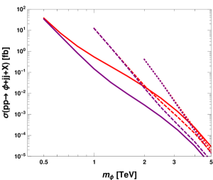
Figure 2: Global Higgs production rates via gluon fusion (left) and vector-boson fusion (right), as a function of the global Higgs mass. Red and purple lines correspond to $M_{\psi}=m_{\phi}$ and $M_{\psi}=2m_{\phi}$, respectively. Plain, dashed and dotted lines correspond to $\lambda=0.2$, $\lambda=1$, $\lambda=3$, respectively.

The LHC signals of the global Higgs can be split into two broad cases:

• Case I: All decays involving fermion resonances are closed. The phenomenology is then largely independent of the details of the heavy fermion sector, and the narrow width approximation applies. We study this case in Sec. 4.

• Case II: Some decays involving fermion resonances are open, and the phenomenology depends strongly on the realization of the fermion sector. Some generic aspects of this case will be discussed in Sec. 5.

4 Global Higgs Discovery Prospects: Decays into SM Particles

In this section we provide an estimate of the LHC sensitivity for detecting the global Higgs at a center-of-mass energy of 13 TeV and with 300 fb^-1 of integrated luminosity, assuming that all decays involving fermion resonances are kinematically forbidden. We will take $M_{\psi}=m_{\phi}$ for definiteness, and we will therefore present our results in the $m_{\phi}-\lambda$ plane. The main decay channels to be investigated, $\phi\to hh,ZZ,W^{+}W^{-},t\bar{t}$, were discussed in Fig. 1, which shows the dominant channels in different regions of parameter space. Here we explore them in more detail.

4.1 The Hadronic NGB Channel

We start by considering the case where the global Higgs decays dominantly into NGBs, i.e.

$$\phi\rightarrow W_{L}W_{L},Z_{L}Z_{L},hh\,.$$ (21)

The $W_{L}W_{L}$, $Z_{L}Z_{L}$ or $hh$ final states will decay further and therefore there is a variety of final states that can be considered. Decays into leptons could in principle provide very clean signatures. Since the overall leptonic branching fractions are rather small we focus on fully hadronic decay modes, which may be more relevant for discovery. The branching fractions of the $WW$, $ZZ$ and $hh$ states into fully hadronic final states are all roughly $50\%$. Extrapolations of 8 TeV LHC bounds in the leptonic channels can be found in Ref. Buttazzo:2015bka .

Before going into the details of the analysis it is worth pointing out that the $WW$ and $ZZ$ channels are also one of the main discovery channels for spin-1 resonances in composite Higgs models. Should a resonance be detected in this channel, a more detailed analysis will be required to discriminate between these cases. One such possibility is to look for specific channels that are forbidden in the spin-1 case, such as the decay into two photons (which is not allowed because of the Landau-Yang theorem), or the decay into two Higgses (which is forbidden because of Bose symmetry). Secondly, neutral spin-1 states typically come together with charged ones that are only split in mass by electroweak breaking effects, while possible partners of the Global Higgs are split by the larger $SO(5)\to SO(4)$ breaking. Finally, the final-state angular distribution can be used to discriminate the spin of the decaying particle, which would of course be a rather challenging task. We will not discuss further these possibilities in this paper, but rather focus on the LHC phenomenology of the Global Higgs alone.

Since we are interested in the case where $m_{\phi}\gg m_{W},m_{Z},m_{h}$, the produced $W$, $Z$ and $h$ are typically highly boosted and their hadronic decay products are collimated in the detector frame, forming a single, large-radius jet. These are usually called fat jets in the literature. In order to maximize the signal rate, we suggest searching for these fat jets. In the following, a fat jet is denoted by $J$ while a standard jet is denoted by $j$. The process we are interested in is thus

$$pp\rightarrow\phi^{*}\rightarrow JJ~{}.$$ (22)

The fully hadronic analysis is very challenging. We describe below a simple way to estimate the LHC reach for discovery of the global Higgs in these modes. We will rely on the recent progress accomplished with jet substructure techniques Butterworth:2008iy which show a promising potential for QCD background rejection. Such techniques have been applied to the search of pairs of boosted weak bosons by the ATLAS collaboration in the fully hadronic channel ATLAS_note , and we will use some of their results, especially the efficiency of tagging boosted gauge bosons in the jet samples.

The signal is computed using our implementation of the effective operators discussed in Sec. 2. For a resonance decaying into either $ZZ$ or $WW$ states, the signal efficiency for the corresponding diboson-tagged hadronic final states has been estimated in Ref. ATLAS_note at $9-10\%$ (with a 20% uncertainty). This efficiency includes the tagging as either a $[ZZ]$ selection or as a $[WW]$ selection, as defined by ATLAS ATLAS_note , while we only require tagging as a diboson event, which we denote as $[VV]$. Using the jet-tagging conditional probabilities computed in Ref. Fichet:2015yia (see also Allanach:2015hba ) we can substitute the $[WW]$ or $[ZZ]$ tagging for a $[VV]$ tagging by multiplying the $WW$ efficiency by $P(\,[VV]\,|WW)/P(\,[WW]\,|WW)$ and similarly for the $ZZ$ efficiency. The efficiencies obtained in this way are $\sim 11-12\%$, so that the overall efficiency that allows for both $WW$ and $ZZ$ final states, without trying to tell them apart, turns out to be similar to the efficiencies found in the ATLAS analysis. We assume that these efficiencies will not change significantly in the 13 TeV run, and we use $12\%$ for the $WW$ and $ZZ$ channels as well as for the $hh$ channel. ATLAS also estimates the average background selection efficiency of the tagger in simulated QCD dijet events satisfying the same cuts to be roughly $0.01\%$, showing the power of the jet substructure tools.

We turn now to a more detailed discussion of the dominant QCD background. In order to obtain a realistic dijet background for this search, the whole process of jet reconstruction, grooming, filtering and tagging should be accurately simulated. As an alternative to a complete simulation, we estimate the $JJ$ background at 13 TeV from the $JJ$ background obtained in the 8 TeV dijet analysis by ATLAS ATLAS_note . We describe next how to obtain both the shape and the normalization of the 13 TeV dijet background.

Let us start with the background distribution shape, expressed as a function of the invariant mass of the reconstructed dijet system $m_{JJ}$. The observed distribution was fit by ATLAS ATLAS_note to an analytic function $f(m_{JJ}/\sqrt{s})$, so that the $m_{JJ}$ distribution scales roughly as the center-of-mass energy. We have checked this scaling behavior with a parton-level simulation of dijet production. Hence, we can use the background shape of the 8 TeV analysis with a simple rescaling $f(m_{JJ})\rightarrow f(13/8\,m_{JJ})$. One should note that the ATLAS analysis of the 8 TeV data involves a $p_{T}$ cut on the leading jet, $p_{T}(j)>540$ GeV. This cut leads to $m_{JJ}>1080$ GeV since a cut $p_{T}>p_{T}^{\rm min}$ implies $m_{JJ}>2p_{T}^{\rm min}$, and also slightly deforms the $m_{JJ}$ distribution at low invariant mass. Therefore, in order to extrapolate the background from 8 to 13 TeV, we also have to rescale the $p_{T}$ cut on the leading jet by $13/8$, thus taking $p_{T}>877$ GeV. This in turn implies a cut $m_{JJ}>1754$ GeV at $\sqrt{s}=13$ TeV.

With the shape determined as above, we have to fix the overall normalization of the dijet background at 13 TeV. We need first the total number of events obtained after tagging two jets as weak bosons in the ATLAS 8 TeV analysis. The total number of events has been reported in ATLAS_note in three overlapping categories: $WW$, $ZZ$, $WZ$, with $\hat{n}_{WW}=425$, $\hat{n}_{ZZ}=333$, $\hat{n}_{WZ}=604$. The statistics of the overlapping event numbers for the $n_{WW}$, $n_{ZZ}$, $n_{WZ}$ categories has been thoroughly studied in Fichet:2015yia . Knowing the tagging probabilities, a simple likelihood analysis like the one described in Fichet:2015yia provides the underlying number of jets before tagging, ${\hat{n}}_{JJ}=107539$. This number can then be multiplied by the total mis-tagging probability of QCD jets into weak bosons $P([VV]|JJ)=P([V]|J)^{2}=6.4\times 10^{-3}$ obtained in Fichet:2015yia , giving the overall normalization of the 8 TeV dijet background for hadronically decaying dibosons: ${\hat{n}}_{JJ}(8\,{\rm TeV})=688$. This allows us to estimate $\sigma_{JJ}^{\rm ATLAS}(8\,{\rm TeV})=33.9$ fb.

We stress that this number corresponds to events with a $p_{T}(j)>540$ GeV cut. In order to proceed with the extrapolation, we rescale this number by the ratio of partonic cross-sections from 8 and 13 TeV, including the rescaled $p_{T}$ cut discussed above,

$$\sigma^{\rm parton}_{JJ}(13\,{\rm TeV})/\sigma^{\rm parton}_{JJ}(8\,{\rm TeV})~{}\approx~{}0.3~{}.$$ (23)

One notices the well-known feature that this ratio is smaller than one – see e.g. the general LHC cross-section plots Stirling_XS_plots . The total event rate at 13 TeV extrapolated from the ATLAS analysis is then given by

$$\sigma_{JJ}^{\rm ATLAS}(13\,{\rm TeV})~{}=~{}\sigma_{JJ}^{\rm ATLAS}(8\,{\rm TeV})\,\frac{\sigma_{JJ}^{\rm parton}(13\,{\rm TeV})}{\sigma_{JJ}^{\rm parton}(8\,{\rm TeV})}~{}\approx~{}10\;\mbox{fb}~{}.$$ (24)

With this information, we have fixed the inferred $m_{JJ}$ distribution at 13 TeV with a cut $m_{JJ}>1754$ GeV. We will then simply use the analytic fit to extrapolate the background to the $m_{JJ}<1754$ GeV region.

Finally, various realistic improvements on background rejection based on jet substructure techniques have been pointed out in Ref. Goncalves:2015yua . A simple improvement is to reduce the radius of the cone algorithm for the first step of jet identification. Indeed, the radius of a jet from weak bosons is typically $\Delta R\sim m_{V}/p_{T}\sim 0.4$ at $8$ TeV. Using the simulation of Goncalves:2015yua , we find that the mis-tagging rate $P(V|J)$ can be reduced by a factor $\sim 0.5$, when taking $\Delta R=0.4$ instead of $\Delta R=1.2$. We will assume that this improvement takes place, so that the dijet background is reduced by $(0.5)^{2}$. We regard our estimated background as roughly representative of what will be obtained at the 13 TeV LHC run. The 13 TeV extrapolated background can be seen in Fig. 3.

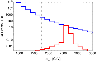
Figure 3: Projection of the dijet background at $13$ TeV extrapolated from an ATLAS $8$ TeV analysis ATLAS_note . To the left of the vertical dotted line the background is extrapolated using the model obtained in that reference. A signal for $pp\rightarrow\phi\rightarrow JJ$ assuming $f=800$ GeV, $\lambda=0.2$, $m_{\phi}=2640$ GeV is shown in red.

In order to assess discovery, we use an actual hypothesis test instead of a p-value significance test. The background-only hypothesis is denoted by $H_{0}$. The hypothesis that a signal exists is denoted by $H_{1}$ and is parameterized via $(m_{\phi},\lambda)$. The hypothesis test we employ is the discovery Bayes factor

$$B_{0}=\frac{P({\rm data}|H_{1})}{P({\rm data}|H_{0})}=\frac{\int L(m_{\phi},\lambda)\pi(m_{\phi})\pi(\lambda)\,dm_{\phi}d\lambda}{L_{\textrm{bg-only}}}~{},$$ (25)

where the likelihood function $L$ is obtained from the product of the Poisson likelihoods in each bin, and we use flat logarithmic prior density functions, $\pi$’s, for the $\lambda$ and $m_{\phi}$ parameters, with ranges $\lambda\in[0.2,3]$ and $m_{\phi}\in[0.4,4]$ TeV, respectively. The denominator $L_{\textrm{bg-only}}$ can be obtained from $L(m_{\phi},\lambda)$ by taking $m_{\phi}\to\infty$.

Following Ref. Cowan:2010js , we assume that our projected data have no statistical fluctuations (i.e. they are “Asimov” data) arising from a signal with underlying parameters $(m_{\phi}^{\prime},\lambda^{\prime})$. For each value of the parameters $(m_{\phi}^{\prime},\lambda^{\prime})$, one performs a Bayesian discovery test to evaluate whether the signal contained in these hypothetical data could be detected. The discovery Bayes factor applied to the projected data takes the form

$$B_{0}(m_{\phi}^{\prime},\lambda^{\prime})=\frac{P({\rm data}(m_{\phi}^{\prime},\lambda^{\prime})|H_{1})}{P({\rm data}(m_{\phi}^{\prime},\lambda^{\prime})|H_{0})}~{}.$$ (26)

The discovery Bayes factor for the global Higgs at the 13 TeV LHC run with a luminosity of 300 fb^-1 is shown in Fig. 4. The threshold values $3$, $12$, $150$ can be roughly translated as $2$, $3$ and $5$ $\sigma$ significance levels, respectively.

Figure 4: Projected LHC sensitivities to a global Higgs signal with 300 fb^-1 at 13 TeV. The light blue region is a bound adapted from an ATLAS heavy Higgs search ATLAS-CONF-2013-013 . The light red region is a projected 95$\%$CL limit from boosted top quark searches, as extrapolated from Ref. ATLAS-CONF-2016-014 . The red, gray, yellow regions show the discovery Bayes factor for the global Higgs in the $pp\rightarrow\phi\rightarrow JJ$ channel, and correspond respectively to weak, moderate and strong evidence for the signal hypothesis.

4.2 The Boosted $t\bar{t}$ Channel

Apart from NGBs, the other main decay channel of the global Higgs is into top quark pairs,

$$\phi\rightarrow t{\bar{t}}~{}.$$ (27)

This decay channel leads to boosted tops at the LHC. A recent search for such resonant production of boosted top quark pairs has been carried out by ATLAS using $3.2$ fb^-1 of 13 TeV data ATLAS-CONF-2016-014 . For our purpose of presenting a projected sensitivity at 300 fb^-1, we extrapolate the expected 95$\%$ CL bound on $\sigma\times BR$ given in Ref. ATLAS-CONF-2016-014 , which is obtained via a bump search in the distribution of the mass of the reconstructed $t\bar{t}$ system, $m_{t\bar{t}}^{\rm reco}$.

The extrapolation is done as follows. We first assume that the background event number is large enough that the counting statistics in the bins of the $m_{t\bar{t}}^{\rm reco}$ distribution is approximately Gaussian. When this hypothesis is true, it implies that the median expected $95\%$ CL limit as well as the associated error bands can be extrapolated by rescaling the limit by a $\sqrt{3.2/300}$ factor. This provides the projected $95\%$ limit at $300$ fb^-1 shown in Fig. 4. We see that the region defined by this limit corresponds to values of $m_{\phi}$ between $\sim 0.8$ and $1.5$ TeV. We checked that the background in $m_{t\bar{t}}^{\rm reco}$ is sizeable, i.e. that the event number in each bin is at least ${\cal O}(10)$, over the $[0.8,1.5]$ TeV range. Hence, the initial hypothesis of Gaussian statistics is validated, and the extrapolation is consistent.

4.3 Results

The projected sensitivities are summarized in Fig. 4. In the $JJ$ channel, we find that the sensitivity reaches $m_{\phi}\sim 2-2.5$ TeV with 300 fb^-1, depending on $\lambda$. The sensitivity is greater for smaller $\lambda$, reflecting the larger gluon fusion production rate, as explained in Sec. 3. We also see that the boosted $t\bar{t}$ channel is less sensitive, with a mass reach of $m_{\phi}\sim 1.5$ TeV for low $\lambda$. At larger values of $\lambda$ the sensitivity of this search disappears because the ${\rm BR}(\phi\to t\bar{t})$ becomes suppressed (see Fig. 1).

We emphasize that these sensitivities constitute only rough estimates, based on extrapolations of specific experimental analyses. This work should be viewed as a first step towards a more realistic analysis. Still, it is rather encouraging that these results appear to be competitive with projected searches for top partners (for example, in the recent analysis of Ref. Backovic:2015bca , the mass reach for top partners is found to be around 1 TeV assuming $100$ fb^-1). Therefore, there is a concrete possibility that the global Higgs can be the first manifestation of compositeness detectable at the LHC.

5 Top Partners from Global Higgs Decays

In this section we consider the case where the global Higgs can decay into channels involving fermion resonances. Of the large number of resonances present in scenarios of the type described in Sec. 2, one can reasonably expect that a subset of those related to the top sector would be the lightest. This is typically a consequence of the large elementary-composite mixing characterizing the top sector. For definiteness, we will assume that only one of those, which we call $t^{\prime}$, is lighter than the global Higgs, so that at most a few fermion channel are open:

$$\phi\rightarrow t^{\prime}\bar{t}~{}(t\bar{t}^{\prime})\,\qquad\phi\rightarrow t^{\prime}\bar{t}^{\prime}~{}.$$ (28)

Note that the branching fraction for the decays of Eq. (28) can then be of order one, although most of our analysis in this section is independent of this assumption.

In the following, we will allow the $t^{\prime}$ state to be significantly lighter than the global Higgs. In this case, $t^{\prime}$ will give a small contribution to the loop-induced processes, in particular to the gluon fusion process (as happens for the bottom quark contribution to the Higgs-gluon-gluon coupling in the SM). However, since it is only one out of many states, our estimates for production studied in Sec. 3 can be expected to remain roughly valid.

If several fermion resonances are significantly lighter than the global Higgs, the latter is expected to become a rather broad resonance, as pointed out earlier, with model-dependent branching fractions. Also, the $\phi gg$ coupling may be suppressed due to the small loop functions. Its size can also be rather model-dependent, unlike the situation studied in Sec. 2. For these reasons, we do not consider such scenarios any further.

The $t^{\prime}$ can have the following decays:

$$t^{\prime}\rightarrow th,\ tZ,\ bW^{+},$$ (29)

again with highly model-dependent branching fractions Backovic:2014uma . We will therefore focus on discussing the broad features of searches for global Higgs decaying into $t^{\prime}$, and their interplay with standard $t^{\prime}$ searches.

Depending on the experimental situation, the observation of the channels described by Eqs. (28) and (29) would have slightly different consequences. One can imagine, for example, a scenario where the $t^{\prime}$ state has already been observed at the LHC, say through single production (or pair production by QCD, if $t^{\prime}$ is not too heavy). Such vector-like quarks are expected in many extensions of the SM, so that these particles alone cannot establish unambiguously a composite Higgs scenario. In that context, the observation of the global Higgs would provide additional evidence in support of the composite Higgs paradigm. On the other hand, if $t^{\prime}$ is heavy enough and the production rate of $\phi$ is sizeable, it may be possible that the $t^{\prime}$ themselves are easier to detect in the global Higgs channel [i.e. Eq. (28)] than in the standard $t^{\prime}$ production channels. In addition, if the global Higgs decays to $t^{\prime}$ are the leading ones, which is plausible, the global Higgs channel could even constitute the discovery channel for physics beyond the SM. In either of these cases, the decay of the global Higgs into $t^{\prime}$s would have interesting consequences.

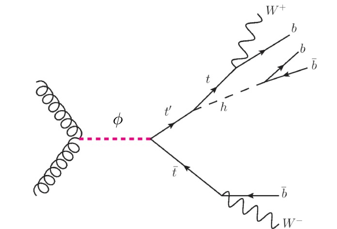
Figure 5: An example of global Higgs produced by gluon fusion and decaying into a top quark and a top partner. The $t^{\prime}$ further decays hadronically, hence the final states are potentially merged.

As is well-known, light enough top partners can be pair-produced via QCD processes, or produced singly, by the fusion of a $W$ and a $b$ quark, in association with a jet and a $b$-jet DeSimone:2012fs ; Azatov:2013hya ; Backovic:2014uma ; Matsedonskyi:2015dns ; Backovic:2015bca . The former process is model-independent while the latter depends on the strength of the coupling $g/\sqrt{2}\,s_{L}\,\bar{t}_{L}^{\prime}W^{\mu}\gamma_{\mu}b_{L}$, where the mixing angle $s_{L}$ vanishes in the absence of EWSB. At the $13$ TeV LHC, single $t^{\prime}$ production is typically expected to dominate over pair production when $m_{t^{\prime}}$ is about a TeV or above. For reference, the production cross-section for a single $t^{\prime}$ of $1$ TeV is approximately

$$\sigma_{t^{\prime}}\approx 4.3\,s_{L}^{2}\,{\rm pb}~{},$$ (30)

at the 14 TeV LHC (using the results in Backovic:2015bca  ). On the other hand, the $t^{\prime}$ mass is constrained by pair production searches at run I ATLAS:2014pga ; Aad:2014efa ; Aad:2015kqa ; Aad:2015gdg ; Chatrchyan:2013uxa ; Khachatryan:2015axa ; CMS:2014rda ; CMS:1900uua ; CMS:2014dka . The $95\%$ lower bound on $m_{t^{\prime}}$ is about $750-900$ GeV depending on the BRs. We shall assume the conservative bound

$$m_{t^{\prime}}>750~{}{\rm GeV}~{}.$$ (31)

The $t^{\prime}$ decays offer several detection channels. The channels with highest branching fraction are the hadronic ones, $t^{\prime}\rightarrow t_{\rm had}Z_{\rm had},\ bW_{\rm had},\ t_{\rm had}h_{\rm had}$. However, these suffer from huge multi-jet, $b\bar{b}+$jets, $t_{\rm had}\rm t_{\rm had}+$jets backgrounds in existing searches focussed on either QCD pair or single $t^{\prime}$ production. Rather refined strategies are often needed to tame the background, involving customized bottom and top tagging, large missing $E_{T}$ cuts, and forward jet tagging. In Ref. Backovic:2015bca , for the case of single $t^{\prime}$ production, the most promising detection channels from each decay mode have been found to be $t_{\rm had}Z_{\rm inv}$, $bW_{\rm lep}$, $t_{\rm had}h_{bb}$. The $t_{\rm had}h_{bb}$ channel requires careful tagging techniques, and the signal drops to $~{}5\%$ after cuts. Given the cross section of Eq. (30), the production rate after cuts may be matched by production via the global Higgs channel that we discuss next.

Compared to the standard $t^{\prime}$ searches, the production of $t^{\prime}\bar{t}^{\prime}$ and $t^{\prime}\bar{t}\,(t\bar{t}^{\prime})$ via decays of the global Higgs presents a number of distinctive features, potentially useful in efficiently eliminating the backgrounds. First, the production is resonant, which is not the case for usual $t^{\prime}$ production modes. The $t^{\prime}\bar{t}^{\prime}$, $t^{\prime}\bar{t}\,(t\bar{t}^{\prime})$ are expected to be produced essentially back-to-back, which provides a constraint on the topology of the event. Resonant production further implies that a shape analysis (i.e. a “bump search”) of the reconstructed $m_{t^{\prime}t^{\prime}}$ ($m_{t^{\prime}t}$) invariant mass can be carried out. Second, in the case of $t^{\prime}\bar{t}$ $(t\bar{t}^{\prime})$ the top is highly boosted typically with $\mathbf{p}_{T}\sim m_{\phi}/2$, so that these events are selected with high trigger efficiency at ATLAS and CMS. Third, if the $t^{\prime}$ is significantly lighter than the global Higgs, the $t^{\prime}$ can be highly boosted. This is in sharp contrast with SM $t^{\prime}$ production, where the $\mathbf{p}_{T}$ of the $t^{\prime}$ is typically small, so that the decay products $th,\ tZ,\ bW^{+}$ are well separated. One may notice that for a boosted $t^{\prime}$, the missing-energy based search in the $tZ_{\rm inv}$ channel proposed in Backovic:2015bca does not work, since the missing-$E_{T}$ from the neutrinos is not resolved anymore. However the high boost also opens up the possibility that the hadronic decay products of the $t^{\prime}$ itself can merge. The object to search for then becomes a single large-radius (i.e. “fat”) $t^{\prime}$-jet. This possibility has, to the best of our knowledge, never been discussed in the literature. Such fat jets should be analyzed using jet substructure techniques. As a basic first step, a grooming technique (filtering BDRS , pruning Ellis:2009su , trimming Krohn:2009th ) can be used to remove extra jets from pileup, soft radiation and the underlying event. The remaining hard subjets can then be used to reconstruct the $t^{\prime}$ 4-momentum. Combining this information with that of the other $t^{\prime}$ or $t$ gives then access to the global Higgs mass itself.

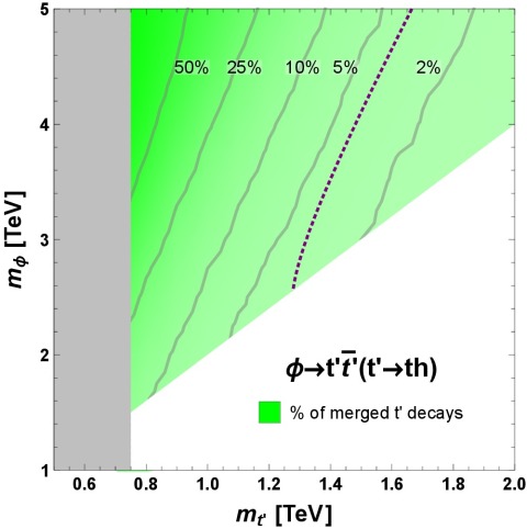
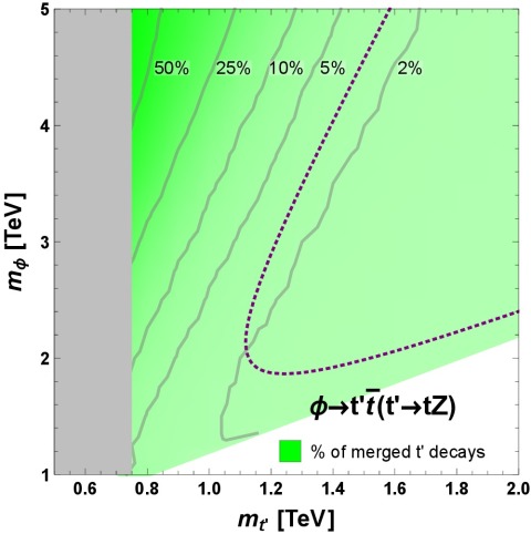
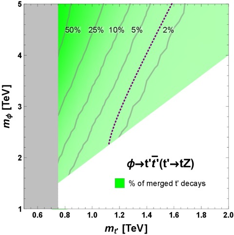
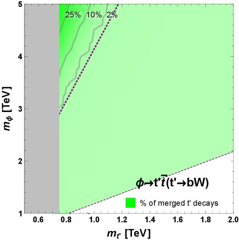
Figure 6: Fraction of merged $t^{\prime}$ decays in the $m_{t^{\prime}}-m_{\phi}$ plane for the cases of $\phi\to t^{\prime}\bar{t}~{}(t\bar{t}^{\prime})$ (left plots) and $\phi\to t^{\prime}\bar{t}^{\prime}$ (right plots). In the white region, these decays cannot occur on-shell. The plots from top to bottom correspond to the possible $t^{\prime}$ decays, $t^{\prime}\to th$, $t^{\prime}\to tZ$ and $t^{\prime}\to bW$. The gray vertical band is a conservative $95\%$ exclusion region from Run I searches. The dashed line is an estimate of the merging region following the calculation of App. B, assuming azimuthal $t^{\prime}$ opening angle (see Eq. (42)).

Let us comment on the possible content of the $t^{\prime}$-jet. The merged decay products from $b+W$ resulting from a boosted $t^{\prime}$ are similar to a hadronic top decay with mass $m_{t}\rightarrow m_{t^{\prime}}$. The merged $t+Z$ decays leads to a fat jet containing $b+2j+2j$, and the merged $t+h$ contains to $b+2j+2b$. These two last decay chains are more likely to produce a fat jet, simply because there are more final states that potentially overlap. Besides, in the $t+h$ channel, tagging the $b$ quarks inside the jet can dramatically reduce the background. This last channel is thus particularly attractive. In order to reduce further the $t^{\prime}$-jet background, tagging techniques can in principle be adapted or developed. Tagging directly the whole $t^{\prime}$ decay seems difficult, since the $t^{\prime}$ mass is a priori unknown and the event has many subjets to combine. A less ambitious approach could be to tag the heavy $W$, $Z$, $h$ and top subjets inside the fat jets. This can be carried out using for example the pruning tagger of Ref. Ellis:2009me . Notice that the uncertainty on the reconstructed subjet masses with this technique is about $\pm 10$ GeV Plehn:2011tg , which implies that the $W$ and $Z$ cannot be distinguished in such an approach.

A boosted $t^{\prime}$-jet is an interesting object, both theoretically as it may signal the existence of the global Higgs, and experimentally as it leads to new channels to be analyzed with dedicated substructure tools. The remaining crucial question is “How likely is it for $t^{\prime}$-jets to be produced from a global Higgs decay?” To answer this, we first notice that for a given production mode of the global Higgs, the fraction of merged $t^{\prime}$ decays depends only on the kinematics of the global Higgs decay chain. Therefore the fraction of merged $t^{\prime}$ decays only depends on the global Higgs mass and the $t^{\prime}$ mass, and can be shown in the $m_{t^{\prime}}-m_{\phi}$ plane irrespective of the details of the model.

We evaluate the fraction of $t^{\prime}$-jets by Monte Carlo (MC) integration. We simulate the process of global Higgs production via ggF using MadGraph5 MG with our implementation of the global Higgs and top partner Lagrangian in FeynRules FR . We analyze the six possible decay chains given by $\phi\rightarrow t^{\prime}\bar{t}~{}(t\bar{t^{\prime}})$, $\phi\rightarrow t^{\prime}\bar{t^{\prime}}$ followed by either $t^{\prime}\rightarrow t_{\rm had}Z_{\rm had},\ bW_{\rm had}$, or $t_{\rm had}h_{bb}$. Denoting schematically $t^{\prime}\rightarrow AB$, the fraction is obtained by requiring that at least one of the jets from $A$ is separated from a jet from $B$ by $\Delta R(A,B)<0.8$. This is done using MadAnalysis5 MA . Using only this condition on $\Delta R(A,B)$ leaves in principle the possibility of having resolved decay products within $A$ or $B$. When this happens, one obtains a “partially-merged” object, which is in principle also interesting. However we checked that in practice, depending on the process under consideration, the fraction of fully-merged events ranges among $\sim 90\%-100\%$. In the following, we do not distinguish between these two subcases and refer to them simply as “merged decays”.

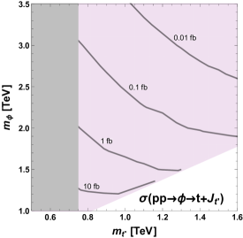
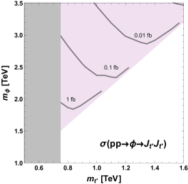
Figure 7: Single and pair production rate of $t^{\prime}$-jets assuming $2:1:1$ branching fractions for the $t^{\prime}\rightarrow bW,tZ$ and $th$ channels. We take $\lambda=0.2$ and assume $100\%$ decays of the global Higgs into $t\bar{t}^{\prime}(t^{\prime}\bar{t})$ (left plot) or into $t^{\prime}\bar{t}^{\prime}$ (right plot).

The fraction of merged $t^{\prime}$ decays in the $m_{t^{\prime}}-m_{\phi}$ plane is shown in Fig. 6. We can see that in case of $t^{\prime}\rightarrow th$ and $tZ$ decays, a sizeable region features more than $10\%$ of $t^{\prime}$-jets. On the other hand, in the case of $bW$ decay, the amount of $t^{\prime}$-jets is smaller by an order of magnitude. This is expected since the $b$ and $W$ jets have a smaller radius than $t$, $Z$, or $h$ jets. These features can also be understood qualitatively using the analytic approach presented in App. B. The fraction of merged $t^{\prime}$ decays obviously increases with $m_{\phi}$ for a fixed $m_{t^{\prime}}$. However, the production rate of the global Higgs drops with $m_{\phi}$. In Fig. 7 we show the expected cross section for $t^{\prime}$-jets, assuming the gluon fusion cross sections estimated in Sec. 3, and using the information of Fig. 6 with branching fractions for $t^{\prime}\to bW$, $t^{\prime}\to tZ$, $t^{\prime}\to th$ in the ratio $2:1:1$. We see that the cross sections are typically small. Nevertheless, it can be interesting to develop methods to detect these novel $t^{\prime}$-jets.

6 Conclusions

In this paper we have performed an investigation of the LHC signatures arising from the global Higgs, the “radial” partner of the NGBs identified as the SM Higgs and EW boson longitudinal polarizations in modern composite Higgs constructions.

We evaluated the LHC sensitivity to global Higgs resonant production. Our results suggest that these global Higgs channels can compete with the standard searches for compositeness via SM production of top partners.

In the case that the global Higgs decays mostly into NGBs and top quarks, and not into fermion resonances, a projection at $300$ fb^-1 of integrated luminosity for boosted hadronic channels gives a sensitivity to the global Higgs up to a mass of $\sim 2.5-3$ TeV. We noted that this case is very predictive, effectively depending on only two parameters $\hat{f}$, $r_{v}$. Measuring both the NGB and $t\bar{t}$ channels would provide an estimation of $r_{v}$. Also, the $WW$, $ZZ$, $hh$ event rates are predicted to be in 2:1:1 proportions.

The case where the global Higgs can decay into fermion resonances is much more model-dependent, hence we focused on a particular (but well-motivated) scenario involving decays into charge $2/3$ top partners. The $t^{\prime}$ produced through such resonant process may in principle be easier to detect than the ones produced by standard SM processes. We also pointed out that in part of the parameter space, such resonantly-produced $t^{\prime}$ can be boosted enough to appear as a single fat jet in the calorimeters. We evaluated by MC simulation the probability of having merged $t^{\prime}$ decay products, and also provided an analytic computation that approximately reproduces the boosted $t^{\prime}$ regions.

Given these first encouraging results, it would be interesting to further investigate the collider implications of the global Higgs. In particular, the rather striking possibility of getting boosted $t^{\prime}$ states requires the development of new, dedicated jet substructure analyses in order to properly select such signatures.

Appendix A Loop Functions

For completeness, we collect here the well-known loop functions (see Djouadi:2005gi , for example) that appear at 1-loop order when considering the couplings of a scalar to gauge bosons via heavy fermion or spin-1 loops:

$$A_{1/2}(\tau) = 2[\tau+(\tau-1)f(\tau)]\tau^{-2}~{},$$ (32)

$$A_{1}(\tau) = -[2\tau^{2}+3\tau+3(2\tau-1)f(\tau)]\tau^{-2}~{},$$ (33)

where

$$f(\tau) = \left\{\begin{array}[]{ll}{\rm arcsin}^{2}\sqrt{\tau}&\tau\leq 1\\[3.99994pt] -\frac{1}{4}\left[\log\frac{1+\sqrt{1-\tau^{-1}}}{1-\sqrt{1-\tau^{-1}}}-i\pi\right]^{2}&\tau>1\end{array}\right.~{}.$$ (36)

In the limit that $\tau\rightarrow 0$, $A_{1/2}(\tau)\rightarrow 4/3$ and $A_{1}(\tau)\rightarrow-7$.

Appendix B An Analytic Estimation of the Boosted $t^{\prime}$ Region

As a complement to the MC simulation above, we provide a purely analytical technique to estimate the boosted $t^{\prime}$ region. Although this approach is only qualitative as it provides only a region and not a density, it has the advantage of being transparent and simple.

We shall first set up some general kinematical expressions related to opening angles of decay products. We consider a particle with mass $m$, arbitrary transverse momentum $p_{T}$ and rapidity $y$ decaying into two particles with transverse momentum $p_{T\,1}$, $p_{T\,2}$, and rapidities $y_{1}$, $y_{2}$, whose masses are neglected with respect to $m$ or $|p_{T}|$. We are interested in the opening angle between the decay products, $(\Delta R)^{2}=(\Delta\eta)^{2}+(\Delta\phi)^{2}$.  An approximation that can be sometimes found in the literature is $\Delta R\approx 2m/|p_{T}|$, which is only valid for $|p_{T}|\gg m$ and for symmetric decay configuration. Here one needs to go beyond this case, so that we revisit the computation in order to establish well-controlled approximate formulas.

Using $p=q_{1}+q_{2}$ with transverse variables, one obtains

$$m^{2}=2|\mathbf{p}_{T\,1}||\mathbf{p}_{T\,2}|(\cosh\Delta y-\cos\Delta\phi)\,,$$ (38)

where $\Delta\phi=\phi_{2}-\phi_{1}$ is the difference between the azimuthal angles and $\Delta y=y_{2}-y_{1}$. In order to go further analytically, an extra condition needs to be chosen. We find that two different conditions independently lead to the same result.

A first condition is to select the particular configuration that gives the minimal $\Delta R$ angle. This lower bound is useful in order to assess the radius for grooming algorithms, and will be needed in our approach to jet merging. Asking for the lowest $\Delta R$ amounts to maximize the $|\mathbf{p_{T\,1}}||\mathbf{p_{T\,2}}|$ product. Using transverse momentum conservation, one obtains that

$$|\mathbf{p}_{T\,1}|=|\mathbf{p}_{T\,2}|=\frac{|\mathbf{p_{T}}|}{2\cos(\Delta\phi/2)}\,.$$ (39)

Using this expression in Eq. (38) provides the main formula

$$\frac{\cos^{2}(\Delta\phi/2)}{\cosh^{2}(\Delta y/2)}=\frac{|\mathbf{p}_{T}|^{2}}{m^{2}+|\mathbf{p}_{T}|^{2}}\,.$$ (40)

Alternatively, this equation can also be obtained starting from the condition $|\mathbf{p_{T\,1}}|=|\mathbf{p_{T\,2}}|$, which is motivated by the fact that such symmetric configuration is statistically the most likely to occur in the two-body decay. Together with momentum conservation, the condition implies that $y=(y_{1}+y_{2})/2$ exactly, and Eq. (40) follows. This equation provides the kinematic bounds on $\Delta\phi$, $\Delta y$. From (39), one can see that the minimal and maximal $|\mathbf{p}_{T\,1,2}|$ are respectively equal to $|\mathbf{p}_{T}|/2$, $\sqrt{m^{2}+|\mathbf{p}_{T}|^{2}}/2$, and correspond respectively to $\Delta\phi=0$ and $\Delta y=0$.

The only assumption done at this stage is on the absolute value of outgoing transverse momenta. Assuming further that $\Delta\phi\ll 1$ and $\Delta y\ll 1$, Eq. (40) implies that $m\ll|\mathbf{p}_{T}|$ and it then follows that

$$\Delta R=\frac{2m}{{|\mathbf{p}_{T}|}}+O\left(\Delta y^{4},\Delta\phi^{4}\right)\,.$$ (41)

which is the usual approximation.

When $\Delta R$ is not small with respect to one, Eq. (41) is not valid anymore. One can rather consider the particular cases $\Delta y\ll\Delta\phi\approx\Delta R$ and $\Delta\phi\ll\Delta y\approx\Delta R$, which give respectively

$$\Delta R=2\,\arctan\left(\frac{m}{|\mathbf{p}_{T}|}\right)+O(\Delta y^{2})\,,$$ (42)

$$\Delta R=2\,\operatorname{arcsinh}\left(\frac{m}{|\mathbf{p}_{T}|}\right)+O(\Delta\phi^{2})\,.$$ (43)

These approximations will be used in our approach to jet merging.

Finally, it is also necessary to consider configurations giving an upper bound on $\Delta R$. These arise from decays with asymmetric transverse momentum. A sensible condition on the asymmetry is the one given by the experimental jet definition. We use the standard asymmetry measure BDRS

$$\tau=\frac{\min(|\mathbf{p}_{T\,1}|^{2},|\mathbf{p}_{T\,2}|^{2})}{m^{2}}\Delta R^{2}\,.$$ (44)

Below a threshold $\tau_{\rm cut}$, the jet is considered to be too asymmetric to be likely to arise from the decay of a massive particle. We write $|\mathbf{p}_{T,2}|=a|\mathbf{p}_{T,1}|$, choosing $a>1$ without loss of generality. Assuming $\Delta\phi\ll\Delta y$, one gets

$$\Delta R=2\,{\rm arcsinh}\left(\frac{m}{2|\mathbf{p}_{T}|}\frac{1+a}{\sqrt{a}}\right)+O\left(\Delta\phi^{2}\right)\,.$$ (45)

Combining the asymmetry threshold $\tau\equiv\tau_{\rm cut}$ and Eqs. (44), (45), one gets the threshold value $a_{\rm cut}$. This is $a_{\rm cut}=1/\tau_{\rm cut}$ in the small angle limit, i.e. $a\gg 1$, and has to be obtained numerically if this condition is not fulfilled. This provides the upper bound $\Delta R_{\rm cut}=\Delta R(a=a_{\rm cut})$ which is used in Sec. 5.

We can now use these expressions to estimate the region where $t^{\prime}$ fat jets are likely to occur. Clearly, $t^{\prime}$ decays tend to be more collimated at high $\mathbf{p}_{T}$. However, a subtlety is that the subsequent $t,h,Z$ and $W$ jets should also get more collimated as they inherit a higher $\mathbf{p}_{T}$ from the mother particle. Our strategy is to look for the most favorable phase space configuration. If this configuration does not lead to jet merging, then the $t^{\prime}$ decays are resolved over the whole phase space. This most favorable configuration is for a $t^{\prime}$ decaying at minimal $\Delta R$ and at zero rapidity, and for daughter particles decaying at maximal $\Delta R$ as determined by the asymmetry cut. The opening angle for the $t^{\prime}$ decay is given by Eqs. (42), (43). The daughters (i.e. $t$, $h$, $W$, $Z$) decay asymmetrically with $\Delta R$ given by Eq. (45), using the standard cut $\tau_{\rm cut}=0.09$.

The condition for two jets $1,2$ arising from a same vertex to be resolved is

$$\Delta R_{12}\leq R_{1}+R_{2}\,.$$ (46)

When this condition is not fulfilled, the radius of the single jet formed by the two merging jets is

$$R=\max\left[R_{1},R_{2},\frac{\Delta R_{12}+R_{1}+R_{2}}{2}\right]\,.$$ (47)

Applied to the $t^{\prime}$ decay, the condition Eq. (46) determines whether the $t^{\prime}$ decay products are resolved. The radius of the $t,h,Z,W$ jets is described by Eq. (47). Finally, we also need the $t^{\prime}$ transverse momentum at zero rapidity. This is a function of the global Higgs and $t^{\prime}$ masses, given by

$$|\mathbf{p}_{T}|_{t^{\prime}} = \frac{1}{2}\sqrt{m_{\phi}^{2}-4m_{t^{\prime}}^{2}}\,\quad\textrm{for}\quad\phi\rightarrow t^{\prime}\bar{t}\,(t\bar{t}^{\prime})\,,$$ (48)

$$|\mathbf{p}_{T}|_{t^{\prime}} = \frac{1}{2}\left(m_{\phi}-\frac{m_{t^{\prime}}^{2}}{m_{\phi}}\right)\,\quad\textrm{for}\quad\phi\rightarrow t^{\prime}\bar{t}^{\prime}\,,$$ (49)

when the top mass is neglected.

Putting all these pieces together provides a region of the parameter space where $t^{\prime}$-jets can potentially occur. This region is displayed for every decay in Fig. 6. For the asymmetry criteria $\tau_{\rm cut}=0.09$, it turns out this matches roughly the region with a fraction of $2-5\%$ of $t^{\prime}$-jets. The region obtained in case of azimuthal $t^{\prime}$ decay configuration Eq. (42) turns out to be larger than for polar decay Eq. (43), so that we display only the former.

References

- (1) D. Buttazzo, F. Sala, and A. Tesi, Singlet-like Higgs bosons at present and future colliders, JHEP 11 (2015) 158, [arXiv:1505.05488].
- (2) F. Feruglio, B. Gavela, K. Kanshin, P. A. N. Machado, S. Rigolin, and S. Saa, The minimal linear sigma model for the Goldstone Higgs, JHEP 06 (2016) 038, [arXiv:1603.05668].
- (3) S. Fichet, G. von Gersdorff, E. Pontón, and R. Rosenfeld, The Excitation of the Global Symmetry-Breaking Vacuum in Composite Higgs Models, arXiv:1607.03125.
- (4) ATLAS Collaboration, G. Aad et al., Observation of a new particle in the search for the Standard Model Higgs boson with the ATLAS detector at the LHC, Phys. Lett. B716 (2012) 1–29, [arXiv:1207.7214].
- (5) CMS Collaboration, S. Chatrchyan et al., Observation of a new boson at a mass of 125 GeV with the CMS experiment at the LHC, Phys. Lett. B716 (2012) 30–61, [arXiv:1207.7235].
- (6) G. von Gersdorff, E. Pontón, and R. Rosenfeld, The Dynamical Composite Higgs, JHEP 06 (2015) 119, [arXiv:1502.07340].
- (7) A. Djouadi, The Anatomy of electro-weak symmetry breaking. I: The Higgs boson in the standard model, Phys. Rept. 457 (2008) 1–216, [hep-ph/0503172].
- (8) G. Panico and A. Wulzer, The Composite Nambu-Goldstone Higgs, Lect. Notes Phys. 913 (2016) pp.1–316, [arXiv:1506.01961].
- (9) ATLAS Collaboration Collaboration, Measurements of the properties of the Higgs-like boson in the four lepton decay channel with the ATLAS detector using 25 fb−1 of proton-proton collision data, Tech. Rep. ATLAS-CONF-2013-013, CERN, Geneva, Mar, 2013.
- (10) J. Alwall, R. Frederix, S. Frixione, V. Hirschi, F. Maltoni, O. Mattelaer, H. S. Shao, T. Stelzer, P. Torrielli, and M. Zaro, The automated computation of tree-level and next-to-leading order differential cross sections, and their matching to parton shower simulations, JHEP 07 (2014) 079, [arXiv:1405.0301].
- (11) A. Alloul, N. D. Christensen, C. Degrande, C. Duhr, and B. Fuks, FeynRules 2.0 - A complete toolbox for tree-level phenomenology, Comput. Phys. Commun. 185 (2014) 2250–2300, [arXiv:1310.1921].
- (12) NNPDF Collaboration, R. D. Ball, V. Bertone, S. Carrazza, L. Del Debbio, S. Forte, A. Guffanti, N. P. Hartland, and J. Rojo, Parton distributions with QED corrections, Nucl. Phys. B877 (2013) 290–320, [arXiv:1308.0598].
- (13) A. Carmona, A. Delgado, M. Quirós, and J. Santiago, Diboson resonant production in non-custodial composite Higgs models, JHEP 09 (2015) 186, [arXiv:1507.01914].
- (14) ATLAS Collaboration, G. Aad et al., Search for Higgs boson pair production in the final state from pp collisions at TeVwith the ATLAS detector, Eur. Phys. J. C75 (2015), no. 9 412, [arXiv:1506.00285].
- (15) J. M. Butterworth, A. R. Davison, M. Rubin, and G. P. Salam, Jet substructure as a new Higgs search channel at the LHC, Phys. Rev. Lett. 100 (2008) 242001, [arXiv:0802.2470].
- (16) ATLAS Collaboration, G. Aad et al., Search for high-mass diboson resonances with boson-tagged jets in proton-proton collisions at = 8 TeV with the ATLAS detector, arXiv:1506.00962.
- (17) S. Fichet and G. von Gersdorff, Effective theory for neutral resonances and a statistical dissection of the ATLAS diboson excess, arXiv:1508.04814.
- (18) B. C. Allanach, B. Gripaios, and D. Sutherland, Anatomy of the ATLAS diboson anomaly, Phys. Rev. D92 (2015), no. 5 055003, [arXiv:1507.01638].
- (19) J. Stirling. LHC cross-section plots available on http://www.hep.ph.ic.ac.uk/ wstirlin/plots/plots.html).
- (20) D. Goncalves, F. Krauss, and M. Spannowsky, Augmenting the diboson excess for the LHC Run II, Phys. Rev. D92 (2015), no. 5 053010, [arXiv:1508.04162].
- (21) J. O. Berger and T. Sellke, Testing a Point Null Hypothesis: The Irreconcilability of P Values and Evidence, J. Am.Stat. Assoc. 82 (1987) No. 397, pp. 112–122.
- (22) J. O. Berger, M. J. Bayari, and T. Sellke, Calibration of p Values for Testing Precise Null Hypotheses, The American Statistician (2001) 55:1, 62–71.
- (23) G. Cowan, K. Cranmer, E. Gross, and O. Vitells, Asymptotic formulae for likelihood-based tests of new physics, Eur. Phys. J. C71 (2011) 1554, [arXiv:1007.1727]. [Erratum: Eur. Phys. J.C73,2501(2013)].
- (24) Search for heavy particles decaying to pairs of highly-boosted top quarks using lepton-plus-jets events in proton–proton collisions at TeV with the ATLAS detector, Tech. Rep. ATLAS-CONF-2016-014, CERN, Geneva, Mar, 2016.
- (25) M. Backovic, T. Flacke, J. H. Kim, and S. J. Lee, Search Strategies for TeV Scale Fermionic Top Partners with Charge 2/3, JHEP 04 (2016) 014, [arXiv:1507.06568].
- (26) M. Backović, T. Flacke, S. J. Lee, and G. Perez, LHC Top Partner Searches Beyond the 2 TeV Mass Region, JHEP 09 (2015) 022, [arXiv:1409.0409].
- (27) A. De Simone, O. Matsedonskyi, R. Rattazzi, and A. Wulzer, A First Top Partner Hunter’s Guide, JHEP 04 (2013) 004, [arXiv:1211.5663].
- (28) A. Azatov, M. Salvarezza, M. Son, and M. Spannowsky, Boosting Top Partner Searches in Composite Higgs Models, Phys. Rev. D89 (2014), no. 7 075001, [arXiv:1308.6601].
- (29) O. Matsedonskyi, G. Panico, and A. Wulzer, Top Partners Searches and Composite Higgs Models, JHEP 04 (2016) 003, [arXiv:1512.04356].
- (30) ATLAS Collaboration, T. A. collaboration, Search for pair and single production of new heavy quarks that decay to a boson and a third generation quark in collisions at TeV with the ATLAS detector, .
- (31) ATLAS Collaboration, G. Aad et al., Search for pair and single production of new heavy quarks that decay to a boson and a third-generation quark in collisions at TeV with the ATLAS detector, JHEP 11 (2014) 104, [arXiv:1409.5500].
- (32) ATLAS Collaboration, G. Aad et al., Search for production of vector-like quark pairs and of four top quarks in the lepton-plus-jets final state in collisions at TeV with the ATLAS detector, JHEP 08 (2015) 105, [arXiv:1505.04306].
- (33) ATLAS Collaboration, G. Aad et al., Analysis of events with -jets and a pair of leptons of the same charge in collisions at TeV with the ATLAS detector, JHEP 10 (2015) 150, [arXiv:1504.04605].
- (34) CMS Collaboration, S. Chatrchyan et al., Inclusive search for a vector-like T quark with charge in pp collisions at = 8 TeV, Phys. Lett. B729 (2014) 149–171, [arXiv:1311.7667].
- (35) CMS Collaboration, V. Khachatryan et al., Search for vector-like T quarks decaying to top quarks and Higgs bosons in the all-hadronic channel using jet substructure, JHEP 06 (2015) 080, [arXiv:1503.01952].
- (36) CMS Collaboration, C. Collaboration, Search for vector-like top quark partners produced in association with Higgs bosons in the diphoton final state, .
- (37) CMS Collaboration, C. Collaboration, Search for pair-produced vector-like top quark partners decaying to bW in the fully hadronic channel using jet substructure at 8 TeV, .
- (38) CMS Collaboration, C. Collaboration, Search for vector-like quarks in final states with a single lepton and jets in pp collisions at sqrt s = 8 TeV, .
- (39) J. M. Butterworth, A. R. Davison, M. Rubin, and G. P. Salam, Jet substructure as a new Higgs search channel at the LHC, Phys. Rev. Lett. 100 (2008) 242001, [arXiv:0802.2470].
- (40) S. D. Ellis, C. K. Vermilion, and J. R. Walsh, Techniques for improved heavy particle searches with jet substructure, Phys. Rev. D80 (2009) 051501, [arXiv:0903.5081].
- (41) D. Krohn, J. Thaler, and L.-T. Wang, Jet Trimming, JHEP 02 (2010) 084, [arXiv:0912.1342].
- (42) S. D. Ellis, C. K. Vermilion, and J. R. Walsh, Recombination Algorithms and Jet Substructure: Pruning as a Tool for Heavy Particle Searches, Phys. Rev. D81 (2010) 094023, [arXiv:0912.0033].
- (43) T. Plehn and M. Spannowsky, Top Tagging, J. Phys. G39 (2012) 083001, [arXiv:1112.4441].
- (44) E. Conte, B. Fuks, and G. Serret, MadAnalysis 5, A User-Friendly Framework for Collider Phenomenology, Comput. Phys. Commun. 184 (2013) 222–256, [arXiv:1206.1599].
- (45) ATLAS, CMS Collaboration, M. Negrini, Review of physics results using jet substructure techniques in LHC Run1, EPJ Web Conf. 90 (2015) 09001.