Human collective intelligence as distributed Bayesian inference

Abstract

Collective intelligence is believed to underly the remarkable success of human society. The formation of accurate shared beliefs is one of the key components of human collective intelligence. How are accurate shared beliefs formed in groups of fallible individuals? Answering this question requires a multiscale analysis. We must understand both the individual decision mechanisms people use, and the properties and dynamics of those mechanisms in the aggregate. As of yet, mathematical tools for such an approach have been lacking. To address this gap, we introduce a new analytical framework: We propose that groups arrive at accurate shared beliefs via distributed Bayesian inference. Distributed inference occurs through information processing at the individual level, and yields rational belief formation at the group level. We instantiate this framework in a new model of human social decision-making, which we validate using a dataset we collected of over 50,000 users of an online social trading platform where investors mimic each others’ trades using real money in foreign exchange and other asset markets. We find that in this setting people use a decision mechanism in which popularity is treated as a prior distribution for which decisions are best to make. This mechanism is boundedly rational at the individual level, but we prove that in the aggregate implements a type of approximate “Thompson sampling”—a well-known and highly effective single-agent Bayesian machine learning algorithm for sequential decision-making. The perspective of distributed Bayesian inference therefore reveals how collective rationality emerges from the boundedly rational decision mechanisms people use.

Human groups have an incredible capacity for technological, scientific, and cultural creativity. Our historical accomplishments and the opportunity of modern networked society to stimulate ever larger-scale collaboration have spurred broad interest in understanding the problem-solving abilities of groups—their collective intelligence. The phenomenon of collective intelligence has now been studied extensively across animal species [1]; collective intelligence has been argued to exist as a phenomenon distinct from individual intelligence in small human groups [2]; and the remarkable abilities of large human collectives have been extensively documented [3]. However, while the work in this area has catalogued what groups can do, and in some cases the mechanisms behind how they do it, we still lack a coherent formal perspective on what human collective intelligence actually is. There is a growing view of group behavior as implementing distributed algorithms [4, 5, 6, 7], which goes a step beyond the predominant analytical framework of agent-based models in that it formalizes specific information processing tasks that groups are solving. Yet this perspective provides little insight into one of the key features of human group cognition—the formation of shared beliefs [8, 9, 10, 11, 12, 13].

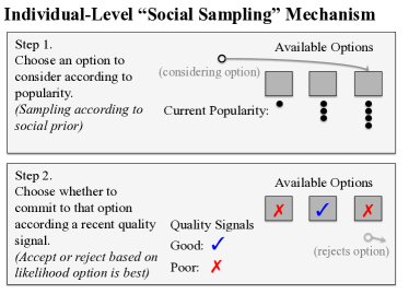
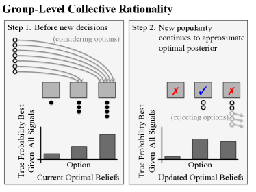
Figure 1: A schematic illustration of the “social sampling” mechanism we propose as a model of human social decision-making, and an illustration of how this mechanism yields collectively rational belief formation at the group level. Individuals treat current popularity as a prior distribution, and sample according to this prior in order to choose an option to consider taking. An individual then commits to a considered option with probability proportional to the likelihood that the option is best given a recent objective signal of quality. If current popularity approximates the current optimal posterior distribution that each option is best given all previous quality signals, then when a large group of decision-makers continues to use the social sampling mechanism, popularity will continue to approximate the optimal posterior.

Recent work in cognitive science has provided a way to understand belief formation at the level of individual intelligence. One productive framework treats people as approximately Bayesian agents with rich mental models of the world [14, 15]. Beliefs that individuals hold are viewed as posterior distributions, or samples from these distributions, and the content and structure of those beliefs come from the structure of people’s mental models as well as their objective observations. Belief formation is viewed as approximate Bayesian updating, conditioning these mental models on an individual’s observations. We propose to model human collective intelligence as distributed Bayesian inference, and we present the first empirical evidence for such a model from a large behavioral dataset. Our model shows how shared beliefs of groups can be formed at the individual level through interactions with others and private boundedly rational Bayesian updating, while in aggregate implementing a rational Bayesian inference procedure.

We instantiate this broader framework in the context of social decision-making. A social decision-making problem represents a setting in which a group of people makes decisions among a shared set of options, and previous decisions are public. Examples of social decision-making problems include choosing what restaurant to visit using a social recommendation system, choosing how to invest your money after reading the news, or choosing what political candidate to support after talking with your friends. We instantiate our framework of collective intelligence as distributed Bayesian inference in a new mathematical model of human social decision-making, and then we evaluate this model quantitatively with a unique large-scale social decision-making dataset that allows us to test the model’s predictions in ways previous datasets have not enabled.

Our model, illustrated in Figure 1, posits that individuals first choose options to consider based on popularity, then choose to commit to those options based on assessments of objective evidence. A Bayesian interpretation of this strategy suggests that people are trying to infer the best decisions to make by treating popularity as a prior distribution that summarizes past evidence. A large group of people using this strategy will collectively perform rational inferences. We test this model, and thereby test our broader framework, by showing the model is able to account for the patterns of social influence we observe in our data better than several alternatives.

Formally, we propose that a person in a social decision-making context will first choose an option $j$ to consider with probability proportional to its current popularity at time $t$, $p_{j,t}$. The decision-maker then evaluates the quality of that option using a recent performance signal $r_{j,t}$, which for simplicity we assume indicates either good quality ($r_{j,t}=1$) or poor quality ($r_{j,t}=0$). The decision-maker then chooses to commit to that option with probability $\eta>0.5$ if the signal is good or $1-\eta$ if the signal is bad (where $\eta$ is a free parameter). The probability that a decision-maker commits to option $j$ at time $t$ is then

$$\frac{p_{j,t}\eta^{r_{j,t}}(1-\eta)^{1-r_{j,t}}}{\sum_{k}p_{k,t}\eta^{r_{k,t}}(1-\eta)^{1-r_{k,t}}}.$$ (1)

We call this decision-making strategy “social sampling”. Heuristics similar to the social sampling model have been previously proposed [16, 17, 18, 19, 20, 21, 22]. In particular, two-stage social decision-making models appear to be common across animal species [23, 24]. The social sampling model is also mathematically equivalent to a novel kind of stochastic actor-oriented model [25], and is related to a number of other prior models of social learning and social influence [26, 27, 28, 29, 30]. However, our treatment is substantially different from these previous accounts. The specific mathematical form of this model, which in its details is distinct from any previously proposed, has a boundedly rational cognitive interpretation at the individual level, and affords a coherent cognitive interpretation at the group level. We can thus establish a formal relationship between individual behavior, individual cognition, and expressed collective belief.

From the perspective of an individual decision-maker, there is a simple Bayesian cognitive analysis [15] that explains the mathematical form of Equation (1). Equation (1) can be interpreted as the posterior probability that option $j$ is the best option available if the mental model people have is that (a) there is a single best option (a needle in the haystack) producing good signals with probability $\eta$ while all other options produce good and bad signals with equal probability, and (b) the market share of option $j$, $\frac{p_{j}}{\sum_{k}p_{k}}$, corresponds to the prior probability that $j$ is the best option. (See Section “Social Sampling Model Specification” in the appendix for additional details.) Assuming that popularity is a reasonable proxy for prior probability, choosing option $j$ with the probability given by Equation (1), i.e. “probability matching” on this posterior, can be viewed as rational under certain resource constraints [31, 32]. Social sampling is therefore a boundedly rational probabilistic decision-making strategy that is far more computationally efficient than exhaustive search over all options.

Taking into consideration the behavior of an entire group that uses social sampling, we can also prove that it is rational for decision-makers to treat popularity as a prior distribution in this way. When the entirety of a population uses this strategy, the expected new popularity of each option $p_{j,t^{\prime}}$ will be proportional to the previous posterior probability that the option was best. Popularity will then come to approximate a rational prior in the steady-state dynamics of a large population all participating in social sampling. Social sampling becomes “collectively rational” for this reason. Optimal posterior inferences arise from a calibrated social prior represented at the group level being combined with new evidence obtained by the group members. The group therefore collectively transforms a boundedly rational heuristic at the individual level into a distributed implementation of a fully Bayesian inference procedure at the group level. In light of the Bayesian perspective of cognition, the collective rationality of social sampling shows how groups can be interpreted as irreducible, cognitively coherent, distributed information processing systems.

Results

To test the social sampling model, we make use of a unique observational dataset from a large online financial trading platform called “eToro”. eToro’s platform allows users to invest real money in foreign exchange markets and other asset markets, and also allows its users to mimic each other’s trades. When a trader becomes a “mimicker” of a target user, the mimicking trader allocates a fixed amount of funds to automatically mirror the trades that the target user makes. The number of mimickers a user has represents the popularity of the decision to mimic that user, and the user’s trading performance indicates the quality of the decision to mimic that user. We treat the decision of whom to mimic on eToro as a social decision-making problem. The dataset we use consists of a year of trading activity from 57,455 users of eToro’s online social trading platform [33]. The website includes search and profile functionality that display both popularity and performance information of the users on the site. For our analysis, we summarize each user’s trading performance with expected return on investment (ROI) from closed trades over a 30-day rolling window, which is similar to the performance metrics presented to the site’s users.

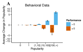
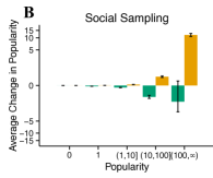
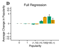
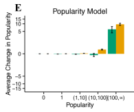
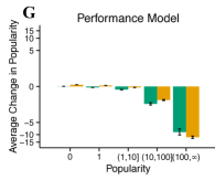
Figure 2: (A) Observational evidence for the multiplicative interaction between popularity and performance in determining future popularity predicted by the social sampling model. (Interaction term $p=0.012$ in a linear model with fixed effects for users and days, and Arellano robust standard errors [34] to adjust for non-equal variance and correlated error terms.) Error bars are 95% Gaussian confidence intervals of the means. (B-G) Replications of Panel A using predicted gains in mimickers according to each model considered, with losses in mimickers taken from the behavioral data. To generate the predictions of each model, we compute the expected number of new mimickers each user gets on each day given the actual total number of new mimic decisions. The social sampling model provides a better fit to our data than all the alternative models.

One striking fact apparent in this dataset is that users are more likely to mimic popular traders, but only if those traders are performing well. While traders on eToro always tend to gain mimickers when they are performing well and lose mimickers when they are performing poorly, the magnitudes of these changes are larger when a trader is more popular. More specifically, we see that daily changes in popularity for each user are predicted by a multiplicative interaction between the past day’s performance and popularity (Figure 2A). People therefore rely heavily on social information even in the presence of explicit, public signals about which traders perform best.

The social sampling model reproduces the multiplicative interaction between popularity and performance that we observe in our data (Figure 2B). The predictions of the social sampling model also compare favorably to five alternative models that were chosen to represent the predictions of simple heuristic and purely rational models of social decision-making, as well as other plausible alternatives (see Section “Model Comparison” in the appendix for further model comparisons). None of these alternatives reproduces the qualitative form of the popularity-performance interaction (Figures 2C through 2G). Models relying too heavily on social information overestimate the increases in popularity of already-popular users (Figures 2E and 2F), and models relying too heavily on performance underestimate those increases (Figures 2C and 2G).

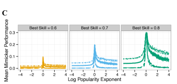
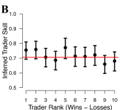
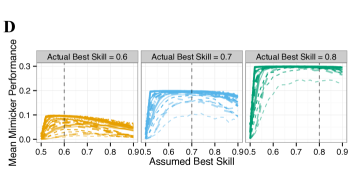
Figure 3: Further evidence from our data for the specific mathematical form of the social sampling model, and evidence from simulations for how the social sampling model yields collectively rational shared belief formation. (A) Log likelihood values for alternative scaling exponents on popularity in the social sampling model. The vertical line indicates the maximum. A log popularity exponent of 0, which corresponds to using popularity linearly as in the social sampling model, achieves the best fit. (B) 95% credible intervals for how often each of the ten best traders in our dataset has positive daily return. The horizontal red line indicates the model’s inferred $\eta$ parameter. The fact that this line passes through all of the credible intervals indicates that the fitted model independently captures this property of the data. (C-D) Two idealized simulation experiments. Each line represents a different combination of simulation parameters, with the four graphical parameters of the plotted lines (line type, width, color, and transparency) each representing a variable. An “assumed best skill” value of 0.5 corresponds to decision-makers ignoring performance information. The fact that group performance peaks at 0 in Panel C indicates that using popularity linearly, as in the social sampling model, is critical to collective rationality. At the same time, the flatness of the curves in Panel D indicates that social sampling is otherwise robust to deviations in individuals’ mental models of the world.

The Bayesian interpretation of social sampling is also supported by specific quantitative features of our data. Rather than using popularity directly as a prior, as in social sampling, individuals could hypothetically form a prior based on a superlinear or sublinear transformation of popularity, $(p_{k})^{\gamma}$. Figure 3A shows that using popularity linearly ($\gamma=1$) is a better fit to our data. We also find that the empirically best fitting value of the social sampling model’s $\eta$ parameter is consistent with the parameter’s Bayesian interpretation. The fitted value of $\eta$ matches what could independently be expected to be the highest frequency of good performance signals from any trader in our dataset, even though the parameter is inferred from users’ mimic decisions and not directly from performance information (Figure 3B).

But why might a group of individuals use social sampling? We have already explained how social sampling in the aggregate yields rational individual posterior-matched decisions. Here we note that the rational mechanism that social sampling collectively implements closely approximates a well-known single-agent algorithm called “Thompson sampling”. Thompson sampling is a Bayesian algorithm for sequential decision-making that consists of probability matching on the posterior probability that an option is best at each point in time. Thompson sampling has been shown in the single-agent case to have state-of-the-art empirical performance and strong optimality guarantees in sequential decision-making problems [35]. As long as popularity remains well-calibrated, social sampling therefore collectively attains these benefits while avoiding the need for any agent to incur the cost of computing a full posterior distribution.

Furthermore, we find that social sampling has unique benefits to group performance compared to nearby models that do not yield a Bayesian algorithm in the aggregate. Firstly, using popularity linearly is critical for the collective rationality of social sampling: it provides dramatically better group outcomes as compared to even small deviations from linearity (Figure 3C). Hence the identification of popularity with a Bayesian prior in individuals’ “posterior matched” choices appears to be necessary for information from individual decisions to accumulate at the group level in a collectively rational fashion. Further simulations also indicate that incorporating performance information into decision-making is normatively vastly better than ignoring it, though the specific value of the $\eta$ parameter is not critical (Figure 3D). This result suggests that the benefits of social sampling may be robust to a group having an inaccurate mental model of the world, at least as long as individuals in the group are making their decisions according to some reasonable shared mental model. Having a shared mental model allows information to accumulate in a Bayesian fashion, while having an inaccurate model appears to only lead to mild inefficiencies.

Discussion

These findings support our view of collective intelligence as distributed Bayesian inference. The more general utility of this framework will come from providing a principled constraint on individual-level mechanisms in modeling collective behavior, and from providing a rigorous way to relate these individual-level mechanisms to group-level models. Looking to the literatures on computer science, statistics, and signal processing for relevant distributed inference algorithms is likely to yield a fruitful path towards a new class of models of human collective behavior. At the same time, instances of this new class of models, such as our social sampling model, will bring novel algorithms to the area of distributed Bayesian inference.

Materials and Methods

Data Processing

The dataset provided to us by eToro consists of a set of trades from the eToro website. The aggregated data we used in our analyses will be released upon publication. The entire dataset contains trades that were closed between June 1, 2011 and November 21, 2013. Our initial explorations (which multiple authors engaged in) must be assumed to have touched all of the data. When we began systematic analysis, in order to have a held-out confirmatory validation set for this analysis, we split the dataset into two years. We use the first year of data for all our main analysis. We then verify that our findings from these analyses still hold in the second year. The second year was almost completely held out after this point, but did witness at least one major model iteration that was primarily motivated by theoretical considerations and a lack of fit of a previous model on the first year of data. Ultimately, the results on the second year of data are similar to those on the first year, with the most notable differences being that the alternative model that relies on social information alone has more competitive predictive performance on the second year. We also test the robustness of our main analysis to the specification of the performance metric we use and the way we parsed our raw data, and we find that our results are highly robust to these changes. (See Sections “Data Processing” and “Robustness Checks” in the appendix for further details on data processing and robustness analysis.)

Predicting Mimic Decisions

Our analysis relied on computing the mimic decisions users on eToro would have been expected to have made according to the social sampling model and alternative models. In all cases we examine aggregations of these decisions in the form of predicting the total number of new mimickers each trader on eToro obtains. More specifically, we predict the number of new mimickers each user gets on each day given the performance and popularity of that user (and of every other user) on the previous day, and given the total number of new mimic events we observe on those days.

In the social sampling model, decision-makers make decisions independently, so the probability that a given decision-maker chooses a specific option $j$ at time $t$ is given by the decision probability $\theta^{main}_{j,t}$,

$$\theta^{main}_{j,t}=\frac{\eta^{r_{j,t}}(1-\eta)^{1-r_{j,t}}\cdot(p_{j,t}+\epsilon_{t})}{\sum_{k}\eta^{r_{k,t}}(1-\eta)^{1-r_{k,t}}\cdot(p_{k,t}+\epsilon_{t})},$$

where $\epsilon_{t}>0$ is a small smoothing parameter that ensures all users have some probability of gaining mimickers, and $r_{j,t}$ in the case of the eToro data simply indicates whether user $j$ has positive or negative performance on day $t$. We arbitrarily choose $\epsilon_{t}=\frac{1}{M_{t}}$, where $M_{t}$ is the number of active users on day $t$. The distribution of the number of new mimickers each user gets on day $t$ will then be given by a multinomial distribution over the $M_{t}$ options with parameters equal to the total number of new mimickers on that day and the vector of probabilities $[\theta^{main}_{1,t},\ldots,\theta^{main}_{M_{t},t}]$. Hence the expected number of new mimickers a particular user $j$ gets on a particular day $t$ will be $\theta^{main}_{j,t}$ times the total number of new mimickers on that day.

Alternative Models

We consider a set of alternative models in order to identify how well the social sampling model is able to account for structure in the mimic decisions present in our data compared to alternative plausible models. We specify these alternative models in terms of “decision probabilities” analogous to $\theta^{main}_{j,t}$. These decision probabilities provide the probability under each model that an individual will decide to commit to a particular option (or mimic a particular trader in the case of eToro). It is possible to specify all our alternative models in this way because every model we consider assumes that all decisions are conditionally independent given the popularity and performance of every option.

The first of these alternatives is a proxy for a probability matching rational agent model that we call the “Performance Regression” model. This model uses only performance information, and does not reduce the performance signals to being binary as our social sampling model does. The decision probability under this model is

$$\theta^{perf}_{j,t}\propto\sigma(\beta_{0}+\beta_{1}q_{j,t}),$$

where $\sigma$ is the logistic function and the $\beta_{i}$ variables are free parameters. In combination with our explorations of different performance metrics (described in Section “Robustness Checks” of the appendix), the performance regression allows us to evaluate the predictive power of using performance information alone to predict mimic decisions.

The next alternative we consider is an extended regression model that we call the “Full Regression” model. This alternative consists of a generalized linear model that includes an interaction term between popularity and performance. Such a model could conceivably generate the multiplicative interaction effects we observe in the eToro data, but lacks some of the additional structure that the social sampling model has. The full regression assumes that a decision-maker chooses to commit to option $j$ with probability

$$\theta^{full}_{j,t}\propto\sigma(\beta_{0}+\beta_{1}q_{j,t}+\beta_{2}p_{j,t}+\beta_{3}q_{j,t}p_{j,t}),$$

where the notation is as above. The purpose of comparing to this alternative is to test whether having the additional structure of including popularity as a prior in the social sampling model lends additional predictive power, as compared to having a heuristic combination of popularity and performance.

We also consider a reduction of the social sampling model that does not use performance information. We call this model the “Popularity Model”. Under the popularity model the decision probability becomes

$$\theta^{pop}_{j,t}\propto p_{j,t}+\epsilon_{t},$$

and again we use $\epsilon_{t}=\frac{1}{M_{t}}$ as the smoothing parameter. Comparing to this preferential attachment model allows us to understand how much predictive power we get from including performance information while controlling for the structure of how social information is used in the social sampling model. This preferential attachment model is a canonical simple heuristic model of social decision-making.

We also consider an alternative model that is a reduction of the social sampling model that uses only performance information. This model, which we refer to as the “Performance Model”, uses the decision probability

$$\theta^{perfm}_{j,t}\propto\eta^{r_{j,t}}(1-\eta)^{1-r_{j,t}}.$$

Since the performance model is the one that would be obtained from the social sampling model when all options have the same popularity, this model allows us to predict how decision-makers might behave if they did not have social information.

Our final alternative model is an additive combination of the popularity model and the performance model. This model, which we call the “Additive Model”, represents a situation in which some agents choose whom to mimic based on preferential attachment while other choose based on performance. Under this model the decision probability becomes

$$\theta^{add}_{j,t}\propto\alpha\frac{(p_{j,t}+\epsilon_{t})}{\sum_{k}(p_{k,t}+\epsilon_{t})}+(1-\alpha)\eta^{r_{j,t}}(1-\eta)^{1-r_{j,t}},$$

where $\alpha\in[0,1]$ is a free parameter and again we use $\epsilon_{t}=\frac{1}{M_{t}}$ as the smoothing parameter. Comparing to the additive model allows us to verify that popularity and performance are combined multiplicatively rather than additively.

Parameter Fitting

To estimate the parameters of these models we use a maximum likelihood procedure. Letting $T$ denote the number of days we observe, letting $M_{t}$ denote the total number of users with defined performance scores on day $t$, and letting $n_{j,t}$ denote the number of new mimickers user $j$ receives on day $t$, the likelihood of the parameters given all of the new mimic decisions is

$$\prod_{t=1}^{T}\prod_{j=1}^{M_{t}}\left(\theta_{j,t}\right)^{n_{j,t}},$$

where the $\theta_{j,t}$ is determined by whichever of the models we are fitting. To obtain the $\alpha$, $\beta_{i}$, and $\eta$ parameters in these models we then optimize this likelihood function using a Nelder-Mead simplex algorithm (in log space for the $\alpha$ and $\eta$ parameters). We initialize these optimization routines with values given by grid searches over $[-10,-1,0,1,10]$ for the social sampling model, the performance regression, the additive model, and the performance model, and over $[-1,1]$ for the full regression (the grid search is coarser here since the number of parameters is larger in this model).

Checking Inferred Parameter Values

We executed two tests to provide further evidence for the specific parametric form of the social sampling model. We first examined whether using a scaling exponent on popularity would have led to a better fit to our data. This modification gives the following form for the decision probability:

$$\theta^{scaled}_{j,t}\propto\eta^{r_{j,t}}(1-\eta)^{1-r_{j,t}}\cdot(p_{j,t}^{\gamma}+\epsilon_{t}),$$

where the scaling exponent $\gamma$ is now another free parameter. To examine the fit of the model under various values of this scaling exponent, we simply fix $\gamma$ equal to each value in a coarse grid, then find the best maximum likelihood value under that $\gamma$ value using the likelihood function given in Section “Parameter Fitting” above. These maximum likelihood values are plotted in Figure 3A.

We also examined the inferred value of the $\eta$ parameter in the social sampling model ($\gamma=1$). $\eta$ represents the expected value of committing to the best option, or in the case of the eToro data, the skill of the best trader as measured by the expected proportion of performance signals that will be greater than zero. To arrive at plausible actual values for what the skill of the “best trader” on eToro might be, we first rank all traders according to the amount of evidence for their success. For this ranking we use an aggregated single-day net profit values. We achieve the ranking of the traders by taking the total number of days each trader had positive single-day profit and subtracting the total number of days those traders had negative single-day profit. This metric simultaneously considers both the total amount of positive or negative evidence for trader skill in addition to the proportion of positive evidence. For each of the top ten traders according to this metric, we then compute a 95% Bayesian confidence interval (under a uniform prior) of the probability that those users will achieve positive performance, assuming a Bernoulli model. These confidence intervals are then plotted in Figure 3B along with the actual inferred “best skill” $\eta$ parameter.

Idealized Simulations

To perform our idealized simulation, we implement the environment assumed in a theoretical justification of our model (described in Section “Social Sampling Model Specification” of the appendix). In these simulations, there are $M$ options that $N$ agents can choose to commit to on each of $T$ steps. Each of these options generates a reward, either 0 or 1 on each round, with the rewards chosen according to independent Bernoulli draws. We suppose that committing to a decision has a cost of 0.5. Then $M-1$ of these options have expected return 0, while one option—the “best option”—has positive expected return. In our simulations the best option has Bernoulli parameter $\eta^{*}$, which can be different from the agents’ assumed $\eta$. At time $t$, the agents are able to observe the decisions made in round $t-1$, as well as the reward signals from round $t-1$. The agents in these simulations make their decisions according to the social sampling model strategy, in some cases with alternative scalings on popularity. In each round, every agent first selects an option to consider with probability proportional to $p_{j,t}^{\gamma}+\frac{1}{M}$, where the notation is as above. Each agent then chooses to commit to the option that agent is considering with probability $\eta^{r_{j,t}}(1-\eta)^{1-r_{j,t}}$. When $\gamma=0$ this process becomes the performance model. When $\eta=0.5$ this process becomes the popularity model.

We conduct two sets of simulations. The first set examined the impact of alternative $\gamma$ scaling exponents. For this experiment we look at the average reward in the final round achieved by agents who committed to some option in that round, which we call the “Mean Mimicker Performance”. The results of these simulations are shown in Figure 3C. Each line in this figure represents a different combination of simulation parameters. We look at all combinations of $N\in[1000,5000,10000]$, $M\in[5,10,100]$, $T\in[100,500,1000]$, $\eta^{*}\in[0.6,0.7,0.8]$. For this simulation experiment, we assume $\eta=\eta^{*}$. Each data point is an average over 500 repetitions for that particular combination of simulation parameters. The panels of the figure are separated by $\eta^{*}$ value. Line color also indicates $\eta^{*}$, line size indicates $N$, line type indicates $M$, and transparency indicates $T$.

The second set examined the impact of agents having an inaccurate model of the world. We again look at mean mimicker performance in the final round of each simulation. Here, though, we fix $\gamma=1$ and consider $\eta$ values ranging from 0.5 to 0.9, independent of the value of $\eta^{*}$. (Note again, $\eta=0.5$ corresponds to ignoring performance information.) The results of these simulations are shown in Figure 3D. Each line in this figure represents a different combination of simulation parameters, and the parameter sweep is over the same space as the first set of simulations. The panels and line characteristics are determined as in the first set of simulations.

Methodological Limitations

One aspect that our methodology cannot identify is the role that the eToro interface plays in shaping user behavior on the site. We observe evidence for a multiplicative interaction between popularity and perceived quality even at low levels of popularity (see Section “Possible Confounding Factors” of the appendix for details), which suggests that the social sampling model holds independently of the encouragement of the interface. However, the interface is likely contributing to the effect at high levels of popularity. One plausible way social sampling could be implemented on eToro is by users sorting others by popularity, then choosing to commit primarily based on perceived objective quality. Regardless, the mere fact that users find this interface intuitive and useful supports social sampling as a natural decision-making strategy (see Section “Anecdotal Evidence” of the appendix for anecdotal reports), and the site designers may explicitly or implicitly have tuned the interface to natural human behavior.

Acknowledgments

This research was partially sponsored by the Army Research Laboratory under Cooperative Agreement Number W911NF-09-2-0053 and is based upon work supported by the National Science Foundation Graduate Research Fellowship under Grant No. 1122374. Views and conclusions in this document are those of the authors and should not be interpreted as representing the policies, either expressed or implied, of the sponsors.

Appendix

Data Source

We received our data from a company called eToro. The data was generated from the normal activity of users of their website, etoro.com. The two main features of the eToro website during the time our dataset was being collected were a platform that allowed users to conduct individual trades and a platform for finding and mimicking other users of the site. We will refer to the site’s users interchangeably as either users or traders—having these two terms will ultimately reduce the ambiguity in some of our descriptions. The internal algorithms and the website design have changed over time, but the following description represents to the best of our knowledge the main contents and features of the website during the time period of our data.

The eToro website includes basic functionality for use as a simple trading platform. This platform allows users to enter long or short positions in a variety of assets. Entering a long position simply consists of buying a particular asset with a chosen currency. Entering a short position consists of borrowing the same asset to sell on the spot, with a promise to buy that asset at a later time. Taking a long position is profitable if the price of the asset increases, while taking a short position is profitable if the price of the asset decreases. Users can also enter leveraged positions. A leveraged position is one in which an user borrows funds in order to multiply returns. Leveraged positions have more risk because users will lose their own investment at a faster rate if the price of the asset decreases.

At the time our data was collected, eToro focused on the foreign exchange market, so the trading activity mainly consisted of users trading in currency pairs—buying and selling one currency with another currency. However, users were also able to buy or sell other commodities such as gold, silver, and oil, and eventually certain stocks and bundled assets. The average amount of money invested in individual trades on eToro was about $30, and, after accounting for leverage, individual trades on average result in about $4000 of purchasing power. These amounts are small compared to the trillions of dollars traded daily in the foreign exchange and commodity markets, so individual traders are unlikely to have substantial market impact with their trades.

Besides providing a platform for individual trading, eToro also offers users the ability to view and mimic the trades of other users on their website. To be clear in our terminology, when referring to one user mimicking another user, we will call the first user the “mimicking user” and the second the “target user”. When referring to a specific mimicked trade, we will refer to the original trade as the “parent trade” and the copy as the “mimicked trade”. eToro refers to “mimicking” as “copying”, and “mimickers” as “copiers”. We use the term “mimic” rather than “copy” so that we can reserve the word “copy” for social influence due to information about popularity, as in “copying the crowd in making decisions about whom to mimic”. eToro also offers an option to “follow” users without “mimicking” them.

While there is functionality for copying individual trades on eToro, we focus on the website’s functionality for mirroring all the trades of specific users. Mirroring works as follows. First, a mimicking user allocates funds that will be used for mirroring a target user. The mimicking user’s account then automatically executes all of the trades that the target user executes. The sizes of these trades are scaled up or down according to how much money the mimicking user has allocated as funds for that mimic relationship. When beginning a mimic relationship, the mimicking user can specify either to only mimic new trades of the target user or to also open positions that mirror all the target user’s existing open positions. When a user stops mimicking a target user, the mimicking user can choose to either close all the open copied trades associated with that relationship or to keep those trades open.

There are certain limitations that eToro places on mimic trading. For example, users can mimic no more than 20 target users with no more than 40% of available account funds allocated to a single target user. Users can also make certain adjustments to their copied trades. For example, mimicking users can close a trade early or adjust a trade’s “stop loss” amount.

eToro also offers an interface to assist users in finding traders to mimic. The central feature of this interface at the time our data was collected was a tool that presented a list of other users on the site. This list could be sorted either by the number of mimickers those users had or by various performance metrics, such as percentage of profitable weeks or a metric called “gain”. In a separate part of the site, users also had realtime or near realtime access to details of individual trades being executed by other users of the site.

In addition to searching for basic information using these tools, the website also allows users to view more detailed profiles of other traders on the site. These profiles present information such as the number of mimickers the user has had over time, the “gain” of the user over time, and information about opened and closed trades.

Data Processing

Each entry in the dataset we received includes a unique trade ID, a user ID, the open date of the trade, the close date of the trade, the names of the particular assets being traded, the amount of funds being invested, the number of units being purchased, the multiplying amount of leverage being used to obtain those units, the open rate of the pair of assets being traded, the close rate of that pair, and the net profit from the trade. For entries associated with copied trades, there is additional information. For individually copied trades, the parent trade ID is included. For trades resulting from mimic relationships between users, “mirror IDs” are included in addition to parent trade IDs. A mirror ID is an integer that uniquely identifies a specific mimic relationship. When a user begins to mimic another user, a new mirror ID for that pair is created.

In order to study the relationship between previous popularity, perceived quality, and the mimic decisions of users on eToro using this dataset, we first had to extract the popularity and the performance of each user on each day. For our main analysis, to best match the statistics that the eToro interface presented to users, we defined performance as investing performance measured as average return on investment (ROI) from closed trades over a 30-day period. In this computation, the ROI for a trade is determined by the profit generated from the trade divided by the amount withdrawn from the user’s account to make the trade. If on a particular day a user did not make any trades in the previous 30 days, the performance of that user is not defined and the user is removed from the analysis for that day. This exclusion criterion removes inactive users from the analysis.

We use ROI rather than a risk-adjusted performance metric because the most prominent performance metric presented to users on eToro is what eToro calls “gain”. eToro states this metric is computed using a type of “modified Dietz formula”, an equation closely related to ROI. Thus ROI should better capture the perceived objective quality of mimicking each user, though perhaps not true underlying quality. We later test the robustness of our conclusions to our choices of performance metric, rolling window, and use of only closed trades. (See Section “Robustness Checks” below.)

We estimated the number of mimickers each user had on each day from the “mirror IDs” present in the data we received. We first identify which two users are participating in each mirror ID, and we then determine the duration of the mimic relationship between those two individuals as beginning on the first date we observe that mirror ID and ending on the last date we observe that mirror ID. From these time intervals we can then estimate the number of mimickers each user has on each day, as well as when each mimic relationship begins.

We conduct our main analysis using approximately one year of data, from June 1, 2011 to June 30, 2012. However, we skip the first month of data when analyzing changes in popularity so that we are only using the period of time for which we have accurate estimates of previous popularity and changes in popularity. We also do not analyze changes in popularity that occur over weekends. Only a small percentage of trades occur on weekends since trading on eToro is closed on Saturdays and opens late on Sundays. Since the way we measure changes in popularity depends on having observed trades, days on which there is little to no trading can lead to inaccurate estimates of changes in popularity.

The data frames that we ultimately use for our statistical analyses, modeling, and model predictions are then constructed as follows. Each user is given a row in the data frame for each day on which that user had any trades in the previous 30 days. The columns associated with this row are the performance score of the user (the expected ROI from closed trades from the previous 30 days), the number of mimickers the user had on the previous day, the number of new mimickers that user gained on that day, and the number of mimickers that the user lost.

For the purpose of evaluating the robustness of our conclusions to the performance metric we use, we also include two additional columns for each row, i.e. for each user-day pair. The first additional column is the actual amount of funds invested in new trades on that day by that user. This “actual amount” is the amount in USD invested in each trade initiated on that day after accounting for the leverage the trader used in those trades.

The second additional column we use contains the sum of the realized and unrealized gains and losses from all new trades each user made on each day. To obtain the realized profit or loss for a user on a particular day, we simply sum the profit from each trade that the user opened on that day and subsequently closed on the same day. To obtain the unrealized profit or loss, we take each trade that the user opened on that day but did not close. We then compute the unrealized profit or loss of those trades as the profit or loss that would have resulted from those trades being closed at the end of the day. To obtain the close rates for these trades, we use an external database of foreign exchange rates for all the currency pairs, and for other assets (whose close rates we don’t have from an external database) we use the last observed rate on that day from the eToro data.

Data Limitations

Large observational datasets frequently contain flaws such as inconsistencies or missing data. With regard to missing data, we know that we were not able to receive every trade closed on eToro during our observation period. Our dataset was collected on a rolling basis, and there were certain periods of time that a lost connection resulted in entire days missing. There appear to be 30 such days of data missing, which is about 4% of all days during our observation period, and likely contains about 2% of the total number of trades closed during that time. However, this missingness should not substantially affect our results because the way we estimate popularity is relatively robust to missing data, and because the relative performance rankings of users should be similar after removing entire days.

There is also evidence that we may be missing additional trades beyond the trades on these missing days. There are certain trades that we know must be copies for which we have not observed the original parent trades. The reason for this could be that certain trades are lost at random, or that these missing individual trades are actually from the entire days we are missing and the copies were closed early (e.g. because of a stop loss), or any number of other reasons. The percentage of trades that we have direct evidence for being missing in this way is about 1% of all trades. Moreover, the mimicked trades we do have indicate that almost all of these missing trades are either near zero profit or unprofitable. Fortunately, since we have observed the copies of these missing parent trades, we are able to impute these missing trades.

This evidence we have that there may be certain individual trades missing introduces the possibility there are additional trades from users with no mimickers that are missing without a trace. However, we can bound the amount of data that could be missing since trade IDs appear to be assigned sequentially. Ignoring the 1,000 smallest trade IDs we observe, which were from long-running open trades from before the beginning of our observation period, we observe approximately 92% of the remaining possible trade IDs. Given the 3% of data we know is missing, this larger number means we could be missing an additional 5% of trades without any trace. However, this amount is necessarily a loose upper bound, and the additional amount missing could be far less if trade IDs are skipped for other reasons. For example, there must be trades that were still open at the end of our observation period and hence were not included as closed trades in our data. While there is little we can do about the possibility of these missing trades, it is important to note that if these missing trade follow the pattern of the missing trades we can reconstruct (i.e. missing trades tend to be unprofitable trades), then their missingness cannot be causing the effects we observe. Assuming that missing trades from users with mimickers typically have at least one copy remaining in our data, then we should be able to get accurate performance estimates for traders with higher popularity, and we should overestimate the performance of low popularity traders. This overestimation of the performance of low popularity traders can only be weakening the effects we identify. Furthermore, since our popularity estimates are only based on the dates of the first and last trades within each mimic relationship, our popularity estimates should not be greatly affected by these missing data points.

Another limitation of our dataset is occasionally inconsistent column data. We find 1,170 trades (about 0.001%) have negative amounts invested, 182 trades (about 0.0002%) have closed dates occurring before open dates, and 6,470 trades (about 0.007%) have profit fields that are inconsistent with the given units invested and rates observed. We attribute these inconsistencies to bugs or database errors from eToro’s code base. We are also not able to reconstruct the exact relationship between the amounts initially invested in each trade and the units purchased, though the relationship we presume between these columns achieves 10% relative error on about 83% of the trades and 50% relative error on about 96% of the trades. It is likely that the relationship between these columns relies on data we have not observed, such as “stop loss” and “take profit” amounts that users can specify to limit their risk. To test for robustness to these inconsistencies, we compute the amount invested by each user and the profit made in multiple ways, with each way relying on different data columns, and we check if our conclusions hold using each of these data parses.

Imputing Missing Trades

As discussed above, in our dataset there are a small number of observed mimicked trades that lack parent trades in the dataset. Since these missing parent trades are predominantly unprofitable, and since overestimating the performance of popular traders could substantially bias our results, we developed a method for recovering these missing parent trades. Certain fields of mimicked trades (including the open dates, close dates, assets traded, trade directions, and associated open and close rates) are typically almost identical to the fields of their associated parent trades. These similarities allow us to recover the direction of profit of these missing trades with high reliability. However, the initial amounts invested and the units purchased in missing parent trades are more difficult to infer. To estimate the amounts invested in each missing parent trade, we use the fact that the ratios between the units invested in mimicked trades and the units invested in their associated parent trades are relatively stable for a particular mirror ID. Specifically, we use the following procedure. We first, for each mirror ID, compute the median ratio between the units invested in each of the observed mimicked trades associated with that mirror ID and the units in each of those trades’ parents. For a particular missing parent, we then find all of the mimicked trades in our data with this missing trade as a parent. We then gather what the units invested in the parent trade would be according to each of the median ratios associated with those copies, and we take the median of those unit values. We use this final quantity as the number of units we presume were purchased in the original trade. We finally compute the amount of funds invested in each missing trade and the ultimate profit made from each of those trades from the inferred units purchased and the open and close rates of a single observed mimicked trade. We conduct our main analysis using these imputed trades, and we test for robustness by verifying that our conclusions hold on the raw data as well.

Data Analysis

In this section we provide more details of the statistical evidence that there is a positive multiplicative interaction between previous popularity and performance in determining future popularity. To support this hypothesis we perform both a simple analysis using ordinary linear models and a more robust analysis that accounts for dependence between data points and individual user-level effects. Our model comparisons described in the subsequent sections provide further evidence for this interaction effect. For the following analyses, we use the data format as described at the end of the “Data Processing” section above, and we use two-sided hypothesis tests for all $p$-values.

Table S1: Results from an ordinary linear regression.

Independent Variable	Coefficient	$p$-value
Intercept	8.226e-03	<2e-16
Popularity	6.499e-03	<2e-16
Performance	1.720e-02	3.01e-06
Interaction	4.748e-02	<2e-16

Initially, we perform a basic statistical analysis assuming that the observed changes in popularity within each user and within each day are conditionally independent of each other given previous popularity and performance. That is, this first analysis assumes that the only pieces of information that affects mimic decisions are popularity and performance information, and there are no systematic preferences for particular users and no systematic differences in changes in popularity on particular days. The results of this ordinary linear regression using all of the active users on each day are given in Table S1. The dependent variable in this regression is the change in popularity of each user on each day computed as the user’s popularity on that day minus the user’s popularity on the previous day. The independent variables are the performance scores of each user computed from the previous 30 days, the number of mimickers that the user had on the previous day, and an interaction term multiplying these two values. The results of this regression indicate that there is a significant positive interaction effect between previous popularity and previous performance in relation to changes in popularity.

Table S2: Results from fixed effects model with robust standard errors.

Independent Variable	Coefficient	$p$-value
Popularity	1.3301e-03	0.4007003
Performance	1.0583e-02	0.1814710
Interaction	4.3830e-02	0.0115439

For a more robust statistical analysis, we used a fixed effects model with Arellano robust standard errors [34]. We included fixed effects for users and days. Including fixed effects for users and days allows us to rule out the possibility that the effects we observe are driven by a few peculiar users or days, and the robust standard errors correct the $p$-value for non-equal variance and correlated error terms. Besides these changes, the models are the same as the previous ordinary linear models. The results of these fixed effect models are given in Table S2.

Social Sampling Model Specification

We now provide a formal statement of the “social sampling” model that we propose to account for the statistical effects we observe, and the details of our Bayesian interpretation of this model. We first describe a general, idealized version of the model, and we then describe how we apply this model to our data.

We assume discrete time, a set of $N$ decision-making agents, and a set of $M$ possible options that these agents can choose between. We assume that the decision-making agents exist in an environment in which each option $j$ is associated with a particular distribution over rewards, $P(r_{j,t})$. At each point in time $t$, each option generates a single binary reward signal $r_{j,t}\in\{-1,1\}$ according to $P(r_{j,t})$. We suppose that the decision-making agents assume that one option is the “best” option $j^{*}$. We further suppose that the agents assume the distribution of the best option is $P(r_{j,t}=1\ |\ j^{*}=j)=\eta$ for some known $\eta>0.5$, while the distribution of rewards of all other options is $P(r_{j,t}=1\ |\ j^{*}\neq j)=0.5$. These distributional assumptions represent a setting in which most options are on average neither beneficial nor harmful but one may be slightly better than the others, which roughly approximates the setting of our data since most users have near zero ROI. As noted below, this model is straightforward to generalize to bounded continuous-valued rewards and arbitrary $P(r_{j,t}\ |\ j^{*}=j)$ and $P(r_{j,t}\ |\ j^{*}\neq j)$ satisfying the monotone likelihood ratio property.

We further assume that at each point in time, each decision-maker will make a decision to commit to one specific option. When committing to an option, individuals are incentivized to choose the options they think are best because on the time step following each of their decisions, each decision-maker will be rewarded according to the reward signal of the option that the decision-maker chose in the previous time step. At the point of decision in time step $t$, the decision-makers are able to observe the history of public signals $r_{j,1},\ldots,r_{j,t}$ for each option, as well as the number of decision-makers who chose each option in the last time step, i.e. the previous popularity of option $j$ at time $t$, which we denote as $p_{j,t}$. We assume that in making their decisions, individuals will probability match on the perceived probability that an option is the best option. That is, we assume individuals will commit to option $j$ at time $t$ with probability equal to $P(j^{*}=j\ |\ \mathbf{r}_{\cdot,\leq t})$, where $\mathbf{r}_{\cdot,\leq t}$ is the collection of reward signals of all options up to and including time $t$. This assumption of probability matching is grounded in previous theory and empirical evidence: Probability matching is a widely observed behavior in humans and other animal species, and also enjoys its own theoretical justifications [36, 31].

However, we suppose that rather than computing the full posterior distribution for each option, decision-makers use the following approximation:

$$\frac{p_{j,t}}{N}\approx P(j^{*}=j\ |\ \mathbf{r}_{\cdot,\leq t-1}).$$

This approximation follows from the fact that when the entire population is probability matching on the posterior that each option is best, the resulting popularities of each option are then expected to be proportional to those posterior probabilities, i.e. $E[p_{j,t}]=N\cdot P(j^{*}=j\ |\ \mathbf{r}_{\cdot,\leq t-1})$. Thus in this case the posterior from the last time step can be approximately recovered from popularity. This approximation is reasonable if the population of decision-makers $N$ is large compared to the number of options $M$.

Using this approximation, Bayes’ rule then indicates that decision-makers will probability match according to the probability $Q(j^{*}=j\ |\ r_{\cdot,t},p_{\cdot,t})$,

$$Q(j^{*}=j\ |\ r_{\cdot,t},p_{\cdot,t})=\frac{P(r_{j,t}\ |\ j^{*}=j)\cdot p_{j,t}}{\sum_{k}P(r_{k,t}\ |\ j^{*}=k)\cdot p_{k,t}}\approx P(j^{*}=j\ |\ \mathbf{r}_{\cdot,\leq t}),$$

where the simplification in the likelihood term comes from the assumed form of the reward distributions. Therefore, rather than spending valuable computation time to incorporate the entire history of reward signals, decision-makers use social information to approximate this distribution by incorporating popularity as a prior distribution on the probability that an option is best.

Decision-makers can sample from this probability distribution efficiently by using the following strategy. The decision-maker first samples an option to consider according to popularity. The decision-maker then commits to that option with probability proportional to the likelihood that the option is best given just its latest reward signal. If the decision-maker repeats this procedure until an option is chosen, the resulting decision probabilities will be as desired.

As a final note, in order to use the above specification of the social sampling model in our analysis of the eToro data, we must discretize the continuous performance signals obtained from the eToro data. Given the performance signal $q_{j,t}$ of user $j$ on day $t$ from the eToro data, we simply let $r_{j,t}=\textbf{1}(q_{j,t}>0)$, where 1 is an indicator function. The model above can then be used on these coarsened signals. Beyond this need to discretize, the main differences between the model specification above and the actual environment on eToro are that the performance signals on eToro will be correlated from day-to-day and that on eToro the number agents $N$ and the number of options $M$ change over time. Nevertheless, we can use the model without modification in this setting.

Note: Model Extensions

While the social sampling model derived above is the version we use for the purposes of our work, this model makes a number of simplifying assumptions. The social sampling model can easily be extended to relax some of these assumptions, and deeper exploration of these extensions merits future work.

The social sampling model only specifies how users gain mimickers. Another important characteristic of our data that this model ignores is the fact that once a user makes a decision to mimic another user, that decision must be explicitly reverted. However, it is straightforward to extend the social sampling model in this direction. To do this, we can add a component of the social sampling model to allow decision-makers to revoke previous decisions. In this setting, there are still $N$ new decision-makers on each day making decisions according to the previously specified model, but we also suppose that all previous decisions to commit to option $j$ are maintained on each day with probability equal to (or proportional to) $P(r_{j,t}\ |\ j^{*}=j)$. We then have that the expected total popularity on each day will be given by

$$E[p_{j,t+1}]=p_{j,t}\cdot P(r_{j,t}\ |\ j^{*}=j)+N\cdot Q(j^{*}=j\ |\ r_{\cdot,t},p_{\cdot,t}),$$

which is the sum of the remaining decisions to take that option from the previous day plus the new decisions to take that option. Substituting and simplifying this becomes,

$$E[p_{j,t+1}]=\left(N+\sum_{k}P(j^{*}=k\ |\ r_{k,t})\cdot p_{k,t}\right)Q(j^{*}=j\ |\ r_{\cdot,t},p_{\cdot,t})$$

$$\propto Q(j^{*}=j\ |\ r_{\cdot,t},p_{\cdot,t})\approx P(j^{*}=j\ |\ \mathbf{r}_{\cdot,\leq t}),$$

if as above $p_{j,t}/\sum_{k}p_{k,t}\approx P(j=j^{*}\ |\ \mathbf{r}_{\cdot,<t})$. Thus, popularity will be expected to continue to approximate the posterior each option is best if decision-makers maintain their previous decisions according to recent signals of quality. This mechanism is highly plausible in the case of eToro. Users may initially decide whom to mimic by considering options according to popularity and committing according to recent signals of quality, but users may decide to continue mimicking simply by paying attention to whether they lose or gain money in a mimic relationship. However, preliminary analyses were inconclusive as to whether our dataset supports this model of “unfollowing” behavior.

The social sampling model and its justification are also straightforward to generalize to more complicated reward distributions. For arbitrary $P(r_{j,t}\ |\ j^{*}=j)$ and $P(r_{j,t}\ |\ j^{*}\neq j)$ with real-valued $r_{j,t}$ we will instead have

$$Q(j^{*}=j\ |\ r_{\cdot,t},p_{\cdot,t})\propto\frac{P(j^{*}=j\ |\ r_{j,t})}{P(j^{*}\neq j\ |\ r_{j,t})}\cdot p_{j,t}\propto\frac{P(r_{j,t}\ |\ j^{*}=j)}{P(r_{j,t}\ |\ j^{*}\neq j)}\cdot p_{j,t},$$

still approximating $P(j^{*}=j\ |\ \mathbf{r}_{\cdot,\leq t})$. Assuming $r_{j,t}$ is upper bounded by $R$, and assuming $P(r_{j,t}\ |\ j^{*}=j)$ and $P(r_{j,t}\ |\ j^{*}\neq j)$ satisfy the monotone likelihood ratio property, then

$$\frac{P(r_{j,t}\ |\ j^{*}=j)}{P(r_{j,t}\ |\ j^{*}\neq j)}\leq\frac{P(r_{j,t}=R\ |\ j^{*}=j)}{P(r_{j,t}=R\ |\ j^{*}\neq j)}=C,$$

where $C$ is hence a constant upper bound on the likelihood ratio. Probability matching on this quantity can be achieved by first sampling according to popularity and then committing to that decision with probability

$$\frac{1}{C}\frac{P(r_{j,t}\ |\ j^{*}=j)}{P(r_{j,t}\ |\ j^{*}\neq j)}.$$

Model Comparison

To further assess how well the social sampling model fits our data we compare the errors in the predictions of this model to those of the alternative models. We first compare average prediction error using multiple error metrics and three methods of cross-validation. Cross-validation consists of holding out subsets of data, fitting all of the models to the non-held out data, and then testing the fine-grained predictions those models make on the held out data. We use three different forms of cross-validation that differ in the ways held out sets are determined. First, we use a 10-fold cross-validation where we form a random partition of all of the users in our data into 10 groups. We then use 9 out of 10 groups for training and the remaining group for testing, repeated 10 times with each group of users held out once. Next, we use a similar 10-fold cross-validation method where we instead form a random partition of all the days in our data into 10 groups. Finally, rather than holding out random days, we hold out the most recent set of days containing approximately 10% of our data, training on the earlier 90%. Using these particular forms of cross-validation helps to ensure that any differences in predictive performance are not just due to there being only a few users or a few days that we can model well.

We use four different error metrics to quantify prediction error: mean absolute error (MAE), mean squared error (MSE), and F-score. Mean squared error and mean absolute error are defined as the sum of the squared values of the prediction residuals and the sum of the absolute values of the prediction residuals, respectively. (The prediction residuals are given by the difference between the predicted numbers of new mimickers minus the actual number for each user on each day.) F-score quantifies the error in predicting binary response variables. In our case, we attempt to predict whether a particular user has greater than zero new mimickers as the response variable for these metrics. For the F-score, we round each model’s predictions to the nearest whole number and classify a user as having greater than zero mimickers if the predicted expected number of mimickers according to the model is greater than 0.

The results of these three methods of cross-validation for each error metric are presented in Tables S3-S5. The social sampling model is dominant in terms of mean absolute error and F-score. However, the additive model has the best mean-squared error in two of three cases. The fact that social sampling achieves good mean absolute error but sometimes worse mean squared error indicates that the inferior performance of social sampling on mean squared error may be driven by a small fraction of data points. This interpretation is also supported by an additional set of results presented in Figure S1. These results indicate that the social sampling model achieves lower error on a majority of data points (using the most recent 10% hold-out method).

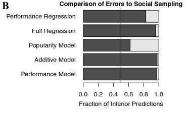
Figure S1: The horizontal bar plot indicates the relative error of each alternative model as compared to the social sampling model. Relative error is measured as the fraction of the alternative models’ prediction residuals that are larger than those of the social sampling model.

Finally, to better understand the relationship between these quantitative model comparison results and the qualitative results from Figure 2 in the main text, we further explored the distribution of model prediction errors for the three best models: social sampling, the popularity model, and the additive model. In this case we look at in-sample error after training on the entire dataset, which produces similar results to the cross-validation methods since the amount of data we have is so large compared to the number of parameters of each model. We examined the error of each model on the ten subsets of data defined by the data binning scheme used to generate the plots in Figure 2 of the main text. We find that for many subsets of the data (generally for users with positive performance, and for users with 10 mimickers or fewer), the predictions of these three models tend to be quite similar, and these three models achieve MSE and MAE within about 5% or less of each other on each of these subsets. However, for users with more than 100 mimickers and non-positive performance, social sampling achieves about 35% better MSE and MAE. Similarly, for users with between 10 and 100 mimickers and non-positive performance, social sampling achieves about 35% better MAE and about 10% better MSE. Since the dataset is unbalanced, the large gains in predictive performance that the social sampling model has on these subsets of the data are likely washed out by the many data points with low popularity or high popularity and high performance. This interpretation is consistent with the patterns evident in Figure 2 of the main text.

Table S3: Results using mean absolute error. Lower mean absolute error values are better.

Model	By User	By Day	In Future
Social Sampling	0.0391	0.0455	0.0403
Performance Model	0.0782	0.0783	0.0626
Additive Model	0.0402	0.0478	0.0420
Popularity Model	0.0400	0.0465	0.0409
Full Regression	0.0527	0.0569	0.0480
Performance Regression	0.0782	0.0783	0.0625

Table S4: Results using mean squared error. Lower mean squared error values are better.

Model	By User	By Day	In Future
Social Sampling	1.2924	2.1673	2.2389
Performance Model	3.0727	3.0683	2.3864
Additive Model	1.3194	2.1294	2.0707
Popularity Model	1.3215	2.1768	2.1428
Full Regression	2.1291	2.6120	2.0933
Performance Regression	3.0728	3.0682	2.3858

Table S5: Results using F-score. Higher F-score values are better.

Model	By User	By Day	In Future
Social Sampling	0.3978	0.4061	0.3619
Performance Model	0.0073	0.0000	0.0000
Additive Model	0.3874	0.3944	0.3418
Popularity Model	0.3873	0.3941	0.3446
Full Regression	0.3751	0.3775	0.3537
Performance Regression	0.0123	0.0007	0.0000

Robustness Checks

Finally, to further test the robustness of all our results to our choices in data parsing, we run the same set of analyses described in the previous sections using several alternative parses of our data. We test robustness to (a) the size of the rolling window used in our expected ROI computations, (b) the type of performance metric we use, (c) whether we use our imputed data or not, (d) whether we include only closed trades in our performance computation, and (e) which columns in our data we rely on for determining amounts invested and profit. We also check the results in our held-out year of data.

To test robustness to the performance metric used, we consider several alternatives. With our main ROI performance metric we check three alternative rolling window sizes of 1 day, 60 days, and 90 days. We also use two risk-adjusted performance metrics based on the Sharpe and Sortino ratios. The Sharpe metric is simply the expected ROI from closed trades divided by the standard deviation in those returns. The Sortino metric is the expected ROI divided by the standard deviation in the negative returns. Additionally, we consider the sum of profit from all trades (the “sum metric”), the sum of the profit from all trades divided by the total amount invested in all trades (the “average metric”), and the percentage of trades with positive profit minus 0.5 (the “percent metric”). For all these alternative metrics we use 30-day rolling windows.

For the other robustness checks, we maintain our usual 30-day ROI metric. To check robustness to whether we impute trades, we check the results without using imputed trades. To test robustness to whether we only use closed trades, we compute average ROI after simulating a liquidation of all open trades at the end of each day (in the same way as described in the section “Data Processing” above). To test robustness to which columns of our data we rely on, we recompute the profit from each trade and the amount invested in each trade via the total units purchased in those trades. We also use one additional ROI performance metric using the profit according to the units divided directly by the units invested to account for leverage.

Here we focus on an aggregate analysis of the results from these alternative data parses. We highlight the places where we have identified deviations from the results of our main analyses. In 12 out of 13 of these alternative parses we observe a statistically significant positive multiplicative interaction between previous popularity and previous performance in relation to changes in popularity using the ordinary linear model. The one exception is the parse using the Sortino metric.

The model comparison results are also highly robust, though slightly more mixed. In one case out of 39 total cases (counting the user, day, and future cross-validation approaches separately for each of the 13 different parses), the social sampling model has inferior mean absolute error. In four of the 12 alternative parses (the parses using rolling window 60, no data imputation, liquidating open trades, and the average metric), social sampling is inferior on mean squared error in the single method of cross validation that it was superior on in our main analysis. In two out of the 39 cases, social sampling has worse F-score (holding out the latest 10% using rolling window of 7 and using the percent metric). The relative error results are qualitatively similar to our main results for all models and all parses except that the popularity model achieves superior relative error in three out of the thirteen cases (rolling window 1, rolling window 7, and the percent metric).

The tests of the specific parameter fits of the social sampling model were also quite robust across many alternative parses. In every alternative parse, a scaling factor of 1.0 is the best fit exponential scaling factor on popularity, indicating strong evidence that popularity is used linearly rather than sublinearly or superlinearly. In every alternative parse at least one of the top ten traders’ confidence interval’s contains the best skill parameter according to the model. In four cases (percent metric, and rolling windows 1, 60, and 90), only three of the confidence intervals for the top 10 traders’ skills include the inferred best skill value. In one case (Sortino metric) six do. In the other eight alternative parses, between 7 and 10 do.

The results on our held-out validation set were similar to the aggregate results from the alternative parses, though somewhat weaker. As described in Section “Data Processing” above, we reserved one year of data as a nearly completely held-out validation set. This year ranged from July 1, 2012 until June 30, 2013. On this held out validation set, we used the 30-day ROI performance metric as in our main analysis. First, we again found evidence for the positive multiplicative interaction effect using the ordinary linear model. Next, the model comparison results were similar to those in our main analysis but somewhat weaker. The social sampling model again dominated in terms of mean absolute error, but lost in one out of three cases of the F-score and lost in all cases in mean squared error. Further, the relative error results were also similar to but somewhat weaker than the results in our main analysis. Once again social sampling achieves better error on more that 90% of cases compared with every model except the popularity model. The popularity model actually achieves better error on about 68% of the predictions, therefore beating social sampling under this relative error metric on the held out set. When performing a more fine-grained analysis of the errors, as we did with our model comparison results from the first year of data, we find once again that the predictions of the social sampling model, the popularity model, and the additive model are similar for many subsets of the data. However, the social sampling model predicts reliably better on low performance traders and substantially better on high popularity, low performance traders. Preferential attachment and the additive model do have noticeably better predictions on the single subset of traders with very high popularity and high performance, but still these gains are small compared to those of social sampling on the subsets where social sampling predicts well. As such, while the model comparison results on the held out set are slightly weaker, once again it appears that the highly unbalanced data makes the average errors overall look much different from the average errors within these relevant subsets of the data. The tests of the specific fit of the parameters of the social sampling model were highly robust in the held out set. Once again, the best fit scaling exponent on popularity was a linear fit. All ten of the top ten traders’ confidence interval’s included the inferred best skill value according to the model. Overall, our results are highly robust across alternative parses of the data, and moderately robust on the held-out data.

Possible Confounding Factors

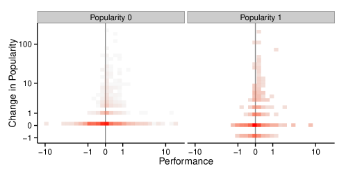
Figure S2: Evidence for a multiplicative interaction between popularity and performance in relation to changes in popularity even at low levels of popularity. The left panel includes all users on all days they have 0 mimickers, while the right panel includes all users on all days they had exactly 1 mimicker. The plots themselves are two-dimensional histograms (binned scatter plots). Higher red-value and lower transparency indicate higher density. The plot shows that users with one mimicker are expected to have greater increases in popularity than users with zero mimickers, and that this difference is mainly present in individuals with non-negative performance. As in the main text, the performance metric here is a 30-day rolling average of daily ROI, and change in popularity is the change in popularity on the following day. Running the regressions from the “Data Analysis” section above on the subset of data consisting of users with exactly zero or one mimicker yields a significant positive interaction term ($p<0.05$) with either ordinary or robust standard errors.

Our statistical analysis and model comparison allowed us to provide evidence that our results are likely not due to our apparent observed effects holding for just a few users, or on just a few days. Another possible limitation of our analysis is that we attempt to infer a causal mechanism from observational data. It is clear that changes in popularity cannot be causing previous popularity or previous performance, so a non-causal interpretation of our results would have to involve an unobserved variable. Such an unobserved variable would have to be correlated with both popularity and performance to cause the multiplicative interaction we observe. Among the possible alternative explanations of our results, the most likely is position bias. The issue of confounding position bias with social influence has been problematic for many previous related studies. A position bias occurs when a decision-maker is presented with a list of options. Those items at the top of the list tend to receive more attention and be selected more often simply because they are at the top of the list, not because they are any better in terms of underlying quality [37]. Thus, if the list is ordered by current popularity, a position bias can make it appear that highly popular items are being chosen more often.

There are two reasons that a position bias is unlikely to be responsible for our results. First and foremost, while it is possible for a position bias to account for a marginal effect of previous popularity on future popularity, position bias resulting from a single ordered list would not cause the multiplicative interaction we observe. Users would have to either have sorted by performance and popularity simultaneously for the position bias to cause that interaction, or some other feature of the interface would have to highlight users who were both popular and high performing. To the best of our knowledge, there was no straightforward way to sort by these two features simultaneously in the eToro interface at the time our data was collected. Furthermore, as shown in Figure S2, we observe the interaction between popularity and performance even at very low levels of popularity. While some users undoubtedly persistently scroll through the list of most popular traders down to those who have just one mimicker, a likely more common occurrence that could explain this interaction is that users sort according to a performance metric then prefer to consider mimicking users that have one mimicker as opposed to zero.

Anecdotal Evidence

One final piece of evidence supporting the social sampling model is a set of self-reports of actual users of eToro. Several users have posted advice online about how to effectively find traders to mimic on eToro. Two personal accounts we examined in detail broadly match the model we propose. The online advice points to sorting traders by popularity as the most reliable way to find potential traders to mimic, and the advice emphasizes that you should look carefully at a trader’s profile before deciding to mimic that trader to better judge the trader’s performance, even if the trader is highly popular. Both accounts also note that it’s not just the top most mimicked traders who are potentially good to mimic but that it is also productive to look for less popular options.

References

- [1] Iain D Couzin. Collective cognition in animal groups. Trends in Cognitive Sciences, 13(1):36–43, 2009.
- [2] Anita Williams Woolley, Christopher F Chabris, Alex Pentland, Nada Hashmi, and Thomas W Malone. Evidence for a collective intelligence factor in the performance of human groups. Science, 330(6004):686–688, 2010.
- [3] James Surowiecki. The Wisdom of Crowds. Anchor, 2005.
- [4] Edwin Hutchins. Cognition in the Wild. MIT Press, 1995.
- [5] Michael Kearns, Siddharth Suri, and Nick Montfort. An experimental study of the coloring problem on human subject networks. Science, 313(5788):824–827, 2006.
- [6] Iain D Couzin. Collective minds. Nature, 445(7129):715–715, 2007.
- [7] Ofer Feinerman and Amos Korman. Theoretical distributed computing meets biology: A review. In Distributed Computing and Internet Technology, pages 1–18. Springer, 2013.
- [8] Jessica R Mesmer-Magnus and Leslie A DeChurch. Information sharing and team performance: a meta-analysis. Journal of Applied Psychology, 94(2):535, 2009.
- [9] Ciro Cattuto, Alain Barrat, Andrea Baldassarri, Gregory Schehr, and Vittorio Loreto. Collective dynamics of social annotation. Proceedings of the National Academy of Sciences, 106(26):10511–10515, 2009.
- [10] Georg Theiner, Colin Allen, and Robert L Goldstone. Recognizing group cognition. Cognitive Systems Research, 11(4):378–395, 2010.
- [11] Luke Rendell, Robert Boyd, Daniel Cownden, Marquist Enquist, Kimmo Eriksson, Marc W Feldman, Laurel Fogarty, Stefano Ghirlanda, Timothy Lillicrap, and Kevin N Laland. Why copy others? Insights from the social learning strategies tournament. Science, 328(5975):208–213, 2010.
- [12] Winter Mason and Duncan J Watts. Collaborative learning in networks. Proceedings of the National Academy of Sciences, 109(3):764–769, 2012.
- [13] Andrey Rzhetsky, Jacob G Foster, Ian T Foster, and James A Evans. Choosing experiments to accelerate collective discovery. Proceedings of the National Academy of Sciences, 112(47):14569–14574, 2015.
- [14] Thomas L Griffiths and Joshua B Tenenbaum. Optimal predictions in everyday cognition. Psychological Science, 17(9):767–773, 2006.
- [15] Thomas L Griffiths, Charles Kemp, and Joshua B Tenenbaum. Bayesian models of cognition. In The Cambridge Handbook of Computational Psychology. Cambridge University Press, 2008.
- [16] Ginestra Bianconi and Albert-László Barabási. Bose-Einstein condensation in complex networks. Physical Review Letters, 86(24):5632, 2001.
- [17] Coco Krumme, Manuel Cebrian, Galen Pickard, and Alex Pentland. Quantifying social influence in an online cultural market. PLoS ONE, 7(5):e33785, 2012.
- [18] Alex Pentland. Social Physics: How Good Ideas Spread-The Lessons from a New Science. Penguin, 2014.
- [19] David JT Sumpter and Stephen C Pratt. Quorum responses and consensus decision making. Philosophical Transactions of the Royal Society B: Biological Sciences, 364(1518):743–753, 2009.
- [20] Richard McElreath, Adrian V Bell, Charles Efferson, Mark Lubell, Peter J Richerson, and Timothy Waring. Beyond existence and aiming outside the laboratory: Estimating frequency-dependent and pay-off-biased social learning strategies. Philosophical Transactions of the Royal Society B: Biological Sciences, 363(1509):3515–3528, 2008.
- [21] Bret Alexander Beheim, Calvin Thigpen, and Richard McElreath. Strategic social learning and the population dynamics of human behavior: The game of Go. Evolution and Human Behavior, 35(5):351–357, 2014.
- [22] Boris Granovskiy, Jason M Gold, David JT Sumpter, and Robert L Goldstone. Integration of social information by human groups. Topics in Cognitive Science, 7(3):469–493, 2015.
- [23] Stephen C Pratt, David JT Sumpter, Eamonn B Mallon, and Nigel R Franks. An agent-based model of collective nest choice by the ant Temnothorax albipennis. Animal Behaviour, 70(5):1023–1036, 2005.
- [24] Thomas D Seeley and Susannah C Buhrman. Group decision making in swarms of honey bees. Behavioral Ecology and Sociobiology, 45(1):19–31, 1999.
- [25] Tom Snijders. Stochastic actor-oriented models for network change. Journal of Mathematical Sociology, 21(1-2):149–172, 1996.
- [26] Morris H DeGroot. Reaching a consensus. Journal of the American Statistical Association, 69(345):118–121, 1974.
- [27] Sushil Bikhchandani, David Hirshleifer, and Ivo Welch. A theory of fads, fashion, custom, and cultural change as informational cascades. Journal of Political Economy, 100(5):992–1026, 1992.
- [28] Benjamin Golub and Matthew O Jackson. Naive learning in social networks and the wisdom of crowds. American Economic Journal: Microeconomics, pages 112–149, 2010.
- [29] Claudio Castellano, Santo Fortunato, and Vittorio Loreto. Statistical physics of social dynamics. Reviews of Modern Physics, 81(2):591, 2009.
- [30] Mark Granovetter. Threshold models of collective behavior. American Journal of Sociology, pages 1420–1443, 1978.
- [31] Edward Vul, Noah Goodman, Thomas L Griffiths, and Joshua B Tenenbaum. One and done? Optimal decisions from very few samples. Cognitive Science, 38(4):599–637, 2014.
- [32] Samuel J Gershman, Eric J Horvitz, and Joshua B Tenenbaum. Computational rationality: A converging paradigm for intelligence in brains, minds, and machines. Science, 349(6245):273–278, 2015.
- [33] Wei Pan, Yaniv Altshuler, and Alex Pentland. Decoding social influence and the wisdom of the crowd in financial trading network. In International Conference on Social Computing, pages 203–209, 2012.
- [34] Manuel Arellano. Computing robust standard errors for within-groups estimators. Oxford Bulletin of Economics and Statistics, 49(4):431–434, 1987.
- [35] Emilie Kaufmann, Nathaniel Korda, and Rémi Munos. Thompson sampling: An asymptotically optimal finite-time analysis. In Algorithmic Learning Theory, pages 199–213. Springer, 2012.
- [36] Sara Arganda, Alfonso Pérez-Escudero, and Gonzalo G. de Polavieja. A common rule for decision making in animal collectives across species. Proceedings of the National Academy of Sciences, 109(50):20508–20513, 2012.
- [37] Nathan O. Hodas and Kristina Lerman. The Simple Rules of Social Contagion. Scientific Reports, 4, 2014.