H₂S in the L1157-B1 Bow Shock

Abstract

Sulfur-bearing molecules are highly reactive in the gas phase of the ISM. However, the form in which most of the sulfur is locked onto interstellar dust grains is unknown. By taking advantage of the short time-scales of shocks in young molecular outflows, one could track back the main form of sulfur in the ices. In this paper, six transitions of H₂S and its isotopologues in the L1157-B1 bowshock have been detected using data from the Herschel-CHESS survey and the IRAM-30m ASAI large program. These detections are used to calculate the properties of H₂S gas in L1157-B1 through use of a rotation diagram and to explore the possible carriers of sulfur on the grains. The isotopologue detections allow the first calculation of the H₂S deuteration fraction in an outflow from a low mass protostar. The fractional abundance of H₂S in the region is found to be 6.0$\times$10^-7 and the deuteration fraction is 2$\times$10^-2. In order to investigate the form of sulfur on the grains, a chemical model is run with four different networks, each with different branching ratios for the freeze out of sulfur bearing species into molecules such as OCS and H₂S. It is found that the model best fits the data when at least half of each sulfur bearing species hydrogenates when freezing. We therefore conclude that a significant fraction of sulfur in L1157-B1 is likely to be locked in H₂S on the grains.

1 Introduction

Low mass protostars drive fast jets during the earliest stages of their evolution. The collision between these jets and the protostar’s parent cloud is supersonic, producing shock fronts of warm, dense gas. This in turn drives processes that greatly increase the chemical complexity, such as endothermic reactions, sputtering from dust grains and ice mantle sublimation. Many molecular species are enhanced in abundance through this process (Draine et al., 1983; van Dishoeck & Blake, 1998; Codella et al., 2013) and the observation and modelling of these species is a powerful tool for understanding their gas-phase chemistry and the initial preshock composition of the ices on the grains.

L1157-mm is a Class 0, low mass protostar driving a molecular outflow (Gueth et al., 1997) and is at a distance of 250 pc (Looney et al., 2007). The outflow was discovered by Umemoto et al. (1992) who also inferred the presence of strong shocks from the temperature of the gas implied by NH₃ and SiO emission. Since then, several bow shocks along the outflow have been identified and studied due to their rich chemical content. The brightest of these, L1157-B1, has a complex, clumpy structure (Tafalla & Bachiller, 1995; Benedettini et al., 2007) and an age of order 1000 yr constrained by observations (Gueth et al., 1998) and models (Flower & Pineau des Forêts, 2012). Emission from molecules thought to be formed on icy mantles such as methanol and water have been observed (Bachiller & Pérez Gutiérrez, 1997; Busquet et al., 2014). This high degree of study of the L1157 outflow has led to it being considered the prototype of a chemically rich molecular outflow (Bachiller et al., 2001). Therefore, L1157 represents the best laboratory to study the initial composition of the ices.

Through the IRAM large program ASAI (Astrochemical Surveys At IRAM) and the Herschel Key project CHESS (Chemical HErschel Surveys of Star forming regions), a spectral survey of L1157-B1 has been performed in the frequency ranges of 80-350 GHz (IRAM-30m/EMIR) and 500-2000 GHz (Herschel-HIFI). The first results of the CHESS survey (Codella et al., 2010; Lefloch et al., 2010) confirmed the chemical richness of the bow shock. Constraints on the gas properties were found using CO. Lefloch et al. (2012) found the line profiles could be fitted by three velocity components of the form $I(v)\propto exp(-|v/v_{0}|)$, tracing three kinematic components of the gas (see Sect. 3.2). Gómez-Ruiz et al. (2015) found two of these components could fit the CS emission from L1157-B1. An LVG analysis of water emission detected by Herschel-HIFI indicated one of these components could explain most of the water emission though the higher E_u transitions required a hot component that had not been identified in previous studies (Busquet et al., 2014). This implies that these velocity components likely represent distinct physical conditions in the gas. Several studies have started to compare the observed species with chemical models to derive the properties of the shock in L1157-B1 (Viti et al., 2011; Benedettini et al., 2012, 2013). Podio et al. (2014) reported the emission of molecular ions, including SO⁺ and HCS⁺, whose chemistry is closely related to the amount of S-bearing molecules released from dust grains, such as H₂S and OCS.

Sulfur is highly reactive and therefore its chemistry is very sensitive to the thermal and kinetic properties of the gas. That chemistry, if it were well understood, could be used to constrain the properties of the bow shock or regions within it. In fact, H₂S has been studied along with SO and SO₂ as a chemical clock for environments where dust grains are disrupted since it was first proposed by Charnley (1997). A key assumption for this is that H₂S is one of the most abundant sulfur bearing species on ice mantles (Wakelam et al., 2004) and is then released into the gas phase during a shock. This assumption requires further study to determine its veracity. OCS and SO₂ are the only sulfur-bearing species firmly detected in the solid phase so far (Geballe et al., 1985; Palumbo et al., 1995; Boogert et al., 1997). In fact, the chemical model presented in Podio et al. (2014) in order to reproduce the abundance of CS and HCS⁺ observed in L1157-B1 indicated that OCS could be one of the main sulfur carriers on dust grains. Despite this, detections of solid OCS give abundances that would account for only $\sim$0.5% of the cosmic sulfur abundance (Palumbo et al., 1997). Since estimates of grain-surface OCS abundances may be affected by blending with a nearby methanol feature in infra-red spectra, it is possible that much sulfur is eventually locked in solid OCS.

Other forms of sulfur have been considered. Woods et al. (2015) investigated the gas and solid-phase network of sulfur-bearing species using new experimental and theoretical studies (Garozzo et al., 2010; Ward et al., 2012; Loison et al., 2012). They found that although species such as H₂S and H₂S₂ are present on the ices, they are not sufficiently abundant to be the major carriers of sulfur. In fact, a residue of atomic sulfur may be abundant enough to harbor a large amount of the total sulfur budget. This residue may come off during sputtering if a fast enough shock is present. A shock velocity of 25 km s^-1 is likely to be sufficient to release even highly refactory species from the grains (May et al., 2000). One would expect to commonly observe chemistry involving atomic sulfur in shocked regions as this sulfur residue is sputtered from the mantle at such shock velocities. They also found that H₂S is in fact the predominant sulfur-bearing species at the early phases of the pre-stellar core.

In summary, H₂S is routinely observed in warm, sometimes shocked environments, in the gas phase; yet it is undetected in the ices to date. Given the uncertainty of the origin of H₂S on grains and the fact that L1157-B1 contains gas that is highly processed by shocks, the physical properties and kinematics of the H₂S gas could help determine its chemical origin.

In this paper we present H₂S observations along the L1157-B1 clump and by the use of a gas-grain chemical and parametric shock model we attempt to discover its origin and its relationship to other sulfur-bearing species. In Sect. 2, the observations with HIFI and the IRAM 30m telescope are described. In Sect. 3, the detected H₂S lines are presented and analyzed. In Sect. 4, the abundance and behaviour of H₂S is compared to CS and NH₃ as well as to a chemical model in which the form of sulfur in ice mantles is explored. Finally, the paper is summarized in Sect. 5.

2 Observations

2.1 IRAM-30m

Figure 1: CO (1-0) map of the L1157 region (Gueth et al., 1996), including the protostar L1157-mm and the southern outflow. The dashed and solid rings show the beamsizes of IRAM-30m/EMIR and Herschel/HIFI respectively for the transitions detected. The triangle within the rings marks the position of the B1 shock and the other triangle marks the position of the protostar L1157-mm.

The H₂S and H${}_{2}^{34}$S (1_1,0-1_0,1) lines as well as the HDS (1_1,0-0_0,0) were detected during the ASAI program’s unbiased spectral survey of L1157-B1 with the IRAM 30m telescope. The pointed co-ordinates were $\alpha_{J2000}=20^{h}39^{m}10.2^{s}$, $\delta_{J2000}=+68^{\degree}01^{\prime}10".5$ i.e. $\Delta\alpha=+25".6$, $\Delta\delta=-63".5$ from the driving protostar. NGC7538 was used for pointing, which was monitored regularly. It was found very stable with corrections less than 3". The observed region and the relevant beamsizes for the observations presented here are shown in Fig. 1. The broadband EMIR receivers were used with the Fourier Transform Spectrometer backend which provides a spectral resolution of 200 kHz, equivalent to 0.35 km s^-1 for the transitions at around 168 GHz. The transition at 244 GHz was smoothed to a velocity resolution of 1.00 km s^-1 to improve the signal to noise ratio. Forward and beam efficiencies are provided for certain frequencies (Kramer et al., 2013) and a linear fit gives a good estimate when interpolating between points. Table 2 gives these efficiencies as well as the telescope half power beamwidth at the observed frequencies. Line intensities were converted to units of T_MB by using the B_eff and F_eff values given in Table 2.

2.2 Herschel-HIFI

The H₂S (2_0,2-1_1,1), (2_1,2-1_0,1) and HDS (2_1,2-1_0,1) transitions were detected with Herschel (Pilbratt et al., 2010) using the HIFI instrument (de Graauw et al., 2010), in bands 2A, 2B and 1B respectively as part of the CHESS spectral survey. The observations were done in double beam switching mode, with the pointed co-ordinates being the same as the IRAM-30m observations. The receiver was tuned in double sideband and the Wide Band Spectrometer was used. At the frequencies observed, the pointing of the H and V polarisations can differ by as much as 5". However, the spectra are in good agreement having similar rms values, line profiles and fluxes for detected lines and are therefore averaged. The data were processed using ESA supported package HIPE 6 (Herschel Interactive Processing environment, Ott 2010) and fits files from level 2 were exported for further reduction in GILDAS. The resulting spectra have a velocity resolution of 0.25 km s^-1 and an rms of 3.6 mK. Values for beam efficiency were taken from Roelfsema et al. (2012) and adjusted for wavelength by a Ruze formula given in the same article.

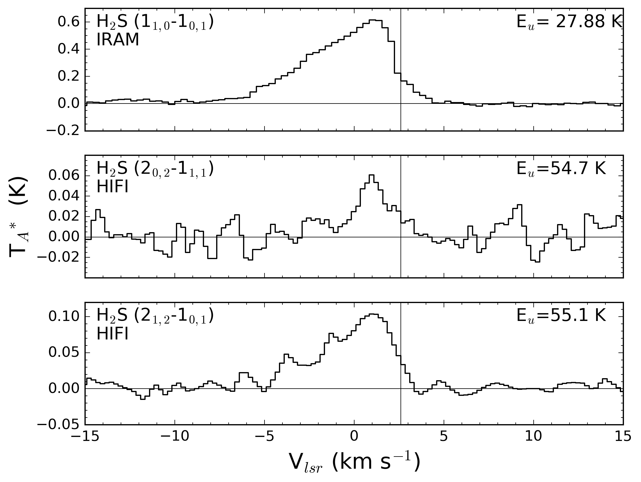
Figure 2: Herschel/HIFI and IRAM-30m/EMIR detections of the H₂S main isotopologue. The vertical line indicates the cloud velocity V${}_{sys}=$2.6 km s^-1.

Figure 3: Herschel/HIFI and IRAM-30m/EMIR detections of H₂S isotopologues. The HDS lines are at lower spectral resolution than the other detections. The HDS (1-0) spectrum has a resolution of 1 km s^-1 and HDS (2-1) spectrum has a resolution of 0.5 km s^-1.

Table 1: Details of Herschel/HIFI observations.

Frequency	Band	Obs_Id	Date
(GHz)
687.3	2a	1342207607	2010-10-28
736.0	2b	1342207611	2010-10-28
582.4	1b	1342181160	2009-08-01

Table 2: List of detected lines and the relevant spectroscopic and instrument properties. Ortho and para species are denoted by o- and p- respectively. All spectroscopic data were taken from Pickett et al. (1998).

Molecule	Transition	Freq	Eu	gu	log(Aul)	Instrument	Tsys	$\theta_{beam}$	$\Delta$V	Beff	Feff
		(GHz)	(K)				(K)	(")	(km s-1)
o-H2S	11,0-10,1	168.7628	27.9	9	-4.57	IRAM-30m/EMIR	132	15	0.35	0.74	0.93
p-H2S	20,2-11,1	687.3035	54.7	5	-3.03	Herschel/HIFI	137	31	0.25	0.76	0.96
o-H2S	21,2-10,1	736.0341	55.1	15	-2.88	Herschel/HIFI	317	29	0.25	0.77	0.96
o-H${}_{2}^{34}$S	11,0-10,1	167.9105	27.8	9	-4.58	IRAM-30m/EMIR	159	15	0.36	0.74	0.93
o-HDS	10,1-00,0	244.5556	11.7	3	-4.90	IRAM-30m/EMIR	190	10	1.00	0.59	0.92
o-HDS	21,2-10,1	582.3664	39.7	5	-3.18	Herschel/HIFI	84	36	0.50	0.77	0.96

Table 3: Derived parameters of the detected lines. T_peak is given in units of T_mb and Vmin/Vmax are where lines drop below 3$\sigma$ levels except for HDS lines where 1$\sigma$ is used (See Sect. 3.1). Parenthesized values are uncertainties.

Molecule	Transition	Tpeak	Vpeak	Vmin/Vmax	$\int$ Tmb dv
		(mK)	(km s-1)	(km s-1)	(K km s-1)
o-H2S	11,0-10,1	614 (8)	1.05	-7.90/4.70	4.41 (0.90)
p-H2S	20,2-11,1	60 (9)	1.00	0.10/2.10	0.20 (0.03)
o-H2S	21,2-10,1	103 (9)	1.25	-4.15/3.10	0.58 (0.07)
o-H${}_{2}^{34}$S	11,0-10,1	46 (6)	0.65	-1.69/2.96	0.28 (0.06)
o-HDS	10,1-00,0	8 (2)	1.00	0.60/3.60	0.030 (0.008)
o-HDS	21,2-10,1	19 (6)	0.00	0.00/2.50	0.034 (0.009)

3 Results

3.1 Detected Lines and Opacities

In total, six lines were detected including H${}_{2}^{34}$S and HDS as well as the main isotopologue, H₂S. Table 2 gives the telescope and spectroscopic parameters relevant to each detected line. Frequencies ($\nu$), quantum numbers, Einstein coefficients (A_ul), and the upper state energies (E_u) and degeneracies (g_u) are taken from the JPL spectral line catalog (Pickett et al., 1998). The measured line properties including the velocities V_min and V_max taken to be the velocities at which the emission falls below the 3$\sigma$ level, and the integrated emission ($\int T_{MB}dv$) within those limits are shown in Table 3. The error quoted for the integrated intensities includes the propagated error from the rms of T_MB and the velocity resolution of the spectra as well as nominal calibration errors of 10 and 20% for Herschel-HIFI and IRAM-30m respectively. Note that the HDS spectra are at lower spectral resolution and have less significant detections than the other H₂S transitions, each peaking between the 3 and 4 $\sigma$ level. For this reason, the velocity limits of the HDS (2-1) transition are taken to be where the peak is above 1$\sigma$.

Figures 2 and 3 show the six lines labelled by their species and quantum numbers. The spectra are given in units of antenna temperature T${}_{a}^{*}$. Figure 2 shows the three H₂S lines whilst Fig. 3 shows the isotopologues. In Fig. 2, the H₂S (2_1,2-1_0,1) line shows three peaks. The primary peak is at 1.25 km s^-1, which is common to all the spectra. The secondary peak at -3.75 km s^-1 is consistent with lines detected in L1157-B1 by Codella et al. (2010) who found that HCN, NH₃, H₂CO and CH₃OH showed primary peaks at approximately 1 km s^-1 and secondary peaks between -3 and -4 km s^-1. However, the peak at -1.25 km s^-1 in the H₂S (2_1,2-1_0,1) spectrum is not consistent with any other spectral features and may be due to a contaminant species or simply noise.

The 1_1,0-1_0,1 transition has been detected in both H₂S and H${}_{2}^{34}$S, allowing the optical depth of L1157-B1 for H₂S to be calculated. Equation 1 gives the source averaged column density of the upper state of a transition, $N_{u}$, when the source is much smaller than the beam and optical depth, $\tau$ is non-negligible. $ff$ is a correction for the fact the emission does not fill the beam.

$$N_{u}=\frac{8\pi k\nu^{2}}{hc^{3}A_{ul}}ff\int T_{MB}dv\left(\frac{\tau}{1-e^{-\tau}}\right)$$ (1)

It is assumed that all the H₂S emission comes from B1. Whilst previous work on L1157-B1 has suggested most emission comes from the walls of the B1 cavity (Benedettini et al., 2013), this has not been assumed and the entire size of B1 is used. Thus, size was taken to be 18" in agreement with the size of B1 in CS estimated by Gómez-Ruiz et al. (2015) from PdBI maps by Benedettini et al. (2013). The validity of this assumption is explored in Sect. 3.2. However, it should be noted that varying the size from 15" to 25" changes ln($\frac{N_{u}}{g_{u}}$) by less than 1% and encompasses all estimates of the source size from other authors (Lefloch et al., 2012; Podio et al., 2014; Gómez-Ruiz et al., 2015).

For the equivalent transition in a pair of isotopologues, it is expected that $N_{u}$ would only differ by the isotope abundance ratio if the emission region is the same. A ³²S/³⁴S ratio, R, of 22.13 was assumed (Rosman & Taylor, 1998) and tested by comparing the integrated emission in the wings of the 1_1,0-1_0,1 transitions; that is all of the emission below -1 km s^-1. This emission is likely to be optically thin, allowing us to test the abundance ratio. A ratio of 22$\pm$3 was found, consistent with the value taken from the literature. Using Eq. 2 below with the measured integrated line intensities, an optical depth for H₂S (1_1,0-1_0,1) of $\tau=$0.87 was calculated. It is assumed that H${}_{2}^{34}$S is optically thin.

$$\frac{1-e^{-\tau}}{1-e^{-\tau/R}}=\frac{\int T_{MB}(^{32}S)dv}{\int T_{MB}(^{34}S)dv}$$ (2)

Figure 4: Log-linear plots of the well detected transitions. The dashed and dotted fits are $I(v)\propto exp(-|v/v_{0}|)$ profiles with v₀ = 4.4 km s^-1 (g₂) and 2.5 km s^-1 (g₃) respectively. The solid line is the best fit line, a linear combination of the other two. The third component, g₁ (v₀=12.5 km s^-1) is not shown as it is not required for the best fit and there is no emission from velocities more blue shifted than -8 km s^-1. The vertical line is the cloud velocity, V${}_{sys}=$2.6 km s^-1 (Bachiller & Pérez Gutiérrez, 1997), and the horizontal line marks each the 3$\sigma$ rms level on each plot.

3.2 Origin of the Emission

Lefloch et al. (2012) found that the CO emission from L1157-B1 could be fitted by a linear combination of three velocity profiles, associated with three physical components. The profiles were given by $I(v)\propto exp(-|v/v_{0}|)$ where $v_{0}$ is the characteristic velocity of the physical component. The velocities were 12.5 km s^-1, 4.4 km s^-1 and 2.5 km s^-1 which are respectively associated with a J shock where the protostellar jet impacts the B1 cavity, the walls of the B1 cavity and an older cavity (B2). These components were labelled as g₁, g₂ and g₃ and the same notation is used here for consistency. This has also been applied to other molecules. For CS (Gómez-Ruiz et al., 2015), it was found that the g₂ and g₃ components fit the CS lines well with a negligible contribution from the g₁ component except for the high J lines detected with HIFI. The same was found to be true for SO⁺ and HCS⁺ (Podio et al., 2014). This implies that the majority of emission from the low energy transitions of sulfur bearing molecules comes from the B1 and B2 cavities and is not associated with the J-shock.

The three components have been used to fit the H₂S line profiles and the results are shown in Fig. 4. The fit for H₂S (2_0,2-1_1,1) is not shown as the detection is not significant enough to be well fitted. Unlike other molecules in the region, the fits for H₂S appear to be fairly poor, with reduced $X^{2}$ values much greater than 1 for H₂S (1_1,0-1_0,1) and the H₂S (2_1,2-1_0,1) suffering from the secondary peaks. We also note that the H₂³⁴S isotopologue is well fitted. In each case, only the g₂ and g₃ components are required for the best fit. This implies that, as for CS, the majority of the H₂S emission arises from B1 and B2 cavities affected by the interaction of low-velocity C-shock. Since the g₁ component is negligible in the H₂S lines, the nearby J-shock does not contribute to their emission. This justifies the use of a C-shock model in Sect. 4.2 to reproduce the observed line profiles and measured abundances of H₂S in L1157-B1.

3.3 Column Densities and Abundances

The three detected transitions of H₂S allow the excitation temperature and column density of the shocked gas in L1157-B1 to be calculated through use of a rotation diagram (Goldsmith & Langer, 1999). Of the three transitions, one is para-H₂S and the other two are ortho. In order to proceed, an ortho-to-para ratio needs to be assumed. Given the lack of further data, the statistical average of 3 is assumed for the ortho-to-para ratio. Reducing this ratio to 1 produced results within error of those presented here for column density and temperature. It is therefore not possible to draw any conclusions about the ortho-to-para ratio from the data available.

The H₂S column density and temperature were calculated through the use of a rotation diagram. For the rotation diagram, the upper state column density, $N_{u}$ was calculated from Eq. 1 assuming all three transitions had the same optical depth, calculated above. The filling factor in Eq. 1, $ff$ is uncertain due to the fact that Sect. 3.2 shows that H₂S emission comes partially from the walls of the B1 cavity and partially from the older B2 cavity. For the calculations here, we adopt a source size of 18" but as noted in Sect. 3.1, a size of 25" gave the same result. The rotation diagram is shown in Fig. 5 and gave an excitation temperature of 13$\pm$6 K. This is consistent with the low temperature of the g₃ component calculated as $\sim$23 K by Lefloch et al. (2012). Using the JPL partition function values for H₂S (Pickett et al., 1998), a total column density was found to be $N(H_{2}S)$=6.0$\pm$4.0$\times$10¹⁴ cm^-2.

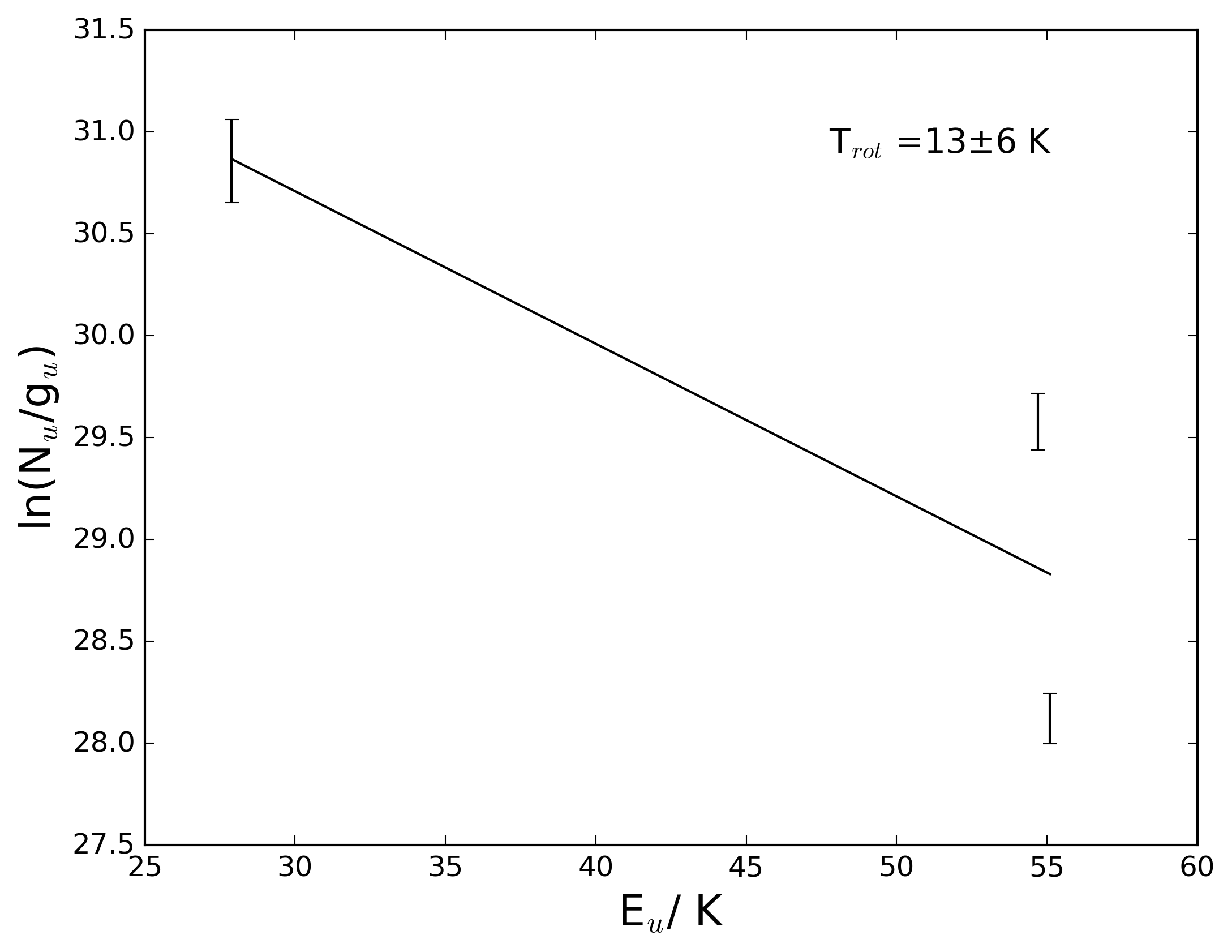
Figure 5: Rotation diagram for H₂S. The gradient gives an excitation temperature of 13 K and the intercept gives a column density of 6.0$\pm$4.0 $\times$10¹⁴ cm^-2 at that temperature.

Bachiller & Pérez Gutiérrez (1997) calculated a fractional abundance of H₂S by comparing measured column densities of H₂S to CO and assuming a CO:H₂ ratio of 10^-4. They obtained a value of 2.8$\times$10^-7. Given that their H₂S column density was calculated from a single line by assuming a temperature of 80 K and optically thin emission, an updated value has been calculated. For the CO column density, a more recent measurement of N(CO)=1.0$\times$10¹⁷ cm^-2 is used (Lefloch et al., 2012). For a H₂S column density of 6.0$\times$10¹⁴ cm^-2, a fractional abundance X= 6.0$\times$10^-7 is found. This is a factor of $\sim$2 larger than the Bachiller & Pérez Gutiérrez measurement, most likely due to the improved column density derived by using a rotation diagram with three transitions rather than a single line with an assumed temperature.

It should be noted that the critical densities for the two higher frequency transitions are n${}_{c}\sim 10^{7}cm^{-3}$. Estimates of the average number density in B1 and B2 are of order n${}_{H}\sim 10^{5}cm^{-3}$. Therefore LTE is unlikely to apply here. This casts doubt on the rotation diagram method and so the radiative transfer code RADEX (van der Tak et al., 2007) was run with a range of column densities, gas densities and temperatures to see if similar results would be obtained. H₂ number densities in the range $n=10^{4}-10^{6}cm^{-3}$ and temperatures in the range 10-70 K were used based on the values found for g₂ and g₃ with LVG modelling by Lefloch et al. (2012). With these parameters, the best fit found by comparing predicted brightness temperatures to the H₂S lines reported here is 3.0$\times 10^{14}cm^{-2}$ at a temperature of 10 K and density 10⁵cm^-3. Fits with T > 30 K or n_H $\gg$ 10⁵cm^-3 were always poor.

3.4 The Deuteration Fraction of H₂S

The excitation temperature is further used to make the first estimate of the deuteration fraction of H₂S in an outflow from a low mass protostar. The integrated intensities of the HDS emission lines are used to calculated $ln(N_{u})$ for each transition, again assuming a source of 18". We then use T_ex=13$\pm$6 K, the value of the partition function, Z, and upper state degeneracy g_u taken from the JPL catalog to find a column density for HDS as

$$ln(N)=ln(\frac{N_{u}}{g_{u}})+ln(Z)+\frac{E_{u}}{kT_{ex}}$$ (3)

By averaging the column density obtained from each of the two transitions, a column density of 2.4$\pm$1.2$\times$10¹³ cm^-2 is found. This corresponds to a deuteration fraction for H₂S of 2.5$\pm$2.5$\times$10^-2. As these abundances are an average over the beam, this is likely to be a lower limit of the true deuteration on the grains. However, it is comparable to level of deuteration measured for other species in L1157-B1. For example, the methanol deuteration fraction was found to be 2$\times$10^-2 by Codella et al. (2012). Further, Fontani et al. (2014) detected HDCO, CH₂DOH with the Plateau de Bure interferometer and compared to previous measurements of CH₃OH and H₂CO. They obtain higher deuteration fractions for H₂CO and CH₃OH than the H₂S value reported here. However, they note that the PdBI detections of the H₂CO and CH₃OH that they use may be resolving out as much as 60% of the emission, leading to higher deuteration fractions and so claim consistency with the Codella et al. (2012) results. Therefore, deuterated H₂S appears to be consistent with many deuterated molecules in L1157-B1.

4 Sulfur Chemistry in the B1 Shock

4.1 Comparison of Line Profiles

In the previous section we postulate that H₂S arises, like CS, from the B1 and B2 cavity. In order to test this hypothesis, we compar the emission of these species to see if they show similar behaviour. Figure 6 shows the ratios of the line temperatures for the H₂S (1_1,0-1_0,1) transition with the CS (3-2) and NH₃ (1-0) transitions. This allows us to better compare the line profiles and the evolution of the molecular abundances of the different species considered in this section and in Sect. 4.2. The spectra have been re-sampled to common velocity bins. The H₂S (1_1,0-1_0,1) transition was chosen as it is both less noisy than the other H₂S transitions and closer in excitation properties to the available CS and NH₃ transitions.

The CS transition in Fig. 6a is the CS (3-2) transition at 146.97 GHz; it has an upper level energy of E${}_{u}=$ 14.1 K. Figure 6a shows that the CS (3-2) and H₂S (1_1,0-1_0,1) profiles differ by a factor of $\sim$10 at higher velocities. Assuming that the line ratio follows the behaviour of the abundance ratio between these two species, this may imply that H₂S is not as abundant as CS at higher velocities and therefore raises the possibility that the H₂S and CS emission do not entirely arise from the same region. This pattern is attributed to chemical differences between the molecules and explored in Sect. 4.2.

The NH₃ spectrum in Fig. 6b is the NH₃ (1-0) line at 572.49 GHz, it has an upper level energy of E${}_{u}=$ 27.47 K which is comparable to the upper level energy of the H₂S (1_1,0-1_0,1) transition. These two transitions are compared due to their similar excitation properties and strong detections; the other H₂S spectra are much noisier. From Fig. 6b, we find that the H₂S and NH₃ intensities (and thus, their abundances) differ by less than a factor of 3 throughout the postshock gas, which suggests that H₂S and NH₃ come from the same region and behave similarly. We however note that the NH₃ line has been measured within a larger beam than H₂S and thus, the NH₃ line may include emission from a larger area in the L1157-B1 bowshock.

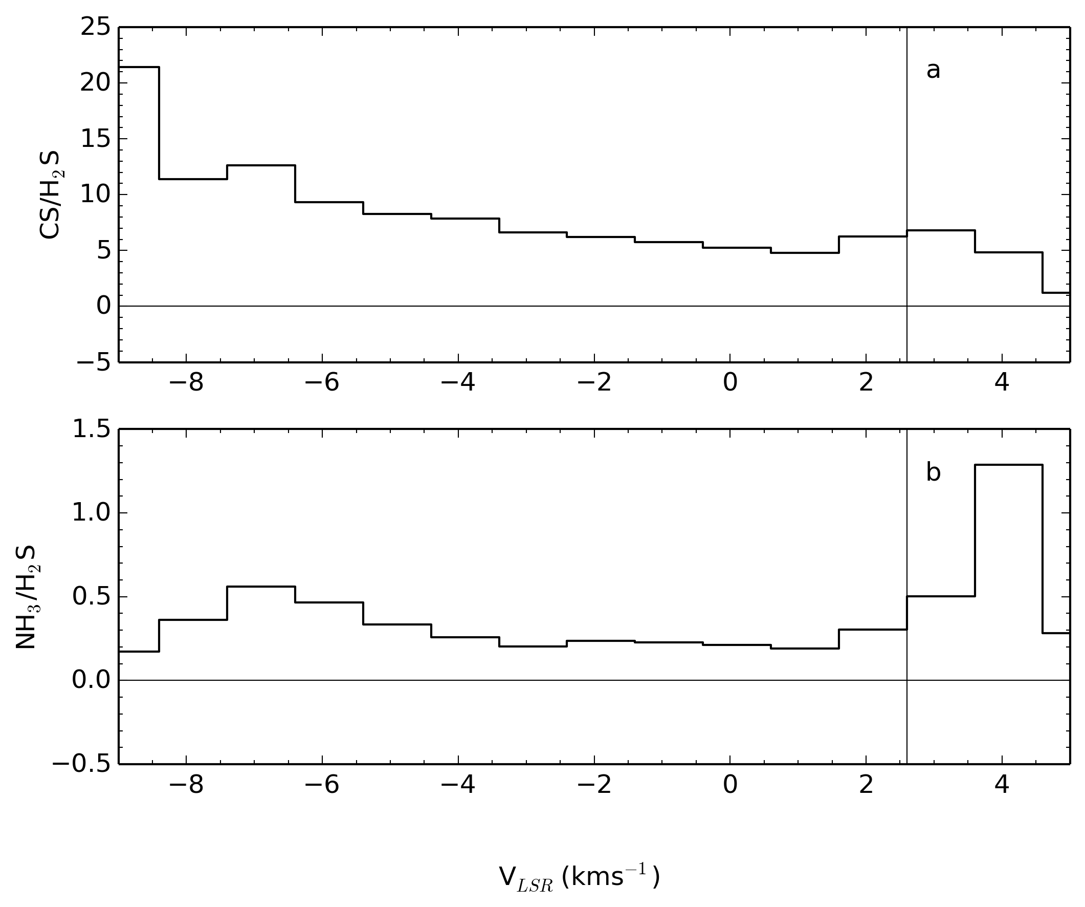
Figure 6: Emisson ratios CS (3-2)/H₂S (a) and NH₃ (1-0)/H₂S (b). The H₂S (1_1,0-1_0,1) line is used in both. All the spectra have been resampled into bins with a common resolution of 1 km s^-1 centred at 2.6km s^-1. The 3$\sigma$ velocity limits of the H₂S line are used to set the x-axis as they give the smallest velocity range in each case.

4.2 Comparison with Chemical Models

We have established that the H₂S spectra do not require a g₁ component to be well fitted and are therefore not likely to be associated with the J shock from L1157-mm’s outflow (see Sect. 3.2). Extensive efforts have been made to model the dynamics of L1157-B1 with C-shocks (e.g. Gusdorf et al., 2008; Flower & Pineau des Forêts, 2012) and have proven successful. The line profiles of H₂S appear to be consistent with the shapes predicted for other molecules from a parameterized C-shock model in Jiménez-Serra et al. (2009) and the behaviour of other species such as H₂O and NH₃ have been successfully modelled by coupling the same shock model with a chemical code (Viti et al., 2011). Hereafter we thus assume that the sulfur chemistry observed toward L1157-B1 can be modelled by a C-type shock. Through this modelling, we investigate whether H₂S is formed mainly on the grains or in the gas phase during the passage of a C-type shock. We shall use the same model as in Viti et al. (2011), ucl_chem, which is a gas-grain chemical model coupled with a parametric shock model (Jiménez-Serra et al., 2008). The model is time-dependent and follows the abundances of molecular species through two phases.

In phase I, the formation of a molecular cloud is modelled including gravitational collapse, freeze out onto dust grains and surface chemistry. This gives a self consistent rather than assumed ice mantle and gas phase abundances for phase II.

In phase II, the propagation of a C-type shock from the protostellar outflow is modelled according to the Jiménez-Serra et al. (2008) parameterization. The physical structure of the shock is parameterized as a function of the shock velocity (V_s), and the H₂ gas density of the preshock gas. The magnetic field used in the model is 450 $\mu$G, transverse to the shock velocity, and it has been calculated following the scaling relation B₀($\mu$G) = b₀ x $\sqrt{n_{0}(cm^{-3})}$ with b₀ = 1 following Draine et al. (1983) and Le Bourlot et al. (2002). Note that in this one case, the density n₀ is given as the density of hydrogen nuclei. The maximum temperature of the neutral fluid attained within the shock (T_n,max) is taken from Figures 8b and 9b in Draine et al. (1983). The sputtering of the grain mantles is simulated in the code by introducing a discontinuity in the gas-phase abundance of every molecular species once the dynamical time across the C-shock has reached the “saturation time-scales”. The “saturation times” were defined by Jiménez-Serra et al. (2008) as the time-scales at which the relative difference in the sputtered molecular abundances between two consecutive time steps in the model are less than 10%, and represent a measure of the time-scales for which almost all molecular material within the mantles is released into the gas phase. For the saturation times for H₂S and the other sulfur-bearing species, we adopt those already derived for SiO coming from the mantles (see Table 5 in Jiménez-Serra et al. (2008)). The mathematical expression for the sputtering of the grain mantles for any molecular species is the same except for the initial solid abundance in the ices (see Eqs. B4 and B5 in the same paper). Consequently, species differ in the absolute scale in the final abundance sputtered from grains but not the time-scales at which they are injected into the gas phase.

We have used the best fit model from Viti et al. (2011). In this model, the C-shock has a speed of v_s=40 km s^-1 and the neutral gas reaches a maximum temperature of T_n,max=4000 K in the postshock region. As shown by Le Bourlot et al. (2002) and Flower & Pineau des Forêts (2003), C-shocks can indeed develop in a medium with a pre-shock density of 10⁵ cm^-3 and magnetic induction B₀=450 $\mu$G (or b₀=1; see their Figures 1 and 5). Although the terminal velocity of the H₂S shocked gas observed in L1157-B1 is only about -10 km s^-1, the higher shock velocity of vs= 40 km s^-1 used in the model is justified by the fact that other molecules such as H₂O and CO show broader emission even at terminal velocities of -30 km s${}^{-}1$ and -40 km s^-1 (Codella et al., 2010; Lefloch et al., 2010). These are expected to be more reflective of the shock velocity as these molecules are not destroyed at the high temperatures produced by the shock and so remain abundant out to high velocities (Viti et al., 2011; Gómez-Ruiz et al., 2016).

We note that recent shock modelling assuming perpendicular geometry of the shock predicts thinner postshock regions, and consequently higher T_max in the shock, than those considered here under the same initial conditions of preshock gas densities and shock velocities (see e.g. Guillet et al., 2011; Anderl et al., 2013). However, MHD simulations of oblique shocks (van Loo et al., 2009) seem to agree with our lower estimates of T_n,max and therefore, we adopt the treatment proposed by Jiménez-Serra et al. (2008). The validation of this parameterization is discussed at length in Jiménez-Serra et al. (2008). The interested reader is referred to that paper for details of the C-shock modelling and to Viti et al. (2004) for details on ucl_chem.

In the model, we have expanded the sulfur network following Woods et al. (2015) to investigate the composition of the ice mantles. The first three versions of the network were taken directly from Woods et al. (2015). The behaviour of sulfur bearing species are as follows (see Table 5):

• A Species froze as themselves.

• B Species immediately hydrogenated.

• C Species would freeze 50% as themselves and 50% hydrogenated.

• D Any species for which a reaction existed to produce OCS on the grains was set to freeze out entirely as OCS.

• E Species would freeze 50% as themselves and 50% as OCS if possible.

The injection of the ice mantles into the gas phase by sputtering occurs once the dynamical time in the C-shock exceeds the saturation time, i.e. when t_dyn >4.6 years. No grain-grain interactions are taken into account due to the computational costs.

The parameter values for the C-shock in the model are given in Table 4. Note network D is not reflective of real chemistry but rather takes the extreme case of highly efficient grain surface reactions allowing frozen sulfur, carbon and oxygen atoms to form OCS.

Table 4: Model parameters.

n(H2)	105 cm-3
Vs	40 km s-1
tsat	4.6 yr
Tn,max	4000 K
B0	450 $\mu$G

Note: n($H_{2}$) is the pre-shock hydrogen density, V_s is the shock speed, t_sat is the saturation time, T_n,max is the maximum temperature reached by the neutral gas.

Table 5: Branching ratios for the freeze out routes of example sulfur bearing species in each model. Where a # indicates a frozen species.

Model	S	HS	CS
Model A	100% #S	100% #HS	100% #CS
Model B	100% #H2S	100% #H2S	100% #HCS
Model C	50% #S	50% #HS	50% #CS
	50% #H2S	50% #H2S	50%#HCS
Model D	100% #OCS	50% #HS	100% #OCS
		50% #H2S
Model E	50% #OCS	50% #HS	50% #OCS
	50% #H2S	50% #H2S	50% HCS

Figure 7 shows the results from four of the networks used to investigate the conditions of the shock in L1157-B1. In each case only phase II is shown, the initial abundances at log(Z)=14 are the final abundances of phase I from each network. As explained above, sputtering occurs once t_sat is reached, releasing mantle species into the gas phase. This sputtering is responsible for the initial large increase in abundance for each species at around log(Z)=14.8. A further increase can be seen in the H₂S abundance as the peak temperature is reached at log(Z)=15.8, after which H₂S is destroyed through gas phase reactions as the gas cools. Most of this destruction is due to the reaction,

H+H₂S $\rightarrow$ HS + H₂.

It is worth noting that the H₂S abundance remains low over thousands of years in cold gas if the model is allowed to continue to run after the shock passage.

Comparing the predicted fractional abundance of H₂S in each model, models B and E are the best fit. The average fractional abundance of each model is calculated as an average over the dissipation length: the whole width of the shock. The fractional abundance is given here with respect to the H₂ number density. Model B predicts an average H₂S abundance of X(H₂S) = 1$\times$10^-6 and model E gives X(H₂S) = 6$\times$10^-7. This is comparable to the observed fractional abundances of H₂S, as long as the H₂ column density used in our calculations, and inferred from CO measurements, is correct. The fractional abundance The fractional abundance of CO was taken to be X_CO=10^-4, a standard assumption which agrees with the model abundance of CO (see Fig. 7).

On the other hand, Models A and D predict X(H₂S) = 7.8$\times$10^-8 and X(H₂S) = 7.3$\times$10^-8 respectively. This is an order of magnitude lower than the fractional abundance calculated in Sect. 3.3.

Furthermore, it is expected that excitation and beam effects are constant between two transitions for all emission velocities. Therefore, it can be assumed that any change in intensity ratio between the transitions of two species reflects a change in the abundances of those species. Both models A and D give varying ratios of H₂S to NH₃ which is at odds with the approximately flat intensity ratio shown in Fig. 6. Therefore, the best match to the data is found when at least half of the available gas phase sulfur hydrogenates as it freezes as in models B and E.

In contrast, CS remains at a relatively constant fractional abundance in the model throughout the shock and so one would expect a large difference between the intensities of CS and H₂S at high velocities, where the gas is warmer. This is consistent with the velocity limits of the detections and the ratio plots shown in Fig. 6. None of the H₂S spectra remain above the rms at more than $V=$-8 km s^-1 but Gómez-Ruiz et al. (2015) report their CS (3-2) line extends to $V=$-19 km s^-1. We note that the differences in terminal velocities between CS and H₂S are not due to excitation effects but to real differences in their abundances as the CS (7-6) line, reported in the same work, reaches V=-16 km s^-1 and has E_u, g_u and A_ul that are similar to the H₂S (2_1,2-1_0,1) transition.

Whilst the comparison between the fractional abundances given by the models and the data is promising, it must be remembered that the networks used are limiting cases and the model is a 1D parameterization. From the results of models A and D it is clear that the observed H₂S emission requires that half of the sulfur on the grains be in H₂S. However, observations of other sulfur bearing species would have to be used to differentiate models B, C and E as the H₂S abundance profile appears to be largely unchanged once at least half of the frozen sulfur is hydrogentated.

Figure 7: Fractional abundances of H₂S, NH₃ and CS as a function of distance into the shock for the different networks. Plots are shown only up to the dissipation length, described in Section 4.2. The panels show: A) Freeze out to same species; B) freeze out to hydrogenated species; D) efficient OCS freeze out; E) 50% into routes B and D. The grey line in each panel shows the CO fractional abundance, demonstrating the validity of assuming X_CO=10^-4. In the final panel, the red line shows the neutral gas temperature through the shock.

5 Summary

In this work, H₂S in the L1157-B1 bowshock has been studied using data from the Herschel-CHESS and IRAM-30m ASAI surveys. Six detections have been reported: H₂S (1_1,0-1_0,1), (2_0,2-1_1,1) and (2_1,2-1_0,1); H${}_{2}^{34}$S (1_1,0-1_0,1); and HDS (1_0,1-0_0,0) and (2_1,2-1_0,1). The main conclusions are as follows.

i) The H₂S gas in L1157-B1 has a column density of $N(H_{2}S)$=6.0$\pm$4.0$\times$10¹⁴ cm^-2 and excitation temperature, T=13$\pm$6 K. This is equivalent to a fractional abundance of X(H₂S)$\sim$6.0$\times$10^-7. These values are based on opacity measurements using the H₂³⁴S intensity and an assumed size of 18".

ii) The isotopologue detections allow the deuteration fraction of H₂S in L1157-B1 to be calculated. A HDS:H₂S ratio of 2.5$\times$10^-2 is found.

iii) The state of sulfur on dust grains is explored by the use of a gas-grain chemical code with a C-shock where the freeze out routes of sulfur bearing species are varied in order to produce different ice compositions. These frozen species are then released into the gas by the shock and the resulting chemistry is compared to the measured abundances and intensities of molecules in L1157-B1. It is found that the best fit to the data is when at least half of each sulfur bearing species hydrogenates as it freezes. This is not in contradiction with the result of Podio et al. (2014) who found OCS had to be the main sulfur bearing species on the grains to match CS and HCS⁺ observations. This is because the 50% hydrogenation on freeze out model remains a good fit for H₂S when the other 50% of sulfur becomes OCS. Further work with a more comprehensive dataset of emission from sulfur bearing species in L1157-B1 is required to truly understand the grain composition.

6 Acknowledgements

J.H. is funded by an STFC studentship. L.P. has received funding from the European Union Seventh Framework Programme (FP7/2007-2013) under grant agreement No. 267251. I.J.-S. acknowledges the financial support received from the STFC through an Ernest Rutherford Fellowship (proposal number ST/L004801/1).

References

- Anderl et al. (2013) Anderl S., Guillet V., Pineau des Forêts G., Flower D. R., 2013, A&A, 556, A69