The Rainbow at the End of the Line — A PPAD Formulation of the Colorful Carathéodory Theorem with Applications

Abstract

Let $C_{1},...,C_{d+1}$ be $d+1$ point sets in $\mathbb{R}^{d}$, each containing the origin in its convex hull. A subset $C$ of $\bigcup_{i=1}^{d+1}C_{i}$ is called a colorful choice (or rainbow) for $C_{1},\dots,C_{d+1}$, if it contains exactly one point from each set $C_{i}$. The colorful Carathéodory theorem states that there always exists a colorful choice for $C_{1},\dots,C_{d+1}$ that has the origin in its convex hull. This theorem is very general and can be used to prove several other existence theorems in high-dimensional discrete geometry, such as the centerpoint theorem or Tverberg’s theorem. The colorful Carathéodory problem (ColorfulCarathéodory) is the computational problem of finding such a colorful choice. Despite several efforts in the past, the computational complexity of ColorfulCarathéodory in arbitrary dimension is still open.

We show that ColorfulCarathéodory lies in the intersection of the complexity classes PPAD and PLS. This makes it one of the few geometric problems in PPAD and PLS that are not known to be solvable in polynomial time. Moreover, it implies that the problem of computing centerpoints, computing Tverberg partitions, and computing points with large simplicial depth is contained in $\textsf{PPAD}\cap\textsf{PLS}$. This is the first nontrivial upper bound on the complexity of these problems.

Finally, we show that our PPAD formulation leads to a polynomial-time algorithm for a special case of ColorfulCarathéodory in which we have only two color classes $C_{1}$ and $C_{2}$ in $d$ dimensions, each with the origin in its convex hull, and we would like to find a set with half the points from each color class that contains the origin in its convex hull.

1 Introduction

Let $P\subset\mathbb{R}^{d}$ be a $d$-dimensional point set. We say $P$ embraces a point ${\boldsymbol{p}}\in\mathbb{R}^{d}$ or $P$ is ${\boldsymbol{p}}$-embracing if ${\boldsymbol{p}}\in\operatorname{conv}(P)$, and we say $P$ ray-embraces ${\boldsymbol{p}}$ if ${\boldsymbol{p}}\in\operatorname{pos}(C)$, where $\operatorname{pos}(P)=\big{\{}\sum_{{\boldsymbol{p}}\in P}\alpha_{{\boldsymbol{p}}}{\boldsymbol{p}}\mid\alpha_{{\boldsymbol{p}}}\geq 0\text{ for all ${\boldsymbol{p}}\in P$}\big{\}}$. Carathéodory’s theorem [16, Theorem 1.2.3] states that if $P$ embraces the origin, then there exists a subset $P^{\prime}\subseteq P$ of size $d+1$ that also embraces the origin. This was generalized by Bárány [4] to the colorful setting: let $C_{1},\dots,C_{d+1}\subset\mathbb{R}^{d}$ be point sets that each embrace the origin. We call a set $C=\{{\boldsymbol{c}}_{1},\dots,{\boldsymbol{c}}_{d+1}\}$ a colorful choice (or rainbow) for $C_{1},\dots,C_{d+1}$, if ${\boldsymbol{c}}_{i}\in C_{i}$, for $i=1,\dots,d+1$. The colorful Carathéodory theorem states that there always exists a ${\boldsymbol{0}}$-embracing colorful choice that contains the origin in its convex hull. Bárány also gave the following generalization.

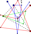
(a)

(b)

Figure 1: LABEL:sub@fig:colcara:conv Example of the convex version of Theorem 1.1 in two dimensions. LABEL:sub@fig:colcara:cone Example of the cone version of Theorem 1.1 in two dimensions.

Theorem 1.1 (Colorful Carathéodory Theorem, Cone Version [4]).

Let $C_{1},\dots,C_{d}\subset\mathbb{R}^{d}$ be point sets and ${\boldsymbol{b}}\in\mathbb{R}^{d}$ a point with ${\boldsymbol{b}}\in\operatorname{pos}(C_{i})$, for $i=1,\dots,d$. Then, there is a colorful choice $C$ for $C_{1},\dots,C_{d}$ that ray-embraces ${\boldsymbol{b}}$. ∎

The classic (convex) version of the colorful Carathéodory theorem follows easily from Theorem 1.1: lift the sets $C_{1},\dots,C_{d+1}\subset\mathbb{R}^{d}$ to $\mathbb{R}^{d+1}$ by appending a $1$ to each element, and set ${\boldsymbol{b}}=(0,\dots,0,1)^{T}$. See Figure 1 for an example of both versions in two dimensions.

Even though the cone version of the colorful Carathéodory theorem guarantees the existence of a colorful choice that ray-embraces the point ${\boldsymbol{b}}$, it is far from clear how to find it efficiently. We call this computational problem the colorful Carathéodory problem (ColorfulCarathéodory). To this day, settling the complexity of ColorfulCarathéodory remains an intriguing open problem, with a potentially wide range of consequences. We can use linear programming to check in polynomial time whether a given colorful choice ray-embraces a point, so ColorfulCarathéodory lies in total function NP (TFNP) [23], the complexity class of total search problems that can be solved in non-deterministic polynomial time. This implies that ColorfulCarathéodory cannot be NP-hard unless $\textsf{NP}=\textsf{coNP}$ [12]. However, the complexity landscape inside TFNP is far from understood, and there exists a rich body of work that studies subclasses of TFNP meant to capture different aspects of mathematical existence proofs, such as the pigeonhole principle (PPP), potential function arguments (PLS, CLS), or various parity arguments (PPAD, PPA, PPADS) [10, 12, 23].

While the complexity of ColorfulCarathéodory remains elusive, related problems are known to be complete for PPAD or for PLS. For example, given $d+1$ point sets $C_{1},\dots,C_{d+1}\subset\mathbb{Q}^{d}$ consisting of two points each and a colorful choice $C$ for $C_{1},\dots,C_{d+1}$ that embraces the origin, it is PPAD-complete to find another colorful choice that embraces the origin [20]. Furthermore, given $d+1$ point sets $C_{1},\dots,C_{d+1}\subset\mathbb{Q}^{d}$, we call a colorful choice $C$ for $C_{1},\dots,C_{d+1}$ locally optimal if the $L_{1}$-distance of $\operatorname{conv}(C)$ to the origin cannot be decreased by swapping a point of color $i$ in $C$ with another point from the same color. Then, computing a locally optimal colorful choice is PLS-complete [22].

Understanding the complexity of ColorfulCarathéodory becomes even more interesting in the light of the fact that the colorful Carathéodory theorem plays a crucial role in proving several other prominent theorems in convex geometry, such as Tverberg’s theorem [25] (and hence the centerpoint theorem [24]) and the first selection lemma [16, 4]. In fact, these proofs can be interpreted as polynomial time reductions from the respective computational problems, Tverberg, Centerpoint, and SimplicialCenter, to ColorfulCarathéodory. See Section A for more details.

Several approximation algorithms have been proposed for ColorfulCarathéodory. Bárány and Onn [5] describe an exact algorithm that can be stopped early to find a colorful choice whose convex hull is “close” to the origin. More precisely, let $\varepsilon,\rho>0$ be parameters. We call a set $\varepsilon$-close if its convex hull has $L_{2}$-distance at most $\varepsilon$ to the origin. Given sets $C_{1},\dots,C_{d+1}\subset\mathbb{R}^{d}$ such that (i) each $C_{i}$ contains a ball of radius $\rho$ centered at the origin in its convex hull; and (ii) all points ${\boldsymbol{p}}\in\bigcup_{i=1}^{d+1}C_{i}$ fulfill $1\leq\|{\boldsymbol{p}}\|\leq 2$ and can be encoded using $L$ bits, one can find an $\varepsilon$-close colorful choice in time $O(\text{poly}(L,\log(1/\varepsilon),1/\rho))$ on the Word-Ram with logarithmic costs. For $\varepsilon=0$, the algorithm actually finds a solution to ColorfulCarathéodory in finite time, and, more interestingly, if $1/\rho=O(\text{poly}(L))$, the algorithm finds a solution to ColorfulCarathéodory in polynomial time. In the same spirit, Barman [6] showed that if the points have constant norm, an $\varepsilon$-close colorful choice can be found by solving $d^{O(1/\varepsilon^{2})}$ convex programs. Mulzer and Stein [22] considered a different notion of approximation: a set is called $m$-colorful if it contains at most $m$ points from each $C_{i}$. They showed that for all fixed $\varepsilon>0$, an $\lceil\varepsilon d\rceil$-colorful choice that contains the origin in its convex hull can be found in polynomial time.

Our Results.

We provide a new upper bound on the complexity of ColorfulCarathéodory by showing that the problem is contained in $\textsf{PPAD}\cap\textsf{PLS}$, implying the first nontrivial upper bound on the computational complexity of computing centerpoints or finding Tverberg partitions.

The traditional proofs of the colorful Carathéodory theorem all proceed through a potential function argument. Thus, it may not be surprising that ColorfulCarathéodory lies in PLS, even though a detailed proof that can deal with degenerate instances requires some care (see Section C). On the other hand, showing that ColorfulCarathéodory lies in PPAD calls for a completely new approach. Even though there are proofs of the colorful Carathéodory theorem that use topological methods usually associated with PPAD (such as certain variants of Sperner’s lemma) [11, 13], these proofs involve existential arguments that have no clear algorithmic interpretation. Thus, we present a new proof of the colorful Carathéodory theorem that proceeds similarly as the usual proof for Sperner’s lemma [8]. This new proof has an algorithmic interpretation that leads to a formulation of ColorfulCarathéodory as a PPAD-problem.

Finally, we consider the special case of ColorfulCarathéodory that we are given two color classes $C_{1},C_{2}\subset\mathbb{R}^{d}$ of $d$ points each and a vector ${\boldsymbol{b}}\in\mathbb{R}^{d}$ such that both $C_{1}$ and $C_{2}$ ray-embrace ${\boldsymbol{b}}$. We describe an algorithm that solves the following problem in polynomial time: given $k\in[d]$, find a set $C\subseteq C_{1}\cup C_{2}$ with $|C\cap C_{1}|=k$ and $|C\cap C_{2}|=d-k$ such that $C$ ray-embraces ${\boldsymbol{b}}$. Note that this is a special case of ColorfulCarathéodory since we can just take $k$ copies of $C_{1}$ and $d-k$ copies of $C_{2}$ in a problem instance for ColorfulCarathéodory.

2 Preliminaries

The Complexity Class PPAD.

The complexity class polynomial parity argument in a directed graph (PPAD) [23] is a subclass of TFNP that contains search problems that can be modeled as follows: let $G=(V,E)$ be a directed graph in which each node has indegree and outdegree at most one. That is, $G$ consists of paths and cycles. We call a node $v\in V$ a source if $v$ has indegree $0$ and we call $v$ a sink if it has outdegree $0$. Given a source in $G$, we want to find another source or sink. By a parity argument, there is an even number of sources and sinks in $G$ and hence another source or sink must exist. However, finding this sink or source is nontrivial since $G$ is defined implicitly and the total number of nodes may be exponential.

More formally, a problem in PPAD is a relation $\mathcal{R}$ between a set $\mathcal{I}\subseteq\{0,1\}^{\star}$ of problem instances and a set $\mathcal{S}\subset\{0,1\}^{\star}$ of candidate solutions. Assume further the following.

• The set $\mathcal{I}$ is polynomial-time verifiable. Furthermore, there is an algorithm that on input $I\in\mathcal{I}$ and $s\in\mathcal{S}$ decides in time $\operatorname{poly}(|I|)$ whether $s$ is a valid candidate solution for $I$. We denote with $\mathcal{S}_{I}\subseteq\mathcal{S}$ the set of all valid candidate solutions for a fixed instance $I$.

• There exist two polynomial-time computable functions $\operatorname{pred}$ and $\operatorname{succ}$ that define the edge set of $G$ as follows: on input $I\in\mathcal{I}$ and $s\in\mathcal{S}_{I}$, $\operatorname{pred}$ and $\operatorname{succ}$ return a valid candidate solution from $\mathcal{S}_{I}$ or $\bot$. Here, $\bot$ means that $v$ has no predecessor/successor.

• There is a polynomial-time algorithm that returns for each instance $I$ a valid candidate solution $s\in\mathcal{S}_{I}$ with $\operatorname{pred}(s)=\bot$. We call $s$ the standard source.

Now, each instance $I\in\mathcal{I}$ defines a graph $G_{I}=(V,E)$ as follows. The set of nodes $V$ is the set of all valid candidate solutions $\mathcal{S}_{I}$ and there is a directed edge from $u$ to $v$ if and only if $v=\operatorname{succ}(u)$ and $u=\operatorname{pred}(v)$. Clearly, each node in $G_{I}$ has indegree and outdegree at most one. The relation $\mathcal{R}$ consists of all tuples $(I,s)$ such that $s$ is a sink or source other than the standard source in $G_{I}$.

The definition of a PPAD-problem suggests a simple algorithm, called the standard algorithm: start at the standard source and follow the path until a sink is reached. This algorithm always finds a solution but the length of the traversed path may be exponential in the size of the input instance.

Polyhedral Complexes and Subdivisions.

We call a finite set of polyhedra $\mathcal{P}$ in $\mathbb{R}^{d}$ a polyhedral complex if and only if (i) for all polyhedra $f\in\mathcal{P}$, all faces of $f$ are contained in $\mathcal{P}$; and (ii) for all $f,f^{\prime}\in\mathcal{P}$, the intersection $f\cap f^{\prime}$ is a face of both. Note that the first requirement implies that $\emptyset\in\mathcal{P}$. Furthermore, we say $\mathcal{P}$ has dimension $k$ if there exists some polyhedron $f\in\mathcal{P}$ with $\dim f=k$ and all other polyhedra in $\mathcal{P}$ have dimension at most $k$. We call $\mathcal{P}$ a polytopal complex if it is a polyhedral complex and all elements are polytopes. Similarly, we say $\mathcal{P}$ is a simplicial complex if it is a polytopal complex whose elements are simplices. Finally, we say $\mathcal{P}$ subdivides a set $Q\subseteq\mathbb{R}^{d}$ if $\bigcup_{f\in\mathcal{P}}f=Q$. For more details, see [27, Section 5.1].

Linear Programming.

Let $A\in\mathbb{R}^{d\times n}$ be a matrix and $F$ a set of column vectors from $A$. Then, we denote with ${\operatorname{ind}\left(F\right)}\subseteq[n]$ the set of column indices in $F$ and for an index set $I\subseteq[n]$, we denote with $A_{I}$ the submatrix of $A$ that consists of the columns indexed by $I$. Similarly, for a vector ${\boldsymbol{c}}\in\mathbb{R}^{n}$ and an index set $I\subset[n]$, we denote with ${\boldsymbol{c}}_{I}$ the subvector of ${\boldsymbol{c}}$ with the coordinates indexed by $I$. Now, let $L^{\prime}$ denote a system of linear equations

$$L^{\prime}:A{\boldsymbol{x}}={\boldsymbol{b}},$$

where $A\in\mathbb{Q}^{d\times n}$, ${\boldsymbol{b}}\in\mathbb{Q}^{d}$ and $\operatorname{rank}(A)=k$. By multiplying with the least common denominator, we may assume in the following that $A\in\mathbb{Z}^{d\times n}$ and ${\boldsymbol{b}}\in\mathbb{Z}^{d}$. We call a set of $k$ linearly independent column vectors $B$ of $A$ a basis and we say that $A$ is non-degenerate if $k=d$ and for all bases $B$ of $A$, no coordinate of the corresponding solution ${\boldsymbol{x}}_{{\operatorname{ind}\left(B\right)}}$ is $0$. In particular, if $L^{\prime}$ is non-degenerate, then ${\boldsymbol{b}}$ is not contained in the linear span of any set of $d^{\prime}<d$ column vectors from $A$ and hence if $d>n$, the linear system $L^{\prime}$ has no solution. In the following, we assume that $L^{\prime}$ is non-degenerate and that $d\leq n$.

We denote with $L$ the linear program obtained by extending the linear system $L^{\prime}$ with the constraints ${\boldsymbol{x}}\geq{\boldsymbol{0}}$ and with a cost vector ${\boldsymbol{c}}\in\mathbb{Q}^{n}$:

$$L:\min{\boldsymbol{c}}^{T}{\boldsymbol{x}}\text{ subject to }A{\boldsymbol{x}}={\boldsymbol{b}},\,{\boldsymbol{x}}\geq{\boldsymbol{0}}.$$

We say a set of column vectors $B$ is a basis for $L$ if $B$ is a basis for $L^{\prime}$. Let ${\boldsymbol{x}}\in\mathbb{R}^{n}$ be the corresponding solution, i.e., let ${\boldsymbol{x}}$ be such that $A{\boldsymbol{x}}={\boldsymbol{b}}$ and $x_{i}=0$ for $i\in[n]\setminus{\operatorname{ind}\left(B\right)}$. We call ${\boldsymbol{x}}$ a basic feasible solution, and $B$ a feasible basis, if ${\boldsymbol{x}}\geq{\boldsymbol{0}}$. Furthermore, we say $L$ is non-degenerate if for all feasible bases $B$, the corresponding basic feasible solutions have strictly positive values in the coordinates of $B$. Now, let $R=[n]\setminus{\operatorname{ind}\left(B\right)}$ be the column indices not in $B$. The reduced cost vector ${\boldsymbol{r}}_{B,{\boldsymbol{c}}}\in\mathbb{Q}^{n-d}$ with respect to $B$ and ${\boldsymbol{c}}$ is then defined as

$${\boldsymbol{r}}_{B,{\boldsymbol{c}}}={\boldsymbol{c}}_{R}-\left(A^{-1}_{\operatorname{ind}\left(B\right)}A_{R}\right)^{T}{\boldsymbol{c}}_{\operatorname{ind}\left(B\right)}.$$ (1)

It is well-known that $B$ is optimal for ${\boldsymbol{c}}$ if and only if ${\boldsymbol{r}}_{B,{\boldsymbol{c}}}$ is non-negative in all coordinates [18]. For technical reasons, we consider in the following the extended reduced cost vector ${\hat{{\boldsymbol{r}}}}_{B,{\boldsymbol{c}}}\in\mathbb{Q}^{n}$ that has a $0$ in dimensions ${\operatorname{ind}\left(B\right)}$ and otherwise equals ${\boldsymbol{r}}_{B,{\boldsymbol{c}}}$ to align the coordinates of the reduced cost vector with the column indices in $A$. More formally, we set

$$\left({\hat{{\boldsymbol{r}}}}_{B,{\boldsymbol{c}}}\right)_{j}=\begin{cases}0&\text{if }j\in{\operatorname{ind}\left(B\right)}\text{, and}\\ ({\boldsymbol{r}}_{B,{\boldsymbol{c}}})_{j^{\prime}}&\text{otherwise,}\end{cases}$$

where $j^{\prime}$ is the rank of $j$ in $R$, that is, $({\boldsymbol{r}}_{B,{\boldsymbol{c}}})_{j^{\prime}}$ is the coordinate of ${\boldsymbol{r}}_{B,{\boldsymbol{c}}}$ that corresponds to the $j^{\prime}$th non-basis column with column index $j$ in $A$.

Geometrically, the feasible solutions for the linear program $L$ define an $(n-d)$-dimensional polyhedron $\mathcal{P}$ in $\mathbb{R}^{n}$. Since $L$ is non-degenerate, $\mathcal{P}$ is simple. Let $f\subseteq\mathcal{P}$ be a $k$-face of $\mathcal{P}$. Then, $f$ has an associated set ${\operatorname{supp}\left(f\right)}\subseteq[n]$ of $k$ column indices such that $f$ consists precisely of the feasible solutions for the linear program $A_{\operatorname{supp}\left(f\right)}{\boldsymbol{x}}^{\prime}={\boldsymbol{b}},\,{\boldsymbol{x}}^{\prime}\geq{\boldsymbol{0}}$, lifted to $\mathbb{R}^{n}$ by setting the coordinates with indices not in ${\operatorname{supp}\left(f\right)}$ to $0$. We call ${\operatorname{supp}\left(f\right)}$ the support of $f$ and we say the columns in $A_{\operatorname{supp}\left(f\right)}$ define $f$. Furthermore, for all subfaces $\check{f}\subseteq f$, we have ${\operatorname{supp}\left(\check{f}\right)}\subseteq{\operatorname{supp}\left(f\right)}$ and in particular, all bases that define vertices of $f$ are $d$-subsets of columns from $A_{\operatorname{supp}\left(f\right)}$.

Moreover, we say a nonempty face $f\subseteq\mathcal{P}$ is optimal for a cost vector ${\boldsymbol{c}}$ if all points in $f$ are optimal for ${\boldsymbol{c}}$. We can express this condition using the reduced cost vector. Let $B$ be a basis for a vertex in $f$. Then $f$ is optimal for ${\boldsymbol{c}}$ if and only if

$$({\hat{{\boldsymbol{r}}}}_{B,{\boldsymbol{c}}})_{j}=0\text{\leavevmode\nobreak\ for $j\in{\operatorname{supp}\left(f\right)}$, and }({\hat{{\boldsymbol{r}}}}_{B,{\boldsymbol{c}}})_{j}\leq 0\text{\leavevmode\nobreak\ otherwise.}$$

3 Overview of the PPAD-Formulation

We give a new constructive proof of the cone version of the colorful Carathéodory theorem based on Sperner’s lemma. Using this, we can obtain a PPAD-formulation of ColorfulCarathéodory, by adapting Papadimitriou’s formulation of Sperner’s lemma as a PPAD problem.

Recall the statement of Sperner’s lemma: let $\mathcal{S}$ be a simplicial subdivision of the $d$-dimensional standard simplex $\Delta^{d}=\operatorname{conv}({\boldsymbol{e}}_{1},\dots,{\boldsymbol{e}}_{d+1})\subset\mathbb{R}^{d+1}$, where ${\boldsymbol{e}}_{i}$ is the $i$th canonical basis vector. We call a function $\lambda$ that assigns to each vertex in $\mathcal{S}$ a label from $[d+1]$ a Sperner labeling if for each vertex ${\boldsymbol{v}}$ of $\mathcal{S}$ contained in $\operatorname{conv}({\boldsymbol{e}}_{i_{1}},\dots,{\boldsymbol{e}}_{i_{k}})$, we have $\lambda({\boldsymbol{v}})\in\{i_{1},\dots,i_{k}\}$, for all $\{i_{1},\dots,i_{k}\}\subseteq[d+1],k\in[d+1]$. For a simplex $\sigma\in\mathcal{S}$, we set $\lambda(\sigma)$ to be the set of labels of the vertices of $\sigma$. We call $\sigma$ fully-labeled if $\lambda(\sigma)=[d+1]$.

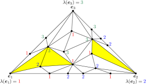
Figure 2: An example of Sperner’s lemma in two dimensions. The fully-labeled simplices are marked yellow.

Theorem 3.1 (Strong Sperner’s Lemma [8]).

The number of fully-labeled simplices is odd.

Now suppose we are given an instance $I=(C_{1},\dots,C_{d},{\boldsymbol{b}})$ of (the cone version of) ColorfulCarathéodory, where ${\boldsymbol{b}}\in\mathbb{R}^{d}$, ${\boldsymbol{b}}\neq{\boldsymbol{0}}$, and each $C_{i}\subset\mathbb{Q}^{d}$, $i\in[d]$, ray-embraces ${\boldsymbol{b}}$. In Section B, we show that we can assume w.l.o.g. that each set $C_{i}$ has size $d$. We now describe how to define a simplicial complex $\mathcal{S}$ and a Sperner labeling $\lambda$ for $I$ such that a fully labeled simplex will encode a colorful choice that contains the vector ${\boldsymbol{b}}$ in its positive span.

In the following, we call $\mathbb{R}^{d}$ the parameter space and a vector ${\boldsymbol{\mu}}\in\mathbb{R}^{d}$ a parameter vector. We define a family of linear programs $\{L^{\textsc{CC}}_{\boldsymbol{\mu}}\mid{\boldsymbol{\mu}}\in\mathbb{R}^{d}\}$, where each linear program $L^{\textsc{CC}}_{\boldsymbol{\mu}}$ has the same constraints and differs only in its cost vector ${\boldsymbol{c}}_{\boldsymbol{\mu}}$. The cost vector ${\boldsymbol{c}}_{\boldsymbol{\mu}}$ is defined by a linear function in ${\boldsymbol{\mu}}\in\mathbb{R}^{d}$. Let $A=(C_{1}\;C_{2}\;\dots\;C_{d})\in\mathbb{Q}^{d\times d^{2}}$ be the matrix that has the vectors from $C_{1}$ in the first $d$ columns, the vectors from $C_{2}$ in the second $d$ columns, and so on. Then, we denote with $L^{\textsc{CC}}_{{\boldsymbol{\mu}}}$ the linear program

$$L^{\textsc{CC}}_{{\boldsymbol{\mu}}}:\min{\boldsymbol{c}}^{T}_{{\boldsymbol{\mu}}}{\boldsymbol{x}},\,\text{ subject to }A{\boldsymbol{x}}={\boldsymbol{b}},{\boldsymbol{x}}\geq{\boldsymbol{0}},$$ (2)

and we denote with $\mathcal{P}^{\textsc{CC}}\subset\mathbb{R}^{d^{2}}$ the polyhedron that is defined by the linear system $L^{\textsc{CC}}$. We can think of the $i$th coordinate of the parameter vector ${\boldsymbol{\mu}}\in\mathbb{R}^{d}$ as the weight of color $i$, i.e., the costs of columns from $A$ with color $i$ decrease if $({\boldsymbol{\mu}})_{i}$ increases. To each face $f$ of $P$, we assign the set of parameter vectors $\Phi(f)\subset\mathbb{R}^{d}$ such that for all ${\boldsymbol{\mu}}\in\Phi(f)$, the face $f$ is optimal for the linear program $L^{\textsc{CC}}_{\boldsymbol{\mu}}$ that has $L^{\textsc{CC}}$ as constraints and ${\boldsymbol{c}}_{\boldsymbol{\mu}}$ as cost vector. We call $\Phi(f)$ the parameter region of $f$. The cost vector is designed to control the colors that appear in the support of optimal faces for a specific subset of parameter vectors. Let $\mathcal{M}=\left\{{\boldsymbol{\mu}}\in\mathbb{R}^{d}\,\middle|\,{\boldsymbol{\mu}}\geq{\boldsymbol{0}},\,\|{\boldsymbol{\mu}}\|_{\infty}=1\right\}$ denote the faces of the unit cube in which at least one coordinate is set to $1$. Then, no face $f$ that is assigned to a parameter vector ${\boldsymbol{\mu}}\in\mathcal{M}$ with $({\boldsymbol{\mu}})_{i^{\times}}=0$ has a column from $A$ with color $i^{\times}$ in its defining set $A_{\operatorname{supp}\left(f\right)}$. This property will become crucial when we define a Sperner labeling later on. Now, we define a polyhedral subcomplex $\mathcal{F}$ of $\mathcal{P}^{\textsc{CC}}$ that consists of all faces $f$ of $\mathcal{P}^{\textsc{CC}}$ such that $\Phi(f)\cap\mathcal{M}\neq\emptyset$. Furthermore, the intersections of the parameter regions with $\mathcal{M}$ induce a polytopal complex $\mathcal{Q}$ that is in a dual relationship to $\mathcal{F}$. By performing a central projection with the origin as center of $\mathcal{Q}$ onto the standard simplex $\Delta^{d-1}$, we obtain a polytopal subdivision $\mathcal{Q}_{\Delta}$ of $\Delta^{d-1}$. To get the desired simplicial subdivision of $\Delta^{d-1}$, we take the barycentric subdivision $\operatorname{sd}\mathcal{Q}_{\Delta}$ of $\mathcal{Q}_{\Delta}$.

We construct a Sperner labeling $\lambda$ for $\operatorname{sd}\mathcal{Q}_{\Delta}$ as follows: let ${\boldsymbol{v}}$ be a vertex in $\operatorname{sd}\mathcal{Q}_{\Delta}$, and let $f$ be the face of $\mathcal{F}$ that corresponds to ${\boldsymbol{v}}$. Then, we set $\lambda({\boldsymbol{v}})=i$ if the $i$th color appears most often in the support of $f$. The color controlling property of the cost function $c_{\boldsymbol{\mu}}$ then implies that $\lambda$ is a Sperner labeling. Furthermore, using the properties of the barycentric subdivision and the correspondence between $\mathcal{Q}_{\Delta}$ and $\mathcal{F}$, we can show that one vertex of a fully-labeled $(d-1)$-simplex in $\operatorname{sd}\mathcal{Q}_{\Delta}$ encodes a colorful feasible basis of the ColorfulCarathéodory instance $I$. This concludes a new constructive proof of the colorful Carathéodory theorem using Sperner’s lemma.

To show that ColorfulCarathéodory is in PPAD however, we need to be able to traverse $\operatorname{sd}\mathcal{Q}_{\Delta}$ efficiently. For this, we introduce a combinatorial encoding of the simplices in $\mathcal{Q}_{\Delta}$ that represents neighboring simplices in a similar manner. Furthermore, we describe how to generalize the orientation used in the PPAD formulation of 2D-Sperner [23] to our setting. This finally shows that ColorfulCarathéodory is in PPAD.

To ensure that the complexes that appear in our algorithms are sufficiently generic, we prove several perturbation lemmas that give a deterministic way of achieving this. Our PPAD-formulation also shows that the special case of ColorfulCarathéodory involving two colors can be solved in polynomial time. Indeed, we will see that in this case the polytopal complex $\mathcal{Q}_{\Delta}$ can be made $1$-dimensional. Then, binary search can be used to find a fully-labeled simplex in $\mathcal{Q}_{\Delta}$. In order to prove that the binary search terminates after a polynomial number of steps, we use methods similar to our perturbation techniques to obtain a bound on the length of the $1$-dimensional fully-labeled simplex.

4 The Colorful Carathéodory Problem is in PPAD

As before, let $I=(C_{1},\dots,C_{d},{\boldsymbol{b}})$ denote an instance for the cone version of ColorfulCarathéodory. Our formulation of ColorfulCarathéodory as a PPAD-problem requires $I$ to be in general position. In particular, we assume that (P1) all color classes $C_{i}\subset\mathbb{Z}^{d}$ consist of $d$ points and all points have integer coordinates. Furthermore, we assume that (P2) there exist no subset $P\subset\bigcup_{i=1}^{d}C_{i}$ of size $d-1$ that ray-embraces ${\boldsymbol{b}}$. We show in Section B how to ensure the properties by an explicit deterministic perturbation of polynomial bit-complexity.

4.1 The Polytopal Complex

Let $N=d!m^{d}$, where $m$ is the largest absolute value that appears in $A$ and ${\boldsymbol{b}}$ (see Lemma D.1). Then, we define ${\boldsymbol{c}}_{{\boldsymbol{\mu}}}\in\mathbb{R}^{d^{2}}$ as

$$({\boldsymbol{c}}_{{\boldsymbol{\mu}}})_{j}=1+\left(1-({\boldsymbol{\mu}})_{i}\right)dN^{2}+\varepsilon^{j},$$ (3)

where $j\in[d^{2}]$, $i$ is the color of the $j$th column in $A$, and $0<\varepsilon\leq N^{-3}$ is a suitable perturbation that ensures non-degeneracy of the reduced costs (see [7]). As stated in the overview, the cost function controls the colors in the support of the optimal faces for parameter vectors in $\mathcal{M}$. The proof of the following lemma can be found in Section D.

Lemma 4.1.

Let $i^{\times}\in[d]$ be a color and let ${\boldsymbol{\mu}}\in\mathcal{M}$ be a parameter vector with ${\boldsymbol{\mu}}_{i^{\times}}=0$. Furthermore, let $B^{\star}$ be an optimal feasible basis for $L^{\textsc{CC}}_{\boldsymbol{\mu}}$. Then, $B^{\star}\cap C_{i^{\times}}=\emptyset$.

We denote for a face $f\subseteq\mathcal{P}^{\textsc{CC}}$, $f\neq\emptyset$, with $\Phi(f)=\big{\{}{\boldsymbol{\mu}}\in\mathbb{R}^{d}\mid\text{$f$ is optimal for $L_{{\boldsymbol{\mu}}}$}\big{\}}$ the set of all parameter vectors for which $f$ is optimal. We call this the parameter region for $f$. Using the reduced cost vector, we can express $\Phi(f)$ as solution space to the following linear system, where $B$ is a feasible basis of some vertex of $f$ and the $d$ coordinates of the parameter vector ${\boldsymbol{\mu}}$ are the variables:

$$L^{\Phi}_{B,f}:({\hat{{\boldsymbol{r}}}}_{B,{\boldsymbol{c}}_{\boldsymbol{\mu}}})_{j}=0\text{\ for }j\in{\operatorname{supp}\left(f\right)}\setminus{\operatorname{ind}\left(B\right)}\text{ and }({\hat{{\boldsymbol{r}}}}_{B,{\boldsymbol{c}}_{\boldsymbol{\mu}}})_{j}\leq 0\text{\ for }\big{[}d^{2}\big{]}\setminus{\operatorname{supp}\left(f\right)}.$$ (4)

Then, we define $\mathcal{F}$ as the set of all faces that are optimal for some parameter vector in $\mathcal{M}$:

$$\mathcal{F}=\left\{f\,\middle|\,\text{$f$ is a face of $\mathcal{P}^{\textsc{CC}}$},\,\Phi(f)\cap\mathcal{M}\neq\emptyset\right\}.$$

By definition, $\mathcal{F}\cup\{\emptyset\}$ is a polyhedral subcomplex of $\mathcal{P}^{\textsc{CC}}$. The intersections of the parameter regions with faces of $\mathcal{M}$ induce a subdivision $\mathcal{Q}$ of $\mathcal{M}$:

$$\mathcal{Q}=\left\{\Phi(f)\cap g\,\middle|\,f\in\mathcal{F},\,\text{$g$ is a face of $\mathcal{M}$}\right\}.$$

In Section D, we show that $\mathcal{Q}$ is a $(d-1)$-dimensional polytopal complex. Next, we construct $\mathcal{Q}_{\Delta}$ through a central projection with the origin as center of $\mathcal{Q}$ onto the $(d-1)$-dimensional standard simplex $\Delta\subset\mathbb{R}^{d}$. It is easy to see that this projection is a bijection. For a parameter vector ${\boldsymbol{\mu}}\in\mathbb{R}^{d}$, we denote with $\Delta({\boldsymbol{\mu}})={\boldsymbol{\mu}}/\|{\boldsymbol{\mu}}\|_{1}$ its projection onto $\Delta$. Similarly, we denote with $\mathcal{M}({\boldsymbol{\mu}})={\boldsymbol{\mu}}/\|{\boldsymbol{\mu}}\|_{\infty}$ the projection of ${\boldsymbol{\mu}}$ onto $\mathcal{M}$ and we use the same notation to denote the element-wise projection of sets. Then, we can write the projection $\mathcal{Q}_{\Delta}$ of $\mathcal{Q}$ onto $\Delta$ as $\mathcal{Q}_{\Delta}=\{\Delta(q)\mid q\in\mathcal{Q}\}$. Furthermore, let $\SS=\{\Delta(g)\mid\text{$g$ is a face of $\mathcal{M}$}\}$ denote the projections of the faces of $\mathcal{M}$ onto $\Delta$. For $f\in\mathcal{F}$, let $\Phi_{\Delta}(f)=\Delta(\Phi(f)\cap\mathcal{M})$ denote the projection of all parameter vectors in $\mathcal{M}$ for which $f$ is optimal onto $\Delta$. Please refer to Table 1 on Page 1 for an overview of the current and future notation. The following results are proved in Section D.

Lemma 4.2.

Let $q\neq\emptyset$ be an element from $\mathcal{Q}_{\Delta}$. Then, there exists unique pair $(f,g)$ where $f$ is a face of $\mathcal{F}$ and $g$ is a face of $\SS$ such that $q=\Phi_{\Delta}(f)\cap g$. Moreover, $q$ is a simple polytope of dimension $\dim g-\dim f$ and, if $\dim q>0$, the set of facets of $q$ can be written as

$$\left.\Big{\{}\Phi_{\Delta}\left(f\right)\cap\check{g}\neq\emptyset\,\middle|\,\text{$\check{g}$ is a facet of $g$}\Big{\}}\right.\cup\left\{\Phi_{\Delta}\left({\hat{f}}\right)\cap g\neq\emptyset\,\middle|\,\text{$f$ is a facet of ${\hat{f}}\in\mathcal{F}$}\right\}.$$

Lemma 4.3.

The set $\mathcal{Q}_{\Delta}$ is a $(d-1)$-dimensional polytopal complex that decomposes $\Delta$. ∎

4.2 The Barycentric Subdivision

The barycentric subdivision [17, Definition 1.7.2] is a well-known method to subdivide a polytopal complex into simplices. We define $\operatorname{sd}\mathcal{Q}_{\Delta}$ as the set of all simplices $\operatorname{conv}({\boldsymbol{v}}_{0},\dots,{\boldsymbol{v}}_{k})$, $k\in[d]$, such that there exists a chain $q_{0}\subset\dots\subset q_{k}$ of polytopes in $\mathcal{Q}_{\Delta}$ with $\dim q_{i-1}<\dim q_{i}$ and such that ${\boldsymbol{v}}_{i}$ is the barycenter of $q_{i}$ for $i\in[k]$. We define the label of a vertex ${\boldsymbol{v}}\in\operatorname{sd}\mathcal{Q}_{\Delta}$ as follows. By Lemma 4.2, there exists a unique pair $f\in\mathcal{F}$ and $g\in\SS$ with ${\boldsymbol{v}}=\Phi_{\Delta}(f)\cap g$. Then, the label $\lambda({\boldsymbol{v}})$ of ${\boldsymbol{v}}$ is defined as

$$\lambda({\boldsymbol{v}})=\operatorname*{arg\,max}_{i\in[d]}\left|{\operatorname{ind}\left(C\right)}_{i}\cap{\operatorname{supp}\left(f\right)}\right|.$$ (5)

In case of a tie, we take the smallest $i\in[d]$ that achieves the maximum. Lemma 4.1 implies that $\lambda(\cdot)$ is a Sperner labeling of $\operatorname{sd}\mathcal{Q}_{\Delta}$. In fact, $\lambda$ is a Sperner labeling for any fixed simplicial subdivision of $\Delta$. Now, Theorem 3.1 guarantees the existence of a $(d-1)$-simplex $\sigma\in\operatorname{sd}\mathcal{Q}_{\Delta}$ whose vertices have all $d$ possible labels. The next lemma shows that then one of the vertices of $\sigma$ defines a solution to the ColorfulCarathéodory instance. Here, we use specific properties of the barycentric subdivision.

Lemma 4.4.

Let $\sigma\in\operatorname{sd}\mathcal{Q}_{\Delta}$ be a fully-labeled $(d-1)$-simplex and let ${\boldsymbol{v}}_{d-1}$ denote the vertex of $\sigma$ that is the barycenter of a $(d-1)$-face $q_{d-1}=\Phi_{\Delta}(f_{d-1})\cap g_{d-1}\in\mathcal{Q}_{\Delta}$, where $f_{d-1}\in\mathcal{F}$ and $g_{d-1}\in\SS$. Then, the columns from $A_{{\operatorname{supp}\left(f_{d-1}\right)}}$ are a colorful choice that ray-embraces ${\boldsymbol{b}}$.

Our discussion up to now already yields a new Sperner-based proof of the colorful Carathéodory theorem. However, in order to show that $\textsc{ColorfulCarath\'{e}odory}\in\textsf{PPAD}$, we need to replace the invocation of Theorem 3.1 by a PPAD-problem. Note that it is not possible to use the formulation of Sperner from [23, Theorem 2] directly, since it is defined for a fixed simplicial subdivision of the standard simplex. In our case, the simplicial subdivision of $\Delta$ depends on the input instance. In the following, we generalize the PPAD formulation of Sperner in [23] to $\mathcal{Q}_{\Delta}$ by mimicking the proof of Theorem 3.1. For this, we need to be able to find simplices in $\operatorname{sd}\mathcal{Q}_{\Delta}$ that share a given facet. We begin with a simple encoding of simplices in $\operatorname{sd}\mathcal{Q}_{\Delta}$ that allows us to solve this problem completely combinatorially.

We first show how to encode a polytope $q\in\mathcal{Q}_{\Delta}$. By Lemma 4.2, there exists a unique pair of faces $f\in\mathcal{F}$ and $g\in S$ such that $q=\Phi_{\Delta}(f)\cap g$. Since $\mathcal{M}(g)$ is a face of the unit cube, the value of $d-\dim g$ coordinates in $\mathcal{M}(g)$ is fixed to either $0$ or $1$. Let $I_{j}\subseteq[d]$, $j=0,1$, denote the indices of the coordinates that are fixed to $j$. Then, the encoding of $q$ is defined as ${\operatorname{enc}\left(q\right)}=\left({\operatorname{supp}\left(f\right)},I_{0},I_{1}\right)$. We use this to define an encoding of the simplices in $\mathcal{Q}_{\Delta}$ as follows. Let $\sigma\in\mathcal{Q}_{\Delta}$ be a $k$-simplex and let $q_{0}\subset\dots\subset q_{k}$ be the corresponding face chain in $\mathcal{Q}_{\Delta}$ such that the $i$th vertex of $\sigma$ is the barycenter of $q_{i}$. Then, the encoding ${\operatorname{enc}\left(\sigma\right)}$ is defined as

$${\operatorname{enc}\left(\sigma\right)}=\left({\operatorname{enc}\left(q_{0}\right)},\dots,{\operatorname{enc}\left(q_{k}\right)}\right).$$ (6)

In the proof of Theorem 3.1, we traverse only a subset of simplices in the simplicial subdivision, namely $(k-1)$-simplices that are contained in the face $\Delta_{[k]}=\operatorname{conv}\{{\boldsymbol{e}}_{i}\mid i\in[k]\}$ of $\Delta$ for $k\in[d]$. Let $\Sigma_{k}=\left\{\sigma\in\operatorname{sd}\mathcal{Q}_{\Delta}\,\middle|\,\dim(\sigma)=k-1,\ \sigma\subseteq\Delta_{[k]}\right\}$ denote the set of $(k-1)$-simplices in $\operatorname{sd}\mathcal{Q}_{\Delta}$ that are contained in the $(k-1)$-face, where $k\in[d]$, and let $\Sigma=\bigcup_{k=1}^{d}\Sigma_{k}$ be the collection of all those simplices. In the following, we give a precise characterization of the encodings of the simplices in $\Sigma_{k}$. For two disjoint index sets $I_{0},I_{1}\subseteq[d]$, we denote with $g(I_{0},I_{1})=\left\{{\boldsymbol{\mu}}\in\mathcal{M}\,\middle|\,j=0,1,\,({\boldsymbol{\mu}})_{i}=j\text{ for $i\in I_{j}$}\right\}$ the face of $\mathcal{M}$ that we obtain by fixing the coordinates in dimensions $I_{0}\cup I_{1}$. Let now $T=\left(Q_{0},\dots,Q_{k-1}\right)$, $k\in[d-1]$, be a tuple, where $Q_{i}=\left(S^{(i)},I^{(i)}_{0},I^{(i)}_{1}\right)$, $S^{(i)}\subset\left[d^{2}\right]$, and $I^{(i)}_{0},I^{(i)}_{1}$ are disjoint subsets of $[d]$ with $I^{(i)}_{1}\neq\emptyset$ for $i\in[k-1]_{0}$. We say $T$ is valid if and only if $T$ has the following properties.

1. We have $I^{(k-1)}_{0}=[d]\setminus[k]$, $\left|I^{(k-1)}_{1}\right|=1$, and the columns in $A_{S^{(k-1)}}$ are a feasible basis for a vertex $f$. Moreover, the intersection $\Phi(f)\cap g\left(I^{(k-1)}_{0}\cup I^{(k-1)}_{1}\right)$ is nonempty.

2. For all $i\in[k-1]$, we either have

   1. $I^{(i-1)}_{0}=I^{(i)}_{0}$, $I^{(i-1)}_{1}=I^{(i)}_{1}$, and $S^{(i-1)}=S^{(i)}\cup\left\{a_{i-1}\right\}$ for some index $a_{i-1}\in\left[d^{2}\right]\setminus S^{(i)}$,

   2. or $S^{(i-1)}=S^{(i)}$ and there is an index $j_{i-1}\in[d]\setminus\left(I^{(i)}_{0}\cup I^{(i)}_{1}\right)$ such that either $I^{(i-1)}_{0}=I^{(i)}_{0}$ and $I^{(i-1)}_{1}=I^{(i)}_{1}\cup\left\{j_{i-1}\right\}$, or $I^{(i-1)}_{1}=I^{(i)}_{1}$ and $I^{(i-1)}_{0}=I^{(i)}_{0}\cup\left\{j_{i-1}\right\}$.

Lemma 4.5.

For $k\in[d]$, the function ${\operatorname{enc}\left(\cdot\right)}$ restricted to the simplices in $\Sigma_{k}$ is a bijection from $\Sigma_{k}$ to the set of valid $k$-tuples.

Using our characterization of encodings as valid tuples, it becomes an easy task to check whether a given candidate encoding corresponds to a simplex in $\Sigma$.

Lemma 4.6.

Let $T=\left(Q_{0},\dots,Q_{k-1}\right)$, $k\in[d-1]$, be a tuple, where $Q_{i}=\left(S^{(i)},I^{(i)}_{0},I^{(i)}_{1}\right)$, $S^{(i)}\subset\left[d^{2}\right]$, and $I^{(i)}_{0},I^{(i)}_{1}$ are disjoint subsets of $[d]$ with $I^{(i)}_{1}\neq\emptyset$ for $i\in[k-1]_{0}$. Then, we can check in polynomial time whether $T$ is a valid $k$-tuple.

In Section E, we show that simplices in $\Sigma$ that share a facet have similar encodings that differ only in one element of the encoding tuples. Using this fact, we can traverse $\Sigma$ efficiently by manipulating the respective encodings.

Lemma 4.7.

Let $\sigma\in\Sigma_{k}$ be a simplex and let $q_{0}\subset\dots\subset q_{k-1}$ be the corresponding face chain in $\mathcal{Q}_{\Delta}$ such that the $i$th vertex ${\boldsymbol{v}}_{i}$ of $\sigma$ is the barycenter of $q_{i}$, where $k\in[d]$ and $i\in[k-1]_{0}$. Then, we can solve the following problems in polynomial time: (i) Given ${\operatorname{enc}\left(\sigma\right)}$ and $i$, compute the encoding of the simplex $\sigma^{\prime}\in\Sigma_{k}$ that shares the facet $\operatorname{conv}\left\{{\boldsymbol{v}}_{j}\,\middle|\,j\in[k-1]_{0},\,j\neq i\right\}$ with $\sigma$ or state that there is none; (ii) Assuming that $k<d$ and given ${\operatorname{enc}\left(\sigma\right)}$, compute the encoding of the simplex ${\hat{\sigma}}\in\Sigma_{k+1}$ that has $\sigma$ as facet; and (iii) Assuming that $k>1$ and given ${\operatorname{enc}\left(\sigma\right)}$, compute the encoding of the simplex $\check{\sigma}\in\Sigma_{k-1}$ that is a facet of $\sigma$ or state that there is none.

4.3 The PPAD graph

Using our tools from the previous sections, we now describe the PPAD graph $G=(V,E)$ for the ColorfulCarathéodory instance. The definition of $G$ follows mainly the ideas from the formulation of Sperner as a PPAD-problem [23, Theorem 2] and the proof of Theorem 3.1.

The graph has one node per simplex in $\Sigma$ that has all labels or all but the largest possible label. That is, we have one node for each $(k-1)$-simplex $\sigma$ in $\Sigma_{k}$ with $[k-1]\subseteq\lambda(\sigma)$. Two simplices are connected by an edge if one simplex is the facet of the other or if both simplices share a facet that has all but the largest possible label. More formally, for $k\in[d]$, we set $V_{k}=\left\{{\operatorname{enc}\left(\sigma\right)}\,\middle|\,\sigma\in\Sigma_{k},\,[k-1]\subseteq\lambda(\sigma)\right\}$, the set of all encodings for $(k-1)$-simplices in $\Sigma_{k}$ whose vertices have all or all but the largest possible label. Then, $V$ is the union of all $V_{k}$ for $k\in[d]$. There are two types of edges: edges within a set $V_{k}$, $k\in[d]$, and edges connecting nodes from $V_{k}$ to nodes in $V_{k-1}$ and $V_{k+1}$. Let ${\operatorname{enc}\left(\sigma\right)},{\operatorname{enc}\left(\sigma^{\prime}\right)}$ be two vertices in $V_{k}$ for some $k\in[d]$. Then, there is an edge between ${\operatorname{enc}\left(\sigma\right)}$ and ${\operatorname{enc}\left(\sigma^{\prime}\right)}$ if the encoded simplices $\sigma,\,\sigma^{\prime}\in\Sigma_{k}$ share a facet $\check{\sigma}$ with $\lambda(\check{\sigma})=[k-1]$, i.e., both simplices are connected by a facet that has all but the largest possible label. Now, let ${\operatorname{enc}\left(\sigma\right)}\in V_{k}$ and ${\operatorname{enc}\left(\sigma^{\prime}\right)}\in V_{k+1}$ for some $k\in[d-1]$. Then, there is an edge between ${\operatorname{enc}\left(\sigma\right)}$ and ${\operatorname{enc}\left(\sigma^{\prime}\right)}$ if $\lambda(\sigma)=[k]$ and $\sigma$ is a facet of $\sigma^{\prime}$. In the next lemma, we show that $G$ consists only of paths and cycles. Please see Section F for the proof.

Lemma 4.8.

Let ${\operatorname{enc}\left(\sigma\right)}\in V$ be a node. If ${\operatorname{enc}\left(\sigma\right)}\in V_{1}$ or ${\operatorname{enc}\left(\sigma\right)}\in V_{d}$ with $\lambda(\sigma)=[d]$, then $\deg{\operatorname{enc}\left(\sigma\right)}=1$. Otherwise, $\deg{\operatorname{enc}\left(\sigma\right)}=2$.

This already shows that $\textsc{ColorfulCarath\'{e}odory}\in\textsf{PPA}$. By generalizing the orientation from [23] to our setting, we obtain a function $\operatorname{dir}$ that orients the edges of $G$ such that only vertices with degree one in $G$ are sinks or sources in the oriented graph. In Section F, we show how to compute this function in polynomial time. This finally yields our main result.

Theorem 4.9.

ColorfulCarathéodory, Centerpoint, Tverberg, and SimplicialCenter are in $\textsf{PPAD}\cap\textsf{PLS}$.

Proof.

We give a formulation of ColorfulCarathéodory as PPAD-problem. See Section C for a formulation of ColorfulCarathéodory as PLS-problem. Using the classic proofs discussed in Section A, this then also implies the statement for the other problems.

The set of problem instances $\mathcal{I}$ consists of all tuples $I=(C_{1},\dots,C_{d},{\boldsymbol{b}})$, where $d\in\mathbb{N}$, the set $C_{i}\subset\mathbb{Q}^{d}$ ray-embraces ${\boldsymbol{b}}\in\mathbb{Q}^{d}$ and ${\boldsymbol{b}}\neq{\boldsymbol{0}}$. Let $I^{\approx}=(C^{\approx}_{1},\dots,C^{\approx}_{d},{\boldsymbol{b}}^{\approx})$ denote then the ColorfulCarathéodory instance that we obtain by applying our perturbation techniques to $I$ (see Section B). Then, $I^{\approx}$ has the general position properties (P1) and (P2). The set of candidate solutions $\mathcal{S}$ consists of all tuples $(Q_{0},\dots,Q_{k-1})$, where $k\in\mathbb{N}$ and $Q_{i}$ is a tuple $\left(S^{(i)},I^{(i)}_{0},I^{(i)}_{1}\right)$ with $S^{(i)},I^{(i)}_{0},I^{(i)}_{1}\subset\mathbb{N}$. Furthermore, $\mathcal{S}$ contains all $d$-subsets $C\subset\mathbb{Q}^{d}$ for $d\in\mathbb{N}$. We define the set of valid candidate solutions $\mathcal{S}_{I}$ for the instance $I$ to be the set of all valid $k$-tuples with respect to the instance $I^{\approx}$ and the set of all colorful choices with respect to $I$ that ray-embrace ${\boldsymbol{b}}$, where $k\in[d]$. Let $s\in\mathcal{S}$ be a candidate solution. If it is a tuple, we first use the algorithm from Lemma 4.6 to check in polynomial time in the length of $I^{\approx}$ and hence in the length of $I$ whether $s\in\mathcal{S}_{I}$. If affirmative, we check whether the simplex has all or all but the largest possible label. Using the encoding, this can be carried out in polynomial time. If $s$ is a set of points, we can determine in polynomial time with linear programming whether the points in $s$ ray-embrace ${\boldsymbol{b}}$.

We set as standard source the $0$-simplex $\{{\boldsymbol{e}}_{1}\}$. We can assume without loss of generality that $\{{\boldsymbol{e}}_{1}\}$ is a source (otherwise we invert the orientation).

Given a valid candidate solution $s\in\mathcal{S}_{I}$, we compute its predecessor and successor with the algorithms from Lemma 4.7 and the orientation function discussed above, with one modification: if a node $s\in V$ is a source different from the standard source in the graph $G$, it encodes by the above discussion a colorful choice $C^{\approx}$ that ray-embraces ${\boldsymbol{b}}^{\approx}$. Let $C$ be the corresponding colorful choice for $I$ that ray-embraces ${\boldsymbol{b}}$. Then, we set the predecessor of $s$ to $C$. The properties of our perturbation ensure that we can compute $C$ in polynomial time. Similarly, if $s$ is a sink in $G$, we set its successor to the corresponding solution for the instance $I$. ∎

5 A Polynomial-Time Case

We show that for a special case of ColorfulCarathéodory, our formulation of ColorfulCarathéodory as a PPAD problem has algorithmic implications. Let $C_{1},C_{2}\in\mathbb{R}^{d}$ be two color classes and let $C\subseteq C_{1}\cup C_{2}$ be a set. We call $C$ an $(k,d-k)$-colorful choice for $C_{1}$ and $C_{2}$ if there are two subsets $C^{\prime}_{1}\subseteq C_{1}$, $C_{2}^{\prime}\subseteq C_{2}$ with $|C^{\prime}_{1}|\leq k$ and $|C^{\prime}_{2}|\leq d-k$. Now, given two color classes $C_{1},C_{2}$ that each ray-embrace a point ${\boldsymbol{b}}\in\mathbb{R}^{d}$ and a number $k\in[d]_{0}$, we want to find an $(k,d-k)$-colorful choice that ray-embraces ${\boldsymbol{b}}$. It is a straightforward consequence of the colorful Carathéodory theorem that such a colorful choice always exists.

Using our techniques from Section 4, we present a weakly polynomial-time algorithm for this case. As described in Section 4.1, we construct implicitly a $1$-dimensional polytopal complex, where at least one edge corresponds to a solution. Then, we apply binary search to find this edge. Since the length of the edges can be exponentially small in the length of the input, this results in a weakly polynomial-time algorithm.

Theorem 5.1.

Let ${\boldsymbol{b}}\in\mathbb{Q}^{d}$ be a point and let $C_{1},C_{2}\subset\mathbb{Q}^{d}$ be two sets of size $d$ that ray-embrace ${\boldsymbol{b}}$. Furthermore, let $k\in[d-1]$ be a parameter. Then, there is an algorithm that computes a $(k,d-k)$-colorful choice $C$ that ray-embraces ${\boldsymbol{b}}$ in weakly-polynomial time.

For Sperner’s lemma, it is well-known that a fully-labeled simplex can be found if there are only two labels by binary search. Essentially, this is also what the presented algorithm does: reducing the problem to Sperner’s lemma and then applying binary search to find the right simplex. Since the computational problem Sperner is PPAD-complete even for $d=2$, a polynomial-time generalization of this approach to three colors must use specific properties of the colorful Carathéodory instance under the assumption that no PPAD-complete problem can be solved in polynomial time.

6 Conclusion

We have shown that ColorfulCarathéodory lies in the intersection of PPAD and PLS. This also immediately implies that several illustrious problems associated with ColorfulCarathéodory, such as finding centerpoints or Tverberg partitions, belong to $\textsf{PPAD}\cap\textsf{PLS}$.

Previously, the intersection $\textsf{PPAD}\cap\textsf{PLS}$ has been studied in the context of continuous local search: Daskalakis and Papadimitriou [10] define a subclass $\textsf{CLS}\subseteq\textsf{PPAD}\cap\textsf{PLS}$ that “captures a particularly benign kind of local optimization”. Daskalakis and Papadimitriou describe several interesting problems that lie in CLS but are not known to be solvable in polynomial time. Unfortunately, our results do not show that ColorfulCarathéodory lies in CLS, since we reduce ColorfulCarathéodory in $d$ dimensions to Sperner in $d-1$ dimensions, and since Sperner is not known to be in CLS. Indeed, if Sperner’s lemma could be shown to be in CLS, this would imply that $\textsf{PPAD}=\textsf{CLS}\subseteq\textsf{PLS}$, solving a major open problem. Thus, showing that ColorfulCarathéodory lies in CLS would require fundamentally new ideas, maybe exploiting the special structure of the resulting Sperner instance. On the other hand, it appears that Sperner is a more difficult problem than ColorfulCarathéodory, since Sperner is PPAD-complete for every fixed dimension larger than $1$, whereas ColorfulCarathéodory becomes hard only in unbounded dimension. On the positive side, our perturbation results show that a polynomial-time algorithm for ColorfulCarathéodory, even under strong general position assumptions, would lead to polynomial-time algorithms for several well-studied problems in high-dimensional computational geometry.

Finally, it would also be interesting to find further special cases of ColorfulCarathéodory that are amenable to polynomial-time solutions. For example, can we extend our algorithm for two color classes to three color classes? We expect this to be difficult, due to an analogy between 1D-Sperner, which is in P, and 2D-Sperner, which is PPAD-complete. However, there seems to be no formal justification for this intuition.

Symbol	Definition
$C_{i}$	The $i$th color class. The $d$-set $C_{i}\subset\mathbb{R}^{d}$ ray-embraces ${\boldsymbol{b}}$.
$A$	The $(d\times d^{2})$-matrix with $C_{1}$ as first $d$ columns, $C_{2}$ as second $d$ columns, and so on.
$c_{\boldsymbol{\mu}}$	The cost vector parameterized by a parameter vector ${\boldsymbol{\mu}}\in\mathbb{R}^{d}$. See (3).
$L^{\textsc{CC}}$; $L^{\textsc{CC}}_{\boldsymbol{\mu}}$	$L^{\textsc{CC}}$ refers to the linear system $A{\boldsymbol{x}}={\boldsymbol{b}}$, ${\boldsymbol{x}}\geq{\boldsymbol{0}}$ (see 2). $L^{\textsc{CC}}_{\boldsymbol{\mu}}$ denotes the linear program $\max c_{\boldsymbol{\mu}}^{T}{\boldsymbol{x}}$ s.t. $L^{\textsc{CC}}$.
$\mathcal{P}^{\textsc{CC}}$	The polytope defined by $L^{\textsc{CC}}$.
$f$; ${\operatorname{supp}\left(f\right)}$; ${\operatorname{ind}\left(B\right)}$	For a face $f\subseteq\mathcal{P}^{\textsc{CC}}$, we denote with ${\operatorname{supp}\left(f\right)}$ the indices of the columns in $A$ that define it. For a set of columns $B$ of $A$, we denote with ${\operatorname{ind}\left(B\right)}$ the indices of these columns.
$\Phi(f)$; $L^{\Phi}_{B,f}$	For a face $f$ of $\mathcal{P}^{\textsc{CC}}$, $\Phi(f)$ denotes the set of parameter vectors ${\boldsymbol{\mu}}\in\mathbb{R}^{d}$ such that $f$ is optimal for $L^{\textsc{CC}}_{\boldsymbol{\mu}}$. The set $\Phi(f)$ can be described as the solution space to the linear system $L^{\Phi}_{B,f}$, where $B$ is a feasible basis of a vertex of $f$.
$\mathcal{M}$	The set $\mathcal{M}$ contains all faces from the unit cube in $\mathbb{R}^{d}$ that set at least one coordinate to $1$. Parameters from $\mathcal{M}$ control the colors of the defining columns of optimal faces (see Lemma 4.1).
$\mathcal{F}$	The set of faces $f$ of $\mathcal{P}^{\textsc{CC}}$ of that are optimal for some parameter vector in $\mathcal{M}$, i.e., the set of faces $f$ with $\Phi(f)\cap\mathcal{M}\neq\emptyset$. $\mathcal{F}$ is a $(d-1)$-dimensional polyhedral complex.
$\mathcal{Q}$	The $(d-1)$-dimensional polytopal complex that consists of all elements $q=\Phi(f)\cap g$, where $f\in\mathcal{F}$ and $g$ is a face of $\mathcal{M}$.
$\Delta$; $\Delta_{[k]}$	$\Delta$ denotes the $(d-1)$-dimensional standard simplex and $\Delta_{[k]}$ denotes the face $\operatorname{conv}\{{\boldsymbol{e}}_{i}\mid i\in[k]\}$ of $\Delta$.
$\SS$	The set $\SS$ contains the central projections of the faces of $\mathcal{M}$ onto $\Delta$ with the origin as center.
$\Phi_{\Delta}$; $\mathcal{Q}_{\Delta}$	$\Phi_{\Delta}(f)$ denotes the central projection of $\Phi(f)\cap\mathcal{M}$ onto $\Delta$ with center ${\boldsymbol{0}}$. The $(d-1)$-dimensional polytopal complex $\mathcal{Q}_{\Delta}$ consists of the projections of the elements in $\mathcal{Q}$ onto $\Delta$. Each element $q$ of $\mathcal{Q}_{\Delta}$ can be uniquely written as $q=\Phi_{\Delta}(f)\cap g$, where $f\in\mathcal{F}$ and $g\in\SS$.
$\lambda$	The labeling function, see (5).
$\Sigma$; $\Sigma_{k}$; ${\operatorname{enc}\left(\sigma\right)}$	The set $\Sigma_{k}$, $k\in[d]$, consists of all $(k-1)$-simplices in $\operatorname{sd}\mathcal{Q}_{\Delta}$ that are contained in the face $\Delta_{[k]}$ of $\Delta$. The set $\Sigma$ is the union of all $\Sigma_{k}$. For a simplex $\sigma\in\Sigma$, we denote with ${\operatorname{enc}\left(\sigma\right)}$ its combinatorial encoding (see (6)).

Table 1: Notation reference.

Appendix A Polynomial-Time Reductions to the Colorful Carathéodory Problem

We begin by presenting the proofs of the centerpoint theorem, Tverberg’s theorem, and the first selection lemma that use the colorful Carathéodory theorem. Afterwards, we show that these proofs can be interpreted as polynomial-time reductions to the corresponding computational problems.

Let $P\subset\mathbb{R}^{d}$ be a point set. We say a point ${\boldsymbol{c}}\in\mathbb{R}^{d}$ has Tukey depth $\tau$ with respect to $P$ if and only if all closed halfspaces that contain ${\boldsymbol{c}}$ also contain at least $\tau$ points from $P$. The centerpoint theorem guarantees that there always exist points with large Tukey depth.

Theorem A.1 (Centerpoint theorem [24, Theorem 1]).

Let $P\subset\mathbb{R}^{d}$ be a point set. Then, there exists a point ${\boldsymbol{q}}\in\mathbb{R}^{d}$ with Tukey depth $\tau\geq\left\lceil\frac{|P|}{d+1}\right\rceil$. ∎

We call a partition of $P$ into $m$ sets $T_{1},\dots,T_{m}$ a Tverberg $m$-partition if and only if $\bigcap_{i=1}^{m}\operatorname{conv}(T_{i})\neq\emptyset$. Tverberg’s theorem guarantees that there are always large Tverberg partitions.

Theorem A.2 (Tverberg’s theorem [26]).

Let $P\subset\mathbb{R}^{d}$ be a point set of size $n$. Then, there always exists a Tverberg $\left\lceil\frac{|P|}{d+1}\right\rceil$-partition for $P$. Equivalently, let $P$ be of size $(m-1)(d+1)+1$ with $m\in\mathbb{N}$. Then, there exists a Tverberg $m$-partition for $P$.

Note that Theorem A.2 directly implies Theorem A.1. A point ${\boldsymbol{c}}$ in the intersection of a Tverberg $\left\lceil\frac{|P|}{d+1}\right\rceil$-partition has Tukey depth at least $\left\lceil\frac{|P|}{d+1}\right\rceil$ since every halfspace that contains ${\boldsymbol{c}}$ must contain at least one point from each set in the Tverberg partition. We present Sarkaria’s proof of Tverberg’s theorem [25] with further simplifications by Bárány and Onn [5] and Arocha et al. [3]. The main tool is the following lemma that establishes a notion of duality between the intersection of convex hulls of low-dimensional point sets and the embrace of the origin of corresponding high-dimensional point sets. It was extracted from Sarkaria’s proof by Arocha et al. [3]. In the following, we denote with $\otimes$ the tensor product.

In the following, we denote with $\otimes$ the binary function that maps two points ${\boldsymbol{p}}\in\mathbb{R}^{d}$, ${\boldsymbol{q}}\in\mathbb{R}^{m}$ to the point

$${\boldsymbol{p}}\otimes{\boldsymbol{q}}=\begin{pmatrix}({\boldsymbol{q}})_{1}{\boldsymbol{p}}\\ ({\boldsymbol{q}})_{2}{\boldsymbol{p}}\\ \vdots\\ ({\boldsymbol{q}})_{m}{\boldsymbol{p}}\end{pmatrix}\in\mathbb{R}^{dm}.$$

It is easy to verify that $\otimes$ is bilinear, i.e., for all ${\boldsymbol{p}}_{1},{\boldsymbol{p}}_{2}\in\mathbb{R}^{d}$, ${\boldsymbol{q}}\in\mathbb{R}^{m}$, and $\alpha_{1},\alpha_{2}\in\mathbb{R}$, we have

$$\left(\alpha_{1}{\boldsymbol{p}}_{1}+\alpha_{2}{\boldsymbol{p}}_{2}\right)\otimes{\boldsymbol{q}}=\alpha_{1}\left({\boldsymbol{p}}_{1}\otimes{\boldsymbol{q}}\right)+\alpha_{2}\left({\boldsymbol{p}}_{2}\otimes{\boldsymbol{q}}\right)$$

and similarly, for all ${\boldsymbol{p}}\in\mathbb{R}^{d}$, ${\boldsymbol{q}}_{1},{\boldsymbol{q}}_{2}\in\mathbb{R}^{m}$, and $\alpha_{1},\alpha_{2}\in\mathbb{R}$, we have

$${\boldsymbol{p}}\otimes\left(\alpha_{1}{\boldsymbol{q}}_{1}+\alpha_{2}{\boldsymbol{q}}_{2}\right)=\alpha_{1}\left({\boldsymbol{p}}\otimes{\boldsymbol{q}}_{1}\right)+\alpha_{2}\left({\boldsymbol{p}}\otimes{\boldsymbol{q}}_{2}\right).$$

Lemma A.3 (Sarkaria’s lemma [25], [3, Lemma 2]).

Let $P_{1},\dots,P_{m}\subset\mathbb{R}^{d}$ be $m$ point sets and let ${\boldsymbol{q}}_{1},\dots,{\boldsymbol{q}}_{m}\subset\mathbb{R}^{m-1}$ be $m$ vectors with ${\boldsymbol{q}}_{i}={\boldsymbol{e}}_{i}$ for $i\in[m-1]$ and ${\boldsymbol{q}}_{m}=-{\boldsymbol{1}}$. For $i\in[m]$, we define

$${\widehat{P}}_{i}=\left\{\begin{pmatrix}{\boldsymbol{p}}\\ 1\end{pmatrix}\otimes{\boldsymbol{q}}_{i}\,\middle|\,{\boldsymbol{p}}\in P_{i}\right\}\subset\mathbb{R}^{(d+1)(m-1)}.$$

Then, the intersection of convex hulls $\bigcap_{i=1}^{m}\operatorname{conv}\left(P_{i}\right)$ is nonempty if and only if $\;\bigcup_{i=1}^{m}{\widehat{P}}_{i}$ embraces the origin.

Proof.

Assume there is a point ${\boldsymbol{p}}^{\star}\in\bigcap_{i=1}^{m}\operatorname{conv}\left(P_{i}\right)$. For $i\in[m]$ and ${\boldsymbol{p}}\in P_{i}$, there then exist coefficients $\lambda_{i,{\boldsymbol{p}}}\in\mathbb{R}_{+}$ that sum to $1$ such that ${\boldsymbol{p}}^{\star}=\sum_{{\boldsymbol{p}}\in P_{i}}\lambda_{i,{\boldsymbol{p}}}$. Consider the points ${\hat{{\boldsymbol{p}}}}_{i}\in\operatorname{conv}\left({\widehat{P}}_{i}\right)$, $i\in[m]$, that we obtain by using the same convex coefficients for the points in ${\widehat{P}}_{i}$, i.e., set

$${\hat{{\boldsymbol{p}}}}_{i}=\sum_{{\boldsymbol{p}}\in P_{i}}\lambda_{i,{\boldsymbol{p}}}\left(\begin{pmatrix}{\boldsymbol{p}}\\ 1\end{pmatrix}\otimes{\boldsymbol{q}}_{i}\right)\in\operatorname{conv}\left({\widehat{P}}_{i}\right).$$

We claim that $\sum_{i=1}^{m}{\hat{{\boldsymbol{p}}}}_{i}={\boldsymbol{0}}$ and thus ${\boldsymbol{0}}\in\operatorname{conv}\left(\bigcup_{i=1}^{m}{\widehat{P}}_{i}\right)$. Indeed, we have

$$\sum_{i=1}^{m}{\hat{{\boldsymbol{p}}}}_{i}=\sum_{i=1}^{m}\sum_{{\boldsymbol{p}}\in P_{i}}\lambda_{i,{\boldsymbol{p}}}\left(\begin{pmatrix}{\boldsymbol{p}}\\ 1\end{pmatrix}\otimes{\boldsymbol{q}}_{i}\right)=\sum_{i=1}^{m}\left(\sum_{{\boldsymbol{p}}\in P_{i}}\lambda_{i,{\boldsymbol{p}}}\begin{pmatrix}{\boldsymbol{p}}\\ 1\end{pmatrix}\right)\otimes{\boldsymbol{q}}_{i}=\sum_{i=1}^{m}\begin{pmatrix}{\boldsymbol{p}}^{\star}\\ 1\end{pmatrix}\otimes{\boldsymbol{q}}_{i}\\ =\begin{pmatrix}{\boldsymbol{p}}^{\star}\\ 1\end{pmatrix}\otimes\left(\sum_{i=1}^{m}{\boldsymbol{q}}_{i}\right)=\begin{pmatrix}{\boldsymbol{p}}^{\star}\\ 1\end{pmatrix}\otimes{\boldsymbol{0}}={\boldsymbol{0}},$$

where we use the fact that $\otimes$ is bilinear.

Assume now that $\bigcup_{i=1}^{m}{\widehat{P}}_{i}$ embraces the origin and we want to show that $\bigcap_{i=1}^{m}\operatorname{conv}\left(P_{i}\right)$ is nonempty. Then, we can express the origin as a convex combination $\sum_{i=1}^{m}\sum_{{\hat{{\boldsymbol{p}}}}\in{\widehat{P}}_{i}}\lambda_{i,{\hat{{\boldsymbol{p}}}}}{\hat{{\boldsymbol{p}}}}$ with $\lambda_{i,{\hat{{\boldsymbol{p}}}}}\in\mathbb{R}_{+}$ for $i\in[m]$ and ${\hat{{\boldsymbol{p}}}}\in{\widehat{P}}_{i}$, and $\sum_{i=1}^{m}\sum_{{\hat{{\boldsymbol{p}}}}\in{\widehat{P}}_{i}}\lambda_{i,{\hat{{\boldsymbol{p}}}}}=1$. Hence, we have

$${\boldsymbol{0}}=\sum_{i=1}^{m}\sum_{{\hat{{\boldsymbol{p}}}}\in{\widehat{P}}_{i}}\lambda_{i,{\hat{{\boldsymbol{p}}}}}\left(\begin{pmatrix}{\boldsymbol{p}}\\ 1\end{pmatrix}\otimes{\boldsymbol{q}}_{i}\right)=\sum_{i=1}^{m}\left(\sum_{{\hat{{\boldsymbol{p}}}}\in{\widehat{P}}_{i}}\lambda_{i,{\hat{{\boldsymbol{p}}}}}\begin{pmatrix}{\boldsymbol{p}}\\ 1\end{pmatrix}\right)\otimes{\boldsymbol{q}}_{i},$$

where we use again the fact that $\otimes$ is bilinear. By the choice of ${\boldsymbol{q}}_{1},\dots,{\boldsymbol{q}}_{m}$, there is (up to multiplication with a scalar) exactly one linear dependency: ${\boldsymbol{0}}=\sum_{i=1}^{m}{\boldsymbol{q}}_{i}$. Thus,

$$\sum_{{\hat{{\boldsymbol{p}}}}\in{\widehat{P}}_{1}}\lambda_{1,{\hat{{\boldsymbol{p}}}}}\begin{pmatrix}{\boldsymbol{p}}\\ 1\end{pmatrix}=\dots=\sum_{{\hat{{\boldsymbol{p}}}}\in{\widehat{P}}_{m}}\lambda_{m,{\hat{{\boldsymbol{p}}}}}\begin{pmatrix}{\boldsymbol{p}}\\ 1\end{pmatrix}=\begin{pmatrix}{\boldsymbol{p}}^{\star}\\ c\end{pmatrix},$$

where ${\boldsymbol{p}}^{\star}\in\mathbb{R}^{d}$ and $c\in\mathbb{R}$. In particular, the last equality implies that

$$\sum_{{\hat{{\boldsymbol{p}}}}\in{\widehat{P}}_{1}}\lambda_{1,{\hat{{\boldsymbol{p}}}}}=\dots=\sum_{{\hat{{\boldsymbol{p}}}}\in{\widehat{P}}_{m}}\lambda_{m,{\hat{{\boldsymbol{p}}}}}=c.$$

Now, since for all $i\in[m]$ and ${\hat{{\boldsymbol{p}}}}\in{\widehat{P}}_{i}$, the coefficient $\lambda_{i,{\hat{{\boldsymbol{p}}}}}$ is nonnegative and since the sum $\sum_{i\in[m]}\sum_{{\hat{{\boldsymbol{p}}}}\in{\widehat{P}}_{i}}\lambda_{i,{\hat{{\boldsymbol{p}}}}}$ is $1$, we must have $c=1/m\in(0,1]$. Hence, the point $m{\boldsymbol{p}}^{\star}$ is common to all convex hulls $\operatorname{conv}\left(P_{1}\right),\dots,\operatorname{conv}\left(P_{m}\right)$. ∎

Little work is now left to obtain Tverberg’s theorem from Lemma A.3 and the colorful Carathéodory theorem.

Proof of Theorem A.2.

Let $P=\left\{{\boldsymbol{p}}_{1},\dots,{\boldsymbol{p}}_{n}\right\}\subset\mathbb{R}^{d}$ be a point set of size $n=(d+1)(m-1)+1$ and let $P_{1},\dots,P_{m}$ denote $m$ copies of $P$. For each set $P_{j}\subset\mathbb{R}^{d}$, $j\in[m]$, we construct a $((d+1)(m-1))$-dimensional set ${\widehat{P}}_{j}$ as in Lemma A.3, i.e.,

$${\widehat{P}}_{j}=\left\{{\hat{{\boldsymbol{p}}}}_{i,j}={\boldsymbol{p}}_{i}\otimes{\boldsymbol{q}}_{j}\,\middle|\,{\boldsymbol{p}}_{i}\in P\right\}\subset\mathbb{R}^{(d+1)(m-1)}=\mathbb{R}^{n-1}.$$

For $i\in[n]$, we denote with ${\widehat{C}}_{i}\subseteq\bigcup_{j=1}^{m}{\widehat{P}}_{j}$ the set of points $\left\{{\hat{{\boldsymbol{p}}}}_{i,j}\,\middle|\,j\in[m]\right\}$ that correspond to ${\boldsymbol{p}}_{i}\in P$ and we color these points with color $i$. For $i\in[n]$, note that Lemma A.3 applied to $m$ copies of the singleton set $\left\{{\boldsymbol{p}}_{i}\right\}\subseteq P$ guarantees that the color class ${\widehat{C}}_{i}\in\mathbb{R}^{n-1}$ embraces the origin. Hence, we have $n$ color classes ${\widehat{C}}_{1},\dots,{\widehat{C}}_{n}$ that embrace the origin in $\mathbb{R}^{n-1}$. Now, by Theorem 1.1, there is a colorful choice ${\widehat{C}}=\left\{{\hat{{\boldsymbol{c}}}}_{1},\dots,{\hat{{\boldsymbol{c}}}}_{n}\right\}\subseteq\bigcup_{i=1}^{n}{\widehat{C}}_{i}$ with ${\hat{{\boldsymbol{c}}}}_{i}\in{\widehat{C}}_{i}$ that embraces the origin, too. Because ${\widehat{C}}$ embraces the origin, Lemma A.3 guarantees that the convex hulls of the sets $T_{j}=\left\{{\boldsymbol{p}}_{i}\in P\,\middle|\,{\hat{{\boldsymbol{p}}}}_{i,j}\in{\widehat{C}}\right\}$, $j\in[m]$, have a point in common. Moreover, since all points in $\bigcup_{j=1}^{m}{\widehat{P}}_{j}$ that correspond to the same point in $P$ have the same color, each point ${\boldsymbol{p}}_{i}\in P$ appears in exactly one set $T_{j}$, $j\in[m]$. Thus, $\mathcal{T}=\left\{T_{1},\dots,T_{j}\right\}$ is a Tverberg $m$-partition of $P$. ∎

Similar to the Tukey depth, the simplicial depth is a further notion of data depth. Let again be $P\subset\mathbb{R}^{d}$ be a point set and ${\boldsymbol{q}}\in\mathbb{R}^{d}$ a point. Then, the simplicial depth $\delta_{P}({\boldsymbol{q}})$ of ${\boldsymbol{q}}$ with respect to $P$ is the number of distinct $d$-simplices that contain ${\boldsymbol{q}}$ with vertices in $P$. The first selection lemma states that for fixed $d$, there is always a point with asymptotic optimal simplicial depth.

Theorem A.4 (First selection lemma [4, Theorem 5.1]).

Let $P\subset\mathbb{R}^{d}$ be a set of points and consider $d$ constant. Then, there exists a point ${\boldsymbol{q}}\in\mathbb{R}^{d}$ with $\delta_{P}({\boldsymbol{q}})=\Omega\left(|P|^{d+1}\right)$.

The main argument of Bárány’s proof of the first selection lemma is the following lemma.

Lemma A.5.

Let $P\subset\mathbb{R}^{d}$ be a point set and let $\mathcal{T}$ be a Tverberg $m$-partition of $P$, where $m\in\mathbb{N}$. Then any point ${\boldsymbol{c}}\in\bigcap_{T\in\mathcal{T}}\operatorname{conv}\left(T\right)$ has simplicial depth $\sigma_{P}({\boldsymbol{c}})$ at least $\left\lceil\frac{m^{d+1}}{(d+1)^{d+1}}\right\rceil$.

Proof.

Let $T_{i}$ denote the $i$th element of $\mathcal{T}$ and color it with color $i$. Now by Theorem 1.1, there exists for every $(d+1)$-subset $I\subseteq[m]$ a colorful choice $C_{I}$ with respect to the color classes $T_{i}$, $i\in I$, that embraces ${\boldsymbol{c}}$. Furthermore, each index set $I$ induces a unique colorful choice $C_{I}$. Thus, there are at least $\binom{m}{d+1}\geq\frac{m^{d+1}}{(d+1)^{d+1}}$ distinct ${\boldsymbol{c}}$-embracing $d$-simplices with vertices in $P$. ∎

The first selection lemma is now an immediate consequence of Lemma A.5 and Theorem A.2.

We define the computational problems that correspond to the centerpoint theorem, Tverberg’s theorem, and the first selection lemma as follows.

Definition A.6.

We define the following search problems:

• Centerpoint

  Given

  a set $P\subset\mathbb{Q}^{d}$ of size $n$,

  Find

  a centerpoint.

• Tverberg

  Given

  a set $P\subset\mathbb{Q}^{d}$ of size $n$,

  Find

  a Tverberg $\lceil\frac{n}{d+1}\rceil$-partition.

• SimplicialCenter

  Given

  a set $P\subset\mathbb{Q}^{d}$ of size $n$,

  Find

  a point ${\boldsymbol{q}}\in\mathbb{Q}^{d}$ with $\sigma_{P}({\boldsymbol{q}})\geq f(d)n^{d+1}$, where $f:\mathbb{N}\mapsto\mathbb{R}_{+}$ is an arbitrary but fixed function.

Finally, interpreting the presented proofs as algorithms, we obtain the following result.

Lemma A.7.

Given access to an oracle for ColorfulCarathéodory, Tverberg can be solved in $O\left(n^{3}\right)$ time. Furthermore, Centerpoint and SimplicialCenter can be solved in $O\left(Ln^{3}\right)$ time, where $L$ is the length of the input.

Proof.

As show in the proof of Theorem A.2, to compute a Tverberg partition, it suffices to lift $m=\left\lceil\frac{n}{d+1}\right\rceil$ copies of the input point set $P\subset\mathbb{Q}^{d}$ with Lemma A.3 and then query the oracle for ColorfulCarathéodory. Lifting one point needs $O\left(dm\right)=O\left(n\right)$ time and hence we need $O\left(n^{3}\right)$ time in total. Then, any point in the intersection of the computed Tverberg $m$-partition $\mathcal{T}=\left\{T_{1},\dots,T_{m}\right\}$ is a solution to Centerpoint and SimplicialCenter. Using the algorithm from [2], we can compute a Tverberg point in time $O\left(Ln^{3}\right)$ by solving the linear program

$$\left(\begin{array}[]{|*{3}{c}|c|*{3}{c}|*{3}{c}}\cline{1-3}\cr&&&\lx@intercol\hfil\hfil\lx@intercol&&&&-1&&\\ &T_{1}&&\lx@intercol\hfil 0\hfil\lx@intercol\vrule\lx@intercol&&\ddots&\\ &&&\lx@intercol\hfil\hfil\lx@intercol&&&&&&-1\\ 1&\dots&1&\lx@intercol\hfil\hfil\lx@intercol&&&&0&\dots&0\\ \cline{1-3}\cr\cline{8-10}\cr\lx@intercol\hfil\hfil\lx@intercol&&\lx@intercol\hfil\hfil\lx@intercol&\lx@intercol\hfil\ddots\hfil\lx@intercol&&&&\lx@intercol\hfil\vdots\hfil\lx@intercol\\ \cline{5-10}\cr\lx@intercol\hfil\hfil\lx@intercol&&\lx@intercol\hfil\hfil\lx@intercol&&&&&-1&&\\ \lx@intercol\hfil 0\hfil\lx@intercol\vrule\lx@intercol&&T_{m}&&&\ddots&\\ \lx@intercol\hfil\hfil\lx@intercol&&\lx@intercol\hfil\hfil\lx@intercol&&&&&&&-1\\ \lx@intercol\hfil\hfil\lx@intercol&&\lx@intercol\hfil\hfil\lx@intercol&&1&\dots&1&0&\dots&0\\ \cline{5-7}\cr\end{array}\right){\boldsymbol{x}}=\left(\begin{array}[]{c}0\\ \vdots\\ 0\\ 1\\ \hline\cr\vdots\\ \hline\cr 0\\ \vdots\\ 0\\ 1\end{array}\right)\text{\leavevmode\nobreak\ s.t.\ }{\boldsymbol{x}}\geq{\boldsymbol{0}},$$

where $L$ is the length of the input. ∎

Appendix B Equivalent Instances of the Colorful Carathéodory Problem in General Position

The application of Sarkaria’s lemma in the reductions to ColorfulCarathéodory creates color classes whose positive span does not have full dimension. To be able to transfer upper bounds on the complexity of ColorfulCarathéodory to its descendants, we need to be able to deal with degenerate position. In this chapter, we show how to ensure general position of ColorfulCarathéodory instances by extending known perturbation techniques for linear programming to our setting. More formally, let $I=(C_{1},\dots,C_{d},{\boldsymbol{b}})$ be a ColorfulCarathéodory instance, where ${\boldsymbol{b}}\in\mathbb{Q}^{d}\setminus\{{\boldsymbol{0}}\}$ and each color class $C_{i}\subset\mathbb{Q}^{d}$, $i\in[d]$, ray-embraces ${\boldsymbol{b}}$. Then, we want to construct in polynomial time $d$ sets $C^{\approx}_{1},\dots,C^{\approx}_{d}\subset\mathbb{Z}^{d}$ and a point ${\boldsymbol{b}}^{\approx}\in\mathbb{Z}^{d}$ that have the following properties:

1. Valid instance with integer coordinates: The points $\{{\boldsymbol{b}}^{\approx}\}\cup\left(\bigcup_{i=1}^{d}C^{\approx}_{i}\right)\subset\mathbb{Z}^{d}$ have integer coordinates. Furthermore, the point ${\boldsymbol{b}}^{\approx}$ is not the origin and each color class $C^{\approx}_{i}$, $i\in[d]$, ray-embraces ${\boldsymbol{b}}^{\approx}$ and has size $d$.

2. ${\boldsymbol{b}}$ avoids linear subspaces: The point ${\boldsymbol{b}}^{\approx}$ is not contained in the linear span of any $(d-1)$-subset of $\bigcup_{i=1}^{d}C^{\approx}_{i}$.

3. Polynomial-time equivalent solutions: Given a colorful choice $C^{\approx}\subseteq\bigcup_{i=1}^{d}C^{\approx}_{i}$ that ray-embraces ${\boldsymbol{b}}^{\approx}$, we can compute in polynomial time a colorful choice $C\subseteq\bigcup_{i=1}^{d}C_{i}$ that ray-embraces ${\boldsymbol{b}}$.

Note that by (P2), if $P\subset\bigcup_{i=1}^{d}C^{\approx}_{i}$ ray-embraces ${\boldsymbol{b}}^{\approx}$, then $|P|\geq d$ and thus ${\boldsymbol{b}}^{\approx}\in\operatorname{int}\operatorname{pos}\left(P\right)$. In particular by (P1), ${\boldsymbol{b}}^{\approx}$ is contained in the interior of $\operatorname{pos}(C^{\approx}_{i})$ for $i\in[d]$.

In the next section, we develop tools to ensure non-degeneracy of linear systems by a small deterministic perturbation of polynomial bit-complexity. The approach is similar to already existing perturbation techniques for linear programming as in [9, Section 10-2] and [19] but extends to a more general setting in which the matrix is also perturbed. Based on these results, we then show in Section B.2 how to construct ColorfulCarathéodory instances with properties (P1)–(P3).

B.1 Polynomials with Bounded Integer Coefficients

In the following, we consider equation systems

$$L_{\varepsilon}:A{\boldsymbol{x}}={\boldsymbol{b}},$$ (7)

where $A$ is a $(d\times n)$-matrix with $n\geq d$ and ${\boldsymbol{b}}$ is a $d$-dimensional vector. Furthermore, the entries of both $A$ and ${\boldsymbol{b}}$ are polynomials in $\varepsilon$ with integer coefficients. For a fixed $\tau\in\mathbb{R}$, we denote with $A(\tau)$ and ${\boldsymbol{b}}(\tau)$ the matrix $A$ and the vector ${\boldsymbol{b}}$ that we obtain by setting $\varepsilon$ to $\tau$ in $A$ and ${\boldsymbol{b}}$, respectively. Similarly, we denote with $L_{\tau}$ the linear system $L_{\tau}:A(\tau){\boldsymbol{x}}={\boldsymbol{b}}(\tau)$. We show that for any fixed $\tau>0$ that is sufficiently small in the size of the coefficients in the polynomials, the linear system $L_{\tau}$ is non-degenerate.

For $m\in\mathbb{N}$, we denote with

$$\operatorname{\mathbb{P}}\!\left[m\right]=\left\{p(\varepsilon)=\sum_{i=0}^{k}\alpha_{i}\varepsilon^{i}\,\middle|\,k\in\mathbb{N}_{0},\,\text{\leavevmode\nobreak\ and }|\alpha_{i}|\in[m]_{0}\text{ for }i\in[k]_{0}\right\}$$

the set of polynomials with integer coefficients that have absolute value at most $m$. The following lemma guarantees that no polynomial in $\operatorname{\mathbb{P}}\!\left[m\right]$ has a root in a specific interval whose length is inverse proportional to $m$.

Lemma B.1.

Let $p\in\operatorname{\mathbb{P}}\!\left[m\right]$ be a nontrivial polynomial with $m\in\mathbb{N}$. Then, for all $\varepsilon\in\left(0,\frac{1}{2m}\right)$, we have $p(\varepsilon)\neq 0$.

Proof.

We write $p(\varepsilon)=\sum_{i=0}^{k}\alpha_{i}\varepsilon^{i}$. Let $j=\min\{i\in[k]_{0}\mid\alpha_{i}\neq 0\}$. Since $p$ is nontrivial, $j$ exists. Without loss of generality, we assume $\alpha_{j}>0$ (otherwise, we multiply $p(\varepsilon)$ by $-1$). For all $\varepsilon\in\left(0,\frac{1}{2m}\right)$, we have

$$p(\varepsilon)=\sum_{i=0}^{k}\alpha_{i}\varepsilon^{i}\geq\varepsilon^{j}-2m\varepsilon^{j+1}=\varepsilon^{j}\left(1-2m\varepsilon\right)>0$$

since $\varepsilon<\frac{1}{2m}$ and hence $p(\varepsilon)\neq 0$ for all $\varepsilon\in\left(0,\frac{1}{2m}\right)$. ∎

We now use Lemma B.1 to prove non-degeneracy of the linear system $L_{\varepsilon}$ if $\varepsilon$ is fixed but small enough and the degrees of the monomials in $L_{\varepsilon}$ are sufficiently separated. We say $d$ polynomials $p_{1},\dots,p_{d}\in\operatorname{\mathbb{P}}\!\left[m\right]$ are $(k_{1},\dots,k_{d})$-separated with gap $g$ if $p_{i}$ has a nontrivial monomial of degree $k_{i}$ and $p_{i}$ has no nontrivial monomial of a degree in $\{k_{j}-g,\dots,k_{j}+g\mid j\in[d]\setminus\{i\}\}\cup\{k_{i}-g,\dots,k_{i}-1\}$.

Lemma B.2.

Let $L_{\varepsilon}:A{\boldsymbol{x}}={\boldsymbol{b}}$ be a system of equations as defined in (7) such that the entries of $A$ and ${\boldsymbol{b}}$ are polynomials in $\operatorname{\mathbb{P}}\!\left[m\right]$, where $m\in\mathbb{N}$. Furthermore, suppose that the polynomials in $A$ have degree at most $k_{0}$ and $({\boldsymbol{b}})_{1},\dots,({\boldsymbol{b}})_{d}$ are $(k_{1},\dots,k_{d})$-separated with gap $(d-1)k_{0}$. Set

$$M=d!(k_{0}+1)^{d-1}(k+1)m^{d},$$

where $k$ is the maximum degree of $({\boldsymbol{b}})_{1},\dots,({\boldsymbol{b}})_{d}$. Then, for all $\varepsilon\in\left(0,\frac{1}{2M}\right)$, the linear system $L_{\varepsilon}$ is non-degenerate.

Proof.

We show that for all fixed $\tau\in\left(0,\frac{1}{2M}\right)$, the vector ${\boldsymbol{b}}(\tau)$ is not contained in the linear span of any $d-1$ columns from $A(\tau)$. We can ensure that $A(\tau)$ has rank $d$ for all fixed $\tau\geq 0$ by extending $A$ with the canonical basis of $\mathbb{R}^{d}$. Then, the entries of the extended matrix are still polynomials from $\operatorname{\mathbb{P}}\!\left[m\right]$ and their degrees are at most $k_{0}$. Moreover, if for some fixed $\tau\in\left(0,\frac{1}{2M}\right)$, there are $d-1$ columns from the original matrix whose linear span contains ${\boldsymbol{b}}(\tau)$, then the same holds for the extended matrix.

Let now $\tau\in\left(0,\frac{1}{2M}\right)$ be fixed and let $A^{\prime}$ be a submatrix of $A$ such that $A^{\prime}(\tau)$ is a basis of $A(\tau)$. Then, the linear system

$$L^{\prime}:A^{\prime}(\tau){\boldsymbol{x}}={\boldsymbol{b}}(\tau)$$

has a unique solution ${\boldsymbol{x}}^{\star}$. By Cramer’s rule, we have

$$\left({\boldsymbol{x}}^{\star}\right)_{j}=\frac{\det A^{\prime}_{j}(\tau)}{\det A^{\prime}(\tau)},$$

where $j\in[d]$ and $A^{\prime}_{j}$ is obtained from the matrix $A^{\prime}$ by replacing the $j$th column with ${\boldsymbol{b}}$. Using Laplace expansion, we can express $\det A^{\prime}_{j}$ as

$$\det A^{\prime}_{j}=\sum_{i=1}^{d}(-1)^{i+j}b_{i}\det C_{i,j},$$

where $b_{i}=({\boldsymbol{b}})_{i}$ and $C_{i,j}$ is the matrix that we obtain by omitting the $i$th row and the $j$th column from $A^{\prime}_{j}$. Next, we apply the Leibniz formula and write $\det C_{i,j}$ as

$$\det C_{i,j}=\sum_{\sigma\in S_{d-1}}\operatorname{sgn}(\sigma)\prod_{i=1}^{d-1}(C_{i,j})_{i,\sigma(i)}=c_{i,j}(\varepsilon),$$

where $c_{i,j}(\varepsilon)$ is a polynomial in $\varepsilon$. Since the polynomials in $A^{\prime}$ have degree at most $k_{0}$, the degree of $c_{i,j}$ is at most $(d-1)k_{0}$. Because the polynomials in $A^{\prime}$ have integer coefficients with absolute value at most $m$, the coefficients of $c_{i,j}$ are integers, and the sum of their absolute values can be bounded by $M^{\prime}=(d-1)!\big{(}(k_{0}+1)m\big{)}^{d-1}$. Hence, $c_{i,j}\in\operatorname{\mathbb{P}}\!\left[M^{\prime}\right]$. Now, since $\det A^{\prime}(\tau)\neq 0$, at least one of the polynomials $c_{1,j},\dots,c_{d,j}$, say $c_{i^{\star},j}$, is nontrivial. Let $k^{\prime}_{i^{\star}}\leq(d-1)k_{0}$ be the minimum degree of a nontrivial monomial in $c_{i^{\star},j}$. First, we observe that since $b_{i^{\star}}$ has a nontrivial monomial of degree $k_{i^{\star}}$ and no nontrivial monomial of degree $k_{i^{\star}}-(d-1)k_{0},\dots,k_{i^{\star}}-1$, the polynomial $(-1)^{i^{\star}+j}b_{i^{\star}}c_{i^{\star},j}$ has a nontrivial monomial of degree $k^{\prime}=k_{i^{\star}}+k^{\prime}_{i^{\star}}$. Second, for $i\in[d]$, $i\neq i^{\star}$, the polynomial $(-1)^{i+j}b_{i}c_{i,j}$ has no monomial of degree $k^{\prime}$ since $c_{i,j}$ has degree at most $(d-1)k_{0}$ and the polynomials $b_{1},\dots,b_{d}$ are $(k_{1},\dots,k_{d})$-separated with gap $(d-1)k_{0}$. Thus, $\det A^{\prime}_{j}$ is a nontrivial polynomial. Moreover, since the polynomials $b_{i}$ and $c_{i,j}$ have integer coefficients for $i\in[d]$, so does $\det A^{\prime}_{j}$. Using that the sum of absolute values of the coefficients of $c_{i,j}$ is bounded by $M^{\prime}$, we can bound the sum of absolute values of coefficients in $\det A^{\prime}_{j}$ by $M=d(k+1)mM^{\prime}$ and hence $\det A^{\prime}_{j}\in\operatorname{\mathbb{P}}\!\left[M\right]$, where $k=\max\left\{\deg b_{i}\,\middle|\,i\in[d]\right\}$. Then, Lemma B.1 guarantees that $\det A^{\prime}_{j}$ has no root in the interval $\left(0,\frac{1}{2M}\right)$. In particular, $\det A^{\prime}_{j}(\tau)\neq 0$ and hence $({\boldsymbol{x}}^{\star})_{j}\neq 0$ for all $j\in[d]$. This means that ${\boldsymbol{b}}(\tau)$ is not contained in the linear span of any $d-1$ columns from $A(\tau)$. Since $\tau\in\left(0,\frac{1}{2M}\right)$ was arbitrary, the claim follows. ∎

B.2 Construction

Let $C^{\prime}_{1},\dots,C^{\prime}_{d}\subset\mathbb{Q}^{d}$ be $d$ sets that ray-embrace ${\boldsymbol{b}}^{\prime}\in\mathbb{Q}^{d}$. By applying Carathéodory’s theorem, we can ensure that $|C^{\prime}_{i}|\leq d$ for $i\in[d]$. First, we rescale the points to the integer grid. For a point ${\boldsymbol{p}}^{\prime}\in\mathbb{Q}_{d}$, we set $z({\boldsymbol{p}}^{\prime})=|\psi|{\boldsymbol{p}}^{\prime}$, where $\psi\in\mathbb{Z}$ is the absolute value of the least common multiple of the denominators of $({\boldsymbol{p}}^{\prime})_{1},\dots,({\boldsymbol{p}}^{\prime})_{d}$. Clearly, $z({\boldsymbol{p}}^{\prime})$ has integer coordinates and can be represented with a number of bits polynomial in the number of bits needed for ${\boldsymbol{p}}^{\prime}$. For $i\in[d]$, let $C_{i}=\left\{z({\boldsymbol{p}}^{\prime})\,\middle|\,{\boldsymbol{p}}^{\prime}\in C^{\prime}_{i}\right\}$ be the rescaling of $C^{\prime}_{i}$, and set ${\boldsymbol{b}}=z({\boldsymbol{b}}^{\prime})$. Then, the bit complexity of the ColorfulCarathéodory instance $C_{1},\dots,C_{d},{\boldsymbol{b}}$ is polynomial in the bit-complexity of the original instance. Moreover, since $\operatorname{pos}\left({\boldsymbol{p}}^{\prime}\right)=\operatorname{pos}\left(z({\boldsymbol{p}}^{\prime})\right)$ for all ${\boldsymbol{p}}^{\prime}\in\mathbb{Q}^{d}$, the rescaled color classes $C_{i}$, $i\in[d]$, ray-embrace ${\boldsymbol{b}}$ and if a colorful choice $C\subseteq\bigcup_{i=1}^{d}C_{i}$ ray-embraces ${\boldsymbol{b}}$, then the original points $C^{\prime}\subset\bigcup_{i=1}^{d}C^{\prime}_{i}$ ray-embrace ${\boldsymbol{b}}^{\prime}$. By a similar rescaling, we can further assume that $\|{\boldsymbol{b}}\|_{1}\geq\|{\boldsymbol{p}}\|_{1}$ for all ${\boldsymbol{p}}\in\bigcup_{i=1}^{d}C_{i}$.

We now sketch how the remaining construction of the equivalent instance $C_{1}^{\approx},\dots,C_{d}^{\approx},{\boldsymbol{b}}^{\approx}$ in general position proceeds. First, we ensure for $i\in[d]$ that ${\boldsymbol{b}}$ lies in the interior of $\operatorname{pos}\left(C_{i}\right)$ by replacing each point ${\boldsymbol{p}}$ in $C_{i}$ by a set $P_{\varepsilon}({\boldsymbol{p}})$ of slightly perturbed points that contain ${\boldsymbol{p}}$ in the interior of their convex hull. Second, we perturb ${\boldsymbol{b}}$. Lemma B.2 then shows that in both steps a perturbation of polynomial bit-complexity suffices to ensure properties (P2) and (P3).

For a point ${\boldsymbol{p}}\in\mathbb{R}^{d}$, we denote with

$$P_{\varepsilon}({\boldsymbol{p}})=\left\{{\boldsymbol{p}}+\varepsilon{\boldsymbol{e}}_{i},{\boldsymbol{p}}-\varepsilon{\boldsymbol{e}}_{i}\mid i\in[d]\right\}$$

the vertices of the $\ell_{1}$-sphere around ${\boldsymbol{p}}$ with radius $\varepsilon$. Let $C_{i}(\varepsilon)=\bigcup_{{\boldsymbol{p}}\in C_{i}}P_{\varepsilon}({\boldsymbol{p}})$, $i\in[d]$, denote the $i$th color class in which all points ${\boldsymbol{p}}$ have been replaced by the corresponding set $P_{\varepsilon}({\boldsymbol{p}})$. Since for $i\in[d]$, we have ${\boldsymbol{b}}\in\operatorname{pos}\left(C_{i}\right)$ and since each point ${\boldsymbol{p}}\in C_{i}$ is contained in the interior of $\operatorname{pos}\left(P_{\varepsilon}({\boldsymbol{p}})\right)$, it follows that ${\boldsymbol{b}}\in\operatorname{int}\operatorname{pos}\left(C_{i}(\varepsilon)\right)$ for $\varepsilon>0$. Next, we denote with

$${\boldsymbol{b}}(\varepsilon)={\boldsymbol{b}}+\begin{pmatrix}\varepsilon^{d}\\ \varepsilon^{2d}\\ \vdots\\ \varepsilon^{d^{2}}\end{pmatrix}\in\mathbb{R}^{d}$$

the vector ${\boldsymbol{b}}$ that is perturbed by a vector from the moment curve. The following lemma shows that for $\varepsilon$ small enough, Property (P2) holds for $C_{1}(\varepsilon),\dots,C_{d}(\varepsilon)$ and ${\boldsymbol{b}}(\varepsilon)$. Let $m$ be the largest absolute value of a coordinate in $C_{1},\dots,C_{d},{\boldsymbol{b}}$ and set $N=d!m^{d}$.

Lemma B.3.

For all $\varepsilon\in\left(0,N^{-2}\right]$, there is no $(d-1)$-subset $P\subset\bigcup_{i=1}^{d}C_{i}(\varepsilon)$ with ${\boldsymbol{b}}(\varepsilon)\in\operatorname{span}P$.

Proof.

Let $A$ denote the matrix $\big{(}C_{1}(\varepsilon)\dots C_{d}(\varepsilon)\big{)}$. Then, there exists a subset $P\subset\bigcup_{i=1}^{d}C_{i}(\varepsilon)$ with $|P|<d$ that contains ${\boldsymbol{b}}(\varepsilon)$ in its linear span if and only if the linear system $L_{\varepsilon}:A{\boldsymbol{x}}={\boldsymbol{b}}(\varepsilon)$ is degenerate. The polynomials in $A$ all have degree at most $1$ and the polynomials $({\boldsymbol{b}}(\varepsilon))_{i}$, $i\in[d]$, are $\left(d,2d,\dots,d^{2}\right)$-separated with gap $d-1$. Setting $k_{0}=1$ and $k=d^{2}$ in Lemma B.2 implies that $L_{\varepsilon}$ is non-degenerate for all $\varepsilon\in\left(0,\frac{1}{2M}\right)$, where $M=d!2^{d-1}(d^{2}+1)m^{d}$. Assuming that $m\geq 2$ and that $d\geq 4$, we can upper bound $2^{d}$ by $m^{d}$ and $(d^{2}+1)$ by $d!$. Hence, we have

$$2M=d!2^{d}(d^{2}+1)m^{d}<\left(d!m^{d}\right)^{2}=N^{2},$$

and thus the claim follows. ∎

In the following, we set $\varepsilon_{0}$ to $N^{-2}$. Note that Lemma B.3 holds in particular for $\varepsilon=\varepsilon_{0}$, and thus a deterministic perturbation of polynomial bit-complexity suffices. In the next lemma, we show that the perturbed color classes still ray-embrace the perturbed ${\boldsymbol{b}}$.

Lemma B.4.

For $i\in[d]$, the set $C_{i}(\varepsilon_{0})$ ray-embraces ${\boldsymbol{b}}(\varepsilon_{0})$.

Proof.

Fix some color class $C_{i}$ and let ${\boldsymbol{m}}_{\varepsilon_{0}}={\boldsymbol{b}}(\varepsilon)-{\boldsymbol{b}}$ be the perturbation vector for ${\boldsymbol{b}}$. Since $C_{i}$ ray-embraces ${\boldsymbol{b}}$, we can express ${\boldsymbol{b}}$ as a positive combination $\sum_{{\boldsymbol{p}}\in C_{i}}\psi_{\boldsymbol{p}}{\boldsymbol{p}}$, where $\psi_{\boldsymbol{p}}\geq 0$ for all ${\boldsymbol{p}}\in C_{i}$. Then,

$${\boldsymbol{b}}(\varepsilon_{0})={\boldsymbol{b}}+{\boldsymbol{m}}_{\varepsilon_{0}}=\left(\sum_{{\boldsymbol{p}}\in C_{i}}\psi_{\boldsymbol{p}}{\boldsymbol{p}}\right)+{\boldsymbol{m}}_{\varepsilon_{0}}=\sum_{{\boldsymbol{p}}\in C_{i}}\psi_{\boldsymbol{p}}\left({\boldsymbol{p}}+\frac{1}{s}{\boldsymbol{m}}_{\varepsilon_{0}}\right),$$

where $s=\sum_{{\boldsymbol{p}}\in C_{i}}\psi_{\boldsymbol{p}}$. We show that ${\boldsymbol{p}}+\frac{1}{s}{\boldsymbol{m}}_{\varepsilon_{0}}\in\operatorname{pos}\left(P_{\varepsilon_{0}}({\boldsymbol{p}})\right)$ for all ${\boldsymbol{p}}\in C_{i}$. Since $P_{\varepsilon_{0}}({\boldsymbol{p}})\subseteq C_{i}(\varepsilon_{0})$ for all ${\boldsymbol{p}}\in C_{i}$, this then implies ${\boldsymbol{b}}(\varepsilon_{0})\in\operatorname{pos}\left(C_{i}(\varepsilon_{0})\right)$. First, we claim that $s\geq 1$. Indeed, we have

$$\left\|{\boldsymbol{b}}\right\|_{1}=\left\|\sum_{{\boldsymbol{p}}\in C_{i}}\psi_{\boldsymbol{p}}{\boldsymbol{p}}\right\|_{1}\leq\sum_{{\boldsymbol{p}}\in C_{i}}\psi_{\boldsymbol{p}}\left\|{\boldsymbol{p}}\right\|_{1}\leq s\|{\boldsymbol{b}}\|_{1},$$

where the last inequality is due to our assumption $\|{\boldsymbol{b}}\|_{1}\geq\|{\boldsymbol{p}}\|_{1}$, for ${\boldsymbol{p}}\in C_{i}$. Now,

$$\left\|\frac{1}{s}{\boldsymbol{m}}_{\varepsilon_{0}}\right\|_{1}<d\varepsilon_{0}^{d}\leq\varepsilon_{0},$$

for $\varepsilon_{0}\leq 1/2$, and thus ${\boldsymbol{p}}+\frac{1}{s}{\boldsymbol{m}}_{\varepsilon_{0}}$ lies in the $\ell_{1}$-sphere around ${\boldsymbol{p}}$ with radius $\varepsilon_{0}$ for all ${\boldsymbol{p}}\in C_{i}$. By construction of $P_{\varepsilon_{0}}({\boldsymbol{p}})$, we then have ${\boldsymbol{p}}+\frac{1}{s}{\boldsymbol{m}}_{\varepsilon_{0}}\in\operatorname{conv}\left(P_{\varepsilon_{0}}({\boldsymbol{p}})\right)\subset\operatorname{pos}\left(P_{\varepsilon_{0}}({\boldsymbol{p}})\right)$, as claimed. ∎

As a consequence of Lemma B.3, we can show that colorful choices for the perturbed instance that ray-embrace ${\boldsymbol{b}}(\varepsilon_{0})$, ray-embrace ${\boldsymbol{b}}$ if the perturbation is removed.

Lemma B.5.

Let $C=\left\{{\boldsymbol{c}}_{1},\dots,{\boldsymbol{c}}_{d}\right\}$ be set such that ${\boldsymbol{c}}_{i}\in C_{i}(\varepsilon_{0})$ for $i\in[d]$ and such that ${\boldsymbol{b}}(\varepsilon_{0})\in\operatorname{pos}(C)$. Then, the set $C^{\prime}=\left\{{\boldsymbol{p}}\,\middle|\,i\in[d],\,{\boldsymbol{c}}_{i}\in P_{\varepsilon_{0}}({\boldsymbol{p}})\right\}$ ray-embraces ${\boldsymbol{b}}$.

Proof.

We prove the statement by letting $\varepsilon$ go continuously from $\varepsilon_{0}$ to $0$. This corresponds to moving the points in $C$ and ${\boldsymbol{b}}(\varepsilon)$ continuously from their perturbed positions back to their original positions. We argue that throughout this motion, ${\boldsymbol{b}}(\varepsilon)$ cannot escape the embrace of the colorful choice.

The coordinates of the points in $C$ are defined by polynomials in the parameter $\varepsilon$, and we write $C(\varepsilon)$ for the parametrized points. Then, $C=C(\varepsilon_{0})$ and $C^{\prime}=C(0)$. By Lemma B.3, for all $\varepsilon\in(0,\varepsilon_{0}]$, the point ${\boldsymbol{b}}(\varepsilon)$ does not lie in any linear subspace spanned by $d-1$ points from $C(\varepsilon)$. It follows that initially ${\boldsymbol{b}}(\varepsilon_{0})\in\operatorname{int}\operatorname{pos}\left(C(\varepsilon_{0})\right)$ and therefore ${\boldsymbol{b}}(\varepsilon)\in\operatorname{int}\operatorname{pos}\left(C(\varepsilon)\right)$ for all $\varepsilon\in(0,\varepsilon_{0}]$. Assume now that ${\boldsymbol{b}}(0)\notin\operatorname{pos}\left(C(0)\right)$. Then, there exists a hyperplane $h$ through ${\boldsymbol{0}}$ that strictly separates ${\boldsymbol{b}}(0)$ from $C(0)$. Because the $\ell_{2}$-distance between $h$ and any point in $C(0)\cup\{{\boldsymbol{b}}(0)\}$ is positive, there is a $\tau\in(0,\varepsilon_{0})$ such that $h$ separates ${\boldsymbol{b}}(\tau)$ from $C(\tau)$, and hence also from $\operatorname{pos}\left(C(\tau)\right)$. This is impossible, since we showed that ${\boldsymbol{b}}(\varepsilon)\in\operatorname{int}\operatorname{pos}\left(C(\varepsilon)\right)$ for all $\varepsilon\in(0,\varepsilon_{0}]$. ∎

We can now combine the previous lemmas to obtain our desired result on equivalent instances for ColorfulCarathéodory.

Lemma B.6.

Let $I=\left(C^{\prime}_{1},\dots,C^{\prime}_{d},{\boldsymbol{b}}^{\prime}\right)$ be an instance of ColorfulCarathéodory, where $C^{\prime}_{i}\subset\mathbb{Q}^{d}$ ray-embraces the point ${\boldsymbol{b}}^{\prime}\in\mathbb{Q}^{d}$ for all $i\in[d]$. Then, we can construct in polynomial time an instance $I^{\approx}=\left(C^{\approx}_{1},\dots,C^{\approx}_{d},{\boldsymbol{b}}^{\approx}\right)$ of ColorfulCarathéodory with properties (P1)–(P3).

Proof.

We construct the point sets $C_{1}(\varepsilon_{0}),\dots,C_{d}(\varepsilon_{0})$ and the point ${\boldsymbol{b}}(\varepsilon_{0})$ as discussed above. Since $\log\varepsilon_{0}^{-1}$ is polynomial in the size of $I$, this needs polynomial time. By Lemma B.4, each color class $C_{i}(\varepsilon_{0})$ ray-embraces ${\boldsymbol{b}}(\varepsilon_{0})$, so we can apply Carathéodory’s theorem to reduce the size of $C_{i}(\varepsilon_{0})$ to $d$ while maintaining the property that ${\boldsymbol{b}}(\varepsilon_{0})$ is ray-embraced. Again, we need only polynomial time for this step. Finally, as described at the beginning of this section, we rescale the points to lie on the integer grid in polynomial time. Let $C^{\approx}_{i}$ denote the resulting point set for $C_{i}(\varepsilon_{0})$, where $i\in[d]$, and let ${\boldsymbol{b}}^{\approx}$ be the point ${\boldsymbol{b}}(\varepsilon_{0})$ scaled to the integer grid. Then, properties (P1)–(P3) are direct consequences of this construction and Lemmas B.3, B.4, and B.5. ∎

Appendix C The Colorful Carathéodory Theorem is in PLS

C.1 The Complexity Class PLS

The complexity class polynomial-time local search (PLS) [12, 1, 21] captures the complexity of local-search problems that can be solved by a local-improvement algorithm, where each improvement step can be carried out in polynomial time, however the number of necessary improvement steps until a local optimum is reached may be exponential. The existence of a local optimum is guaranteed as the progress of the algorithm can be measured using a potential function that strictly decreases with each improvement step.

More formally, a problem in PLS is a relation $\mathcal{R}$ between a set of problem instances $\mathcal{I}\subseteq\{0,1\}^{\star}$ and a set of candidate solutions $\mathcal{S}\subseteq\{0,1\}^{\star}$. Assume further the following.

• The set $\mathcal{I}$ is polynomial-time verifiable. Furthermore, there exists an algorithm that, given an instance $I\in\mathcal{I}$ and a candidate solution $s\in\mathcal{S}$, decides in time $\operatorname{poly}(|I|)$ whether $s$ is a valid candidate solution for $I$. In the following, we denote with $\mathcal{S}_{\mathcal{I}}\subseteq\mathcal{S}$ the set of valid candidate solutions for a fixed instance $I$.

• There exists a polynomial-time algorithm that on input $I\in\mathcal{I}$ returns a valid candidate solution $s\in\mathcal{S}_{\mathcal{I}}$. We call $s$ the standard solution.

• There exists a polynomial-time algorithm that on input $I\in\mathcal{I}$ and $s\in\mathcal{S}_{\mathcal{I}}$ returns a set $N_{I,s}\subseteq\mathcal{S}_{\mathcal{I}}$ of valid candidate solutions for $I$. We call $N_{I,s}$ the neighborhood of $s$.

• There exists a polynomial-time algorithm that on input $I\in\mathcal{I}$ and $s\in\mathcal{S}_{I}$ returns a number $c_{I,s}\in\mathbb{Q}$. We call $c_{I,s}$ the cost of $s$.

We say a candidate solution $s\in\mathcal{S}$ is a local optimum for an instance $I\in\mathcal{I}$ if $s\in\mathcal{S}_{I}$ and for all $s^{\prime}\in N_{I,s}$, we have $c_{I,s}\leq c_{I,s^{\prime}}$ in case of a minimization problem, and $c_{I,s}\geq c_{I,s^{\prime}}$ in case of a maximization problem. The relation $\mathcal{R}$ then consists of all pairs $(I,s)$ such that $s$ is a local optimum for $I$. This formulation implies a simple algorithm, that we call the standard algorithm: begin with the standard solution, and then repeatedly invoke the neighborhood-algorithm to improve the current solution until this is not possible anymore. Although each iteration of this algorithm can be carried out in polynomial time, the total number of iterations may be exponential. There are straightforward examples in which this algorithm takes exponential time and even more, there are PLS-problems for which it is PSPACE-complete to compute the solution that is returned by the standard algorithm [1, Lemma 15].

Similar to PPAD, each problem instance $I$ of a PLS-problem can be seen as a simple graph searching problem on a graph $G_{I}=(V,E)$. The set of nodes is the set of valid candidate solutions for $I$ and there is a directed edge from $u\in\mathcal{S}_{I}$ to $v\in\mathcal{S}_{I}$ if $v\in N_{I,u}$ and $c_{I,v}<c_{I,u}$ if it is a minimization problem, and otherwise if $c_{I,v}>c_{I,u}$. Then, the set of local optima for $I$ is precisely the set of sinks in $G_{I}$. Because the costs induce a topological ordering of the graph, at least one sinks exists.

C.2 A PLS Formulation of the Colorful Carathéodory Problem

The proof of the colorful Carathéodory theorem by Bárány [4] admits a straightforward formulation of ColorfulCarathéodory as a PLS-problem. The only difficulty resides in the computation of the potential function: given a set of $d$ points $C\subset\mathbb{Q}^{d}$ and a point ${\boldsymbol{b}}\in\mathbb{Q}^{d}$, we need to be able to compute the point ${\boldsymbol{p}}^{\star}\in\operatorname{pos}(C)$ with minimum $\ell_{2}$-distance to ${\boldsymbol{b}}$ in polynomial time. This problem can be solved with convex quadratic programming.

We say a matrix $B\in\mathbb{R}^{n\times n}$ is positive semidefinite if $B$ is symmetric and for all ${\boldsymbol{x}}\in\mathbb{R}^{n}$, we have ${\boldsymbol{x}}^{T}B{\boldsymbol{x}}\geq 0$. Then, a convex quadratic program is given by

$$Q: \begin{aligned} &\min c({\boldsymbol{x}})\\ \text{s.t.}&\begin{aligned} A{\boldsymbol{x}}&={\boldsymbol{b}},\\ {\boldsymbol{x}}&\geq{\boldsymbol{0}},\end{aligned}\end{aligned}$$

where ${\boldsymbol{x}}\in\mathbb{R}^{n}$, ${\boldsymbol{b}}\in\mathbb{Q}^{d}$, $A\in\mathbb{Q}^{d\times n}$, and the cost function $c:\mathbb{R}^{n}\mapsto\mathbb{R}$ is defined as

$$c({\boldsymbol{x}})=\frac{1}{2}{\boldsymbol{x}}^{T}B{\boldsymbol{x}}+{\boldsymbol{q}}^{T}{\boldsymbol{x}},$$

where the matrix $B\in\mathbb{Q}^{n\times n}$ is positive semidefinite and ${\boldsymbol{q}}\in\mathbb{Q}^{n}$. We say a vector ${\boldsymbol{x}}\in\mathbb{R}^{n}$ is a feasible solution for $Q$ if $A{\boldsymbol{x}}={\boldsymbol{b}}$ and ${\boldsymbol{x}}\geq{\boldsymbol{0}}$. Furthermore, we say feasible solution ${\boldsymbol{x}}\in\mathbb{R}^{n}$ is optimal for $Q$ if there is no feasible solution ${\boldsymbol{x}}^{\prime}\in\mathbb{R}^{n}$ such that $c({\boldsymbol{x}}^{\prime})<c({\boldsymbol{x}})$. Convex quadratic programs are known to be solvable in $O\left(\operatorname{poly}(d,n)L\right)$ time, where $L$ is the length of the quadratic program in binary [15, 14].

Lemma C.1.

Let $C\subset\mathbb{Q}^{d}$ be a set of size $d$ and let ${\boldsymbol{b}}\in\mathbb{Q}^{d}$ be a point such that $C$ and ${\boldsymbol{b}}$ can be encoded with $L$ bits. Then, we can compute the point ${\boldsymbol{p}}^{\star}\in\operatorname{pos}(C)$ with minimum $\ell_{2}$-distance to ${\boldsymbol{b}}$ in $O\left(\operatorname{poly}(d)L\right)$ time.

Proof.

First, we observe that it is sufficient to compute the point ${\boldsymbol{p}}^{\star}\in\operatorname{pos}(C)$ such that

$$\left\|{\boldsymbol{p}}^{\star}-{\boldsymbol{b}}\right\|_{2}^{2}=\sum_{i=1}^{d}({\boldsymbol{p}}^{\star}-{\boldsymbol{b}})_{i}^{2}$$

is minimum. Let $A$ be the matrix

$$A=\left(\begin{array}[]{*{7}{c}|c|c}\cline{1-2}\cr\vrule\lx@intercol\hfil 1\hfil\lx@intercol&\lx@intercol\hfil-1\hfil\lx@intercol\vrule\lx@intercol&&&&&0&&\\ \cline{1-2}\cr\cline{3-4}\cr&&\vrule\lx@intercol\hfil 1\hfil\lx@intercol&\lx@intercol\hfil-1\hfil\lx@intercol\vrule\lx@intercol&&&&C&-{\boldsymbol{b}}\\ \cline{3-4}\cr&&&&\ddots&&&&\\ \cline{6-7}\cr 0&&&&&\vrule\lx@intercol\hfil 1\hfil\lx@intercol&\lx@intercol\hfil-1\hfil\lx@intercol\vrule\lx@intercol&\\ \hline\cr 0&\lx@intercol\hfil\cdots\hfil\lx@intercol&0&1\end{array}\right)\in\mathbb{Q}^{(d+1)\times(3d+1)}$$

and let ${\boldsymbol{b}}^{\prime}$ denote the vector

$${\boldsymbol{b}}^{\prime}=\left(\begin{array}[]{c}0\\ \vdots\\ 0\\ \hline\cr 1\end{array}\right)\in\mathbb{Q}^{d+1}.$$

Furthermore, let ${\boldsymbol{x}}\in\mathbb{R}^{3d+1}$ be a feasible solution to the linear system

$$A{\boldsymbol{x}}={\boldsymbol{b}}^{\prime},\,{\boldsymbol{x}}\geq{\boldsymbol{0}}$$ (8)

and let ${\boldsymbol{c}}_{1},\dots,{\boldsymbol{c}}_{d}$ denote the points in $C$ ordered according to their respective column indices in $A$. Write ${\boldsymbol{x}}$ as

$${\boldsymbol{x}}=\left(\begin{array}[]{*{11}c}x_{1}^{+}&x_{1}^{-}&x_{2}^{+}&x_{2}^{-}&\dots&x_{d}^{+}&x_{d}^{-}&\vrule\lx@intercol\hfil\psi_{1}\hfil\lx@intercol&\dots&\lx@intercol\hfil\psi_{d}\hfil\lx@intercol\vrule\lx@intercol&x_{\boldsymbol{b}}\end{array}\right)^{T}\in\mathbb{R}^{3d+1},$$

where $x_{i}^{+},x_{i}^{-}\in\mathbb{R}_{+}$ for $i\in[d]$, $\psi_{i}\in\mathbb{R}_{+}$ for $i\in[d]$, and $x_{\boldsymbol{b}}\in\mathbb{R}_{+}$. Since ${\boldsymbol{x}}\geq 0$, the point

$${\boldsymbol{p}}=\sum_{i=1}^{d}\psi_{i}{\boldsymbol{c}}_{i}$$

is contained in the positive span of $C$. Furthermore, by the last equality of (8), we have $x_{\boldsymbol{b}}=1$ and thus for $i\in[d]$, the $i$th equality of (8) is equivalent to

$$x_{i}^{+}-x_{i}^{-}=({\boldsymbol{p}})_{i}-({\boldsymbol{b}})_{i}.$$ (9)

Now, let $B^{\prime}$ denote the matrix

$$B^{\prime}=\left(\begin{array}[]{*7c}\cline{1-2}\cr\vrule\lx@intercol\hfil 1\hfil\lx@intercol&\lx@intercol\hfil-1\hfil\lx@intercol\vrule\lx@intercol&&&&&0\\ \vrule\lx@intercol\hfil-1\hfil\lx@intercol&\lx@intercol\hfil 1\hfil\lx@intercol\vrule\lx@intercol&&&&&\\ \cline{1-2}\cr\cline{3-4}\cr&&\vrule\lx@intercol\hfil 1\hfil\lx@intercol&\lx@intercol\hfil-1\hfil\lx@intercol\vrule\lx@intercol&&&\\ &&\vrule\lx@intercol\hfil-1\hfil\lx@intercol&\lx@intercol\hfil 1\hfil\lx@intercol\vrule\lx@intercol&&&\\ \cline{3-4}\cr&&&&\ddots&&\\ \cline{6-7}\cr&&&&&\vrule\lx@intercol\hfil 1\hfil\lx@intercol&\lx@intercol\hfil-1\hfil\lx@intercol\vrule\lx@intercol\\ 0&&&&&\vrule\lx@intercol\hfil-1\hfil\lx@intercol&\lx@intercol\hfil 1\hfil\lx@intercol\vrule\lx@intercol\\ \cline{6-7}\cr\end{array}\right)\in\mathbb{Q}^{(2d)\times(2d)}$$

and set

$$B=\left(\begin{array}[]{c|c}2B^{\prime}&Z_{(2d)\times(d+1)}\\ \hline\cr\lx@intercol\hfil Z_{(d+1)\times(3d+1)}\hfil\lx@intercol\end{array}\right)\in\mathbb{Q}^{(3d+1)\times(3d+1)},$$

where $Z_{a\times b}\in\mathbb{Q}^{a\times b}$ denotes the all-$0$ matrix with $a$ rows and $b$ columns. We claim that $\frac{1}{2}{\boldsymbol{x}}^{T}B{\boldsymbol{x}}=\|{\boldsymbol{p}}-{\boldsymbol{b}}\|_{2}^{2}$. Indeed, by definition of $B$ and using (9), we have

$$\frac{1}{2}{\boldsymbol{x}}^{T}B{\boldsymbol{x}}=\sum_{i=1}^{d}x^{+}_{i}\left(x^{+}_{i}-x^{-}_{i}\right)+x^{-}_{i}\left(x^{-}_{i}-x^{+}_{i}\right)=\sum_{i=1}^{d}\left(x^{+}_{i}-x^{-}_{i}\right)^{2}=\sum_{i=1}^{d}\left(({\boldsymbol{p}})_{i}-({\boldsymbol{b}})_{i}\right)^{2}=\left\|{\boldsymbol{p}}-{\boldsymbol{b}}\right\|_{2}^{2}.$$

Because $B$ is symmetric, this further implies that $B$ is positive semidefinite.

Let now ${\boldsymbol{x}}^{\star}$ be an optimal solution to the convex quadratic program

$$\begin{aligned} &\min\frac{1}{2}{\boldsymbol{x}}^{T}B{\boldsymbol{x}}\\ \text{s.t.}&\begin{aligned} A{\boldsymbol{x}}&={\boldsymbol{b}},\\ {\boldsymbol{x}}&\geq{\boldsymbol{0}}.\end{aligned}\end{aligned}$$

Then, the point

$${\boldsymbol{p}}^{\star}=\sum_{i=2d+1}^{3d}\left({\boldsymbol{x}}^{\star}\right)_{i}{\boldsymbol{c}}_{i}\in\mathbb{Q}^{d}$$

is contained in the positive span of $C$. Moreover, since $\frac{1}{2}({\boldsymbol{x}}^{\star})^{T}B{\boldsymbol{x}}^{\star}=\|{\boldsymbol{p}}^{\star}-{\boldsymbol{b}}\|_{2}^{2}$ is minimum over all feasible solutions and hence over all points in the positive span of $C$, ${\boldsymbol{p}}^{\star}$ is the point in $\operatorname{pos}(C)$ with minimum $\ell_{2}$-distance to ${\boldsymbol{b}}$. Using the algorithm from [14] or [15], we can compute ${\boldsymbol{p}}^{\star}$ in $O\left(\operatorname{poly}(d)L\right)$ time. ∎

Having an algorithm to compute the potential function in polynomial time, we only need to translate the above proof of the colorful Carathéodory theorem to the language of PLS.

Theorem C.2.

The problems ColorfulCarathéodory, Centerpoint, Tverberg, and SimplicialCenter are in $\textsf{PPAD}\cap\textsf{PLS}$.

Proof.

By Theorem 4.9, ColorfulCarathéodory is in PPAD. We now give a formulation of ColorfulCarathéodory as a PLS-problem. Then statement is then implied by Lemma A.7.

The set of problem instances $\mathcal{I}$ consists of all tuples $(C_{1},\dots,C_{d},{\boldsymbol{b}})$, where $d\in\mathbb{N}$, ${\boldsymbol{b}}\in\mathbb{Q}^{d}$, ${\boldsymbol{b}}\neq{\boldsymbol{0}}$, and for all $i\in[d]$, we have $C_{i}\subset\mathbb{Q}^{d}$ and $C_{i}$ ray-embraces ${\boldsymbol{b}}$. The set of candidate solutions $\mathcal{S}$ then consists of all $d$-sets $C\subset\mathbb{Q}^{d}$, where $d\in\mathbb{N}$. Furthermore, for a given instance $I=(C_{1},\dots,C_{d},{\boldsymbol{b}})$, we define the set of valid candidate solutions $\mathcal{S}_{I}$ as the set of all colorful choices with respect to $C_{1},\dots,C_{d}$. Using linear programming, we can check whether a given tuple $I=(C_{1},\dots,C_{d},{\boldsymbol{b}})$ is contained in $\mathcal{I}$ and clearly, we can check in polynomial time whether a set $C\subset\mathbb{Q}^{d}$ is a colorful choice with respect to $I$ and hence whether $C\in\mathcal{S}_{I}$.

Let now $I\in\mathcal{I}$ be a fixed instance and $s\in\mathcal{S}_{I}$ a valid candidate solution. We then define the neighborhood $N_{I,s}$ of $s$ as the set of all colorful choices that can be obtained by swapping one point in $s$ with another point of the same color. The set $N_{I,s}$ can be constructed in polynomial time.

We define the cost $c_{I,s}$ of a colorful choice $s$ as the minimum $\ell_{2}$-distance of a point in $\operatorname{pos}(s)$ to ${\boldsymbol{b}}$. Using the algorithm from Lemma C.1, we can compute $c_{I,s}$ in polynomial time. Finally, we set the standard solution the colorful choice that consists of the first point from each color class. ∎

Appendix D The Polytopal Complex

We begin with the following standard lemma that bounds the bit-complexity of basic feasible solutions for a linear program.

Lemma D.1.

Let $L:A{\boldsymbol{x}}={\boldsymbol{b}}$ be a linear system, where $A\in\mathbb{Z}^{d\times n}$ and ${\boldsymbol{b}}\in\mathbb{Z}^{d}$. Furthermore, let $B$ be a feasible basis for $L$ and let ${\boldsymbol{x}}$ be the corresponding basic feasible solution. Let $m$ denote the largest absolute value of the entries in $A$ and ${\boldsymbol{b}}$, and set $N=d!m^{d}$. Then for $i\in{\operatorname{ind}\left(B\right)}$, we have $\left|({\boldsymbol{x}})_{i}\right|=\frac{n_{i}}{|\det A_{\operatorname{ind}\left(B\right)}|}$, where $n_{i}\in[N]_{0}$ and $\left|\det A_{\operatorname{ind}\left(B\right)}\right|\in[N]$. For $i\in[n]\setminus{\operatorname{ind}\left(B\right)}$, we have $({\boldsymbol{x}})_{i}=0$.

Proof.

Set $A^{\prime}=A_{\operatorname{ind}\left(B\right)}$. By definition of a feasible basis, we have $\det A^{\prime}\neq 0$, and by definition of a basic feasible solution ${\boldsymbol{x}}$, we have $A^{\prime}{\boldsymbol{x}}_{\operatorname{ind}\left(B\right)}={\boldsymbol{b}}$ with ${\boldsymbol{x}}\geq{\boldsymbol{0}}$ and $({\boldsymbol{x}})_{j}=0$ for $j\in[n]\setminus{\operatorname{ind}\left(B\right)}$. Applying Cramer’s rule [18], we can express the $i$th coordinate of ${\boldsymbol{x}}_{\operatorname{ind}\left(B\right)}$ as $\det A^{\prime}_{i}/\det A^{\prime}$, where $i\in[d]$ and $A^{\prime}_{i}$ is the matrix that we obtain by replacing the $i$th column of $A^{\prime}$ with ${\boldsymbol{b}}$. Using the Leibniz formula, we can bound the determinant:

$$\left|\det A^{\prime}\right|=\Biggl{|}\sum_{\sigma\in S_{d}}\operatorname{sgn}(\sigma)\prod_{i=1}^{d}\left(A^{\prime}\right)_{i,\sigma(i)}\Biggr{|}\leq d!\,m^{d}=N.$$

And similarly, $\left|\det A^{\prime}_{i}\right|\leq N$ can be obtained. Because ${\boldsymbol{x}}$ is a basic feasible solution, we have

$$\frac{\det A^{\prime}_{i}}{\det A^{\prime}}=({\boldsymbol{x}})_{i}\geq 0.$$

Moreover, since $A^{\prime}$ and ${\boldsymbol{b}}$ contain only integer entries, the determinants $\det A^{\prime}$ and $\det A^{\prime}_{i}$ are integers. The implies the statement. ∎

Next, using the techniques from Section B, we can show that a deterministic perturbation of polynomial bit-complexity ensures a non-degenerate intersection of the parameter regions with $\mathcal{M}$.

Lemma D.2.

There exists a constant $c\in\mathbb{N}$ with $c\geq 3$ such that for $\varepsilon=N^{-cd}$ the following holds. Let $B$ be an arbitrary but fixed feasible basis of $L^{\textsc{CC}}$. Let $h_{j}\subset\mathbb{R}^{d}$ denote the hyperplane

$$h_{j}=\left\{{\boldsymbol{\mu}}\in\mathbb{R}^{d}\,\middle|\,\left({\hat{{\boldsymbol{r}}}}_{B,{\boldsymbol{c}}_{\boldsymbol{\mu}}}\right)_{j}=0\right\},$$

and set $H_{\Phi}=\left\{h_{j}\mid j\in\left[d^{2}\right]\setminus{\operatorname{ind}\left(B\right)}\right\}$. Furthermore, let $H_{\square}$ denote the set of supporting hyperplanes for the facets of the unit cube in $\mathbb{R}^{d}$. Then, for all $k$-subsets $H^{\prime}$ of $H_{\Phi}\cup H_{\square}$, the intersection $\bigcap_{h\in H^{\prime}}h$ is either empty or has dimension $d-k$. In particular, if $k>d$, the intersection must be empty.

Proof.

Let $H^{\prime}$ be a $k$-subset of $H_{\Phi}\cup H_{\square}$, and suppose that $\bigcap_{h\in H^{\prime}}h\neq\emptyset$. We denote with $H^{\prime}_{\Phi}=H^{\prime}\cap H_{\Phi}$ the hyperplanes from $H_{\Phi}$ and similarly, we denote with $H^{\prime}_{\square}=H^{\prime}\cap H_{\square}$ the hyperplanes from $H_{\square}$. Set $R=\left[d^{2}\right]\setminus{\operatorname{ind}\left(B\right)}$ and let $\phi_{1}<\dots<\phi_{n}\in R$ be the indices such that $H^{\prime}_{\Phi}=\{h_{\phi_{1}},\dots,h_{\phi_{n}}\}$, where $n=|H^{\prime}_{\Phi}|$. Then the intersection $\bigcap_{i=1}^{n}h_{\phi_{i}}$ is the solution space to the system of linear equations

$$\left(\left({\boldsymbol{c}}_{{\boldsymbol{\mu}}}\right)_{R}-\left(A^{-1}_{\operatorname{ind}\left(B\right)}A_{R}\right)^{T}\left({\boldsymbol{c}}_{{\boldsymbol{\mu}}}\right)_{\operatorname{ind}\left(B\right)}\right)_{\operatorname{rank}_{R}(\phi_{i})}=0\text{\ for $i\in[n]$},$$ (10)

where $\operatorname{rank}_{R}(\phi_{i})$ denotes the rank of $\phi_{i}$ in $R$. We write ${\operatorname{ind}\left(B\right)}=\{\beta_{1},\dots,\beta_{d}\}$, with $\beta_{1}<\dots<\beta_{d}$ and ${\boldsymbol{a}}_{i}=\left(A^{-1}_{\operatorname{ind}\left(B\right)}A_{R}\right)_{\operatorname{rank}_{R}(\phi_{i})}$, for $i\in[n]$. Then, (10) is equivalent to

$$-dN^{2}({\boldsymbol{\mu}})_{\operatorname{col}\left(\phi_{i}\right)}+dN^{2}{\boldsymbol{a}}_{i}^{T}\begin{pmatrix}({\boldsymbol{\mu}})_{\operatorname{col}\left(\beta_{1}\right)}\\ \vdots\\ ({\boldsymbol{\mu}})_{\operatorname{col}\left(\beta_{d}\right)}\end{pmatrix}=-1-dN^{2}-\varepsilon^{\phi_{i}}+{\boldsymbol{a}}_{i}^{T}\begin{pmatrix}1+dN^{2}+\varepsilon^{\beta_{1}}\\ \vdots\\ 1+dN^{2}+\varepsilon^{\beta_{d}}\end{pmatrix}\text{ for $i\in[n]$},$$ (11)

where ${\operatorname{col}\left(\phi_{i}\right)}$ and ${\operatorname{col}\left(\beta_{i}\right)}$ denote the colors of the columns with indices $\phi_{i}$ and $\beta_{i}$, respectively. Thus, $(\ref{eq:red:hphieps})$ is of the form

$$A_{\Phi}{\boldsymbol{\mu}}={\boldsymbol{b}}_{\Phi},$$ (12)

where $A_{\Phi}\in\mathbb{Q}^{n\times d}$ and the polynomials $({\boldsymbol{b}}_{\Phi})_{i}$, $i\in[n]$, are $(\phi_{1},\phi_{2},\dots,\phi_{n})$-separated with gap $0$. The entries of $A_{\Phi}$ are not necessarily integers due to the occurrence of $A^{-1}_{\operatorname{ind}\left(B\right)}$ in the vectors ${\boldsymbol{a}}_{i}$. By Lemma D.1, the fractions in $A^{-1}_{\operatorname{ind}\left(B\right)}$ all have the same denominator: $\det A_{\operatorname{ind}\left(B\right)}\in\mathbb{Z}$. We set $A^{\prime}_{\Phi}=\left(\det A_{\operatorname{ind}\left(B\right)}\right)A_{\Phi}$ and ${\boldsymbol{b}}^{\prime}_{\Phi}=\left(\det A_{\operatorname{ind}\left(B\right)}\right){\boldsymbol{b}}_{\Phi}$. Then, the linear system

$$A^{\prime}_{\Phi}{\boldsymbol{\mu}}={\boldsymbol{b}}^{\prime}_{\Phi}$$ (13)

is equivalent to (12), where $A^{\prime}_{\Phi}\in\mathbb{Z}^{n\times d}$ and $\left({\boldsymbol{b}}^{\prime}_{\Phi}\right)_{i}$ is a polynomial in $\varepsilon$ with integer coefficients and a nontrivial monomial of degree $\phi_{i}$ for $i\in[n]$. Let $m^{\prime}$ denote the maximum absolute value of the coefficients of $\varepsilon$-polynomials in $A^{\prime}_{\Phi}$ and ${\boldsymbol{b}}^{\prime}_{\Phi}$. Since the absolute value of the entries of $A_{R}$ is at most $N$ and since by Lemma D.1 the absolute value of the entries in $A^{-1}_{\operatorname{ind}\left(B\right)}$ is at most $N$, there exists a constant $c^{\prime}\in\mathbb{N}$ such that $m^{\prime}\leq N^{c^{\prime}}$ and $c^{\prime}$ is independent of the choice of $B$.

Set $n^{\prime}=\left|H^{\prime}_{\square}\right|$. Since we assume that the hyperplanes in $H^{\prime}$ have a point in common and since $H^{\prime}_{\square}\subseteq H^{\prime}$, the hyperplanes in $H^{\prime}_{\square}$ fix the values of exactly $n^{\prime}$ coordinates $({\boldsymbol{\mu}})_{j}$ to either $0$ or $1$. Let $J$ be the indices of the fixed coordinates and let $J_{i}\subseteq J$ be the indices of the $({\boldsymbol{\mu}})_{j}$ that are set to $i$ for $i=0,1$. Combining this with (13), we can express the intersection of hyperplanes in $H^{\prime}$ as

$$\left(A^{\prime}_{\Phi}\right)_{[d]\setminus J}({\boldsymbol{\mu}})_{[d]\setminus J}={\boldsymbol{b}}^{\prime}_{\Phi}-\sum_{j\in J_{1}}(A^{\prime}_{\Phi})_{j}.$$ (14)

The matrix $\left(A^{\prime}_{\Phi}\right)_{J}$ is an $n\times(d-n^{\prime})$ integer matrix, whose entries have absolute value at most $N^{c^{\prime}}$ and the polynomials $p_{i}=({\boldsymbol{b}}^{\prime}_{\Phi}-\sum_{j\in J_{1}}(A^{\prime}_{\Phi})_{j})_{i}$, $i\in[n]$, are $(\phi_{1},\phi_{2},\dots,\phi_{n})$-separated with gap $0$. Then, Lemma B.2 implies that for all $\varepsilon\in\left(0,\frac{1}{2M}\right)$, the right hand vector of $(\ref{eq:red:finalls})$ cannot lie in the span of $n-1$ columns of the left hand matrix, where $M=d!(d^{2}+1)\big{(}N^{c^{\prime}}\big{)}^{d}$. Thus, for $c=\max(3,2c^{\prime})$, we have $N^{-cd}\in\left(0,\frac{1}{2M}\right)$. Since we know that (14) has a solution, it follows that the rank of (14) must be $n$ and thus the intersection $\bigcap_{h\in H^{\prime}}h$ has dimension $d-n-n^{\prime}=d-k$. ∎

Note that since $c$ is a constant, the number of bits needed to represent $\varepsilon$ is polynomial in the size of the ColorfulCarathéodory instance. We continue by showing that the elements from $Q$ are indeed polytopes and by characterizing precisely their dimension and their facets.

Lemma D.3.

Let $q=\Phi(f)\cap g\neq\emptyset$ be an element from $\mathcal{Q}$, where $f\in\mathcal{F}$ and $g$ is a face of $\mathcal{M}$. Then, $q$ is a simple polytope of dimension $\dim g-\dim f$. Moreover, if $\dim q>0$, the set of facets of $q$ can be written as

$$\left.\Big{\{}\Phi\left(f\right)\cap\check{g}\neq\emptyset\,\middle|\,\text{$\check{g}$ is a facet of $g$}\Big{\}}\right.\cup\left\{\Phi\left({\hat{f}}\right)\cap g\neq\emptyset\,\middle|\,\text{$f$ is a facet of ${\hat{f}}\in\mathcal{F}$}\right\}.$$

Proof.

Let $B$ be a feasible basis for a vertex of $f$. As discussed above, the solution space to the linear system $L^{\Phi}_{B,f}$ is $\Phi(f)$. We denote with $H^{=}_{\Phi(f)}$ the set of hyperplanes that are given by the equality constraints

$$({\hat{{\boldsymbol{r}}}}_{B,{\boldsymbol{\mu}}})_{j}=0,\text{ for }j\in{\operatorname{supp}\left(f\right)}\setminus{\operatorname{ind}\left(B\right)},$$

and we denote with $H^{-}_{\Phi(f)}$ the set of halfspaces that are given by the $d^{2}-(d+\dim f)$ inequalities

$$({\hat{{\boldsymbol{r}}}}_{B,{\boldsymbol{\mu}}})_{j}\leq 0,\text{ for }j\in\left[d^{2}\right]\setminus{\operatorname{supp}\left(f\right)}$$

in $L^{\Phi}_{B,f}$.

Because $g$ is a face of $\mathcal{M}$ and hence of the unit cube, we can write it as the intersection of a set $H^{=}_{g}$ of $d-\dim g$ hyperplanes and a set of halfspaces $H^{-}_{g}$, where $H^{=}_{g}$ and the boundary hyperplanes from the halfspaces in $H^{-}_{g}$ are supporting hyperplanes of facets of the unit cube.

We set $H^{=}=H^{=}_{g}\cup H^{=}_{\Phi(f)}$ and $H^{-}=H^{-}_{g}\cup H^{-}_{\Phi(f)}$. Now, $q$ is the intersection of the affine space $S^{=}=\bigcap_{h\in H^{=}}h$ with the polyhedron $S^{-}=\bigcap_{h^{-}\in H^{-}}h^{-}$. Hence, $q$ is a polyhedron and moreover, as $q\subseteq\mathcal{M}$, it is a polytope. By Lemma D.2, the hyperplanes in $H^{=}$ and the boundary hyperplanes of $H^{-}$ are in general position, so $q$ is simple.

We now prove $\dim q=\dim g-\dim f$. Because $|H^{=}_{g}|=d-\dim g$, $|H^{=}_{{\Phi(f)}}|=\dim f$, and by Lemma D.2, we have $H^{=}_{g}\cap H^{=}_{{\Phi(f)}}=\emptyset$, the set $H^{=}$ contains $d-\dim g+\dim f$ hyperplanes. Again by Lemma D.2, the hyperplanes from $H^{=}$ are in general position, and therefore $\dim S^{=}=\max(\dim g-\dim f,-1)$, where we set $\dim\emptyset=-1$. Since we assume that $q\neq\emptyset$, it follows that $\dim S^{=}\geq 0$, so in particular $\dim f\leq\dim g$. We show that the dimension does not decrease by intersecting $S^{=}$ with the halfspaces in $H^{-}$. Fix an arbitrary ordering $h^{-}_{1},\dots,h^{-}_{m}$, $m=|H^{-}|$, of the halfspaces in $H^{-}$. For $j=0,1,\dots,m$, let $\Psi_{j}$ denote the polyhedron that we obtain by intersecting $S^{=}$ with the first $j$ halfspaces $h^{-}_{1},\dots,h^{-}_{j}$ from $H^{-}$. In particular, we have $\Psi_{0}=S^{=}$ and $\Psi_{m}=q$. Assume for the sake of contradiction that $\dim q<\dim S^{=}$, and let $j^{\star}$ be such that $\dim\Psi_{j^{\star}-1}=\dim S^{=}$ and $\dim\Psi_{j^{\star}}=d_{j^{\star}}<\dim S^{=}$. There are three possibilities: (i) $\Psi_{j^{\star}-1}\cap h^{-}_{j^{\star}}=\emptyset$; (ii) $h^{-}_{j^{\star}}$ intersects the relative interior of $\Psi_{j^{\star}-1}$; or (iii) $h^{-}_{j^{\star}}$ intersects only the boundary of $\Psi_{j^{\star}-1}$. Now, since $q\neq\emptyset$, Case (i) is impossible. Since by our assumption, $d_{j^{\star}}<\dim\Psi_{j^{\star}-1}$, Case (ii) also cannot occur. Hence, $\Psi_{j^{\star}}$ is a proper face of $\Psi_{j^{\star}-1}$. Then, $\Psi_{j^{\star}}$ is contained in the intersection of the $d-\dim g+\dim f$ hyperplanes from $H^{=}$ with at least $\dim S^{=}-d_{j^{\star}}=\dim g-\dim f-d_{j^{\star}}$ boundary hyperplanes of $h^{-}_{1},\dots,h^{-}_{j^{\star}-1}$, and with the boundary hyperplane of $h^{-}_{j^{\star}}$. Thus, the $d_{j^{\star}}$-dimensional polyhedron $\Psi_{j^{\star}}$ lies in the intersection of at least $d-d_{j^{\star}}+1$ hyperplanes from $H^{=}$ and bounding hyperplanes from $H^{-}$. Hence, the hyperplanes from $H^{=}$ together with the bounding hyperplanes from $H^{-}$ are not in general position, a contradiction to Lemma D.2.

We now prove the second part of the statement. Let $\check{q}$ be a facet of $q$. Since $\dim q>0$, the facet $\check{q}$ is nontrivial. Then, $\check{q}$ is the intersection of $q$ with a hyperplane $h^{\star}$ that is a boundary hyperplane of some halfspace in $H^{-}$. Let $h^{-}$ be the halfspace that generates $h^{\star}$. If $h^{-}\in H^{-}_{g}$, then $\check{g}=g\cap h$ is a facet of $g$ and we have $\check{q}=\Phi(f)\cap\check{g}$. Assume now $h^{-}\in H^{-}_{\Phi(f)}$ and let $h$ be defined by the equation $({\hat{{\boldsymbol{r}}}}_{B,{\boldsymbol{c}}_{\boldsymbol{\mu}}})_{j}=0$ for some $j\in{\operatorname{supp}\left(f\right)}\setminus{\operatorname{ind}\left(B\right)}$. Let ${\hat{f}}\subseteq\mathcal{P}^{\textsc{CC}}$ be the face that is defined by the columns from $A$ with indices ${\operatorname{supp}\left(f\right)}\cup\{j\}$, and note that $f$ is a facet of ${\hat{f}}$. Then, we can write $\check{q}$ as

$$\check{q}=h^{\star}\cap q=h^{\star}\cap\left(\bigcap_{h\in H^{=}_{\Phi(f)}}h\cap\bigcap_{h^{-}\in H^{-}_{\Phi(f)}}h^{-}\cap g\right)=\left(h^{\star}\cap\bigcap_{h\in H^{=}_{\Phi(f)}}h\cap\bigcap_{h^{-}\in H^{-}_{\Phi(f)}}h^{-}\right)\cap g$$

and thus $\check{q}$ contains all parameter vectors in $g$ for which ${\hat{f}}$ is optimal.

Now, let $\check{g}$ be a facet of $g$ with $\check{q}=\Phi(f)\cap\check{g}\neq\emptyset$. Then, there exists a boundary hyperplane $h^{\star}$ from a halfspace in $H^{-}_{g}$ such that $\check{q}=h^{\star}\cap\left(\bigcap_{h\in H^{=}}h\right)\cap\left(\bigcap_{h^{-}\in H^{-}}h^{-}\right)$. Clearly, $\check{q}$ is a face of $q$. Furthermore, since $\check{q}\neq\emptyset$ the first part of the lemma implies

$$\dim\check{q}=\dim\check{g}-\dim f=(\dim g-1)-\dim f=\dim q-1\geq 0.$$

Hence $\check{q}$ is a facet of $q$. Let now ${\hat{f}}\in\mathcal{F}$ be a face that has $f$ as a facet with $\check{q}=\Phi({\hat{f}})\cap g\neq\emptyset$. Then there exists a boundary hyperplane $h^{\star}$ of a halfspace in $H^{-}_{\Phi(f)}$ such that $\check{q}=h^{\star}\cap\left(\bigcap_{h\in H^{=}}h\right)\cap\left(\bigcap_{h^{-}\in H^{-}}h^{-}\right)$. As before, $\check{q}$ is a face of $q$ and since $\check{q}\neq\emptyset$, we get

$$\dim\check{q}=\dim g-\dim{\hat{f}}=\dim g-(\dim f+1)=\dim q-1\geq 0.$$

Thus, $\check{q}$ is a facet of $q$. ∎

In particular, Lemma D.3 implies that within each $k$-face of $\mathcal{M}$, the set of parameter vectors that are optimal for some vertex $v\in\mathcal{F}$ is either empty or a $k$-dimensional polytope and the set of parameter vectors that are optimal for a $k$-face $f\in\mathcal{F}$ is either empty or a single point. Furthermore, Lemma D.3 immediately bounds the maximum dimensions of faces in $\mathcal{F}$.

The next lemma shows that the intersection of any two polytopes in $\mathcal{Q}$ is again an element in $\mathcal{Q}$.

Lemma D.4.

Let $q_{1}=\Phi(f_{1})\cap g_{1}\in\mathcal{Q}$ and $q_{2}=\Phi(f_{2})\cap g_{2}\in\mathcal{Q}$ be two polytopes with $q_{1}\cap q_{2}\neq\emptyset$, where $f_{1},\,f_{2}\in\mathcal{F}$ and $g_{1},\,g_{2}$ are faces of $\mathcal{M}$. Then,

$$q_{1}\cap q_{2}=\Phi\left({\hat{f}}\right)\cap\check{g},$$

where ${\hat{f}}\in\mathcal{F}$ is the smallest face of $\mathcal{P}^{\textsc{CC}}$ that contains $f_{1}$ and $f_{2}$, and $\check{g}=g_{1}\cap g_{2}$.

Proof.

We begin with showing that $\Phi(f_{1})\cap\Phi(f_{2})=\Phi\left({\hat{f}}\right)$. Let ${\boldsymbol{\mu}}\in\Phi(f_{1})\cap\Phi(f_{2})$ be a vector. Since ${\hat{f}}$ is the smallest face of $\mathcal{P}^{\textsc{CC}}$ that contains $f_{1}$ and $f_{2}$, the face ${\hat{f}}$ is optimal for $L^{\textsc{CC}}_{\boldsymbol{\mu}}$ and thus $\Phi(f_{1})\cap\Phi(f_{2})\subseteq\Phi\left({\hat{f}}\right)$. Let now ${\boldsymbol{\mu}}$ be a parameter vector from $\Phi\left({\hat{f}}\right)$. Since $f_{1}$ and $f_{2}$ are subfaces of ${\hat{f}}$, the faces $f_{1}$ and $f_{2}$ are optimal for ${\boldsymbol{\mu}}$ and thus we have ${\boldsymbol{\mu}}\in\Phi(f_{1})\cap\Phi(f_{2})$. Hence, $\Phi\left({\hat{f}}\right)=\Phi(f_{1})\cap\Phi(f_{2})$. Then, we can express $q_{1}\cap q_{2}$ as

$$q_{1}\cap q_{2}=\left(\Phi(f_{1})\cap g_{1}\right)\cap\left(\Phi(f_{2})\cap g_{2}\right)=\Phi\left({\hat{f}}\right)\cap\check{g},$$

where $\check{g}=g_{1}\cap g_{2}$. Moreover, since $q_{1}\cap q_{2}\neq\emptyset$ and $\check{g}$ is a face of $\mathcal{M}$, the face ${\hat{f}}$ is contained in $\mathcal{F}$. ∎

Equipped with Lemmas D.3 and D.4, we are now ready to show that $\mathcal{Q}$ is a polytopal complex.

Lemma D.5.

The set $\mathcal{Q}$ is a $(d-1)$-dimensional polytopal complex that decomposes $\mathcal{M}$.

Proof.

Lemma D.3 guarantees that every element $q\in\mathcal{Q}$ is a polytope in $\mathbb{R}^{d}$ of dimension at most $d-1$. By the second part of Lemma D.3, if $\dim q>0$, all facets of $q$ and hence inductively all nonempty faces of $q$ are contained in $\mathcal{Q}$. Furthermore, since $\emptyset$ is a face of $\mathcal{M}$, it is contained in $\mathcal{Q}$ as well.

Now, let $q_{1},\,q_{2}\in\mathcal{Q}$ be two polytopes. If $q_{1}\cap q_{2}=\emptyset$, then clearly $q_{1}\cap q_{2}$ is a face of both polytopes $q_{1}$ and $q_{2}$, so assume $q_{1}\cap q_{2}\neq\emptyset$. By definition of $\mathcal{Q}$, there are faces $f_{1},\,f_{2}\in\mathcal{F}$ and faces $g_{1},\,g_{2}$ of $\mathcal{M}$ such that $q_{1}=\Phi(f_{1})\cap g_{1}$ and $q_{2}=\Phi(f_{2})\cap g_{2}$. Then, we can apply Lemma D.4 to express the intersection of $q_{1}$ and $q_{2}$ as $\Phi\left({\hat{f}}\right)\cap\check{g}$. Since ${\hat{f}}\in\mathcal{F}$ and since $\check{g}$ is a face of $\mathcal{M}$, $q_{1}\cap q_{2}\in\mathcal{Q}$. Moreover, as ${\hat{f}}$ is a superface of $f_{1}$ and $\check{g}$ is a face of $g_{1}$, a repeated application of Lemma D.3 shows that $q_{1}\cap q_{2}$ is a face of $q_{1}$. Similarly, because ${\hat{f}}$ is a superface of $f_{2}$ and $\check{g}$ is a face of $g_{2}$, a repeated application of Lemma D.3 proves that $q_{1}\cap q_{2}$ is a face of $q_{2}$, as desired. ∎

A further implication of Lemmas D.3 and D.4 is that each polytope in $\mathcal{Q}$ can be represented uniquely as the intersection of a parameter region of a face of $\mathcal{P}^{\textsc{CC}}$ and a face of $\mathcal{M}$.

Lemma D.6.

Let $q\in\mathcal{Q}$ be a polytope. Then, there exists unique pair of faces $f,\,g$, where $f\in\mathcal{F}$ and $g$ is a face of $\mathcal{M}$, such that $q=\Phi(f)\cap g$.

Proof.

Let $f_{1},\,f_{2}$ be two faces of $\mathcal{P}^{\textsc{CC}}$ and let $g_{1},\,g_{2}$ be two faces of $\mathcal{M}$ such that

$$q=\Phi(f_{1})\cap g_{1}=\Phi(f_{2})\cap g_{2}.$$

Then, by Lemma D.4, we can write $q$ as $\Phi\left({\hat{f}}\right)\cap\check{g}$, where ${\hat{f}}\in\mathcal{F}$ is the smallest face in $\mathcal{P}^{\textsc{CC}}$ that contains $f_{1}$ and $f_{2}$ and $\check{g}$ is a face of $g_{1}$ and of $g_{2}$. If ${\hat{f}}\neq f_{1}$ or $\check{g}\neq g_{1}$, then by Lemma D.3,

$$\dim q=\dim\check{g}-\dim{\hat{f}}<\dim g_{1}-\dim f_{1}=\dim q,$$

a contradiction. Hence, we must have ${\hat{f}}=f_{1}$ and $\check{g}=g_{1}$. Similarly, we must have ${\hat{f}}=f_{2}$ and $\check{g}=g_{2}$, and thus $f_{1}=f_{2}$ and $g_{1}=g_{2}$. ∎

Lemmas 4.2 and 4.3 are now immediate consequences from Lemmas D.4, D.6, and D.4.

We conclude with the proof of Lemma 4.1. For this, we need the following observation that is a direct consequence of Property (P2) of the ColorfulCarathéodory instance.

Observation D.7.

For any feasible basis $B$ of $L^{\textsc{CC}}$, the coordinates for $B$ in the corresponding basic feasible solution are strictly positive. Equivalently, $\mathcal{P}^{\textsc{CC}}$ is simple.

Proof of Lemma 4.1.

Let ${\boldsymbol{x}}^{\star}$ be the basic feasible solution for $B^{\star}$ with respect to $L^{\textsc{CC}}_{\boldsymbol{\mu}}$. For the sake of contradiction, suppose that $B^{\star}$ contains some vector of $C_{i^{\times}}$, and let $k$ be the index of the corresponding coordinate in ${\boldsymbol{x}}^{\star}$. By Observation D.7 and Lemma D.1, we have $\left({\boldsymbol{x}}^{\star}\right)_{k}\geq 1/N$. Hence,

$${\boldsymbol{c}}_{{\boldsymbol{\mu}}}^{T}{\boldsymbol{x}}^{\star}\geq\left({\boldsymbol{c}}_{\boldsymbol{\mu}}\right)_{k}\left({\boldsymbol{x}}^{\star}\right)_{k}\geq\left(1+dN^{2}\right)\left({\boldsymbol{x}}^{\star}\right)_{k}\geq dN+\frac{1}{N}$$

since ${\boldsymbol{c}}_{{\boldsymbol{\mu}}}\geq{\boldsymbol{1}}$ and ${\boldsymbol{x}}^{\star}\geq{\boldsymbol{0}}$. By construction, there is a color $i^{\star}\in[d]$ such that $({\boldsymbol{c}}_{{\boldsymbol{\mu}}})_{j}=1+\varepsilon^{j}$ for all columns $j$ with color $i^{\star}$. Let ${\boldsymbol{x}}^{(i^{\star})}$ be the basic feasible solution for the basis $C_{i^{\star}}$. By Lemma D.1, $\left({\boldsymbol{x}}^{(i^{\star})}\right)_{j}$ is upper bounded by $N$ for all $j\in{\operatorname{ind}\left(C_{i^{\star}}\right)}$, so we can lower bound the costs of ${\boldsymbol{x}}^{(i^{\star})}$ as follows:

$${\boldsymbol{c}}_{{\boldsymbol{\mu}}}^{T}{\boldsymbol{x}}^{(i^{\star})}=\sum_{j\in{\operatorname{ind}\left(C_{i^{\star}}\right)}}({\boldsymbol{c}}_{{\boldsymbol{\mu}}})_{j}\left({\boldsymbol{x}}^{(i^{\star})}\right)_{j}\leq\sum_{j\in{\operatorname{ind}\left(C_{i^{\star}}\right)}}\left(1+\frac{1}{N^{3}}\right)\left({\boldsymbol{x}}^{(i^{\star})}\right)_{j}\leq dN+\frac{d}{N^{2}}<dN+\frac{1}{N},$$

where we use that $0<\varepsilon\leq N^{-3}$. This contradicts the optimality of $B^{\star}$. ∎

Appendix E The Barycentric Subdivison – Omitted Proofs

Proof of Lemma 4.4.

Let $q_{0}\subset\dots\subset q_{d-1}$ be the chain that corresponds to $\sigma$ in $\operatorname{sd}\mathcal{Q}_{\Delta}$. By Lemma 4.2, we can write each polytope $q_{i}\in\mathcal{Q}_{\Delta}$ uniquely as $\Phi_{\Delta}(f_{i})\cap g_{i}$, where $i\in[d-1]_{0}$, $f_{i}\in\mathcal{F}$, and $g_{i}\in\SS$. By the definition of the barycentric subdivision and since $\mathcal{Q}_{\Delta}$ is a $(d-1)$-dimensional polytopal complex, $q_{i-1}$ is a facet of $q_{i}$ for $i\in[d-1]$. Then, Lemma 4.2 states that either $g_{i-1}$ is a facet of $g_{i}$ or $f_{i}$ is a facet of $f_{i-1}$ for $i\in[d-1]$. Because $\sigma$ is fully-labeled, we must have $f_{i}\neq f_{j}$ for all $i,\,j\in[d-1]_{0}$ with $i\neq j$. Hence, $f_{i}$ is a facet of $f_{i-1}$ for $i\in[d-1]$ and thus $g_{0}=\dots=g_{d-1}$. Since $\dim q_{d-1}=d-1$, Lemma 4.2 implies that $\dim f_{i}=d-1-i$ and hence $\left|{\operatorname{supp}\left(f_{i}\right)}\right|=2d-1-i$ for $i\in[d-1]_{0}$. In particular, $\dim f_{d-1}=0$ and thus the columns from $A_{{\operatorname{supp}\left(f_{d-1}\right)}}$ are a feasible basis for $L^{\textsc{CC}}$. For $i\in[d-1]$, let $a_{i-1}\in\left[d^{2}\right]$ denote the column index such that ${\operatorname{supp}\left(f_{i-1}\right)}={\operatorname{supp}\left(f_{i}\right)}\cup\{a_{i-1}\}$. Since the faces $f_{0},\dots,f_{d-1}$ have pairwise distinct labels and since $\left|{\operatorname{supp}\left(f_{i-1}\right)}\right|=\left|{\operatorname{supp}\left(f_{i}\right)}\right|+1$ for $i\in[d-1]$, the column vectors $A_{a_{0}},\dots,A_{a_{d-2}}$ have pairwise distinct colors by the definition of $\lambda$ (see (5)). Now assume for the sake of contradiction that the columns from $A_{{\operatorname{supp}\left(f_{d-1}\right)}}$ are not a colorful feasible basis. Then, there is some color $i^{\times}\in[d]$ that does not appear in $A_{{\operatorname{supp}\left(f_{d-1}\right)}}$ and hence there is some color $i^{\star}\in[d]$ with $\left|{\operatorname{ind}\left(C_{i^{\star}}\right)}\cap{\operatorname{supp}\left(f_{d-1}\right)}\right|\geq 2$. Since there is at most one column with color $i^{\times}$ among $A_{a_{0}},\dots,A_{a_{d-2}}$, we have $\left|{\operatorname{supp}\left(f_{i}\right)}\cap{\operatorname{ind}\left(C_{i^{\times}}\right)}\right|\leq 1$ for all $i\in[d-1]_{0}$. Since ${\operatorname{supp}\left(f_{i}\right)}\supseteq{\operatorname{supp}\left(f_{d-1}\right)}$ for $i\in[d-1]_{0}$ and since $\left|{\operatorname{ind}\left(C_{i^{\star}}\right)}\cap{\operatorname{supp}\left(f_{d-1}\right)}\right|\geq 2$, we have $\lambda(f_{i})\neq i^{\times}$ for all $i\in[d-1]_{0}$, a contradiction to $\sigma$ being fully-labeled. ∎

Proof of Lemma 4.5.

We begin by showing that the encoding ${\operatorname{enc}\left(\sigma\right)}$ of a simplex $\sigma\in\Sigma_{k}$ is a valid $k$-tuple. Let $q_{0}\subset\dots\subset q_{k-1}$ be the corresponding face chain in $\mathcal{Q}_{\Delta}$ such that the $i$th vertex of $\sigma$ is the barycenter of $q_{i}\in\mathcal{Q}_{\Delta}$ and $q_{i}\neq\emptyset$ for $i\in[k-1]_{0}$. By Lemma 4.2, for each $q_{i}$, $i\in[k-1]_{0}$, there exists a unique pair of faces $f_{i}\in\mathcal{F}$ and $g_{i}\in\SS$ such that $q_{i}=\Phi_{\Delta}(f_{i})\cap g_{i}$. Because $q_{k-1}\neq\emptyset$, we have $\mathcal{M}(q_{k-1})=\Phi(f_{i})\cap g\left(I^{(k-1)}_{0},I^{(k-1)}_{1}\right)\neq\emptyset$. We further observe that $g_{i}\subset\Delta_{[k]}$. Otherwise we would have $q_{i}=\Phi_{\Delta}(f_{i})\cap\left(g_{i}\cap\Delta_{[k]}\right)$ with $g_{i}\cap\Delta_{[k]}\in\SS$, a contradiction to $g_{i},f_{i}$ being the unique pair. Since $q_{i}\subset\Delta_{[k]}$ for $i\in[k-1]_{0}$ and since $\dim\Delta_{[k]}=k-1$, we must have $\dim q_{i}=i$ for $i\in[k-1]$. Then, Lemma 4.2 implies that $\dim g_{k-1}=k-1$ and $\dim f_{k-1}=0$. In particular, ${\operatorname{supp}\left(f_{k-1}\right)}$ is the index set of a feasible basis and $\left|I^{(k-1)}_{0}\cup I^{(k-1)}_{1}\right|=d-k+1$. Because $g_{k-1}\subset\Delta_{[k]}$, we have $[d]\setminus[k]\subseteq I^{(k-1)}_{0}$ and since $g_{k-1}$ is the projection of a face of $\mathcal{M}$, the set $I^{(k-1)}_{1}$ is nonempty. Thus, $I^{(k-1)}_{0}=[d]\setminus[k]$ and $\left|I^{(k-1)}_{1}\right|=1$.

Let now $i\in[k-1]$ be a fixed index and write ${\operatorname{enc}\left(q_{i-1}\right)}=\left({\operatorname{supp}\left(f_{i-1}\right)},I^{(i-1)}_{0},I^{(i-1)}_{1}\right)$ and ${\operatorname{enc}\left(q_{i}\right)}=\left({\operatorname{supp}\left(f_{i}\right)},I^{(i)}_{0},I^{(i)}_{1}\right)$. Since $q_{i-1}$ is a facet of $q_{i}$, Lemma 4.2 implies that either (a) $f_{i}$ is a facet of $f_{i-1}$ and $g_{i-1}=g_{i}$ or (b) $f_{i-1}=f_{i}$ and $g_{i-1}$ is a facet of $g_{i}$. In Case (a), we have ${\operatorname{supp}\left(f_{i-1}\right)}={\operatorname{supp}\left(f_{i}\right)}\cup\left\{a_{i-1}\right\}$ and $I^{(i-1)}_{0}=I^{(i)}_{0}$ as well as $I^{(i-1)}_{1}=I^{(i)}_{1}$, where $a_{i-1}\in\left[d^{2}\right]\setminus{\operatorname{supp}\left(f_{i}\right)}$. In Case (b), we have ${\operatorname{supp}\left(f_{i-1}\right)}={\operatorname{supp}\left(f_{i}\right)}$. Furthermore, since $\mathcal{M}(g_{i-1})$ is a facet of $\mathcal{M}(g_{i})$, we either have $I^{(i-1)}_{0}=I^{(i)}_{0}\cup\left\{j_{i-1}\right\}$ and $I^{(i-1)}_{1}=I^{(i)}_{1}$, or $I^{(i-1)}_{1}=I^{(i)}_{1}\cup\left\{j_{i-1}\right\}$ and $I^{(i-1)}_{0}=I^{(i)}_{0}$, for an index $j_{i-1}\in[d]\setminus\left(I^{(i)}_{0}\cup I^{(i)}_{1}\right)$. Thus, ${\operatorname{enc}\left(\sigma\right)}$ is a valid $k$-tuple.

We now show that $\operatorname{enc}$ is a bijection. Let $\sigma_{1},\sigma_{2}\in\Sigma_{k}$ be two simplices. Since the barycenters of the polytopes in a polytopal complex are pairwise distinct, the face chains in $\mathcal{Q}_{\Delta}$ that corresponds to $\sigma_{1}$ and $\sigma_{2}$ must differ in at least one face. Then, (6) together with Lemma 4.2 directly implies that ${\operatorname{enc}\left(\sigma_{1}\right)}\neq{\operatorname{enc}\left(\sigma_{2}\right)}$.

Let now $T=\left(Q_{0},\dots,Q_{k-1}\right)$, $k\in[d-1]$, be a valid $k$-tuple, where $Q_{i}=\left(S^{(i)},I^{(i)}_{0},I^{(i)}_{1}\right)$. For $i\in[k-1]_{0}$, let $g^{\prime}_{i}=g\left(I^{(i)}_{0}\cup I^{(i)}_{1}\right)$ be the subset of $\mathcal{M}$ that is defined by the index sets $I^{(i)}_{0},I^{(i)}_{1}$. Since $[d]\setminus[k]\subseteq I^{(i)}_{0}$ for all $i\in[k-1]_{0}$, the projection $g_{i}=\Delta(g^{\prime}_{i})$ is a subset of $\Delta_{[k]}$. Moreover, since $I^{(i)}_{1}\neq\emptyset$ for $i\in[k-1]_{0}$, the set $g^{\prime}_{i}$ is a face of $\mathcal{M}$ and hence $g_{i}\in\SS$. Furthermore, since the columns in $A_{S^{(k-1)}}$ are a feasible basis, they define a vertex $f_{k-1}$. Because $S^{(k-1)}\subseteq S_{i}$ for $i\in[k-1]_{0}$, the index set $S_{i}$ is the support of a face $f_{i}\in\mathcal{F}$. Set $q_{i}=\Phi_{\Delta}(f_{i})\cap g_{i}\in\mathcal{Q}$ for $i\in[k-1]_{0}$. Because $g_{i}\subset\Delta_{[k]}$, the polytope $q_{i}$ is also contained in $\Delta_{[k]}$. By Property (i) of a valid sequence, the intersection $\Phi(f_{k-1})\cap g^{\prime}_{k-1}$ is nonempty and hence its projection $q_{k-1}$ onto $\Delta$ is nonempty. Then, Lemma 4.2 states that $\dim q_{k-1}=k-1$. Moreover by Lemma 4.2 and properties (ii)(ii.a) and (ii)(ii.b) of $T$, either $g_{i-1}$ is a facet of $g_{i}$ or $f_{i}$ is a facet of $f_{i-1}$ for $i\in[k-1]$. Thus by Lemma 4.2, $q_{i-1}$ is a facet of $q_{i}$, $i\in[k-1]$. Then, $\dim q_{i}=i$ for all $i\in[k-1]_{0}$ and hence the face chain $q_{0}\subset\dots\subset q_{k-1}$ defines a $(k-1)$-simplex $\sigma\in\Sigma_{k}$ with ${\operatorname{enc}\left(\sigma\right)}=T$. ∎

Proof of Lemma 4.6.

Clearly, we can check if $T$ fulfills all syntactic requirements on valid $k$-tuples in polynomial time. Furthermore, we can check in polynomial time whether the columns $B$ from $A_{S^{(k-1)}}$ are a feasible basis for a vertex $f$. Finally, we express $\Phi(f)\cap g\left(I^{(k-1)}_{0},I^{(k-1)}_{1}\right)$ as the solution space to the linear system $L^{\textsc{CC}}_{B,f}$ extended by the constraints ${\boldsymbol{\mu}}\in g\left(I^{(k-1)}_{0},I^{(k-1)}_{1}\right)$. Then, we can check in polynomial time whether this system has a solution. ∎

The key for Lemma 4.7 is the following lemma that guarantees that simplices with facets in common have a similar encoding.

Lemma E.1.

Let $\sigma,\sigma^{\prime}\in\Sigma_{k}$ be two simplices, where $k\in[d]$. Then, $\sigma$ and $\sigma^{\prime}$ share a facet if and only if the tuples ${\operatorname{enc}\left(\sigma\right)}$ and ${\operatorname{enc}\left(\sigma^{\prime}\right)}$ agree in all but one position. Furthermore, let $\sigma\in\Sigma_{k}$ and ${\hat{\sigma}}\in\Sigma_{k+1}$ be two simplices, where $k\in[d-1]_{0}$. Write ${\operatorname{enc}\left(\sigma\right)}$ as

$${\operatorname{enc}\left(\sigma\right)}=\left(Q_{0},\dots,Q_{k-1}=\left(S^{(k-1)},I^{(k-1)}_{0},I^{(k-1)}_{1}\right)\right).$$

Then, $\sigma$ is a facet of ${\hat{\sigma}}$ if and only if

$${\operatorname{enc}\left({\hat{\sigma}}\right)}=\left(Q_{0},\dots,Q_{k-1},\left(S^{(k-1)},I^{(k-1)}_{0}\setminus\left\{k+1\right\},I^{(k-1)}_{1}\right)\right).$$

Proof.

Let $\sigma,\sigma^{\prime}\in\Sigma_{k}$ be two simplices and let $q_{0}\subset\dots\subset q_{k-1}$ and $q^{\prime}_{0}\subset\dots\subset q^{\prime}_{k-1}$ be the corresponding face chains in $\mathcal{Q}_{\Delta}$. Then $\sigma$ and $\sigma^{\prime}$ share a facet if and only if the face chains agree on all but one position and hence if and only if ${\operatorname{enc}\left(\sigma\right)}$ and ${\operatorname{enc}\left(\sigma^{\prime}\right)}$ agree on all but one position.

Let now $\sigma\in\Sigma_{k}$ and ${\hat{\sigma}}\in\Sigma_{k+1}$ be two simplices. Let $q_{0}\subset\dots\subset q_{k-1}$ be the face chain in $\mathcal{Q}_{\Delta}$ that corresponds to $\sigma$ with $\dim q_{i}=i$ for $i\in[k-1]_{0}$. Similarly, let ${\hat{q}}_{0}\subset\dots\subset{\hat{q}}_{k}$ be the face chain in $\mathcal{Q}_{\Delta}$ that corresponds to ${\hat{\sigma}}$ with $\dim{\hat{q}}_{i}=i$ for $i\in[k]_{0}$. Furthermore, we write ${\operatorname{enc}\left(q_{k-1}\right)}=\left(S^{(k-1)},I^{(k-1)}_{0},I^{(k-1)}_{1}\right)$ and ${\operatorname{enc}\left({\hat{q}}_{k}\right)}=\left(S^{(k)},I^{(k)}_{0},I^{(k)}_{1}\right)$. Then, $\sigma$ is a facet of ${\hat{\sigma}}$ if and only if the faces $q_{0},\dots,q_{k-1}$ appear in the face chain of ${\hat{\sigma}}$ and hence if and only if $q_{i}=q^{\prime}_{i}$ for $i\in[k-1]_{0}$. Moreover, since by Lemma 4.5 the encodings ${\operatorname{enc}\left(\sigma\right)}$ and ${\operatorname{enc}\left({\hat{\sigma}}\right)}$ are valid tuples, the columns of $A_{S^{(k-1)}}$ and $A_{S^{(k)}}$ are feasible bases. Since $S^{(k-1)}\subseteq S^{(k)}$ by Property (ii) of valid tuples, we must have $S^{(k-1)}=S^{(k)}$. Moreover, by Property (i), we have $I^{(k-1)}_{0}=[d]\setminus[k]$, $I^{(k)}_{0}=[d]\setminus[k+1]$, and $\left|I^{(k-1)}_{1}\right|=\left|I^{(k)}_{1}\right|=1$. Because of Property (ii), the index set $I^{(k-1)}_{1}$ is a subset of $I^{(k)}_{1}$ and hence $I^{(k-1)}_{1}=I^{(k)}_{1}$. We conclude that

$${\operatorname{enc}\left({\hat{\sigma}}\right)}=\left({\operatorname{enc}\left(q_{0}\right)},\dots,{\operatorname{enc}\left(q_{k-1}\right)},\left(S^{(k-1)},I^{(k-1)}_{0}\setminus\left\{k+1\right\},I^{(k-1)}_{1}\right)\right),$$

as claimed. ∎

Proof of Lemma 4.7.

We begin with the first problem. By Lemma E.1, if there is a simplex $\sigma^{\prime}\in\Sigma_{k}$ that shares the facet $\operatorname{conv}\left\{{\boldsymbol{v}}_{j}\,\middle|\,j\in[k-1]_{0},\,j\neq i\right\}$ with $\sigma$, the encodings ${\operatorname{enc}\left(\sigma\right)}$ and ${\operatorname{enc}\left(\sigma^{\prime}\right)}$ agree on all but one position. Thus, there are only polynomially many possibilities for the encoding of ${\operatorname{enc}\left(\sigma^{\prime}\right)}$ that we can check in polynomial time with the algorithm from Lemma 4.6. Furthermore, Lemma E.1 directly implies polynomial-time algorithms for the second and third problem. ∎

Appendix F The PPAD Graph

We begin by characterizing by showing that the graph consists only of paths and cycles and by characterizing the degree one nodes.

Proof of Lemma 4.8.

Let ${\operatorname{enc}\left(\sigma\right)}\in V_{k}$ be the encoding of a simplex $\sigma\in\Sigma_{k}$. If $\sigma\in\Sigma_{1}$ then $\deg{\operatorname{enc}\left(\sigma\right)}=1$ since the only adjacent node is the encoding of the simplex in $\Sigma_{2}$ with $\sigma$ as a facet. Similarly, if ${\operatorname{enc}\left(\sigma\right)}\in V_{d}$ with $\lambda(\sigma)=[d]$, then $\deg{\operatorname{enc}\left(\sigma\right)}=1$ since the only adjacent node is either the encoding of the single $[d-1]$-labeled facet of $\sigma$ or the encoding of the simplex in $\Sigma_{d}$ that shares this facet.

If $k>1$ and $\sigma$ has two $[k-1]$-labeled facets, then $\deg{\operatorname{enc}\left(\sigma\right)}=2$ since each $[k-1]$-labeled facet is either shared with another simplex in $\Sigma_{k}$ or the facet is itself in $\Sigma_{k-1}$. Otherwise, if $k<d$ and $\lambda(\sigma)=[k]$, then we have again $\deg{\operatorname{enc}\left(\sigma\right)}=2$ as there exists exactly one simplex in $\Sigma_{k+1}$ with $\sigma$ as a facet and either the single $[k-1]$-labeled facet of $\sigma$ is shared with another simplex in $\Sigma_{k}$ or it is itself a simplex in $\Sigma_{k-1}$. Note that actually Lemma 4.5 implies in this case that the $[k-1]$-labeled facet must be shared with another simplex in $\Sigma_{k}$. ∎

We continue with the orientation of the edges in $G$. In the following, we assume that given a node ${\operatorname{enc}\left(\sigma\right)}\in V$, we are able to compute in polynomial time the vertices of the corresponding simplex $\sigma\in\Sigma$. We show afterwards how to implement this step. With this assumption, the orientation can be defined similarly as in [23].

Let ${\operatorname{enc}\left(\sigma\right)},{\operatorname{enc}\left(\sigma^{\prime}\right)}\in V_{d}$ be two adjacent nodes. By definition, the encoded simplices $\sigma=\operatorname{conv}({\boldsymbol{v}}_{0},\dots,{\boldsymbol{v}}_{d-1})$ and $\sigma^{\prime}$ share a facet $\check{\sigma}=\operatorname{conv}({\boldsymbol{v}}_{1},\dots,{\boldsymbol{v}}_{d-1})$ with $\lambda(\check{\sigma})=[d-1]$. Let the indices be such that $\lambda({\boldsymbol{v}}_{i})=i$ for $i\in[d-1]$. Then, the edge between ${\operatorname{enc}\left(\sigma\right)}$ and ${\operatorname{enc}\left(\sigma^{\prime}\right)}$ is directed from ${\operatorname{enc}\left(\sigma\right)}$ to ${\operatorname{enc}\left(\sigma^{\prime}\right)}$ if and only if the function $\operatorname{dir}(\sigma,\sigma^{\prime})$ is positive, where

$$\operatorname{dir}(\sigma,\sigma^{\prime})=\operatorname{sgn}\det\begin{pmatrix}1&1&\dots&1\\ {\boldsymbol{v}}_{0}&{\boldsymbol{v}}_{1}&\dots&{\boldsymbol{v}}_{d-1}\end{pmatrix}.$$

Only for the sake of orientation, we define a set of $d-1$ vertices ${\boldsymbol{w}}_{2},\dots,{\boldsymbol{w}}_{d}$ with colors $2,\dots,d$ to lift lower-dimensional simplices in order to avoid dealing with simplices of different dimensions. For $i=2,\dots,d$, let ${\boldsymbol{w}}_{i}\in\mathbb{R}^{d}$ denote the parameter vector

$$\left({\boldsymbol{w}}\right)_{j}=\begin{cases}2&\text{if }j<i,\\ 1-2(i-1)&\text{if }j=i,\text{ and}\\ 0&\text{otherwise,}\end{cases}$$

where $j\in[d]$. Furthermore, we set $\lambda({\boldsymbol{w}}_{i})=i$. Since $({\boldsymbol{w}}_{i})_{i}<0$ for $i=2,\dots,d$, we have ${\boldsymbol{w}}_{i}\notin\Delta$ and for $k<i$, ${\boldsymbol{w}}_{i}\notin\operatorname{aff}(\Delta_{[k]})$. However, a quick calculation shows that ${\boldsymbol{w}}_{i}\in\operatorname{aff}(\Delta_{[i]})$ and that within $\operatorname{aff}(\Delta_{[i]})$, the hyperplane $\operatorname{aff}(\Delta_{[i-1]})$ separates ${\boldsymbol{e}}_{i}$ and ${\boldsymbol{w}}_{i}$. Now, let $\sigma=\operatorname{conv}({\boldsymbol{v}}_{0},\dots,{\boldsymbol{v}}_{k-1})$ denote a simplex that corresponds to some node in $G$, where $k\in[d-1]_{0}$. Then, we denote with $\sigma_{\boldsymbol{w}}=\operatorname{conv}({\boldsymbol{v}}_{0},\dots,{\boldsymbol{v}}_{k-1},{\boldsymbol{w}}_{k+1},\dots,{\boldsymbol{w}}_{d})$ the $(d-1)$-simplex that we obtain by lifting $\sigma$ with our additional vertices outside of $\Delta$. Note that $\sigma_{{\boldsymbol{w}}}$ is non-degenerate by our choice of ${\boldsymbol{w}}_{2},\dots,{\boldsymbol{w}}_{d}$. If $\sigma$ is already a $(d-1)$-simplex, we set $\sigma_{\boldsymbol{w}}=\sigma$. Let now ${\operatorname{enc}\left(\sigma\right)}$ and ${\operatorname{enc}\left(\sigma^{\prime}\right)}\in V$ be two adjacent nodes. Then the two lifted simplices $\sigma_{\boldsymbol{w}}$ and $\sigma^{\prime}_{\boldsymbol{w}}$ share a $[d-1]$-labeled facet. Now, we set $\operatorname{dir}(\sigma,\sigma^{\prime})=\operatorname{dir}(\sigma_{\boldsymbol{w}},\sigma^{\prime}_{\boldsymbol{w}})$ and we direct the edge between ${\operatorname{enc}\left(\sigma^{\prime}\right)}$ and ${\operatorname{enc}\left(\sigma\right)}$ as discussed before. The following lemma guarantees that the orientation of the edge is the same if seen from either $\sigma$ or $\sigma^{\prime}$ and that the only sinks and sources remain the nodes of degree $1$ that are characterized by Lemma 4.8.

Lemma F.1.

The orientation of $G$ is well-defined. Furthermore, ${\operatorname{enc}\left(\sigma\right)}\in V$ is a sink or a source if and only if $\deg{\operatorname{enc}\left(\sigma\right)}=1$ in the underlying undirected graph.

Proof.

Let ${\operatorname{enc}\left(\sigma\right)},{\operatorname{enc}\left(\sigma^{\prime}\right)}\in V$ be two adjacent nodes. Assume first that ${\operatorname{enc}\left(\sigma\right)},{\operatorname{enc}\left(\sigma^{\prime}\right)}\in V_{k}$ for some $k\in[d]$. Let $\sigma=\operatorname{conv}({\boldsymbol{v}}_{0},{\boldsymbol{v}}_{1},\dots,{\boldsymbol{v}}_{k-1})$ and $\sigma^{\prime}=\operatorname{conv}({\boldsymbol{v}}^{\prime}_{0},{\boldsymbol{v}}_{1},\dots,{\boldsymbol{v}}_{k-1})$ denote the encoded simplices with $\lambda({\boldsymbol{v}}_{i})=i$ for $i\in[k-1]$. That is, $\sigma$ and $\sigma^{\prime}$ share the facet $\check{\sigma}=\operatorname{conv}({\boldsymbol{v}}_{1},\dots,{\boldsymbol{v}}_{k-1})$. Because both simplices are contained in $\Sigma_{k}$, the two vertices ${\boldsymbol{v}}_{0}$ and ${\boldsymbol{v}}^{\prime}_{0}$ are separated within the $(k-1)$-dimensional affine space $\operatorname{aff}(\Delta_{[k]})$ by the $(k-2)$-dimensional affine space $\operatorname{aff}(\check{\sigma})$. Since ${\boldsymbol{w}}_{k+1},\dots,{\boldsymbol{w}}_{d}\notin\operatorname{aff}(\Delta_{[k]})$, the two vertices ${\boldsymbol{v}}_{0}$ and ${\boldsymbol{v}}^{\prime}_{0}$ are separated in $\mathbb{R}^{d}$ by the hyperplane $\operatorname{aff}({\boldsymbol{v}}_{1},\dots,{\boldsymbol{v}}_{k-1},{\boldsymbol{w}}_{k+1},\dots,{\boldsymbol{w}}_{d})$. Then, we have $\operatorname{dir}(\sigma,\sigma^{\prime})=-\operatorname{dir}(\sigma^{\prime},\sigma)$, since

$$\operatorname{dir}(\sigma,\sigma^{\prime}) =\operatorname{dir}(\sigma_{{\boldsymbol{w}}},\sigma^{\prime}_{{\boldsymbol{w}}})$$

$$=\operatorname{sgn}\det\begin{pmatrix}1&1&\dots&1&1&\dots&1\\ {\boldsymbol{v}}_{0}&{\boldsymbol{v}}_{1}&\dots&{\boldsymbol{v}}_{k-1}&{\boldsymbol{w}}_{k+1}&\dots&{\boldsymbol{w}}_{d}\end{pmatrix}$$

$$=-\operatorname{sgn}\det\begin{pmatrix}1&1&\dots&1&1&\dots&1\\ {\boldsymbol{v}}^{\prime}_{0}&{\boldsymbol{v}}_{1}&\dots&{\boldsymbol{v}}_{k-1}&{\boldsymbol{w}}_{k+1}&\dots&{\boldsymbol{w}}_{d}\end{pmatrix}$$

$$=-\operatorname{dir}(\sigma^{\prime}_{{\boldsymbol{w}}},\sigma_{{\boldsymbol{w}}})$$

$$=-\operatorname{dir}(\sigma^{\prime},\sigma).$$

Let now ${\operatorname{enc}\left(\sigma\right)}\in V_{k-1}$ and ${\operatorname{enc}\left({\hat{\sigma}}\right)}\in V_{k}$ be two adjacent nodes for some $k\in[d]$. By definition of $E$, we then have $\lambda(\sigma)=[k-1]$ and $\sigma$ is a facet of ${\hat{\sigma}}$. We write $\sigma=\operatorname{conv}({\boldsymbol{v}}_{1},\dots,{\boldsymbol{v}}_{k-1})$ and ${\hat{\sigma}}=\operatorname{conv}({\boldsymbol{v}}_{0},{\boldsymbol{v}}_{1},\dots,{\boldsymbol{v}}_{k-1})$, where the indices are such that $\lambda({\boldsymbol{v}}_{i})=i$ for $i\in[k-1]$. Then,

$$\sigma_{\boldsymbol{w}}=\operatorname{conv}({\boldsymbol{v}}_{1},\dots,{\boldsymbol{v}}_{k-1},{\boldsymbol{w}}_{k},\dots,{\boldsymbol{w}}_{d})\text{\leavevmode\nobreak\ and }{\hat{\sigma}}_{\boldsymbol{w}}=\operatorname{conv}({\boldsymbol{v}}_{0},{\boldsymbol{v}}_{1},\dots,{\boldsymbol{v}}_{k-1},{\boldsymbol{w}}_{k+1},\dots,{\boldsymbol{w}}_{d}).$$

Hence, $\sigma_{\boldsymbol{w}}$ and ${\hat{\sigma}}_{\boldsymbol{w}}$ share the facet $\check{\sigma}_{\boldsymbol{w}}=\operatorname{conv}({\boldsymbol{v}}_{1},\dots,{\boldsymbol{v}}_{k-1},{\boldsymbol{w}}_{k+1},\dots,{\boldsymbol{w}}_{d})$. By construction, both vertices ${\boldsymbol{v}}_{0}$ and ${\boldsymbol{w}}_{k}$ are contained in $\operatorname{aff}(\Delta_{[k]})$. Within the $(k-1)$-dimensional affine space $\operatorname{aff}(\Delta_{[k]})$, the vertex ${\boldsymbol{w}}_{k}$ is separated from $\Delta_{[k]}$ by the $(k-2)$-dimensional affine space $\operatorname{aff}(\Delta_{[k-1]})$ and hence it is separated from ${\boldsymbol{v}}_{0}$ by $\operatorname{aff}(\Delta_{[k-1]})$. Since $\sigma\in\Sigma_{k-1}$, $\sigma$ is a $(k-2)$ simplex that is contained in $\Delta_{[k-1]}$ and thus $\operatorname{aff}(\sigma)=\operatorname{aff}(\Delta_{[k-1]})$ separates ${\boldsymbol{v}}_{0}$ and ${\boldsymbol{w}}_{k}$ in $\operatorname{aff}(\Delta_{[k]})$. Now, because ${\boldsymbol{w}}_{k+1},\dots,{\boldsymbol{w}}_{k}\notin\operatorname{aff}(\Delta_{[k]})$, ${\boldsymbol{v}}_{0}$ and ${\boldsymbol{w}}_{k}$ are separated in $\mathbb{R}^{d}$ by the hyperplane $\operatorname{aff}(\check{\sigma}_{\boldsymbol{w}})$. Again we have $\operatorname{dir}(\sigma,{\hat{\sigma}})=-\operatorname{dir}({\hat{\sigma}},\sigma)$, since

$$\operatorname{dir}(\sigma,{\hat{\sigma}}) =\operatorname{dir}(\sigma_{{\boldsymbol{w}}},{\hat{\sigma}}_{{\boldsymbol{w}}})$$

$$=\operatorname{sgn}\det\begin{pmatrix}1&1&\dots&1&1&\dots&1\\ {\boldsymbol{w}}_{k}&{\boldsymbol{v}}_{1}&\dots&{\boldsymbol{v}}_{k-1}&{\boldsymbol{w}}_{k+1}&\dots&{\boldsymbol{w}}_{d}\end{pmatrix}$$

$$=-\operatorname{sgn}\det\begin{pmatrix}1&1&\dots&1&1&\dots&1\\ {\boldsymbol{v}}_{0}&{\boldsymbol{v}}_{1}&\dots&{\boldsymbol{v}}_{k-1}&{\boldsymbol{w}}_{k+1}&\dots&{\boldsymbol{w}}_{d}\end{pmatrix}$$

$$=-\operatorname{dir}({\hat{\sigma}}_{{\boldsymbol{w}}},\sigma_{{\boldsymbol{w}}})$$

$$=-\operatorname{dir}({\hat{\sigma}},\sigma).$$

It remains to show the second part of the statement. Let ${\operatorname{enc}\left(\sigma\right)}\in V$ be a node with two adjacent nodes ${\operatorname{enc}\left(\sigma^{\prime}\right)},{\operatorname{enc}\left(\sigma^{\prime\prime}\right)}$. We want to show that the two incident edges are oriented differently. In any case, the lifted simplices $\sigma_{\boldsymbol{w}}$ and $\sigma_{\boldsymbol{w}}^{\prime}$ share a $[d-1]$-labeled facet $\check{\sigma}_{{\boldsymbol{w}}}^{\prime}$ and similarly, $\sigma_{\boldsymbol{w}}$ and $\sigma^{\prime\prime}_{\boldsymbol{w}}$ share a $[d-1]$-labeled facet $\check{\sigma}_{{\boldsymbol{w}}}^{\prime\prime}$. The facets $\check{\sigma}_{{\boldsymbol{w}}}^{\prime}$ and $\check{\sigma}_{{\boldsymbol{w}}}^{\prime\prime}$ of $\sigma_{\boldsymbol{w}}$ differ in exactly one vertex with the same label. Thus, the determinants in $\operatorname{dir}(\sigma,\sigma^{\prime})$ and $\operatorname{dir}(\sigma,\sigma^{\prime\prime})$ differ by exactly one column-swap. The properties of the determinant now ensure that $\operatorname{dir}(\sigma,\sigma^{\prime})=-\operatorname{dir}(\sigma,\sigma^{\prime\prime})$, as desired. ∎

Our next lemma shows that for purposes of orientation, we can replace the barycenters by arbitrary interior points in the corresponding parameter faces.

Lemma F.2.

Let $q_{0},\dots,q_{k-1}\subset\mathbb{R}^{d}$ be $k$ polytopes such that $q_{0}\subset\dots\subset q_{k-1}$ and $\dim q_{i}=i$ for $i\in[k-1]_{0}$. Furthermore let ${\boldsymbol{v}}_{i}$ denote the barycenter of $q_{i}$ for $i\in[k-1]_{0}$ and let ${\boldsymbol{v}}^{\prime}_{0},\dots,{\boldsymbol{v}}^{\prime}_{k-1}$ be $k-1$ vectors such that ${\boldsymbol{v}}^{\prime}_{i}\in q_{i}$ and $\operatorname{aff}({\boldsymbol{v}}^{\prime}_{0},\dots,{\boldsymbol{v}}^{\prime}_{i})=\operatorname{aff}(q_{i})$ for all $i\in[k-1]_{0}$. Then,

$$\operatorname{sgn}\det\begin{pmatrix}1&\dots&1&1&\dots&1\\ {\boldsymbol{v}}_{0}&\dots&{\boldsymbol{v}}_{k-1}&{\boldsymbol{x}}_{k+1}&\dots&{\boldsymbol{x}}_{d}\end{pmatrix}=\operatorname{sgn}\det\begin{pmatrix}1&\dots&1&1&\dots&1\\ {\boldsymbol{v}}^{\prime}_{0}&\dots&{\boldsymbol{v}}^{\prime}_{k-1}&{\boldsymbol{x}}_{k+1}&\dots&{\boldsymbol{x}}_{d}\end{pmatrix},$$

where ${\boldsymbol{x}}_{i}\in\mathbb{R}^{d}\setminus\operatorname{aff}q_{k-1}$, $i\in[d]\setminus[k]$, is an arbitrary point.

Proof.

The prove involves only basic linear algebra, however it is included for completeness. We show by induction on $i$ that $\operatorname{aff}(q_{i})=\operatorname{aff}({\boldsymbol{v}}^{\prime}_{0},\dots,{\boldsymbol{v}}^{\prime}_{i})$ and that for all $j\in[i]_{0}$, ${\boldsymbol{v}}^{\prime}_{j}=\sum_{l=0}^{j}\alpha_{j,l}{\boldsymbol{v}}_{l}$ is an affine combination of ${\boldsymbol{v}}_{0},\dots,{\boldsymbol{v}}_{j}$ with $\alpha_{j,j}>0$.

For $i=0$ the induction hypothesis trivially holds since $\dim q_{0}=0$ and hence $q_{0}={\boldsymbol{v}}_{0}={\boldsymbol{v}}^{\prime}_{0}$. Assume now that $i>0$ and that the induction hypothesis holds for all $i^{\prime}<i$. Since $q_{i-1}$ is a facet of $q_{i}$, within the $i$-dimensional affine space $\operatorname{aff}(q_{i})$, $q_{i}$ lies on one side of the $(i-1)$-dimensional affine space $\operatorname{aff}(q_{i-1})$ and thus it lies on one side of $\operatorname{aff}({\boldsymbol{v}}^{\prime}_{0},\dots,{\boldsymbol{v}}^{\prime}_{i-1})$. Since both ${\boldsymbol{v}}_{i}$ and ${\boldsymbol{v}}^{\prime}_{i}$ lie on the same side of $\operatorname{aff}({\boldsymbol{v}}^{\prime}_{0},\dots,{\boldsymbol{v}}^{\prime}_{i-1})$ in $\operatorname{aff}(q_{i})$, we can write ${\boldsymbol{v}}^{\prime}_{i}$ as $\sum_{l=0}^{i-1}\beta_{l}{\boldsymbol{v}}^{\prime}_{l}+\alpha_{i}{\boldsymbol{v}}_{i}$ with $\alpha_{i}>0$. By our induction hypothesis, ${\boldsymbol{v}}^{\prime}_{0},\dots,{\boldsymbol{v}}^{\prime}_{i-1}\in\operatorname{aff}({\boldsymbol{v}}_{0},\dots,{\boldsymbol{v}}_{i-1})$ and hence the hypothesis holds for $i$. The claim now follows directly from the properties of the determinant:

$$\operatorname{sgn}\det\begin{pmatrix}1&\dots&1&\dots&1&1&\dots&1\\ {\boldsymbol{v}}_{0}^{\prime}&\dots&{\boldsymbol{v}}^{\prime}_{i}&\dots&{\boldsymbol{v}}_{k-1}^{\prime}&{\boldsymbol{x}}_{k+1}&\dots&{\boldsymbol{x}}_{d}\end{pmatrix}$$

$$= \operatorname{sgn}\det\begin{pmatrix}1&\dots&1&\dots&1&1&\dots&1\\ {\boldsymbol{v}}_{0}&\dots&\sum_{l=0}^{i}\alpha_{i,l}{\boldsymbol{v}}_{l}&\dots&\sum_{l=0}^{k-1}\alpha_{k-1,l}{\boldsymbol{v}}_{l}&{\boldsymbol{x}}_{k+1}&\dots&{\boldsymbol{x}}_{d}\end{pmatrix}$$

$$= \operatorname{sgn}\det\begin{pmatrix}1&\dots&1&\dots&1&1&\dots&1\\ {\boldsymbol{v}}_{0}&\dots&\alpha_{i,i}{\boldsymbol{v}}_{l}&\dots&\alpha_{k-1,k-1}{\boldsymbol{v}}_{k-1}&{\boldsymbol{x}}_{k+1}&\dots&{\boldsymbol{x}}_{d}\end{pmatrix}$$

$$= \operatorname{sgn}\det\begin{pmatrix}1&\dots&1&\dots&1&1&\dots&1\\ {\boldsymbol{v}}_{0}&\dots&{\boldsymbol{v}}_{i}&\dots&{\boldsymbol{v}}_{k-1}&{\boldsymbol{x}}_{k+1}&\dots&{\boldsymbol{x}}_{d}\end{pmatrix},$$

where the last equality holds since $\alpha_{i,i}>0$ for $i\in[k-1]$. ∎

As the next lemma shows, computing parameter vectors in the relative interior of faces in $\mathcal{Q}_{\Delta}$ is computationally feasible.

Lemma F.3.

Let ${\operatorname{enc}\left(\sigma\right)}=\left({\operatorname{enc}\left(q_{0}\right)},\dots,{\operatorname{enc}\left(q_{k-1}\right)}\right)\in V$ be a node of $G$, where $k\in[d]$. Then, we can compute in polynomial time $k-1$ parameter vectors ${\boldsymbol{v}}_{0},\dots,{\boldsymbol{v}}_{k-1}$ such that ${\boldsymbol{v}}_{i}\in q_{i}$ and $\operatorname{aff}({\boldsymbol{v}}_{0},\dots,{\boldsymbol{v}}_{i})=\operatorname{aff}(q_{i})$ for $i\in[k-1]_{0}$.

Proof.

By definition of the encoding, $q_{0}$ is a vertex and hence we can choose ${\boldsymbol{v}}_{0}=q_{0}$. The algorithm iteratively computes now incident edges $e_{i}=\operatorname{conv}({\boldsymbol{v}}_{0},{\boldsymbol{v}}_{i})$ to ${\boldsymbol{v}}_{0}$ for $i\in[k-1]$ such that $e_{i}$ is an edge of $q_{i}$ and no edge of $q_{i-1}$. The resulting vectors have the desired properties: ${\boldsymbol{v}}_{i}\in q_{i}$ and $\operatorname{aff}({\boldsymbol{v}}_{0},\dots,{\boldsymbol{v}}_{i})=\operatorname{aff}(q_{i})$ for $i\in[k-1]_{0}$.

We construct these edges as follows. Write ${\operatorname{enc}\left(q\right)}_{i}=\left({\operatorname{supp}\left(f_{i}\right)},I^{(i)}_{0},I^{(i)}_{1}\right)$ and let $g_{i}$ be the face $g\left(I^{(i)}_{0},I^{(i)}_{1}\right)$ of $\mathcal{M}$ that is encoded by the index sets $I^{(i)}_{0}$ and $I^{(i)}_{1}$. Since ${\operatorname{enc}\left(\sigma\right)}$ is a valid $k$-tuple, the columns $B$ from $A_{{\operatorname{supp}\left(f_{k-1}\right)}}$ are a feasible basis and moreover, since ${\operatorname{supp}\left(f_{k-1}\right)}\subseteq{\operatorname{supp}\left(f_{i}\right)}$ for $i\in[k-1]_{0}$, the set $B$ is a feasible basis for all faces $f_{i}$, $i\in[k-1]_{0}$. Similar to the proof of Lemma 4.6, we can express each polytope $\mathcal{M}(q_{i})$ as the solution to the linear system $L^{\Phi}_{B,f_{i}}$ extended by the constraints ${\boldsymbol{\mu}}\in g_{i}$, where $i\in[k-1]_{0}$. Let $L_{i}$ denote the resulting linear system. Again by the properties of a valid $k$-tuple, either ${\operatorname{supp}\left(f_{i-1}\right)}={\operatorname{supp}\left(f_{i}\right)}\cup\left\{a_{i-1}\right\}$, where $a_{i}\in\left[d^{2}\right]\setminus{\operatorname{supp}\left(f_{i}\right)}$. Or there is an index $j_{i-1}\in[d]\setminus\left(I^{(i)}_{0}\cup I^{(i)}_{1}\right)$ such that $I^{(i-1)}_{0}=I^{(i)}_{0}\cup\left\{j_{i-1}\right\}$ and $I^{(i-1)}_{1}=I^{(i)}_{1}$, or $I^{(i-1)}_{0}=I^{(i)}_{0}$ and $I^{(i-1)}_{1}=I^{(i)}_{1}\cup\left\{j_{i-1}\right\}$. This means, that the linear system $L_{i-1}$ equals the linear system $L_{i}$ where one inequality becomes tight. In the following we call this inequality $e_{i}$. Note that $L_{0}$ is then the linear system $L_{k-1}$ in which all inequalities $e_{1},\dots,e_{k-1}$ are tight.

Assume now that we already have computed the vectors ${\boldsymbol{v}}_{0},\dots,{\boldsymbol{v}}_{i-1}$ such that ${\boldsymbol{v}}_{j}\in q_{j}$ and $\operatorname{aff}({\boldsymbol{v}}_{0},\dots,{\boldsymbol{v}}_{j})=\operatorname{aff}(q_{j})$ for $j\in[i-1]_{0}$ and we want to compute ${\boldsymbol{v}}_{i}$, where $i\in[k-1]$. We consider the linear system $L^{\prime}_{i}$ that we obtain by relaxing the tight inequality $e_{i}$ in $L_{0}$. Since the solution space of $L_{0}$ is the vertex ${\boldsymbol{v}}_{0}$, the solution space to $L^{\prime}_{i}$ is an edge $\operatorname{conv}({\boldsymbol{v}}_{0},{\boldsymbol{v}}_{i})$. We can compute the other endpoint ${\boldsymbol{v}}_{i}$ of this edge in polynomial time by computing the line that is defined by the equalities in $L^{\prime}_{i}$ and intersect this iteratively with the halfspaces that are defined by the inequalities in $L^{\prime}_{i}$ while keeping track of the endpoints. Now, we have ${\boldsymbol{v}}_{i}\in q_{i}$ since the solution space of the linear system $L^{\prime}_{i}$ is a subset of the solution space of the linear system $L_{i}$. Moreover, since in $L_{i-1}$ the inequality $e_{i}$ is tight, ${\boldsymbol{v}}_{i}\in q_{i}\setminus q_{i-1}$ and thus $\operatorname{aff}({\boldsymbol{v}}_{0},\dots,{\boldsymbol{v}}_{i})=\operatorname{aff}(q_{i})$. ∎

The following lemma is now an immediate consequence of Lemmas F.2 and F.3.

Lemma F.4.

Let ${\operatorname{enc}\left(\sigma\right)},{\operatorname{enc}\left(\sigma\right)}\in V$ be two adjacent nodes. Then, we can compute $\operatorname{dir}(\sigma,\sigma^{\prime})$ in polynomial time. ∎

Appendix G A Polynomial-Time Case

In the following, we use the same notation as in Section 3 (see Table 1 on Page 1 for an overview). Let $C_{1},C_{2}\subset\mathbb{Q}^{d}$ be two color classes, each of size $d$, let ${\boldsymbol{b}}\in\mathbb{Q}^{d}$, ${\boldsymbol{b}}\neq{\boldsymbol{0}}$, be a point that is ray-embraced by $C_{1}$ and by $C_{2}$, and let $k\in[d-1]$ be a number. Although not needed in the algorithm, to comply with the formulations of our results in Section B and Section 3, we introduce $d-2$ “dummy” color classes $C_{3},\dots,C_{d}$ that trivially ray-embrace ${\boldsymbol{b}}$ by setting $C_{3}=\dots=C_{d}=\{{\boldsymbol{b}}\}$. Let $(C^{\prime}_{1},\dots,C^{\prime}_{d},{\boldsymbol{b}}^{\prime})$ be the instance of ColorfulCarathéodory in general position that we obtain by applying Lemma B.6 to $(C_{1},\dots,C_{d},{\boldsymbol{b}})$. Then, let $\mathcal{P}^{\textsc{CC}}\subset\mathbb{Q}^{d^{2}}$ denote the polyhedron that is defined by the linear system $L^{\textsc{CC}}$ (see (2) on Page 2) for the instance $(C^{\prime}_{1},\dots,C^{\prime}_{d},{\boldsymbol{b}}^{\prime})$. Furthermore, let $\Delta_{1}=\Delta\cap\operatorname{conv}\left({\boldsymbol{e}}_{1},{\boldsymbol{e}}_{2}\right)$ denote the edge of the standard simplex $\Delta^{d-1}$ that connects ${\boldsymbol{e}}_{1}$ with ${\boldsymbol{e}}_{2}$ and set $\mathcal{Q}_{\Delta_{1}}=\left\{q\in\mathcal{Q}_{\Delta}\,\middle|\,q\subseteq\Delta_{1}\right\}$. Note that by Lemma 4.3, the set $Q_{\Delta_{1}}$ is a $1$-dimensional polytopal complex that decomposes $\Delta_{1}$. We begin with the following basic lemma on $\mathcal{Q}_{\Delta_{1}}$.

Lemma G.1.

Let $e,e^{\prime}\in\mathcal{Q}_{\Delta_{1}}$, $e\neq e^{\prime}$, be two adjacent edges with $e=\Phi_{\Delta}(f)\cap g$ and $e^{\prime}=\Phi_{\Delta}(f^{\prime})\cap g^{\prime}$, where $f,f^{\prime}\in\mathcal{F}$ and $g,g^{\prime}\in\SS$. Then, $f$ and $f^{\prime}$ are vertices of $\mathcal{P}^{\textsc{CC}}$ with ${\operatorname{supp}\left(f\right)},{\operatorname{supp}\left(f^{\prime}\right)}\subseteq{\operatorname{ind}\left(C^{\prime}_{1}\cup C^{\prime}_{2}\right)}$ and ${\operatorname{supp}\left(f\right)},{\operatorname{supp}\left(f^{\prime}\right)}$ differ in at most one column index.

Proof.

By Lemma 4.2, the faces $f,f^{\prime}$ are vertices of $\mathcal{P}^{\textsc{CC}}$. Furthermore, since $\mathcal{M}(e),\mathcal{M}(e^{\prime})\subset\operatorname{span}({\boldsymbol{e}}_{1},{\boldsymbol{e}}_{2})$, Lemma 4.1 implies that ${\operatorname{supp}\left(f\right)},{\operatorname{supp}\left(f^{\prime}\right)}\subseteq{\operatorname{ind}\left(C^{\prime}_{1}\cup C^{\prime}_{2}\right)}$. Now, since $e$ and $e^{\prime}$ are adjacent, they share a vertex ${\boldsymbol{v}}=\Phi_{\Delta}(f_{\boldsymbol{v}})\cap g_{\boldsymbol{v}}\in\mathcal{Q}_{\Delta_{1}}$, where $f_{\boldsymbol{v}}\in\mathcal{F}$ and $g_{\boldsymbol{v}}\in\SS$. Then, by Lemma 4.2, either $f$ is a facet of $f_{\boldsymbol{v}}$ and $g=g_{\boldsymbol{v}}$, or $f=f_{\boldsymbol{v}}$ and $g_{\boldsymbol{v}}$ is a facet of $g$. Similarly, either $f^{\prime}$ is a facet of $f_{\boldsymbol{v}}$ and $g^{\prime}=g_{\boldsymbol{v}}$, or $f^{\prime}=f_{\boldsymbol{v}}$ and $g_{\boldsymbol{v}}$ is a facet of $g^{\prime}$. Then, Observation D.7 implies the statement. ∎

Using Lemma G.1, we now present a polynomial-time checkable criterion whether an interval $[{\boldsymbol{\mu}}_{1},{\boldsymbol{\mu}}_{2}]\subset\Delta_{1}$ intersects an edge $e^{\star}=\Phi_{\Delta}(f^{\star})\cap g^{\star}\in\mathcal{Q}_{\Delta_{1}}$, where $f\in\mathcal{F}$ and $g\in\SS$, such that ${\operatorname{supp}\left(f^{\star}\right)}$ defines a $(k,d-k)$-colorful choice that ray-embraces ${\boldsymbol{b}}^{\prime}$.

Corollary G.2.

Let $k\in[d-1]$, be a number and let $e,e^{\prime}\in\mathcal{Q}_{\Delta_{1}}$ be two edges with $e=\Phi_{\Delta}(f)\cap g$ and $e^{\prime}=\Phi_{\Delta}(f^{\prime})\cap g^{\prime}$, where $f,f^{\prime}\in\mathcal{F}$ and $g,g^{\prime}\in\SS$. If $|{\operatorname{ind}\left(C_{1}\right)}\cap{\operatorname{supp}\left(f\right)}|<k$ and $|{\operatorname{ind}\left(C_{1}\right)}\cap{\operatorname{supp}\left(f^{\prime}\right)}|>k$, then there exists an edge $e^{\star}=\Phi_{\Delta}(f^{\star})\cap g^{\star}\subset\operatorname{conv}(e,e^{\prime})$, $e^{\star}\in\mathcal{Q}_{\Delta_{1}}$, such that ${\operatorname{supp}\left(f^{\star}\right)}$ defines a $(k,d-k)$-colorful choice of $C_{1}$ and $C_{2}$ that ray-embraces ${\boldsymbol{b}}^{\prime}$, where $f^{\star}\in\mathcal{F}$ and $g^{\star}\in\SS$.

Proof.

By Lemma G.1, the supports of the faces in $\mathcal{F}$ that corresponds to two adjacent edges in $\mathcal{Q}_{\Delta_{1}}$ differ in at most one column. Since $|{\operatorname{ind}\left(C_{1}\right)}\cap{\operatorname{supp}\left(f\right)}|<k$, $|{\operatorname{ind}\left(C_{1}\right)}\cap{\operatorname{supp}\left(f^{\prime}\right)}|>k$, and since $Q_{\Delta_{1}}$ is a polytopal complex, there must be an edge $e^{\star}=\Phi_{\Delta}(f^{\star})\cap g^{\star}\in\mathcal{Q}_{\Delta_{1}}$ between $e$ and $e^{\prime}$ such that $|{\operatorname{ind}\left(C_{1}\right)}\cap{\operatorname{supp}\left(f^{\star}\right)}|=k$. By Lemma 4.2, $f^{\star}$ is a vertex and hence $|{\operatorname{supp}\left(f^{\star}\right)}|=d$. In particular, then $|{\operatorname{ind}\left(C_{2}\right)}\cap{\operatorname{supp}\left(f^{\star}\right)}|=d-k$. ∎

The algorithm to find this $(k,d-k)$-colorful choice is now a straightforward application of binary search. Initially we set ${\boldsymbol{\mu}}_{1}={\boldsymbol{e}}_{1}$ and ${\boldsymbol{\mu}}_{2}={\boldsymbol{e}}_{2}$ and we maintain the invariant that the interval $[{\boldsymbol{\mu}}_{1},{\boldsymbol{\mu}}_{2}]$ contains an edge $e^{\star}=\Phi_{\Delta}(f^{\star})\cap g^{\star}\in\mathcal{Q}_{\Delta_{1}}$ such that ${\operatorname{supp}\left(f^{\star}\right)}$ defines a $(k,d-k)$-colorful choice that ray-embraces ${\boldsymbol{b}}^{\prime}$. The single optimal feasible basis for ${\boldsymbol{e}}_{1}$ is $C_{1}$ and similarly, the single optimal feasible basis for ${\boldsymbol{e}}_{2}$ is $C_{2}$. Then, Corollary G.2 implies the invariant for the initial interval. We repeatedly proceed as follows: set ${\boldsymbol{\mu}}^{\prime}=\frac{1}{2}({\boldsymbol{\mu}}_{1}+{\boldsymbol{\mu}}_{2})$ and solve the linear program $L^{\textsc{CC}}_{\mathcal{M}({\boldsymbol{\mu}}^{\prime})}$. Let ${\operatorname{supp}\left(f^{\prime}\right)}$ be the support of the maximum face $f^{\prime}\in\mathcal{F}$ that is optimal for $L^{\textsc{CC}}_{\mathcal{M}({\boldsymbol{\mu}}^{\prime})}$. First assume that $|{\operatorname{supp}\left(f^{\prime}\right)}|=d$, i.e., assume that $f^{\prime}$ is a vertex of $\mathcal{P}^{\textsc{CC}}$. If $|{\operatorname{ind}\left(C_{1}\right)}\cap{\operatorname{supp}\left(f^{\prime}\right)}|=k$, we have found the desired solution. If $|{\operatorname{ind}\left(C_{1}\right)}\cap{\operatorname{supp}\left(f^{\prime}\right)}|<k$, we set ${\boldsymbol{\mu}}_{2}={\boldsymbol{\mu}}^{\prime}$ and otherwise, if $|{\operatorname{ind}\left(C_{1}\right)}\cap{\operatorname{supp}\left(f^{\prime}\right)}|>k$, we set ${\boldsymbol{\mu}}_{1}={\boldsymbol{\mu}}^{\prime}$. By Corollary G.2, the invariant is maintained. Now, assume that $|{\operatorname{supp}\left(f^{\prime}\right)}|=d+1$, i.e., assume that $f^{\prime}$ is an edge of $\mathcal{P}^{\textsc{CC}}$. Then, by Lemma 4.2, ${\boldsymbol{\mu}}^{\prime}=\Phi_{\Delta}(f^{\prime})\cap g$ is a vertex of $\mathcal{Q}_{\Delta_{1}}$ and since ${\boldsymbol{\mu}}^{\prime}\in\operatorname{relint}\Delta_{1}$, it is incident to two edges $e_{1},e_{2}\in\mathcal{Q}_{\Delta_{1}}$ with $e_{1}=\Phi_{\Delta}(f_{1})\cap g$ and $e_{2}=\Phi_{\Delta}(f_{2})\cap g$, where $f_{1}$ and $f_{2}$ are the two incident vertices to the edge $f^{\prime}$. We compute both supports ${\operatorname{supp}\left(f_{1}\right)}$ and ${\operatorname{supp}\left(f_{2}\right)}$ by checking every $d$-subset of ${\operatorname{supp}\left(f^{\prime}\right)}$ whether it constitutes a basis. Then, we check whether one of the two supports is a $(k,d-k)$-colorful choice. If not, then by Lemma G.1, either both supports contain less than $k$ columns from $C_{1}$ or both contain more than $k$ columns from $C_{1}$. In the first case, we set ${\boldsymbol{\mu}}_{2}={\boldsymbol{\mu}}^{\prime}$ and in the second case, we set ${\boldsymbol{\mu}}_{1}={\boldsymbol{\mu}}^{\prime}$. Again, Corollary G.2 guarantees that the invariant is maintained.

Clearly, each update of the interval $[{\boldsymbol{\mu}}_{1},{\boldsymbol{\mu}}_{2}]$ needs weakly polynomial time since $O\left(d\right)$ linear programs are solved. Furthermore, the number of the steps needed before a solution is found is logarithmic in the length of the shortest edge. The following lemma shows that the minimum length of an edge in $\mathcal{Q}_{\Delta_{1}}$ is at least exponentially small in the length of the ColorfulCarathéodory instance.

Lemma G.3.

Let $L$ be the length of the binary encoding of the ColorfulCarathéodory instance $(C^{\prime}_{1},\dots,C^{\prime}_{d},{\boldsymbol{b}}^{\prime})$ and let $e=[{\boldsymbol{\mu}}_{1},{\boldsymbol{\mu}}_{2}]\in\mathcal{Q}_{\Delta_{1}}$ be an edge. Then, $-\log\|{\boldsymbol{\mu}}_{2}-{\boldsymbol{\mu}}_{1}\|=\Omega\left(\operatorname{poly}L\right)$.

Proof.

We write $e$ as $\Phi_{\Delta}(f)\cap g$ and the two incident vertices as ${\boldsymbol{\mu}}_{1}=\Phi_{\Delta}(f_{1})\cap g_{1}$ and ${\boldsymbol{\mu}}_{2}=\Phi_{\Delta}(f_{2})\cap g_{2}$, where $\left\{f,f_{1},f_{2}\right\}\subseteq\mathcal{F}$ and $\left\{g,g_{1},g_{2}\right\}\subseteq\SS$. We denote with ${\hat{{\boldsymbol{\mu}}}}_{1}=\mathcal{M}({\boldsymbol{\mu}}_{1})$ and with ${\hat{{\boldsymbol{\mu}}}}_{1}=\mathcal{M}({\boldsymbol{\mu}}_{1})$ the vertices in $\mathcal{Q}$ whose central projections onto $\Delta$ resulted in ${\boldsymbol{\mu}}_{1}$ and ${\boldsymbol{\mu}}_{2}$, respectively. Since $e$ is an edge, ${\hat{{\boldsymbol{\mu}}}}_{1}\neq{\hat{{\boldsymbol{\mu}}}}_{2}$ and hence there is a $j\in[d]$ with $\left({\hat{{\boldsymbol{\mu}}}}_{1}\right)_{j}\neq\left({\hat{{\boldsymbol{\mu}}}}_{2}\right)_{j}$. By Lemma 4.2, $f$ is a vertex of $\mathcal{P}^{\textsc{CC}}$ and ${\operatorname{supp}\left(f\right)}\subseteq{\operatorname{supp}\left(f_{i}\right)}$ for $i=1,2$. Let $B$ denote the columns in $A_{\operatorname{supp}\left(f\right)}$. Then, we can express ${\hat{{\boldsymbol{\mu}}}}_{i}$, $i=1,2$, as the unique solution to the linear system $L^{\Phi}_{B,f_{i}}$ extended by the constraints ${\boldsymbol{\mu}}\in\mathcal{M}(g_{i})$. Now, Lemma D.1 guarantees that the logarithm of $\left({\hat{{\boldsymbol{\mu}}}}_{i}\right)_{j}$, $i\in[2]$, is a polynomial in the size of the linear system and hence in $L$. Since $({\boldsymbol{\mu}}_{1})_{j}\neq({\boldsymbol{\mu}}_{2})_{j}$, we have $=-\log\|{\boldsymbol{\mu}}_{2}-{\boldsymbol{\mu}}_{1}\|=\Omega\left(\operatorname{poly}L\right)$, as claimed. ∎

The described binary-search algorithm needs therefore only polynomial time in $L$ to compute a $(k,d-k)$-colorful choice $C^{\prime}$ for $C^{\prime}_{1}$ and $C^{\prime}_{2}$. Since $L$ is polynomial in the length of the of the original instance $(C_{1},\dots,C_{d},{\boldsymbol{b}})$, the running time is weakly polynomial in the length of the original instance. Furthermore, we can obtain a $(k,d-k)$-colorful choice $C$ for $C_{1}$ and $C_{2}$ by replacing the perturbed points in $C^{\prime}$ with the original points in $C_{1}\cup C_{2}$. Lemma B.5 then guarantees that $C$ ray-embraces ${\boldsymbol{b}}$.

References

- [1] E. Aarts and J. K. Lenstra. Local search in combinatorial optimization. Princeton University Press, 2003.
- [2] K. M. Anstreicher and R. A. Bosch. Long steps in an algorithm for linear programming. Math. Program., 54(1-3):251–265, 1992.
- [3] J. L. Arocha, I. Bárány, J. Bracho, R. Fabila, and L. Montejano. Very colorful theorems. Discrete Comput. Geom., 42(2):142–154, 2009.
- [4] I. Bárány. A generalization of Carathéodory’s theorem. Discrete Math., 40(2-3):141–152, 1982.
- [5] I. Bárány and S. Onn. Colourful linear programming and its relatives. Math. Oper. Res., 22(3):550–567, 1997.
- [6] S. Barman. Approximating Nash equilibria and dense bipartite subgraphs via an approximate version of Carathéodory’s theorem. In Proc. 47th Annu. ACM Sympos. Theory Comput. (STOC), pages 361–369, 2015.
- [7] V. Chvátal. Linear programming. W. H. Freeman and Company, 1983.
- [8] D. I. A. Cohen. On the Sperner lemma. J. Combinatorial Theory, 2(4):585–587, 1967.
- [9] G. B. Dantzig. Linear Programming and Extensions. Princeton University Press, 1963.
- [10] C. Daskalakis and C. Papadimitriou. Continuous local search. In Proc. 22nd Annu. ACM-SIAM Sympos. Discrete Algorithms (SODA), pages 790–804, 2011.
- [11] A. Holmsen. A combinatorial version of the colorful Carathéodory theorem. 2013.
- [12] D. S. Johnson, C. H. Papadimitriou, and M. Yannakakis. How easy is local search? J. Comput. System Sci., 37(1):79–100, 1988.
- [13] G. Kalai and R. Meshulam. A topological colorful Helly theorem. Adv. Math., 191(2):305 – 311, 2005.
- [14] S. Kapoor and P. M. Vaidya. Fast algorithms for convex quadratic programming and multicommodity flows. In Proc. 18th Annu. ACM Sympos. Theory Comput. (STOC), pages 147–159, 1986.
- [15] M. K. Kozlov, S. P. Tarasov, and L. G. Khachiyan. The polynomial solvability of convex quadratic programming. USSR Comput. Math. and Math. Phys., 20(5):223–228, 1980.
- [16] J. Matoušek. Lectures on discrete geometry. Springer, 2002.
- [17] J. Matoušek. Using the Borsuk-Ulam theorem: lectures on topological methods in combinatorics and geometry. Springer, 2008.
- [18] J. Matousek and B. Gärtner. Understanding and using linear programming. Springer, 2007.
- [19] N. Megiddo and R. Chandrasekaran. On the -perturbation method for avoiding degeneracy. Oper. Res. Lett., 8(6):305–308, 1989.
- [20] F. Meunier and P. Sarrabezolles. Colorful linear programming, Nash equilibrium, and pivots. arXiv:1409.3436, 2014.
- [21] W. Michiels, E. Aarts, and J. Korst. Theoretical aspects of local search. Springer, 2007.
- [22] W. Mulzer and Y. Stein. Computational aspects of the colorful Carathéodory theorem. In Proc. 31st Int. Sympos. Comput. Geom. (SoCG), volume 34, pages 44–58, 2015.
- [23] C. H. Papadimitriou. On the complexity of the parity argument and other inefficient proofs of existence. J. Comput. System Sci., 48(3):498–532, 1994.
- [24] R. Rado. A theorem on general measure. J. London Math. Soc., 21:291–300 (1947), 1946.
- [25] K. S. Sarkaria. Tverberg’s theorem via number fields. Israel J. Math., 79(2-3):317–320, 1992.
- [26] H. Tverberg. A generalization of Radon’s theorem. J. London Math. Soc, 41(1):123–128, 1966.
- [27] G. M. Ziegler. Lectures on polytopes. Springer, 1995.