Data reduction for the MATISSE instrument

Abstract

We present in this paper the general formalism and data processing steps used in the MATISSE data reduction software, as it has been developed by the MATISSE consortium. The MATISSE instrument is the mid-infrared new generation interferometric instrument of the Very Large Telescope Interferometer (VLTI). It is a 2-in-1 instrument with 2 cryostats and 2 detectors: one $2k\times 2k$ Rockwell Hawaii 2RG detector for L&M-bands, and one $1k\times 1k$ Raytheon Aquarius detector for N-band, both read at high framerates, up to 30 frames per second. MATISSE is undergoing its first tests in laboratory today.

1 INTRODUCTION

MATISSE[1] produces 4-telescopes interferences which are dispersed onto an infrared detector with a spectrograph, simultaneously in the L&M-bands (3.5–4.1$\mu$m & 4.6–5.5$\mu$m, respectively), and in the N-band (8–13$\mu$m). Similarly as AMBER[2], MATISSE uses an all-in-one multiaxial combination with (SI-PHOT mode) or without (HIGH-SENS mode) photometric separation (see Fig. 1), but due to the limits of the P2VM algorithm that were found for the AMBER instrument, we chose to use the classical Fourier processing instead of a P2VM algorithm for the data reduction software (DRS).

The MATISSE interferogram $i(x,\lambda,t)$ is governed by the interferometric equation, describing the signal:

$$i(x,\lambda,t) = \sum_{i=1}^{4}P_{i}+\sum_{i=1}^{4}\sum_{j=i+1}^{4}2V_{ij}\cdot\sqrt{P_{i}\cdot P_{j}}\cdot\cos\left(2\pi\cdot f_{ij}\cdot x+\Phi_{ij}\right)+B$$ (1)

Most, if not all, terms of this equation depend on the coordinates $x$ (position on the detector in the space direction) and $\lambda$ (position on the detector in the spectral direction), and also time $t$. However, for clarity, we exhibit their dependence only in each terms description: $P_{i}(x,\lambda,t)$ is the flux received on the detector from the telescope $i$. $V_{ij}(\lambda,t)$ denotes the visibility of the observed object on the telescope pair $ij$ (constant but wavelength-dependent) multiplied by an instrumental and atmospheric transfer function (an unknown, but supposedly slowly variable gain $\leq 1$), and $\Phi_{ij}(\lambda,t)$ is composed of the phase of the object (constant but wavelength-dependent) plus the atmospheric phase errors (depending both on $\lambda$ and $t$). Let $b_{ij}$ be the combining baseline, i.e. the separation of each of the 6 telescopes pair as seen by the detector, fixed by construction. The fringe rate, or frequency, of the fringe pattern is directly linked to it by $f_{ij}(\lambda)=\frac{b_{ij}}{\lambda}$. In the case of MATISSE, we have $b_{ij}$ equal to $3\,D$, $6\,D$, $9\,D$, $12\,D$, $15\,D$ and $18\,D$, $D$ being the dimension of the output pupil of the instrument, right in front of the detector. Finally, $B(x,\lambda,t)$ is a dominant and highly variable background contribution from the warm and turbulent atmosphere, the warm optical train of the VLTI and of MATISSE itself. $B(x,\lambda,t)$ can be up to $10^{5}$ times larger than the flux from the star, and we will see that mitigating this background contribution is a serious task in the MATISSE concept and DRS (as it is for any mid-infrared instrument).

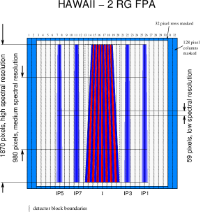
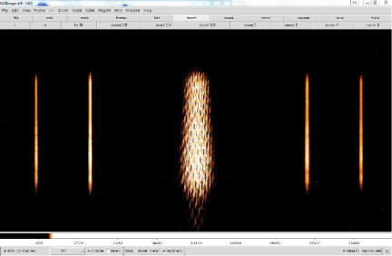
Figure 1: Expected (Left) vs. real data (Right) beams implementation on the MATISSE Hawaii detector (L-band). The wide central stripe contains the dispersed fringes (vertical spectral dispersion), while the 4 narrow stripes on the side contain the 4 single-telescope photometry used for flux calibration.

2 THE DATA REDUCTION SOFTWARE

The MATISSE DRS (called drsmat) aims at producing science-grade spectra, visibilities and phases out of the MATISSE raw datasets. The description of the main algorithms were described in details in several technical documents, and we report here the selected data reduction strategy and algorithms that were implemented in drsmat.

It is implemented in ANSI C and is fully integrated into the ESO pipeline software (i.e. it is interfaced with EsoRex[3] and Reflex[4]). The implementation uses the ESO-developped Common Pipeline Library (CPL)[5], the FITS format for intermediate frames, and the OIFITS format[6, 7] for the final data products (the MATISSE DRS will fully support the OIFITS version 2 format). The Reflex interfaces are made with xml files and also Organisation, Classification, and Association rules (OCA rules), and the GUI part is coded in python. The consortium actively supports ESO in the integration of drsmat in a Reflex workflow that will be used both at ESO and at the consortium sides for the reduction of the MATISSE data.

2.1 Overview

The basic input data are the raw frames of the MATISSE instrument, stored as FITS files. Let be $i^{\rm raw}(X,Y,t)$ this raw data intensity at time $t$, given at the $(X,Y)$ pixel detector index. Compared to the interferogram $i(x,\lambda,t)$, the raw data is affected by the following effects:

• Detector bias,

• Detector bad pixels,

• Detector + instrument flat field, plus eventually non-linear effects,

• Instrument distortion map, including a non-linear spectral dispersion law,

All these effects must be removed from the data in order to get the interferogram of eq. 1, out of which we extract the MATISSE observables. In addition, a calibration process leads to science-grade data. To do so, the software is organized into a data reduction cascade (shown in Fig. 2) that enables one to produce the calibration maps (mat_cal_det, mat_est_flat, mat_est_shift, mat_est_kappa), reduce the raw data into oifits files (mat_raw_estimates), calibrate the data (mat_cal_oifits), and then reconstruct an image out of the reduced data (mat_cal_imarec).

The very first step is to estimate the calibration maps like flat field map, bad pixels map, or distortion map out of calibration frames obtained during daytime using the internal calibration source of the instrument. They are used to correct the basic cosmetic of the detector and some optical effects of the instrument.

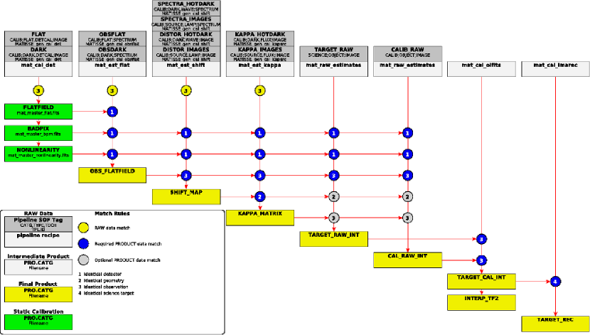
Figure 2: The MATISSE drsmat pipeline cascade, showing all the steps and files necessary to obtain a final science-grade dataset (calibrated oifits and/or reconstructed images).

2.2 Detector-specific cosmetics

2.2.1 Bad Pixels, Flat Field

The bad pixel map is derived from a series of cold dark raw frames obtained by increasing the integration time (DIT) from the MINDIT to five times the MINDIT with a minimum of 50 frames per exposure:

• First, spurious cosmics are detected by analyzing the intensity values of each pixel,

• Then, a robust median, a mean, and a standard deviation are computed for each pixel.

• For quality control purposes, the median, mean, and standard deviation of each pixel median of each series are calculated.

• For each pixel, a straight line is fitted to the 5 different median values. This fit results in an offset (pixel bias), a slope (dark current), and a fit quality.

• A pixel is marked as a bad pixel if the fit quality or the slope exceeds a certain limit (N sigmas of the standard deviation of the fit quality or slope for all detector pixels).

The flatfield map is derived from a series of illuminated frames ranging from detector noise up to detector saturation:

• First, the median of the matching series of cold dark frames is subtracted.

• Each frame is processed like the series of cold dark frames, i.e., mean, median, and RMS are computed.

• After normalization, the slopes of the straight lines from the flatfield images are used to compute the master gain map. However, in order to get a “detector” flatfield, the non-flat illumination must be taken into account. Therefore, the implemented algorithm must be adapted to the instrument optics.

The non-linearity map and the flat field are derived by fitting higher-order polynomials to the exposed frames, and saved as maps into fits files. We differentiate two types of flat fields in MATISSE: the detector flat field, which is obtained by a special device put into the beam, which diffuses the light onto the detector in a roughly uniform way, and the observing flat field, which is obtained through the spectrograph with a white lamp or a star without spectral features. The first one enables us to correct for detector pixel-to-pixel gain variations, while the second one allows us to correct for optics transmission variations.

2.2.2 Excess low frequency noise

During the Aquarius detector tests, and thanks to the ESO experience with VISIR, a strong temporal noise was effectively detected in the data. A set of exposures with increasing DIT was taken. This so called Excess Low Frequency Noise (ELFN) showed up in the temporal power spectra, as presented in Fig. 3. Pure white noise would result in a nearly flat temporal power spectrum. The increase at lower frequencies shows the ELFN.

Further investigations have lead to the following: the Aquarius ELFN is not a simple 1/f noise, the origin of the ELFN seems to be inside the semiconductor diode (pixel), the ELFN of different pixels is not correlated, the ELFN could not be reduced by using different readout modes, different multiplexer clocking schemes and delays or different bias voltages, the ELFN is proportional to the detector output signal level, ELFN cannot be seen in dark images, therefore CDS does not help, and finally ELFN was found on other MIR detectors (Si:As, InSb, etc.).

We expect this effect to be negligible for the coherent flux estimate (eq. 11), but likely present in the photometric estimates of MATISSE (eq. 7). The mitigation of this effect will need a fast chopping frequency like in VISIR, whose speed need to be addressed on sky.

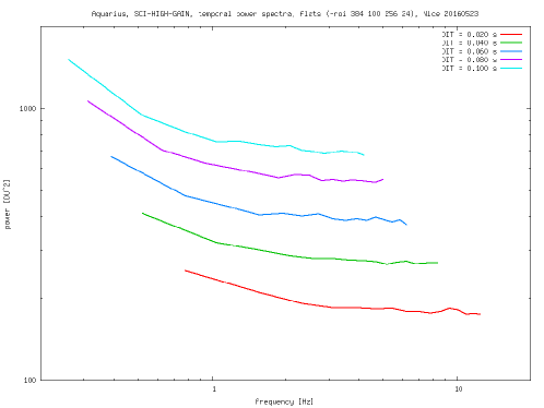
Figure 3: Average temporal power spectrum at several exposure times and increasing illumination. The ELFN shows up at frequencies lower than 1 Hz.

2.3 Optics calibration

2.3.1 Camera & spectrograph image distortion

Once the bad pixel map and flat field map have been produced, one can continue the instrument calibration with the determination of the image distortion. Since MATISSE contains a long-slit spectrograph, the distortion in the wavelength direction translates into a spectral dispersion law which is non-linear. We chose to treat the problem globally by computing a “shift map”.

The shift map is derived from a series of frames containing either a spatial grid (3 separate holes in the slit direction) or a spectral grid introduced by carefully-chosen plastic foils (for the wavelength direction), as shown in Fig. 4. This distortion estimate will be done at the same frequency as the flat field map or bad pixel map estimates.

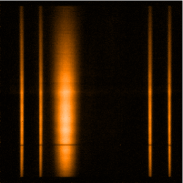
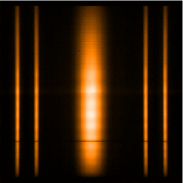
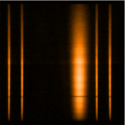
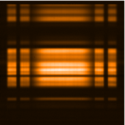
Figure 4: Three panels on the left: Spatial grid, made with three pinholes at different positions. Note that the photometric beams position is inverted compared to the interferometric beam one. Right: Spectral grid, made with plastic foils with spectral features. These snapshots were recorded in the N-band.

The distortion can be expressed as the relation between the pixel coordinates (X, Y) and the spectrograph coordinates $(x,\lambda)$ on the detector:

$$X = a(x,\lambda)x+b(x,\lambda)\lambda$$

$$Y = c(x,\lambda)x+d(x,\lambda)\lambda$$ (2)

$(X,Y)$ are the pixel indices, and $(x,\lambda)$ are the position and spectral dispersion, respectively. This can be written as a matrix relation:

$$\left(\begin{array}[]{cc}X\\ Y\end{array}\right)=\left(\begin{array}[]{cc}a(x,\lambda)&b(x,\lambda)\\ c(x,\lambda)&d(x,\lambda)\end{array}\right)\left(\begin{array}[]{cc}x\\ \lambda\end{array}\right)=\left(A\right)(x,\lambda)\left(\begin{array}[]{cc}x\\ \lambda\end{array}\right)$$ (3)

What we need then is to invert the matrix $(A)(x,\lambda)=\left(\begin{array}[]{cc}a(x,\lambda)&b(x,\lambda)\\ c(x,\lambda)&d(x,\lambda)\end{array}\right)$ to get the distortion relation:

$$\left(\begin{array}[]{cc}x\\ \lambda\end{array}\right)=(A)^{-1}(X,Y)\left(\begin{array}[]{cc}X\\ Y\end{array}\right)$$ (4)

Spatial Direction:

The spatial grid is first used. The $a$ parameter is estimated by fitting a polynomial to the position of the different features detected on the beams (3 features per beam):

$$a(x,\lambda)=a_{0}(\lambda)+a_{1}(\lambda)\times x+a_{2}(\lambda)\times x^{2}+...$$ (5)

Spectral direction:

We are then only interested in determining the $\lambda$-dependent distortion. Therefore, a “normal” $\lambda$-calibration frame (i.e. with the set of absorption plastic foils, or using sky absorption lines) should be available for that. In that case, one can determine the $d$ coefficient:

$$d(x,\lambda)=d_{0}(x)+a_{1}(x)\times\lambda+d_{2}(x)\times\lambda^{2}+...$$ (6)

We note here that this first step will give a coarse wavelength-calibration, which will be refined in a further step using telluric lines.

2.3.2 Shift and zoom, $\kappa$-matrix

As shown in Fig. 1 and Fig. 4, the MATISSE photometric beams have a different width than the interferometric beam, for obvious pixels-saving reasons. Therefore, since the spatial filtering is not perfect (due to the fact that we use pinholes instead of fibers, for technology readiness reasons), one needs to scale the photometric beams to the interferometric beam size by shifting and zooming them to the right place and scale.

In addition, one has to get the flux ratio coefficient between the flux measured in the interferometric beam and the one measured in the photometric beam, in order to have all the photometric information available to compute the observables.

The Shift and Zoom coefficients, together with the $\kappa$-matrix are computed using 4 illuminated frames, one for each of the telescope beams, the other beams being closed by shutters (see Fig. 5). The source is preferably artificial, part of MATISSE instrument, or could be a bright unresolved astronomical target as well.

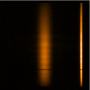
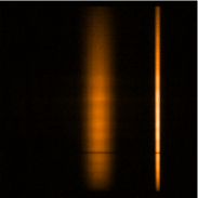
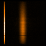
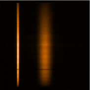
Figure 5: Kappa matrix acquisition sequence in the N-band, with alternatively just one out of four open shutter.

The photometric contribution $P^{\prime}_{i}(x,\lambda)$ of the telescope $i$ to the interferometric beam can be expressed as following:

$$P^{\prime}_{i}(x,\lambda,t)=\kappa_{ij}[x^{\prime},\lambda,s_{j}(\lambda),z_{j}(\lambda)]\times P_{ij}(x^{\prime},\lambda,t)$$ (7)

where $P_{ij}(x^{\prime},\lambda,t)$ is a vector containing the contribution of the telescope $i$ to the photometric beams $j$ (after chopping correction, see section 2.4.1), $\kappa_{ij}$ is the linear transformation matrix of the intensities in the photometric channels into the interferometric channel (the so-called ”$\kappa$-matrix”), and $s_{j}(\lambda)$, $z_{j}(\lambda)$ are the shift offset and zoom coefficient to match the photometric beam $j$ into the interferometric beam.

We determine therefore the $\kappa$-matrix and the shift-and-zoom coefficients by fitting the photometric beam shape and intensity to the interferometric beam for each selected wavelength.

2.3.3 Applying cosmetics

The first steps of the data reduction are:

1. Subtracting the average (cold) dark ${\rm DARK}(X,Y)$ in each frame,

2. Compensating of the space-variant gain in each frame by division of each frame through the ${\rm FFM}(X,Y)$ (flat-field map),

3. Interpolating detector bad pixels in each frame with the ${\rm BPM}(X,Y)$ (bad pixel map),

4. Applying the distortion matrix to transform $(X,Y)$ to $(x,\lambda)$, the coordinates of the data,

5. Adjusting the photometric contribution in the interferometric beam by applying the $\kappa$-matrix, shift, and zoom coefficients

The result of treating the three first effects is shown in Fig. 6. The two last corrections are being tested right now on the mounted instrument in the Nice laboratory.

The results of these processes are: a cleaned-up fringe pattern $i^{{}^{\prime}}(x,\lambda,t)$, and cleaned-up photometric estimates $P^{{}^{\prime}}_{i}(x,\lambda,t)$.

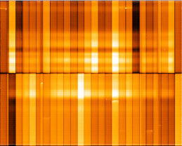
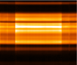
Figure 6: Left: The raw image from the Aquarius detector (7-13 $\mu$m) contains four photometric channels, the interferometric channel and 16 reference areas, showing bad pixels and detector channel offsets. Right: The same image after the calibration step contains the photometric channels and the interferometric channel only.

2.4 How to tackle the multiple-stage modulations in MATISSE

As described in Petrov et al. (2016)[8], MATISSE includes a three-stage modulation process for the mitigation of the sky background (as MATISSE works in the mid-infrared). These stages are namely chopping, spatial modulation and temporal modulation, in addition to beam commutation, which is used to clean up the phases out of the instrumental effects.

2.4.1 Chopping

Chopping produces alternatively science and sky frames with a switching frequency as fast as 1Hz. The first step is to remove these sky frames to the science frames, resulting in removing the bulk of the background contribution ($\approx 99$%):

$$i(x,\lambda,t)=i^{\rm\,obj}(x,\lambda,t)-i^{\rm\,sky}(x,\lambda,t)$$ (8)

2.4.2 Spatial modulation

Spatial modulation separates, in the Fourier plane, the fringes energy (“fringe peak”) from the flux energy (“photometric peak”). Therefore, a simple Fourier processing along the $x$ axis will cancel further out the contribution of the background to the data. Correlated fluxes are computed just by Fourier-Transforming the clean interferogram:

$$I^{{}^{\prime}}(u,\lambda,t) = {\rm FT}_{x}[i(x,\lambda,t)]$$ (9)

$$= F_{00}(u,\lambda,t)+\sum_{i=1}^{4}\sum_{j=i+1}^{4}\left[F_{ij}(u-f_{ij},\lambda,t)\cdot V_{ij}(\lambda)\cdot e^{\i\Phi_{ij}(\lambda,t)}\right]$$

where $u$ is a spatial frequency, $f_{ij}$ is the fringe rate, as explained below eq. 1, $V_{ij}(\lambda)$ is the target visibility, $\Phi_{ij}(\lambda,t)$ is the phase of the target plus piston, and $F_{ij}(u,\lambda,t)$ is a function of the photometric contributions $P^{\prime}_{i}(x,\lambda)$, involving Fourier Transforms and correlations, representing the shape of the peaks. We note that $\sum\limits_{u}F_{ij}(u,\lambda,t)=\sqrt{\sum\limits_{x}P_{i}(x,\lambda,t)\cdot P_{j}(x,\lambda,t)}$, and that $F_{00}(u,\lambda,t)$ represents the photometry peak.

The background residuals left after chopping contribute only to $F_{00}(u,\lambda,t)$ at first order, as the background does not contain any coherent information. At the frequency of each fringe peak $f_{ij}=b_{ij}/\lambda$, we have:

$$I^{{}^{\prime}}_{ij}(\lambda,t)=I^{{}^{\prime}}(f_{ij},\lambda,t)=F_{ij}(0,\lambda,t)\cdot V_{ij}(\lambda)\cdot e^{\i\Phi_{ij}(\lambda,t)}+B^{\rm res}_{ij}(\lambda,t)$$ (10)

where the contribution of the residual background $B^{\rm res}_{ij}(\lambda,t)=F_{0}(f_{ij},\lambda,t)$ is much smaller than at the frequency 0 (as seen in Fig. 7 on top and bottom row).

2.4.3 Temporal modulation

In addition to the spatial modulation, a temporal modulation is introduced by piezoelectric actuators, changing the optical path difference (OPD) $\Delta^{\rm mod}_{ij}(t)$ by a fraction of the wavelength between consecutive frames. Let us consider that there are $N_{T}$ steps over an OPD range of $\Delta_{ij}$ during one modulation cycle $T$. The modulation is then $\Delta^{\rm mod}_{ij}(t)=\frac{k}{N_{T}}\Delta_{ij}$, $k$ being the modulation step number.

On needs to consider the fringes “freezed” over the modulation time $T$ in order to consider $\Delta^{\rm atm}_{ij}(t)$ constant. Therefore, the modulation cycle must be done over one atmosphere coherence time $T\approx\tau_{0}$, or in conjunction with a fringe tracker which freezes the fringes over a time $T\approx\tau_{\rm FT}$.

A de-modulation is applied to the previous Fourier-Transform, baseline-by-baseline, and we integrate the fringe peak $I^{{}^{\prime}}_{ij}(\lambda,t)$ over one modulation cycle (the $N_{T}$ steps of modulation). We do so by multiplying it with a phasor containing the counter-modulation:

$$I^{{}^{\prime\prime}}_{ij}(\lambda,T) = \frac{1}{N_{T}}\sum_{k=0}^{N_{T}}I^{{}^{\prime}}_{ij}(\lambda,t)\times e^{-2i\pi\Delta^{\rm mod}_{ij}(t)/\lambda}$$ (11)

$$= F_{ij}(0,\lambda,t)\cdot V_{ij}(\lambda)\cdot e^{i\Phi_{ij}(\lambda,t)}+\delta B^{\rm res}_{ij}(\lambda,t)$$

The background residual is further reduced by the modulation, leading to the final residual background $\delta B^{\rm res}_{ij}(\lambda,t)$:

$$\delta B^{\rm res}_{ij}(\lambda,t)=B^{\rm res}_{ij}(\lambda,t)\times\frac{1}{N_{T}}\sum_{k=0}^{N_{T}}e^{\left[-2i\pi k\cdot\Delta_{ij}/(N_{T}\cdot\lambda)\right]}$$ (12)

The effect of demodulation can be seen in Fig. 7, middle row. The combination of spatial modulation, temporal modulation and chopping are the three ways selected in MATISSE to tackle the dominance of the background. Please note that neither the spatial nor the temporal modulation can be applied to the photometries. Therefore, the rejection of the sky background in the photometric estimates rely only on Chopping, and will be of much lower quality.

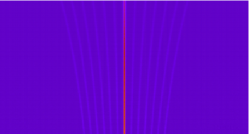
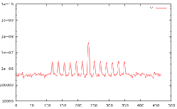
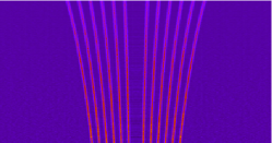
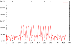
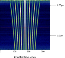
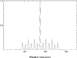
Figure 7: Left column: Fourier transform of the MATISSE fringe pattern. Right column: cut at one wavelength. Top: Simulated fringe pattern after the chopping correction. Middle: Same as before, but after the temporal demodulation applied. Bottom: Same as first one but on the real first fringes data shown in Fig. 1. The (de)modulation is not yet operational on the instrument.

2.5 Estimators

Once the complex coherent flux $I^{{}^{\prime\prime}}_{ij}(\lambda,T)$ has been computed, it is possible to compute the estimators, i.e. the raw visibilities and phases of the object. These estimators are split between incoherent estimators (speckle-like), that can be computed without the knowledge of the optical path difference, and coherent estimators that need an appropriate atmospheric OPD estimate, be it simply due to the turbulence or to higher-order effects (longitudinal dispersion).

2.5.1 “Incoherent” estimators

Squared visibility

Squared visibilities are computed as follows:

$$V_{ij}^{2}(\lambda)=\frac{\sum\limits_{u}\left<|I^{{}^{\prime}}(u,\lambda,t)|^{2}-\beta\right>_{t}}{2\cdot\sum\limits_{x}\left<\overline{P_{a}}^{\prime}(x,\lambda,t)\cdot\overline{P_{b}}^{\prime}(x,\lambda,t)\right>_{t}}$$ (13)

where $u$ is the frequency around the considered baseline, and $\beta$ a bias estimated on $I^{{}^{\prime}}$ outside the range of frequencies where the fringe peaks are present, and $\overline{P_{a}}^{\prime}(x,\lambda,t)$ and $\overline{P_{b}}^{\prime}(x,\lambda,t)$ are the estimates of the photometric fluxes transformed into the interferometric channel (see eq. 7).

In the case where there are no photometries recorded (like in HIGH-SENS mode without a photometric acquisition sequence), the squared visibilities are simply not computed. Instead, the user should use the correlated fluxes, i.e. the upper part of eq. 13:

$${\rm CF}_{ij}^{2}(\lambda)=\sum\limits_{u}\left<|I^{{}^{\prime}}(u,\lambda,t)|^{2}-\beta\right>_{t}$$ (14)

Closure Phase

The bispectrum is calculated by:

$$O^{(3)}_{ij}(\lambda)=\left<I^{{}^{\prime}}(u,\lambda,t)\times I^{{}^{\prime}}(v,\lambda,t)\times{I^{{}^{\prime}}}^{*}(u+v,\lambda,t)\right>_{t}$$ (15)

where $u$, $v$, and $u+v$ are the frequencies of the baselines involved in the closure relation. An example MATISSE bispectrum can be seen in Fig. 8. Out of the 5 peaks that can be seen, just 4 contain useful information from the 4 closure phases available at 4 telescopes (the middle-left peak is a spurious peak coming from the contamination of the central photometric peak).

This average bispectrum contains an additive noise bias terms plus a multiplicative one, because of the all-in-one combination of the interferograms. These biases need to be subtracted in order to get closure phases without systematic errors, following specific recipes[9, 10].

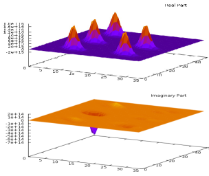
Figure 8: Example bispectrum values computed on simulated MATISSE data. Top graph: real part, and bottom graph: imaginary part. The middle-left peak is spurious.

2.5.2 “Coherent” estimators

Coherent estimators need an appropriate OPD estimate. We describe here briefly what we envision to include in drsmat. The complex coherent flux is provided by the equation 11.

The phase term $\Phi_{ij}(\lambda,t)$ depends on the variations of the atmospheric properties (temperature, pressure), producing an achromatic variation of OPD (but not phase), and it depends also on the refractive index $n(\lambda))$ of air, which is chromatic and dependent of its water vapor composition. It can be expressed as:

$$\Phi_{ij}(\lambda,t)=\Phi_{ij}^{\rm obj}(\lambda)+2\pi\frac{\Delta_{ij}^{\rm atm}(t)}{\lambda}+2\pi\frac{\Delta_{ij}^{\rm atm}(t)}{\lambda}\cdot[n(\lambda,t)-1]$$ (16)

the different terms are the following:

• $\Delta_{ij}^{\rm atm}(t)$: achromatic part of the atmospheric OPD,

• $[n(\lambda,t)-1]\approx a(\lambda)+b(t)$, chromatic term with $a(\lambda)$ wavelength-dependent but roughly static [11, 12], and $b(t)$ wavelength independent, but with strong variations in time [13]

• $\Phi_{ij}^{\rm obj}(\lambda)=\Phi_{ij}^{(0)}+\Phi_{ij}^{(1)}/\lambda+\Phi_{ij}^{\rm diff}(\lambda)$: the object phase, which can be decomposed in a Taylor series containing the differential phase $\Phi_{ij}^{\rm diff}(\lambda)$.

Achromatic Optical Path Difference estimates:

MATISSE will compute the achromatic OPD using a VEGA-like algorithm[14, 15]: a 2D-Fourier Transform (FT) is computed, to take profit of the multi-axial beam combination of MATISSE. The fringe peak in the power spectrum appears as an offset peak, whose offset is proportional to the OPD. The great advantage of this method is that the peak is concentrated onto a small location of the 2D map, whereas the noise is spread everywhere, hence contributing to a smaller fraction of the peak noise. In addition, there is no ambiguity at OPD 0, contrary to a MIDI-like estimate.

This 2D-FT can be computed in two steps, first in the spatial direction and second in the spectral direction, allowing us to counteract the OPD modulation pattern before elevating the Fourier Transform to its square, and hence increasing tremendously the SNR of the peak detection. This is also the way the fringe pattern will be detected in real time with the instrument.

Another option implemented for OPD determination is a fit to the complex coherent flux phase, in the very same way as it is done for AMBER [16].

The computed atmospheric OPD contains then the two terms: ${\rm OPD}=\Delta_{ij}^{\rm atm}(t)+\Phi_{ij}^{(1)}$.

Chromatic OPD estimates:

ESO provides information through the ambient conditions monitor that will be sufficient to correct the data from the chromatic dry and wet air dispersion, down to accuracies of 3 degrees in K band and down to 10 degrees in N-band.

The static water vapor term $a(\lambda)$ will be computed using the pressure $P$, temperature $T$ (in the tunnels), and relative humidity of the ambient air $R_{h}$. We add to these the partial pressure of CO₂, which can be hard-coded to an average value at Paranal. The fraction of humidity is converted into partial pressure of water vapor $p_{wv}=R_{h}\times P$. The $\lambda$-dependent shape of the chromatic phase $a(\lambda)$ is then be determined based on computed optical index of air $n$ as a function of wavelength [11, 12]. The next step is to compute phases, and therefore we also use the information of the delay lines position to compute the difference of delay for each baseline: if $A_{i}$ is the static optical path introduced by the delay line $i$, and $OPL_{i}$ the dynamic path, $A_{i}+OPL_{i}$ is the total path of air introduced by each delay line. Per baseline $ij$, the path to use for the chromatic OPD is therefore $\delta_{ij}=A_{i}+OPL_{i}-A_{j}-OPL_{j}$. The chromatic phase is then computed by $\phi^{\rm chrom}(\lambda)=2\pi a(\lambda)\frac{\delta_{ij}}{\lambda}$, with $n$ the computed index of air, and $\lambda$ the wavelength of interest.

The water vapor phase offset, time-variable, $\Delta_{ij}^{\rm atm}(t)\cdot b(t)$, will be obtained by averaging the phase term in the wavelength-direction after subtraction of the atmospheric OPD. As a consequence, it also removes the object-related phase offset $\Phi_{ij}^{(0)}$. The result is therefore $\Delta_{ij}^{\rm atm}(t)\cdot b(t)+\Phi_{ij}^{(0)}$.

All these calculations yield $\Delta_{ij}^{\rm atm}(t)+\Phi_{ij}^{(1)}$, $a(\lambda)$, and $\Delta_{ij}^{\rm atm}(t)\cdot b(t)+\Phi_{ij}^{(0)}$.

Differential phase:

After that step, the computed phase is transformed into a differential phase the standard way [17, 18, 19]. We recall it briefly here. First, we multiply the Fourier transform of the correlated interferograms by the counter OPD phasor. This yields the OPD-free complex coherent flux:

$${\rm CF}_{ij}(\lambda,t) = I^{{}^{\prime\prime}}_{ij}(\lambda,t)\times e^{-2i\pi\,\left(\left[\Delta_{ij}^{\rm atm}(t)/\lambda+\Phi_{ij}^{(1)}\right]+\left[\Delta_{ij}^{\rm atm}(t)\cdot b(t)+\Phi_{ij}^{(0)}\right]+a(\lambda)\right)}$$ (17)

$$= F_{ij}(0,\lambda,t)\cdot V_{ij}(\lambda)\cdot e^{i\,\Phi_{ij}^{\rm diff}(\lambda)}$$

Averaging this OPD-free complex coherent flux over time yields the following products:

• $<F_{ij}(0,\lambda,t)>\cdot V_{ij}(\lambda)$ : correlated flux degraded by the not corrected beam overlap

• $\Phi_{ij}^{\rm diff}(\lambda)$ : differential phase, with any wavelength-linear phase term set to zero.

Coherent visibility:

Finally, it is possible to continue the processing to lead to a linear visibility estimate. For that, we divide the correlated flux by the photometric factor. This is the last optional step, yielding the linear visibility estimate:

$$V_{ij}(\lambda))=\left|\frac{\sum\limits_{u}\left<{\rm CF_{ij}(u,\lambda,t)}\right>_{t}}{\sqrt{\left<\sum\limits_{x}P_{i}(x,\lambda,t)\cdot P_{j}(x,\lambda,t)\right>_{t}}}\right|$$ (18)

In the case where there are no photometries recorded (like in HIGH-SENS mode), this term is not computed, as for the squared visibilities.

2.6 Data calibration

To calibrate the data, we apply the same recipes as in AMBER[20], i.e.:

• We start with searching calibrator stars diameters in published catalogs,

• we divide the calibrators visibilities by their expected visibilities and store the transfer function result in new files,

• we interpolate the transfer function to the time of the science observations with a Gaussian-weighted average (typical FWHM 1hr),

• we divide the science visibilities with the interpolated transfer function and store the result as calibrated science-grade data files.

drsmat uses the ESO-developed Reflex interface to run all the steps, and the calibration part contains a display of the result, allowing the user to select the relevant calibration stars (see Fig. 9)

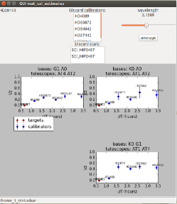
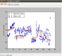
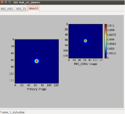
Figure 9: Example displays of the drsmat workflow: Left: Transfer function plot and selection, Middle: Visibility comparison plot between observed (blue) and reconstructed (red) visibilities, coming from the image reconstruction process, Right: Image display showing the reconstructed image and the prior image.

2.7 Image reconstruction

The last step of drsmat is the image reconstruction. MATISSE will use the IRBIS algorithm, which was specially developed for it. The content of IRBIS is extensively described in another paper of this conference[21]. The drsmat software displays the results of the reconstruction through a python interface, shown in Fig. 9.

3 CONCLUSION

We presented the MATISSE data reduction software drsmat as it has been implemented for the MATISSE instrument. drsmat produces calibrated dispersed visibilities, closure phases and differential phases from the beginning, and also includes the IRBIS algorithm for image reconstruction. MATISSE is presently undergoing laboratory tests to verify that it meets all the necessary requirements to reach its science goals. The tests of drsmat is a significant part of these tests.

- [1] Lopez, B., Lagarde, S., Jaffe, W., et al., “An Overview of the MATISSE Instrument / Science, Concept and Current Status,” The Messenger 157, 5 (2014).
- [2] Millour, F., Tatulli, E., Chelli, A. E., Duvert, G., Zins, G., Acke, B., and Malbet, F., “Data reduction for the AMBER instrument,” SPIE Conference Series 5491, 1222 (2004).
- [3] ESO CPL Development Team, “EsoRex: ESO Recipe Execution Tool.” Astrophysics Source Code Library (Apr. 2015).
- [4] Freudling, W., Romaniello, M., Bramich, D. M., Ballester, P., Forchi, V., García-Dabló, C. E., Moehler, S., and Neeser, M. J., “Automated data reduction workflows for astronomy. The ESO Reflex environment,” A&A 559, A96 (Nov. 2013).
- [5] McKay, D. J., Ballester, P., Banse, K., Izzo, C., Jung, Y., Kiesgen, M., Kornweibel, N., Lundin, L. K., Modigliani, A., Palsa, R. M., and Sabet, C., “The common pipeline library: standardizing pipeline processing,” in [Optimizing Scientific Return for Astronomy through Information Technologies ], Quinn, P. J. and Bridger, A., eds., Proc. SPIE 5493, 444–452 (Sept. 2004).
- [6] Pauls, T. A., Young, J. S., Cotton, W. D., and Monnier, J. D., “A Data Exchange Standard for Optical (Visible/IR) Interferometry,” PASP 117, 1255 (2005).
- [7] Duvert, G., Young, J., and Hummel, C., “OIFITS 2: the 2nd version of the Data Exchange Standard for Optical (Visible/IR) Interferometry,” ArXiv e-prints (Oct. 2015).
- [8] Petrov, R. et al., “A triple modulation to optimize the accuracy of the vlti instrument matisse,” in this conference: SPIE Conference Series (2016).
- [9] Wirnitzer, B., “Bispectral analysis at low light levels and astronomical speckle masking,” Journal of the Optical Society of America A 2, 14 (1985).
- [10] Gordon, J. A. and Buscher, D. F., “Detection noise bias and variance in the power spectrum and bispectrum in optical interferometry,” A&A 541, A46 (May 2012).
- [11] Ciddor, P. E., “Refractive index of air: new equations for the visible and near infrared,” Applied Optics 35, 1566 (1996).
- [12] Mathar, R. J., “Refractive index of humid air in the infrared: model fits,” Journal of optics 9, 470 (2007).
- [13] Jaffe, W. J., “Coherent fringe tracking and visibility estimation for MIDI,” SPIE Conference Series 5491, 715 (2004).
- [14] Mourard, D., Clausse, J. M., Marcotto, et al., “VEGA: Visible spEctroGraph and polArimeter for the CHARA array: principle and performance,” A&A 508, 1073–1083 (2009).
- [15] Mourard, D., Bério, P., Perraut, K., et al., “Spatio-spectral encoding of fringes in optical long-baseline interferometry. Example of the 3T and 4T recombining mode of VEGA/CHARA,” A&A 531, A110 (2011).
- [16] Tatulli, E., Millour, F., Chelli, A., et al., “Interferometric data reduction with AMBER/VLTI. Principle, estimators, and illustration,” A&A 464, 29–42 (2007).
- [17] Millour, F., Vannier, M., Petrov, R. G., Chesneau, O., Dessart, L., and Stee, P., “Differential Interferometry with the AMBER/VLTI instrument: Description, performances and illustration,” EAS Publications Series 22, 379–388 (2006).
- [18] Millour, F., “Circumstellar Matter Studied by Spectrally-Resolved Interferometry,” Astronomical Society of the Pacific Conference Series 464, 15 (2012).
- [19] Millour, F., “Interferometry concepts,” EAS Publications Series 69, 17–52 (2014).
- [20] Millour, F., Valat, B., Petrov, R. G., and Vannier, M., “”Advanced” data reduction for the AMBER instrument,” SPIE Conference Series 7013 (2008).
- [21] Hofmann et al., “Image reconstruction method irbis for optical/infrared long-baseline interferometry,” in this conference: SPIE Conference Series (2016).