Bifurcation equations for periodic orbits of implicit discrete dynamical systems

Abstract.

Bifurcation equations, non-degeneracy and transversality conditions are obtained for the fold, transcritical, pitchfork and flip bifurcations for periodic points of one dimensional implicitly defined discrete dynamical systems. The backward Euler method and the trapezoid method for numeric solutions of ordinary differential equations fall in the category of implicit dynamical systems. Examples of bifurcations are given for some implicit dynamical systems including bifurcations for the backward Euler method when the step size is changed.

1. Introduction

1.1. Motivation

In this paper we study bifurcation equations and transversality conditions for local bifurcations of $p$-periodic points in one-dimensional discrete dynamical systems defined implicitly, with $p$ a positive integer. In particular, we focus our attention on the fold, transcritical, pitchfork and flip, i.e., the most frequently found in applications. The main result of the paper is to obtain expressions for the general bifurcation equations and transversality conditions in dynamical systems defined implicitly.

Implicitly defined discrete and continuous dynamical systems are not very well studied, only very recently Albert Luo published “the first monograph to discuss the implicit mapping dynamics of periodic flows to chaos” [20]. The singularities of some implicit continuous dynamical systems in dimension two have been addressed in [6], namely the Clairaut system. Nevertheless, it is an interesting and open field of research. This type of dynamical system appears in applications, namely in the theory of PDE in the works of Sharkovsky and co-workers [4, 19, 26, 27, 28], in Mathematical Economics directly [22] or in the context of backward dynamics [14, 21]. It appears also in the context of Control Theory [13]. These implicit dynamical systems appear also in numerical methods for ordinary differential equations, v.g., the backward Euler, the trapezoid method [29, 12] and the Runge-Kutta implicit method, see the recent article [30]. Implicit numeric methods are very useful when the original equations exhibit stiffness, see for instance [10, 11]. In [18] the implicit Euler method was used in a concrete mechanical problem. Some implicit iterative schemes were transformed in forward dynamical systems using numerical methods, v.g., Newton method, [7]. In implicit numerical schemes it is possible to prove the existence of period doubling when the step size parameter increases as we do with a simple example at the end of this article. It is also interesting to see the existence of chaos when the parameter $h$ is big enough, but still relatively small.

The case of $p$-periodic points with $p>1$, is very intricate, the computations increase its complexity extraordinary with the powers of the normal form, as we can see in this paper in the case of the pitchfork. For that reason, we study codimension $1$ cases, the most common in applications.

The study of one-dimensional bifurcations makes sense, since many higher order systems can be reduced [25] to lower order dimensional dynamics via center manifold and Poincaré map techniques as in [15], using spectral properties and quasi-periodicity [23], and in periodic non-autonomous systems using Floquet theory [5].

It is completely open and would be interesting to investigate the invariance of the bifurcation equations for periodic non-autonomous systems defined implicitly in the line of work of [24].

One of the main reasons of this paper is to provide computational tools for the applied researcher dealing with implicitly defined dynamical systems. It is possible to study the bifurcations that can occur without the knowledge of an explicit difference equation. All the formulae are programmable using the usual platforms available for mathematicians. The examples where prepared using Wolfram Mathematica 10.0.

We follow the terminology of [17].

1.2. Overview

We organized this paper in four sections. In Section 2 we introduce basic concepts.

In Section 3, the core of this work, we study in detail the equations of bifurcation for $p$-periodic orbits of implicitly defined dynamical systems.

In Section 4 we present examples, namely on the Euler method for numerical solutions of ordinary differential equations. In the implicit difference equations of numerical methods we show the existence of bifurcation depending on the step size parameter $h$, and the existence of chaos even in very simple examples.

2. Preliminaries

2.1. Basic definitions and notation

We define implicitly a discrete dynamical system using instead of the classic definition

(1) $$x_{n+1}=f(x_{n})\text{, }x_{n}\in I\text{, with }n\in\mathbb{\mathbb{N}}\text{,}$$

the alternative one

$$F\left(x_{n},x_{n+1}\right)=0\text{, for }x_{n},x_{+1}\in I\text{, with }n\in\mathbb{\mathbb{N}}\text{,}$$

where $I$ is a real interval (not necessarily compact and maybe $\mathbb{R}$), where we input $x_{n}$ and solve for $x_{n+1}$ giving an initial condition $x_{0}\in I$. The usual Euclidean distance is defined in $I$. The map $F$ is sufficiently differentiable for the purposes of bifurcation theory, assumption that we keep in this paper. We suppose that given $F\left(x,y\right)=0$, there exists the solution $\left(x_{0},y_{0}\right)$, and an implicit function $y=f\left(x\right)$ with $y_{0}=f\left(x_{0}\right)$ such that

$$F\left(x,f\left(x\right)\right)=0\text{, }$$

in a suitable neighborhood of $\left(x_{0},y_{0}\right)$. We follow [16] concerning the implicit function theorem. For the purposes of this article we admit the existence of the necessary solutions in the appropriate neighborhoods of the bifurcation points. Obviously, each particular dynamical system defined implicitly must be studied to ensure the existence of the iteration function $f\left(x\right)$.

In the sequel, by ${\mathcal{C}}\left(D\right)$ we denote the collection of all continuous maps in its domain $D$, by ${\mathcal{C}}^{1}\left(D\right)$ the collection of all continuously differentiable elements of ${\mathcal{C}}\left(D\right)$ and, in general by ${\mathcal{C}}^{s}\left(D\right),$ $s\geq 1,$ the collection of all elements of ${\mathcal{C}}\left(D\right)$ having continuous derivatives up to order $s$ in $D.$

The $p$ composition of $f$ a real function of real variable is denoted by $f^{p}$, the usual power is denoted by $\left(f\right)^{p}$.

Let $f\in{\mathcal{C}}^{1}\left(D\right)$, and let $x_{0}$ be a periodic point of period $p$, $x_{0}$ is called a hyperbolic attractor if $|\frac{df^{p}(x_{0})}{dx}|<1$, a hyperbolic repeller if $|\frac{df^{p}(x_{0})}{dx}|>1$, and non-hyperbolic if $|\frac{df^{p}(x_{0})}{dx}|=1$.

Definition 2.1.

We say that two continuous maps $f:I\rightarrow I$ and $g:J\rightarrow J$, are topologically conjugate, if there exists a homeomorphism $h:I\rightarrow J$, such that $h\circ f=g\circ h$. We call $h$ the topological conjugacy of $f$ and $g$.

We use $\alpha$ for a real parameter.

Definition 2.2.

If $f\left(\cdot,\alpha\right)$ is a family of maps, then the regular values $\alpha$ of the parameters are those which have the property that $f\left(\cdot,\widetilde{\alpha}\right)$ is topologically conjugate to $f\left(\cdot,\alpha\right)$ for all $\widetilde{\alpha}$ in some open neighbourhood of $\alpha$. If $\alpha$ is not a regular value, it is a bifurcation value. The collection of all the bifurcation values is the bifurcation set, $\Omega\subset\mathbb{R}$, in the parameter space.

Let $f\left(\cdot,\alpha_{0}\right)$ be a parameter dependent family of maps in ${\mathcal{C}}^{s}\left(D\right)$. Let $\alpha_{0}$ be a particular parameter and $a\in D$ be a fixed point of the $p$ composition map $f\left(\cdot,\alpha_{0}\right)$, with $p$ a minimal positive integer, i.e.,

$$a=f^{p}\left(a,\alpha_{0}\right)\text{,}$$

$a$ is a periodic point of the dynamical system. The condition of $a$ being non-hyperbolic is necessary for the existence of a local bifurcation. The existence and nature of that bifurcation depends on other symmetry and differentiable conditions that we will see bellow. If there exists a local bifurcation we say that $(a,\alpha_{0})$ is a bifurcation point (when there is no risk of confusion, we say that $a$ is a bifurcation point).

Notation 2.3.

For notational simplicity we consider the real parameter $\alpha$ as a standard variable along with the dynamic variable $x$, i.e., we write $F\left(x,y,\alpha\right)$ instead of $F_{\alpha}\left(x,y\right)$, reserving the last slot for the parameter, keeping in mind that the compositions are always in the dynamic variables $x$ and $y$. In this paper we never use $f_{\alpha}$ to mean dependence on the parameter.

When there is no danger of confusion and no operations regarding the parameter, we denote the evaluation of functions depending on the dynamic variable and the parameter omitting the later, for instance $F\left(x,y,\alpha\right)$ or $f\left(x,\alpha\right)$ will be denoted by $F\left(x,y\right)$ or $f\left(x\right)$ in order to avoid to overload the complicated notation needed for the computations of chain rules. Nevertheless, all the maps in this paper depend on the parameter as well on the dynamic variable. We deal with parameter depending families of maps, even when that dependence is not visible in some formulas or expressions.

We denote the derivatives relative to some variable $y$ by $\partial_{y}$. Repeated differentiation relative to the same variable is denoted by $\partial_{y^{n}}$, for instance $\partial_{yyy}=\partial_{y^{3}}$. When there is no danger of confusion, we denote strict partial derivatives, i.e., not seeing composed functions, by a subscript. For instance, the third partial derivative of $f$ relative to $y$ is, in that case, denoted by $f_{yyy}$ or $f_{y^{3}}$.

This means, in particular, that when dealing with the composition of real scalar functions $F\left(x,y\right)$ with $g\left(x,y\right)$ and $h\left(x,y\right)$, we have the usual chain rule

$$\partial_{x}F\left(g\left(x,t\right),h\left(x,t\right),\alpha\right)=\\ F_{x}\left(g\left(x,t\right),h\left(x,t\right),\alpha\right)g_{x}\left(x,t\right)+F_{y}\left(g\left(x,t\right),h\left(x,t\right),\alpha\right)h_{x}\left(x,t\right)\text{,}$$

2.2. Classic conditions for fold, transcritical, pitchfork and flip bifurcations

In this paragraph, we recall briefly the conditions of codimension $1$ local bifurcations with derivatives $\partial_{x}f^{p}(x_{0})=\pm 1$.

We first consider the case $\partial_{x}f^{p}(x_{0})=+1$. Giving a discrete dynamical system generated by the iteration of $f$ in its domain $D$, and a real parameter $\alpha$, in order to compute the bifurcation points one has to solve the bifurcation equations [17]

(2) $$\begin{array}[c]{l}{f}^{p}(x,\alpha)=x\text{, fixed point equation}\\ {f}_{x}^{p}(x,\alpha)=1\text{, non-hyperbolicity condition.}\end{array}$$

2.2.1. Fold

The simplest of such local bifurcations is the fold or saddle node bifurcation. One assumes, in this case, the non-degeneracy condition

(3) $${f_{x^{2}}}(x,\alpha)\not=0$$

and the transversality condition [17]

(4) $$f_{\alpha}\left(x,\alpha\right)\not=0.$$

We set generically that $\alpha\in\mathbb{R}$, since one needs only one parameter to unfold locally this singularity [1, 2, 3, 8, 9, 17]. The normalized germ of this bifurcation is

$$x\pm x^{2}\text{,}$$

with principal family

$$x\pm x^{2}+\alpha\text{,}$$

which is locally weak topologically conjugated to any other family [2, 17] satisfying the bifurcation conditions.

2.2.2. Transcritical

Another simple bifurcation is the transcritical, in this case is a bifurcation with symmetry. One assumes, in this case, the non-degeneracy condition

(5) $${f_{x^{2}}}(x,\alpha)\not=0,$$

the transversality condition of the fold fails

(6) $$f_{\alpha}\left(x,\alpha\right)=0,$$

becoming a new degeneracy condition. The symmetry condition states that the fixed point of $f$ persists. Without loss of generality we consider that $0$ is that fixed point. The new transversality condition is

$$f_{x\alpha}\left(x,\alpha\right)\not=0\text{.}$$

Again, we set generically that $\alpha\in\mathbb{R}$, since one needs only one parameter to unfold locally this singularity [1, 2, 3, 8, 9]. The principal family is now

$$\left(1+\alpha\right)x\pm x^{2}\text{,}$$

which is weak topologically conjugated to any other family [2, 17] satisfying the bifurcation conditions.

2.2.3. Pitchfork

The last type of bifurcation we consider with derivative $\partial_{x}f^{p}(x_{0})=+1$ is the pitchfork, another bifurcation with the same symmetry on the fixed point as the transcritical. One assumes, in this case, the extra degeneracy condition

$${f_{x^{2}}}(x,\alpha)=0,$$

and the new non-degeneracy condition

(7) $${f_{x^{3}}}(x,\alpha)\not=0.$$

The transversality condition of the fold fails again

(8) $$f_{\alpha}\left(x,\alpha\right)=0\text{,}$$

and the transversality condition is assumed again to be

$$f_{x\alpha}\left(x,\alpha\right)\not=0\text{.}$$

We set generically that $\alpha\in\mathbb{R}$ [1, 2, 3, 8, 9]. The principal family is now

$$\left(1+\alpha\right)x\pm x^{3}\text{,}$$

which is weak topologically conjugated to any other family [2, 17] satisfying the bifurcation conditions.

2.2.4. Flip

We consider now the conditions of codimension $1$ local bifurcations with derivative $\partial_{x}f^{p}(x_{0})=-1$.

One has to solve the bifurcation equations [17]

(9) $$\begin{array}[c]{l}{f}^{p}(x,\alpha)=x\text{, fixed point equation}\\ {f}_{x}^{p}(x,\alpha)=-1\text{, non-hyperbolicity condition.}\end{array}$$

One assumes, in this case, the generic non-degeneracy condition

(10) $$\frac{1}{2}\left(f_{x^{2}}\left(x,\alpha\right)\right)^{2}+\frac{1}{3}f_{x^{3}}\left(x,\alpha\right)\not=0,$$

which is equivalent to say that the Schwarzian derivative

$$Sf\left(x,\alpha\right)=\frac{f_{x^{3}}\left(x,\alpha\right)}{f_{x}\left(x,\alpha\right)}-\frac{3}{2}\left(\frac{f_{x^{2}}\left(x,\alpha\right)}{f_{x}\left(x,\alpha\right)}\right)^{2}$$

of $f$ is not zero at the bifurcation point where $f_{x}\left(x,\alpha\right)=-1$. The transversality condition [17] is

(11) $$f_{x\alpha}(0,0)\not=0\text{.}$$

We set generically that $\alpha\in\mathbb{R}$ [1, 2, 3, 8, 9, 17]. The normalized germ of this bifurcation is

$$-x\pm x^{3}\text{,}$$

with principal family

$$-\left(1+\alpha\right)x\pm x^{3}\text{,}$$

which is again locally weak topologically conjugated to any other family [2, 17] satisfying the bifurcation conditions.

Adding degeneracy conditions, one obtains higher degeneracy (higher codimension) local bifurcations. In this paper we keep it simple and do not consider higher codimension.

3. Implicit discrete dynamical systems

3.1. Bifurcation equations

Let us now consider the case of implicit DDS. Given the parameter depend family $F\in{\mathcal{C}}^{s}\left(\mathbb{R}^{2}\right)$, with $s\geq 1$, enough for our results, such that

$$\begin{array}[c]{cccc}F:&\mathbb{R}^{2}&\longrightarrow&\mathbb{R}\text{,}\\ &\left(x,y\right)&\longmapsto&F\left(x,y\right)\text{.}\end{array}$$

We start by the example of dynamics near fixed points. So, consider $F\left(x_{f},x_{f}\right)=0$, with derivative $F_{y}\left(x_{f},x_{f}\right)\not=0$. We have the implicit discrete dynamical system near the fixed point $\left(x_{f},x_{f}\right)$ defined by

$$F\left(x_{n},x_{n+1},\alpha\right)=0\text{, for }x_{n},x_{+1}\in I\text{, with }n\in\mathbb{\mathbb{N}}\text{.}$$

Along this work we always consider the independent variable in the first slot of $F\left(\cdot,\cdot,\cdot\right)$, being the dependent variable, or implicit function, at the second slot and the parameter at the third slot. One instance of this type of systems is obtained by Sharkovsky and coauthors [4, 19, 26, 27, 28] in some boundary value problems. The classic counterpart of this scheme is

$$x_{n+1}-f\left(x_{n},\alpha\right)=0\text{, for }x_{n},x_{+1}\in I\text{, with }n\in\mathbb{\mathbb{N}}\text{,}$$

with a fixed point $x_{f}$ and with $F\left(x,y,\alpha\right)=y-f\left(x,\alpha\right)$. The classic bifurcation equations are relative to $y=f\left(x,\alpha\right)$. The bifurcation equations in the implicit case are

$$F\left(x,y\left(x\right),\alpha\right) =0\text{,}$$

$$F_{x}\left(x,y\left(x\right),\alpha\right)+F_{y}\left(x,y\left(x\right),\alpha\right)y_{x}\left(x\right) =0\text{.}$$

At the bifurcation point $y=x=x_{f}$, we have $y_{x}\left(x_{f}\right)=f_{x}\left(x_{f},\alpha\right)=\pm 1$, the equations become

$$F\left(x_{f},x_{f},\alpha\right) =0\text{,}$$

$$F_{x}\left(x_{f},x_{f},\alpha\right)\pm F_{y}\left(x_{f},x_{f},\alpha\right) =0\text{,}$$

with non-degeneracy condition

$$f_{x^{2}}\left(x_{f},\alpha\right)=-\frac{F_{x^{2}}\left(x_{f},x_{f},\alpha\right)\pm 2F_{xy}\left(x_{f},x_{f},\alpha\right)+F_{y^{2}}\left(x_{f},x_{f},\alpha\right)}{F_{y}\left(x_{f},x_{f},\alpha\right)}\not=0\text{.}$$

The case of periodic points is more involved, the orbit of $x$ is obtained by successive substitution at the function $F\left(x,y,\alpha\right)$, accordingly to the scheme

(12) $$\left\{\begin{array}[c]{l}F\left(x,f\left(x\right)\right)=0,\\ F\left(f\left(x\right),f^{2}\left(x\right)\right)=0,\\ \cdots\\ F\left(f^{j-2}\left(x\right),f^{j-1}\left(x\right)\right)=0,\\ F\left(f^{j-1}\left(x\right),f^{j}\left(x\right)\right)=0,\\ \cdots\end{array}\right.$$

or, with initial condition $x_{0}$

(13) $$\left\{\begin{array}[c]{l}F\left(x_{0},x_{1}\right)=0,\\ F\left(x_{1},x_{2}\right)=0,\\ \cdots\\ F\left(x_{j-2},x_{j-1}\right)=0,\\ F\left(x_{j-1},x_{j}\right)=0,\\ \cdots\end{array}\right.$$

where we omitted $\alpha$ for the sake notational simplicity. In this case, we suppose that there exists an implicit solution of $F\left(x,y\right)=0$, such that $y=f\left(x\right)$ is well defined for all the points $x_{0},$ $\ldots,$ $x_{j}$, $\ldots$ meaning that $F_{y}\left(x_{0},x_{1}\right)\not=0$, $F_{y}\left(x_{1},x_{2}\right)\not=0$, $\ldots$, $F_{y}\left(x_{p-1},x_{0}\right)\not=0$, $\ldots$.

Naturally, $x_{0}$ is a periodic point of the implicit dynamical system if

(14) $$\left\{\begin{array}[c]{l}F\left(x_{0},x_{1}\right)=0,\\ F\left(x_{1},x_{2}\right)=0,\\ \cdots\\ F\left(x_{p-2},x_{p-1}\right)=0,\\ F\left(x_{p-1},x_{0}\right)=0\text{.}\end{array}\right.$$

To obtain the bifurcation equations for periodic points we compute the derivatives of the system (14). The next two lemmas 3.1 and 3.3 are fundamental in the study of the bifurcation conditions, giving explicit formulas for the computation of derivatives relative to $x$ and the parameter $\alpha$. All the other derivatives used in this paper in the bifurcation conditions whatsoever are obtained recursively using the results of this two lemmas. The next Lemma 3.1 establishes the chain rule for the first derivative of $f$, the iteration function defined implicitly by $F\left(x,y\right)=0$.

Lemma 3.1.

Chain rule for implicit orbits. The derivative of $f^{j}$ defined using the system (14) is given by

(15) $$\partial_{x}f^{j}\left(x\right)=\left(-1\right)^{j}{\displaystyle\prod\limits_{i=0}^{j-1}}\frac{F_{x}\left(f^{i}\left(x\right),f^{i+1}\left(x\right)\right)}{F_{y}\left(f^{i}\left(x\right),f^{i+1}\left(x\right)\right)}.$$

Equivalently, given the initial condition $x_{0}$

(16) $$\partial_{x}f^{j}\left(x_{0}\right)=\left(-1\right)^{j}{\displaystyle\prod\limits_{i=0}^{j-1}}\frac{F_{x}\left(x_{i},x_{i+1}\right)}{F_{y}\left(x_{i},x_{i+1}\right)}.$$

Proof. We differentiate the system (12) relative to $x$, noticing that the zeroth order composition is the identity $f^{0}\left(x\right)=x$, and $f_{x}^{0}\left(x\right)=1$, with the simplifying notation $f^{j}\left(x\right)=f^{j}$ for $j=0,1,2\ldots.$

$$F_{x}\left(f^{0},f\right)+F_{y}\left(f^{0},f\right)f_{x}\left(f^{0}\right) =0,$$

$$F_{x}\left(f,f^{2}\right)f_{x}\left(f^{0}\right)+F_{y}\left(f,f^{2}\right)f_{x}\left(f^{0}\right)f_{x}\left(f\right) =0,$$

$$\cdots$$

$$F_{x}\left(f^{j-1},f^{j}\right){\displaystyle\prod\limits_{i=0}^{j-2}}f_{x}\left(f^{i}\right)+F_{y}\left(f^{j-1},f^{j}\right){\displaystyle\prod\limits_{i=0}^{j-1}}f_{x}\left(f^{i}\right) =0,$$

$$\cdots$$

cancelling the common factors we get

$$F_{x}\left(f^{0},f\right)+F_{y}\left(f^{0},f\right)f_{x}\left(f^{0}\right) =0,$$

$$F_{x}\left(f,f^{2}\right)+F_{y}\left(f,f^{2}\right)f_{x}\left(f\right) =0,$$

$$\cdots$$

$$F_{x}\left(f^{j-1},f^{j}\right)+F_{y}\left(f^{j-1},f^{j}\right)f_{x}\left(f^{j-1}\right) =0,$$

$$\cdots$$

solving for $f_{x}\left(f^{j}\right)$ we obtain

$$f_{x}\left(f^{0}\right) =-\frac{F_{x}\left(f^{0},f\right)}{F_{y}\left(f^{0},f\right)},$$

$$f_{x}\left(f\right) =-\frac{F_{x}\left(f,f^{2}\right)}{F_{y}\left(f,f^{2}\right)},$$

$$\cdots$$

$$f_{x}\left(f^{j-1}\right) =-\frac{F_{x}\left(f^{j-1},f^{j}\right)}{F_{y}\left(f^{j-1},f^{j}\right)},$$

$$\cdots.$$

Using the chain rule along the orbit, one obtains the product

$$\partial_{x}f^{j}\left(x\right)={\displaystyle\prod\limits_{i=0}^{j-1}}f_{x}\left(f^{i}\right)=\left(-1\right)^{j}{\displaystyle\prod\limits_{i=0}^{j-1}}\frac{F_{x}\left(f^{i},f^{i+1}\right)}{F_{y}\left(f^{i},f^{i+1}\right)}.$$

The second relation (16) is a simple reformulation of the first one (15).   

Corollary 3.2.

We have the first bifurcation equation

(17a) $$\partial_{x}f^{p}\left(x_{0}\right) ={\displaystyle\prod\limits_{j=0}^{p-1}}f_{x}\left(x_{j}\right)=\pm 1$$

(17b) $$=\left(-1\right)^{p}{\displaystyle\prod\limits_{j=0}^{p-1}}\frac{F_{x}\left(x_{j},x_{j+1\left(\operatorname{mod}p\right)}\right)}{F_{y}\left(x_{j},x_{j+1\left(\operatorname{mod}p\right)}\right)}=\pm 1.$$

Proof. We consider that $x_{p}=x_{0}$ and substitute in the chain rule (16) of Lemma 3.1. The non-hyperbolicity condition is $\partial_{x}f^{p}\left(x_{0}\right)=\pm 1$.   

To decide if there is a bifurcation and its type is necessary to obtain the transversality conditions using the parameter derivative. The first possible condition involves $\partial_{\alpha}f^{p}$. The next Lemma 3.3 is fundamental in that concern.

Lemma 3.3.

The derivative of $f^{j}$ relative to the parameter $\alpha$ defined using the system (14) is given by

(18) $$\partial_{\alpha}f^{j}=\left(-1\right)^{j}{\displaystyle\sum\limits_{k=0}^{j-1}}\frac{\left(-1\right)^{k}F_{\alpha}\left(f^{k},f^{k+1}\right)}{F_{y}\left(f^{k},f^{k+1}\right)}{\displaystyle\prod\limits_{i>k}^{j-1}}\frac{F_{x}\left(f^{i},f^{i+1}\right)}{F_{y}\left(f^{i},f^{i+1}\right)}.$$

Proof. Similar to the proof of Lemma 3.1. We have now the general rule

$$\partial_{\alpha}F\left(g,h\right)=F_{x}\left(g,h\right)\partial_{\alpha}g+F_{y}\left(g,h\right)\partial_{\alpha}h+F_{\alpha}\left(g,h\right)=0,$$

the first derivative is

$$F_{y}\left(f^{0},f\right)f_{\alpha}+F_{\alpha}\left(f^{0},f\right)=0,$$

solving for $f_{\alpha}$

$$f_{\alpha}=-\frac{F_{\alpha}\left(f^{0},f\right)}{F_{y}\left(f^{0},f\right)}.$$

Doing the same for the second composition we obtain

$$\partial_{\alpha}f^{2}=\frac{F_{\alpha}\left(f^{0},f\right)F_{x}\left(f,f^{2}\right)}{F_{y}\left(f^{0},f\right)F_{y}\left(f,f^{2}\right)}-\frac{F_{\alpha}\left(f,f^{2}\right)}{F_{y}\left(f,f^{2}\right)},$$

for the third composition

$$\partial_{\alpha}f^{3}=-\frac{F_{\alpha}\left(f^{0},f\right)F_{x}\left(f,f^{2}\right)F_{x}\left(f^{2},f^{3}\right)}{F_{y}\left(f^{0},f\right)F_{y}\left(f,f^{2}\right)F_{y}\left(f^{2},f^{3}\right)}+\frac{F_{\alpha}\left(f,f^{2}\right)F_{x}\left(f^{2},f^{3}\right)}{F_{y}\left(f,f^{2}\right)F_{y}\left(f^{2},f^{3}\right)}-\frac{F_{\alpha}\left(f^{2},f^{3}\right)}{F_{y}\left(f^{2},f^{3}\right)}.$$

The previous expressions suggest the general formula for the derivatives relative to $\alpha$

$$\partial_{\alpha}f^{k}=\left(-1\right)^{k}{\displaystyle\sum\limits_{j=0}^{k-1}}\frac{\left(-1\right)^{j}F_{\alpha}\left(f^{j},f^{j+1}\right)}{F_{y}\left(f^{j},f^{j+1}\right)}{\displaystyle\prod\limits_{i>j}^{k-1}}\frac{F_{x}\left(f^{i},f^{i+1}\right)}{F_{y}\left(f^{i},f^{i+1}\right)},$$

which is the induction hypothesis. Consider the general formula

$$\partial_{\alpha}F\left(f^{k},f^{k+1}\right)=F_{x}\left(f^{k},f^{k+1}\right)\partial_{\alpha}f^{k}+F_{y}\left(f^{k},f^{k+1}\right)\partial_{\alpha}f^{k+1}+F_{\alpha}\left(f^{k},f^{k+1}\right)=0,$$

solving for $\partial_{\alpha}f^{k+1}$ we have

$$\partial_{\alpha}f^{k+1}=\frac{-F_{x}\left(f^{k},f^{k+1}\right)\partial_{\alpha}f^{k}-F_{\alpha}\left(f^{k},f^{k+1}\right)}{F_{y}\left(f^{k},f^{k+1}\right)}$$

$$=\scriptstyle\frac{-F_{x}\left(f^{k},f^{k+1}\right)\left(\left(-1\right)^{k}{\displaystyle\sum\limits_{j=0}^{k-1}}\frac{\left(-1\right)^{j}F_{\alpha}\left(f^{j},f^{j+1}\right)}{F_{y}\left(f^{j},f^{j+1}\right)}{\displaystyle\prod\limits_{i>j}^{k-1}}\frac{F_{x}\left(f^{i},f^{i+1}\right)}{F_{y}\left(f^{i},f^{i+1}\right)}\right)}{F_{y}\left(f^{k},f^{k+1}\right)}-\frac{F_{\alpha}\left(f^{k},f^{k+1}\right)}{F_{y}\left(f^{k},f^{k+1}\right)}$$

$$=\scriptstyle\left(-1\right)^{k+1}{\displaystyle\sum\limits_{j=0}^{k-1}}\frac{\left(-1\right)^{j}F_{\alpha}\left(f^{j},f^{j+1}\right)}{F_{y}\left(f^{j},f^{j+1}\right)}{\displaystyle\prod\limits_{i>j}^{k-1}}\frac{F_{x}\left(f^{i},f^{i+1}\right)F_{x}\left(f^{k},f^{k+1}\right)}{F_{y}\left(f^{i},f^{i+1}\right)F_{y}\left(f^{k},f^{k+1}\right)}+\left(-1\right)^{2k+1}\frac{F_{\alpha}\left(f^{k},f^{k+1}\right)}{F_{y}\left(f^{k},f^{k+1}\right)}$$

$$=\left(-1\right)^{k+1}{\displaystyle\sum\limits_{j=0}^{k}}\frac{\left(-1\right)^{j}F_{\alpha}\left(f^{j},f^{j+1}\right)}{F_{y}\left(f^{j},f^{j+1}\right)}{\displaystyle\prod\limits_{i>j}^{k}}\frac{F_{x}\left(f^{i},f^{i+1}\right)}{F_{y}\left(f^{i},f^{i+1}\right)},$$

as desired.   

Corollary 3.4.

In particular, at the bifurcation point the derivative relative to the parameter takes the form

(19) $$\partial_{\alpha}f^{p}\left(x_{0}\right)=\left(-1\right)^{p}{\displaystyle\sum\limits_{j=0}^{p-1}}\frac{\left(-1\right)^{j}F_{\alpha}\left(x_{j},x_{j+1}\right)}{F_{y}\left(x_{j},x_{j+1}\right)}{\displaystyle\prod\limits_{i>j}^{p-1}}\frac{F_{x}\left(x_{i},x_{i+1}\right)}{F_{y}\left(x_{i},x_{i+1}\right)}\text{.}$$

To obtain the non-degeneracy conditions we have to compute the second derivative of $F$. In the next proposition we obtain an explicit expression for the second derivative.

For the next results we introduce the notation $F\left(f^{j},f^{j+1}\right)=F^{j}$, $F_{x}\left(f^{j},f^{j+1}\right)=F_{x}^{j}$, $F_{x^{2}}\left(f^{j},f^{j+1}\right)=F_{x^{2}}^{j}$, $F_{y}\left(f^{j},f^{j+1}\right)=F_{y}^{j}$, $F_{y^{2}}\left(f^{j},f^{j+1}\right)=F_{y^{2}}^{j}$, $F_{xy}\left(f^{j},f^{j+1}\right)=F_{xy}^{j}$, $F_{\alpha}\left(f^{j},f^{j+1}\right)=F_{\alpha}^{j}$, $F_{x\alpha}\left(f^{j},f^{j+1}\right)=F_{x\alpha}^{j}$, $F_{y\alpha}\left(f^{j},f^{j+1}\right)=F_{y\alpha}^{j}$. At the bifurcation point we use the notation $F\left(x_{j},x_{j+1}\right)=\widetilde{F}^{j}$, $F_{x}\left(x_{j},x_{j+1}\right)=\widetilde{F}_{x}^{j}$, $F_{x^{2}}\left(x_{j},x_{j+1}\right)=\widetilde{F}_{x^{2}}^{j}$, $F_{y}\left(x_{j},x_{j+1}\right)=\widetilde{F}_{y}^{j}$, $F_{y^{2}}\left(x_{j},x_{j+1}\right)=\widetilde{F}_{y^{2}}^{j}$, $F_{xy}\left(x_{j},x_{j+1}\right)=\widetilde{F}_{xy}^{j}$, $F_{\alpha}\left(x_{j},x_{j+1}\right)=\widetilde{F}_{\alpha}^{j}$, $F_{x\alpha}\left(x_{j},x_{j+1}\right)=\widetilde{F}_{x\alpha}^{j}$, $F_{y\alpha}\left(x_{j},x_{j+1}\right)=\widetilde{F}_{y\alpha}^{j}$ and the abbreviation

$$\nu_{j}=\frac{F_{x}^{j}}{F_{y}^{j}}\text{ and }\widetilde{\nu}_{j}=\frac{\widetilde{F}_{x}^{j}}{\widetilde{F}_{y}^{j}}.$$

Proposition 3.5.

The second derivative of $f^{k}$ defined using the system (14) along the orbit is

(20) $$\partial_{x^{2}}f^{k}=\partial_{x}f^{k}{\displaystyle\sum\limits_{j=0}^{k-1}}\frac{F_{x^{2}}^{j}-2F_{xy}^{j}\nu_{j}+F_{y^{2}}^{j}\nu_{j}^{2}}{F_{x}^{j}}\partial_{x}f^{j}.$$

At the bifurcation point where $\partial_{x}f^{p}\left(x_{0}\right)=\pm 1$, with $x_{p}=x_{0}$, the second derivative takes the form

(21) $$\partial_{x^{2}}f^{p}\left(x_{0}\right)=\pm{\displaystyle\sum\limits_{j=0}^{p-1}}\frac{\widetilde{F}_{x^{2}}^{j}-2\widetilde{F}_{xy}^{j}\widetilde{\nu}_{j}+\widetilde{F}_{y^{2}}^{j}\widetilde{\nu}_{j}^{2}}{\widetilde{F}_{x}^{j}}\partial_{x}f^{j}.$$

Proof. We recall (15)

$$\partial_{x}f^{k}=\left(-1\right)^{k}{\displaystyle\prod\limits_{j=0}^{k-1}}\frac{F_{x}^{j}}{F_{y}^{j}}.$$

The second derivative is

$$\partial_{x^{2}}f^{k}={\displaystyle\sum\limits_{j=0}^{k-1}}\left(-1\right)^{k}\partial_{x}F_{x}^{j}{\displaystyle\prod\limits_{i\not=j=0}^{k-1}}\frac{F_{x}^{i}}{F_{y}^{i}}-{\displaystyle\sum\limits_{j=0}^{k-1}}\left(-1\right)^{k}\frac{\partial_{x}F_{y}^{j}}{\left(F_{y}^{j}\right)^{2}}{\displaystyle\prod\limits_{i\not=j=0}^{k-1}}\frac{F_{x}^{i}}{F_{y}^{i}},$$

i.e.,

$$\partial_{x^{2}}f^{k}=\scriptstyle{\displaystyle\sum\limits_{j=0}^{k-1}}\frac{F_{x^{2}}^{j}\partial_{x}f^{j}+F_{xy}^{j}\partial_{x}f^{j+1}}{F_{x}^{j}}\left(-1\right)^{k}{\displaystyle\prod\limits_{i=0}^{k-1}}\frac{F_{x}^{i}}{F_{y}^{i}}-{\displaystyle\sum\limits_{j=0}^{k-1}}\frac{F_{xy}^{j}\partial_{x}f^{j}+F_{y^{2}}^{j}\partial_{x}f^{j+1}}{F_{y}^{j}}\left(-1\right)^{k}{\displaystyle\prod\limits_{i=0}^{k-1}}\frac{F_{x}^{i}}{F_{y}^{i}},$$

which is

$$\partial_{x^{2}}f^{k} ={\displaystyle\sum\limits_{j=0}^{k-1}}\left(\frac{F_{x^{2}}^{j}\partial_{x}f^{j}+F_{xy}^{j}\partial_{x}f^{j+1}}{F_{x}^{j}}-\frac{F_{xy}^{j}\partial_{x}f^{j}+F_{y^{2}}^{j}\partial_{x}f^{j+1}}{F_{y}^{j}}\right)\partial_{x}f^{k}$$

$$={\displaystyle\sum\limits_{j=0}^{k-1}}\left(\frac{F_{x^{2}}^{j}+F_{xy}^{j}\partial_{x}f^{j+1}}{F_{x}^{j}}-\frac{F_{xy}^{j}\partial_{x}f^{j}+F_{y^{2}}^{j}\partial_{x}f^{j+1}}{F_{y}^{j}}\right)\partial_{x}f^{k},$$

substituting in the above expression the values of $\partial_{x}f^{j}$ and $\partial_{x}f^{j+1}$, such that

$$\partial_{x}f^{j}=\left(-1\right)^{j}{\displaystyle\prod\limits_{i=0}^{j-1}}\frac{F_{x}^{i}}{F_{y}^{i}}=\left(-1\right)^{j}{\displaystyle\prod\limits_{i=0}^{j-1}}\nu_{i}$$

and

$$\partial_{x}f^{j+1}=\left(-1\right)^{j+1}{\displaystyle\prod\limits_{i=0}^{j}}\frac{F_{x}^{i}}{F_{y}^{i}}=\left(-1\right)^{j}{\displaystyle\prod\limits_{i=0}^{j-1}}\nu_{i},$$

we obtain

$$\partial_{x^{2}}f^{k} =\partial_{x}f^{k}{\displaystyle\sum\limits_{j=0}^{k-1}}\frac{\left(-1\right)^{j}}{F_{x}^{j}}\left({\displaystyle\prod\limits_{i=0}^{j-1}}\frac{F_{x}^{i}}{F_{y}^{i}}\right)\left(F_{x^{2}}^{j}-2F_{xy}^{j}\frac{F_{x}^{j}}{F_{y}^{j}}+F_{y^{2}}^{j}\left(\frac{F_{x}^{j}}{F_{y}^{j}}\right)^{2}\right)$$

$$=\partial_{x}f^{k}{\displaystyle\sum\limits_{j=0}^{k-1}}\frac{F_{x^{2}}^{j}-2F_{xy}^{j}\nu_{j}+F_{y^{2}}^{j}\nu_{j}^{2}}{F_{x}^{j}}\partial_{x}f^{j},$$

as desired.

The second statement is immediate.   

The mixed derivative $\partial_{\alpha x}f^{p}$ is also necessary for some computations in the case of transcritical, pitchfork and flip.

Proposition 3.6.

At the bifurcation point we have

$$\partial_{\alpha x}f^{p}\left(x_{0}\right)=\scriptstyle\pm{\displaystyle\sum\limits_{j=0}^{p-1}}\left(\frac{\widetilde{F}_{x^{2}}^{j}-2\widetilde{F}_{xy}^{j}\widetilde{\nu}_{j}+\widetilde{F}_{y^{2}}^{j}\widetilde{\nu}_{j}^{2}}{\widetilde{F}_{x}^{j}}\partial_{\alpha}f^{j}+\left(\frac{\widetilde{F}_{y^{2}}^{j}}{\widetilde{F}_{y}^{j}}-\frac{\widetilde{F}_{xy}^{j}}{\widetilde{F}_{x}^{j}}\right)\frac{\widetilde{F}_{\alpha}^{j}}{\widetilde{F}_{y}^{j}}+\frac{\widetilde{F}_{x\alpha}^{j}}{\widetilde{F}_{x}^{j}}-\frac{\widetilde{F}_{y\alpha}^{j}}{\widetilde{F}_{y}^{j}}\right),$$

where

$$\partial_{\alpha}f^{j}=\left(-1\right)^{j}{\displaystyle\sum\limits_{k=0}^{j-1}}\frac{\left(-1\right)^{k}\widetilde{F}_{\alpha}^{k}}{\widetilde{F}_{y}^{k}}{\displaystyle\prod\limits_{i>j}^{p-1}}\widetilde{\nu}_{i}.$$

Proof. We have now the derivative of (15),

$$\partial_{\alpha x}f^{p} =\left(-1\right)^{p}\partial_{\alpha}\left(\frac{{\displaystyle\prod\limits_{j=0}^{p-1}}F_{x}^{j}}{{\displaystyle\prod\limits_{j=0}^{p-1}}F_{y}^{j}}\right)$$

$$=\left(-1\right)^{p}\frac{\partial_{\alpha}\left({\displaystyle\prod\limits_{j=0}^{p-1}}F_{x}^{j}\right)}{{\displaystyle\prod\limits_{j=0}^{p-1}}F_{y}^{j}}-\left(-1\right)^{p}\frac{\partial_{\alpha}\left({\displaystyle\prod\limits_{j=0}^{p-1}}F_{y}^{j}\right){\displaystyle\prod\limits_{j=0}^{p-1}}F_{x}^{j}}{\left({\displaystyle\prod\limits_{j=0}^{p-1}}F_{y}^{j}\right)^{2}},$$

at the bifurcation point we have

$$\left(-1\right)^{p}\frac{{\displaystyle\prod\limits_{j=0}^{p-1}}\widetilde{F}_{x}^{j}}{{\displaystyle\prod\limits_{j=0}^{p-1}}\widetilde{F}_{y}^{j}}=\pm 1.$$

Therefore,

$$\partial_{\alpha x}f^{p}=\frac{\left(-1\right)^{p}\partial_{\alpha}\left({\displaystyle\prod\limits_{j=0}^{p-1}}\widetilde{F}_{x}^{j}\right)\mp\partial_{\alpha}\left({\displaystyle\prod\limits_{j=0}^{p-1}}\widetilde{F}_{y}^{j}\right)}{{\displaystyle\prod\limits_{j=0}^{p-1}}\widetilde{F}_{y}^{j}},$$

$$=\frac{\left(-1\right)^{p}{\displaystyle\sum\limits_{j=0}^{p-1}}\partial_{\alpha}\widetilde{F}_{x}^{j}\left({\displaystyle\prod\limits_{i\not=j=0}^{p-1}}\widetilde{F}_{x}^{i}\right)\mp{\displaystyle\sum\limits_{j=0}^{p-1}}\partial_{\alpha}\widetilde{F}_{y}^{j}\left({\displaystyle\prod\limits_{i\not=j=0}^{p-1}}\widetilde{F}_{y}^{i}\right)}{{\displaystyle\prod\limits_{j=0}^{p-1}}\widetilde{F}_{y}^{j}}$$

and at the bifurcation point this is

$$\partial_{\alpha x}f^{p} =\pm{\displaystyle\sum\limits_{j=0}^{p-1}}\frac{\partial_{\alpha}\widetilde{F}_{x}^{j}}{\widetilde{F}_{x}^{j}}\mp{\displaystyle\sum\limits_{j=0}^{p-1}}\frac{\partial_{\alpha}\widetilde{F}_{y}^{j}}{\widetilde{F}_{y}^{j}}$$

$$=\pm{\displaystyle\sum\limits_{j=0}^{p-1}}\left(\frac{\widetilde{F}_{x^{2}}^{j}\partial_{\alpha}f^{j}+\widetilde{F}_{xy}^{j}\partial_{\alpha}f^{j+1}+\widetilde{F}_{x\alpha}^{j}}{\widetilde{F}_{x}^{j}}-\frac{\widetilde{F}_{xy}^{j}\partial_{\alpha}f^{j}+\widetilde{F}_{y^{2}}^{j}\partial_{\alpha}f^{j+1}+\widetilde{F}_{y\alpha}^{j}}{\widetilde{F}_{y}^{j}}\right).$$

Knowing that

$$\partial_{\alpha}f^{j+1} =\left(-1\right)^{j+1}{\displaystyle\sum\limits_{k=0}^{j}}\frac{\left(-1\right)^{k}F_{\alpha}^{k}}{F_{y}^{k}}{\displaystyle\prod\limits_{i>k}^{j}}\frac{F_{x}^{i}}{F_{y}^{i}}$$

$$=-\frac{F_{x}^{j}\partial_{\alpha}f^{j}+F_{\alpha}^{j}}{F_{y}^{j}},$$

we have

$$\partial_{\alpha x}f^{p} =$$

$$=\scriptstyle\pm{\displaystyle\sum\limits_{j=0}^{p-1}}\left(\frac{\widetilde{F}_{x^{2}}^{j}\partial_{\alpha}f^{j}-\widetilde{F}_{xy}^{j}\frac{\widetilde{F}_{x}^{j}\partial_{\alpha}f^{j}+\widetilde{F}_{\alpha}^{j}}{\widetilde{F}_{y}^{j}}+\widetilde{F}_{x\alpha}^{j}}{\widetilde{F}_{x}^{j}}-\frac{\widetilde{F}_{xy}^{j}\partial_{\alpha}f^{j}-\widetilde{F}_{y^{2}}^{j}\frac{\widetilde{F}_{x}^{j}\partial_{\alpha}f^{j}+\widetilde{F}_{\alpha}^{j}}{\widetilde{F}_{y}^{j}}+\widetilde{F}_{y\alpha}^{j}}{\widetilde{F}_{y}^{j}}\right)$$

$$=\scriptstyle\pm{\displaystyle\sum\limits_{j=0}^{p-1}}\left(\frac{\left(\widetilde{F}_{x^{2}}^{j}\frac{\widetilde{F}_{y}^{j}}{\widetilde{F}_{x}^{j}}+\widetilde{F}_{y^{2}}^{j}\frac{\widetilde{F}_{x}^{j}}{\widetilde{F}_{y}^{j}}-2\widetilde{F}_{xy}^{j}\right)\partial_{\alpha}f^{j}}{\widetilde{F}_{y}^{j}}+\left(\frac{\widetilde{F}_{y^{2}}^{j}}{\widetilde{F}_{y}^{j}}-\frac{\widetilde{F}_{xy}^{j}}{\widetilde{F}_{x}^{j}}\right)\widetilde{F}_{\alpha}^{j}+\left(\frac{\widetilde{F}_{x\alpha}^{j}}{\widetilde{F}_{x}^{j}}-\frac{\widetilde{F}_{y\alpha}^{j}}{\widetilde{F}_{y}^{j}}\right)\right)$$

$$=\scriptstyle\pm{\displaystyle\sum\limits_{j=0}^{p-1}}\left(\frac{\widetilde{F}_{x^{2}}^{j}-2\widetilde{F}_{xy}^{j}\widetilde{\nu}_{j}+\widetilde{F}_{y^{2}}^{j}\widetilde{\nu}_{j}^{2}}{\widetilde{F}_{x}^{j}}\partial_{\alpha}f^{j}+\left(\frac{\widetilde{F}_{y^{2}}^{j}}{\widetilde{F}_{y}^{j}}-\frac{\widetilde{F}_{xy}^{j}}{\widetilde{F}_{x}^{j}}\right)\frac{\widetilde{F}_{\alpha}^{j}}{\widetilde{F}_{y}^{j}}+\frac{\widetilde{F}_{x\alpha}^{j}}{\widetilde{F}_{x}^{j}}-\frac{\widetilde{F}_{y\alpha}^{j}}{\widetilde{F}_{y}^{j}}\right)$$

as desired.   

Proposition 3.7.

The third derivative of $f^{k}$ defined using the system (14) along the orbit is given by

$$\partial_{x^{3}}f^{k}=\scriptstyle\frac{\left(\partial_{x^{2}}f^{k}\right)^{2}}{\partial_{x}f^{k}}+\partial_{x}f^{k}{\displaystyle\sum\limits_{j=0}^{k-1}}\frac{F_{x^{2}}^{j}-2F_{xy}^{j}\nu_{j}+F_{y^{2}}^{j}\nu_{j}^{2}}{F_{x}^{j}}\partial_{x^{2}}f^{j}\\ \scriptstyle+\partial_{x}f^{k}{\displaystyle\sum\limits_{j=0}^{k-1}}\frac{F_{x^{3}}^{j}-3F_{x^{2}y}^{j}\nu_{j}+3F_{xy^{2}}^{j}\nu_{j}^{2}-F_{y^{3}}^{j}\nu_{j}^{3}}{F_{x}^{j}}\left(\partial_{x}f^{j}\right)^{2}\\ \scriptstyle+\partial_{x}f^{k}{\displaystyle\sum\limits_{j=0}^{k-1}}\left(-\left(F_{x^{2}}^{j}\right)^{2}+F_{x^{2}}^{j}F_{xy}^{j}\nu_{j}+\left(F_{x^{2}}^{j}{}F_{y^{2}}^{j}+2\left(F_{xy}^{j}\right)^{2}\right)\nu_{j}^{2}-5F_{xy}^{j}F_{y^{2}}^{j}\nu_{j}^{3}+2\left(F_{y^{2}}^{j}\right)^{2}\nu_{j}^{4}\right)\left(\frac{\partial_{x}f^{j}}{F_{x}^{j}}\right)^{2}$$

with $\partial_{x}f^{j}$, $\partial_{x^{2}}f^{j}$ known from the previous results.

At the bifurcation point we obtain

$$\partial_{x^{3}}f^{p}=\scriptstyle\pm\left(\partial_{x^{2}}f^{p}\right)^{2}\pm{\displaystyle\sum\limits_{j=0}^{p-1}}\frac{\widetilde{F}_{x^{2}}^{j}-2\widetilde{F}_{xy}^{j}\widetilde{\nu}_{j}+\widetilde{F}_{y^{2}}^{j}\widetilde{\nu}_{j}^{2}}{\widetilde{F}_{x}^{j}}\partial_{x^{2}}f^{j}\\ \scriptstyle\pm{\displaystyle\sum\limits_{j=0}^{p-1}}\left(\frac{\widetilde{F}_{x^{3}}^{j}-3\widetilde{F}_{x^{2}y}^{j}\widetilde{\nu}_{j}+3\widetilde{F}_{xy^{2}}^{j}\widetilde{\nu}_{j}^{2}-\widetilde{F}_{y^{3}}^{j}\widetilde{\nu}_{j}^{3}}{\widetilde{F}_{x}^{j}}\right)\left(\partial_{x}f^{j}\right)^{2}\\ \scriptstyle\pm{\displaystyle\sum\limits_{j=0}^{p-1}}\left(\frac{-\left(\widetilde{F}_{x^{2}}^{j}\right)^{2}+\widetilde{F}_{x^{2}}^{j}\widetilde{F}_{xy}^{j}\widetilde{\nu}_{j}+\left(\widetilde{F}_{x^{2}}^{j}\widetilde{F}_{y^{2}}^{j}+2\left(\widetilde{F}_{xy}^{j}\right)^{2}\right)\widetilde{\nu}_{j}^{2}}{\left(\widetilde{F}_{x}^{j}\right)^{2}}+\frac{-5\widetilde{F}_{xy}^{j}\widetilde{F}_{y^{2}}^{j}\widetilde{\nu}_{j}^{3}+2\left(\widetilde{F}_{y^{2}}^{j}\right)^{2}\widetilde{\nu}_{j}^{4}}{\left(\widetilde{F}_{x}^{j}\right)^{2}}\right)\partial_{x}f^{j},$$

Proof. We recall the second derivative from (20)

(22) $$\partial_{x^{2}}f^{k}=\partial_{x}f^{k}{\displaystyle\sum\limits_{j=0}^{k-1}}\frac{F_{x^{2}}^{j}\left(F_{y}^{j}\right)^{2}-2F_{xy}^{j}F_{x}^{j}F_{y}^{j}+F_{y^{2}}^{j}\left(F_{x}^{j}\right)^{2}}{F_{x}^{j}\left(F_{y}^{j}\right)^{2}}\partial_{x}f^{j}.$$

We have also

$$\partial_{x}f^{j+1}=-\frac{F_{x}^{j}}{F_{y}^{j}}\partial_{x}f^{j}=-\nu_{j}\partial_{x}f^{j}\text{,}$$

and

$$\partial_{x^{2}}f^{j+1} =-\frac{F_{x}^{j}}{F_{y}^{j}}\partial_{x^{2}}f^{j}+\frac{F_{x^{2}}^{j}\left(F_{y}^{j}\right)^{2}-2F_{xy}^{j}F_{x}^{j}F_{y}^{j}+F_{y^{2}}^{j}\left(F_{x}^{j}\right)^{2}}{\left(F_{y}^{j}\right)^{3}}\left(\partial_{x}f^{j}\right)^{2}$$

$$=-\nu_{j}\partial_{x^{2}}f^{j}+\frac{F_{x^{2}}^{j}-2F_{xy}^{j}\nu_{j}+F_{y^{2}}^{j}\nu_{j}^{2}}{F_{y}^{j}}\left(\partial_{x}f^{j}\right)^{2}\text{.}$$

The result is obtained differentiating (22) and substituting $\partial_{x}f^{j+1}$ and $\partial_{x^{2}}f^{j+1}$ by the expressions above and simplifying. After some painful but straightforward computations we arrive at the result.

At the bifurcation point we have $\partial_{x}f^{p}=\pm 1$. Therefore, we get easily the second statement.   

The classic Schwarzian derivative takes the form

$$Sf^{p}=\frac{\partial_{x}^{3}f^{p}}{\partial_{x}f^{p}}-\frac{3}{2}\left(\frac{\partial_{x}^{2}f^{p}}{\partial_{x}f^{p}}\right)^{2}.$$

In the case of implicitly defined dynamical systems, the Schwarzian derivative can be computed using the previous results, giving

$$Sf^{k}\left(x_{0}\right)=\scriptstyle{\displaystyle\sum\limits_{j=0}^{k-1}}\frac{F_{x^{2}}^{j}-2F_{xy}^{j}\nu_{j}+F_{y^{2}}^{j}\nu_{j}^{2}}{F_{x}^{j}}\partial_{x^{2}}f^{j}\\ \scriptstyle+{\displaystyle\sum\limits_{j=0}^{k-1}}\frac{F_{x^{3}}^{j}-3F_{x^{2}y}^{j}\nu_{j}+3F_{xy^{2}}^{j}\nu_{j}^{2}-F_{y^{3}}^{j}\nu_{j}^{3}}{F_{x}^{j}}\left(\partial_{x}f^{j}\right)^{2}\\ \scriptstyle+{\displaystyle\sum\limits_{j=0}^{k-1}}\left(-\left(F_{x^{2}}^{j}\right)^{2}+F_{x^{2}}^{j}F_{xy}^{j}\nu_{j}+\left(F_{x^{2}}^{j}{}F_{y^{2}}^{j}+2\left(F_{xy}^{j}\right)^{2}\right)\nu_{j}^{2}-5F_{xy}^{j}F_{y^{2}}^{j}\nu_{j}^{3}+2\left(F_{y^{2}}^{j}\right)^{2}\nu_{j}^{4}\right)\left(\frac{\partial_{x}f^{j}}{F_{x}^{j}}\right)^{2}\\ \scriptstyle-\frac{1}{2}\left({\displaystyle\sum\limits_{j=0}^{k-1}}\frac{F_{x^{2}}^{j}-2F_{xy}^{j}\nu_{j}+F_{y^{2}}^{j}\nu_{j}^{2}}{F_{x}^{j}}\partial_{x}f^{j}\right)^{2}\text{.}$$

Although the rather long expression, the Schwarzian derivative can be easily computed. In the case of the pitchfork, the last term vanishes.

Combining all the results in this section, we are able to study the codimension one bifurcations of implicitly defined one-dimensional discrete dynamical systems.

4. Examples

In this section we give examples for fold, transcritical, pitchfork and flip bifurcations for periodic orbits of implicitly defined dynamical discrete dynamical systems.

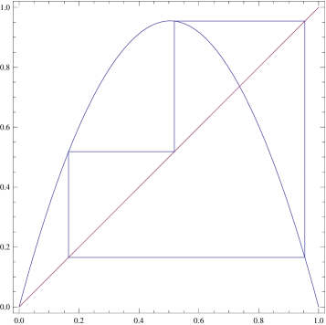
Figure 1. Period three saddle orbit generated by the fold bifurcation when $f^{3}$ crosses the diagonal in three points.

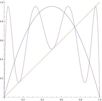
Figure 2. Triple tangency of the fold bifurcation for the implicit defined modified logistic.

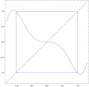
Figure 3. The period two orbit at the transcritical bifurcation point. This non-hyperbolic orbit is a saddle, attracting from the outside and repelling to the inside of the interval.

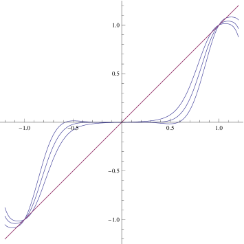
Figure 4. Double tangency of the transcritical bifurcation of period $2$ for the implicit dynamical system of example 4.2. We can see $f^{2}$ for values of the parameter near $2$. The periodic points cross stabilities.

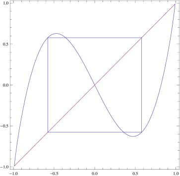
Figure 5. Non-hyperbolic orbit, although topologically stable, of period $2$ at the pitchfork bifurcation for the modified bimodal implicit dynamical system.

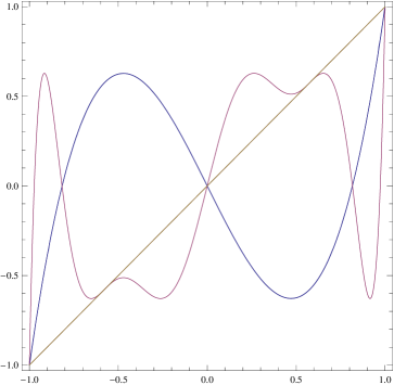
Figure 6. Double tangency of the pitchfork bifurcation of period $2$ for the implicit defined modified bimodal map. We can see $f$ and $f^{2}$.

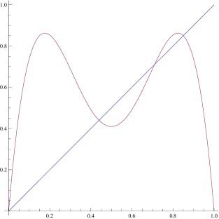
Figure 7. Flip bifurcation. We see the double intersection of the map $f^{2}$ with the diagonal. The map has slope $-1$ at the relevant intersections.

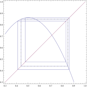
Figure 8. Flip bifurcation. We can see the attracting period $4$ orbit generated by the flip bifurcation and in the center the repelling period $2$ orbit obtained from the original attracting period $2$ orbit.

Example 4.1.

Fold case, period 3. Let be the implicitly defined discrete dynamical system for $x_{n}\in\left[0,1\right]$ and $\alpha\in\left[0,4\right]$, we call to the following model a modified implicit logistic map

$$F\left(x_{n},x_{n+1},\alpha\right)=x_{n+1}-\alpha x_{n}(1-x_{n}+\frac{x_{n+1}^{P}}{B})=0.$$

With $P=5$ and $B=100$, an explicit solution for $x_{n+1}$ is not possible, since the map

$$F\left(x,y,\alpha\right)=y-\alpha x(1-x+\frac{y^{5}}{100})=0,$$

does not admit a closed formula for the solution $y$. The derivatives of $F$ are

$$F_{x}\left(x,y,\alpha\right) =\alpha(-1+2x-\frac{y^{5}}{100}),$$

$$F_{y}\left(x,y,\alpha\right) =1-\frac{1}{20}\alpha xy^{4},$$

$$F_{\alpha}\left(x,y,\alpha\right) =-x(1-x+\frac{y^{5}}{100}),$$

$$F_{x^{2}}\left(x,y,\alpha\right) =2\alpha,$$

$$F_{y^{2}}\left(x,y,\alpha\right) =-\frac{\alpha xy^{3}}{5},$$

$$F_{xy}\left(x,y,\alpha\right) =-\frac{\alpha y^{4}}{20}.$$

We are looking for a period $3$ fold, the bifurcation equations are

$$\left\{\begin{array}[c]{l}F\left(x_{0},x_{1},\alpha\right)=0,\\ F\left(x_{1},x_{2},\alpha\right)=0,\\ F\left(x_{2},x_{0},\alpha\right)=0,\\ \partial_{x}f^{3}\left(x_{0}\right)=\left(-1\right)^{3}{\displaystyle\prod\limits_{j=0}^{2}}\frac{F_{x}\left(x_{j},x_{j+1\left(\operatorname{mod}3\right)}\right)}{F_{y}\left(x_{j},x_{j+1\left(\operatorname{mod}3\right)}\right)}=1.\end{array}\right.$$

A solution found numerically is

$$x_{0} =0.16498\ldots,x_{1}=0.51813\ldots,$$

$$x_{2} =0.954\ldots,\alpha=3.75938\ldots.$$

The previous computations show that there exists locally the implicitly defined discrete dynamical system, since the derivative $F_{y}\left(x,y,\alpha\right)$ does not vanish in the the interval $\left[0,1\right]$ containing the orbit. The non-degeneracy condition holds at the periodic orbit where $f=y$ is the implicitly defined iteration function

$$\partial_{x^{2}}f^{3}\left(x_{0}\right)=23.5\ldots\text{.}$$

The transversality condition gives

$$\partial_{\alpha}f^{3}\left(x_{0}\right)=-0.844\ldots\text{.}$$

Therefore, the bifurcation is a supercritical fold with period three, generating one period three attracting and one period three repelling orbits. The saddle orbit at the bifurcation point can be seen in Figure 1. The bifurcation is via a simultaneous triple tangency at the diagonal, and can be seen in Figure 2.

Example 4.2.

Transcritical case, period 2. Let be the implicitly defined discrete dynamical system for $x_{n}\in\left[0,1\right]$ and $\alpha\in\left[0,4\right]$

$$F\left(x_{n},x_{n+1},\alpha\right)=x_{n+1}+x_{n}+\alpha x_{n}\left(\left(x_{n}-\frac{x_{n+1}^{P}}{B}\right)^{2}-1\right)-x_{n}\left(\left(x_{n}-\frac{x_{n+1}^{P}}{B}\right)^{4}-1\right)=0.$$

With $P=3$ and $B=100$, an explicit solution for $x_{n+1}$ is not possible, since the equation

$$F\left(x,y,\alpha\right)=y+x-\alpha x\left(\left(x-\frac{y^{3}}{100}\right)^{2}-1\right)-x\left(\left(x-\frac{y^{3}}{100}\right)^{4}-1\right)=0,$$

does not admit a closed solution for $y$. At this point we omit the long computations needed and the list of derivatives, for sake of brevity. The reader can confirm our conclusions easily.

A period two solution for the transcritical bifurcation is found numerically to be

$$x_{0}=0.9903\ldots,x_{1}=-0.9903\ldots,\alpha=2.$$

There exists locally the implicitly defined discrete dynamical system, since the derivative $F_{y}\left(x,y,\alpha\right)$ does not vanish in the the interval $\left[0,1\right]$ containing the orbit. The non-degeneracy condition holds at the periodic orbit

$$\partial_{x^{2}}f^{2}\left(x_{0}\right)=-16.79\ldots\text{,}$$

the derivative relative to the parameter is

$$\partial_{\alpha}f^{2}\left(x_{0}\right)=0\text{.}$$

Therefore, the transversality condition is now

$$\partial_{\alpha x}f^{2}\left(x_{0}\right)=4.07769\text{.}$$

The conditions indicate a classical transcritical bifurcation, similar to the one that happens for the logistic map at the origin, but for a period two orbit. See Figures 3 and 4 for a graphical perspective of this type of bifurcation.

Example 4.3.

Pitchfork case, period 2. Let be the implicitly defined discrete dynamical system for $x_{n}\in\left[0,1\right]$ and $\alpha\in\left[0,4\right]$, we call to the following model a modified implicit bimodal map

$$F\left(x_{n},x_{n+1},\alpha\right)=x_{n+1}-\alpha\left(x_{n}+\frac{x_{n+1}^{P}}{B}\right)^{3}-\left(1-\alpha\right)\left(x_{n}+\frac{x_{n+1}^{P}}{B}\right)=0.$$

With $P=5$ and $B=100$, an explicit solution for $x_{n+1}$ is not possible, since the map

$$F\left(x,y,\alpha\right)=y-\alpha\left(x+\frac{y^{5}}{B}\right)^{3}-\left(1-\alpha\right)\left(x+\frac{y^{5}}{B}\right)=0,$$

does not admit a closed formula for the solution $y$. We are looking for a period $2$ pitchfork. The bifurcation equations are

$$\left\{\begin{array}[c]{l}F\left(x_{0},x_{1},\alpha\right)=0,\\ F\left(x_{1},x_{0},\alpha\right)=0,\\ \partial_{x}y^{2}\left(x_{0}\right)=\left(-1\right)^{2}{\displaystyle\prod\limits_{j=0}^{1}}\frac{F_{x}\left(x_{j},x_{j+1\left(\operatorname{mod}3\right)}\right)}{F_{y}\left(x_{j},x_{j+1\left(\operatorname{mod}3\right)}\right)}=1,\\ \partial_{x^{2}}y^{2}\left(x_{0}\right)=0.\end{array}\right.$$

For sake of brevity we do not present here the derivatives of $F$ but only the final results. A solution found numerically is

$$x_{0}=-0.5774599\ldots,x_{1}=0.5774599\ldots,\alpha=2.9989\ldots.$$

meaning that there exists a periodic orbit with period two that bifurcates. The first non-degeneracy condition holds at the periodic orbit

$$\partial_{x^{3}}y^{2}\left(x_{0}\right)=-295,6\ldots\text{.}$$

the first derivative in order to the parameter gives naturally

$$\partial_{\alpha}f^{2}\left(x_{0}\right)=0$$

and the transversality condition is now

$$\partial_{\alpha x}f^{2}\left(x_{0}\right)=4.05\ldots\text{.}$$

Therefore, the bifurcation is a supercritical pitchfork with period two, generating two new period two attracting orbits and the original period two attracting orbit becomes repelling. The orbit at the bifurcation point can be seen in Figure 5. The bifurcation is via a simultaneous double unfolding at the diagonal, and can be seen in Figure 6.

Example 4.4.

Flip case, period 2 into period 4. Let be the implicitly defined discrete dynamical system of example 4.1 for $x_{n}\in\left[0,1\right]$ and $\alpha\in\left[0,4\right]$

$$F\left(x,y,\alpha\right)=y-\alpha x(1-x+\frac{y^{5}}{100})=0,$$

The new derivatives of $F$ that matter are

$$F_{\alpha x}\left(x,y,\alpha\right) =-1+2x-\frac{y^{5}}{100},$$

$$F_{\alpha y}\left(x,y,\alpha\right) =-\frac{xy^{4}}{20},$$

$$F_{x^{3}}\left(x,y,\alpha\right) =0,$$

$$F_{x^{2}y}\left(x,y,\alpha\right) =0,$$

$$F_{xy^{2}}\left(x,y,\alpha\right) =-\frac{\alpha y^{3}}{5}$$

$$F_{y^{3}}\left(x,y,\alpha\right) =-\frac{3\alpha xy^{2}}{5}.$$

We are looking for a period $2$ flip that bifurcates in a period $4$, the bifurcation equations are for $x_{0}\not=x_{1}$

$$\left\{\begin{array}[c]{l}F\left(x_{0},x_{1},\alpha\right)=0,\\ F\left(x_{1},x_{0},\alpha\right)=0,\\ \partial_{x}f^{2}\left(x_{0}\right)=\left(-1\right)^{2}{\displaystyle\prod\limits_{j=0}^{1}}\frac{F_{x}\left(x_{j},x_{j+1\left(\operatorname{mod}3\right)}\right)}{F_{y}\left(x_{j},x_{j+1\left(\operatorname{mod}3\right)}\right)}=-1.\end{array}\right.$$

A solution found numerically is

$$x_{0}=0.8466\ldots,x_{1}=0.4427\ldots,\alpha=3.405\ldots.$$

The previous computations show that there exists locally the implicitly defined discrete dynamical system, since the derivative $F_{y}\left(x,y,\alpha\right)$ does not vanish in the the interval $\left[0,1\right]$ containing the orbit. The non-degeneracy condition (10) holds at the periodic orbit where $f$ is the implicitly defined iteration function

(23) $$\frac{1}{2}\left(f_{x^{2}}^{2}\left(x_{0}\right)\right)^{2}+\frac{1}{3}f_{x^{3}}^{2}\left(x_{0}\right)=1383.1\not=0,$$

which is equivalent to say that the Schwarzian derivative of $f^{2}$ is not zero at $x_{0}$. The transversality condition (11) is

(24) $$f_{x\alpha}^{2}(x_{0})=1.45122\not=0\text{.}$$

Therefore, the bifurcation is a supercritical flip from period two to period four, generating one period four attracting and one period two repelling orbits. The bifurcation is via a simultaneous double $-1$ derivative for $f^{2}$ at the diagonal, and can be seen in Figure 7, finally in Figure 8 we can see the orbits after the bifurcation, the dotted line is the period two repelling orbit.

4.0.1. Bifurcations in backward Euler and trapezoid methods

Consider the autonomous differential equation

(25) $$x^{\prime}\left(t\right)=G\left(x\left(t\right)\right)\text{, }x\left(0\right)=x_{0}\text{.}$$

In the usual Euler method the integral is estimated at the leftmost point of each interval giving

(26) $$x_{n+1}-x_{n}=hG\left(x_{n}\right),$$

where $h$ is a positive real number, possibly very small. The backward, or implicit Euler method [10, 11], where the integral is estimated using the rightmost point of each interval $x_{n+1}$ gives the iterative scheme

(27) $$x_{n+1}-x_{n}=hG\left(x_{n+1}\right).$$

Actually this is a very simple one-dimensional discrete dynamical system, obviously it can depend on internal parameters in $G$, but we are interested in considering $h$ as the bifurcation parameter.

The iterative scheme is given by

(28) $$F\left(x_{n},x_{n+1}\right)=x_{n+1}-x_{n}-hG\left(x_{n+1}\right)=0.$$

Our function $F$ is

(29) $$F\left(x,y\right)=y-x-hG\left(y\right).$$

The original Euler method is considered explicit since in that case $y=x+hG\left(x\right)$ and $x_{n+1}=x_{n}+hG\left(x_{n}\right)$.

In the case of the trapezoid method [10] (which is a second order method) we have for the same differential equation the iterative scheme

(30) $$F\left(x_{n},x_{n+1}\right)=x_{n+1}-x_{n}-\frac{h}{2}\left(G\left(x_{n+1}\right)+G\left(x_{n}\right)\right)=0$$

and the function $F$ is

(31) $$F\left(x,y\right)=y-x-\frac{h}{2}\left(G\left(y\right)+G\left(x\right)\right)\text{,}$$

this method is intrinsically implicit, since there is no immediate solution of $F\left(x,y\right)=0$ for $y$. We consider now the existence of periodic orbits in the Euler iteration, the period is $p$, the simplest case is the asymptotic stable fixed point, which indicates that the solution of the original differential equation has a limit when $t$ goes to infinity for a set of initial conditions. Obviously the non-hyperbolic condition (17b) for the backward Euler method simplifies

$$\partial_{x}f^{p}\left(x_{0}\right)=\frac{1}{{\displaystyle\prod\limits_{j=0}^{p-1}}\left(1-hG^{\prime}\left(x_{j+1\left(\operatorname{mod}p\right)}\right)\right)}=\pm 1,$$

this gives the non hyperbolic conditions for the backward Euler method

(32) $${\displaystyle\prod\limits_{j=0}^{p-1}}\left(1-hG^{\prime}\left(x_{j}\right)\right)=\pm 1\text{.}$$

For the trapezoid method the non-hyperbolic condition (17b) is

$${\displaystyle\prod\limits_{j=0}^{p-1}}\frac{1+\frac{h}{2}G^{\prime}\left(x_{j}\right)}{1-\frac{h}{2}G^{\prime}\left(x_{j}\right)}=\pm 1\text{.}$$

The non-degeneracy condition (19) is

$$\partial_{h}f^{p}\left(x_{0}\right)=\left(-1\right)^{p}{\displaystyle\sum\limits_{j=0}^{p-1}}\frac{\left(-1\right)^{j}F_{h}\left(x_{j},x_{j+1}\right)}{F_{y}\left(x_{j},x_{j+1}\right)}{\displaystyle\prod\limits_{i>j}^{p-1}}\frac{F_{x}\left(x_{i},x_{i+1}\right)}{F_{y}\left(x_{i},x_{i+1}\right)}\not=0.$$

For the backward Euler method it gives

$${\displaystyle\sum\limits_{j=1}^{p}}{\displaystyle\prod\limits_{i\geq j}^{p}}\frac{G\left(x_{j}\right)}{\left(1-hG^{\prime}\left(x_{i}\right)\right)}\not=0\text{, with }x_{p}=x_{0}.$$

For the trapezoid method we have

$$\frac{1}{2}{\displaystyle\sum\limits_{j=0}^{p-1}}\frac{\left(-1\right)^{j}\left(G\left(x_{j}\right)+G\left(x_{j+1}\right)\right)}{1-\frac{h}{2}G^{\prime}\left(x_{j+1}\right)}{\displaystyle\prod\limits_{i>j}^{p-1}}\frac{1+\frac{h}{2}G^{\prime}\left(x_{i}\right)}{1-\frac{h}{2}G^{\prime}\left(x_{i+1}\right)}\not=0\text{, with }x_{p}=x_{0}.$$

We study a simple example for the backward Euler method. Similar examples can be constructed for the trapezoid method.

Example 4.5.

Consider the simple differential equation

(33) $$x^{\prime}=x^{5}-1\text{, }x_{0}=0\text{.}$$

This equation can be solved by quadratures but it is impossible to obtain an explicit expression for the solution. Applying Euler backward method we get

$$x_{n+1}-x_{n}=hx_{n+1}^{5}-h\text{,}$$

i.e.,

$$F\left(x_{n},x_{n+1}\right)=x_{n+1}-x_{n}-h\left(x_{n+1}^{5}-1\right)=0\text{.}$$

Naturally, $G\left(y\right)=y^{5}-1$. We have $G^{\prime}\left(y\right)=-5y^{4}$. Equation (32) is

(34) $${\displaystyle\prod\limits_{j=0}^{p-1}}\left(1-5hx_{j}^{4}\right)=\pm 1\text{.}$$

We have to solve (14) together with (34), we start by the fixed point

$$\left\{\begin{array}[c]{l}x_{0}^{5}-1=0,\\ \left(1-5hx_{0}^{4}\right)=\pm 1\text{.}\end{array}\right.$$

Excluding the trivial case $x=1$, $h=0$, there are no solutions for the fold case. The solution is fairly simple for the flip case

$$x_{0}=1\text{, }h=0.4\text{,}$$

This means that when $h=0.4$ the fixed point $x_{0}=1$ duplicates. When $h$ is greater than $0.4$ the fixed point becomes attracting and is generated a period two repelling orbit. Below $0.4$ the fixed point $x_{0}=1$ is repelling.

Now let us consider a period two orbit, the bifurcation equations are now

$$\left\{\begin{array}[c]{l}x_{1}-x_{0}=hx_{1}^{5}-h\\ x_{0}-x_{1}=hx_{0}^{5}-h\\ \left(1-5hx_{0}^{4}\right)\left(1-5hx_{1}^{4}\right)=\pm 1\text{.}\end{array}\right.$$

We get, among complex solutions not considered here, the non trivial ($h\not=0$) real solutions for the fold case

$$x_{0} =x_{1}=1\text{, }h=0.4\text{, degenerate and obtained previously }$$

$$x_{0} =1.15767\text{, }x_{1}=-0.602341\text{, }h=1.63071\text{.}$$

obviously $x_{0}=-0.602341$ and $x_{1}=1.15767$ is also a solution.

For the flip case we get the period doubling point where a period two orbit duplicates its period

$$x_{0} =1.12579,\text{ }x_{1}=0.718620,\text{ }h=0.503700,$$

$$x_{0} =-0.580682,\text{ }x_{1}=1.15618,\text{ }h=1.62930.$$

This means that the previously created at $h=0.4$ repelling period two solution, bifurcates again when $h=0.503700$ to a period $4$ orbit.

Finally, among other period three solutions, there is a period three fold at a low value of $h$

$$x_{0}=0.784072,\text{ }x_{1}=0.16453,\text{ }x_{2}=1.22008,\text{ }h=0.619616.$$

Due to the continuity of all the functions involved this implies the existence of chaos for low values of the parameters, even in the case of the backward Euler method of a very simple first order differential equation. It is a well known fact that one-dimensional discrete dynamical systems are more complex than one-dimensional continuous dynamical systems. Nevertheless, the existence of chaos for small values of the parameter $h$ is still exciting.

The previous example suggests the existence of a plethora of phenomena deserving further research in implicit numeric methods. By force, the more general cases of implicit discrete dynamical systems, which are very scarce in the literature, are a vast field of research totally open.

Acknowledgement Partially funded by FCT/Portugal through UID/MAT/04459/ 2013 for CMAGDS.

References

• [1] D. J. Allwright, Hypergraphic functions and bifurcations in recurrence relations, Siam Journal on Applied mathematics 34 (4) (1978) 687–691.
• [2] V. I. Arnold, Dynamical Systems. V. Bifurcation Theory and Catastrophe Theory, Encyclopedia of Mathematical Sciences, vol. 5 of Encyclopaedia of Mathematical Sciences, Springer, Berlin, 1994.
• [3] S. Chow, J. Hale, Methods of Bifurcation Theory, vol. 251, Springer, 1982.
• [4] P. Collet, J. P. Eckman, Iterated Maps of the Interval as Dynamical Systems, Springer, New York, 1980.
• [5] A. Dávid, S. Sinha, Versal deformation and local bifurcation analysis of time-periodic nonlinear systems, Nonlinear Dynamics 1 (4) (2000) 317–336.
• [6] A. A. Davydov, G. Ishikawa, S. Izumiya, W.-Z. Sun, Generic singularities of implicit systems of first order differential equations on the plane, Japanese Journal of Mathematics 3 (1) (2008) 93–119.
• [7] C.-I. Gheorghiu, On some one-step implicit methods as dynamical systems, Revue d’Analyse Numerique et de Theorie de l’Approximation 32 (2) (2003) 171–176.
• [8] M. Golubitsky, D. Schaeffer, Singularities and Groups in Bifurcation Theory, vol. 51, Applied Mathematical Sciences, 1985.
• [9] J. Guckenheimer, On the bifurcation of maps of the interval, Inventiones mathematicae 39 (2) (1977) 165–178.
• [10] E. Hairer, S. P. Nrsett, G. Wanner., Solving Ordinary Differential Equations I: Nonstiff Problems, vol. 8 of Springer Series in Computational Mathematics, 2nd ed., Springer, Berlin, New York, Heidelberg, 2009.
• [11] E. Hairer, G. Wanner., Solving Ordinary Differential Equations II: Stiff and Differential-Algebraic Problems, vol. 14 of Springer Series in Computational Mathematics, 2nd ed., Springer, Berlin, New York, Heidelberg, 1996.
• [12] K. Hirai, T. Adachi, Chaos and bifurcation in numerical computation by the Runge-Kutta method, International Journal of Systems Science 25 (11) (1994) 1695–1706.
• [13] J. Holl, K. Schlacher, Analysis and nonlinear control of implicit discrete-time dynamic systems, IFAC Proceedings 38 (1) (2005) 145–150.
• [14] J. Kennedy, D. R. Stockman, J. A. Yorke, Inverse limits and an implicitly defined difference equation from economics, Topology and its Applications 13 (154) (2007) 2533–2552.
• [15] W. Kleczka, E. Kreuzer, On the systematic analytic-numeric bifurcation analysis, Nonlinear Dynamics 7 (2) (1995) 149–163.
• [16] S. G. Krantz, H. R. Parks, The Implicit Function Theorem: History, Theory, and Applications, Springer, Berlin, Heildelberg, 2012.
• [17] I. A. Kuznetsov, Elements of Applied Bifurcation Theory, vol. 112, 3rd ed., Springer, New York, Berlin, Heidelberg, 1998.
• [18] C.-H. Lamarque, J. Bastien, Numerical study of a forced pendulum with friction, Nonlinear Dynamics 23 (4) (2000) 335–352.
• [19] R. Lozi, J. Sousa-Ramos, A. Sharkovsky, One-dimensional dynamics generated by boundary value problems for the wave equation, Grazer Math. Berlin (346) (2004) 255–270.
• [20] A. C. J. Luo, Discretization and Implicit Mapping Dynamics, Nonlinear Physical Science, Springer, New York, Berlin, Heildelberg, 2015.
• [21] A. Medio, B. Raines, Backward dynamics in economics, the inverse limit approach, Journal of Economic Dynamics and Control 31 (5) (2003) 1633–1671.
• [22] A. Medio, B. Raines, Implicit equilibrium dynamics., Macroeconomic Dynamics 16 (4) (2012) 518–555.
• [23] I. Mezić, Spectral properties of dynamical systems, model reduction and decompositions, Nonlinear Dynamics 41 (1) (2005) 309–325.
• [24] H. Oliveira, Invariance of bifurcation equations for high degeneracy bifurcations of non-autonomous periodic maps, Topological Methods in Nonlinear Analysis 42 (2) (2016) 715–737, doi: 10.12775/TMNA.2016.031.
• [25] G. Rega, H. Troger, Dimension reduction of dynamical systems: Methods, models, applications, Nonlinear Dynamics 41 (1) (2005) 1–15.
• [26] R. Severino, J. Sousa-Ramos, A. Sharkovsky, S. Vinagre, Symbolic dynamics in boundary value problems, Grazer Math. Berich (346) (2004) 393–402.
• [27] R. Severino, J. Sousa-Ramos, A. Sharkovsky, S. Vinagre, Symbolic dynamics in boundary value problem for systems with two spatial variables, Grazer Math. Berich (350) (2006) 210–224.
• [28] A. Sharkovsky, G. Pelyukh, Invariant Methods in the Theory of Functional Equations (in Ukrainian), vol. 95, Proceedings of the Mathematical Institute of the Academy of Sciences of Kiev, Kiev, 2013.
• [29] T. Ushio, K. Hirai, Chaos induced by the generalized Euler method, International Journal of Systems Science 17 (4) (1986) 669–678.
• [30] L. Zhang, D. Zhang, A two-loop procedure based on implicit Runge–Kutta method for index-3 dae of constrained dynamic problems, Nonlinear Dynamics 85 (1) (2016) 263–280.