A global view of velocity fluctuations in the corona below 1.3 $R_{\odot}$ with CoMP

Abstract

The Coronal Multi-channel Polarimeter (CoMP) has previously demonstrated the presence of Doppler velocity fluctuations in the solar corona. The observed fluctuations are thought to be transverse waves, i.e. highly incompressible motions whose restoring force is dominated by the magnetic tension, some of which demonstrate clear periodicity. We aim to exploit CoMP’s ability to provide high cadence observations of the off-limb corona to investigate the properties of velocity fluctuations in a range of coronal features, providing insight into how(if) the properties of the waves are influenced by the varying magnetic topology in active regions, quiet Sun and open fields regions. An analysis of Doppler velocity time-series of the solar corona from the $10,747$ Å Iron XIII line is performed, determining the velocity power spectra and using it as a tool to probe wave behaviour. Further, the average phase speed and density for each region are estimated and used to compute the spectra for energy density and energy flux. In addition, we assess the noise levels associated with the CoMP data, deriving analytic formulae for the uncertainty on Doppler velocity measurements and providing a comparison by estimating the noise from the data. It is found that the entire corona is replete with transverse wave behaviour. The corresponding power spectra indicates that the observed velocity fluctuations are predominately generated by stochastic processes, with the spectral slope of the power varying between the different magnetic regions. Most strikingly, all power spectra reveal the presence of enhanced power occurring at $\sim 3$ mHz, potentially implying that the excitation of coronal transverse waves by $p$-modes is a global phenomenon.

1. Introduction

There is currently significant interest in MHD waves in the solar atmosphere and whether they transport enough energy to play a significant role in solar atmospheric heating and the acceleration of the solar wind (see, e.g., the following reviews and references within, Narain & Ulmschneider, 1996, Klimchuk, 2006, Erdélyi & Ballai, 2007, Matthaeus & Velli, 2011, Parnell & De Moortel, 2012, Cranmer, 2012, Hansteen & Velli, 2012). Enthusiasm for wave-based theories of heating and acceleration has been renewed in recent years, with observations suggesting the presence of transverse waves in many distinct plasma structures defined by the magnetic field in both the corona and the chromosphere (e.g., De Pontieu et al., 2007b, Okamoto et al., 2007, Tomczyk et al., 2007, Erdélyi & Taroyan, 2008, Morton et al., 2012, 2013, Pereira et al., 2012, Hillier et al., 2013, Nisticò et al., 2013, Thurgood et al., 2014).

In complex magnetised plasmas, such as the solar chromosphere and corona, MHD waves cannot typically be characterised as purely Alfvén or purely fast modes, but have mixed properties (although there are exceptions such as the $n=0$ torsional Alfvén wave, e.g., Spruit, 1982). The kink wave is one example of a transverse wave mode with mixed properties (see, e.g., Spruit, 1982, Edwin & Roberts, 1983, Goossens et al., 2009, 2012). The properties of the kink wave vary depending on the ratio of the wavelength ($\lambda$) to the radius ($r$) of the magnetic flux tube that supports the wave. In the so called Thin Tube (TT) limit, when $r<<\lambda$, the kink wave has the following properties: (i) high incompressibility; (ii) the ability to transport vorticity; (iii) the dominance of magnetic tension as the restoring force (Goossens et al., 2009, 2012).

Current instrumentation indicates that the chromosphere and corona is finely structured, with typical transverse scales of $\sim 400$ km (De Pontieu et al., 2007a, Morton et al., 2012, Brooks et al., 2013, Morton & McLaughlin, 2013, 2014, Winebarger et al., 2014). The fine-scale structure is seen to support MHD waves, and theoretical considerations demonstrate that these (likely) over dense magnetic flux tubes act as waveguides, funnelling the wave energy through the solar atmosphere. The propagation speeds of observed kink waves are typically in excess of 50 km s^-1 in the chromosphere (Jess et al., 2015) and $200$ km s^-1 in the corona (Tomczyk et al., 2007; Morton et al., 2015). Further, periods have been observed as short as 40 s (He et al., 2009, Morton & McLaughlin, 2013), although periods of 100 s-500 s are more usual with current observational capabilities. Hence, for a somewhat typical case with $r=400$ km, $c_{p}=100$ km s^-1 and $P=100$ s, the ratio $r/\lambda=r/(c_{p}P)\sim 0.04$. This would imply that the currently observable kink modes lie in the TT regime where the wave displays their incompressible qualities.

Previous observations of transverse waves have largely been through imaging observations, revealing the ubiquity of kink motions characterised by the non-axisymmetric displacement of flux tubes. These observations have been ideal for establishing the existence of such wave modes and also providing estimates for their typical properties (amplitudes, periods) in the different magnetic environments. McIntosh et al. (2011) demonstrated that the transverse waves are found in active regions, the quiet Sun and coronal holes, and further suggested that typical amplitudes are greater in the coronal holes and smaller in active regions, with periods between 100-500 s. Similar results are found for chromospheric features (Pereira et al., 2012, Morton et al., 2014, Jess et al., 2015).

Even after numerous observations of these waves, major uncertainties about their contribution to energy transfer still remain. For example, it is still unclear exactly what role the observed waves play (if any) in heating the solar atmosphere. While estimates for the energy content (and flux) of the waves have been given, the values are still subject to a great deal of uncertainty from both observational (e.g., van Doorsselaere et al., 2008, McIntosh et al., 2011, Morton & McLaughlin, 2013, Nisticò et al., 2013, Thurgood et al., 2014) and theoretical standpoints (Goossens et al., 2013, Van Doorsselaere et al., 2014).

Now that the presence of the transverse waves in the solar atmosphere has been established, the focus of wave observations should shift to measuring other attributes that can be used for testing current wave-based theories. Although, this may be an onerous task with imaging observations. The typical process of measurement, at present, is relatively cumbersome and time-intensive, however, it can provide well-constrained measurements. Some progress has been made towards this goal though. For example, Hillier et al. (2013) and Morton et al. (2014) derived velocity power spectra for kink waves in prominences and fibrils respectively, allowing for an initial comparison to the velocity power spectra derived from motions of granules and magnetic bright points. The results suggested an apparent correlation between the spectra hinting the waves may be driven by the photospheric motions (see also, Stangalini et al., 2013, 2014, 2015). The generation of incompressible waves by the turbulent convective motions in the photosphere has been a long held belief (e.g., Osterbrock, 1961) and typically is the driving mechanism for transverse waves in models of heating and wind acceleration.

Observations that allow for Doppler diagnostics, such as those with the Coronal Multi-Channel Polarimeter (CoMP - Tomczyk et al., 2008) provide a significant advantage over imaging observations in the fact that it is less arduous to generate power spectra. The sampling of particular spectral lines allows the measurement of both Doppler velocities and Doppler widths, providing time-series of these quantities. CoMP, at present, is unique in providing a global view of the corona with the required spectral resolution to provide high cadence time-series of velocity fluctuations. CoMP data has been used previously to provide a focused look at kink wave propagation in individual features e.g., Tomczyk & McIntosh (2009); Threlfall et al. (2013), De Moortel et al. (2014).

One of the interesting features observed in the CoMP data is the appearance of an enhancement of power, centred on 3 mHz, found in a quiescent loop and an open field region (Tomczyk et al., 2007, Morton et al., 2015). The coronal magnetic fields are generally considered to be rooted in kilo-gauss faculae that form the network and plage regions in the photosphere (Gabriel, 1976, Dowdy et al., 1986, Peter, 2001), possibly apart from active region features which can emanate from pores and sunspots. Studies of the interaction and scattering of acoustic waves with flux tubes suggest the concentrations of photospheric magnetic flux provide waveguides for p-modes to leak out from the interior into the lower solar atmosphere (Schunker & Cally, 2006, Jain et al., 2011, Gascoyne et al., 2014). The magneto-acoustic waves can propagate higher into the solar atmosphere, eventually reaching a canopy where the Alfvén speed equals the sound speed. At this canopy mode coupling occurs and the magneto-acoustic energy is split between both slow and fast magneto-acoustic waves, with the proportion dependent upon the angle of the magnetic field, e.g., Bogdan et al. (2003), Khomenko & Collados (2006), Khomenko et al. (2008), Vigeesh et al. (2009), Fedun et al. (2009, 2011). While, slow modes above this canopy are expected to steepen and shock due to the rise in temperature in the upper chromosphere (as evidenced by the dynamics of type-I spicules, e.g., De Pontieu et al., 2004), the fast magneto-acoustic waves can be reflected due to the steep gradient in Alfvén speed at the transition region. Theoretical and numerical modelling of wave propagation in a simplified atmosphere have shown, under certain conditions, there is a coupling of the fast wave to the Alfvén wave, enabling wave energy to cross the transition region and propagate into the corona as Alfvén waves. (Cally & Goossens, 20008, Cally & Hansen, 2011, Cally, 2011, Khomenko & Cally, 2012, Hansen & Cally, 2012). This process by its very nature must generate vorticity, which has to propagated through an inhomogeneous corona implying, in principle, that it could excite kink waves. Using a relatively simple model atmosphere, Hansen & Cally (2012) estimate that a sufficient amount of energy can be converted from p-modes to coronal Alfvén waves to explain the estimated energy content of observed kink motions in the corona. Due to the ubiquity of small-scale magnetic features across the solar surface and the global nature of $p$-modes, it may be expected that this phenomenon is widespread through the atmosphere.

In the following, CoMP data is utilised to investigate the properties of velocity fluctuations globally in the corona. The main diagnostic to achieve this is the velocity power spectrum, which is derived for typical coronal regions, i.e., quiet Sun, active, and open field regions. Each region is found to have spectra with qualitatively similar properties, with steep spectral slopes and power enhancements at $3$ mHz. It is evident that the power enhancement is present throughout the corona and confirms its global nature. However, each spectra has distinct power laws and the magnitude of the power also varies between the regions. The measured flux of wave energy density and flux are found to be inhomogeneous through the corona, with the greatest flux energy in the quiescent regions. To complement the analysis, we derive analytic formula for the errors related to the analytic fits used for the CoMP data products, which enables us to assess the limitations of the CoMP observations.

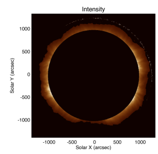
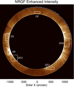
Figure 1.— The CoMP field of view on the 27 March 2012 at 18:51:02 UT. The left hand panel displays the line centre intensity, which is scaled in millionths of the solar disk intensity. The right hand panel shows the intensity enhanced by a NRGF filter, revealing some of the fine scale structure in the corona. The pixels used to obtain the average power spectra (see, Figure 6) are highlighted by the boxes, for typical coronal features, i.e. an open field region (OF), the quiet Sun (QS) and active region (AR). An additional three quiet Sun region (QS 2-4) are examined in Figure 7.

2. Observations and data reduction

The data used here were obtained with the CoMP on the 27 March 2012 at 18:51:02 UT to 20:13:02 UT. The details of the acquisition and reduction of CoMP data are fully described in Tomczyk et al. (2008) and we make use of the final data product that has a cadence of $30$ s and a pixel size of $4".46$. We note the individual frames in the final data product are produced by averaging over 16 consecutive images. The final data products are intensity images of the corona at three wavelengths (10745.0 Å - $I_{1}$, 10746.2 Å - $I_{2}$ and 10747.4 Å - $I_{3}$), which are positions centred on the 10747 Å FeXIII emission line (peak formation temperature of $\sim 1.6$ MK in ionisation equilibrium). Following Tian et al. (2013), for each pixel in the CoMP field of view in each time frame we calculate the central intensity, Doppler velocity shift and Doppler width of the line profile using an analytic fit of a Gaussian to the intensity values at each wavelength position. The equations for these quantities are

$$v = \frac{w^{2}}{4d}(a-b),$$ (1)

$$w = \sqrt{\frac{-2d^{2}}{a+b}},$$ (2)

$$i = I_{2}\exp{\frac{v^{2}}{w^{2}}},$$ (3)

where $v$ is the Doppler velocity, $w$ is the Doppler width and $i$ is the line centre intensity. The $a$ and $b$ are functions of $I_{1},I_{2},I_{3}$, namely,

$$a=\ln{\frac{I_{3}}{I_{2}}},\qquad b=\ln{\frac{I_{1}}{I_{2}}}$$ (4)

and $d$ is the spectral step size. For the Doppler velocity time-series, the solar rotation is removed in the manner suggested in Tian et al. (2013).

This is the same data set used in Bethge et al. (2016). It consists of 164 images, almost uninterrupted. One image at 19:59:33 UT was of low quality so was replaced by an image interpolated from the neighbouring images in the time-series. An example image from the data set showing the CoMP field of view is shown in Figure 1. In addition, the figure shows an image at 10746.2 Å that has been enhanced with a normalising radial gradient filter (NRGF) to allow some of the coronal structures to be better visualised.

The central intensity images are then aligned using cross-correlation and the same shifts are applied to the Doppler velocity images. The results of the cross-correlation suggest that the residual motions of the co-aligned data is less than 0.1 pixels.

Further, before the main series of data were taken, a sequence of five-point line scans for the full field of view were taken from 17:44:56 UT to 18:46:14 UT, alternating between the FeXIII lines at $10747$ Å and $10798$ Å. For each emission line scan, the intensities are fit with a Gaussian, allowing the line core intensity to be estimated. These line core intensities will be used for density diagnostics.

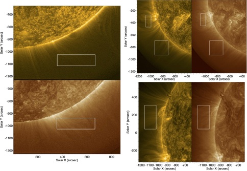
Figure 2.— High resolution SDO/AIA images showing coronal emission in 171 Å (left panels) and 193 Å (right panels). The images reveal the magnetic topology of the regions analysed with CoMP. The left hand panels show QS2, the top right hand panels shows AR and QS3, the bottom right panels show QS. The images have been subject to an MGN filter (Morgan & Druckmüller, 2014) to enhance the fine-scale structure.

In the following we will investigate velocity fluctuations throughout the corona. Regions with varying magnetic geometries and field strengths, i.e., open field region (OF), quiet Sun (QS, QS2, QS3, QS4) and active region (AR) are selected in CoMP images. The identification of regions is aided with coronal data from the Solar Dynamics Observatory (SDO - Pesnell et al., 2012) Atmospheric Imaging Assembly (AIA - Lemen et al., 2012) and magneto-grams from the Helioseismic and Magnetic Imager (HMI - Scherrer et al., 2012) that reveal the photospheric magnetic flux, which also allow for estimates of the field line connectivity using PFSS extrapolations (Schrijver & De Rosa, 2003). The magneto-grams and extrapolations are not shown.

Six regions in the corona are selected for analysis and are chosen as they are representative of active, open field and quiet Sun regions. These regions are highlighted by boxes in Figure 1. In Figures 2 and 3, data from SDO/AIA is presented that provides a high resolution (0”.6/pixel) view of the corona in the 171 Å and 193 Å bandpasses. The images reveal the fine-scale magnetic structure of the active region (11448) and the quiet Sun regions that are highlighted by the boxes in Figure 1. The open field region is analysed in Morton et al. (2015) so we will not discuss the details here.

The first panels in Figure 2 show a quiet Sun region (QS2) located near the southern pole, which demonstrates that the local magnetic field is composed of both closed and open magnetic structures (the term open is used to refer to magnetic fields that reach the source surface in the PFSS extrapolation). No large scale magnetic flux features are evident in magneto-grams from the preceding days.

The second panels show the active region (AR 11448) located at the limb, which displays a complicated mass of coronal loop structures. Magneto-grams from the proceeding days show the active region rotating onto the disk and reveal a bipolar magnetic flux concentration that is predominantly east-west orientated, in which the loops are rooted. This implies that AIA and CoMP are observing the loops end on, as opposed to the loops being in the plane of sky. There is also a quiet Sun region (QS3) to the south of the active region with a cusp-like structure. Some of the more northern magnetic field associated with this structure may be rooted in a unipolar region that lies close to the active region, but the southern magnetic field emanates from a magnetically quiet region, similar to that of the first quiet Sun feature.

The third set of panels in Figure 2 display a third quiet Sun region (QS). The magnetic field in this region is predominantly open, although its appearance isn’t radial like the fields in the other two quiet Sun regions. The magnetic fields originate from two patches of unipolar network magnetic field with opposite polarity. The PFSS extrapolation of the magnetic field in the corona suggests that the closed loops seen clearly in $171$ Å have a footpoint in each of these patches.

The final region (QS4) is shown in Figure 3. The feature of interest is an arcade of trans-equatorial coronal loops that are almost in the plane of sky. The loops have their southern footpoints located close to a decaying active region (11436) and their northern footpoints close to a patch weak unipolar field. There is a region between the two where no distinct large-scale photospheric magnetic structure is visible. The exact location for each set of footpoints is difficult to distinguish, with the coronal loops in $193$ Å having higher/lower latitude footpoints (for northern/southern hemisphere footpoints) to the loops visible in $171$ Å.

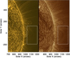
Figure 3.— Similar to Figure 2 but showing the region QS4.

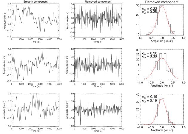
Figure 4.— Estimating the noise from the data. Three examples of Doppler velocity time-series from single pixels are separated into the signal (first column) and noise (second column). A histogram of the removed signal is fit with a Gaussian (red line) and the standard deviation of the measured noise, $\sigma_{M}$, is given. This can be compared to the analytic estimate for the noise, $\sigma_{A}$.

3. Determining CoMP noise levels

In the following, estimates for the errors on CoMP measurements will be calculated in order to evaluate constraints on results derived here and in future studies. First, analytic formulae are derived to estimate the uncertainties associated with the Doppler velocities, which are then compared to measurements of noise from the data.

3.1. Uncertainties on the measurable quantities

The errors on the intensities $I_{1},I_{2},I_{3}$, used for the analytic Gaussian fit, requires an estimate of the data noise ($\sigma_{N}$), which is given by

$$\sigma_{N}^{2}={\sigma_{p}(F)^{2}+\sigma_{d}^{2}+\sigma_{f}^{2}+\sigma_{bck}^{2}(F)+2\sigma_{r}^{2}+\sigma_{sd}^{2}+\sigma_{see}(F)^{2}},$$ (5)

where $\sigma_{p}(F)$ is the uncertainty due to photon noise, $\sigma_{d}$ is the dark current, $\sigma_{f}$ the flat field, $\sigma_{bck}(F)$ is the photospheric continuum background subtraction, $\sigma_{r}$ the readout (factor of two for coronal emission and photospheric background), $\sigma_{sd}$ the digitisation and $\sigma_{see}(F)$ is the seeing noise. The $F$ indicates the noise level is dependent on the intensity flux.

Each time frame of $I_{1},I_{2},I_{3}$ are a product of averaging over a number of exposures, hence, the data noise can be divided by the square root of the number of exposures, i.e., sixteen. It is likely that the photon noise, the background subtraction and the seeing will dominate the noise. The uncertainties associated with the flat and dark noise are small and can be neglected after the averaging. While we are able to confidently provide the uncertainties for photon, background and read noise, it is much more difficult to assess the magnitude of the seeing noise. It is expected that the seeing noise is proportional to the intensity gradient, i.e.,

$$\sigma_{see}^{2}=\left(\frac{dI}{dz}\right)^{2}\sigma_{z}^{2},$$ (6)

where $dI/dz$ is the spatial derivative of the intensity and $\sigma_{z}$ is the uncertainty due to the seeing. With respect to $\sigma_{z}$, a value of $0.1$ pixels is used, in line with estimates of the residual motions from the cross-correlation (for a discussion see Appendix A).

Having calculated a measure of the uncertainty for the intensity, the uncertainty on the velocity is obtained from the standard error propagation formula

$$\delta X^{2}=\sum\limits_{i}\left(\frac{\partial X}{\partial x_{i}}\delta x_{i}\right)^{2},$$ (7)

where $X$ is the calculated quantity, $\delta X$ is the associated uncertainty (standard deviation), $x_{i}$ are the independent quantities and $\delta x_{i}$ is their uncertainty.

The Doppler velocity is defined as

$$v=-\frac{d}{2}\frac{a-b}{a+b}=-\frac{d}{2}\frac{\ln{\frac{I_{3}}{I_{2}}}-ln{\frac{I_{1}}{I_{2}}}}{ln{\frac{I_{3}}{I_{2}}}+ln{\frac{I_{1}}{I_{2}}}},$$ (8)

which can be re-written as

$$v=-\frac{d}{2}\frac{\ln{{I_{3}}}-\ln{{I_{1}}}}{-2\ln{I_{2}}+\ln{I_{3}}+\ln{I_{1}}}.$$ (9)

Taking the partial derivatives of Eq. 9 with respect to the measured intensities, we obtain

$$\frac{\partial v}{\partial I_{1}} = \frac{d}{2I_{1}(-2\ln{I_{2}}+\ln{I_{3}}+\ln{I_{1}})}$$ (10)

$$+\frac{d(\ln{I_{3}}-\ln{I_{1}})}{2I_{1}(-2\ln{I_{2}}+\ln{I_{3}}+\ln{I_{1}})^{2}}$$

$$\frac{\partial v}{\partial I_{2}} = -\frac{d(\ln{I_{3}}-\ln{I_{1}})}{I_{2}(-2\ln{I_{2}}\ln{I_{3}}+\ln{I_{1}})^{2}}$$ (11)

$$\frac{\partial v}{\partial I_{3}} = -\frac{d}{2I_{3}(-2\ln{I_{2}}+\ln{I_{3}}+\ln{I_{1}})}$$ (12)

$$+\frac{d(\ln{I_{3}}-\ln{I_{1}})}{2I_{3}(-2\ln{I_{2}}+\ln{I_{3}}+\ln{I_{1}})^{2}}$$

These equations can then be substituted into Eq. 7 and using the measured values of $I_{1},I_{2},I_{3}$ and their calculated uncertainties (Eq. 5), an estimate for $\delta v$ can be obtained.

Note, here we have assumed that the values of $I_{1},I_{2},I_{3}$ are independent of each other. The transmission profile of the tunable filter of CoMP has a bandpass of $1.3$ Å, so there is overlap of contributions from the different wavelength positions. However, the images in different filter are taken at different times, which means that measured intensities at each wavelength are independent.

3.2. Noise levels in the data

In order to provide a comparison for the analytic uncertainties derived above, an estimate for the noise is calculated from the data. It has been suggested by Olsen (1993) that the best method for determining the distribution of noise is to apply a simple box-car average filter to the data in order to remove the structure, leaving behind the noise. Starck & Murtagh (2006) suggest that exploiting multi-scale methods, e.g., à trous, may improve upon this simple averaging, although we found little difference for this specific data set.

For the CoMP data, a box-car smoothing function of length three is applied to the time-series for each pixel in the data set. The smoothed filtered series is then subtracted from the original signal to leave the estimate for the noise. Figure 4 shows three randomly selected time-series showing the separated filtered and noise parts of the signal. The noisy signals are tested for normality using the Kolmogorov-Smirnov test at the $5\%$ level, taking into account the correction required for unknown mean and variance (e.g., Lilliefors, 1969). It is found that there is no evidence to reject the null hypothesis, i.e., the data is from a normal distribution, for $\sim 96\%$ of the noise signals. The fact that $\sim 4\%$ are rejected is in line with the expected Type-I error, so it is safe to assume that all noise signals are very close to being normally distributed (e.g., Figure 4 right panels), as should be anticipated for white noise. Possibly, it may be expected the noise should be a combination of Poisson and Gaussian distributions on the noise, with the Poisson contribution coming from the photons. However, for a large mean value the central limit theorem states that the Poisson distribution tends towards a normal distribution. CoMP images typically contain $>2000$ photons per pixel, hence we should expect the photon noise to be normally distributed.

The standard deviation (root mean square) of the noise signal is calculated and compared to the analytic uncertainties (Figure 5), with the two measures giving comparable estimates.

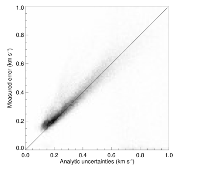
Figure 5.— A comparison of analytic uncertainties on the Doppler velocity measurements to the root mean square values of noise calculated from the data. The solid line highlights the line of gradient one to facilitate comparison.

4. Global properties of waves in the corona

Our interest lies in the temporal variation of the Doppler velocity and we will use relatively standard tools of analysis based around Fast Fourier Transforms (FFT). To begin with, periodograms are obtained for the typical velocity power spectrum for each of the boxed regions shown in Figure 1. To reduce spectral leakage in the frequency bins, initial processing steps are performed. First, the mean value of the Doppler velocity for the time-series is subtracted. This corresponds to suppressing the DC component of the time-series in the resulting power spectra. Next, the time-series is subject to apodisation with a Hann function.

Now, the following is applied to each boxed region. To find the average power in a region and its variance, the power from each time-series in a particular frequency bin is combined to provide a probability distribution function (PDF) for the velocity power at a certain frequency, from which a weighted sample mean, $\mu$, and the uncertainties on the estimate of the mean, $\sigma$, are obtained. The power in each frequency bin has a PDF that appears to be log-normal distributed. Hence, the mean and standard error of the distribution are calculated by binning the natural log of the power, where Poisson errors are used for weighting the calculation of the means that correspond to the uncertainties associated with the power binning. A linear function is fit to the means, weighted by the $\sigma$’s (Markwardt, 2009), in log-log space, such that when we transform back to velocity power this corresponds to a fit to the function $10^{a}f^{b}$, where $a$ and $b$ are determined from the fit parameters. The fit is performed in two separate regimes, for frequencies from 0.2-2.0 mHz and 4.1-11 mHz due to obvious presence of oscillatory power around $3$ mHz.

Before discussing the results, it is worth highlighting that the Doppler velocities from CoMP are a measure of the averaged value of velocities of many over-dense magnetic field lines contained within a single pixel. This naturally leads to smaller measured values for the Doppler velocities (De Moortel & Pascoe, 2012; McIntosh & De Pontieu, 2012). Hence, the magnitude of the power spectra measured here systematically underestimates the magnitude of the wave power and any other quantities estimated from the velocities. The number of unresolved magnetic field lines within a single pixel may play an important role in modifying the measurable Doppler velocity (McIntosh & De Pontieu, 2012). There is the possibility that the number of over-dense magnetic field lines will vary from active regions to open field regions/coronal holes, which could influence observed variations in the velocity amplitudes from region to region. However, we are not aware of any studies on the populations of magnetic structures, therefore, we assume that the differences in numbers are small, hence, the relative variations in the magnitudes of power spectra between the magnetically different regions are assumed to be predominantly due to differences in wave behaviour.

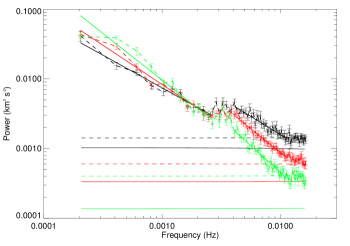
Figure 6.— The spatially averaged velocity power spectra. The black data points corresponds the open field region, the red data points are the quiet Sun region and the green data points are the active region. Each of the sets of data points are connected by a dashed line of the same colour. Over plotted are the fitted power law profiles (solid lines), with the values for the fits given in Table 1. The figure also shows estimates for the noise levels without seeing uncertainties (horizontal solid lines) and with them (horizontal dashed lines).

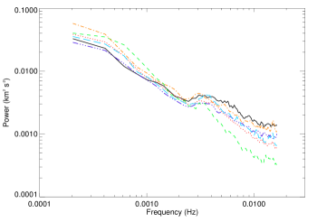
Figure 7.— The spatially averaged velocity power spectra including the additional regions. The figure is similar to that shown in Figure 6, where: black (solid) line OF; red (dot) line QS; green (dash) line AR; orange (dash-dot) line QS2; blue (long dash) line (QS3); purple (dash triple dot) line (QS4). Note the spectra have been smoothed with a 3-point box-car function for clarity. The variance and uncertainties for the QS2-4 features is comparable to those shown in Figure 6.

4.1. Average wave power in the corona

The calculated power spectra for three of the identified regions are shown in Figure 6 (AR, QS, OF) and all regions are shown in Figure 7. It is immediately clear that each power spectra has a slope that is $\propto f^{-b}$, i.e., dominated by an underlying power law spectrum, and that there are significant differences between the three spectra. The results of fitting the slopes (Table 1) elucidate these features, showing that the steepness of the slopes increases from the OF, to QS, to AR. The spectra demonstrate that for the the low frequencies, $f<2$ mHz, the power is initially greater in AR, with the OF and QS showing similar values for power (i.e., within 2-3 $\sigma$). The power spectra then converge around 1 mHz, with each spectrum showing a significant increase in power around 3 mHz. This enhancement of power provides a break in the $\propto f^{-b}$ trend, hence, is the reason we choose to break up the fitting of the spectra into two regimes. This increase in power around 3 mHz was previously identified in the large quiet Sun loops studied in Tomczyk & McIntosh (2009) and the open field region in Morton et al. (2015). These results suggest that this feature isn’t restricted to velocity fluctuations in certain magnetic geometries, but is prevalent through out the corona.

After the enhancement, as frequency continues to increase, the slope of the power spectra reverts back to that of a power law. Interestingly, the different regions show visibly different values for the velocity power at the high frequencies, with OF¿QS¿AR. As the velocity power is proportional to velocity amplitude, this indicates a difference in velocity amplitudes between the regions.

Below $\sim 100$ s, a knee appears in all the power spectra and they become almost flat. The simultaneity of the flattening suggests that this is due to noise dominating the power. The difference in the power of the noise between regions is likely partially due to the variation in emission between them, i.e. $\delta v(I)$. The lower intensities in open field regions and coronal holes compared to active regions, for example, means a lower signal to noise, hence, the magnitude of the errors in the estimated Doppler velocity increases. In turn, this leads to a higher noise level in the power spectra. This is confirmed by using the noise estimates to calculate the power of the noise for each spectra (Figure 6).

In Figure 7, the power spectra for all highlighted regions are shown. The plotted power spectra have been smoothed with a box-car filter of length three for aesthetic reasons only. The levels of the variance of the power for the additional quiet Sun regions are similar to that shown in the power spectra in Figure 6. It is found that the magnitude of the power spectra and also the spectral slopes of the additional regions are consistent with the previous quiet Sun measurements, somewhat bound between the open field and active region measurements.

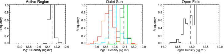
Figure 8.— Density measurements from the Fe XII line ratio. The middle panels displays the histograms for QS (black), QS2 (blue), QS3 (green) and QS4 (red). The distributions have been normalised with respect to the largest bin. The dashed lines in each panel mark the mean value of the density for each distribution.

4.2. Energy density

Now, we provide an assessment of the relative amount of wave energy stored in the different magnetic geometries by examining the wave energy density. The energy density is

$$\epsilon\propto\rho v^{2},$$

where $\rho$ is taken to be the average mass density of the local plasma. An estimate for the density can be obtained by utilising CoMP measurements of the Fe XIII emission lines at 10798 Å and 10747 Å, the ratio of which is sensitive to the electron number density, $n_{e}$ (Flower & Pineau des Forets, 1973). Using the CHIANTI database v7.0 (Landi et al., 2012), electron density versus intensity ratio curves are calculated for a range of heights above the photosphere taking into account the strong influence of photo-excitation on the formation of the two lines. The curves are then used to calculate the electron number density, which is converted to coronal mass density using $\rho=\mu m_{p}n_{e}$, where $\mu$ is the mean atomic weight (taken as 1.27 for coronal abundances) and $m_{p}$ is the proton mass.

In Figure 8 the distributions of measured density for each region are shown. The power spectra for each region is then multiplied by the corresponding mean density and displayed in Figure 9.

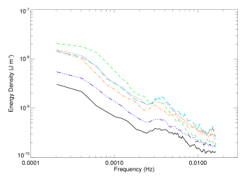
Figure 9.— The energy density spectra of the waves in different regions of the corona. The plotted spectra follow the same colour coding as described in Figure 7.

4.3. Energy Flux

Finally, we also estimate the flux of transverse wave energy through each of the regions. The energy flux is proportional to

$$F\propto\rho v^{2}c_{ph}=\epsilon c_{ph},$$

where $c_{ph}$ is the phase (or propagation) speed of the wave. An estimate of the propagation speeds of the observed waves can be obtained by cross-correlation of the Doppler velocity signals, full details of the process used are described in Tomczyk & McIntosh (2009) and Morton et al. (2015). The distributions of propagation speed measurements in each region are shown in Figure 10. The propagation speeds are significantly smaller in the active region, while the quiet Sun and open field regions display relatively similar values. It is likely that the angle between the magnetic structures that support the waves and the plane of sky will influence these results. The projection of the structure onto the plane of sky leads to a shorter apparent path taken by the wave, hence, measurement would give an underestimation of the propagation speed. This effect may be most influential on the active region measurements, with the AIA data indicating that the loops in the core of the active region are orientated with large angles to the plane of sky. Further, flows along the waveguides will also influence the measured speed of wave propagation. Bearing this in mind, the average value for the propagation speed in each region is determined and combined with the power spectra and density measurements to obtain an estimate for the energy flux for each region.

5. Discussion and conclusion

In the preceding section, time-series of velocity fluctuations in the corona between $1.05-1.3$ $R_{\odot}$ as observed with CoMP were examined. Average power spectra were obtained for various regions of the corona deemed as ‘typical’, in particular quiet Sun, active, and open field regions. The velocity fluctuations can be associated with transverse waves, most likely the swaying motions of coronal loops, i.e., kink waves. Additionally the energy density and energy flux of the waves are estimated. In the following, we discuss what inferences can be drawn from these measurements on the properties of kink waves in the corona.

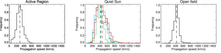
Figure 10.— Distribution of propagation speeds for each region. The middle panels displays the histograms for QS (black), QS2 (blue), QS3 (green) and QS4 (red). The distributions have been normalised with respect to the largest bin. The dashed lines in each panel mark the mean value of the phase speed for each distribution.

Table 1Measured properties of the different regions. The table displays the results of the $10^{a}f^{b}$ fit to the power spectra shown in Figure 6 in an open field region (OF), quiet Sun regions (QS, QS2, QS3, QS4) and active region (AR). Also given are the average density, $\rho$, and propagation speed, $c_{ph}$ for the regions and the standard deviations of the distributions.

	Frequency	a	b	$\chi^{2}_{\nu}$		$\rho$	$c_{ph}$
	Range (mHz)					(10-13 kg m-3)	(km s-1)
OF	0.2-2	$-4.9\pm 0.1$	$-0.94\pm 0.05$	1.3		0.9$\pm$0.4	420$\pm$80
	4-10	$-4.88\pm 0.1$	$-1.04\pm 0.06$	1.2
AR	0.2-2	$-6.0\pm 0.1$	$-1.34\pm 0.04$	6.3		5.1$\pm$0.7	290$\pm$90
	4-10	$-6.4\pm 0.1$	$-1.53\pm 0.06$	1.5
QS	0.2-2	$-5.5\pm 0.1$	$-1.13\pm 0.04$	1.79		4.0$\pm$0.5	420$\pm$120
	4-10	$-5.8\pm 0.1$	$-1.37\pm 0.04$	0.5
QS2	0.2-2	$-5.4\pm 0.1$	$-1.12\pm 0.05$	2.0		2.6$\pm$0.6	430$\pm$140
	4-10	$-4.8\pm 0.1$	$-0.98\pm 0.05$	1.4
QS3	0.2-2	$-5.4\pm 0.1$	$-1.09\pm 0.04$	2.1		4.1$\pm$0.6	400$\pm$80
	4-10	$-5.5\pm 0.1$	$-1.25\pm 0.05$	2.6
QS4	0.2-2	$-5.4\pm 0.1$	$-1.07\pm 0.04$	0.8		1.9$\pm$0.6	470$\pm$150
	4-10	$-4.8\pm 0.1$	$-0.95\pm 0.05$	1.1

5.1. The slope of the spectra

Each power spectrum measured here demonstrates power law behaviour (except for the enhancement around $3-5$ mHz), potentially indicating that the processes generating the coronal velocity power spectra are inherently stochastic in nature. This is perhaps hardly surprising considering that the magnetic fields are rooted in a turbulent photosphere, where the granulation is observed to buffet the magnetic flux concentrations (Berger & Title, 1996; van Ballegooijen et al., 1998; Keys et al., 2011; Chitta et al., 2012). The photospheric velocities imparted on the magnetic field can propagate into the corona via transverse waves, not before a significant fraction of the waves are reflected at the transition region, which will also play a role in determining the spectra of the motions that enter into the corona (e.g., Cranmer & van Ballegooijen, 2005; Verdini & Velli, 2007; van Ballegooijen et al., 2011).

What is also evident is that the slopes for each spectra show a relationship with magnetic geometry. As demonstrated in Morton et al. (2015), the power spectra derived for the open field region displays a $\sim 1/f$ slope, which is also observed in velocity fluctuations in the solar wind (Bavassano et al., 1982; Goldstein et al., 1995; Roberts, 2010). Further, although not shown, in this data set velocity fluctuations in other regions of the corona associated with a predominately open field have an approximately $1/f$ slope. The presence of the $1/f$ slope in the corona may provide support for the ideas presented in Verdini et al. (2012), who suggest that the spectra observed in the solar wind are already set in the low solar atmosphere, at least in the corona, and advected outwards.

The active region power spectra displays the steepest spectral slope with a gradient of $-1.5$, which may be indicative of the development of MHD turbulence in the closed coronal loops, particularly Iroshnikov-Kraichnan (IK) type turbulence. Modelling of Alfvén waves in closed coronal loops (e.g, van Ballegooijen et al., 2011) demonstrate that Alfvén waves injected in from both footpoints leads to counter-propagating wave packets that interact non-linearly and Alfvén wave turbulence develops and a heating of the coronal plasma ensues. Evidence for such counter propagating transverse waves has been observed previously with CoMP in large-scale quiescent loops (Tomczyk & McIntosh, 2009; De Moortel et al., 2014), as well as in an open field region (Morton et al., 2015). However, the slope of the power spectra of fluctuations expected from MHD turbulence is still uncertain, with arguments indicating it should be steeper than the $-1.5$ from IK theory (see, e.g., Bruno & Carbone, 2005; Petrosyan et al., 2010; for reviews on MHD turbulence).

The quiet Sun power spectra generally fall between these two ‘extreme’ slopes. This may reflect the fact that the quiet Sun regions analysed are composed a mixture of both open and closed field regions, as indicated by the SDO data (Figures 2 and 3 and from PFSS extrapolations), leading to an average spectral profile composed of both the open and closed magnetic field contributions. However, the QS4 region appears to contain predominantly closed field but its spectral slope is closer to $-1$, which may indicate other effects play a role in determining the quiet Sun spectral slopes.

5.2. Enhanced power at 3 mHz

The striking aspect of the spectra is that each one has an enhancement of power around 3 mHz (Fig. 7). A convincing theory to explain this feature is the mode conversion from p-modes to Alfvén waves close to transition region (as discussed in the introduction). As such, p-modes would play an important role in generating coronal transverse waves, injecting additional power at $3$ mHz that may the cascade to higher frequencies. The conversion of the global p-modes to transverse waves provides a natural explanation of how such an enhancement is coincident in all the power spectra from different regions.

Due to the enhancement being centred on 3 mHz, it may be tempting to attribute this feature to slow magneto-acoustic waves in the corona, driven by p-modes. However, it is known that slow waves are strongly damped at much lower heights in the corona than CoMP FOV covers. In particular, slow waves with periods around $\sim 3$ mHz above both polar regions (Gupta, 2014, Krishna Prasad et al., 2014) and active regions (De Moortel, 2009) appear to be killed off below 30” (1.03 $R_{\odot}$). Although, lower frequency ($<0.02$ mHz) slow waves are observed at larger heights ($>$1.06 $R_{\odot}$, e.g., Ofman et al., 1997, DeForest & Gurman, 1998, Banerjee et al., 2009, or for a review see Banerjee et al., 2011 and references within). Further, for slow waves in a coronal plasma, the perturbation of the plasma velocity is strictly parallel to the magnetic field orientation. To contribute to the measured power spectra, the slow waves would have to be propagating along magnetic fields parallel or inclined to the line-of-sight. This is odds with the close correlation between the measured direction of velocity signal propagation in the plane-of-sky and the magnetic field orientation (Tomczyk & McIntosh, 2009). Further, the typical measured propagation speeds are in excess of the estimated local sounds speed and no significant intensity oscillations seen with CoMP. As such, it is doubtful that slow waves contribute significantly the the measured velocity signal.

Alternatively, one could suggest that all observed transverse waves are excited in the photosphere by the horizontal motions of the convective photosphere and propagate into the corona. The results of the spectral evolution of Alfvén waves in Cranmer & van Ballegooijen (2005) demonstrate how an initial driving spectrum of photospheric horizontal motions could potentially lead to an enhancement in coronal power spectra due to the reflection at the transition region (e.g., Hollweg, 1978). However, it is unclear how active, quiescent and open field regions could produce such a similar enhancement of the spectra in this manner. First, photospheric flows are known to be suppressed in regions of increased magnetic flux density (Title et al., 1989). This would suggest driving spectra, and consequently the spectra of the generated transverse waves, would vary depending upon the density of magnetic flux, with evidence for this from chromospheric observations (Morton et al., 2014). Additionally, the magnetic and density scale heights are also likely to vary from region to region, meaning variations in the reflection/transmission profiles. The required combination of each of these factors in the different regions to produce a similar enhancement around 3 mHz appears unlikely.

5.3. Magnitude of the power

Qualitatively each of the power spectra derived for the different regions have similar characteristic features. However, there are distinct differences between the spectra (Figure 6 and 7). An apparent anti-correlation exists between the higher frequency power (2.5-10 mHz) and density, with power (hence, velocity amplitude) suppressed in the regions with the greatest density, i.e., the power (density) is least (greatest) in the active regions and greatest (least) in the open field regions (Table 1). Similar variations in amplitudes of oscillatory kink waves in the corona have been inferred from imaging observations with SDO (e.g., McIntosh et al., 2011). However, as mentioned, the larger spatial resolution of CoMP leads to an under-resolution of velocity amplitude and a direct comparison cannot be provided between the two sets of observations.

The lower frequency part of the power spectra displays different behaviour. There is no apparent correlation between the magnitude of the power in the higher frequency part of the spectrum and the low frequency part, although this could partially be due to uncertainties associated with the inherently small sampling of velocity amplitudes at the lower frequencies. At present it is unclear whether the power at these frequencies has an oscillatory component. Long period kink waves appear infrequent in SDO imaging data (e.g., Thurgood et al., 2014). The implication would be that oscillatory phenomenon do not contribute significantly to the magnitude of power spectra at the lower frequencies. However, this does not rule out the observed power is due to transverse waves. Waves do not have to be oscillatory in nature, for example they could be pulses. The power at lower frequencies may reflect some of the long term evolution the magnetic field undergoes and represent the magnitude of the signals that transmit the information about new states of coronal equilibrium (DeForest et al., 2014). For example, the recycling time of the coronal magnetic field is suggested to take place on time-scales of $\sim 1.4$ hours in the quiet Sun (Close et al., 2004).

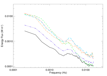
Figure 11.— The energy flux spectra of the waves in different regions of the corona. The plotted spectra follow the same colour coding as described in Figure 7.

5.4. Energy budgets

Finally, the wave energy density and flux for each region were estimated using density and propagation speed measurements from CoMP. It is found that for both quantities, the wave energy content across the corona is non-uniform. The energy density reveals that the wave energy stored in the quiet Sun magnetic structures is comparable to that of active regions, both of which exceed that of the polar open field region. This is not always the case though, for example the stored wave energy in the large-scale quiescent loops is comparable to the polar open field region.

The smaller values of the polar region energy density will be in part due to the largely one way propagation of waves and low densities. Morton et al. (2015) demonstrated the presence of counter-propagating transverse waves in open field regions, but the amplitude of the inward signals is smaller than the outward signals. In comparison, waves in closed structures appear to be excited at both footpoints, hence travel with comparable amplitudes in both directions.

Similar behaviour is also seen in the energy flux estimates. Although the open field region has larger values of propagation speeds compared to the active region (Fig 10, Table  1), the energy flux remains around a factor of two smaller for frequencies greater than $3$ mHz, increasing to a factor of 3 for lower frequencies.

Previous estimates of the coronal energy flux of kink waves have been provided from SDO observations (McIntosh et al., 2011; Thurgood et al., 2014). By the nature of the motions visible with SDO, those observations focus on waves with frequencies between $2-10$ mHz below heights of 1.05 $R_{\odot}$. The energy flux is calculated for an average value of velocity amplitude across the frequencies, however, the estimates imply the energy flux almost uniform throughout the corona. If we calculate the energy flux in a similar manner, we still find a non-uniform energy flux, with the active region energy flux one and half times greater than that estimated for the open field regions, and the quiet Sun around a factor of two greater.

It should be kept in mind that the number of structures contributing to CoMPs velocity signal may vary between the regions, potentially distorting the measure of velocity amplitude to a degree (McIntosh & De Pontieu, 2012). This would have some impact on the relative sizes of energy density and flux, but the number of structures would appear to need to vary by orders of magnitude to make an appreciable difference. Hence, we are confident that the measured differences in wave energy densities and fluxes are a physical feature of the corona.

5.5. Conclusion

Here, we have analysed the power spectra of velocity fluctuations in the corona in a variety of typical regions with different magnetic geometry. The fluctuations are thought to be associated with transverse waves (namely the kink mode), hence, the spectra give insight into the typical properties of these waves in the different regions. The results reveal the spectra are qualitatively the same throughout the corona, showing a steep spectral slope with a power enhancement around 3 mHz. However, there are distinctions between spectra (i.e., spectral slope; magnitudes of power, energy density, and energy flux), implying that the properties of the associated transverse waves vary in the different magnetic geometries. This is perhaps not surprising, and is broadly consistent with the impression from previous imaging observations.

The differing spectral slopes indicate variations in the underlying driving spectrum and evolution of the waves as they propagate through the lower solar atmosphere and corona. The measured slopes raise a number of questions, in particular, as to whether the $f^{-1.5}$ dependence in the active region is indicative of MHD turbulence and whether the quiet Sun slopes due to different phenomena or a mixture of contributions from features with $f^{-1.5}$ and $f^{-1}$ profiles.

As highlighted, each spectra shows evidence for a broad peak of enhanced power coincident at the same frequency range. This feature is present in all corona power spectra and indicates that there is a common driving mechanism operating on a global scale, that injects significant energy in to the corona around $3$ mHz. The source of the wave energy is potentially from the mode conversion of p-modes. Such a contribution is neglected in many Alfvén wave based heating models but the ubiquity of the feature throughout the corona would imply it plays a major role in determining the coronal wave energy budget.

Moreover, measures of the energy density and flux for each region were estimated, implying that significantly less energy flows through the open field region compared to quiet Sun regions and active regions. This is probably due to the largely one way flow of energy along open field lines (Morton et al., 2015), however, varying strengths of the wave driver and fraction of energy reflected at the Transition Region in each region will also play a role in determining the coronal energy flux of transverse waves.

Appendix A Estimating the seeing noise

In the main text (Section 3), an estimate for the seeing noise is given. Here we describe the method used to obtain the value.

Initially, the $\delta v$ for each pixel in each time frame is calculated from the contributions of photon, background and read noise. For each pixel, the uncertainty is then averaged over all time frames and the average uncertainty is used to generate a white noise time-series that is the same length as the data set. The power spectra of the noise is calculated for each pixel and averaged over the same spatial regions used for the velocity power spectra in Section 4.1. As to be expected, the resultant noise power spectra is approximately flat. The spectra are fit with a linear function and the results are shown as the solid horizontal lines in Figure 6. However, the estimated contribution of the uncertainties to the power is substantially less than the measured noise levels. To demonstrate this, the ratio of the power of the observed noise, $P_{M}$, to the expected power of the uncertainties, $P$, minus one, is shown in Figure 12. It can be clearly seen the level of underestimation varies between the regions, hence missing contribution is not a constant across the field of view.

The uncertainty (or noise) due to seeing conditions would have a dependence on the region under consideration due to the gradient of intensity differing between, say, an inhomogeneous active region and a more homogeneous coronal hole (see Eq. 6). In order to assess the affect of the seeing uncertainty, an estimate of $\sigma_{z}$ is needed.

In the following, we demonstrate that it is possible to estimate the value analytically using the ratio $P_{M}/P$. As inferred from Eq. (7), the error on velocity is given by,

$$\delta v^{2}=\left(\frac{\partial v}{\partial I_{1}}\delta I_{1}\right)^{2}+\left(\frac{\partial v}{\partial I_{2}}\delta I_{2}\right)^{2}+\left(\frac{\partial v}{\partial I_{3}}\delta I_{3}\right).$$ (A1)

The partial derivatives are independent of the uncertainties so they can be written as constants, e.g., $A,B,C$. Additionally, the assumption is made that the uncertainties on each of the original intensity measurements is similar, i.e., $\delta I_{1}\approx\delta I_{2}\approx\delta I_{3}$, hence, Eq. (A1) can be written

$$\delta v^{2}=(A+B+C)\delta I^{2}.$$ (A2)

Now, taking the ratio of the estimated noise in the power, $\propto\delta v^{2}$, and the measured noise in the power spectra, $\propto\delta v_{M}^{2}$ (with associated uncertainties $\delta I_{M}$), gives the following relation

$$\delta I_{M}^{2}=\delta I^{2}\frac{\delta v_{M}^{2}}{\delta v^{2}},$$ (A3)

where $\delta I^{2}$, ${\delta v_{M}^{2}}$ and ${\delta v^{2}}$ are known. The $\delta I_{M}$ has contributions from the same uncertainties as $\delta I$ plus the addition of the unaccounted for noise sources, which is assumed to be only the seeing noise at present. Then, writing the measured uncertainty in intensity as

$$\delta I_{M}^{2}=\delta I^{2}+\sigma_{seeing}^{2},$$ (A4)

and substituting into Eq. (A3) and rearranging gives

$$\sigma_{seeing}^{2}=\left(\frac{dI}{dz}\right)^{2}\sigma_{z}^{2}=\delta I^{2}\left(\frac{\delta v_{M}^{2}}{\delta v^{2}}-1\right).$$ (A5)

And finally, substituting in power for velocity squared we arrive at

$$\sigma_{seeing}^{2}=\left(\frac{dI}{dz}\right)^{2}\sigma_{z}^{2}=\delta I^{2}\left(\frac{P_{M}}{P}-1\right).$$ (A6)

Note, this equation only applies to the range of frequencies of the power spectra in Figure 6 in which the noise dominates. Lastly, an estimate of the gradient of the intensity for each pixel is required. To obtain this, a Sobel gradient operator is applied to an intensity image, which provides the magnitude gradient image (Gonzalez & Woods, 2002), as shown in Figure 13. It is clear that the intensity gradients are largest in the active region and least in the open field region. Now, using the noise dominated section of the velocity power spectra, i.e., from 10-16 mHz, an estimate for the $\sigma_{seeing}$ for each region is sought, and an average value of $0.1$ pixels is obtained. The corresponding uncertainty estimates demonstrate a much better agreement with the measured noise level (dashed horizontal lines in Figure 6).

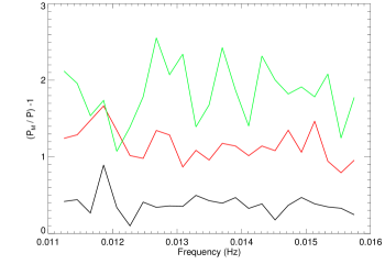
Figure 12.— The ratio of the expected noise level to the measured noise level for the velocity power spectra. The black line corresponds to the open field region, the red is the quiet Sun region and the green is the active region. The expected noise levels used here are determined excluding the influence of seeing jitter.

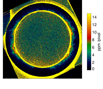
Figure 13.— Magnitude gradient image. An example of the gradient of the intensity calculated using a Sobel filter.

References

- Banerjee et al. (2011) Banerjee, D., Gupta, G. R., & Teriaca, L. 2011, Space Sci. Rev., 158, 267
- Banerjee et al. (2009) Banerjee, D., Teriaca, L., Gupta, G. R., et al. 2009, A&A, 499, L29
- Bavassano et al. (1982) Bavassano, B., Dobrowolny, M., Mariani, F., & Ness, N. F. 1982, J. Geophys. Res., 87, 3617
- Berger & Title (1996) Berger, T. E. & Title, A. M. 1996, ApJ, 463, 365
- Bethge et al. (2016) Bethge, C., Binay Karak, B., Tian, H., et al. 2016, In Prep
- Bogdan et al. (2003) Bogdan, T. J., Carlsson, M., Hansteen, V. H., et al. 2003, ApJ, 599, 626
- Brooks et al. (2013) Brooks, D. H., Warren, H. P., Ugarte-Urra, I., & Winebarger, A. R. 2013, ApJL, 772, L19
- Bruno & Carbone (2005) Bruno, R. & Carbone, V. 2005, Living Reviews in Solar Physics, 2, 4
- Cally (2011) Cally, P. S. 2011, in Astronomical Society of India Conference Series, Vol. 2, Astronomical Society of India Conference Series, 221–227
- Cally & Goossens (20008) Cally, P. S. & Goossens, M. 20008, Sol. Phys., 251, 251
- Cally & Hansen (2011) Cally, P. S. & Hansen, S. C. 2011, ApJ, 738, 119
- Chitta et al. (2012) Chitta, L. P., van Ballegooijen, A. A., Rouppe van der Voort, L., DeLuca, E. E., & Kariyappa, R. 2012, ApJ, 752, 48
- Close et al. (2004) Close, R. M., Parnell, C. E., Longcope, D. W., & Priest, E. R. 2004, ApJL, 612, L81
- Cranmer (2012) Cranmer, S. R. 2012, Space Sci. Rev., 172, 145
- Cranmer & van Ballegooijen (2005) Cranmer, S. R. & van Ballegooijen, A. A. 2005, ApJS, 156, 265
- De Moortel (2009) De Moortel, I. 2009, Space Science Reviews, 149, 65
- De Moortel et al. (2014) De Moortel, I., McIntosh, S. W., Threlfall, J., Bethge, C., & Liu, J. 2014, ApJ, 782, L34
- De Moortel & Pascoe (2012) De Moortel, I. & Pascoe, D. J. 2012, ApJ, 746, 31
- De Pontieu et al. (2004) De Pontieu, B., Erdélyi, R., & James, S. P. 2004, Nature, 430, 536
- De Pontieu et al. (2007a) De Pontieu, B., Hansteen, V. H., Rouppe van der Voort, L., van Noort, M., & Carlsson, M. 2007a, ApJ, 655, 624
- De Pontieu et al. (2007b) De Pontieu, B., McIntosh, S. W., Carlsson, M., et al. 2007b, Science, 318, 1574
- DeForest & Gurman (1998) DeForest, C. E. & Gurman, J. B. 1998, ApJL, 501, L217
- DeForest et al. (2014) DeForest, C. E., Howard, T. A., & McComas, D. J. 2014, ApJ, 787, 124
- Dowdy et al. (1986) Dowdy, Jr., J. F., Rabin, D., & Moore, R. L. 1986, Sol. Phys., 105, 35
- Edwin & Roberts (1983) Edwin, P. M. & Roberts, B. 1983, Sol. Phys., 88, 179
- Erdélyi & Ballai (2007) Erdélyi, R. & Ballai, I. 2007, Astronomische Nachrichten, 328, 726
- Erdélyi & Taroyan (2008) Erdélyi, R. & Taroyan, Y. 2008, A&A, 489, L49
- Fedun et al. (2009) Fedun, V., Erdélyi, R., & Shelyag, S. 2009, Sol. Phys., 258, 219
- Fedun et al. (2011) Fedun, V., Shelyag, S., & Erdélyi, R. 2011, ApJ, 727, 17
- Flower & Pineau des Forets (1973) Flower, D. R. & Pineau des Forets, G. 1973, A&A, 24, 181
- Gabriel (1976) Gabriel, A. H. 1976, Royal Society of London Philosophical Transactions Series A, 281, 339
- Gascoyne et al. (2014) Gascoyne, A., Jain, R., & Hindman, B. W. 2014, ApJ, 789, 109
- Goldstein et al. (1995) Goldstein, B. E., Smith, E. J., Balogh, A., et al. 1995, Geophys. Res. Lett., 22, 3393
- Gonzalez & Woods (2002) Gonzalez, R. C. & Woods, R. E. 2002, Digital image processing, 2nd edn. (Upper Saddle River, NJ: Prentice Hall)
- Goossens et al. (2009) Goossens, M., Terradas, J., Andries, J., Arregui, I., & Ballester, J. L. 2009, A&A, 503, 213
- Goossens et al. (2012) Goossens, M., Andries, Soler, R., Van Doorsselaere, T.,J., Arregui, I., & Terradas, J. 2012, ApJ, 753, 111
- Goossens et al. (2013) Goossens, M., Van Doorsselaere, T., Soler, R., & Verth, G. 2013, ApJ, 768, 191
- Gupta (2014) Gupta, G. R. 2014, A&A, 568, A96
- Hansen & Cally (2012) Hansen, S. C. & Cally, P. S. 2012, ApJ, 751, 31
- Hansteen & Velli (2012) Hansteen, V. H. & Velli, M. 2012, Space Sci. Rev., 172, 89
- He et al. (2009) He, J. S., Marsch, E., Tu, C., & Tian, H. 2009, ApJL, 705, L217
- Hillier et al. (2013) Hillier, A., Morton, R. J., & Erdélyi, R. 2013, ApJL, 779, L16
- Hollweg (1978) Hollweg, J. V. 1978, Sol. Phys., 56, 305
- Jain et al. (2011) Jain, R., Gascoyne, A., & Hindman, B. W. 2011, MNRAS, 415, 1276
- Jess et al. (2015) Jess, D. B., Morton, R. J., Verth, G., et al. 2015, Space Sci. Rev., 190, 103
- Keys et al. (2011) Keys, P. H., Mathioudakis, M., Jess, D. B., et al. 2011, ApJL, 740, L40
- Khomenko & Cally (2012) Khomenko, E. & Cally, P. S. 2012, ApJ, 746, 68
- Khomenko & Collados (2006) Khomenko, E. & Collados, M. 2006, ApJ, 653, 739
- Khomenko et al. (2008) Khomenko, E., Collados, M., & Felipe, T. 2008, Sol. Phys., 251, 589
- Klimchuk (2006) Klimchuk, J. A. 2006, Sol. Phys., 234, 41
- Krishna Prasad et al. (2014) Krishna Prasad, S., Banerjee, D., & Van Doorsselaere, T. 2014, ApJ, 789, 118
- Landi et al. (2012) Landi, E., Del Zanna, G., Young, P. R., Dere, K. P., & Mason, H. E. 2012, ApJ, 744, 99
- Lemen et al. (2012) Lemen, J. R., Title, A. M., Akin, D. J., et al. 2012, Sol. Phys., 275, 17
- Lilliefors (1969) Lilliefors, H. 1969, J AMER STATIST ASSN, 62, 399
- Markwardt (2009) Markwardt, C. B. 2009, in ASPCS, Vol. 411, Astronomical Data Analysis Software and Systems XVIII, ed. D. A. Bohlender, D. Durand, & P. Dowler, 251
- Matthaeus & Velli (2011) Matthaeus, W. H. & Velli, M. 2011, Space Sci. Rev., 160, 145
- McIntosh & De Pontieu (2012) McIntosh, S. W. & De Pontieu, B. 2012, ApJ, 761, 138
- McIntosh et al. (2011) McIntosh, S. W., de Pontieu, B., Carlsson, M., et al. 2011, Nature, 475, 477
- Morgan & Druckmüller (2014) Morgan, H. & Druckmüller, M. 2014, Sol. Phys., 289, 2945
- Morton & McLaughlin (2013) Morton, R. J. & McLaughlin, J. A. 2013, A&A, 553, 10
- Morton & McLaughlin (2014) Morton, R. J. & McLaughlin, J. A. 2014, ApJ, 789, 105
- Morton et al. (2015) Morton, R. J., Tomczyk, S., & Pinto, R. 2015, Nature Comms., 6, 7813
- Morton et al. (2013) Morton, R. J., Verth, G., Fedun, V., Shelyag, S., & Erdélyi, R. 2013, ApJ, 768, 17
- Morton et al. (2014) Morton, R. J., Verth, G., Hillier, A., & Erdélyi, R. 2014, ApJ, 784, 29
- Morton et al. (2012) Morton, R. J., Verth, G., Jess, D. B., et al. 2012, Nat. Commun., 3, 1315
- Narain & Ulmschneider (1996) Narain, U. & Ulmschneider, P. 1996, Space Sci. Rev., 75, 453
- Nisticò et al. (2013) Nisticò, G., Nakariakov, V. M., & Verwichte, E. 2013, A&A, 552, A57
- Ofman et al. (1997) Ofman, L., Romoli, M., Poletto, G., Noci, G., & Kohl, J. L. 1997, ApJL, 491, L111
- Okamoto et al. (2007) Okamoto, T. J., Tsuneta, S., Berger, T. E., et al. 2007, Science, 318, 1577
- Olsen (1993) Olsen, S. I. 1993, CVGIP: Graphical Models and Image Processing, 55, 319
- Osterbrock (1961) Osterbrock, D. E. 1961, ApJ, 134, 347
- Parnell & De Moortel (2012) Parnell, C. E. & De Moortel, I. 2012, Royal Society of London Philosophical Transactions Series A, 370, 3217
- Pereira et al. (2012) Pereira, T. M., De Pontieu, B., & Carlsson, M. 2012, ApJ, 759, 16
- Pesnell et al. (2012) Pesnell, W. D., Thompson, B. J., & Chamberlin, P. C. 2012, Sol. Phys., 275, 3
- Peter (2001) Peter, H. 2001, A&A, 374, 1108
- Petrosyan et al. (2010) Petrosyan, A., Balogh, A., Goldstein, M. L., et al. 2010, Space Sci. Rev., 156, 135
- Roberts (2010) Roberts, D. A. 2010, ApJ, 711, 1044
- Scherrer et al. (2012) Scherrer, P. H., Schou, J., Bush, R. I., et al. 2012, Sol. Phys., 275, 207
- Schrijver & De Rosa (2003) Schrijver, C. J. & De Rosa, M. L. 2003, Sol. Phys., 212, 165
- Schunker & Cally (2006) Schunker, H. & Cally, P. S. 2006, MNRAS, 372, 551
- Spruit (1982) Spruit, H. C. 1982, Sol. Phys., 75, 3
- Stangalini et al. (2013) Stangalini, M., Berrilli, F., & Consolini, G. 2013, A&A, 559, A88
- Stangalini et al. (2014) Stangalini, M., Consolini, G., Berrilli, F., De Michelis, P., & Tozzi, R. 2014, A&A, 569, A102
- Stangalini et al. (2015) Stangalini, M., Giannattasio, F., & Jafarzadeh, S. 2015, A&A, 577, A17
- Starck & Murtagh (2006) Starck, J.-L. & Murtagh, F. 2006, Astronomical Image and Data Analysis, 2nd edn. (Springer-Verlag Berlin Heidelberg)
- Threlfall et al. (2013) Threlfall, J., De Moortel, I., McIntosh, S. W., & Bethge, C. 2013, A&A, 556, A124
- Thurgood et al. (2014) Thurgood, J. O., Morton, R. J., & McLaughlin, J. A. 2014, ApJL, 790, L2
- Tian et al. (2013) Tian, H., Tomczyk, S., McIntosh, S. W., et al. 2013, Sol. Phys., 288, 637
- Title et al. (1989) Title, A. M., Tarbell, T. D., Topka, K. P., et al. 1989, ApJ, 336, 475
- Tomczyk et al. (2008) Tomczyk, S., Card, G. L., Darnell, T., et al. 2008, Sol. Phys., 247, 411
- Tomczyk & McIntosh (2009) Tomczyk, S. & McIntosh, S. W. 2009, ApJ, 697, 1384
- Tomczyk et al. (2007) Tomczyk, S., McIntosh, S. W., Keil, S. L., et al. 2007, Science, 317, 1192
- van Ballegooijen et al. (2011) van Ballegooijen, A. A., Asgari-Targhi, M., Cranmer, S. R., & DeLuca, E. E. 2011, ApJ, 736, 3
- van Ballegooijen et al. (1998) van Ballegooijen, A. A., Nisenson, P., Noyes, R. W., et al. 1998, ApJ, 509, 435
- Van Doorsselaere et al. (2014) Van Doorsselaere, T., Gijsen, S. E., Andries, J., & Verth, G. 2014, ApJ, 795, 18
- van Doorsselaere et al. (2008) van Doorsselaere, T., Nakariakov, V. M., Young, P. R., & Verwichte, E. 2008, A&A, 487, L17
- Verdini et al. (2012) Verdini, A., Grappin, R., Pinto, R., & Velli, M. 2012, ApJL, 750, L33
- Verdini & Velli (2007) Verdini, A. & Velli, M. 2007, ApJ, 662, 669
- Vigeesh et al. (2009) Vigeesh, G., Hasan, S. S., & Steiner, O. 2009, A&A, 508, 951
- Winebarger et al. (2014) Winebarger, A. R., Cirtain, J., Golub, L., et al. 2014, ApJL, 787, L10