Skewness of elliptic flow fluctuations

Abstract

Using event-by-event hydrodynamic calculations, we find that the fluctuations of the elliptic flow ($v_{2}$) in the reaction plane have a negative skew. We compare the skewness of $v_{2}$ fluctuations to that of initial eccentricity fluctuations. We show that skewness is the main effect lifting the degeneracy between higher-order cumulants, with negative skew corresponding to the hierarchy $v_{2}\{4\}>v_{2}\{6\}$ observed in Pb+Pb collisions at the CERN Large Hadron Collider. We describe how the skewness can be measured experimentally and show that hydrodynamics naturally reproduces its magnitude and centrality dependence.

I Introduction

Elliptic flow, $v_{2}$, is one of the key observables of ultrarelativistic heavy-ion collisions at BNL Relativistic Heavy Ion Collider Ackermann:2000tr and CERN Large Hadron Collider Aamodt:2010pa . Its large magnitude suggests that the strongly-coupled system formed in these collisions behaves collectively as a fluid Luzum:2008cw . However, quantitative comparison between hydrodynamic calculations and experimental data is hindered by the poor knowledge of the early collision dynamics and of the transport properties of the quark-gluon plasma Heinz:2013th . Therefore, it is essential to identify qualitative features predicted by hydrodynamics which can be tested against experimental data.

A crucial step in our understanding of collective motion has been the recognition that $v_{2}$ fluctuates event to event Miller:2003kd ; Alver:2006wh . Elliptic flow fluctuations are quantitatively probed by the cumulants Borghini:2001vi , $v_{2}\{k\}$, with $k=2,4,6,8$ Abelev:2014mda ; Aad:2014vba ; Khachatryan:2015waa . One typically observes $v_{2}\{2\}>v_{2}\{4\}$ and almost degenerate values for $v_{2}\{4\}$, $v_{2}\{6\}$, and $v_{2}\{8\}$, corresponding to Gaussian fluctuations of $v_{2}$ Voloshin:2007pc . A fine splitting (at the percent level) between $v_{2}\{4\}$ and $v_{2}\{6\}$ is, however, observed for most centralities Aad:2014vba . This splitting is a signature of non-Gaussian fluctuations Yan:2014nsa . Non-Gaussianity is in fact expected in hydrodynamics because $v_{2}$ is proportional to the corresponding spatial anisotropy (denoted by $\varepsilon_{2}$) of the initial density profile Gardim:2014tya , and the fluctuations of $\varepsilon_{2}$ present generic non-Gaussian properties Yan:2014afa ; Gronqvist:2016hym .

In this article, we identify the main source of non-Gaussian fluctuations with the skewness of elliptic flow fluctuations in the reaction plane. We compute the skewness in event-by-event hydrodynamics (Sec. II) and compare it with the skewness of eccentricity fluctuations. We then show (Sec. III), by means of an expansion in powers of the fluctuations, that skewness is the leading contribution to the fine structure of higher-order cumulants. We compare experimental data with hydrodynamic calculations. In Sec. IV, we derive a general formula relating the standardized skewness to the first three cumulants, $v_{2}\{2\}$, $v_{2}\{4\}$ and $v_{2}\{6\}$.

II Skewness in event-by-event hydrodynamics

In the flow picture Luzum:2011mm , particles are emitted independently in each collision with an azimuthal probability distribution, $P(\varphi)$, that fluctuates event to event. We choose a coordinate frame where $\varphi=0$ is the direction of the reaction plane. Elliptic flow is defined as the second Fourier coefficient of $P(\varphi)$, which has cosine and sine components:

$$v_{x} \equiv \frac{1}{2\pi}\int_{0}^{2\pi}P(\varphi)\cos 2\varphi\,d\varphi,$$ (1)

$$v_{y} \equiv \frac{1}{2\pi}\int_{0}^{2\pi}P(\varphi)\sin 2\varphi\,d\varphi.$$ (2)

Elliptic flow is a two-dimensional vector, ${\bf v}_{2}=v_{x}{\bf e}_{x}+v_{y}{\bf e}_{y}$. Using the standard terminology, we denote by $v_{2}$ the magnitude of ${\bf v}_{2}$, i.e. $v_{2}\equiv\sqrt{v_{x}^{2}+v_{y}^{2}}$.

Since the probability distribution, $P(\varphi)$, fluctuates event to event, the projections $v_{x}$ and $v_{y}$ are fluctuating quantities. In hydrodynamics, these fluctuations result mainly from the fluctuations of the initial energy density profile and are due to the probabilistic nature of the positions of the nucleons within nuclei at the time of impact Miller:2003kd ; Alver:2006wh . ${\bf v}_{2}$ is to a good approximation Gardim:2014tya ; Niemi:2012aj proportional to the initial eccentricity ${\boldsymbol{\varepsilon}}_{2}=(\varepsilon_{x},\varepsilon_{y})$, which is defined by Teaney:2010vd :

$$\varepsilon_{x} \equiv -\frac{\int\rho(r,\phi)r^{2}\cos 2\phi\,rdrd\phi}{\int\rho(r,\phi)r^{2}\,rdrd\phi},$$ (3)

$$\varepsilon_{y} \equiv -\frac{\int\rho(r,\phi)r^{2}\sin 2\phi\,rdrd\phi}{\int\rho(r,\phi)r^{2}\,rdrd\phi},$$ (4)

where $\rho(r,\phi)$ is the energy density deposited in the transverse plane shortly after the collision, in a centered polar coordinate system.

We model elliptic flow fluctuations by carrying out event-by-event hydrodynamic calculations of Pb+Pb collisions at 2.76 TeV, with initial conditions given by the Monte Carlo Glauber model Alver:2008aq ; Miller:2007ri ; Broniowski:2007nz . Our setup is the same as in Ref. Noronha-Hostler:2015dbi : The shear viscosity over entropy ratio is $\eta/s=0.08$ Policastro:2001yc within the viscous relativistic hydrodynamical code V-USPHYDRO Noronha-Hostler:2013gga ; Noronha-Hostler:2014dqa ; Noronha-Hostler:2015coa , which passes known analytical solutions Marrochio:2013wla , and $v_{x}$ and $v_{y}$ are calculated using Eq. (1) at freeze-out Teaney:2003kp for pions in the transverse momentum range $0.2<p_{t}<3$ GeV/$c$.

Figure 1: (Color online) Shaded areas: Histograms of the distribution of $v_{y}$ (a) and $v_{x}$ (b) for Pb+Pb collisions in the 50-55% centrality range. 5509 events were generated. Full lines: Histograms of the distributions of $\varepsilon_{y}$ (a) and $\varepsilon_{x}$ (b), rescaled by a response coefficient $\kappa=0.21$.

Figure 1 displays the histograms of the distributions of $v_{y}$ (a) and $v_{x}$ (b) in the 50-55% centrality bin. We choose this rather peripheral centrality range as an illustration because elliptic flow is close to its maximum value Aamodt:2010pa and presents large fluctuations. Values of $v_{x}$ are positive for most events, corresponding to elliptic flow in the reaction plane Ollitrault:1992bk . We denote by $\bar{v}_{2}$ its mean value

$$\bar{v}_{2}\equiv\langle v_{x}\rangle,$$ (5)

where angular brackets denote an average over events in a centrality class. Note that $\bar{v}_{2}$ is smaller than the mean elliptic flow, $\langle v_{2}\rangle=\langle\sqrt{v_{x}^{2}+v_{y}^{2}}\rangle$. The distribution of $v_{y}$ is centered at $0$ because parity conservation and symmetry with respect to the reaction plane imply that the probability distribution of $(v_{x},v_{y})$ is symmetric under $v_{y}\to-v_{y}$. The magnitude of the fluctuations is characterized by the variances of $v_{x}$ and $v_{y}$:

$$\sigma_{x}^{2} = \langle(v_{x}-\bar{v}_{2})^{2}\rangle=\langle v_{x}^{2}\rangle-\langle v_{x}\rangle^{2},$$ (6)

$$\sigma_{y}^{2} = \langle v_{y}^{2}\rangle.$$ (7)

For small fluctuations, the fluctuations of $v_{x}$ correspond to the fluctuations of the flow magnitude, while the fluctuations of $v_{y}$ correspond to the fluctuations of the flow angle. The so-called Bessel-Gaussian distribution Voloshin:2007pc of $v_{2}$ is obtained by assuming that the distribution of ${\bf v}_{2}$ is an isotropic two-dimensional Gaussian, i.e., $\sigma_{x}=\sigma_{y}$. While this is typically a good approximation for central and mid-central collisions, it becomes worse as the centrality percentile increases. In particular, Fig. 1 shows that $\sigma_{y}$ is slightly larger than $\sigma_{x}$, a general feature which can be traced back to the fluctuations of the initial eccentricity Yan:2014afa . The relative difference between $\sigma_{y}$ and $\sigma_{x}$ is in the fourth Fourier harmonic Ollitrault:1997di and, therefore, scales like $(\bar{v}_{2})^{2}$.

The distributions of $\varepsilon_{x}$ and $\varepsilon_{y}$ are also displayed in Fig. 1, rescaled by a coefficient $\kappa$, so that the mean value of $\varepsilon_{x}$ matches that of the $v_{x}$ distribution. If ${\bf v}_{2}$ was linearly proportional to ${\boldsymbol{\varepsilon}}_{2}$, then the two distributions would be identical. The distribution of $v_{x}$ is somewhat broader than that of $\varepsilon_{x}$, mostly because of a cubic response term, which is expected to have a sizable contribution at large centrality Noronha-Hostler:2015dbi .

One sees in Fig. 1 (b) that the distributions of $v_{x}$ and $\varepsilon_{x}$ are not symmetric with respect to their maximums: They present negative skew. The skewness of the distribution of $\varepsilon_{x}$ results from the condition $\varepsilon_{x}\leq 1$, which acts as a right cutoff Yan:2014afa . Skewness is typically characterized by the third moment of the fluctuations. The symmetry $v_{y}\to-v_{y}$ allows for two non trivial moments to order 3:

$$s_{1} \equiv \langle(v_{x}-\bar{v}_{2})^{3}\rangle,$$ (8)

$$s_{2} \equiv \langle(v_{x}-\bar{v}_{2})v_{y}^{2}\rangle.$$ (9)

The negative skew in Fig. 1 (b) corresponds to $s_{1}<0$. For dimensional reasons, a standardized skewness is usually employed, which is defined as

$$\gamma_{1}\equiv\frac{s_{1}}{\sigma_{x}^{3}}.$$ (10)

Figure 2: (Color online) Standardized skewness of elliptic flow fluctuations (open circles) and of initial eccentricity fluctuations (full circles) from hydrodynamic calculations, as a function of centrality percentile, for Pb+Pb collisions at 2.76 TeV. Symbols have been slightly shifted horizontally for the sake of readability. The shaded band displays the value of $\gamma_{1}$ estimated from the cumulants of $v_{2}$, as defined by Eq. (25).

Figure 2 displays the standardized skewness, $\gamma_{1}$, calculated in hydrodynamics as a function of the collision centrality. It is negative above $15\%$ centrality and its absolute magnitude increases as a function of centrality percentile. This increase results from two effects: First, $\gamma_{1}$ vanishes by symmetry for central collisions and is typically proportional to $\bar{v}_{2}$; second, it is a first-order correction to the central limit and is, therefore, inversely proportional to the square root of the system size Gronqvist:2016hym . Figure 2 also displays the standardized skewness of the $\varepsilon_{x}$ fluctuations, which, as we pointed out before, would be identical to that of the $v_{x}$ fluctuations if ${\bf v}_{2}$ were exactly linearly proportional to ${\boldsymbol{\varepsilon}}_{2}$. We observe that the standardized skewness calculated from ${\bf v}_{2}$ becomes smaller in absolute value than the initial skewness calculated from ${\boldsymbol{\varepsilon}}_{2}$ as the centrality percentile increases. Hence, the hydrodynamical evolution washes out part of the initial skewness. This effect, which is clearly seen in the histogram of Fig. 1, is mostly due to the cubic response of the system, which increases $\sigma_{x}$ Noronha-Hostler:2015dbi .

Equations (5)–(8) are the first-order terms in a cumulant expansion of the flow fluctuations. The formalism of generating functions provides a compact formulation for the cumulant expansion. The Fourier-Laplace transform of the distribution of ${\bf v_{2}}$ is $\langle e^{{\bf k}\cdot{\bf v}_{2}}\rangle$, where ${\bf k}\equiv k_{x}{\bf e}_{x}+k_{y}{\bf e}_{y}$ is a two-dimensional vector. The generating function of the cumulants is its logarithm, $\ln\langle e^{{\bf k}\cdot{\bf v}_{2}}\rangle$. By expanding it up to order 3 in ${\bf k}$, one obtains

$$\ln\langle e^{{\bf k}\cdot{\bf v}_{2}}\rangle=k_{x}\bar{v}_{2}+\frac{k_{x}^{2}}{2}\sigma_{x}^{2}+\frac{k_{y}^{2}}{2}\sigma_{y}^{2}+\frac{k_{x}^{3}}{6}s_{1}+\frac{k_{x}k_{y}^{2}}{2}s_{2},$$ (11)

where $\bar{v}_{2}$, $\sigma_{x}$, $\sigma_{y}$, $s_{1}$, and $s_{2}$ are given by Eqs. (5)–(8).

III The fine structure of higher-order cumulants

The direction of the reaction plane is not known experimentally. Therefore, the skewness of the $v_{x}$ fluctuations defined in Eq. (10) cannot be measured directly. More specifically, there is no simple way of extracting it from the probability distribution of the flow magnitude, $v_{2}$ Aad:2013xma . In this section, we show how one can relate the skewness to quantities which are measured experimentally, specifically, the cumulants of the distribution of $v_{2}$.

Experimental observables are measured in the laboratory frame where the orientation of the reaction plane has a flat distribution. The cumulants of the distribution of $v_{2}$, as measured in experiments Aamodt:2010pa ; Aad:2014vba ; Adler:2002pu ; Alt:2003ab ; Chatrchyan:2012ta , are defined in this frame Borghini:2000sa ; Borghini:2001vi . Their generating function is given by the left-hand side of Eq. (11), with the only difference that one averages over the orientation of the reaction plane before taking the logarithm: One exponentiates Eq. (11), substitutes $k_{x}=k\cos\varphi$ and $k_{y}=k\sin\varphi$, averages over $\varphi$, and finally takes the logarithm:

$$\ln G(k)\equiv\ln\left(\int_{0}^{2\pi}\frac{d\varphi}{2\pi}\langle\textup{e}^{{\bf k}\cdot{\bf v}_{2}}\rangle\right).$$ (12)

The $2n$-th order cumulant, $v_{2}\{2n\}$, is eventually given by the $2n$-th order term of the Taylor expansion of $\ln G({k})$ computed at $k=0$. More specifically Borghini:2001vi :

$$\left.\frac{d^{2n}}{dk^{2n}}\ln I_{0}(kv_{2}\{2n\})\right|_{k=0}\equiv\left.\frac{d^{2n}}{dk^{2n}}\ln G(k)\right|_{k=0}.$$ (13)

In the simple case of Bessel-Gaussian fluctuations, $s_{1}=s_{2}=0$ and $\sigma_{y}=\sigma_{x}$. Inserting Eq. (11) into Eq. (12), one obtains

$$\ln G(k)=\ln I_{0}(k\bar{v}_{2})+\frac{k^{2}\sigma_{x}^{2}}{2},$$ (14)

and Eq. (13) yields

$$v_{2}\{2\} = \sqrt{(\bar{v}_{2})^{2}+2\sigma_{x}^{2}},$$ (15)

$$v_{2}\{4\}=v_{2}\{6\}=\cdots = \bar{v}_{2}.$$ (16)

Therefore, the cumulants of order $n\geq 4$ are identical to the mean elliptic flow in the reaction plane Voloshin:2007pc .

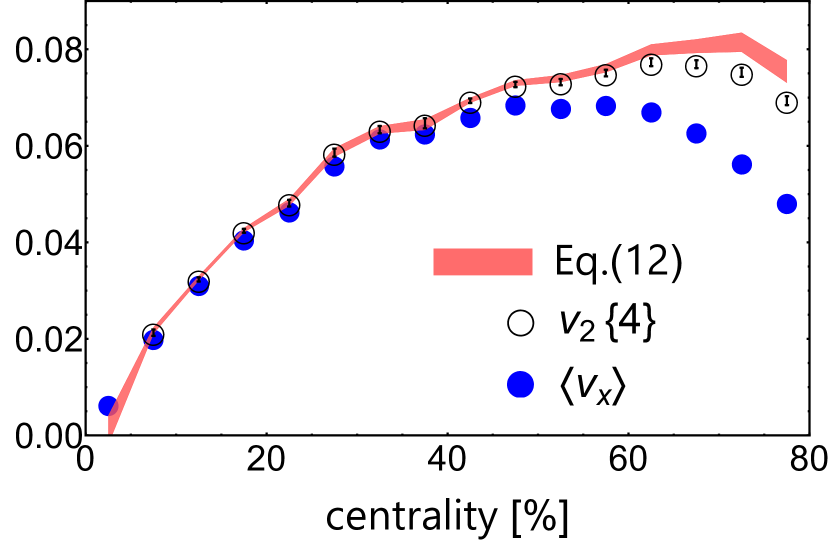
Figure 3: (Color online) Open symbols: $v_{2}\{4\}$ vs centrality in event-by-event hydrodynamics. Full symbols: mean elliptic flow in the reaction plane $\langle v_{x}\rangle=\bar{v}_{2}$. Shaded band: right-hand side of Eq. (17) for $v_{2}\{4\}$, corresponding to the leading non-Gaussian corrections.

In event-by-event hydrodynamics, the direction of the reaction plane is known and one can compute both $v_{2}\{4\}$ Qiu:2011iv ; Hirano:2012kj ; Bozek:2013uha ; Niemi:2015qia and $\bar{v}_{2}$. Figure 3 shows their dependence on the centrality percentile. They are compatible up to $40\%$ centrality. For peripheral collisions, $v_{2}\{4\}$ becomes significantly larger than $\bar{v}_{2}$, which means that the Bessel-Gaussian ansatz fails Qiu:2011iv . This failure can be attributed either to the asymmetry of the fluctuations, $\sigma_{x}\not=\sigma_{y}$, or to non-Gaussian fluctuations. Both these features are expected in hydrodynamics, as shown in Sec. II. Expanding the generating function in powers of the fluctuations and keeping only the leading order terms in $\sigma_{y}^{2}-\sigma_{x}^{2}$, $s_{1}$ and $s_{2}$, we obtain:

$$v_{2}\{2\} = \sqrt{(\bar{v}_{2})^{2}+\sigma_{x}^{2}+\sigma_{y}^{2}},$$ (17)

$$v_{2}\{4\} \simeq \bar{v}_{2}+\frac{\sigma_{y}^{2}-\sigma_{x}^{2}}{2\bar{v}_{2}}-\frac{s_{1}+s_{2}}{(\bar{v}_{2})^{2}},$$ (18)

$$v_{2}\{6\} \simeq \bar{v}_{2}+\frac{\sigma_{y}^{2}-\sigma_{x}^{2}}{2\bar{v}_{2}}-\frac{\frac{2}{3}s_{1}+s_{2}}{(\bar{v}_{2})^{2}},$$ (19)

$$v_{2}\{8\} \simeq \bar{v}_{2}+\frac{\sigma_{y}^{2}-\sigma_{x}^{2}}{2\bar{v}_{2}}-\frac{\frac{7}{11}s_{1}+s_{2}}{(\bar{v}_{2})^{2}},$$ (20)

When these corrections are added, higher-order cumulants are no longer equal to $\bar{v}_{2}$. The shaded band in Fig. 3 corresponds to the right-hand side of the second line of Eq. (17), where all terms are calculated in hydrodynamics. Agreement with the left-hand side is excellent for all centralities. The term proportional to the asymmetry of the fluctuations, $\sigma_{y}^{2}-\sigma_{x}^{2}$, turns out to be negligible: The leading correction is the term proportional to $s_{1}+s_{2}$, due to the non-Gaussianity of the fluctuations.

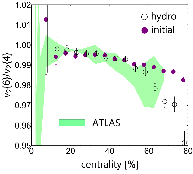
Figure 4: (Color online) Shaded band: ATLAS data for $v_{2}\{6\}/v_{2}\{4\}$ versus centrality Aad:2013xma . Error bars take into account the strong correlation between $v_{2}\{6\}$ and $v_{2}\{4\}$ Borghini:2001vi . Open symbols: hydrodynamic calculations. Full symbols: $\varepsilon_{2}\{6\}/\varepsilon_{2}\{4\}$.

Non-Gaussian fluctuations not only increase the value of $v_{2}\{4\}$: They also induce a splitting between $v_{2}\{4\}$, $v_{2}\{6\}$ and $v_{2}\{8\}$. Subtracting the second and third line of Eq. (17), one obtains:

$$v_{2}\{4\}-v_{2}\{6\}=-\frac{s_{1}}{3(\bar{v}_{2})^{2}}.$$ (21)

The splitting is solely due to the coefficient $s_{1}$, corresponding to the skewness of elliptic flow fluctuations in the reaction plane. Figure 4 displays ATLAS data for $v_{2}\{6\}/v_{2}\{4\}$ versus centrality for Pb+Pb collisions at 2.76 TeV. We use the data from Fig. 9b of Ref. Aad:2014vba , inferred from the event-by-event distribution of $v_{2}$ Aad:2013xma , which have smaller error bars than the direct cumulant measurements. $v_{2}\{4\}$ and $v_{2}\{6\}$ are very close to one another, but one observes a fine structure, at the percent level, for most centralities: $v_{2}\{4\}$ is larger than $v_{2}\{6\}$. This, according to Eq. (21), implies $s_{1}<0$, in line with our expectation from the hydrodynamic calculations presented in Sec. II. We carry out a more quantitative comparison by numerical calculations of $v_{2}\{6\}/v_{2}\{4\}$ in hydrodynamics. The result is displayed in Fig. 4 (open symbols). It is compatible with experimental data within error bars. Precise figures depend on the model of initial conditions, but Fig. 4 shows that hydrodynamics naturally captures the skewness of the $v_{2}$ fluctuations, hence the splitting between $v_{2}\{4\}$ and $v_{2}\{6\}$.

In our hydrodynamic calculation, the ratio $v_{2}\{6\}/v_{2}\{4\}$ coincides with the corresponding ratio for initial eccentricities, $\varepsilon_{2}\{6\}/\varepsilon_{2}\{4\}$, up to 60% centrality. We stress that this was not a priori expected because the cubic response breaks simple proportionality and decreases the skewness of the distribution of $v_{2}$ compared to that of $\varepsilon_{2}$. While the cubic response has an important effect on the ratio $v_{2}\{4\}/v_{2}\{2\}$ Noronha-Hostler:2015dbi , it does not seem to affect the ratio $v_{2}\{6\}/v_{2}\{4\}$, which directly reflects the ratio $\varepsilon_{2}\{6\}/\varepsilon_{2}\{4\}$ provided by the model of initial conditions.

Equation (17) also gives the following universal prediction for the small splitting between $v_{2}\{6\}$ and $v_{2}\{8\}$:

$$v_{2}\{6\}-v_{2}\{8\}=\frac{1}{11}(v_{2}\{4\}-v_{2}\{6\}).$$ (22)

The number of events in our hydrodynamic calculation is too small to test this relation. However, the same relation can be written for the cumulants of the initial eccentricity, $\varepsilon_{2}$. It is obtained by replacing $v_{2}$ with $\varepsilon_{2}$ everywhere in the derivation, and thus does not involve any relation between $\varepsilon_{2}$ and $v_{2}$. We have tested Eq. (22) for the fluctuations of $\varepsilon_{2}$ within a Monte Carlo Glauber model, which allows for much higher statistics than full hydrodynamic calculations. We find that Eq. (22) is approximately satisfied for central collisions, but that the left-hand side becomes larger than the right-hand side as the centrality percentile increases. This means that the expansion leading to Eq. (22) is unable to capture accurately the splitting between $\varepsilon_{2}\{6\}$ and $\varepsilon_{2}\{8\}$, and consequently the splitting between $v_{2}\{6\}$ and $v_{2}\{8\}$.

IV Measuring the skewness with cumulants

In this section we explain how to estimate the standardized skewness, $\gamma_{1}$, defined in Eq. (10), from $v_{2}\{2\}$, $v_{2}\{4\}$, and $v_{2}\{6\}$. We estimate $s_{1}$ using Eq. (21). Since this result is derived from a perturbative expansion to first order in $s_{1}$, we estimate also $\gamma_{1}$ to first order. By doing so, we neglect small non-Gaussian contributions to $\bar{v}_{2}$ and $\sigma_{x}$: We use the Gaussian approximation, Eq. (15), which gives

$$v_{2}\{4\} = \bar{v}_{2},$$ (23)

$$v_{2}\{2\}^{2}-v_{2}\{4\}^{2} = 2\sigma_{x}^{2}.$$ (24)

Using Eqs. (21) and (23), we obtain the following estimate of $\gamma_{1}$, which we denote by $\gamma_{1}^{\rm expt}$:

$$\gamma_{1}^{\rm expt}\equiv-6\sqrt{2}\,v_{2}\{4\}^{2}\frac{v_{2}\{4\}-v_{2}\{6\}}{(v_{2}\{2\}^{2}-v_{2}\{4\}^{2})^{3/2}}.$$ (25)

Figure 5: (Color online) Contour plot of the difference $\gamma_{1}^{\rm expt}~{}-~{}\gamma_{1}$, with $\gamma_{1}^{\rm expt}$ defined in Eq. (25) and $\gamma_{1}$ defined in Eq. (10), computed by means of the elliptic-power distribution Yan:2014afa , in the $(\alpha,\varepsilon_{0})$ parameter plane. Squares correspond to the values of $\alpha$ and $\varepsilon_{0}$ extracted from Monte Carlo Glauber Alver:2008aq simulations of Pb+Pb collisions at 2.76 TeV, which are fitted to the elliptic-power distribution.

We check the accuracy of $\gamma_{1}^{\rm expt}$ as an estimate of $\gamma_{1}$ using two different methods. The first method is to compute both $\gamma_{1}$ and $\gamma_{1}^{\textup{expt}}$ in event-by-event hydrodynamics. $\gamma_{1}^{\rm expt}$ is shown as a shaded band in Fig. 2. It is in good agreement with $\gamma_{1}$ up to 60% centrality. Above 60% centrality, the approximation $v_{2}\{4\}\simeq\bar{v}_{2}$ breaks down, as shown by Fig. 3. Statistical errors in our hydrodynamic calculation are significant due to the limited amount of events in each centrality bin. Therefore we employ a second method. Since Eq. (25) can be derived as well for the skewness of the distribution of $\varepsilon_{2}$, we test the validity of this relation using the elliptic-power distribution Yan:2014afa , which is a simple analytical model for the distribution of $(\varepsilon_{x},\varepsilon_{y})$. The elliptic-power distribution has two parameters: $\varepsilon_{0}$, which approximately gives the mean eccentricity in the reaction plane, $\varepsilon_{0}\simeq\langle\varepsilon_{x}\rangle$, and $\alpha$, which is proportional to the number of participants. We evaluate both $\gamma_{1}$ and $\gamma_{1}^{\rm expt}$ as a function of $\varepsilon_{0}$ and $\alpha$. Fluctuations scale like $1/\sqrt{\alpha}$, therefore, the assumption of small fluctuations made in deriving Eq. (17) holds for $\alpha\gg 1$. One also expects approximations to break down in the limit $\varepsilon_{0}\to 0$ (corresponding to the limiting case of the power distribution Yan:2013laa ) where $\gamma_{1}$ vanishes by symmetry while $\gamma_{1}^{\rm expt}$ does not. Figure 5 indeed shows that the difference between the estimated skewness and the true skewness is large only when both $\alpha$ and $\varepsilon_{0}$ are small. In order to estimate the range of $\alpha$ and $\varepsilon_{0}$ applicable to Pb+Pb collisions, we perform Monte Carlo Glauber Alver:2008aq simulations and fit the resulting distribution of $\varepsilon_{2}$ to the elliptic-power distribution, for different centrality windows. The values of $\alpha$ and $\varepsilon_{0}$ extracted from the fits are shown as squares in Fig. 5. Based on this figure, and since in hydrodynamics the skewness of $v_{2}$ is comparable to that of $\varepsilon_{2}$, we expect the difference $|\gamma_{1}^{\rm expt}-\gamma_{1}|$ to be a few $10^{-2}$ for Pb+Pb collisions, much smaller in absolute value than the value of $\gamma_{1}$ in Fig. 2. Therefore, Eq. (25) should provide a reasonable estimate of the standardized skewness also from experimental data.

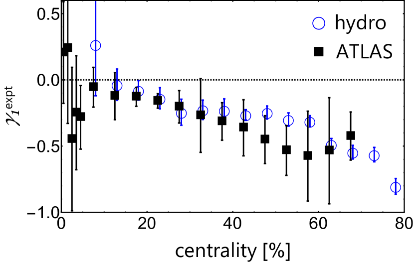
Figure 6: (Color online) Standardized skewness of $v_{2}$ fluctuations, as defined in Eq. (25), as a function of centrality. Squares: ATLAS data. Circles: hydrodynamic calculations, corresponding to the dark shaded band in Fig. 2. Symbols have been slightly shifted horizontally for the sake of readability.

Figure 6 displays the skewness extracted from ATLAS data Aad:2013xma using Eq. (25). The standardized skewness is moderate but not small, and reaches $-0.5$ in peripheral collisions, although with large error bars. Errors have been estimated by adding statistical and systematic errors in quadrature, and assuming that the errors on $v_{2}\{2\}$, $v_{2}\{4\}$, and $v_{2}\{6\}/v_{2}\{4\}$ are uncorrelated. Since errors on $v_{2}\{2\}$ and $v_{2}\{4\}$ are usually correlated, the errors on ATLAS data in Fig. 6 are probably overestimated. Hydrodynamic calculations are compatible with experimental data in the full range of centrality.

V Conclusions

We have shown that the small splitting of higher-order cumulants of the elliptic flow from mid-central up to peripheral ultrarelativistic nucleus-nucleus collisions is mostly due to the skewness of the fluctuations of the elliptic flow in the reaction plane, $v_{x}$. We emphasize that this is a general result which does not depend on any particular model. Negative skewness is observed in Pb+Pb data, and is naturally explained in hydrodynamics: it follows from the fact that $v_{2}$ is approximately proportional to the initial eccentricity, and that the eccentricity in the reaction plane is bounded by unity. The splitting between $v_{2}\{4\}$ and $v_{2}\{6\}$ thus provides additional evidence of the collective origin of elliptic flow. We have computed the ratio $v_{2}\{6\}/v_{2}\{4\}$ in event-by-event viscous hydrodynamics and we have shown that it is very close to the ratio $\varepsilon_{2}\{6\}/\varepsilon_{2}\{4\}$ between the cumulants of the initial eccentricity. Thus, this observable constrains the early dynamics of the quark-gluon plasma Hirano:2005xf ; Bhalerao:2011yg ; Schenke:2012wb ; Albacete:2013tpa ; Renk:2014jja .

References

- (1) K. H. Ackermann et al. [STAR Collaboration], Phys. Rev. Lett. 86, 402 (2001) doi:10.1103/PhysRevLett.86.402 [nucl-ex/0009011].
- (2) K. Aamodt et al. [ALICE Collaboration], Phys. Rev. Lett. 105, 252302 (2010) doi:10.1103/PhysRevLett.105.252302 [arXiv:1011.3914 [nucl-ex]].
- (3) M. Luzum and P. Romatschke, Phys. Rev. C 78, 034915 (2008) Erratum: [Phys. Rev. C 79, 039903 (2009)] doi:10.1103/PhysRevC.78.034915, 10.1103/PhysRevC.79.039903 [arXiv:0804.4015 [nucl-th]].
- (4) U. Heinz and R. Snellings, Ann. Rev. Nucl. Part. Sci. 63, 123 (2013) doi:10.1146/annurev-nucl-102212-170540 [arXiv:1301.2826 [nucl-th]].
- (5) M. Miller and R. Snellings, nucl-ex/0312008.
- (6) B. Alver et al. [PHOBOS Collaboration], Phys. Rev. Lett. 98, 242302 (2007) doi:10.1103/PhysRevLett.98.242302 [nucl-ex/0610037].
- (7) N. Borghini, P. M. Dinh and J. Y. Ollitrault, Phys. Rev. C 64, 054901 (2001) doi:10.1103/PhysRevC.64.054901 [nucl-th/0105040].
- (8) B. B. Abelev et al. [ALICE Collaboration], Phys. Rev. C 90, no. 5, 054901 (2014) doi:10.1103/PhysRevC.90.054901 [arXiv:1406.2474 [nucl-ex]].
- (9) G. Aad et al. [ATLAS Collaboration], Eur. Phys. J. C 74, no. 11, 3157 (2014) doi:10.1140/epjc/s10052-014-3157-z [arXiv:1408.4342 [hep-ex]].
- (10) V. Khachatryan et al. [CMS Collaboration], Phys. Rev. Lett. 115, no. 1, 012301 (2015) doi:10.1103/PhysRevLett.115.012301 [arXiv:1502.05382 [nucl-ex]].
- (11) S. A. Voloshin, A. M. Poskanzer, A. Tang and G. Wang, Phys. Lett. B 659, 537 (2008) doi:10.1016/j.physletb.2007.11.043 [arXiv:0708.0800 [nucl-th]].
- (12) L. Yan, J. Y. Ollitrault and A. M. Poskanzer, Phys. Lett. B 742, 290 (2015) doi:10.1016/j.physletb.2015.01.039 [arXiv:1408.0921 [nucl-th]].
- (13) F. G. Gardim, J. Noronha-Hostler, M. Luzum and F. Grassi, Phys. Rev. C 91, no. 3, 034902 (2015) doi:10.1103/PhysRevC.91.034902 [arXiv:1411.2574 [nucl-th]].
- (14) L. Yan, J. Y. Ollitrault and A. M. Poskanzer, Phys. Rev. C 90, no. 2, 024903 (2014) doi:10.1103/PhysRevC.90.024903 [arXiv:1405.6595 [nucl-th]].
- (15) H. Grönqvist, J. P. Blaizot and J. Y. Ollitrault, Phys. Rev. C 94, no. 3, 034905 (2016) doi:10.1103/PhysRevC.94.034905 [arXiv:1604.07230 [nucl-th]].
- (16) M. Luzum, J. Phys. G 38, 124026 (2011) doi:10.1088/0954-3899/38/12/124026 [arXiv:1107.0592 [nucl-th]].
- (17) H. Niemi, G. S. Denicol, H. Holopainen and P. Huovinen, Phys. Rev. C 87, no. 5, 054901 (2013) doi:10.1103/PhysRevC.87.054901 [arXiv:1212.1008 [nucl-th]].
- (18) D. Teaney and L. Yan, Phys. Rev. C 83, 064904 (2011) doi:10.1103/PhysRevC.83.064904 [arXiv:1010.1876 [nucl-th]].
- (19) B. Alver, M. Baker, C. Loizides and P. Steinberg, arXiv:0805.4411 [nucl-ex].
- (20) M. L. Miller, K. Reygers, S. J. Sanders and P. Steinberg, Ann. Rev. Nucl. Part. Sci. 57, 205 (2007) doi:10.1146/annurev.nucl.57.090506.123020 [nucl-ex/0701025].
- (21) W. Broniowski, M. Rybczynski and P. Bozek, Comput. Phys. Commun. 180, 69 (2009) doi:10.1016/j.cpc.2008.07.016 [arXiv:0710.5731 [nucl-th]].
- (22) J. Noronha-Hostler, L. Yan, F. G. Gardim and J. Y. Ollitrault, Phys. Rev. C 93, no. 1, 014909 (2016) doi:10.1103/PhysRevC.93.014909 [arXiv:1511.03896 [nucl-th]].
- (23) G. Policastro, D. T. Son and A. O. Starinets, Phys. Rev. Lett. 87, 081601 (2001) doi:10.1103/PhysRevLett.87.081601 [hep-th/0104066].
- (24) J. Noronha-Hostler, G. S. Denicol, J. Noronha, R. P. G. Andrade and F. Grassi, Phys. Rev. C 88, no. 4, 044916 (2013) doi:10.1103/PhysRevC.88.044916 [arXiv:1305.1981 [nucl-th]].
- (25) J. Noronha-Hostler, J. Noronha and F. Grassi, Phys. Rev. C 90, no. 3, 034907 (2014) doi:10.1103/PhysRevC.90.034907 [arXiv:1406.3333 [nucl-th]].
- (26) J. Noronha-Hostler, J. Noronha and M. Gyulassy, Phys. Rev. C 93, no. 2, 024909 (2016) doi:10.1103/PhysRevC.93.024909 [arXiv:1508.02455 [nucl-th]].
- (27) H. Marrochio, J. Noronha, G. S. Denicol, M. Luzum, S. Jeon and C. Gale, Phys. Rev. C 91, no. 1, 014903 (2015) doi:10.1103/PhysRevC.91.014903 [arXiv:1307.6130 [nucl-th]].
- (28) D. Teaney, Phys. Rev. C 68, 034913 (2003) doi:10.1103/PhysRevC.68.034913 [nucl-th/0301099].
- (29) J. Y. Ollitrault, Phys. Rev. D 46, 229 (1992). doi:10.1103/PhysRevD.46.229
- (30) J. Y. Ollitrault, nucl-ex/9711003.
- (31) G. Aad et al. [ATLAS Collaboration], JHEP 1311, 183 (2013) doi:10.1007/JHEP11(2013)183 [arXiv:1305.2942 [hep-ex]].
- (32) C. Adler et al. [STAR Collaboration], Phys. Rev. C 66, 034904 (2002) doi:10.1103/PhysRevC.66.034904 [nucl-ex/0206001].
- (33) C. Alt et al. [NA49 Collaboration], Phys. Rev. C 68, 034903 (2003) doi:10.1103/PhysRevC.68.034903 [nucl-ex/0303001].
- (34) S. Chatrchyan et al. [CMS Collaboration], Phys. Rev. C 87, no. 1, 014902 (2013) doi:10.1103/PhysRevC.87.014902 [arXiv:1204.1409 [nucl-ex]].
- (35) N. Borghini, P. M. Dinh and J. Y. Ollitrault, Phys. Rev. C 63, 054906 (2001) doi:10.1103/PhysRevC.63.054906 [nucl-th/0007063].
- (36) Z. Qiu and U. W. Heinz, Phys. Rev. C 84, 024911 (2011) doi:10.1103/PhysRevC.84.024911 [arXiv:1104.0650 [nucl-th]].
- (37) T. Hirano, P. Huovinen, K. Murase and Y. Nara, Prog. Part. Nucl. Phys. 70, 108 (2013) doi:10.1016/j.ppnp.2013.02.002 [arXiv:1204.5814 [nucl-th]].
- (38) P. Bozek and W. Broniowski, Phys. Rev. C 88, no. 1, 014903 (2013) doi:10.1103/PhysRevC.88.014903 [arXiv:1304.3044 [nucl-th]].
- (39) H. Niemi, K. J. Eskola and R. Paatelainen, Phys. Rev. C 93, no. 2, 024907 (2016) doi:10.1103/PhysRevC.93.024907 [arXiv:1505.02677 [hep-ph]].
- (40) J. Jia and S. Radhakrishnan, Phys. Rev. C 92, no. 2, 024911 (2015) doi:10.1103/PhysRevC.92.024911 [arXiv:1412.4759 [nucl-ex]].
- (41) L. Yan and J. Y. Ollitrault, Phys. Rev. Lett. 112, 082301 (2014) doi:10.1103/PhysRevLett.112.082301 [arXiv:1312.6555 [nucl-th]].
- (42) T. Hirano, U. W. Heinz, D. Kharzeev, R. Lacey and Y. Nara, Phys. Lett. B 636, 299 (2006) doi:10.1016/j.physletb.2006.03.060 [nucl-th/0511046].
- (43) R. S. Bhalerao, M. Luzum and J. Y. Ollitrault, Phys. Rev. C 84, 034910 (2011) doi:10.1103/PhysRevC.84.034910 [arXiv:1104.4740 [nucl-th]].
- (44) B. Schenke, P. Tribedy and R. Venugopalan, Phys. Rev. Lett. 108, 252301 (2012) doi:10.1103/PhysRevLett.108.252301 [arXiv:1202.6646 [nucl-th]].
- (45) J. L. Albacete, A. Dumitru and C. Marquet, Int. J. Mod. Phys. A 28, 1340010 (2013) doi:10.1142/S0217751X13400101 [arXiv:1302.6433 [hep-ph]].
- (46) T. Renk and H. Niemi, Phys. Rev. C 89, no. 6, 064907 (2014) doi:10.1103/PhysRevC.89.064907 [arXiv:1401.2069 [nucl-th]].