Back-propagating the light of field stars to probe telescope mirrors aberrations

Abstract

We propose a wavefront-based method to estimate the PSF over the whole field of view. This method estimate the aberrations of all the mirrors of the telescope using only field stars. In this proof of concept paper, we described the method and present some qualitative results.

1 Motivation

The Euclid [1] and WFIRST missions [2] will probe dark matter distribution using weak gravitational lensing. The precision needed on galaxy shape measurements required by weak lensing imposes stringent requirements on the PSF knowledge. The anisoplanatism of such wide-field telescope can not be neglected and the PSF have to be estimated for every position in the field of view. Field stars can give PSF measurements at random positions across the field of view. However, for weak lensing, PSF must be computed at each galaxy position (i.e. between field stars). The problem is thus twofold:

• PSF estimation at the position of each field star from its noisy observations,

• PSF interpolation at each galaxy position.

There are mainly two approaches to solve the PSF estimation problem: (i) image domain methods that parameterize PSF with pixels[3] and (ii) pupil domain methods. In the latter case, the PSF is described as a function of aberrations in the entrance pupil of the telescope. These pupil estimation methods relies on phase retrieval algorithms and most of it were conceived to estimate Hubble Space Telescope aberrations at the beginning of the 90’s [4, 5, 6, 7, 8, 9]. The interpolation problem is then solved using a model of pupil aberration variation across the field of view.

In this paper, we propose to solve both problems jointly using a wavefront based method to estimate the PSF over the whole field of view. Indeed, the PSFs at every position of the field of view are fully characterized by aberrations of each optical surface of the telescope and can be computed using Fourier optics propagation.Although these aberrations can be calibrated on ground, it is probable that they will not remain stable enough after launch. One possible way to measure the wavefront on orbit would be to strongly defocus and refocus the telescope, an operation that is risky and therefore highly unlikely to be implemented by space agencies.

In this proof of concept paper, we propose a method to use scientific observations to estimate wavefront aberrations on the few optical surfaces of a space telescope. It uses each observed bright star as a source of a coherent plane wave to probe these aberrations as done for diffraction tomography [10]. This method can monitor the surface of every telescope mirrors bringing a new access to all its optical component status without any need to move optical elements. In addition, as it use stars present in the scientific channel, it does not require any additional calibration time. Finally, the knowledge of these optical surfaces will give the mean to estimate the PSF at all wavelengths and in each point of the field of view solving the problem of PSF interpolation on positions of lensed galaxies.

Determining mirrors aberrations using many images of stars is solved in an inverse problem framework. For each star, the forward model consists of free space propagation of a plane wave (whose angle is given by the star position) across the telescope optics ended by intensity recording in the detector plane. This model is non linear, however, as propagation between each mirror is a linear operation, modeling errors can be back-propagated and used to update the estimated aberrations of each mirrors. These back-propagated errors for many stars across the field of view are used by a continuous optimization algorithm (VMLMB, [11]) to probe precisely these aberrations. In this algorithm, the phase retrieval problem given the measured intensity is solved by the mean of an adapted proximity operator [12].

2 Image formation model

The forward model links the incoming wave $w_{1}(x,y)$ arriving on the telescope and the image recorded on the detector given the telescope parameters and its aberrations $\boldsymbol{\alpha}$. This model has two main parts:

• the propagation of the incoming wave $w_{1}(x,y)$ through the telescope to the detector plane,

• the measurement by the detector which records only the intensity (i.e. the squared modulus of the complex amplitude of the light in the detector plane) and is plagued by measurement noises such as both photon noise and read out noise.

2.1 The telescope model

The incoming wavefront emitted at wavelength $\lambda$ by a single star at angular position $(\theta_{1},\theta_{2})$ relatively to the telescope optical axis, can be modeled as a plane wave. Its complex amplitude in the first mirror (M1) plane is given by

$$w_{1}(x,y)=\exp\left(\imath\left(x\,\sin(\theta_{1})/\lambda+y\,\sin(\theta_{2})/\lambda\right)\right)\,.$$ (1)

To define our forward model, this wave is adequately sampled on $N$ pixels and we adopt a vector representation: $\boldsymbol{w}_{1}=(w_{1,1},\dots,w_{1,N})$. The propagation of this wave through the telescope can be decomposed as a sequence of $K$ similar operations, where $K$ is the number of optical interfaces (mirrors, lenses and the detector). For each interface $k$, the incoming wave (i.e. the wave right before the interaction with the interface) can be itself modeled as a sequence of linear operations

$$\boldsymbol{w}_{k}(\boldsymbol{\alpha})=\mathbf{H}_{k-1}\,\mathbf{M}_{k-1}\,\mathbf{A}_{k-1}(\boldsymbol{\alpha}_{k})\,\boldsymbol{w}_{k-1}(\boldsymbol{\alpha})$$ (2)

where $\mathbf{M}_{k-1}$ and $\mathbf{A}_{k-1}(\boldsymbol{\alpha}_{k})$ are two diagonal operators accounting for the effect of the $(k-1)^{\mathrm{th}}$ interface and its aberration respectively and $\mathbf{H}_{k-1}$ is a propagation operator from the interface $k-1$ to the interface $k$. All these operators are square matrices in $\mathbb{C}^{N\times N}$. The aberration operator $\mathbf{A}_{k-1}(\boldsymbol{\alpha}_{k})$ is a function of the unknown aberration parameters $\boldsymbol{\alpha}_{k}$ that will be estimated in our methods. Whereas the model described in Equation (2) is linear in $\boldsymbol{w}$, it is highly non-linear in $\boldsymbol{\alpha}$.

2.1.1 Mirrors

A mirror $M_{k}$ modifies the incoming wave in two ways; (i) it cuts the light outside of its support $p_{k}(x,y)$ and (ii) it adds a space-varying phase term:

$$m_{k}(x,y)=p_{k}(x,y)\exp\left(\imath\,2\,\phi_{k}(x,y)\right)\,$$ (3)

where $\phi_{k}(x,y)$ is the sagitta of the mirror defined by

$$\phi_{k}(x,y)=\frac{x^{2}+y^{2}}{R_{k}+\sqrt{R_{k}^{2}-(1-\epsilon^{2}_{k})\,(x^{2}+y^{2})}}\,,$$ (4)

where $R_{k}$ and $\epsilon_{k}$ are the radius of curvature and the eccentricity respectively.

The mirror support $p_{k}$ is defined by

$$p_{k}(x,y)=\left\{\begin{array}[]{ll}1\,,&\text{if }(x,y)\text{ is inside the support}\\ 0\,,&\text{otherwise.}\\ \end{array}\right.$$ (5)

With an adequate sampling of $m_{k}(x,y)$, the discrete operator $\mathbf{M}_{k}$ is diagonal and writes

$$\mathbf{M}_{k}=\mathop{\operator@font diag}\nolimits\left(\boldsymbol{m}_{k}\right).$$ (6)

2.1.2 Aberrations

The aberrations are due to errors in the polishing of mirrors and optical misalignement. They are described by additional phase terms in the plane of each mirror. As the support of each mirror is usually a disk, the Zernike polynomials $\mathbf{Z}$ provide a suitable basis to express these aberrations. The aberrations of the $k^{\textrm{th}}$ mirror are described in the zernike basis $\mathbf{Z}_{k}$ with the parameters $\boldsymbol{\alpha}_{k}$. The aberration operator is

$$\mathbf{A}_{k}(\boldsymbol{\alpha}_{k})=\mathop{\operator@font diag}\nolimits\left(\exp\left(\imath\,\mathbf{Z}_{k}\,\boldsymbol{\alpha}_{k}\right)\right)\,.$$ (7)

2.1.3 Propagation

The propagation operator $\mathbf{H}_{k}$ from the interface $k$ to the interface $k+1$ is modeled using the paraxial approximation. Given the size of most telescopes, the Fresnel number is in general very high ($\propto 10^{6}$) and we define the propagation operator $\mathbf{H}_{k}$ using the angular spectrum method.

2.2 Measurements

The detector measures only the intensity of the light wave. The forward model that links the complex amplitude in the detector plane $\boldsymbol{w}_{K}\in\mathbb{C}^{N}$ to the measured image intensities $\boldsymbol{d}\in\mathbb{R}^{N}_{+}$ is then

$$d_{n}=\left|w_{K,n}\right|^{2}+e_{n}\,,$$ (8)

where $e_{n}$ is some measurement noise with spatially varying variance $\sigma_{n}^{2}$ and $\left|w_{K,n}\right|^{2}$ denotes the squared modulus of $w_{K,n}$.

3 Algorithm

The goal of our algorithm is to estimate the vector of aberration parameters $\boldsymbol{\alpha}$ using observations of $S$ stars randomly distributed across the field of view. Assuming Gaussian measurement noise $\boldsymbol{e}$, the estimated aberration parameters $\boldsymbol{\alpha}^{+}$ is the solution of the minimization problem:

$$\boldsymbol{\alpha}^{+}=\mathop{\operator@font arg\,min}\limits_{\boldsymbol{\alpha}}\sum^{S}_{s=1}\sum^{N}_{n=1}\frac{1}{\sigma_{n}^{2}}\left(\left|w^{s}_{K,n}(\boldsymbol{\alpha})\right|^{2}-d_{n}^{s}\right)^{2}\,.$$ (9)

$w^{s}_{K,n}$ is the complex amplitude at $n^{\text{th}}$ pixel of the detector of the light emitted by the $s^{\text{th}}$ star. It is modeled using the Equation 2 with $\boldsymbol{w}^{s}_{1}$ given by the Equation 1.

This problem can be reformulated as a constrained problem:

$$\boldsymbol{\alpha}^{+}\mathop{\operator@font arg\,min}\limits_{\boldsymbol{\alpha}}\sum^{S}_{s=1}\sum^{N}_{n=1}\frac{1}{\sigma_{n}^{2}}\left(\left|y_{n}^{s}\right|^{2}-d_{n}^{s}\right)^{2}\,\text{ subject to }y_{n}^{s}=w^{s}_{K,n}(\boldsymbol{\alpha})\,,$$ (10)

The Augmented Lagrangian formulation of this constrained problem is:

$$\mathcal{L}(\boldsymbol{\alpha},\boldsymbol{t},\boldsymbol{u})=\sum^{S}_{s=1}\sum^{N}_{n=1}\frac{1}{\sigma_{n}^{2}}\left(\left|t^{s}_{n}\right|^{2}-d_{n}^{s}\right)^{2}+\frac{\rho}{2}\sum^{S}_{s=1}\left\|w^{s}_{K}(\boldsymbol{\alpha})-\boldsymbol{t}^{s}-\boldsymbol{u}^{s}\right\|_{2}^{2}\,,$$ (11)

where $\boldsymbol{u}^{s}$ are the scaled Lagrange multipliers and $\rho>0$ is the augmented penalty parameter.

Following Mourya et al.[13], we solve this problem in a hierarchical way:

$$\boldsymbol{\alpha} =\mathop{\operator@font arg\,min}\limits_{\boldsymbol{\alpha}}\sum^{S}_{s=1}\sum^{N}_{n=1}\left\|w^{s}_{K,n}(\boldsymbol{\alpha})-{t}_{n}^{s}(\boldsymbol{\alpha})-u_{n}^{s}\right\|^{2}$$ (12)

$$\text{with }t_{n}^{s}(\boldsymbol{\alpha}) =\mathop{\operator@font arg\,min}\limits_{t\in\mathbb{C}}\frac{1}{\sigma_{n}^{2}}\left(\left|t\right|^{2}-d_{n}^{s}\right)^{2}+\frac{\rho}{2}\left\|t-w^{s}_{K,n}(\boldsymbol{\alpha})+u_{n}^{s}\right\|^{2}$$ (13)

The Equation 12 is solved using a continuous iterative optimization method (e.g. quasi-Newton method). The inner Equation 13 is separable and consists on solving $S\times N$ small 1D problems that can be easily parallelized. At the end of each iteration $k$, we update the Lagrangian parameters:

$$\boldsymbol{u}^{(k+1)}=\boldsymbol{u}^{(k)}+\boldsymbol{w}^{(k)}-\boldsymbol{t}^{(k)}$$ (14)

3.1 The phase retrieval problem

The inner minimization problem in Equation 13 is a phase retrieval problem. It is separable and can be defined as the solution of the proximity operator of the function $f$:

$$f(x) = \frac{1}{\sigma^{2}}(\left|x\right|^{2}-d)^{2}\,,$$ (15)

$$\operatorname{prox}_{1/\rho\,f}(t) = \mathop{\operator@font arg\,min}\limits_{x\in\mathbb{C}}\left(\frac{1}{\rho}\,f(x)+\frac{1}{2}\,\left|x-t\right|^{2}\right)\,.$$ (16)

This proximity operator has a closed form solution described in Schutz et al.[12].

3.2 The tomography problem

The outer minimization in Equation 12 is a tomography problem. It can be rewritten as:

$$\boldsymbol{\alpha}=\mathop{\operator@font arg\,min}\limits_{\boldsymbol{\alpha}}\sum^{S}_{s=1}\left\|\boldsymbol{w}_{K}(\boldsymbol{\alpha})-\boldsymbol{t}-\boldsymbol{u}\right\|_{2}^{2}$$ (17)

We solve this non linear problem using VMLMB [11], a continuous optimization routine. The needed derivatives are computed using the recursive back-propagation algorithm described by Kamilov et al.[10].

4 Results

Mirror 1
Diameter (m)	$2.4$
Curvature radius (m)	$11.040$
Conic constant	$-1.0022985$
Mirror 2
Diameter (m)	$0.281$
Curvature radius (m)	$-1.358$
Conic constant	$-1.496$
Distance (m)
M1 to M2	$4.9069$
M2 to detector	$6.4062$
Detector
Field of view (°)	$0.6\times 0.6$
Pixel size (µm)	$5$
Wavelength	$500\,$nm

Table 1: Telescope simulation parameters

Figure 1: Distribution of the observed stars (blue stars) and test stars (red square) across the $0.6\,{{\text{\textdegree}}}\times 0.6\,{\text{\textdegree}}$ field of view.

Figure 2: $300\times 300$ pixels central part of the recorded intensity for the star indicated by the letter A on Figure 2

	Estimation	Truth	No Aberration
A
B
C

Figure 3: Estimation and truth of image (PSF) of the star indicated by A, B and C on Figure 2. It is be compared to stars images for a perfect aberration-free telescope.

We have tested our algorithm on simulations. We have simulated a Richtey-Chrétien telescope similar to the Hubble Space Telescope. Its characteristics are given by the Table 1. We introduce aberrations by drawing random coefficients of Zernike basis in Equation 7. We used $56$ and $10$ coefficients for the aberration of the first and the second mirrors respectively.

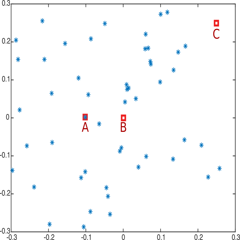
The dataset was generated with the telescope model described in Section 2. 50 stars distributed randomly across the field of view were generated. Their positions are shown on Figure 2. Their fluxes were adjusted such that $26000$ photons on average were recorded per star ; that corresponds to a maximum intensity of $256$ photons in the brightest pixel of the $1500\times 1500$ pixels PSF. To simulate the detector, we add background noise of $5\,e^{-}$ and generate the data $\boldsymbol{d}^{s}$ using the Poisson distribution $\mathcal{P}$:

$$d_{n}^{s}=\mathcal{P}(\left|w^{s}_{K,n}\right|^{2}+5)\,.$$ (18)

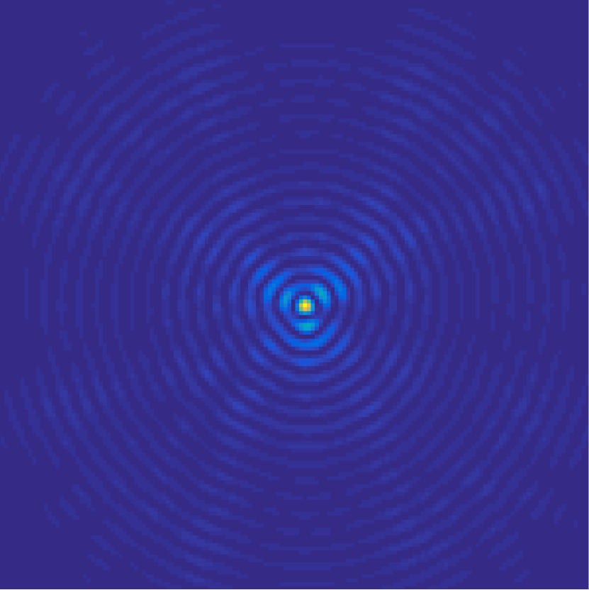
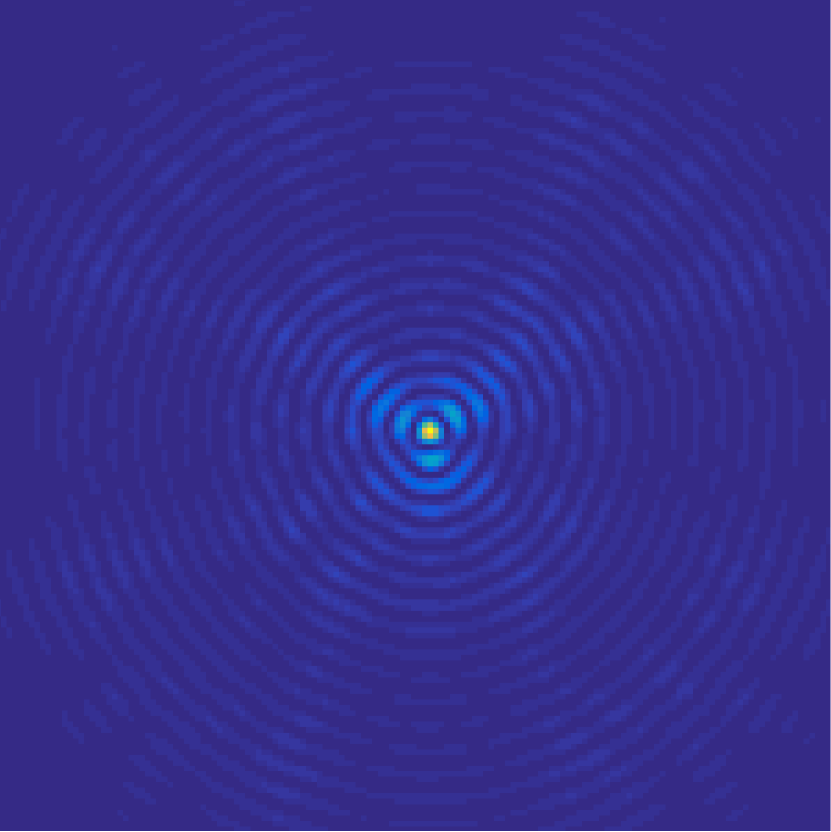
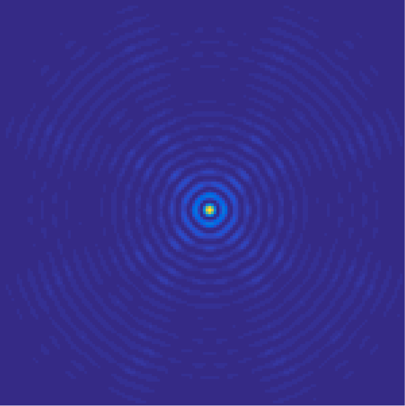
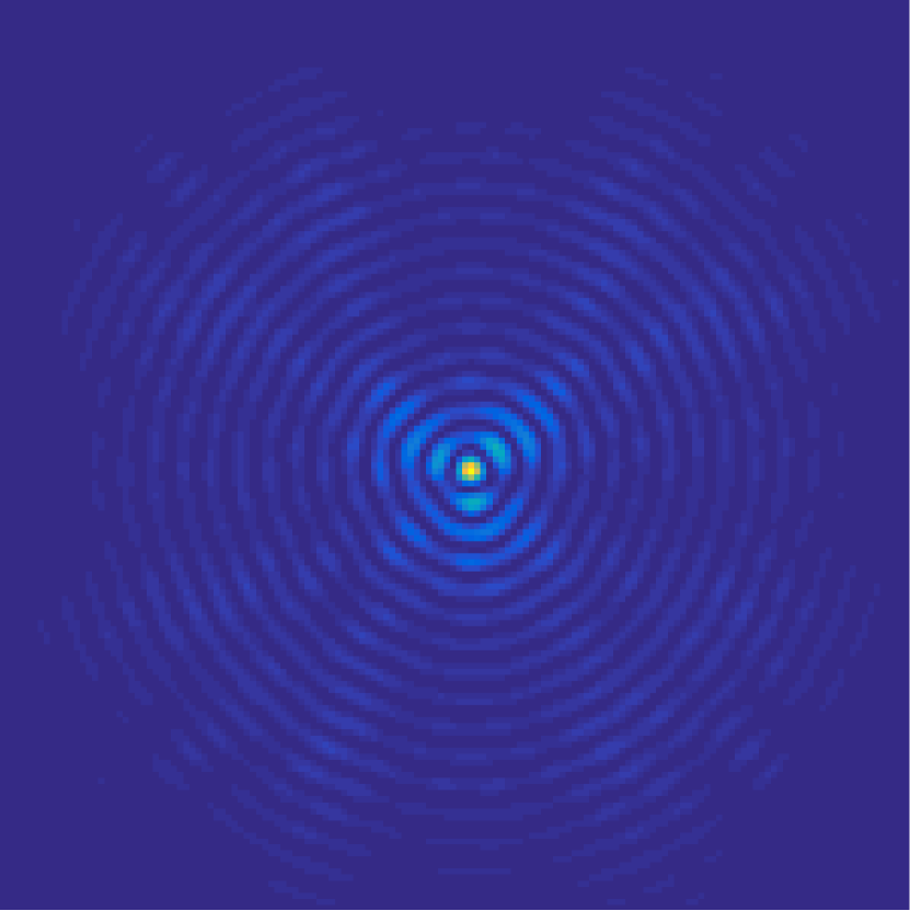
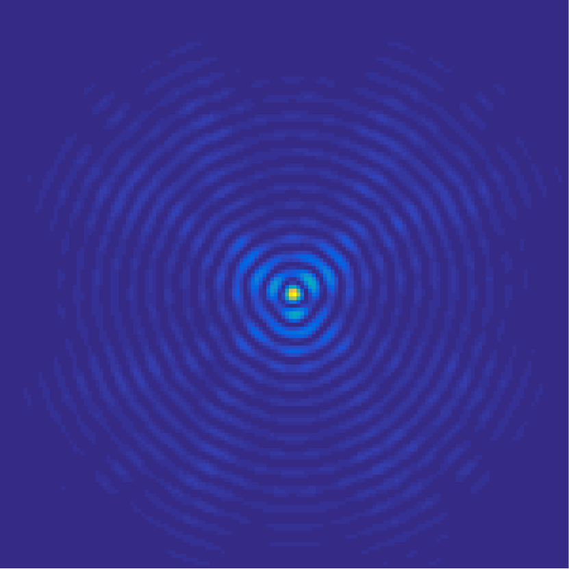
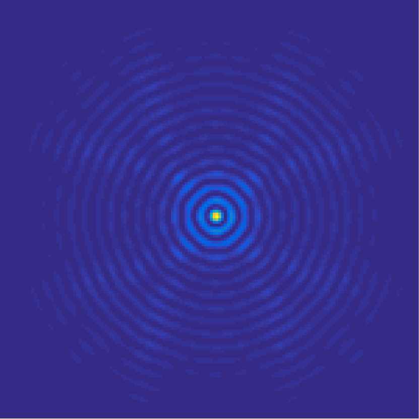
The $300\times 300$ pixels central part of the observation of the star indicated by an A on Figure 2 is shown on Figure 2.

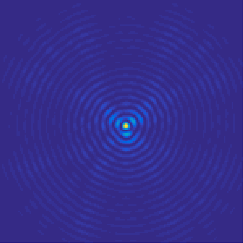
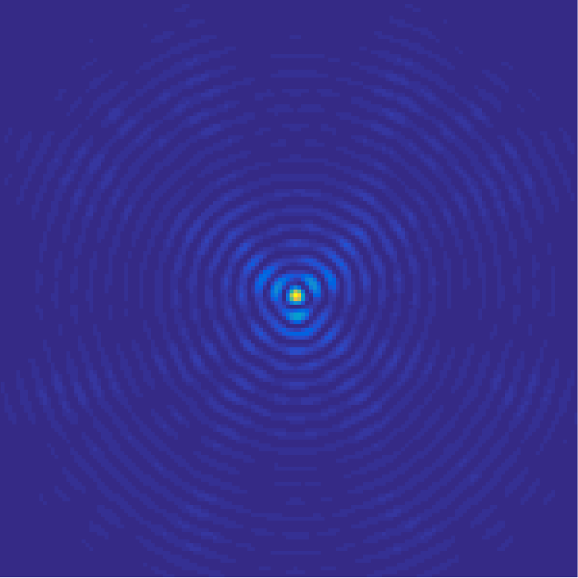
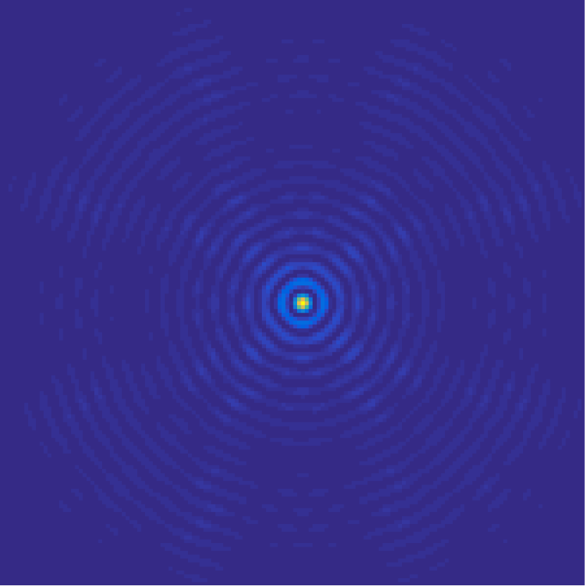
We minimized Equation 12 using the unaberrated telescope as a starting point $\boldsymbol{\alpha}=\boldsymbol{0}$. To assess the performance of our method, we simulate observations of stars that were not in the data-set (denoted as B and C on Figure 2) using our aberrations estimate, the true aberrations and without any aberrations. These stars B and C and one of the star used in aberrations estimation (A) shown on Figure 3. On this figure, we can see that, beginning from an aberration free model, our algorithm successfully converges toward a PSF very similar to the ground truth.

5 Conclusion and future works

In this proof of concept paper, we show the validity of our approach to estimate PSFs at every positions across the field of view without any need to carry out in-flight telescope defocusing to measure directly the wavefront. It achieves to provide qualitatively good PSF even in noisy conditions and we are working on quantitative results in term of ellipticiy and size of the estimated PSF. In addition a lot of works has to be done to be able to process real data, particularly it has to handle undersampled and broadband PSFs.

References

- [1] Laureijs, R. J., Duvet, L., Escudero Sanz, I., Gondoin, P., Lumb, D. H., Oosterbroek, T., and Saavedra Criado, G., “The Euclid Mission,” in [Space Telescopes and Instrumentation 2010: Optical, Infrared, and Millimeter Wave ], Proc. SPIE 7731, 77311H (July 2010).
- [2] Spergel, D., Gehrels, N., Breckinridge, J., Donahue, M., Dressler, A., Gaudi, B., Greene, T., Guyon, O., Hirata, C., Kalirai, J., et al., “Wide-field infrared survey telescope-astrophysics focused telescope assets wfirst-afta final report,” arXiv preprint arXiv:1305.5422 (2013).
- [3] Mboula, F. N., Starck, J.-L., Ronayette, S., Okumura, K., and Amiaux, J., “Super-resolution method using sparse regularization for point-spread function recovery,” Astronomy & Astrophysics 575, A86 (2015).
- [4] Fienup, J. R., Marron, J. C., Schulz, T. J., and Seldin, J. H., “Hubble space telescope characterized by using phase-retrieval algorithms,” Appl. Opt. 32, 1747–1767 (Apr 1993).
- [5] Fienup, J., “Phase retrieval for undersampled broadband images,” J. Opt. Soc. Am. A 16(7), 1831–1837 (1999).
- [6] Roddier, C. and Roddier, F., “Combined approach to the hubble space telescope wave-front distortion analysis,” Appl. Opt. 32, 2992–3008 (Jun 1993).
- [7] Redding, D., Dumont, P., and Yu, J., “Hubble space telescope prescription retrieval,” Applied optics 32(10), 1728–1736 (1993).
- [8] Lyon, R., Dorband, J., and Hollis, J., “Hubble space telescope faint object camera calculated point-spread functions,” Applied optics 36(8), 1752–1765 (1997).
- [9] Krist, J. E. and Burrows, C. J., “Phase-retrieval analysis of pre-and post-repair hubble space telescope images,” Applied optics 34(22), 4951–4964 (1995).
- [10] Kamilov, U. S., Papadopoulos, I. N., Shoreh, M. H., Goy, A., Vonesch, C., Unser, M., and Psaltis, D., “Learning approach to optical tomography,” Optica 2(6), 517–522 (2015).
- [11] Thiébaut, É., “Optimization issues in blind deconvolution algorithms,” in [Astronomical Telescopes and Instrumentation ], 174–183, International Society for Optics and Photonics (2002).
- [12] Schutz, A., Ferrari, A., Mary, D., Soulez, F., Thiébaut, É., and Vannier, M., “Painter: a spatiospectral image reconstruction algorithm for optical interferometry,” J. Opt. Soc. Am. A 31(11), 2334–2345 (2014).
- [13] Mourya, R., Denis, L., Becker, J.-M., and Thiébaut, E., “Augmented lagrangian without alternating directions: Practical algorithms for inverse problems in imaging,” in [Image Processing (ICIP), 2015 IEEE International Conference on ], 1205–1209, IEEE (2015).