Renormalized parameters and perturbation theory in dynamical mean-field theory for the Hubbard model

Abstract

We calculate the renormalized parameters for the quasiparticles and their interactions for the Hubbard model in the paramagnetic phase as deduced from the low energy Fermi liquid fixed point using the results of a numerical renormalization group calculation (NRG) and dynamical mean-field theory (DMFT). Even in the low density limit there is significant renormalization of the local quasiparticle interaction $\tilde{U}$, in agreement with estimates based on the two-particle scattering theory of Kanamori (1963). On the approach to the Mott transition we find a finite ratio for $\tilde{U}/\tilde{D}$, where $2\tilde{D}$ is the renormalized bandwidth, which is independent of whether the transition is approached by increasing the on-site interaction $U$ or on increasing the density to half-filling. The leading $\omega^{2}$ term in the self-energy and the local dynamical spin and charge susceptibilities are calculated within the renormalized perturbation theory (RPT) and compared with the results calculated directly from the NRG-DMFT. We also suggest, more generally from the DMFT, how an approximate expression for the ${\bf q},\omega$ spin susceptibility $\chi({\bf q},\omega)$ can derived from repeated quasiparticle scattering with a local renormalized scattering vertex.

I Introduction

The strong suppression of charge fluctuations and enhancement of magnetic fluctuations in metallic systems with narrow energy bands, derived from atomic-like d or f states, are a reflection of the strong renormalization of the low energy quasiparticles in these systems. The extremely large effective masses, due to the very small quasiparticle weight factor $z$, has led to the classification of many metallic rare earth and actinide metallic compounds as ‘heavy fermion’ systemsStewart (1984); Fisk et al. (1995). In some situations the quasiparticles disappear entirely at a quantum critical point as $z\to 0$ leading to finite temperature non-Fermi liquid behaviorColeman et al. (2001); Löhneysen et al. (2007); Si and Steglich (2010). In the cuprate superconductors the apparent breakdown of Fermi liquid behavior appears to be closely associated with a possible electronic mechanism for pairing leading to high temperature superconductivity in these materialsTaillefer (2010); Plakida .

The basic mechanism driving these strong renormalization effects is believed in most cases to be the strong local Coulomb interactions in the d or f shell orbitals. This renormalization is very well understood in impurity systems where the strong local interaction is solely at the impurity site, as described in the single impurity Anderson model. This understanding is based on very effective non-perturbative techniques, such as the numerical renormalization group (NRG), Bethe Ansatz (BA), conformal field theory (CFT), slave bosons and $1/N$ expansionsWilson (1975); Tsvelik and Wiegmann (1983); Andrei et al. (1983); Affleck and Ludwig (1993); Coleman (1984); Hewson (1997). The leading low energy effects can also be calculated exactly in terms of quasiparticles and their interactions in a renormalized perturbation theoryHewson (1993, 2006) (RPT). The breakdown of the quasiparticles has also been described quantitatively in certain impurity models using these techniquesNishikawa et al. (2012a, b).

The corresponding generic lattice model describing electrons in a narrow conduction bands is the Hubbard modelHubbard (1963). Progress in understanding this model has been much more limited, except for the model in one dimension, where an exact solution has been obtained based on the Bethe AnsatzLieb and Wu (1968, 2003). Models in one dimension, however, are known to be untypical of higher dimensional systems as the low energy excitations are collective bose-like excitations, and correspond to Luttinger liquids rather the Fermi liquidsHaldane (1981). One non-perturbative technique, dynamical mean-field theory (DMFT), has proved to be very effective in leading to an understanding of the metal to insulator, the Mott-Hubbard transition, in the Hubbard and related models. This approach is based on mapping the model into an effective impurity model, which can then be solved using an ’impurity solver’; the most commonly used being the numerical renormalization group methodBulla et al. (2008) (NRG) or the Monte Carlo methodJarrell (1992); Georges and Krauth (1992) (MC). This mapping involves an approximation, but can be shown to be exact in the infinite dimensional limit, and to be a good approximation in systems where the self-energy is strongly frequency dependent and has only a weak wavevector dependence, which is the usual situation in three dimensional strongly correlated metals. The earlier papers using this approach, with a detailed description of the application to the Mott-Hubbard transition were reviewed in the article by Georges et al. Georges et al. (1996). More recent developments have been the application to models for particular metallic compounds, and to include finite dimensional effects which involve a mapping onto to an effective cluster model rather than an impurity modelPark et al. (2008); Fuchs et al. (2011).

Though there have been many studies of the Hubbard and related models using the dynamical mean-field theory, the nature of the low energy quasiparticles and their interactions has received little attention. In an earlier study we considered how the quasiparticles for the Hubbard model vary in the presence of a magnetic fieldBauer and Hewson (2007a) and also in an antiferromagnetic state Bauer and Hewson (2007b). There have been recent studies of the HubbardLogan and Galpin (2016) and the related $t-J$ modelShastry and Perepelitsky (2016) concentrating the region of the Mott-Hubbard transformation. It is of interest, therefore, to examine how the quasiparticles and their interactions are modified in this regime, as the quasiparticle weight $z\to 0$ on the approach to the transition and the quasiparticles disappear. Here we calculate the quasiparticle renormalizations by analyzing the low energy NRG fixed point from a DMFT-NRG calculation. We can, not only characterize the free quasiparticles, but also deduce the renormalized on-site quasiparticle interaction. The fact that the self-energy of the effective impurity is the same as that for the on-site Green’s function of the lattice in the DMFT means it can be calculated using the renormalized perturbation theory for the effective impurity. This is one of the few analytic approaches which is applicable in the strong correlation regime. Some of the results, such as those for the local spin and charge excitations, and the leading $\omega^{2}$ can be checked against those deduced from the NRG calculations. However, expressions for ${\bf q}$ and $\omega$ dependent response functions, based on repeated quasiparticle scattering, go beyond the quantities that can be calculated directly using the DMFT.

In section II of the paper we give background details of the model, and the equations used in the DMFT and RPT. In section III we survey the results for the renormalized parameters in the different regimes, and section V look at the low energy behaviour of the self-energy. In section VI we consider the application of the RPT to the calculation of local spin and charge dynamic susceptibilities, and in VII suggest more generally how the corresponding ${\bf q}$ and $\omega$ dependent susceptibilities be might estimated from repeated quasiparticle scattering with a local renormalized interaction vertex. Finally in section VIII we provide a summary and discuss the possibilities for further developments using this approach.

II Dynamical mean-field approach and renormalized parameters

The Hamiltonian for the single band Hubbard model in a magnetic field is given by

$$H_{\mu}=-\sum_{i,j,\sigma}(t_{ij}c^{\dagger}_{i,\sigma}c_{j,\sigma}+\mathrm{h.c.})-\sum_{i\sigma}\mu_{\sigma}n_{i\sigma}+U\sum_{i}n_{i,\uparrow}n_{i,\downarrow},$$ (1)

where $t_{ij}$ are the hopping matrix elements between sites $i$ and $j$, $U$ is the on-site interaction; $\mu_{\sigma}=\mu+\sigma h$, where $\mu$ is the chemical potential of the interacting system, and the Zeeman splitting term with external magnetic field $H$ is given by $h=g\mu_{\rm B}H/2$, where $\mu_{\rm B}$ is the Bohr magneton.

From Dyson’s equation, the one-electron Green’s function $G_{{\bf k},\sigma}(\omega)$ can be expressed in the form,

$$G_{{\bf k},\sigma}(\omega)=\frac{1}{\omega+\mu_{\sigma}-\Sigma_{\sigma}({\bf k},\omega)-\varepsilon({\bf k})},$$ (2)

where $\Sigma_{\sigma}({\bf k},\omega)$ is the proper self-energy, and $\varepsilon({\bf k})=\sum_{\bf k}e^{-{\bf k}\cdot({\bf R}_{i}-{\bf R}_{j})}t_{ij}$. The simplification that occurs for the model in the infinite dimensional limit is that $\Sigma_{\sigma}({\bf k},\omega)$ becomes a function of $\omega$ only Metzner and Vollhardt (1989); Müller-Hartmann (1989), so the local Green’s function $G_{\sigma}^{\mathrm{loc}}(\omega)$ takes the form,

$$G_{\sigma}^{\mathrm{loc}}(\omega)=\sum_{\bf k}G_{{\bf k},\sigma}(\omega)=\!\int\limits\!\!{\rm d}\varepsilon\;\frac{D(\varepsilon)}{\omega+\mu_{\sigma}-\Sigma_{\sigma}(\omega)-\varepsilon},$$ (3)

where $D(\varepsilon)$ is the density of states for the non-interacting model ($U=0$). In the dynamical mean-field theory approach Georges et al. (1996), an auxiliary Green’s function, ${\cal G}_{0,\sigma}(\omega)$, is introduced such that

$${\cal G}_{0,\sigma}^{-1}(\omega)=G_{\sigma}^{\mathrm{loc}}(\omega)^{-1}+\Sigma_{\sigma}(\omega),$$ (4)

which can be written as

$$G^{\mathrm{loc}}_{\sigma}(\omega)=\frac{1}{{\cal G}_{0,\sigma}^{-1}(\omega)-\Sigma_{\sigma}(\omega)}.$$ (5)

This local Green’s function $G_{\sigma}^{\mathrm{loc}}(\omega)$ can be identified as the Green’s function $G^{\rm imp}_{\sigma}(\omega)$ of an effective single impurity Anderson model, and the auxiliary Green’s function, ${\cal G}_{0,\sigma}(\omega)$, interpreted as the local Green’s function for the non-interacting effective impurity. If we re-express ${\cal G}_{0,\sigma}^{-1}(\omega)$ in the form,

$${\cal G}_{0,\sigma}^{-1}(\omega)=\omega+\mu+\sigma h-K_{\sigma}(\omega),$$ (6)

then Eqn. (5) corresponds to the equation for the impurity Green’s function in a more conventional form,

$$G^{\rm imp}_{\sigma}(\omega)=\frac{1}{\omega-\varepsilon_{\mathrm{d}\sigma}-K_{\sigma}(\omega)-\Sigma_{\sigma}(\omega)},$$ (7)

where $\varepsilon_{\mathrm{d}\sigma}=-\mu_{\sigma}$ plays the role of the impurity level, and $K_{\sigma}(\omega)$ is the hybridization term. In the impurity case in the wide band limit $K_{\sigma}(\omega)$ can be taken as $-i\Delta$ where $\Delta$ is a constant. From Eqns. (3) and (4) it follows that for the lattice model $K_{\sigma}(\omega)$ is a function of the self-energy $\Sigma_{\sigma}(\omega)$. In the presence of an applied magnetic field it will also depend on the value of the field and on $\sigma$. As this self-energy is identified with the impurity self-energy, which in turn depends on the form taken for $K_{\sigma}(\omega)$, then $K_{\sigma}(\omega)$ has to be determined self-consistently and so plays the role of an effective dynamical field. To define the model completely, we need to specify the density of states $D(\omega)$ of the non-interacting model. For the infinite dimensional model this is usually taken to be either that for a tight-binding hypercubic or that for a Bethe lattice. Here we take the semi-elliptical form corresponding to a Bethe lattice,

$$D(\varepsilon,\mu)=\frac{2}{\pi D^{2}}\sqrt{D^{2}-(\varepsilon+\mu)^{2}},$$ (8)

where $2D$ is the band width, with $D=2t$ for the Hubbard model, and $\mu$ the chemical potential of the free electrons. We choose this form with the value $t=1$ throughout, rather than the Gaussian density of states of the hypercubic lattice, as it has a finite bandwidth ($W=4t=4.0$).

The focus here will be on using the renormalized perturbation theory (RPT) in the strongly correlated regime where standard perturbation theory is not applicable.

In formulating RPT approach we assume that the self-energy $\Sigma_{\sigma}(\omega)$ can be written in the form

$$\Sigma_{\sigma}(\omega)=\Sigma_{\sigma}(0)+\omega\Sigma^{\prime}_{\sigma}(0)+\Sigma_{\sigma}^{\rm rem}(\omega),$$ (9)

which corresponds to an expansion in powers of $\omega$ to first order but includes a remainder term $\Sigma_{\sigma}^{\rm rem}(\omega)$. We assume the Luttinger result that the imaginary part of the self-energy behaves asymptotically as $\omega^{2}$ as $\omega\to 0$, so that both $\Sigma_{\sigma}(0)$ and $\Sigma^{\prime}_{\sigma}(0)$ can be taken to be realLuttinger (1960). These two assumptions imply that the low energy fixed point corresponds to a Fermi liquid. No terms have been omitted so, apart from these assumptions, there is no approximation involved. Substituting this form for the self-energy into Eqn. (2), it can be written in the form

$$G_{{\bf k},\sigma}(\omega)=\frac{z_{\sigma}}{\omega+\tilde{\mu}_{\sigma}-\tilde{\Sigma}_{\sigma}(\omega)-\tilde{\varepsilon}_{\sigma}({\bf k})},$$ (10)

where

$$\tilde{\mu}_{\sigma}=z_{\sigma}(\mu_{\sigma}-\Sigma_{\sigma}(0)),\quad z_{\sigma}=1/[1-\Sigma^{\prime}_{\sigma}(0)],$$ (11)

$\tilde{\varepsilon}(\sigma,{\bf k})=z_{\sigma}\varepsilon({\bf k})$ and $\tilde{\Sigma}_{\sigma}(\omega)$ is the renormalized self-energy defined by

$$\tilde{\Sigma}_{\sigma}(\omega)=z_{\sigma}\Sigma^{\rm rem}_{\sigma}(\omega).$$ (12)

We interpret $z_{\sigma}$ as a quasiparticle weight factor, and define a quasiparticle Green’s function, $\tilde{G}_{{\bf k},\sigma}(\omega)$, for the interacting system as

$$\tilde{G}_{{\bf k},\sigma}(\omega)=\frac{1}{\omega+\tilde{\mu}_{\sigma}-\tilde{\Sigma}_{\sigma}(\omega)-\tilde{\varepsilon}_{\sigma}({\bf k})},$$ (13)

which is now similar in form to that given in Eqn. (2). The free quasiparticle Green’s function, $\tilde{G}_{{\bf k},\sigma}(\omega)$, corresponds to putting $\tilde{\Sigma}_{\sigma}(\omega)=0$ in Eqn. (13).

Using the same expression for the self-energy in the local Green’s function (3), it can be rewritten in the form,

$$G_{\sigma}^{\mathrm{loc}}(\omega)=z_{\sigma}\!\int\limits\!\!{\rm d}\varepsilon\;\frac{D(\varepsilon/z_{\sigma})}{\omega+\tilde{\mu}_{\sigma}-\varepsilon-\tilde{\Sigma}_{\sigma}(\omega)}.$$ (14)

The local free quasiparticle propagator, $G_{0,\sigma}^{\mathrm{loc}}(\omega)$, is given by

$$\tilde{G}_{0,\sigma}^{\mathrm{loc}}(\omega)=\!\int\limits\!\!{\rm d}\varepsilon\;\frac{D(\varepsilon/z_{\sigma})}{\omega+\tilde{\mu}_{\sigma}-\varepsilon}.$$ (15)

The density of states $\tilde{\rho}_{\sigma}(\omega)$ derived from this Green’s function via $\tilde{\rho}_{\sigma}(\omega)=-{\rm Im}\tilde{G}_{0,\sigma}(\omega+i\delta)/\pi$ we will refer to as the free quasiparticle density of states (DOS). For the Bethe lattice, this DOS takes the form of a band with renormalized parameters,

$$\tilde{\rho}_{\sigma}(\omega)=\frac{2}{\pi\tilde{D}_{\sigma}^{2}}\sqrt{\tilde{D}_{\sigma}^{2}-(\omega+\tilde{\mu}_{\sigma})^{2}},$$ (16)

where $\tilde{D}_{\sigma}=z_{\sigma}D$.

The renormalized perturbation theory is set up such that the propagators used in the expansion correspond to the fully dressed non-interacting quasiparticles, and the expansion is in powers of the quasiparticle interaction which is identified with full four-vertex between spin up and spin down electrons on the same site $i$ evaluated with all the frequency arguments set to zero,

$$\tilde{U}=z_{\uparrow}z_{\downarrow}\Gamma^{(4)}_{i\uparrow,i\downarrow,i\downarrow,i\uparrow}(0,0,0,0).$$ (17)

This vertex with zero frequency arguments is well defined in the finite frequency $T=0$ perturbation theory, and being a local vertex with the all site indices corresponding to a single site is the same for the effective impurity and lattice in the infinite dimensional limit. Counter terms must be included in the calculation to cancel off any renormalizations which may be generated in the expansion. As the quasiparticles are taken to be fully renormalized any further renormalization would result in overcounting.

We will need the values of the renormalized parameters to substitute in the RPT and these we deduce from the NRG calculation for the effective impurity. We first consider how to calculate the parameters $z_{\sigma}$ and $\tilde{\mu}_{\sigma}$ which characterise the free quasiparticles. For the NRG calculations for the Anderson model the conduction electron density of states is discretized and transformed into a form which corresponds to a one dimensional tight binding chain. This conduction electron chain is then coupled via an effective hybridization $V_{\sigma}$ to the impurity Krishna-murthy et al. (1980). In this representation $K_{\sigma}(\omega)=|V_{\sigma}|^{2}g_{0,\sigma}(\omega)$, where $g_{0,\sigma}(\omega)$ is the one-electron Green’s function for the first site of the isolated conduction electron chain. We substitute the self-energy $\Sigma_{\sigma}(\omega)$ into the form given earlier into Eqns. (9) and (7),

$$G^{\rm imp}_{\sigma}(\omega)=\frac{z_{\sigma}}{\omega-\tilde{\varepsilon}_{\mathrm{d}\sigma}-|\tilde{V}_{\sigma}|^{2}g_{0,\sigma}(\omega)-\tilde{\Sigma}_{\sigma}(\omega)},$$ (18)

where

$$\tilde{\varepsilon}_{\mathrm{d}\sigma}=z_{\sigma}(\varepsilon_{\mathrm{d}\sigma}+\Sigma_{\sigma}(0)),\quad|\tilde{V}_{\sigma}|^{2}={z_{\sigma}}|V_{\sigma}|^{2}.$$ (19)

The corresponding free quasiparticle impurity Green’s function, $\tilde{G}^{\rm imp}_{0,\sigma}(\omega)$, is then given by

$$\tilde{G}^{\rm imp}_{0,\sigma}(\omega)=\frac{1}{\omega-\tilde{\varepsilon}_{\mathrm{d}\sigma}-|\tilde{V}_{\sigma}|^{2}g_{0,\sigma}(\omega)}.$$ (20)

As we identify $G^{\rm imp}_{\sigma}(\omega)$ with the local Green’s function for the lattice (3), it follows that

$$\tilde{G}_{0,\sigma}^{\mathrm{loc}}(\omega)=\tilde{G}^{\rm imp}_{0,\sigma}(\omega),$$ (21)

which specifies the form of $g_{0,\sigma}(\omega)$ in (20) and yields $\tilde{\mu}_{\sigma}=-\tilde{\varepsilon}_{\mathrm{d}\sigma}$. By fitting the lowest lying poles of this Green’s function to the lowest lying single particle and hole excitations in the NRG results, we can deduce the parameters $\tilde{\varepsilon}_{\mathrm{d}\sigma}$ and $\tilde{V}_{\sigma}$, as has been explained in earlier work. Hewson et al. (2004). The quasiparticle weight $z_{\sigma}$ is then obtained from the relation $z_{\sigma}=|\tilde{V}_{\sigma}/V_{\sigma}|^{2}$ in Eqn. (19), and $\tilde{\mu}_{\sigma}$ from $\tilde{\mu}_{\sigma}=-\tilde{\varepsilon}_{\mathrm{d}\sigma}$.

We also need to calculate the renormalized on-site interaction $\tilde{U}$ for the effective impurity. This can be deduced from the difference in energies between the lowest lying two-particle excitation from the NRG ground state and the corresponding two free single particle excitations. This procedure is difficult to summarize, so we refer to the earlier work for details in Ref. Hewson et al., 2004.

III Results for Renormalized Parameters

Here we use the NRG method to solve the DMFT equations for the effective impurity to calculate the renormalized parameters $z=\tilde{D}/D$, $\tilde{\mu}_{\sigma}$ and $\tilde{U}$ in different parameter regimes. In the half-filled case in the absence of a magnetic field $\tilde{\mu}_{\sigma}=0$, so we have just two parameters to determine, $z=\tilde{D}/D$ and $\tilde{U}$. These are plotted as a function of $U$ in Fig. 1. For small $U$, $\tilde{U}$ is, as expected, proportional to $U$ up to a value of $U\sim 1$. As the Mott transition is approached at a critical value $U_{c}=5.98$Bulla (1999) (as $D=2$ in our case $U_{c}/D=2.99$), it can be seen that both $\tilde{U}$ and $z$ approach zero in a similar way. If we form the dimensionless ratio $\tilde{U}\tilde{\rho}(0)$, then with $\tilde{\mu}=0$, $\tilde{\rho}(0)=2/\pi\tilde{D}$, we find that $\tilde{U}\tilde{\rho}(0)\to 0.815$ as $U\to U_{c}$. We also see from Eqn. (16) that as $\tilde{D}\to 0$, that the quasiparticle density of states narrows to a delta function at $\omega=0$ as $U\to U_{c}$.

We can define a quasiparticle occupation number $\tilde{n}_{\sigma}$ at $T=0$, by integrating the free quasiparticle density of states up to the Fermi level

$$\tilde{n}_{\sigma}=\int_{-\infty}^{0}d\omega\tilde{\rho}_{\sigma}(\omega).$$ (22)

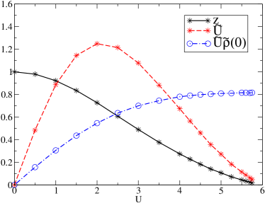
Figure 1: The quasiparticle weight $z=\tilde{D}/D$, the on-site quasiparticle interaction $\tilde{U}$, and the product $\tilde{U}\tilde{\rho}(0)$ for the model at half-filling as a function of $U$

We can also calculate the expectation value of the occupation number $n_{\sigma}$ of the interacting system at $T=0$ using a generalization of Luttinger’s theorem Luttinger and Ward (1960) for each spin component,

$$n_{\sigma}=\!\int\limits_{-\infty}^{\infty}\!\!{\rm d}\varepsilon\;D(\varepsilon)\theta(\mu_{\sigma}-\Sigma_{\sigma}(0)-\varepsilon),$$ (23)

where $\theta(\varepsilon)$ is the Heaviside step function and $D(\varepsilon)$ as given in Eqn. (8). It can be shown that this result is equivalent to that given in Eqn. (22) so $\tilde{n}_{\sigma}=n_{\sigma}$, and hence we can calculate the occupation number $n_{\sigma}$ from the quasiparticle density of states $\tilde{\rho}_{\sigma}(\omega)$.

We can evaluate the integral in Eqn. (22) explicitly in the case of a semi-elliptical density of states, which gives

$$\tilde{n}_{\sigma}=n_{\sigma}={1\over\pi}\left[{\pi\over 2}+{\rm sin}^{-1}\left({\tilde{\mu}_{\sigma}\over\tilde{D}}\right)+{\tilde{\mu}_{\sigma}\over\tilde{D}^{2}}\sqrt{\tilde{D}^{2}-\tilde{\mu}_{\sigma}^{2}}\right].$$ (24)

The magnetization $m(h)$ can be deduced from (24) using $m(h)=g\mu_{\rm B}(n_{\uparrow}-n_{\downarrow})$. In the half-filled case and in the absence of a magnetic field, $\tilde{\mu}=0$, and we see that $\tilde{n}_{\sigma}=0.5$, so it is even possible to assign a value in the localized limit when $z\to 0$, and the quasiparticle density of states collapses to a delta-function.

In Fig. 2 we give a plot of the renormalized chemical potential $\tilde{\mu}$ as a function of $\bar{\mu}=\mu-0.5U$ ($\bar{\mu}=0$ corresponds to the particle-hole symmetry) for $U=3,4,5,6$. For these values up to $U=5$ we are in the metallic regime, so $\tilde{\mu}$ is a continuous function of $\bar{\mu}$, but as $U$ increases there a plateau region develops about $\bar{\mu}=0$, corresponding to a strong correlation regime and a reduced charge susceptibility. For $U=6$ we are very slightly above the critical value $U=5.98$ but so close that the discontinuity is not evident.

We can check the relation in Eqn. (24) for the occupation number $n$ by comparing the values deduced by substituting the results for $\tilde{\mu}$ and $\tilde{D}$ into (24) with those deduced from a direct evaluation of the expectation value of $n$ in the ground state. The results are plotted Fig. 3 as a function of $\bar{\mu}$ for $U=3,4,5,6$. The occupation number $n$ for the non-interacting case $U=0$ is shown for comparison. The values calculated from Eqn. (24) (crosses) and by direct NRG calculation (circles) can be seen to be in excellent agreement (within about 1%). If we assume the relation, $\tilde{n}_{\sigma}=n_{\sigma}$, then the agreement can alternatively be regarded as a check on the calculation of the renormalized parameters, $\tilde{\mu}$ and $\tilde{D}$. The effects of strong correlation leading to a plateau region at the point of half-filling are also evident in this plot.

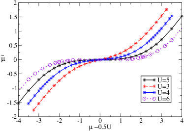
Figure 2: The quasiparticle chemical potential $\tilde{\mu}$ as a function of the on-site occupation $n$ plotted as a function of $\bar{\mu}=\mu-U/2$ for $U=3,4,5,6$.

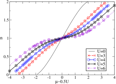
Figure 3: The occupation number $n$ as a function of $\bar{\mu}=\mu-0.5U$ for $U=0,3,4,5,6$, as calculated directly from the DMFT (circles) and from the NRG fixed point(crosses). The flattening of the curve in the region $n\sim 1$ for the larger value of $U$ indicates the strong correlation regime.

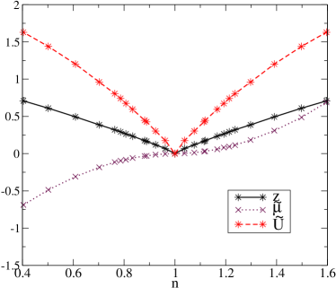
Figure 4: The quasiparticle weight $z=\tilde{D}/D$, the renormalized chemical potential $\tilde{\mu}$ and the on-site quasiparticle interaction $\tilde{U}$ for the model as a function of the occupation number $n$ for $U=6.0$.

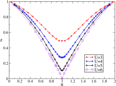
Figure 5: The quasiparticle weight factor $z$ as a function of the occupation number $n$ for $U=3,4,5,6$.

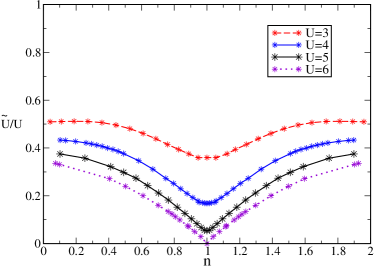
Figure 6: The ratio of $\tilde{U}/U$ as a function of the occupation number $n$ for $U=3,4,5,6$. It can be seen that there is still some significant renormalization of this quantity in the low particle density ($n\to 0$) and low hole density regimes ($n\to 2$).

In Fig. 4 we give show the results for $\tilde{U}$, $z=\tilde{D}/D$ and $\tilde{\mu}$ as a function of the filling factor $n=\sum_{\sigma}n_{\sigma}$ for a value of $U=6$. As this value of $U$ is greater than $U_{c}$, the critical value for the Mott transition at half-filling, $z\to 0$ as the limit of half-filling $n\to 1$ is approached. We also find the $\tilde{U}\tilde{\rho}_{\sigma}$ tends to the same value $\sim 0.815$ as $n\to 1$, so that the values are independent of whether we approach the critical point for the Mott transition by increasing $U$ at half-filling or with $U>U_{c}$ and letting $n\to 1$. The renormalized quasiparticle chemical potential $\tilde{\mu}$ is negative and approaches zero as $n\to 1$.

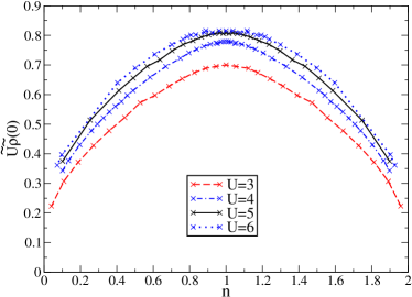
Figure 7: $\tilde{U}\tilde{\rho}(0)$ as a function of $n$ for $U=3,4,5,6$.

In Fig. 5 and Fig. 6 we plot the quasiparticle weight factor $z$ and the ratio $\tilde{U}/U$ as a function of the filling factor $n$. There is marked minimum in both curves at the half-filling point, which is more pronounced for the larger value of $U$. If these are compared with those for the Anderson impurity modelHewson et al. (2006) it can be seen that there is a significant difference in the behaviour of $\tilde{U}/U$ in the regimes $n\to 0$ and $n\to 2$. In the impurity case $\tilde{U}/U\to 1$ so that the renormalization effects are negligible in these limits, whereas for the Hubbard model there is still some significant renormalization due to the phase space available for scattering. This can be estimated following Kanamori Kanamori (1963), who calculated an effective interaction $U_{\rm eff}$, using perturbation theory for the lattice model, taking into account the renormalization due to repeated particle-particle scattering, which is the dominant process in the low density limit. This calculation takes the form,

$$U_{\rm eff}={U\over 1-U\Pi^{p,\uparrow}_{p,\downarrow}(0)},$$ (25)

where the particle-particle propagator $\Pi^{p,\uparrow}_{p,\downarrow}(0)$ at zero frequency in the low density limit is given by

$$\Pi^{p,\uparrow}_{p,\downarrow}(0)=\int_{-D}^{D}\int_{-D}^{D}{D(\varepsilon,-D)D(\varepsilon^{\prime},-D)\over(\varepsilon+\varepsilon^{\prime})}d\varepsilon d\varepsilon^{\prime}.$$ (26)

The evaluation of (26) using the density of states given in Eqn. (8) for $D=2$, gives $\Pi^{p,\uparrow}_{p,\downarrow}(0)=-0.3023$. The results for $U_{\rm eff}$ are then $U_{\rm eff}/U=0.524,\,0.453,\,0.398,\,0.355$, for $U=3,4,5,6$. We can identify $U_{\rm eff}$ as $\tilde{U}$ in the low density regime. From the results given in Fig. 6 we estimate these as $\tilde{U}/U=0.51,\,0.44,\,0.37,\,0.34$ for $U=3,4,5,6$ respectively. These are clearly in general agreement with the Kanamori estimate, slightly smaller but by less than 5% difference in all cases. The quasiparticle weight factor $z$ in the lattice case does approach unity as $n\to 0$ and $n\to 2$ as in the impurity case.

In Fig. 7 we plot the dimensionless product $\tilde{U}\tilde{\rho}(0)$ which gives a measure of relative the strength of the on-site quasiparticle interaction. For the single impurity Anderson model in the Kondo limit $\tilde{U}\tilde{\rho}(0)\to 1$. For the Hubbard model it can be seen to increase steadily on the approach to the most strongly correlated situation at half-filling. As noted earlier in the approach to the Mott transition, either by increasing $U\to U_{c}$ at half-filling or as $n_{d}\to 1$ for $U>U_{c}$, we get the same limiting value $\tilde{U}\tilde{\rho}(0)\to 0.815$. Almost the same limiting value has been obtain for this quantity in studies of the Hubbard-Holstein model both on the approach to the Mott transition and also in the localized limit due to bipolaron formationBauer and Hewson (2010). In the impurity case the result $\tilde{U}\tilde{\rho}(0)\to 1$ could be deduced from the condition that the charge susceptibility tends to zero in the strong correlation regime. For the Hubbard model we do not have an exact result for the charge susceptibility in terms of renormalized parameters to see if a similar argument could be used to deduce the limiting value of $\tilde{U}\tilde{\rho}(0)$ on the approach to the Mott transition.

IV Static Response Functions

If we express the zero temperature static response function $\chi$ in the form,

$$\chi=\tilde{\eta}\tilde{\chi}^{0},$$ (27)

where $\tilde{\chi}^{0}$ is the corresponding function evaluated for the renormalized but non-interacting quasiparticles, then the coefficient $\tilde{\eta}$, is a dimensionless quantity and a measure of the effect of the quasiparticle interactions. In the non-interacting case $U=0$, $\tilde{\eta}=1$ as $\tilde{\chi}^{0}=\chi$. On the approach to a quantum critical point, if the non-interacting quasiparticle susceptibility $\tilde{\chi}^{0}$ diverges, the corresponding susceptibility $\chi$ will also diverge if $\tilde{\eta}$ tends to a finite limit as $z\to 0$. However, not all susceptibilities will be expected to diverge at the transition point, so if $\chi$ remains finite or zero as $z\to 0$ and $\tilde{\chi}^{0}$ diverges, then we require $\tilde{\eta}\to 0$.

We can deduce an expression for the zero temperature uniform charge susceptibility $\chi_{c}$ by differentiating Eqn. (24). The susceptibility for the non-interacting quasiparticles in this case given by $\tilde{\chi}^{0}=2\tilde{\rho}(0)$, and $\tilde{\eta}_{c}$ by

$$\tilde{\eta}_{c}=z{d(\tilde{\mu}/z)\over d\mu}.$$ (28)

The coefficient $\tilde{\eta}_{c}$ deduced from Eqn. (28) using the renormalized parameters is plotted in Fig. 8 (crosses) as a function of the site occupation value $n$ for $U=3,4,5,6$. The values of $\tilde{\eta}_{c}$ can alternatively be deduced from $\chi_{c}$ by taking the derivative of the occupation number $n$, as calculated from the NRG ground state, with respect to $\mu$, and dividing the result by $2\tilde{\rho}(0)$. The results of this calculation are shown as circles in Fig. 8. We note that in the low density limit of electrons $n\to 0$, and the corresponding limit for holes $n\to 2$, that the values of $\tilde{\eta}_{c}$ would appear to be lower than that for the ‘bare’ electrons or holes $\tilde{\eta}_{c}=1$, even though $z\to 1$ in these limits. This must be due to fact that there is phase space available for the particle-particle scattering that led to a renormalization of $\tilde{U}$ from the bare value in these limits.

There is a steady decrease in $\tilde{\eta}_{c}$ from the values at $n\sim 0$ and $n\sim 2$ to a minimum at half-filling. The value $\tilde{\eta}_{c}$ at the half-filling is already very small for $U=5$ and goes zero at the transition $U=5.98$. As $\tilde{\rho}(0)$ diverges on the approach to the transition point this implies that the charge susceptibility is either finite or zero in this limit. The fact that the occupation number $n$ versus $\bar{\mu}$ as shown in Fig. 3 becomes flat for $U<U_{c}$, and there is a discontinuous jump in the values of $\bar{\mu}$ between $n\to 1-$ and $n\to 1+$, means that $\chi_{c}\to 0$ as $U\to U_{c}$.

From the NRG results we can calculate the local on-site dynamic charge susceptibility $\chi_{c}^{\rm loc}(\omega)$ at $\omega=0$, which we will denote by $\chi_{c}^{\rm loc}$. We can define a coefficient $\eta_{c}^{\rm loc}$ via the relation, $\chi^{\rm loc}_{c}=2\tilde{\eta}^{\rm loc}_{c}\tilde{\rho}(0)$. The values of $\tilde{\eta}^{\rm loc}_{c}$ deduced from the NRG results are shown as a function of the occupation number $n$ in Fig. 9. The results and general trend are very similar to those for that uniform charge susceptibility shown in Fig. 8.

We find distinct differences, however, between the local and uniform susceptibilities in the case of the spin. The zero field uniform susceptibility at $T=0$ can be expressed in the form,

$$\chi_{s}={1\over 2}(g\mu_{\rm B})^{2}\tilde{\eta}_{s}\tilde{\rho}(0),\quad{\rm where}\quad\tilde{\eta}_{s}={\rm lim}_{h\to 0}{{(\tilde{\mu}_{\uparrow}-\tilde{\mu}_{\downarrow})}\over 2h},$$ (29)

where the factor $\tilde{\eta}_{s}$ is due to the interaction between the quasiparticles, and is equivalent to the usual definition of the Wilson $\chi/\gamma$ ratio. It can be calculated from Eqn. (29) using the results for the renormalized parameters in a magnetic field. Alternatively it can be deduced from the magnetization $m(h)$ calculated from the NRG ground state using $\tilde{\eta}_{s}=\lim_{h\to 0}m(h)/h\tilde{\rho}(0)$. The results for $\tilde{\eta}_{s}$ are shown in Fig. 10 as a function of $n$ for $U=3,4,5$ and $6$. The points marked with a cross indicate those calculated from the renormalized parameters, and those with circles are deduced from the NRG magnetization. The two sets of results are in good agreement. There is a marked change in the form of $\tilde{\eta}_{s}$ on the approach to half-filling as the value of $U$ is increased from 3 to 5. For $U<4$ $\tilde{\eta}_{s}>1$, there is an enhancement of the quasiparticle susceptibility due to the quasiparticle interactions, increasing from the low density regime with a slight peak at half-filling. There is also an enhancement for $U=4$ in the low density regime but a significant dip on the approach to half-filling where it has a minimum with $\tilde{\eta}_{s}\sim 1$. The same trend can be seen for the case $U=5$ but the dip at half-filling is much much greater and such that $\tilde{\eta}_{s}<1$. This means that the quasiparticle interactions are tending to suppress rather than enhance the free quasiparticle susceptibility, which was also found in the calculation of BauerBauer (2009). Such a suppression would be expected from an antiferromagnetic interaction between the quasiparticles. For large $U$ in the localized limit at half-filling the Hubbard model can be mapped into an antiferromagnetic Heisenberg model and has an antiferromagnetic ground state, so the quasiparticle interactions could be precursors of this limit. It would be interesting to calculate $\tilde{\eta}_{s}$ near half-filling for values of $U$ on the approach to the Mott transition $U\to U_{c}$. Unfortunately it becomes very difficult in this regime to achieve self-consistency of the the DMFT equations in very weak magnetic fields in this regime, such that numerically we can make no reliable predictions for the behavior of $\eta_{s}$ as $U\to U_{c}$. However, there is an interesting analogy with a two quantum dot model with an antiferromagnetic interaction between the dots, which has a quantum critical point. In that case, though the quasiparticle weight $z\to 0$ on the approach to the critical point the uniform susceptibility remains finiteNishikawa et al. (2012a, b). This implies $\tilde{\eta}\to 0$ as $z\to 0$. We speculate the something similar might hold in this case also, and the trend seen in Fig. 10 with increasing $U$ will be such that the value of $\tilde{\eta}_{s}$ will dip to zero at half-filling as $U\to U_{c}$. Further evidence to test whether this might be the case could be derived from a calculation of the zero field susceptibility to higher order $\tilde{U}$ in the RPT, along the lines used in Ref. Pandis and Hewson, 2015, and this is under active consideration. The results could also be tested against those deduced from the NRG for a range of values of $U$.

The local spin susceptibility has a completely different behavior on the approach to half-filling. We define $\chi_{s}^{\rm loc}$ as the $\omega=0$ value of the on-site spin correlation function $\chi_{s}^{\rm loc}(\omega)$ which can be calculated using the NRG. We can define an $\eta_{s}^{\rm loc}$ via the relation, $\chi_{s}^{\rm loc}={1\over 2}(g\mu_{\rm B})^{2}\tilde{\eta}_{s}^{\rm loc}\tilde{\rho}(0)$, Results for $\eta_{s}^{\rm loc}$ are shown for $U=3,4,5,6$ in Fig. 11. They all show a steady increase on the approach to half-filling to a finite maximum value at $n=1$. There is only a significant difference between the results for the different values of $U$ in the region near half-filling, the values for larger $U$ being larger.

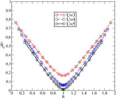
Figure 8: $\tilde{\eta}_{c}=\chi_{c}/\tilde{\chi}_{c}^{(0)}$, where $\chi_{c}$ is the uniform charge susceptibility, plotted as a function of $n$ for $U=3,4,5$.

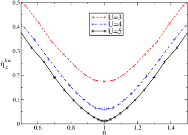
Figure 9: $\tilde{\eta}^{\rm loc}_{c}=\chi^{\rm loc}_{c}/2\tilde{\rho}(0)$, where $\chi^{\rm loc}_{c}$ is the local charge susceptibility, plotted as a function of $n$ for $U=3,4,5$.

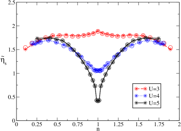
Figure 10: $\tilde{\eta}_{s}=\chi_{s}/\tilde{\chi}_{s}$, where $\chi_{s}$ is the uniform spin susceptibility, plotted as a function of $n$ for $U=3,4,5$.

Figure 11: $\tilde{\eta}^{\rm loc}_{s}=2\chi^{\rm loc}_{s}/\tilde{\rho}(0)$, where $\chi^{\rm loc}_{s}$ is the local spin susceptibility, plotted as a function of $n$ for $U=3,4,5,6$.

V Renormalized Self-Energy Calculations

Having deduced from the NRG the renormalized parameters $\tilde{\mu}$ and $\tilde{D}$, which define the free quasiparticle density of states $\tilde{\rho}_{\sigma}(\omega)$, and the renormalized on-site quasiparticle interaction $\tilde{U}$, from the NRG, we are now in a position to use them in the RPT to calculate the renormalized self-energy $\tilde{\Sigma}_{\sigma}(\omega)$. The perturbation theory can proceed exactly along the same lines as the RPT for the standard single impurity Anderson model. The free quasiparticle Green’s function is $\tilde{G}^{\rm imp}_{0,\sigma}(\omega)$ is the propagator in the expansion which is formally in powers of $\tilde{U}$. The main difference from the usual perturbation theory in powers of the bare parameter $U$ is that the parameter $\tilde{U}$ is already renormalized. As a consequence counter terms have to be included to ensure that there is no overcounting of renormalization effects. These are determined from the conditions that $\tilde{\Sigma}_{\sigma}(0)=0$, $\tilde{\Sigma}^{\prime}_{\sigma}(0)=0$, and that $\tilde{U}=\tilde{\Gamma}^{(4)}_{\uparrow,\downarrow}(0,0,0,0)=z^{2}\Gamma^{(4)}_{\uparrow,\downarrow}(0,0,0,0)$, where $\Gamma^{(4)}_{\uparrow,\downarrow}(\omega_{1},\omega_{2},\omega_{3},\omega_{4})$ is the full local four-vertex.

To test the RPT results for $\tilde{\Sigma}_{\sigma}(\omega)$ in the low energy regime against the NRG calculations for the self-energy $\Sigma_{\sigma}(\omega)$, it will be convenient to use the relation between their imaginary parts,

$${\rm Im}\,\Sigma(\omega)={1\over z}{\rm Im}\,\tilde{\Sigma}(\omega),$$ (30)

which follows directly from the definition of the renormalized self-energy $\tilde{\Sigma}_{\sigma}(\omega)$.

The lowest order correction term for ${\rm Im}\tilde{\Sigma}(\omega)$ is second order in $\tilde{U}$. It has been shown for the particle-hole symmetric Anderson model that this term gives the asymptotically exact result to leading order as $\omega\to 0$ and $T\to 0$, for all values of $U$. This result then enables one to calculate exactly the leading order temperature dependence of the conductivity as $T\to 0$. Here we perform the same calculation using the parameters derived for the lattice and test the results with those derived directly from the NRG. Working to second order in $\tilde{U}$ we can use the standard perturbation theory to evaluate ${\rm Im}\tilde{\Sigma}(\omega)$. The two counter terms that ensure $\tilde{\Sigma}_{\sigma}(0)=0$ and $\tilde{\Sigma}^{\prime}_{\sigma}(0)=0$, to this order are real and do not contribute to the imaginary part of $\tilde{\Sigma}(\omega)$. There is also no counter term correction to the condition $\tilde{U}=\tilde{\Gamma}_{\uparrow,\downarrow}(0,0,0,0)$ to second order. We then find

$${\rm Im}\tilde{\Sigma}(\omega)=\pi\tilde{U}^{2}\int\tilde{\rho}(\varepsilon)\tilde{\rho}(\varepsilon^{\prime})\tilde{\rho}_{(}\omega-\varepsilon-\varepsilon^{\prime})F(\omega,\varepsilon,\varepsilon^{\prime})d\varepsilon d\varepsilon^{\prime},$$ (31)

where

$$F(\omega,\varepsilon,\varepsilon^{\prime})=(1-f(\varepsilon)-f(\varepsilon^{\prime}))f(\varepsilon+\varepsilon^{\prime}-\omega)+f(\varepsilon)f(\varepsilon^{\prime}).$$ (32)

with $f(\varepsilon)=1/(1+e^{\varepsilon/T})$. This leads to the asymptotic form for small $\omega$ and $T$,

$${\rm Im}\,\Sigma(\omega)\sim-{\pi\over 2z}\tilde{\rho}(0)^{3}\tilde{U}^{2}(\omega^{2}+(\pi T)^{2}).$$ (33)

If we introduce a renormalized energy scale via $1/\tilde{\rho}(0)=4T^{*}$ (in an impurity model in the Kondo regime $T^{*}$ corresponds to the Kondo temperature $T_{\rm K}$), then we can rewrite this expression in the form,

$${\rm Im}\Sigma(\omega)=-{\pi C^{2}\over 32\rho(0)}\left[\left({\omega\over T^{*}}\right)^{2}+\left({\pi T\over T^{*}}\right)^{2}\right]+....,$$ (34)

where $C=\tilde{\rho}(0)\tilde{U}$ is a dimensionless parameter. As mentioned earlier $C$ tends to the value $0.816$ in the approach to the Mott transition ($z\to 0$). As a consequence all the renormalized parameters can be expressed in terms of the single energy scale $T^{*}$ on the approach to the Mott transition. This same behavior was already found in a local model, which has two types of zero temperature transitions, on the approach to each critical pointNishikawa et al. (2012a, b). As $4T^{*}=1/\tilde{\rho}(0)$, and at particle-hole symmetry $\tilde{\rho}(0)=2/\pi\tilde{D}$, then $T^{*}=z\pi D/8$, proportional to $z$ so this is also equivalent to the $\omega/z$ scaling found in Ref. Zitko et al., 2013.

We can check the predictions of the RPT for ${\rm Im}\Sigma(\omega)$ by making a comparision with the results for this quantity obtained directly from the NRG calculations. In Fig. 12 we compare with the RPT and NRG results for ${\rm Im}\Sigma(\omega)$ at $T=0$ for the half-filled model with $U=3$. The second order result clearly describes the behaviour over the low energy scale $|\omega|<T^{*}$. Over this region there is very little difference between the full second order result and the asymptotic result (33). In Fig. 13 a similar comparison is made between the NRG and asymptotic result for a larger value $U=5.0$. Again there is good agreement over the range $|\omega|<T^{*}$. It is difficult to make a comparison for larger values of $U$ near the Mott transition as $T^{*}$ becomes very small as $T^{*}\to 0$ for $U\to U_{c}$. Due to the discrete spectrum used for the bath in the NRG calculations, the spectra generated consist of sets of delta functions which have to be broadened to give a continuous spectrum. This broadening factor then introduces errors in determining the coefficient of the $\omega^{2}$ term, which make it difficult to estimate reliably when $T^{*}$ becomes very small.

In Fig. 14 we make a comparison of the results in a case away from half-filling with $U=6.0$ and $x=0.7$. The agreement is again good over the scale $|\omega|<T^{*}$, but the NRG results deviates quite markedly from the RPT second order result for $T^{*}<\omega<2T^{*}$, though it is still a good approximation for $-2T^{*}<\omega<-T^{*}$.

The indication from these results is that the second order RPT result does lead to the correct asymptotic behaviour for the imaginary part of the self-energy, and so these results can be used to calculate the $T^{2}$ coefficient of the conductivity for this model.

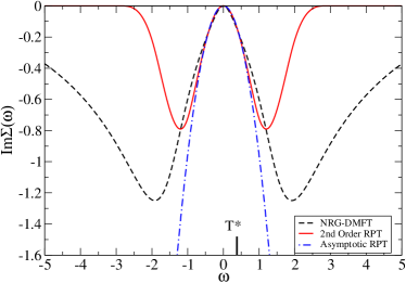
Figure 12: The imaginary part of the self-energy for U=3.0, $T^{*}=0.38$, compared with the corresponding NRG results.

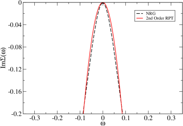
Figure 13: The imaginary part of the self-energy for U=5.0, $T^{*}=0.084$, compared with corresponding NRG results.

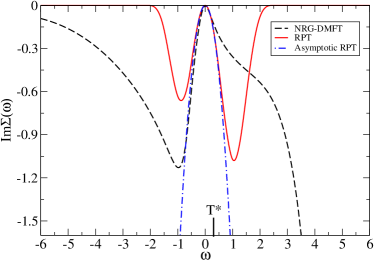
Figure 14: A comparison of the RPT result for the imaginary part of the self-energy for n=0.7, U=6, $T^{*}\sim 0.31$ with the corresponding NRG-DMFT results. There is good agreement for positive $\omega$ up to $\omega\sim T^{*}$ but the agreement extends to larger values of $|\omega|$ on the negative side.

VI Local Dynamic Response Functions

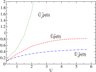
Figure 15: A plot of $\tilde{U}\tilde{\rho}(0)$, $\tilde{U}_{s}\tilde{\rho}(0)$ and $\tilde{U}_{c}\tilde{\rho}(0)$ as a function of $U$ at half-filling.

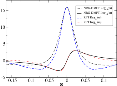
Figure 16: A comparison of NRG-DMFT results for $\chi_{s,l}(\omega)$ with the RPT formula for U=5.6.

The calculations here proceed along similar lines for the effective impurity. The equation for the transverse spin susceptibility is

$$\chi_{s,t}(\omega)={\tilde{\Pi}^{0}(\omega)\over 1-\tilde{U}_{s}^{\rm loc}\tilde{\Pi}^{0}(\omega)},$$ (35)

$\tilde{U}_{s}^{\rm loc}$ is the irreducible quasiparticle interaction in this channel and $\tilde{\Pi}^{0}(\omega)$ is given by

$$\tilde{\Pi}^{0}(\omega)=\int\int{f(\varepsilon)-f(\varepsilon^{\prime})\over(\omega-\varepsilon+\varepsilon^{\prime})}\tilde{\rho}(\varepsilon)\tilde{\rho}(\varepsilon^{\prime})\,d\varepsilon\,d\varepsilon^{\prime},$$ (36)

where $\tilde{\rho}(\omega)$ is the free quasiparticles density of states given in Eqn. (16). In the absence of a magnetic field $\chi_{s,l}(\omega)$ is the same as the transverse response function apart from a factor 2, $\chi_{s,l}(\omega)=0.5\chi_{s,t}(\omega)$. The interaction term $\tilde{U}_{s}^{\rm loc}$ in the scattering channel is not the same as the on-site quasiparticle interaction $\tilde{U}$, calculated earlier, as the $\tilde{U}$, already includes some of these scattering terms for $\omega=0$, so $\tilde{U}_{s}^{\rm loc}=\tilde{U}-\lambda_{3}$, where $\lambda_{3}$ is the counter term associated with the interaction. In the impurity case, assuming a flat wide band for the conduction electrons, it was possible to derive an exact expression for $\chi_{s,l}(0)$, in terms of $\tilde{U}$, which enabled one to derive an explicit expression for $\tilde{U}^{\rm loc}_{s}$ in terms of $\tilde{U}$. However, the approximation of a flat wide band for the conduction electron bath is not applicable to the effective impurity considered here, so we need another way to estimate $\tilde{U}^{\rm loc}_{s}$. One possibility explored here is to treat $\tilde{U}^{\rm loc}_{s}$ as a free parameter and use it to fit the value of (35) at $\omega=0$, as derived from the NRG-DMFT. We can then test how well the expression in Eqn. (35) fits the NRG-DMFT results for the real and imaginary parts of $\chi_{s,l}(\omega)$ as a function of $\omega$. In a similar way the local dynamic charge susceptibility is $\chi_{c}(\omega)$ can be calculated from an expression of the same form as (35) with $\tilde{U}^{\rm loc}_{s}$ replaced by $-\tilde{U}^{\rm loc}_{c}$.

The values of $\tilde{U}^{\rm loc}_{s}\tilde{\rho}(0)$ and $\tilde{U}^{\rm loc}_{c}\tilde{\rho}(0)$ deduced in this way for the model at half-filling are shown as a function of $U$ in Fig. 15 together with the corresponding value of $\tilde{U}\tilde{\rho}(0)$. The real and imaginary parts of the local dynamic spin susceptibility as calculated from the RPT formula are shown in Fig.16 for $U=5.6$ with the corresponding directly calculated NRG-DMFT results. The NRG-DMFT results are not exact due to errors due to discretization and the broadening that has to be introduced to give a continuous curve. The results can be seen to be in very reasonable agreement.

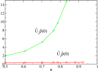
Figure 17: Plots of $\tilde{U}_{s}\tilde{\rho}(0)$ and $\tilde{U}_{c}\tilde{\rho}(0)$ as a function of the filling factor $n$ for $U=6.0$.

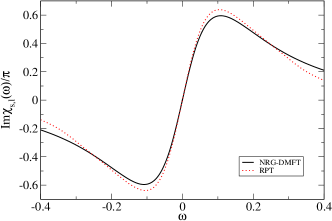
Figure 18: A comparison of imaginary part of the RPT local dynamical spin susceptibility for $U=5.0$, $n=0.942$, with the corresponding NRG-DMFT results

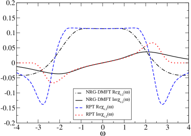
Figure 19: A comparison of imaginary part of the RPT local dynamical charge susceptibility for U=1.5 at half-filling with the corresponding NRG-DMFT results

In Fig. 17 the values of $\tilde{U}_{s}\tilde{\rho}(0)$ and $\tilde{U}_{c}\tilde{\rho}(0)$ are shown away from half-filling as a function of the electron density $n$ for $U=6.0$. The increase of $\tilde{U}_{c}\tilde{\rho}(0)$ as the density increases reflects the lack of phase space for charge fluctuations when $U$ is close to or greater than $U_{c}$. The RPT and NRG-DMFT results for the imaginary part of the local dynamic spin susceptibility for the case $U=5.0$, $n=0.942$ are shown in Fig. 18, and seen to be in good agreement. As the charge susceptibility is heavily suppressed for large value of $U$, NRG-DMFT and RPT results for the real and imaginary parts of the dynamic local charge susceptibility have been calculated for a smaller value of $U$, $U=1.5$, and are compared in Fig. 19. Again over the low energy range there is general agreement in the two sets of results.

VII Calculation of $\chi_{s}({\bf q},\omega)$ and $\chi_{c}({\bf q},\omega)$

Here we discuss briefly the possibility of calculating the ${\bf q}$ and $\omega$ dependent susceptibilities given information about the renormalized quasiparticles. For the previous calculations it was sufficient to know only the local density of states $D(\omega)$ for the lattice and we used the form corresponding to a Bethe lattice. However for the calculation of the $({\bf q},\omega)$ dependent susceptibilities one needs the details of dispersion of the Bloch states $\varepsilon_{\bf k}$. For this type of calculation the Bethe lattice, and even the hypercubic lattice for $d=\infty$, are inappropriate due to their special and restricted ${\bf k}$ dependence (for a discussion of this in detail see the review article of Georges et al. Georges et al. (1996)). However, the DMFT is used as an approximation for calculations in the strong correlation regime for a Hubbard model in three dimensions, and we could consider, for example, an $\varepsilon_{\bf k}$ for a tight-binding cubic lattice. A much used approach for calculating the $({\bf q},\omega)$ spin susceptibility $\chi_{s}({\bf q},\omega)$ is the random phase approximation (RPA), which takes the form,

$$\chi_{s}({\bf q},\omega)={\chi^{0}({\bf q},\omega)\over 1-U\chi^{0}({\bf q},\omega)},$$ (37)

where

$$\chi^{0}({\bf q},\omega)=\sum_{\bf k}{f(\varepsilon({\bf k}+{\bf q}))-f(\varepsilon({\bf k}))\over(\omega-\varepsilon({\bf k}+{\bf q})+\varepsilon({\bf k}))}.$$ (38)

is the dynamic susceptibility of the free electrons. The RPA approximation has been used recently, for example, to estimate the effective electron interaction due to spin fluctuations Hinojosa et al. (2014). This calculation is based on a perturbation expansion in powers of the bare interaction $U$. It is of interest to see how this formula would be modified if the renormalization of the local interaction and of the quasiparticles is taken into account. In the calculation of the dynamical susceptibilities for impurity problems these renormalization effects are found to be very signficantHewson (2006). They can be taken into account by replacing $U$ by $\tilde{U}_{s}$, the renormalized interaction in the spin channel, and the replacing the dynamic susceptibility of the free electrons by the corresponding susceptibility of the free quasiparticles, to give

$$\chi_{s}({\bf q},\omega)={\tilde{\chi}^{0}({\bf q},\omega)\over 1-\tilde{U}_{s}\tilde{\chi}^{0}({\bf q},\omega)},$$ (39)

where

$$\tilde{\chi}^{0}({\bf q},\omega)=\sum_{\bf k}{f(\tilde{\varepsilon}({\bf k}+{\bf q}))-f(\tilde{\varepsilon}({\bf k}))\over(\omega-\tilde{\varepsilon}({\bf k}+{\bf q})+\tilde{\varepsilon}({\bf k}))}.$$ (40)

The renormalized interaction $\tilde{U}_{s}$ is not simply $\tilde{U}$, as the series of diagrams for $\omega=0$ contribute to the 4-vertex at zero frequency, and must be cancelled by the counter term $\lambda_{3}$ so $\tilde{U}_{s}=\tilde{U}-\lambda_{3}$. The counter term $\lambda_{3}$ can be deduced from the calculated static uniform susceptibility $\chi_{s}$ in Eqn. (29) as $\chi_{s}={\rm lim}_{{\bf q}\to 0}{\rm lim}_{{\omega}\to 0}\chi_{s}({\bf q})$. As in the RPA this approximation assumes a local scattering vertex and goes over to the the RPA result in the weak correlation limit as $z\to 1$ and $\tilde{U}_{s}/z\to U$. With this formula, however, we can get enhanced low energy spin fluctations for $\tilde{U}_{s}>0$ arising either close to the onset of a ferromagnetic instability, which requires $\tilde{U}_{s}\tilde{\rho}(0)\geq 1$, where $\tilde{\rho}(0)$ is the value of the quasiparticle density of states at the Fermi level, or close to localization such that $z\ll 1$. As in the RPA, in the case of a tight-binding cubic lattice at half filling, an antiferromagnetic instability is predicted for $\tilde{U}_{s}>0$ and s-wave superconductivity for $\tilde{U}_{s}<0$.

The charge susceptibility $\chi_{c}({\bf q},\omega)$ can be calculated in a similar way,

$$\chi_{c}({\bf q},\omega)={\tilde{\chi}^{0}({\bf q},\omega)\over 1+\tilde{U}_{c}\tilde{\chi}^{0}({\bf q},\omega)},$$ (41)

Note, however, that unlike the standard RPA, the interaction vertex $\tilde{U}_{c}$ is not in general the same as that in the spin channel. A similar approach, with RPA-like forms, with different vertices in the spin and charge channels has been applied by Vilk and TremblayVilk and Tremblay (1997) to the two-dimensional Hubbard model to interpret the results of a Monte Carlo calculation.

VIII Summary

We have shown how information about the low energy quasiparticles can be deduced from an analysis of the low energy fixed point in a DMFT calculation for the Hubbard model, and in particular the on-site renormalized quasiparticle interaction $\tilde{U}$. This information is sufficient to set up a renormalized perturbation expansion for the local self-energy $\Sigma(\omega)$, which is applicable in all parameter regimes. It is particularly useful to be able to derive analytic results in the very strong correlation limit where it is difficult to obtain accurate results from discrete sets of numerical data for the low energy spectra, or where some form of broadening has been applied. We have been able to check some of the analytic expressions in different regimes against the numerical results. We conjecture that there are some universal relations on the approach to the Mott-Hubbard transition such that all the parameters can be expresssed in terms of a single energy scale $T^{*}$ where $T^{*}\to 0$ at the transition.

The calculation of the renormalized parameters has been based on the assumption that the low energy fixed point corresponds to a Fermi liquid. This appears to be the case in all the regimes considered but the quasiparticles disappear on the approach to the Mott-Hubbard transition, so the Fermi liquid expressions are only expected to be valid for temperatures $T$ such that $T\ll T^{*}$. This leaves open the possibility of non-Fermi liquid behavior in the vicinity of the Mott-Hubbard transition, as a quantum critical point, for temperatures such that $T>T^{*}$.

The DMFT approach, with an on-site renormalized vertex $\tilde{U}$, is sufficient to carry out a renormalized perturbation expansion for the self-energy of the infinite dimensional model. The characteristic feature of strongly correlated electron systems is the strong frequency dependence of the self-energy which is taken into account in the DMFT but at the expense of neglecting any wavevector dependence. This is a good initial approximation, taking into account the larger energy scale effects of strong electron correlation, but in three and, particularly two dimensions, the wavevector dependence should be taken into account to examine the more subtle correlation effects that take place on the lowest energy scales. An approach along related lines to that presented here is the dynamical vertex approximationToschi et al. (2007) (D$\Gamma$A), which involves estimates of both the frequency and wavevector dependence of the irreducible 4-vertices. A recent application of this approximation to the Hubbard model is that of Rohringer and ToschiRohringer and Toschi (2016). A simplified feature of the RPT calculation of the low energy response functions on the lowest energy scales is the neglect of the frequency dependence of these renormalized vertices. This gives excellent results, for example, in the strong correlation regime for the Anderson impurity modelHewson (2006). Some estimate of the ${\bf q},\omega$ dependent spin susceptibility, based on a generalized RPA with a local scattering vertex and renormalized parameters derived from a DMFT-NRG calculation, was outlined in section VII. A reasonable approximation going beyond the local approximation could be to take nearest neighbour contributions for the renormalized four-vertex into account, and again neglect any frequency dependence. It is important, however, in using any renormalized vertex that counterterms have to be taken into account to prevent over-counting.

Acknowledgement

We wish to thank Winfried Koller, Dietrich Meyer and Johannes Bauer for their contributions to the development of the NRG used in the calculations, and Sriram Shastry for helpful discussion and comments.

References

- Stewart (1984) G. R. Stewart, Rev. Mod. Phys. 56, 755 (1984).
- Fisk et al. (1995) Z. Fisk, J. L. Sarrao, J. L. Smith, and J. P. Thompson, Proc. Natl. Accd. Sci. USA 92, 663 (1995).
- Coleman et al. (2001) P. Coleman, C. Pepin, Q. Si, and R. Ramazashvili, J. Phys. Condens. Matter 13, R723 (2001).
- Löhneysen et al. (2007) H. Löhneysen, A. Rosch, M. Vojta, and P. Wölfle, Rev. Mod. Phys. 79, 1015 (2007).
- Si and Steglich (2010) Q. Si and F. Steglich, Science 329, 1161 (2010).
- Taillefer (2010) L. Taillefer, Annual Review of Condensed Matter Physics 1, 51 (2010).
- (7) N. Plakida, High-Temperature Cuprate Superconductors: Experiment, Theory and Applications (Springer, 2010).
- Wilson (1975) K. Wilson, Rev. Mod. Phys. 47, 773 (1975).
- Tsvelik and Wiegmann (1983) A. M. Tsvelik and P. B. Wiegmann, Adv. Phys. 32, 453 (1983).
- Andrei et al. (1983) N. Andrei, K. Furuya, and J. H. Lowenstein, Rev. Mod. Phys. 55, 331 (1983).
- Affleck and Ludwig (1993) I. Affleck and A. Ludwig, Phys. Rev. B 48, 7297 (1993).
- Coleman (1984) P. Coleman, Phys. Rev. B 29, 3035 (1984).
- Hewson (1997) A. C. Hewson, The Kondo Problem to Heavy Fermions (Cambridge University Press, Cambridge, 1997).
- Hewson (1993) A. C. Hewson, Phys. Rev. Lett. 70, 4007 (1993).
- Hewson (2006) A. C. Hewson, J. Phys.: Cond. Mat. 18, 1815 (2006).
- Nishikawa et al. (2012a) Y. Nishikawa, D. J. G. Crow, and A. C. Hewson, Phys. Rev. Lett. 108, 056402 (2012a).
- Nishikawa et al. (2012b) Y. Nishikawa, D. J. G. Crow, and A. C. Hewson, Phys. Rev. B 86, 125134 (2012b).
- Hubbard (1963) J. Hubbard, Proc. R. Soc. London, Ser. A 276, 238 (1963).
- Lieb and Wu (1968) E. H. Lieb and F. Wu, Phys. Rev. Lett. 20, 1445 (1968).
- Lieb and Wu (2003) E. H. Lieb and F. Wu, Physica A 321, 1 (2003).
- Haldane (1981) F. D. M. Haldane, J. Phys. C 14, 2585 (1981).
- Bulla et al. (2008) R. Bulla, T. Costi, and T. Pruschke, Rev. Mod. Phys. 80, 395 (2008).
- Jarrell (1992) M. Jarrell, Phys. Rev. Lett. 69, 168 (1992).
- Georges and Krauth (1992) A. Georges and W. Krauth, Phys. Rev. Lett. 69, 1240 (1992).
- Georges et al. (1996) A. Georges, G. Kotliar, W. Krauth, and M. J. Rozenberg, Rev. Mod. Phys. 68, 13 (1996).
- Park et al. (2008) H. Park, K. Haule, and G. Kotliar, Phys. Rev. Lett. 101, 186403 (2008).
- Fuchs et al. (2011) S. Fuchs, E. Gull, M. Troyer, M. Jarrell, and T. Pruschke, Phys. Rev. B 83, 235113 (2011).
- Bauer and Hewson (2007a) J. Bauer and A. C. Hewson, Phys. Rev. B 76, 035118 (2007a).
- Bauer and Hewson (2007b) J. Bauer and A. C. Hewson, Eur. Phys. J. B 57, 235 (2007b).
- Logan and Galpin (2016) D. E. Logan and M. R. Galpin, J. Phys. Condens. Matter 28, 025601 (2016).
- Shastry and Perepelitsky (2016) B. S. Shastry and E. Perepelitsky, Phys. Rev. B 94, 045138 (2016).
- Metzner and Vollhardt (1989) W. Metzner and D. Vollhardt, Phys. Rev. Lett. 62, 324 (1989).
- Müller-Hartmann (1989) E. Müller-Hartmann, Z. Phys. B 74, 507 (1989).
- Luttinger (1960) J. M. Luttinger, Phys. Rev. 119, 1153 (1960).
- Krishna-murthy et al. (1980) H. R. Krishna-murthy, J. W. Wilkins, and K. G. Wilson, Phys. Rev. B 21, 1003 (1980).
- Hewson et al. (2004) A. C. Hewson, A. Oguri, and D. Meyer, Eur. Phys. J. B 40, 177 (2004).
- Bulla (1999) R. Bulla, Phys. Rev. Lett. 83, 136 (1999).
- Luttinger and Ward (1960) J. M. Luttinger and J. C. Ward, Phys. Rev. 118, 1417 (1960).
- Hewson et al. (2006) A. C. Hewson, J. Bauer, and W. Koller, Phys. Rev. B 73, 045117 (2006).
- Kanamori (1963) J. Kanamori, Prog. Theor. Phys 30, 275 (1963).
- Bauer and Hewson (2010) J. Bauer and A. C. Hewson, Phys. Rev. B 81, 235113 (2010).
- Bauer (2009) J. Bauer, Eur. Phys. J. B 68, 201 (2009).
- Pandis and Hewson (2015) V. Pandis and A. C. Hewson, Phys. Rev. B 92, 115131 (2015).
- Zitko et al. (2013) R. Zitko, D. Hansen, E. Perepelitsky, J. Mravlje, A. Georges, and B. S. Shastry, Phys. Rev. B 88, 235132 (2013).
- Hinojosa et al. (2014) A. Hinojosa, A. V. Chubukov, and P. Wölfle, Phys. Rev. B 90, 104509 (2014).
- Vilk and Tremblay (1997) Y. M. Vilk and A. M. S. Tremblay, J. Physique 7, 1309 (1997).
- Toschi et al. (2007) A. Toschi, A. A. Katanin, and K. Held, Phys. Rev. B 75, 045118 (2007).
- Rohringer and Toschi (2016) G. Rohringer and A. Toschi, Phys. Rev. B 94, 125144 (2016).