Abstract

We construct $\mathcal{N}=1$ supersymmetric nonlocal theories in four dimension. We discuss higher derivative extensions of chiral and vector superfields, and write down generic forms of Kähler potential and superpotential up to quadratic order. We derive the condition in which an auxiliary field remains non-dynamical, and the dynamical scalars and fermions are free from the ghost degrees of freedom. We also investigate the nonlocal effects on the supersymmetry breaking and find that supertrace (mass) formula is significantly modified even at the tree level.

1 Introduction

Supersymmetry (SUSY) is perhaps one of the most powerful extensions of physics beyond the standard model, which attempts to unify both spin and charge of a particle by extending the Poincaré group and Lie algebra [1, 2]. It provides an elegant answer to the electroweak hierarchy problem by protecting the Higgs mass, and also provides gauge couplings unification at scales close to the grand unified scale [3].

In this paper we would like to discuss higher derivative extension, especially nonlocal extension, of SUSY. It is generally believed that higher derivative theories can soften the ultraviolet (UV) properties. The propagator for such theories will be more suppressed. However, even at the classical level, the introduction of higher derivative terms in an action is quite dangerous because there is a famous Ostrogradsky theorem [4], which relies on having a momentum associated with higher derivative in the theory in which the energy is seen to be linear, as opposed to quadratic, states that there is a classical instability unless the theory is degenerate [5, 6]. One way is to consider a degenerate theory, in which the momenta associated with higher derivative terms are not invertible. The famous example is Galileon [7]. Supersymmetric extension of those higher derivative theories have been studied recently in [8, 9, 10, 11, 12, 13].

Another way to circumvent Ostrogradsky ghost is to consider infinitely higher derivative theory (nonlocal theory), where no such highest momentum operator can be readily identified, nor there are any extra poles in the propagator which could correspond to new degrees of freedom, such as ghosts or otherwise. Moreover, it has been known that infinite derivatives would definitely improve the ultraviolet properties of the theory. In particular a nonlocal extension of the Einstein gravity has a variety of interesting properties and applications (see, e.g., [14, 15, 16, 17, 18, 19, 20, 21, 22, 23, 24, 25, 26, 27, 28, 29, 30, 31]). It is also known that nonlocal theories capture certain aspects of string theory, particularly in the context of string field theory and p-adic string (see, e.g., [34, 37, 33, 32, 35, 31, 36, 38, 39, 40, 41]). Nonlocal field theories would therefore be useful for constructing and understanding UV complete (gravitational) theories.

Based on such backgrounds, we wish to incorporate SUSY in nonlocal field theories. In this paper we discuss the matter and gauge field sector in particular (see the recent paper [42] for the gravitational sector). Typically, in the off-shell formalism of SUSY construction, an auxiliary field is introduced to balance the degrees of freedom between bosons and fermions. Then, one may wonder what should be the condition we may require in order to keep the auxiliary field non-dynamical, when infinite derivatives are introduced, and how it is related to the condition for the absence of a ghost or tachyons in physical fields.

These important questions must be addressed in order to construct a viable nonlocal SUSY theory. Phenomenologically, it is an interesting question to ask; how the supertrace (mass) formula gets modified. In a global SUSY model, the supertrace (mass) formula vanishes even after the SUSY breaking, albeit radiative corrections slightly modifies it, which implies that not only heavier superpartners but also lighter ones must appear.

In this paper, first of all, we will construct ${\cal N}=1$ infinitely higher derivative extensions of chiral (neutral) superfields up to quadratic orders in four dimensions. We will clarify the condition how to keep the auxiliary field non-dynamical and the absence of ghosts. Then, we extend our construction to vector superfields including charged chiral superfields. Finally, as a simple example of the SUSY breaking, we shall consider a nonlocal extension of O’Raifeartaigh model and discuss how the supertrace formula is modified. Finally, conclusions and discussions will be given.

2 Higher derivative action for chiral superfields

In this section, we would like to introduce a higher derivative extension of the standard SUSY action for chiral superfields. Let us consider,

$$S=\int d^{4}xd^{4}\theta\,K(\Phi_{i},\Phi_{i}^{\dagger},D_{\alpha},\bar{D}_{\dot{\alpha}},\partial_{\mu})+\left[\int d^{4}xd^{2}\theta\,W(\Phi_{i},\Phi_{i}^{\dagger},D_{\alpha},\bar{D}_{\dot{\alpha}},\partial_{\mu})+\text{h.c.}\right]\,,$$ (2.1)

where the Kähler potential $K$, and the superpotential $W$, constructed from $\Phi_{i}$’s, $\Phi_{i}^{\dagger}$’s, and their derivatives are vector and chiral superfields, respectively. This makes the action (2.1) SUSY because super transformations of D-terms and F-terms are total derivatives. In the following we shall construct a higher derivative action of the form (2.1) up to the second order in $\Phi_{i}$ and $\Phi_{i}^{\dagger}$, and introduce a SUSY nonlocal field theory.

2.1 Higher derivative extension of Kähler potential

We begin with the higher derivative extension $K$, of the Kähler potential. Since we just require the reality condition $K^{\dagger}=K$ to preserve SUSY, it is straightforward to write down the concrete form of $K$.

Ingredients for the second order action can be classified into the following two: (1) One contains one chiral and one anti-chiral superfields, and (2) The other contains terms with two chiral superfields and their Hermitian conjugates. A general form of the quadratic action with one chiral superfield, $\Phi_{i}$, and one anti-chiral superfield, $\Phi_{i}^{\dagger}$, is given by

$$\int d^{4}xd^{4}\theta\left[\Phi_{i}\,f_{ij}(\Box)\Phi_{j}^{\dagger}+\text{ h.c. }\right]\,,$$ (2.2)

which can be thought of as a higher derivative extension of kinetic terms. In terms of component fields, it can be written as

$$\int d^{4}xd^{4}\theta\Big{[}\Phi_{i}\,f_{ij}(\Box)\Phi_{j}^{\dagger}+\text{h.c.}\Big{]} =\int d^{4}x\Big{[}\phi_{i}f_{ij}(\Box)\Box\phi_{j}^{*}+F_{i}f_{ij}(\Box)F_{j}^{*}-i\psi_{i}f_{ij}(\Box)\sigma^{\mu}\partial_{\mu}\bar{\psi}_{j}+\text{h.c.}\Big{]}\,,$$ (2.3)

where our notation for component fields is following:

$$\Phi_{i}=\phi_{i}(y)+\sqrt{2}\theta\phi_{i}(y)+\theta^{2}F_{i}(y)\qquad{\rm with}\quad y^{\mu}=x^{\mu}+i\theta\sigma^{\mu}\bar{\theta}\,.$$ (2.4)

Similarly, terms with two chiral superfields and their conjugates are generally of the form:

$$\int d^{4}xd^{4}\theta\Big{[}\Phi_{i}g_{ij}(\Box)D^{2}\Phi_{j}+\text{h.c.}\Big{]} =-4\int d^{4}xd^{2}\theta\,\Big{[}\Phi_{i}g_{ij}(\Box)\Box\Phi_{j}\Big{]}+\text{h.c.}\,.$$ (2.5)

The above term can be thought of as a higher derivative extension of the mass term after integrating by parts. The above equation can be recast in terms of the components, (2.4),

$$\int d^{4}xd^{4}\theta\,\Phi_{i}g_{ij}(\Box)D^{2}\Phi_{j}+\text{h.c.} =-4\int d^{4}x\,\Big{[}\phi_{i}g_{ij}(\Box)\Box F_{j}+F_{i}g_{ij}(\Box)\Box\phi_{j}-\psi_{i}g_{ij}(\Box)\Box\psi_{j}\Big{]}\,.$$ (2.6)

To summarize, the higher derivative extension of the Kähler potential now leads to two types of second order action; higher derivative extension of kinetic term and mass term.

In principle extending our analysis beyond quadratic in superfield to third and higher order will be straightforward, though algebraic calculations become more complicated as we go beyond quadratic order in superfield.

2.2 Higher derivative extension of superpotential

Next we consider higher derivative extension of the superpotential, $W$. Compared to the Kähler potential, the construction of $W$ is rather complicated, because we require the chiral condition $\bar{D}_{\dot{\alpha}}W=0$ to preserve SUSY.

We can solve this condition explicitly at the second order level in $\Phi_{i}$ and $\Phi_{j}^{\dagger}$, and show that all higher derivative terms in the superpotential can be absorbed into the Kähler potential and do not generate new operators.

As a result, a general form of higher derivative quadratic action is given by

$$S =\int d^{4}xd^{4}\theta\Big{[}\Phi_{i}\,f_{ij}(\Box)\Phi_{j}^{\dagger}+\Phi_{i}\,g_{ij}(\Box)D^{2}\Phi_{j}\Big{]}+\int d^{4}xd^{2}\theta\,\bar{m}_{ij}\Phi_{i}\Phi_{j}+\text{h.c.}$$

$$=\int d^{4}xd^{4}\theta\,\Phi_{i}\,f_{ij}(\Box)\Phi_{j}^{\dagger}+\int d^{4}xd^{2}\theta\,\Phi_{i}m_{ij}(\Box)\Phi_{j}+\text{h.c.}\,,$$ (2.7)

where $m_{ij}(\Box)=-4g_{ij}(\Box)\Box+\bar{m}_{ij}$ can be thought of as the higher derivative extension of the mass term.

2.3 Second order action and physical spectra

We now discuss the physical spectrum of higher derivative quadratic action in the following generic form:

$$S_{2} =\int d^{4}xd^{4}\theta\,\Phi_{i}f_{i}(\Box)\Phi_{i}^{\dagger}+\left[\int d^{4}xd^{2}\theta\,\Phi_{i}m_{ij}(\Box)\Phi_{j}+\text{h.c.}\right]\,,$$ (2.8)

where $f_{i}$’s are real functions of d’Alembertian and $m_{ij}$’s are complex symmetric functions $m_{ij}=m_{ji}$.

Also note that we diagonalized the (higher derivative extension of) kinetic terms. In terms of component fields, it can be written as

$$S_{2} =\int d^{4}x\,\Big{[}\phi_{i}\,f_{i}(\Box)\Box\phi_{i}^{*}+F_{i}\,f_{i}(\Box)F_{i}^{*}-i\psi_{i}f_{i}(\Box)\sigma^{\mu}\partial_{\mu}\bar{\psi}_{i}$$

$$\qquad\qquad+\Big{(}\phi_{i}m_{ij}(\Box)F_{j}-\frac{1}{2}\psi_{i}m_{ij}(\Box)\psi_{j}+\text{h.c.}\Big{)}\Big{]}\,.$$ (2.9)

An important point here is that the auxiliary fields, $F_{i}$’s, acquire the kinetic term for a general choice of $f_{i}$’s. The scalars, $\phi_{i}$’s, and the fermions, $\psi_{i}$’s, also obtain additional dynamical degrees of freedom in general.

2.4 Dynamical degrees of freedom

Now, we need to understand the true dynamical degrees of freedom - in order to clarify under what conditions dynamical degrees of freedom would be the same as that of the standard local theory, in the limit when $f_{i}(\Box)\rightarrow 1$, we need to first complete the square with respect to $F_{i}$’s:

$$S_{2}=\int d^{4}x\,\Big{[}\phi_{i}\,f_{i}(\Box)\Box\phi_{i}^{*}-\phi_{j}m_{ij}(\Box)\,f_{i}(\Box)^{-1}m_{ik}^{*}(\Box)\phi_{k}^{*}$$

$$\qquad\qquad\qquad-i\psi_{i}f_{i}(\Box)\sigma^{\mu}\partial_{\mu}\bar{\psi}_{i}-\frac{1}{2}\left(\psi_{i}m_{ij}(\Box)\psi_{j}+\text{h.c.}\right)$$

$$\qquad\qquad\qquad+\left(F_{i}+f_{i}(\Box)^{-1}m^{*}_{ij}(\Box)\phi^{*}_{j}\right)\,f_{i}(\Box)\left(F_{i}^{*}+f_{i}(\Box)^{-1}m_{ik}(\Box)\phi_{k}\right)\Big{]}\,.$$ (2.10)

Note that in order to keep $F_{i}$’s auxiliary, or non-dynamical fields, $f_{i}(\Box)$’s must have no zeros, equivalently, $f_{i}^{-1}(\Box)$’s must have no poles. It should be noticed that, at this stage, the positivity of $f_{i}(\Box)$’s is not necessarily required.

For simplicity, let us assume that $m_{ij}(\Box)$ is diagonal and real: $m_{ij}(\Box)=\delta_{ij}m_{i}(\Box)$ and $m_{i}(\Box)^{*}=m_{i}(\Box)$. The action after integrating out the auxiliary fields $F_{i}$’s is then given by:

$$S_{2} =\int d^{4}x\Big{[}\phi_{i}\,f_{i}(\Box)\left(\Box+f_{i}(\Box)^{-2}m_{i}(\Box)^{2}\right)\phi_{i}^{*}$$

$$\qquad\qquad-i\psi_{i}f_{i}(\Box)\sigma^{\mu}\partial_{\mu}\bar{\psi}_{i}-\Big{(}\frac{1}{2}\psi_{i}m_{i}(\Box)\psi_{j}+\text{h.c.}\Big{)}\Big{]}\,.$$ (2.11)

The on-shell conditions for $\phi_{i}$ and $\psi_{i}$ are then given by the equation of motion:

$$f_{i}(\Box)\left(\Box+f_{i}(\Box)^{-2}m_{i}(\Box)^{2}\right)\phi_{i}=0\,,$$

$$f_{i}(\Box)^{2}\left(\Box+f_{i}(\Box)^{-2}m_{i}(\Box)^{2}\right)\psi_{i}=0\,.$$ (2.12)

Here, we would like to discuss the true dynamical degrees of freedom participating in any classical dynamics. Now, if we demand that this infinite derivative theory maintains the original degrees of freedom corresponding to that of a local $2$-derivative theory, then we need the following conditions:

• $f_{i}(\Box)$’s must not contain any zeroes: This is required in order to maintain $F_{i}$’s non-dynamical degrees of freedom.

• At most $1$-zero from $\left(\Box+f_{i}(\Box)^{-2}m_{i}(\Box)^{2}\right)$: Since $f_{i}(\Box)$’s do not contain any zero, therefore $\left(\Box+f_{i}(\Box)^{-2}m_{i}(\Box)^{2}\right)=0$ should have only one solution for the $\Box$. All of the other cases lead to additional degree of freedom.

• $f_{i}(\Box)>0$: In addition, if we require that this dynamical degree of freedom has healthy kinetic term (that is, correct signature), $f_{i}(\Box)$’s must be positive. Otherwise, this dynamical degree of freedom itself becomes ghost.

These conditions are satisfied only when $f_{i}(\Box)$’s (or equivalently $f_{i}^{-1}(\Box)$’s) is exponential of an entire function, i.e. $e^{-\gamma(\Box)}$, where $\gamma(\Box)$ is an entire function, such a function does not introduce any pole in the complex plane. For $\gamma>0$, as $\Box\rightarrow\infty$, it is easy to see why the propagator is even more convergent in the UV.

In our case, one simple choice which would reproduce the original local spectrum could be $m_{i}(\Box)=\bar{m}_{i}f_{i}(\Box)$ with $\bar{m}_{i}$ being the mass in the local theory, and $f_{i}(\Box)\sim e^{-\gamma(\Box)}$.

3 Introducing gauge sector

In this section we will introduce a vector superfield by gauging the covariant derivatives.

3.1 Gauge covariant derivatives

Let us consider an Abelian gauge symmetry, an extension to non-Abelian case will be straightforward. We will define general superfields with the charge $(p,q)$ by the following transformation rule,

$$\mathcal{O}_{p,q}\to\mathcal{O}^{\prime}_{p,q}=e^{ip\Lambda}e^{-iq\Lambda^{\dagger}}\mathcal{O}_{p,q}\,.$$ (3.1)

Note that the complex conjugate of the operator $\mathcal{O}_{p,q}$ has a charge $(q,p)$ in our convention. The gauge covariant extension of the spinorial derivatives, $D_{\alpha}$ and $\bar{D}_{\dot{\alpha}}$, is then defined by

$$\mathcal{D}_{\alpha}\mathcal{O}_{p,q}=D_{\alpha}\mathcal{O}_{p,q}+p\left(D_{\alpha}V\right)\mathcal{O}_{p,q}\,,$$ (3.2)

$$\bar{\mathcal{D}}_{\dot{\alpha}}\mathcal{O}_{p,q}=\bar{D}_{\dot{\alpha}}\mathcal{O}_{p,q}+q\left(\bar{D}_{\dot{\alpha}}V\right)\mathcal{O}_{p,q}\,,$$ (3.3)

where the vector superfield, $V$, transforms as $V\to V+i\left(\Lambda^{\dagger}-\Lambda\right)$. We also introduce the vectorial gauge covariant derivative, as

$$\mathcal{D}_{\mu}\mathcal{O}_{p,q}\ =\ -\frac{i}{4}\bar{\sigma}{}_{\mu}^{\dot{\alpha}\alpha}\{\mathcal{D}_{\alpha},\bar{\mathcal{D}}_{\dot{\alpha}}\}\mathcal{O}_{p,q}\ =\ \partial_{\mu}\mathcal{O}_{p,q}+pB_{\mu}\mathcal{O}_{p,q}+q\tilde{B}_{\mu}\mathcal{O}_{p,q}\,,$$ (3.4)

where $B_{\mu}$ and $\bar{B}_{\mu}$ are defined by

$$B_{\mu}=-\frac{i}{4}\bar{\sigma}{}_{\mu}^{\dot{\alpha}\alpha}\left(\bar{D}_{\dot{\alpha}}D_{\alpha}V\right)\,,\quad\tilde{B}_{\mu}=-\frac{i}{4}\bar{\sigma}{}_{\mu}^{\dot{\alpha}\alpha}\left(D_{\alpha}\bar{D}_{\dot{\alpha}}V\right)\,,$$ (3.5)

with the following gauge transformations,

$$B_{\mu}\to B_{\mu}-i\partial_{\mu}\Lambda\,,\quad\tilde{B}_{\mu}\to\tilde{B}_{\mu}+i\partial_{\mu}\Lambda^{\dagger}\,.$$ (3.6)

It should be noticed that the vector covariant derivative, $\mathcal{D}_{\mu}$, does not commute with $\mathcal{D}_{\alpha}$, and $\mathcal{D}_{\dot{\alpha}}$, which suggest that the vector covariant derivative of chiral superfields do not satisfy the chirality condition:

$$\left[\bar{D}_{\dot{\alpha}},\mathcal{D}_{\mu}\right]\Phi=q\left(\bar{D}_{\dot{\alpha}}B_{\mu}\right)\Phi=\frac{i}{2}qW^{\alpha}\sigma_{\mu\alpha\dot{\alpha}}\Phi\,,$$ (3.7)

where $W_{\alpha}$ is the gauge invariant field strength, defined later.

It is then straightforward to gauge covariantize the matter sector by using the covariant derivatives introduced above. For example, the general quadratic action (2.8) for the chiral superfields $\Phi_{1}$ and $\Phi_{2}$ with the charges $(1,0)$ and $(-1,0)$, respectively, is simply covariantized as

$$S =\int d^{4}xd^{4}\theta\,\Big{[}\Phi_{1}^{\dagger}\,e^{+gV}f_{1}(\mathcal{D}_{\mu}^{2})\Phi_{1}+\Phi_{2}^{\dagger}\,e^{-gV}f_{2}(\mathcal{D}_{\mu}^{2})\Phi_{2}\Big{]}$$

$$\quad+\int d^{4}xd^{2}\theta\,\Phi_{1}\bar{D}_{\dot{\alpha}}\bar{D}^{\dot{\alpha}}\mathcal{D}^{\alpha}\mathcal{D}_{\alpha}g(\mathcal{D}_{\mu}^{2})\Phi_{2}+\text{h.c.}\,,$$ (3.8)

up to terms with field strengths. We should note that the covariantization of a given matter theory is not unique, because we may always add terms with field strengths such as $(\partial_{\mu}B_{\nu}-\partial_{\nu}B_{\mu})^{2}\Phi^{\dagger}\Phi$ and $W_{\alpha}^{2}\Phi^{2}$. The extensions of the matter sector are summarized in Table 3.1.

${\begin{array}[]{c||c|c|c}\hline\cr&\text{canonical}&\text{second order}&\text{higher order}\\ \hline\cr\hline\cr\hbox{\multirowsetup neutral}&\big{[}\Phi_{i}^{\dagger}\Phi_{i}\big{]}_{\text{D}}&\big{[}\Phi_{i}^{\dagger}\Box\Phi_{i}\big{]}_{\text{D}}&\big{[}\Phi_{i}^{\dagger}f_{ij}(\Box)\Phi_{j}\big{]}_{\text{D}}\\ &\big{[}\Phi_{i}\Phi_{j}\big{]}_{\text{D}}&\big{[}\Phi_{i}D_{\alpha}^{2}\Phi_{j}\big{]}_{\text{D}}\simeq\big{[}\Phi_{i}\Box\Phi_{j}\big{]}_{\text{F}}&\big{[}\Phi_{i}\Box g_{ij}(\Box)\Phi_{j}\big{]}_{\text{F}}\\ \hline\cr\hbox{\multirowsetup charged}&\big{[}|\Phi_{1}|^{2}\,e^{+gV}\big{]}_{\text{D}}&\big{[}\Phi_{1}^{\dagger}\,e^{+gV}{\cal D}_{\mu}^{2}\Phi_{1}\big{]}_{\text{D}}&\big{[}\Phi_{1}^{\dagger}\,e^{+gV}f_{1}({\cal D}_{\mu}^{2})\Phi_{1}\big{]}_{\text{D}}\\ &\big{[}|\Phi_{2}|^{2}\,e^{-gV}\big{]}_{\text{D}}&\big{[}\Phi_{2}^{\dagger}\,e^{-gV}{\cal D}_{\mu}^{2}\Phi_{2}\big{]}_{\text{D}}&\big{[}\Phi_{2}^{\dagger}\,e^{-gV}f_{2}({\cal D}_{\mu}^{2})\Phi_{2}\big{]}_{\text{D}}\\ &\big{[}\Phi_{1}\Phi_{2}\big{]}_{\text{D}}&\big{[}\Phi_{1}{\cal D}_{\alpha}^{2}\Phi_{2}\big{]}_{\text{D}}\simeq\big{[}\Phi_{1}\bar{D}{}_{\dot{\alpha}}^{2}{\cal D}_{\alpha}^{2}\Phi_{2}\big{]}_{\text{F}}&\big{[}\Phi_{1}\bar{D}{}_{\dot{\alpha}}^{2}{\cal D}_{\alpha}^{2}\,g({\cal D}_{\mu}^{2})\Phi_{2}\big{]}_{\text{F}}\\ \hline\cr\end{array}}$

Table table: Higher derivative extensions of the quadratics of the neutral and charged chiral superfields in the superfield formalism. Here $[\ldots]_{\text{D}}$ and $[\ldots]_{\text{F}}$ are abbreviation of the integral $\int d^{4}\theta$ and $\int d^{2}\theta$, respectively. Also $\simeq$ here implies that the both sides are the same up to total derivative terms and an overall coefficient.

The first column implies the chiral superfields $\Phi_{i}$ are neutral or charged under the gauge symmetry. In the second column the canonical term in each chiral superfield is described. The third column gives a certain extension of each canonical term involving the second order derivatives. In the fourth column the terms involves higher order derivatives provided by the functions $f_{ij}(\Box)$ and $g_{ij}(\Box)$ for the neutral chiral superfields, and $f_{1}({\cal D}_{\mu}^{2})$, $f_{2}({\cal D}_{\mu}^{2})$, and $g({\cal D}_{\mu}^{2})$ for the charged chiral superfields. Under a theoretical constraint such as anomaly free, there exists a certain relation among their functions. We emphasize that $\bar{D}{}_{\dot{\alpha}}^{2}$ in $[\ldots]_{\text{F}}$ is the chiral projection operator acting on a non-chiral operator ${\cal D}_{\alpha}^{2}\Phi_{i}$.

3.2 Gauge sector

We now briefly discuss the gauge field. The field strength is encoded in gauge invariant superfields, defined by

$$W_{\alpha}=-\frac{1}{4}\bar{D}^{2}D_{\alpha}V\,,\quad\bar{W}_{\dot{\alpha}}=-\frac{1}{4}D^{2}\bar{D}_{\dot{\alpha}}V\,.$$ (3.9)

Since $W_{\alpha}$ and $\bar{W}_{\dot{\alpha}}$ are chiral and antichiral superfields, respectively. We can show that a general quadratic action constructed from $W_{\alpha}$ and $\bar{W}_{\dot{\alpha}}$ is given by

$$S_{W} =\frac{1}{4}\left[\int d^{4}xd^{2}\theta\,W^{\alpha}g(\Box)W_{\alpha}+\text{h.c.}\right]\,.$$ (3.10)

Note that $\int d^{4}xd^{4}\theta\,W^{\alpha}\sigma^{\mu}_{\alpha\dot{\alpha}}f(\Box)\partial_{\mu}\bar{W}^{\dot{\alpha}}$ and higher derivative extensions of the Fayet-Iliopolous (FI) term are total derivatives.

4 Infinite derivative extension of O’Raifeartaigh model

Before we conclude, let us discuss briefly an infinite derivative extension of the O’Raifeartaigh model, where we shall discuss how the mass formula get modified.

Let us begin with the following action:

$$S =\int d^{4}xd^{4}\theta\,\Phi_{i}f_{i}(\Box)\Phi_{i}^{\dagger}+\left[\int d^{4}xd^{2}\theta\,\Phi_{1}m(\Box)\Phi_{2}+\lambda\Phi_{0}+g\Phi_{0}\Phi_{1}\Phi_{1}+\text{h.c.}\right]\,.$$ (4.1)

For the moment, we leave $f_{i}(\Box)$ and $m(\Box)$ as arbitrary functions of d’Alembertian satisfying $f_{i}(0)=1$ and $m(0)=m$, in order to reach the local limit in the IR. Note that we keep the cubic interactions local for simplicity. Also there are no derivative terms for linear terms because they are total derivatives. In terms of component fields, the action is given by:

$$S =\int\!d^{4}x\bigg{[}\sum_{i}\left(\phi_{i}f_{i}(\Box)\Box\phi_{i}^{*}+F_{i}f_{i}(\Box)F_{i}^{*}-i\psi_{i}f_{i}(\Box)\sigma^{\mu}\partial_{\mu}\bar{\psi}_{i}\right)$$

$$\qquad\qquad+\left[\lambda F_{0}+\left(F_{1}m(\Box)\phi_{2}+F_{2}m(\Box)\phi_{1}-\psi_{1}m(\Box)\psi_{2}\right)\right.$$

$$\qquad\qquad\left.+g\left(F_{0}\phi_{1}^{2}+2F_{1}\phi_{0}\phi_{1}-\psi_{1}\psi_{1}\phi_{0}-2\psi_{0}\psi_{1}\phi_{1}\right)\right]+\text{h.c.}\bigg{]}\,.$$ (4.2)

By integrating out the auxiliary fields $F_{i}$, we obtain the action of the form:

$$S =\int d^{4}x\bigg{[}\sum_{i}\left(\phi_{i}f_{i}(\Box)\Box\phi_{i}^{*}-i\psi_{i}f_{i}(\Box)\sigma^{\mu}\partial_{\mu}\bar{\psi}_{i}\right)$$

$$\qquad\qquad-\psi_{1}m(\Box)\psi_{2}-\bar{\psi}_{1}m(\Box)\bar{\psi}_{2}-\lambda-\lambda g(\phi_{1}^{2}+\phi_{1}^{*2})$$

$$\qquad\qquad-\phi_{2}f_{1}(\Box)^{-1}m(\Box)^{2}\phi_{2}^{*}-\phi_{1}f_{2}(\Box)^{-1}m(\Box)^{2}\phi_{1}^{*}+\ldots\bigg{]}\,,$$ (4.3)

where the dots stand for cubic and quartic terms in $\phi_{i}$. Since homogeneous equations of motion are the same as that of the original (local) O’Raifeartaigh model, in our case, we obtain two classes of vacua, which we shall discuss below.

Here let us consider the spectrum around the vacuum $\phi_{0}=\phi_{1}=\phi_{2}=0$. The on-shell condition for $\phi_{0}$ and $\psi_{0}$ is given by

$$f_{0}(\Box)^{2}\Box=0\,,$$ (4.4)

and that for $\psi_{1}$, $\psi_{2}$, and $\phi_{2}$ is given by

$$f_{1}(\Box)f_{2}(\Box)\Box-m(\Box)^{2}=0\,.$$ (4.5)

On the other hand, the $\phi_{1}$ sector is modified by the $\lambda$ interaction, as

$$f_{1}(\Box)f_{2}(\Box)\Box-\left(m(\Box)^{2}\pm 2\lambda g\right)=0\,,$$ (4.6)

where the plus/minus sign is for the real/imaginary part of $\phi_{1}$. Let us then choose $f_{i}(\Box)$ and $m(\Box)$ as the following Gaussian operator

$$f_{i}(\Box)=m(\Box)=e^{-\Box/M^{2}}\,,$$ (4.7)

where we have explicitly introduced the scale of nonlocality, $M$. If we decompose $\phi_{1}$ into the real and the imaginary part, as $\phi_{1}=\frac{1}{\sqrt{2}}(\pi+i\sigma)$, the masses of $\pi$ and $\sigma$ are affected by the nonlocality. The on-shell conditions then give;

$$e^{-\Box/M^{2}}(\Box-m^{2})=\pm 2\lambda g\,,$$ (4.8)

and if we introduce a dimensionless parameter $x=\Box/M^{2}$, the above equation can be expressed as

$$e^{-x}\left(x-\frac{m^{2}}{M^{2}}\right)=\pm\frac{2\lambda g}{M^{2}}\,.$$ (4.9)

Plotting the behavior of (4.9) in Figure 4, we can read off a couple of interesting phenomena.

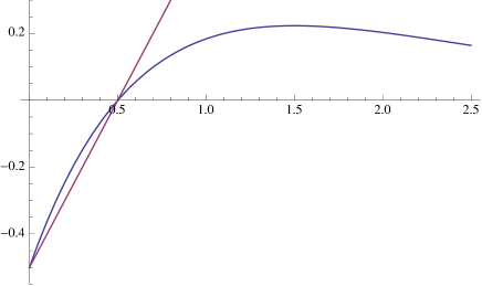
Figure figure: The straight line denotes $(x-\frac{m^{2}}{M^{2}})$ without any nonlocality, while the curved line indicates the operator $e^{-x}(x-\frac{m^{2}}{M^{2}})$ in (4.9) which involves the nonlocal effect by the factor $e^{-x}$. Here we set $m^{2}/M^{2}=0.5$.

In this figure, a numerical value of $2\lambda g/M^{2}$ in the right-hand side of (4.9) is represented as a horizontal line. It turns out that the propagator of $\pi$ does not have a physical pole for $2\lambda g/M^{2}\gtrsim 0.22$. This is because the horizontal line expressing $2\lambda g/M^{2}$ does not cross the curved line beyond that value. In other words there does not exist a solution of (4.9). This situation is analogous to the open string tachyon condensation in the level truncated theory (see, e.g., [45]).

If $2\lambda g/M^{2}$ takes a value $0<2\lambda g/M^{2}\lesssim 0.22$, the horizontal line cross the curved line at two points. This means that $\pi$ has two poles. However, one of the poles has a wrong sign, i.e., the pole gives rise to the negative norm and it provides an unphysical mode. Such a parameter region should be avoided in order for our simple nonlocal model to be trustable at the UV scale. We would like to emphasize that such a dangerous signal appears even at the tree-level.

On the other hand, the situation for $\sigma$ is not so different from the local case (when $2\lambda g>0$). Furthermore, in the limit $M\rightarrow\infty$, the mass formula reduces to that of the local case.

5 Conclusions and discussions

In this paper, we have constructed $\mathcal{N}=1$ supersymmetric nonlocal theories in four dimension. We discuss higher derivative extensions of chiral and vector superfields, and write down generic forms of Kähler potential and superpotential up to quadratic order. We find that there are only nonlocal extensions of the standard canonical kinetic term and the mass term. Based on this action, we derive the condition for (neutral) chiral superfields in which an auxiliary field remains non-dynamical, and find that the same condition is necessary to remove the ghost degree of freedom from dynamical fields. The extension to charged chiral fields are straightforward and the complete treatment will be discussed in the future publication [46]. We have also investigated the nonlocal effects on the supersymmetry breaking. As a concrete example, a nonlocal extension of O’Raiferataigh model is discussed. The on-shell condition for each field is derived and we find that that supertrace (mass) formula is significantly modified even at the tree level, which has interesting implications on collider physics and cosmology.

References

- [1] Y. A. Golfand and E. P. Likhtman, “Extension of the algebra of Poincaré group generators and violation of invariance,” JETP Lett. 13 (1971) 323 [Pisma Zh. Eksp. Teor. Fiz. 13 (1971) 452].
- [2] R. Haag, J. T. Lopuszanski and M. Sohnius, “All possible generators of supersymmetries of the -matrix,” Nucl. Phys. B 88 (1975) 257.
- [3] S. P. Martin, “A supersymmetry primer,” Adv. Ser. Direct. High Energy Phys. 21 (2010) 1 [Adv. Ser. Direct. High Energy Phys. 18 (1998) 1] [hep-ph/9709356].
- [4] M. Ostrogradsky, “Memoires sur les equations differentielles, relatives au probleme des isoperimetres,” Mem. Acad. St. Petersbourg 6 (1850) 385.
- [5] R. P. Woodard, “Avoiding dark energy with modifications of gravity,” Lect. Notes Phys. 720 (2007) 403 [astro-ph/0601672].
- [6] R. P. Woodard, “Ostrogradsky’s theorem on Hamiltonian instability,” Scholarpedia 10 (2015) 32243 [arXiv:1506.02210 [hep-th]].
- [7] A. Nicolis, R. Rattazzi and E. Trincherini, “The Galileon as a local modification of gravity,” Phys. Rev. D 79 (2009) 064036 [arXiv:0811.2197 [hep-th]].
- [8] J. Khoury, J. L. Lehners and B. Ovrut, “Supersymmetric and the ghost condensate,” Phys. Rev. D 83 (2011) 125031 [arXiv:1012.3748 [hep-th]].
- [9] F. S. Gama, M. Gomes, J. R. Nascimento, A. Y. Petrov and A. J. da Silva, “On the higher-derivative supersymmetric gauge theory,” Phys. Rev. D 84 (2011) 045001 [arXiv:1101.0724 [hep-th]].
- [10] J. Khoury, J. L. Lehners and B. A. Ovrut, “Supersymmetric Galileons,” Phys. Rev. D 84 (2011) 043521 [arXiv:1103.0003 [hep-th]].
- [11] M. Nitta and S. Sasaki, “Higher derivative corrections to manifestly supersymmetric nonlinear realizations,” Phys. Rev. D 90 (2014) 105002 [arXiv:1408.4210 [hep-th]].
- [12] A. Addazi and G. Esposito, “Nonlocal quantum field theory without acausality and nonunitarity at quantum level: is SUSY the key?,” Int. J. Mod. Phys. A 30 (2015) 1550103 [arXiv:1502.01471 [hep-th]].
- [13] S. Aoki and Y. Yamada, “Impacts of supersymmetric higher derivative terms on inflation models in supergravity,” JCAP 1507 (2015) 020 [arXiv:1504.07023 [hep-th]].
- [14] A. Pais and G. E. Uhlenbeck, “On field theories with nonlocalized action,” Phys. Rev. 79 (1950) 145.
- [15] K. S. Stelle, “Renormalization of higher derivative quantum gravity,” Phys. Rev. D 16 (1977) 953.
- [16] E. Tomboulis, “Renormalizability and asymptotic freedom in quantum gravity,” Phys. Lett. B 97 (1980) 77.
- [17] E. T. Tomboulis, “Renormalization and asymptotic freedom In quantum gravity,” In *Christensen, S.m. ( Ed.): Quantum Theory Of Gravity*, 251-266 and Preprint - TOMBOULIS, E.T. (REC.MAR.83) 27p.
- [18] J. W. Moffat, “Finite nonlocal gauge field theory,” Phys. Rev. D 41 (1990) 1177.
- [19] E. T. Tomboulis, “Superrenormalizable gauge and gravitational theories,” hep-th/9702146.
- [20] T. Biswas, A. Mazumdar and W. Siegel, “Bouncing universes in string-inspired gravity,” JCAP 0603 (2006) 009 [hep-th/0508194].
- [21] N. Barnaby and N. Kamran, “Dynamics with infinitely many derivatives: the initial value problem,” JHEP 0802 (2008) 008 [arXiv:0709.3968 [hep-th]].
- [22] N. Barnaby and N. Kamran, “Dynamics with infinitely many derivatives: variable coefficient equations,” JHEP 0812 (2008) 022 [arXiv:0809.4513 [hep-th]].
- [23] L. Modesto, “Super-renormalizable quantum gravity,” Phys. Rev. D 86 (2012) 044005 [arXiv:1107.2403 [hep-th]].
- [24] T. Biswas, E. Gerwick, T. Koivisto and A. Mazumdar, “Towards singularity and ghost free theories of gravity,” Phys. Rev. Lett. 108 (2012) 031101 [arXiv:1110.5249 [gr-qc]].
- [25] T. Biswas and N. Okada, “Towards LHC physics with nonlocal Standard Model,” Nucl. Phys. B 898 (2015) 113 [arXiv:1407.3331 [hep-ph]].
- [26] S. Talaganis, T. Biswas and A. Mazumdar, “Towards understanding the ultraviolet behavior of quantum loops in infinite-derivative theories of gravity,” Class. Quant. Grav. 32 (2015) 215017 [arXiv:1412.3467 [hep-th]].
- [27] E. T. Tomboulis, “Nonlocal and quasilocal field theories,” Phys. Rev. D 92 (2015) 125037 [arXiv:1507.00981 [hep-th]].
- [28] T. Biswas, A. S. Koshelev and A. Mazumdar, “Consistent higher derivative gravitational theories with stable de Sitter and anti-de Sitter backgrounds,” arXiv:1606.01250 [gr-qc].
- [29] T. Biswas, A. S. Koshelev and A. Mazumdar, “Gravitational theories with stable (anti-)de Sitter backgrounds,” Fundam. Theor. Phys. 183 (2016) 97 [arXiv:1602.08475 [hep-th]].
- [30] S. Talaganis and A. Mazumdar, “High-energy scatterings in infinite-derivative field theory and ghost-free gravity,” Class. Quant. Grav. 33 (2016) 145005 [arXiv:1603.03440 [hep-th]].
- [31] R. Pius and A. Sen, “Cutkosky Rules for Superstring Field Theory,” arXiv:1604.01783 [hep-th].
- [32] K. Ohmori, “A Review on tachyon condensation in open string field theories,” hep-th/0102085.
- [33] W. Taylor and B. Zwiebach, “D-branes, tachyons, and string field theory,” hep-th/0311017.
- [34] Y. Okawa, “Analytic methods in open string field theory,” Prog. Theor. Phys. 128 (2012) 1001.
- [35] N. Moeller and B. Zwiebach, “Dynamics with infinitely many time derivatives and rolling tachyons,” JHEP 0210 (2002) 034 [hep-th/0207107].
- [36] P. G. O. Freund and M. Olson, “Nonarchimedean strings,” Phys. Lett. B 199 (1987) 186.
- [37] G. Calcagni and L. Modesto, “Nonlocality in string theory,” J. Phys. A 47 (2014) 355402 [arXiv:1310.4957 [hep-th]].
- [38] P. G. O. Freund and E. Witten, “Adelic string amplitudes,” Phys. Lett. B 199 (1987) 191.
- [39] L. Brekke, P. G. O. Freund, M. Olson and E. Witten, “Nonarchimedean string dynamics,” Nucl. Phys. B 302 (1988) 365.
- [40] D. Ghoshal and A. Sen, “Tachyon condensation and brane descent relations in p-adic string theory,” Nucl. Phys. B 584 (2000) 300 [hep-th/0003278].
- [41] J. A. Minahan, “Quantum corrections in p-adic string theory,” hep-th/0105312.
- [42] S. Giaccari and L. Modesto, “Classical and Quantum Nonlocal Supergravity,” arXiv:1605.03906 [hep-th].
- [43] J. Wess and J. Bagger, “SUSY and supergravity,” Princeton, USA: Univ. Pr. (1992) 259 p.
- [44] J. Edholm, A. S. Koshelev and A. Mazumdar, “Universality of testing ghost-free gravity,” arXiv:1604.01989 [gr-qc].
- [45] I. Ellwood and W. Taylor, “Open string field theory without open strings,” Phys. Lett. B 512 (2001) 181 [hep-th/0103085].
- [46] T. Kimura, A. Mazumdar, T. Noumi, and M. Yamaguchi, in preparation.