Sharp local boundedness and maximum principle in the infinitely degenerate regime via DeGiorgi iteration

Abstract.

We obtain local boundedness and maximum principles for weak subsolutions to certain infinitely degenerate elliptic divergence form inhomogeneous equations. For example, we consider the family $\left\{f_{\sigma}\right\}_{\sigma>0}$ with

$$f_{\sigma}\left(x\right)=e^{-\left(\frac{1}{\left|x\right|}\right)^{\sigma}},\ \ \ \ \ -\infty<x<\infty,$$

of infinitely degenerate functions at the origin, and show that all weak solutions to the associated infinitely degenerate quasilinear equations of the form

$$\mathop{\mathrm{d}iv}A\left(x,u\right)\mathop{\mathrm{g}rad}u=\phi\left(x\right),\ \ \ A\left(x,z\right)\sim\left[\begin{array}[]{cc}I_{n-1}&0\\ 0&f\left(x_{1}\right)^{2}\end{array}\right],$$

with rough data $A$ and $\phi$, are locally bounded for admissible $\phi$ provided $0<\sigma<1$. We also show that these conditions are necessary for local boundedness in dimension $n\geq 3$, thus paralleling the known theory for the smooth Kusuoka-Strook operators $\frac{\partial^{2}}{\partial x_{1}^{2}}+\frac{\partial^{2}}{\partial x_{2}^{2}}+f_{\sigma}\left(x\right)^{2}\frac{\partial^{2}}{\partial x_{3}^{2}}$. We also show that subsolutions satisfy a maximum principle for admissible $\phi$ under the same restriction on the degeneracy.

In order to prove these theorems, we first establish abstract results in which certain Poincaré and Orlicz Sobolev inequalities are assumed to hold. We then develop subrepresentation inequalities for control geometries in order to obtain the needed Poincaré and Orlicz Sobolev inequalities.

Preface

There is a large and well-developed theory of elliptic and subelliptic equations with rough data, beginning with work of DeGiorgi-Nash-Moser, and also a smaller theory still in its infancy of infinitely degenerate elliptic equations with smooth data, beginning with work of Fedii and Kusuoka-Strook, and continued by Morimoto and Christ. Our purpose here is to initiate a study of the DeGiorgi regularity theory, as presented by Caffarelli-Vasseur, in the context of equations that are both infinitely degenerate elliptic and have rough data. This monograph can be viewed as taking the first steps in such an investigation and more specifically, in identifying a number of surprises encountered in the implementation of DeGiorgi iteration in the infinitely degenerate regime. The similar approach of Moser in the infinitely degenerate regime is initiated in our paper [KoRiSaSh1], but is both technially more complicated and more demanding of the underlying geometry. As a consequence, the results in [KoRiSaSh1] for local boundedness are considerably weaker than the sharp results obtained here with the DeGiorgi approach. On the other hand, the method of Moser does apply to obtain continuity for solutions to inhomogeneous equations, but at the expense of a much more elaborate proof strategy. The parallel approach of Nash seems difficult to adapt to the infinitely degenerate case, but remains a possibility for future research.

Part I Overview

The regularity theory of subelliptic linear equations with smooth coefficients is well established, as evidenced by the results of Hörmander [Ho] and Fefferman and Phong [FePh]. In [Ho], Hörmander obtained hypoellipticity of sums of squares of smooth vector fields whose Lie algebra spans at every point. In [FePh], Fefferman and Phong considered general nonnegative semidefinite smooth linear operators, and characterized subellipticity in terms of a containment condition involving Euclidean balls and ”subunit” balls related to the geometry of the nonnegative semidefinite form associated to the operator.

The theory in the infinite regime however, has only had its surface scratched so far, as evidenced by the results of Fedii [Fe] and Kusuoka and Strook [KuStr]. In [Fe], Fedii proved that the two-dimensional operator $\frac{\partial}{\partial x^{2}}+f\left(x\right)^{2}\frac{\partial}{\partial y^{2}}$ is hypoelliptic merely under the assumption that $f$ is smooth and positive away from $x=0$. In [KuStr], Kusuoka and Strook showed that under the same conditions on $f\left(x\right)$, the three-dimensional analogue $\frac{\partial^{2}}{\partial x^{2}}+\frac{\partial^{2}}{\partial y^{2}}+f\left(x\right)^{2}\frac{\partial^{2}}{\partial z^{2}}$ of Fedii’s operator is hypoelliptic if and only if $\lim_{x\rightarrow 0}x\ln f\left(x\right)=0$. These results, together with some further refinements of Christ [Chr], illustrate the complexities associated with regularity in the infinite regime, and point to the fact that the theory here is still in its infancy.

The problem of extending these results to include quasilinear operators requires an understanding of the corresponding theory for linear operators with nonsmooth coefficients, generally as rough as the weak solution itself. In the elliptic case this theory is well-developed and appears for example in Gilbarg and Trudinger [GiTr] and many other sources. The key breakthrough there was the Hölder apriori estimate of DeGiorgi, and its later generalizations independently by Nash and Moser. The extension of the DeGiorgi-Nash-Moser theory to the subelliptic or finite type setting, was initiated by Franchi [Fr], and then continued by many authors, including one of the present authors with Wheeden [SaWh4].

The subject of the present monograph is the extension of DeGiorgi-Nash-Moser theory to the infinitely degenerate regime, and more specifically the techniques of DeGiorgi. Our theorems fall into two broad categories. First, there is the abstract theory in all dimensions, in which we assume appropriate Orlicz Sobolev inequalities, as opposed to the familiar $L^{p}$ Sobolev inequalities, and deduce local boundedness and maximum principles for weak subsolutions. This theory relies heavily on extensions of a lemma of DeGiorgi to the infinitely degenerate regime. Second, there is the geometric theory, in which we establish the required Orlicz Sobolev inequalities for large families of infinitely degenerate geometries, obtaining sharp results in dimension $n\geq 3$ for local boundedness. For this we need subrepresentation theorems with kernels of the form $K\left(x,y\right)=\frac{\widehat{d}\left(x,y\right)}{V\left(x,y\right)}$ where

$$\widehat{d}\left(x,y\right)=\min\left\{d\left(x,y\right),\frac{1}{\left|F^{\prime}\left(x_{1}+d\left(x,y\right)\right)\right|}\right\},$$

$F=\ln\frac{1}{f}$ and $d\left(x,y\right)$ is the control distance associated with $f$, and where $V\left(x,y\right)$ is the volume of a control ball centered at $x$ with radius $d\left(x,y\right)$. Typically, $\widehat{d}\left(x,y\right)$ is much smaller than $d\left(x,y\right)$ in the infinitely degenerate regime.

Finally, the contributions of Nash to the classical DeGiorgi-Nash-Moser theory revolve around moment estimates for solutions, and we have been unable to extend these to the infinitely degenerate regime, leaving a tantalizing loose end. We now turn to a more detailed description of these results and questions in the introduction that follows.

Chapter 1 Introduction

In 1971 Fedii proved in [Fe] that the linear second order partial differential operator

$$Lu\left(x,y\right)\equiv\left\{\frac{\partial}{\partial x^{2}}+f\left(x\right)^{2}\frac{\partial}{\partial y^{2}}\right\}u\left(x,y\right)$$

is hypoelliptic, i.e. every distribution solution $u\in\mathcal{D}^{\prime}\left(\mathbb{R}^{2}\right)$ to the equation $Lu=\phi\in C^{\infty}\left(\mathbb{R}^{2}\right)$ in $\mathbb{R}^{2}$ is smooth, i.e. $u\in C^{\infty}\left(\mathbb{R}^{2}\right)$, provided:

• $f\in C^{\infty}\left(\mathbb{R}\right)$,

• $f\left(0\right)=0$ and $f$ is positive on $\left(-\infty,0\right)\cup\left(0,\infty\right)$.

The main feature of this remarkable theorem is that the order of vanishing of $f$ at the origin is unrestricted, in particular it can vanish to infinite order. If we consider the analogous (special form) quasilinear operator,

$$\mathcal{L}u\left(x,y\right)\equiv\left\{\frac{\partial}{\partial x^{2}}+f\left(x,u\left(x,y\right)\right)^{2}\frac{\partial}{\partial y^{2}}\right\}u\left(x,y\right),$$

then of course $f\left(x,u\left(x,y\right)\right)$ makes no sense for $u$ a distribution, but in the special case where $f\left(x,z\right)\approx f\left(x,0\right)$, the appropriate notion of hypoellipticity for $\mathcal{L}$ becomes that of $W_{A}^{1,2}\left(\mathbb{R}^{2}\right)$-hypoellipticity with $A\equiv\left[\begin{array}[]{cc}1&0\\ 0&f\left(x,0\right)^{2}\end{array}\right]$, which when $A$ is understood, we refer to as simply weak hypoellipticity.

We say that $\mathcal{L}$ is $W_{A}^{1,2}\left(\mathbb{R}^{2}\right)$-hypoelliptic if every $W_{A}^{1,2}\left(\mathbb{R}^{2}\right)$-weak solution $u$ to the equation $\mathcal{L}u=\phi$ is smooth for all smooth data $\phi\left(x,y\right)$. Here $u\in W_{A}^{1,2}\left(\mathbb{R}^{2}\right)$ is a $W_{A}^{1,2}\left(\mathbb{R}^{2}\right)$-weak solution to $L_{\mathop{\mathrm{q}uasi}}u=\phi$ if

$$-\int\left(\nabla w\right)^{\mathop{\mathrm{t}r}}\left[\begin{array}[]{cc}1&0\\ 0&f\left(x,u\left(x,y\right)\right)^{2}\end{array}\right]\nabla u=\int\phi w,\ \ \ \ \ \text{for all }w\in W_{A}^{1,2}\left(\mathbb{R}^{2}\right)_{0}\ .$$

See below for a precise definition of the degenerate Sobolev space $W_{A}^{1,2}\left(\mathbb{R}^{2}\right)$, that informally consists of all $w\in L^{2}\left(\mathbb{R}^{2}\right)$ for which $\int\left(\nabla w\right)^{\mathop{\mathrm{t}r}}A\nabla w<\infty$.

There is apparently no known $W_{A}^{1,2}\left(\mathbb{R}^{2}\right)$-hypoelliptic quasilinear operator $\mathcal{L}$ with coefficient $f\left(x,z\right)$ that vanishes to infinite order when $x=0$, despite the abundance of results when $f$ vanishes to finite order.

Our method for proving regularity of weak solutions $u$ to $\mathcal{L}u=\phi$ is to view $u$ as a weak solution to the linear equation

$$Lu\left(x,y\right)\equiv\left\{\frac{\partial}{\partial x^{2}}+g\left(x,y\right)^{2}\frac{\partial}{\partial y^{2}}\right\}u\left(x,y\right)=\phi\left(x,y\right),$$

where both $g\left(x,y\right)=f\left(x,u\left(x,y\right)\right)$ and $\phi\left(x,y\right)$ need no longer be smooth, but $g\left(x,y\right)$ satisfies the estimate

$$\frac{1}{C}f\left(x,0\right)\leq g\left(x,y\right)\leq Cf\left(x,0\right),\ \ \ \ x\in\mathbb{R},$$

and $\phi\left(x,y\right)$ is measurable and admissible - see below for definitions. The method we employ is an adaptation of DeGiorgi iteration. The infinite degeneracy of $L$ forces our adaptation of DeGiorgi iteration to use Young functions in place of power functions.

Another motivation for this approach is the following three dimensional analogue of Fedii’s equation, which Kusuoka and Strook [KuStr] considered in 1985

$$L_{1}\equiv\frac{\partial^{2}}{\partial x_{1}^{2}}+\frac{\partial^{2}}{\partial x_{2}^{2}}+f\left(x_{1}\right)^{2}\frac{\partial^{2}}{\partial x_{3}^{2}}\ ,$$

and showed the surprising result that when $f\left(x_{1}\right)$ is smooth and positive away from the origin, the smooth linear operator $L_{1}$ is hypoelliptic if and only if

$$\lim_{r\rightarrow 0}r\ln f\left(r\right)=0.$$

This is precisely the condition we show to be necessary and sufficient for local boundedness of weak solutions to our rough homogeneous equations. Thus we will begin with an abstract approach in higher dimensions, where we assume certain Orlicz Sobolev inequalities hold, and then specialize to geometries that are sufficient to prove the required Orlicz Sobolev inequalities.

More generally, we consider the divergence form equation

$$Lu=\nabla^{\mathop{\mathrm{t}r}}A\left(x\right)\nabla u=\phi,\ \ \ \ \ x\in\Omega,$$

and the corresponding second order special quasilinear equation (where only $u$, and not $\nabla u$, appears nonlinearly),

(1.1) $$\mathcal{L}u\equiv\nabla^{\mathop{\mathrm{t}r}}\mathcal{A}\left(x,u\left(x\right)\right)\nabla u=\phi,\ \ \ \ \ x\in\Omega,$$

and we assume the following quadratic form condition on the ‘quasilinear’ matrix $\mathcal{A}(x,z)$,

(1.2) $$k\,\xi^{T}A(x)\xi\leq\xi^{T}\mathcal{A}(x,z)\xi\leq K\,\xi^{T}A(x)\xi\ ,$$

for a.e. $x\in\Omega$ and all $z\in\mathbb{R}$, $\xi\in\mathbb{R}^{n}$. Here $k,K$ are positive constants and $A(x)=B\left(x\right)^{\mathop{\mathrm{t}r}}B\left(x\right)$ where $B\left(x\right)$ is a Lipschitz continuous $n\times n$ real-valued matrix defined for $x\in\Omega$. We define the $A$-gradient by

(1.3) $$\nabla_{A}=B\left(x\right)\nabla\ ,$$

and the associated degenerate Sobolev space $W_{A}^{1,2}\left(\Omega\right)$ to have norm

$$\left\|v\right\|_{W_{A}^{1,2}}\equiv\sqrt{\int_{\Omega}\left(\left|v\right|^{2}+\nabla v^{\mathop{\mathrm{t}r}}A\nabla v\right)}=\sqrt{\int_{\Omega}\left(\left|v\right|^{2}+\left|\nabla_{A}v\right|^{2}\right)}.$$

Notation 1.

Somewhat informally, we use normal font $Lu=\nabla^{\mathop{\mathrm{t}r}}A\left(x\right)\nabla u$ for divergence form linear operators with nonnegative matrix $A\left(x\right)$, and we use calligraphic font $\mathcal{L}u=\nabla^{\mathop{\mathrm{t}r}}\mathcal{A}\left(x,u\right)\nabla u$ to denote the corresponding special form quasilinear operators with matrix $\mathcal{A}\left(x,u\right)$ comparable to $A\left(x\right)$.

In order to define the notion of weak solution to an inhomogeneous equation $\mathcal{L}u=\phi$ will assume that either $\phi\in L_{\mathop{\mathrm{l}oc}}^{2}\left(\Omega\right)$ or that $\phi\in X\left(\Omega\right)$, where $X\left(\Omega\right)$ is the space of $A$-admissible functions defined as follows.

Definition 2.

Let $\Omega$ be a bounded domain in $\mathbb{R}^{n}$. Fix $x\in\Omega$ and $\rho>0$. We say $\phi$ is $A$-admissible at $\left(x,\rho\right)$ if

$$\|\phi\|_{X\left(B\left(x,\rho\right)\right)}\equiv\sup_{v\in\left(W_{A}^{1,1}\right)_{0}(B\left(x,\rho\right))}\frac{\int_{B\left(x,\rho\right)}\left|v\phi\right|\,dy}{\int_{B\left(x,\rho\right)}\|\nabla_{A}v\|\,dy}<\infty.$$

We say $\phi$ is $A$-admissible in $\Omega$, written $\phi\in X\left(\Omega\right)$, if $\phi$ is $A$-admissible at $\left(x,\rho\right)$ for all $B\left(x,\rho\right)$ contained in $\Omega$.

Definition 3.

Let $\Omega$ be a bounded domain in $\mathbb{R}^{n}$ with $A$ and $\mathcal{A}$ as above. Assume that $\phi\in L_{\mathop{\mathrm{l}oc}}^{2}\left(\Omega\right)\cup X\left(\Omega\right)$. We say that $u\in W_{A}^{1,2}\left(\Omega\right)$ is a weak solution to $\mathcal{L}u=\phi$ provided

$$-\int_{\Omega}\nabla w\left(x\right)^{\mathop{\mathrm{t}r}}\mathcal{A}\left(x,u(x)\right)\nabla u=\int_{\Omega}\phi w$$

for all $w\in\left(W_{A}^{1,2}\right)_{0}\left(\Omega\right)$, where $\left(W_{A}^{1,2}\right)_{0}\left(\Omega\right)$ denotes the closure in $W_{A}^{1,2}\left(\Omega\right)$ of the subspace of Lipschitz continuous functions with compact support in $\Omega$. Similarly, $u\in W_{A}^{1,2}\left(\Omega\right)$ is a weak solution to $Lu=\phi$ provided

$$-\int_{\Omega}\nabla w\left(x\right)^{\mathop{\mathrm{t}r}}A\left(x\right)\nabla u=\int_{\Omega}\phi w$$

for all $w\in\left(W_{A}^{1,2}\right)_{0}\left(\Omega\right)$.

Note that our structural condition (1.2) implies that the integral on the left above is absolutely convergent, and our assumption that $\phi\in L_{\mathop{\mathrm{l}oc}}^{2}\left(\Omega\right)\cup X\left(\Omega\right)$ implies that the integral on the right above is absolutely convergent:

$$\int_{\Omega}\left|\phi w\right| \leq \left(\int_{\Omega\cap\mathop{\mathrm{s}upp}w}\left|\phi\right|^{2}\right)^{\frac{1}{2}}\left(\int_{\Omega}\left|w\right|^{2}\right)^{\frac{1}{2}},$$

$$\int_{\Omega}\left|\phi w\right| \leq \|\phi\|_{X\left(\Omega\right)}\int_{\Omega}\|\nabla_{A}w\|\leq\|\phi\|_{X\left(\Omega\right)}\left(\int_{\Omega}\|\nabla_{A}w\|^{2}\right)^{\frac{1}{2}}.$$

Weak sub and super solutions are defined by replacing $=$ with $\geq$ and $\leq$ respectively in the display above. We can define the gradient $\nabla_{\mathcal{A}}$ more generally for nonnegative semidefinite matrices $\mathcal{A}\left(x,u(x)\right)$, where for convenience in notation we suppress the dependence on $u$.

Definition 4.

Given a real symmetric nonnegative semidefinite $n\times n\,\$matrix $A$, we can write $A=B^{\mathop{\mathrm{t}r}}B$ with $B=D\left(\left\{\sqrt{\lambda_{j}}\right\}_{j=1}^{n}\right)P$ where $D\left(\left\{d_{j}\right\}_{j=1}^{n}\right)=\left[\begin{array}[]{cccc}d_{1}&0&\cdots&0\\ 0&d_{2}&\cdots&0\\ \vdots&\vdots&\ddots&\vdots\\ 0&0&\cdots&d_{n}\end{array}\right]$ is the diagonal matrix having $d_{j}$ along the diagonal, and $P$ is the orthogonal matrix that diagonalizes $A$ by the spectral theorem, i.e. $PAP^{-1}=D\left(\left\{\lambda_{j}\right\}_{j=1}^{n}\right)$. This representation is unique up to permutation of the eigenvalues $\left\{\lambda_{j}\right\}_{j=1}^{n}$ of $A$. Then we define $\nabla_{A}=B\nabla$. In the case that $\mathcal{A}\left(x\right)=A\left(x,u\left(x\right)\right)$, this gives us a definition of $\nabla_{\mathcal{A}}$ for which

$$\int_{\Omega}\left(\nabla w\right)^{\mathop{\mathrm{t}r}}\mathcal{A}\left(x,u(x)\right)\nabla w=\int_{\Omega}\left(\nabla w\right)^{\mathop{\mathrm{t}r}}\mathcal{A}\left(x\right)\nabla w=\int_{\Omega}\left|\nabla_{\mathcal{A}}w\right|^{2}.$$

We will first obtain abstract local boundedness and maximum principles, in which we assume appropriate Orlicz-Sobolev inequalities hold. Then we will apply our study of degenerate geometries to prove that these Orlicz-Sobolev inequalities hold in specific situations, thereby obtaining our geometric local boundedness and maximum principles, in which we only assume information on the size of the degenerate geometries.

Chapter 2 DeGiorgi iteration, local boundedness, and maximum principle

Recall that the methods of DeGiorgi and Moser iteration play off a Sobolev inequality, that holds for all compactly supported functions, against a Cacciopoli inequality, that holds only for subsolutions or supersolutions of the equation. First, from results of Korobenko, Maldonado and Rios in [KoMaRi], it is known that if there exists a Sobolev bump inequality of the form

$$\left\|u\right\|_{L^{q}\left(\mu_{B}\right)}\leq Cr\left(B\right)\left\|\left|\nabla_{A}u\right|\right\|_{L^{p}\left(\mu_{B}\right)},\ \ \ \ \ u\in Lip_{\mathop{\mathrm{c}ompact}}\left(B\right),$$

for some pair of exponents $1\leq p<q\leq\infty$, and where the balls $B$ are the Carnot-Carathéodory control balls for the degenerate vector field $\nabla_{A}=\left(\frac{\partial}{\partial x},f\frac{\partial}{\partial y}\right)$ with radius $r\left(B\right)$, and $d\mu_{B}\left(x,y\right)=\frac{dxdy}{\left|B\right|}$ is normalized Lebesgue measure on $B$, then Lebesgue measure must be doubling on control balls. As a consequence, the function $f$ cannot vanish to infinite order. Thus in order to have any hope of implementing either DeGiorgi or Moser iteration in the infinitely degenerate regime, we must search for a weaker Sobolev bump inequality, and the natural setting for this is an Orlicz Sobolev bump inequality

$$\left\|w\right\|_{L^{\Phi}\left(B\right)}\leq C\varphi\left(r\left(B\right)\right)\left\|\nabla_{A}w\right\|_{L^{1}\left(\mu_{B}\right)},\ \ \ \ \ w\in Lip_{\mathop{\mathrm{c}ompact}}\left(B\right),$$

where the Young function $\Phi\left(t\right)$ is increasing to $\infty$ and convex on $\left(0,\infty\right)$, but asymptotically closer to the identity $t$ than any power function $t^{1+\sigma}$, $\sigma>0$. The ‘superradius’ $\varphi\left(r\right)$ here is nondecreasing and $\varphi\left(r\right)\geq r$.

We now recall the definition of Orlicz norms. Suppose that $\mu$ is a $\sigma$-finite measure on a set $X$, and $\Phi:\left[0,\infty\right)\rightarrow\left[0,\infty\right)$ is a Young function, which for our purposes is a convex piecewise differentiable (meaning there are at most finitely many points where the derivative of $\Phi$ may fail to exist, but right and left hand derivatives exist everywhere) function such that $\Phi\left(0\right)=0$ and

$$\frac{\Phi\left(x\right)}{x}\rightarrow\infty\text{ as }x\rightarrow\infty.$$

Let $L_{\ast}^{\Phi}$ be the set of measurable functions $f:X\rightarrow\mathbb{R}$ such that the integral

$$\int_{X}\Phi\left(\left|f\right|\right)d\mu,$$

is finite, where as usual, functions that agree almost everywhere are identified. Since the set $L_{\ast}^{\Phi}$ may not be closed under scalar multiplication, we define $L^{\Phi}$ to be the linear span of $L_{\ast}^{\Phi}$, and then define

$$\left\|f\right\|_{L^{\Phi}\left(\mu\right)}\equiv\inf\left\{k\in\left(0,\infty\right):\int_{X}\Phi\left(\frac{\left|f\right|}{k}\right)d\mu\leq 1\right\}.$$

The Banach space $L^{\Phi}\left(\mu\right)$ is precisely the space of measurable functions $f$ for which the norm $\left\|f\right\|_{L^{\Phi}\left(\mu\right)}$ is finite. The conjugate Young function $\widetilde{\Phi}$ is defined by $\widetilde{\Phi}^{\prime}=\left(\Phi^{\prime}\right)^{-1}$ and can be used to give an equivalent norm

$$\left\|f\right\|_{L_{\ast}^{\Phi}\left(\mu\right)}\equiv\sup\left\{\int_{X}\left|fg\right|d\mu:\int_{X}\widetilde{\Phi}\left(\left|g\right|\right)d\mu\leq 1\right\}.$$

The above considerations motivate our approach, to which we now turn.

Let $\Omega$ be a bounded domain in $\mathbb{R}^{n}$. There is a quadruple $\left(\mathcal{A},d,\varphi,\Phi\right)$ of objects of interest in our abstract local boundedness, and maximum principle theorems in $\Omega$, namely

1. the matrix $\mathcal{A}=\mathcal{A}\left(x,z\right)$ associated with our equation and the $A$-gradient,

2. a Young function $\Phi$ appearing in our Orlicz Sobolev inequality,

3. a metric $d$ giving rise to the balls $B\left(x,r\right)$ that appear in our Orlicz Sobolev inequality, and also in our sequence $\left\{\psi_{j}\right\}_{j=1}^{\infty}$ of accumulating Lipschitz functions, and

4. a positive function $\varphi\left(r\right)$ for $r\in\left(0,R\right)$ that appears in place of the radius $r$ in our Orlicz Sobolev inequality.

For the abstract theory we will assume two connections between these objects, namely

• the existence of an appropriate sequence $\left\{\psi_{j}\right\}_{j=1}^{\infty}$ of accumulating Lipschitz functions that connects two of the objects of interest $\mathcal{A}$ and $d$, and

• an Orlicz Sobolev bump inequality,

  $$\left\|w\right\|_{L^{\Phi}\left(B\right)}\leq\varphi\left(r\left(B\right)\right)\left\|\nabla_{A}w\right\|_{L^{1}\left(B\right)},\ \ \ \ \ \mathop{\mathrm{s}upp}w\subset B,$$

  that connects all four objects of interest $\mathcal{A}$, $d$, $\varphi$ and $\Phi$.

We now describe these matters in more detail.

Definition 5 (Standard sequence of accumulating Lipschitz functions).

Let $\Omega$ be a bounded domain in $\mathbb{R}^{n}$. Fix $r>0$ and $x\in\Omega$. We define an $\left(\mathcal{A},d\right)$-standard sequence of Lipschitz cutoff functions $\left\{\psi_{j}\right\}_{j=1}^{\infty}$ at $\left(x,r\right)$, along with sets $B(x,r_{j})\supset\mathop{\mathrm{s}upp}\psi_{j}$, to be a sequence satisfying $\psi_{j}=1$on $B(x,r_{j+1})$, $r_{1}=r$, $r_{\infty}\equiv\lim_{j\rightarrow\infty}r_{j}=\frac{1}{2}r$, $r_{j}-r_{j+1}=\frac{c}{j^{\gamma}}r$ for a uniquely determined constant $c$ and $\gamma>1$, and $\left\|\nabla_{A}\psi_{j}\right\|_{\infty}\lesssim\frac{j^{\gamma}}{r}$ with $\nabla_{A}$ as in (1.3) (see e.g. [SaWh4]).

We will need to assume the following single scale $\left(\Phi,\varphi\right)$-Orlicz Sobolev bump inequality:

Definition 6.

Let $\Omega$ be a bounded domain in $\mathbb{R}^{n}$. Fix $x\in\Omega$ and $\rho>0$. Then the single scale $\left(\Phi,\varphi\right)$-Orlicz Sobolev bump inequality at $\left(x,\rho\right)$ is:

(2.1) $$\left\|w\right\|_{L^{\Phi}\left(B\right)}\leq\varphi\left(\rho\right)\left\|\nabla_{A}w\right\|_{L^{1}\left(B\right)},\ \ \ \ \ w\in Lip_{0}\left(B\left(x,\rho\right)\right),$$

A particular family of Orlicz bump functions that is crucial for our theorem is the family

$$\Phi_{N}\left(t\right)\equiv\left\{\begin{array}[]{ccc}t(\ln t)^{N}&\text{ if }&t\geq E=E_{N}=e^{2N}\\ \left(\ln E\right)^{N}t&\text{ if }&0\leq t\leq E=E_{N}=e^{2N}\end{array}\right..$$

The bump $\Phi_{N}$ is submultiplicative for each $N\geq 1$, i.e.

$$\Phi_{N}\left(st\right)\leq\Phi_{N}\left(s\right)\Phi_{N}\left(t\right),\ \ \ \ \ s,t>0,$$

which can be easily seen using that for $s,t\geq e^{2N}$,

$$st\left[\ln\left(st\right)\right]^{N} = st\left[\ln s+\ln t\right]^{N}\leq s\left[\ln s\right]^{N}t\left[\ln t\right]^{N}$$

$$\Longleftrightarrow \ln s+\ln t\leq\left[\ln s\right]\left[\ln t\right],$$

and then that $a+b\leq ab$ if $a,b\geq 2$. Submultiplicativity plays a critical role in proving our Orlicz Sobolev inequalities below.

For the inhomogeneous equation $\mathcal{L}u=\phi$ we will assume the forcing function $\phi$ is $A$-admissible in $\Omega$.

2.1. Local boundedness and maximum principle for subsolutions

Recall that a measurable function $u$ in $\Omega$ is locally bounded above at $x$ if $u$ can be modified on a set of measure zero so that the modified function $\widetilde{u}$ is bounded above in some neighbourhood of $x$.

Theorem 7 (abstract local boundedness).

Let $\Omega$ be a bounded domain in $\mathbb{R}^{n}$ with $n\geq 2$. Suppose that $\mathcal{A}(x,z)$ is a nonnegative semidefinite matrix in $\Omega\times\mathbb{R}$ that satisfies the structural condition (1.2). Let $d(x,y)$ be a symmetric metric in $\Omega$, and suppose that $B(x,r)=\{y\in\Omega:d(x,y)<r\}$ with $x\in\Omega$ are the corresponding metric balls. Fix $x\in\Omega$. Then every weak subsolution of (1.1) is locally bounded above at $x$ provided there is $r_{0}>0$ such that:

1. the function $\phi$ is $A$-admissible at $\left(x,r_{0}\right)$,

2. the single scale $\left(\Phi,\varphi\right)$-Orlicz Sobolev bump inequality (2.1) holds at $\left(x,r_{0}\right)$ with $\Phi=\Phi_{N}$ for some $N>1$,

3. there exists an $\left(\mathcal{A},d\right)$-standard accumulating sequence of Lipschitz cutoff functions at $\left(x,r_{0}\right)$.

Remark 8.

The hypotheses required for local boundedness of weak solutions to $Lu=\phi$ at a single fixed point $x$ in $\Omega$ are quite weak; namely we only need that the inhomogeneous term $\phi$ is $A$-admissible at just one point $\left(x,r_{0}\right)$ for some $r_{0}>0$, and that there are two single scale conditions relating the geometry to the equation at the one point $\left(x,r_{0}\right)$.

Remark 9.

For the purposes of this paper we could simply take the metric $d$ to be the Carnot-Carathéodory metric associated with $A$, but the present formulation allows for additional flexibility in the choice of balls used for DeGiorgi iteration in other situations.

In the special case that a weak subsolution $u$ to (1.1) is nonpositive on the boundary of a ball $B\left(x,r_{0}\right)$, we can obtain a global boundedness inequality $\left\|u\right\|_{L^{\infty}\left(B\left(x,r_{0}\right)\right)}\lesssim\|\phi\|_{X\left(B\left(x,r_{0}\right)\right)}$ from the arguments used for Theorem 7, simply by noting that integration by parts no longer requires premultiplication by a Lipschitz cutoff function. Moreover, the ensuing arguments work just as well for an arbitrary bounded open set $\Omega$ in place of the ball $B\left(x,r_{0}\right)$, provided only that we assume our Sobolev inequality for $\Omega$ instead of for the ball $B\left(x,r_{0}\right)$. Of course there is no role played here by a superradius $\varphi$. This type of result is usually referred to as a maximum principle, and we now formulate our theorem precisely.

Definition 10.

Fix a bounded domain $\Omega\subset\mathbb{R}^{n}$. Then the $\Phi$-Orlicz Sobolev bump inequality for $\Omega$ is:

(2.2) $$\left\|w\right\|_{L^{\Phi}\left(\Omega\right)}\leq C\left\|\nabla_{A}w\right\|_{L^{1}\left(\Omega\right)},\ \ \ \ \ w\in Lip_{0}\left(\Omega\right).$$

Definition 11.

Fix a bounded domain $\Omega\subset\mathbb{R}^{n}$. We say $\phi$ is $A$-admissible for $\Omega$ if

$$\|\phi\|_{X\left(\Omega\right)}\equiv\sup_{v\in\left(W_{A}^{1,1}\right)_{0}(\Omega)}\frac{\int_{\Omega}\left|v\phi\right|\,dy}{\int_{\Omega}\|\nabla_{A}v\|\,dy}<\infty.$$

We say a function $u\in W_{A}^{1,2}\left(\Omega\right)$ is bounded by a constant $\ell\in\mathbb{R}$ on the boundary $\partial\Omega$ if $\left(u-\ell\right)^{+}=\max\left\{u-\ell,0\right\}\in\left(W_{A}^{1,2}\right)_{0}\left(\Omega\right)$. We define $\sup_{x\in\partial\Omega}u\left(x\right)$ to be $\inf\left\{\ell\in\mathbb{R}:\left(u-\ell\right)^{+}\in\left(W_{A}^{1,2}\right)_{0}\left(\Omega\right)\right\}$.

Theorem 12 (abstract maximum principle).

Let $\Omega$ be a bounded domain in $\mathbb{R}^{n}$ with $n\geq 2$. Suppose that $\mathcal{A}(x,z)$ is a nonnegative semidefinite matrix in $\Omega\times\mathbb{R}$ that satisfies the structural condition (1.2). Let $u$ be a nonnegative subsolution of (1.1). Then the following maximum principle holds,

$$\mathop{\mathrm{e}sssup}_{x\in\Omega}u\left(x\right)\leq\sup_{x\in\partial\Omega}u\left(x\right)+C\left\|\phi\right\|_{X(\Omega)}\ ,$$

where the constant $C$ depends only on $\Omega$, provided that:

1. the function $\phi$ is $A$-admissible for $\Omega$,

2. the $\Phi$-Orlicz Sobolev bump inequality (2.2) for $\Omega$ holds with $\Phi=\Phi_{N}$ for some $N>1$.

In order to obtain a geometric local boundedness theorem, as well as a geometric maximum principle, we will take the metric $d$ in Theorem 7 to be the Carnot-Caratheodory metric associated with the vector field $\nabla_{A}$, and we will replace the hypotheses (2) and (3) in Theorem 7 with a geometric description of appropriate balls. For this we need to introduce a family of infinitely degenerate geometries that are simple enough that we can compute the balls, prove the required Sobolev Orlicz bump inequality, and define an appropriate accumulating sequence of Lipschitz cutoff functions.

We consider special quasilinear operators

$$\mathcal{L}u\left(x,y\right)\equiv\nabla^{\mathop{\mathrm{t}r}}\mathcal{A}\left(x,u\left(x\right)\right)\nabla u\left(x\right),\ \ \ \ \ x\in\Omega,$$

where $\Omega\subset\mathbb{R}^{n}$ and the $n\times n$ matrix $\mathcal{A}\left(x,z\right)$ has bounded measurable coefficients and is comparable to an $n$-dimensional matrix

$$A\left(x\right)\equiv\left[\begin{array}[]{ccccc}1&0&\cdots&0&0\\ 0&\ddots&&&\vdots\\ \vdots&&\ddots&0&0\\ 0&&0&1&0\\ 0&\cdots&0&0&f\left(x_{1}\right)^{2}\end{array}\right],\ \ \ \ \ f\left(s\right)=e^{-F\left(s\right)},$$

by which we mean that

(2.3) $$\frac{1}{C}\left(\xi_{1}^{2}+...+\xi_{n-1}^{2}+f\left(x_{1}\right)^{2}\xi_{n}^{2}\right)$$

$$\leq \left(\xi_{1},...,\xi_{n}\right)\mathcal{A}\left(x,z\right)\left(\begin{array}[]{c}\xi_{1}\\ \vdots\\ \xi_{n}\end{array}\right)$$

$$\leq C\left(\xi_{1}^{2}+...+\xi_{n-1}^{2}+f\left(x_{1}\right)^{2}\xi_{n}^{2}\right),\ \ \ \ a.e.x\in\Omega,\ z\in\mathbb{R}\text{ and }\xi\in\mathbb{R}^{n},$$

and where the degeneracy function $f\left(x\right)=e^{-F\left(x\right)}$ is even and there is $R>0$ such that $F$ satisfies the following five structure conditions for some constants $C\geq 1$ and $\varepsilon>0$.

Definition 13 (structure conditions).

A function $F:\left(0,R\right)\rightarrow\mathbb{R}$ is said to satisfy geometric structure conditions if:

1. $\lim_{x\rightarrow 0^{+}}F\left(x\right)=+\infty$;

2. $F^{\prime}\left(x\right)<0$ and $F^{\prime\prime}\left(x\right)>0$ for all $x\in(0,R)$;

3. $\frac{1}{C}\left|F^{\prime}\left(r\right)\right|\leq\left|F^{\prime}\left(x\right)\right|\leq C\left|F^{\prime}\left(r\right)\right|$ for $\frac{1}{2}r<x<2r<R$;

4. $\frac{1}{-xF^{\prime}\left(x\right)}$ is increasing in the interval $\left(0,R\right)$ and satisfies $\frac{1}{-xF^{\prime}\left(x\right)}\leq\frac{1}{\varepsilon}\,$for $x\in(0,R)$;

5. $\frac{F^{\prime\prime}\left(x\right)}{-F^{\prime}\left(x\right)}\approx\frac{1}{x}$ for $x\in(0,R)$.

Remark 14.

We make no smoothness assumption on $f$ other than the existence of the second derivative $f^{\prime\prime}$ on the open interval $(0,R)$. Note also that at one extreme, $f$ can be of finite type, namely $f\left(x\right)=x^{\alpha}$ for any $\alpha>0$, and at the other extreme, $f$ can be of strongly degenerate type, namely $f\left(x\right)=e^{-\frac{1}{x^{\alpha}}}$ for any $\alpha>0$. Assumption (1) rules out the elliptic case $f\left(0\right)>0$.

Using these geometric structure conditions, we can show that standard sequences of Lipschitz cutoff functions always exist for our geometries.

Lemma 15.

If $\gamma>1$ and $A\left(x\right)$ is a continuous nonnegative semidefinite $n\times n$ matrix valued function on a bounded domain $\Omega\subset\mathbb{R}^{n}$ as above, and if $d$ is the associated control metric, then for every $r>0$ and $x\in\Omega$, there is an $\left(A,d\right)$-standard sequence of Lipschitz cutoff functions $\left\{\psi_{j}\right\}_{j=1}^{\infty}$ at $\left(x,r\right)$, associated with balls $B(x,r_{j})\supset\mathop{\mathrm{s}upp}\psi_{j}$ as in Definition 5.

Proof.

This follows immediately from Proposition 68 on page 90 of [SaWh4], once we observe that in the proof of Proposition 68, we can take $N$ to be any real number greater than $1$ (so that $\sum_{j=1}^{\infty}j^{-N}<\infty$), and that the assumption of the containment condition in Proposition 68 there was only used in the proof to conclude that the annuli $B(x,t)\setminus B(x,s)$ have positive Euclidean thickness for $0<s<t<\infty$ - i.e. that the boundaries $\partial B(x,t)$ and $\partial B(x,s)$ are pairwise disjoint. This is certainly the case for the control balls $B(x,r)$ associated with our geometries $F$ satisfying Definition 13, and so the proof of Proposition 68 of [SaWh4] applies to prove Lemma 15.    

In the next theorem we will consider the geometry of balls defined by

$$F_{\sigma}\left(r\right)=r^{-\sigma},$$

where $\sigma>0$. Note that $f_{\sigma}=e^{-F_{\sigma}}$ vanishes to infinite order at $r=0$, and that $f_{\sigma}$ vanishes to a faster order than $f_{\sigma^{\prime}}$ if $\sigma>\sigma^{\prime}$. We also define the simpler linear operator

$$Lu\equiv\mathop{\mathrm{d}iv}A\left(x\right)\nabla u.$$

with $A(x)$ as in (1.2).

Theorem 16.

Suppose that $\Omega\subset\mathbb{R}^{n}$ is a domain in $\mathbb{R}^{n}$ with $n\geq 2$ and that

$$\mathcal{L}u\equiv\mathop{\mathrm{d}iv}\mathcal{A}\left(x,u\right)\nabla u,\ \ \ \ \ x=\left(x_{1},...,x_{n}\right)\in\Omega,$$

where$\ \mathcal{A}\left(x,z\right)\sim\left[\begin{array}[]{cc}I_{n-1}&0\\ 0&f\left(x_{1}\right)^{2}\end{array}\right]$, $I_{n-1}$ is the $\left(n-1\right)\times\left(n-1\right)$ identity matrix, $\mathcal{A}$ has bounded measurable components, and the geometry $F=-\ln f$ satisfies the geometric structure conditions in Definition 13.

1. If $F\leq F_{\sigma}$ for some $0<\sigma<1$, then every weak subsolution to $\mathcal{L}u=\phi$ with $A$-admissible $\phi$ is locally bounded in $\Omega$.

2. On the other hand, if $n\geq 3$ and $\sigma\geq 1$, then there exists a locally unbounded weak solution $u$ in a neighbourhood of the origin in $\mathbb{R}^{n}$ to the equation $Lu=0$ with geometry $F=F_{\sigma}$.

Theorem 17.

Suppose that $F$ satisfies the geometric structure conditions in Definition 13 and $F\leq F_{\sigma}$ for some $0<\sigma<1$. Assume that $u$ is a weak subsolution to $\mathcal{L}u=\phi$ in a domain $\Omega\subset\mathbb{R}^{n}$ with $n\geq 2$, where $\mathcal{L}$ has degeneracy $F$ and $\phi$ is $A$-admissible. Moreover, suppose that $u$ is bounded in the weak sense on the boundary $\partial\Omega$. Then $u$ is globally bounded in $\Omega$ and satisfies

$$\sup_{\Omega}u\leq\sup_{\partial\Omega}u+C\left\|\phi\right\|_{X\left(\Omega\right)}\$$

with the constant $C$ depending only on $\Omega$.

Chapter 3 Organization of the proofs

In Part 2 we use DeGiorgi iteration to prove the abstract local boundedness and maximum principle theorems. Then in Part 3 we first calculate geodesics and volumes of balls in our geometries $F$ satisfying the geometric structure conditions in Definition 13, and second establish subrepresentation and Orlicz Sobolev inequalities. Finally then we can prove the geometric theorems.

Part II Abstract theory

There are two main ingredients needed to prove local boundedness and maximum principle, namely the Orlicz Sobolev inequality for compactly supported functions, and the Caccioppoli inequality for subsolutions of the degenerate equation. We start with the Orlicz Sobolev inequality we need.

Let $\Phi$ be a Young function on $\left(0,\infty\right)$ and let $F$ be a geometry satisfying the geometric structure conditions in Definition 13. We will assume initially that we have an Orlicz Sobolev norm inequality for the control balls $B$ in some domain $\Omega\subset\mathbb{R}^{n}$:

(3.1) $$\left\|w\right\|_{L^{\Phi}\left(\mu_{B}\right)}\leq\varphi\left(r_{0}\right)\ \left\|\nabla_{A}w\right\|_{L^{1}\left(\mu_{B}\right)},\ \ \ \ \ w\in\left(W_{A}^{1,1}\right)_{0}\left(B\right),$$

for some increasing ‘superradius’ function $\varphi\left(r_{0}\right)\geq r_{0}$, where $r_{0}$ is the control radius of a control ball $B$ and $\mu_{B}$ is normalized Lebesgue measure on $B$. We prove this inequality for appropriate geometries and superradii below in Proposition 70 and Lemma 68.

Next, we establish a Caccioppoli inequality for weak subsolutions that holds independently of any geometric considerations.

Proposition 18.

If $u$ is a weak subsolution to $\mathcal{L}u=\phi$ with $\mathcal{L}$ as in (1.1), (1.2), and $A$-admissible $\phi$, then the the following Caccioppoli inequality holds for $u_{+}$ on a ball $B$ with Lipschitz $\psi$ supported in $B$:

(3.2) $$\int|\nabla_{A}(\psi u_{+})|^{2}d\mu\leq C\left(\left\|\psi\right\|_{L^{2}\left(\mu\right)}^{2}\left\|\phi\right\|_{X}^{2}+\left\|\nabla_{A}\psi\right\|_{L^{\infty}}^{2}\int_{B}u_{+}^{2}d\mu\right),$$

where $d\mu=\frac{dx}{\left|B\right|}$, and where the constant $C$ depends only on the constants in (1.2) and not on $r(B)$.

Proof.

Recall we use $C$ and $c$ to denote constants that may change from line to line. For convenience in notation we denote the matrix function $\mathcal{A}\left(x,u\left(x\right)\right)$ by $\mathcal{A}$, and its associated gradient by $\nabla_{\mathcal{A}}$. Since our conclusion involves the matrix $A$, while the definition of $u$ being a subsolution involves the matrix $\mathcal{A}$, we must apply care in using the comparability of the matrices $A$ and $\mathcal{A}$ in the positive definite sense. We have the pointwise vector identity

$$|\nabla_{\mathcal{A}}(\psi u_{+})|^{2}-\nabla\left(\psi^{2}u_{+}\right)\mathcal{A}\nabla u_{+}$$

$$= \left|\psi\nabla_{\mathcal{A}}u_{+}+u_{+}\nabla_{\mathcal{A}}\psi\right|^{2}-\left[\psi^{2}\nabla u_{+}+u_{+}\nabla\psi^{2}\right]\mathcal{A}\nabla u_{+}$$

$$= \left|\psi\nabla_{\mathcal{A}}u_{+}\right|^{2}+2\left\langle\psi\nabla_{\mathcal{A}}u_{+},u_{+}\nabla_{\mathcal{A}}\psi\right\rangle+\left|u_{+}\nabla_{\mathcal{A}}\psi\right|^{2}$$

$$-\left|\psi\nabla_{\mathcal{A}}u_{+}\right|^{2}-2\left\langle u_{+}\nabla_{\mathcal{A}}\psi,\psi\nabla_{\mathcal{A}}u_{+}\right\rangle$$

$$= \left|u_{+}\nabla_{\mathcal{A}}\psi\right|^{2}.$$

Then using (1.2), we obtain

$$c|\nabla_{A}(\psi u_{+})|^{2}\leq\nabla\left(\psi^{2}u_{+}\right)\mathcal{A}\nabla u_{+}+C\left|u_{+}\nabla_{A}\psi\right|^{2},$$

and using the fact that $d\mu\left(x\right)$ is a constant multiple of Lebesgue measure $dx$, we integrate to obtain that

(3.3) $$\left\|\nabla_{A}(\psi u_{+})\right\|_{L^{2}\left(\mu\right)}^{2}\leq C\int\nabla\left(\psi^{2}u_{+}\right)\mathcal{A}\nabla u_{+}d\mu+C\left\|u_{+}\nabla_{A}\psi\right\|_{L^{2}\left(\mu\right)}^{2}.$$

Next, since $u$ is a weak subsolution to $\mathcal{L}u=\phi$, we have $\nabla\mathcal{A}\nabla u\geq\phi$ in the weak sense, which implies

(3.4) $$\int\nabla\left(\psi^{2}u_{+}\right)\mathcal{A}\nabla u_{+}d\mu=\int\nabla\left(\psi^{2}u_{+}\right)\mathcal{A}\nabla ud\mu\leq-\int\left(\psi^{2}u_{+}\right)\phi d\mu\leq\left\|\phi\right\|_{X}\int\left|\nabla_{\mathcal{A}}\left(\psi^{2}u_{+}\right)\right|d\mu\ .$$

Now we compute that

$$\int\left|\nabla_{\mathcal{A}}\left(\psi^{2}u_{+}\right)\right|d\mu = \int\left|\psi u_{+}\nabla_{\mathcal{A}}\psi+\psi\nabla_{\mathcal{A}}(\psi u_{+})\right|d\mu$$

$$\leq \left\|\psi u_{+}\right\|_{L^{2}\left(\mu\right)}\left\|\nabla_{\mathcal{A}}\psi\right\|_{L^{2}\left(\mu\right)}+\left\|\nabla_{\mathcal{A}}(\psi u_{+})\right\|_{L^{2}\left(\mu\right)}\left\|\psi\right\|_{L^{2}\left(\mu\right)}$$

$$\leq \left\|\nabla_{\mathcal{A}}\psi\right\|_{L^{2}\left(d\mu\right)}\left\|\psi u_{+}\right\|_{L^{2}\left(\mu\right)}+\left\|\psi\right\|_{L^{2}\left(d\mu\right)}\left\|\nabla_{\mathcal{A}}(\psi u_{+})\right\|_{L^{2}\left(\mu\right)},$$

and combining this with (3.3) and (3.4), and using (1.2) again, we obtain

$$\left\|\nabla_{A}(\psi u_{+})\right\|_{L^{2}\left(\mu\right)}^{2} \leq C\left\|\phi\right\|_{X}\left\{\left\|\nabla_{A}\psi\right\|_{L^{2}\left(d\mu\right)}\left\|\psi u_{+}\right\|_{L^{2}\left(\mu\right)}+\left\|\psi\right\|_{L^{2}\left(d\mu\right)}\left\|\nabla_{A}(\psi u_{+})\right\|_{L^{2}\left(\mu\right)}\right\}$$

$$\ \ \ \ \ \ \ \ \ \ \ \ \ \ \ \ \ \ \ \ +C\left\|\nabla_{A}\psi\right\|_{L^{\infty}}^{2}\int_{B}u_{+}^{2}d\mu\ .$$

To estimate the first term on the right hand side of (LABEL:three), we apply Young’s inequality twice to get

$$\left\|\phi\right\|_{X}\left(\left\|\nabla_{A}\psi\right\|_{L^{2}\left(d\mu\right)}\left\|\psi u_{+}\right\|_{L^{2}\left(\mu\right)}+\left\|\psi\right\|_{L^{2}\left(d\mu\right)}\left\|\nabla_{A}(\psi u_{+})\right\|_{L^{2}\left(\mu\right)}\right)$$

$$\leq \frac{1}{\varepsilon}\left\|\phi\right\|_{X}^{2}+\varepsilon\left(\left\|\nabla_{A}\psi\right\|_{L^{2}\left(d\mu\right)}\left\|\psi u_{+}\right\|_{L^{2}\left(\mu\right)}+\left\|\psi\right\|_{L^{2}\left(d\mu\right)}\left\|\nabla_{A}(\psi u_{+})\right\|_{L^{2}\left(\mu\right)}\right)^{2}$$

$$\leq \frac{1}{\varepsilon}\left\|\phi\right\|_{X}^{2}+C\varepsilon\left(\left\|\nabla_{A}\psi\right\|_{L^{2}\left(d\mu\right)}^{2}\left\|\psi u_{+}\right\|_{L^{2}\left(\mu\right)}^{2}+\left\|\psi\right\|_{L^{2}\left(d\mu\right)}^{2}\left\|\nabla_{A}(\psi u_{+})\right\|_{L^{2}\left(\mu\right)}^{2}\right),$$

and combining this with (LABEL:three), we obtain

$$\left\|\nabla_{A}(\psi u_{+})\right\|_{L^{2}\left(\mu\right)}^{2} \leq C\frac{1}{\varepsilon}\left\|\phi\right\|_{X}^{2}+C\varepsilon\left\|\nabla_{A}\psi\right\|_{L^{2}\left(d\mu\right)}^{2}\left\|\psi u_{+}\right\|_{L^{2}\left(\mu\right)}^{2}$$

$$+C\varepsilon\left\|\psi\right\|_{L^{2}\left(d\mu\right)}^{2}\left\|\nabla_{A}(\psi u_{+})\right\|_{L^{2}\left(\mu\right)}^{2}+C\left\|\nabla_{A}\psi\right\|_{L^{\infty}}^{2}\int_{B}u_{+}^{2}d\mu\ .$$

Now choose $\varepsilon$ so small that

$$C\varepsilon\left\|\psi\right\|_{L^{2}\left(d\mu\right)}^{2}=C\varepsilon\frac{1}{\left|B\right|}\int_{B}\psi^{2}\leq C\varepsilon\left\|\psi\right\|_{L^{\infty}}^{2}<\frac{1}{2},$$

and then absorb the third term on the right hand side of (II) into its left hand side to obtain

$$\left\|\nabla_{A}(\psi u_{+})\right\|_{L^{2}\left(\mu\right)}^{2}\leq C\left(\left\|\psi\right\|_{L^{2}\left(d\mu\right)}^{2}\left\|\phi\right\|_{X}^{2}+\left\|\nabla_{A}\psi\right\|_{L^{\infty}}^{2}\int_{B}u_{+}^{2}d\mu\right)$$

upon using $\left\|\nabla_{A}\psi\right\|_{L^{2}\left(d\mu\right)}^{2}\leq\left\|\nabla_{A}\psi\right\|_{L^{\infty}}^{2}$. This completes the proof of (3.2).    

Remark 19.

It is important to note that (3.2) holds for $u_{+}$ whenever $u$ is a weak subsolution without assuming that $u_{+}$ is also a subsolution.

Corollary 20.

[of the proof] Let $u$ be a weak subsolution to $\mathcal{L}u=\phi$ with $\mathcal{L}$ as in (1.1), (1.2), and $A$-admissible $\phi$, and suppose for some ball $B$, $P>0$, and a nonnegative function $v\in W_{A}^{1,2}$ there holds

(3.7) $$\left\|\phi\right\|_{X}^{2}\leq Pv(x),\quad\text{a.e.}\ x\in\{u>0\}\cap B.$$

Then

(3.8) $$\int|\nabla_{A}(\psi u_{+})|^{2}d\mu\leq C\left(\left\|\nabla_{A}\psi\right\|_{L^{\infty}}+P\right)^{2}\int\left(u_{+}^{2}+v^{2}\right)d\mu,$$

where $d\mu=\frac{dx}{\left|B\right|}$, and where $\psi$ is a Lipschitz cutoff function supported in $B$.

Proof.

First, recall that from (3.3) we have

(3.9) $$\int|\nabla_{A}(\psi u_{+})|^{2}d\mu\leq C\int\nabla\left(\psi^{2}u_{+}\right)\mathcal{A}\nabla u_{+}d\mu+C\left\|\nabla_{A}\psi\right\|_{L^{\infty}}^{2}\int_{B}u_{+}^{2}d\mu\ ,$$

where the constant $C$ depends only on constants in (1.2). Now using (3.4) and (3.7) we have

$$\int\nabla\left(\psi^{2}u_{+}\right)\mathcal{A}\nabla u_{+}d\mu \leq\left\|\phi\right\|_{X}\int\left|\nabla_{\mathcal{A}}\left(\psi^{2}u_{+}\right)\right|d\mu\leq P\int v\left|\nabla_{\mathcal{A}}\left(\psi^{2}u_{+}\right)\right|d\mu$$

$$=P\int\left|\psi u_{+}v\nabla_{\mathcal{A}}\psi d\mu+\psi v\nabla_{\mathcal{A}}(\psi u_{+})\right|d\mu$$

$$\leq P\left\|\psi u_{+}\right\|_{L^{2}\left(\mu\right)}\left\|v\nabla_{\mathcal{A}}\psi\right\|_{L^{2}\left(\mu\right)}+\varepsilon\left\|\nabla_{\mathcal{A}}(\psi u_{+})\right\|_{L^{2}\left(\mu\right)}^{2}+\frac{P^{2}}{\varepsilon}\left\|\psi v\right\|_{L^{2}\left(\mu\right)}^{2}$$

$$\leq CP\left\|\psi u_{+}\right\|_{L^{2}\left(\mu\right)}\left\|v\nabla_{A}\psi\right\|_{L^{2}\left(\mu\right)}+\varepsilon C\left\|\nabla_{A}(\psi u_{+})\right\|_{L^{2}\left(\mu\right)}^{2}+\frac{P^{2}}{\varepsilon}\left\|\psi v\right\|_{L^{2}\left(\mu\right)}^{2}$$

$$\leq CP\left\|\nabla_{A}\psi\right\|_{L^{\infty}}\int\left(u_{+}^{2}+v^{2}\right)d\mu+C\varepsilon\left\|\nabla_{A}(\psi u_{+})\right\|_{L^{2}\left(\mu\right)}^{2}+\frac{P^{2}}{\varepsilon}\int(\psi v)^{2}d\mu,$$

where in passing from the third line to the fourth line above, we have replaced $\mathcal{A}$ with $A$ at the expense of multiplying by the constant $C$ in (1.2). Combining this with (3.9), and choosing $\varepsilon$ small enough to absorb the second summand on the right, we obtain

$$\int|\nabla_{A}(\psi u_{+})|^{2}d\mu\leq C\left(\left\|\nabla_{A}\psi\right\|_{L^{\infty}}+P\right)^{2}\int\left(u_{+}^{2}+v^{2}\right)d\mu.$$

   

Chapter 4 Local Boundedness

We begin with a short review of that part of the theory of Orlicz norms that is relevant for us.

4.1. Orlciz norms

Recall that if $\Phi:\left[0,\infty\right)\rightarrow\left[0,\infty\right)$ is a Young function, we define $L^{\Phi}$ to be the linear span of $L_{\ast}^{\Phi}$, the set of measurable functions $f:X\rightarrow\mathbb{R}$ such that the integral $\int_{X}\Phi\left(\left|f\right|\right)d\mu$ is finite, and then define

$$\left\|f\right\|_{L^{\Phi}\left(\mu\right)}\equiv\inf\left\{k\in\left(0,\infty\right):\int_{X}\Phi\left(\frac{\left|f\right|}{k}\right)d\mu\leq 1\right\}.$$

In our application to DeGiorgi iteration the convex bump function $\Phi\left(t\right)$ will satisfy in addition:

• The function $\frac{\Phi(t)}{t}$ is positive, nondecreasing and tends to $\infty$ as $t\rightarrow\infty$;

• $\Phi$ is submultiplicative on an interval $\left(E,\infty\right)$ for some $E>1$:

  (4.1) $$\Phi\left(ab\right)\leq\Phi\left(a\right)\Phi\left(b\right),\ \ \ \ \ a,b>E.$$

Note that if we consider more generally the quasi-submultiplicative condition,

(4.2) $$\Phi\left(ab\right)\leq K\Phi\left(a\right)\Phi\left(b\right),\ \ \ \ \ a,b>E,$$

for some constant $K$, then $\Phi\left(t\right)$ satisfies (4.2) if and only if $\Phi_{K}\left(t\right)\equiv K\Phi\left(t\right)$ satisfies (4.1). Thus we can alway rescale a quasi-submultiplicative function to be submultiplicative.

Now let us consider the linear extension $\Phi_{\mathop{\mathrm{e}xt}}$ of a function $\Phi:\left[E,\infty\right)\rightarrow\left[0,\infty\right)$ to the entire positive real axis $\left(0,\infty\right)$ given by

$$\Phi_{\mathop{\mathrm{e}xt}}\left(t\right)=\left\{\begin{array}[]{ccc}\Phi\left(t\right)&\text{ if }&E\leq t<\infty\\ \frac{\Phi\left(E\right)}{E}t&\text{ if }&0\leq t\leq E\end{array}\right..$$

We claim that $\Phi_{\mathop{\mathrm{e}xt}}$ is submultiplicative on $\left(0,\infty\right)$, i.e.

$$\Phi_{\mathop{\mathrm{e}xt}}\left(ab\right)\leq\Phi_{\mathop{\mathrm{e}xt}}\left(a\right)\Phi_{\mathop{\mathrm{e}xt}}\left(b\right),\ \ \ \ \ a,b>0.$$

In fact, the identity$\frac{\Phi_{\mathop{\mathrm{e}xt}}(t)}{t}=\frac{\Phi_{\mathop{\mathrm{e}xt}}(\max\{t,E\})}{\max\{t,E\}}$ and the monotonicity of $\frac{\Phi(t)}{t}$ imply

$$\frac{\Phi_{\mathop{\mathrm{e}xt}}(ab)}{ab} \leq \frac{\Phi_{\mathop{\mathrm{e}xt}}(\max\{a,E\}\max\{b,E\})}{\max\{a,E\}\max\{b,E\}}$$

$$\leq \frac{\Phi_{\mathop{\mathrm{e}xt}}(\max\{a,E\})}{\max\{a,E\}}\cdot\frac{\Phi_{\mathop{\mathrm{e}xt}}(\max\{b,E\})}{\max\{b,E\}}=\frac{\Phi_{\mathop{\mathrm{e}xt}}(a)}{a}\frac{\Phi_{\mathop{\mathrm{e}xt}}(b)}{b}.$$

Conclusion 21.

If $\Phi:[E,\infty)\rightarrow{\mathbb{R}}^{+}$ is a submultiplicative piecewise differentiable strictly convex function with the property that $\frac{\Phi(t)}{t}$ is nondecreasing on $[E,\infty)$, then we can extend $\Phi$ to a submultiplicative piecewise differentiable convex function $\Phi_{\mathop{\mathrm{e}xt}}$ on $\left[0,\infty\right)$ that vanishes at $0$ if and only if

(4.3) $$\Phi^{\prime}\left(E\right)\geq\frac{\Phi\left(E\right)}{E}.$$

So now we suppose that $\Phi$ and $E\in\left(0,\infty\right)$ satisfy (4.3) and that $\Phi_{\mathop{\mathrm{e}xt}}$ is a submultiplicative piecewise differentiable convex function on $\left[0,\infty\right)$ that vanishes at $0$, and moreover is strictly convex on $\left(E,\infty\right)$. Let

$$\Psi\left(t\right)=\Phi_{\mathop{\mathrm{e}xt}}^{\prime}\left(t\right)=\left\{\begin{array}[]{ccc}\Phi^{\prime}\left(t\right)&\text{ if }&E\leq t<\infty\\ \frac{\Phi\left(E\right)}{E}&\text{ if }&0\leq t<E\end{array}\right..$$

Now $\Psi$ is increasing on $\left(0,\infty\right)$, but is constant on $\left(0,E\right)$, and in addition has a jump discontinuity at $E$ if $\Phi^{\prime}\left(E\right)>\frac{\Phi\left(E\right)}{E}$. Since $\Psi^{\left(-1\right)}$ does not exist on all of $\left(0,\infty\right)$, we instead define the function $\Psi^{\left(-1\right)}$ by reflecting the graph of $\Psi$ about the line $s=t$ in the $\left(t,s\right)$-plane:

$$\Psi^{\left(-1\right)}\left(s\right)=\left\{\begin{array}[]{ccc}\left(\Phi^{\prime}\right)^{\left(-1\right)}\left(s\right)&\text{ if }&\Phi^{\prime}\left(E\right)\leq s<\infty\\ E&\text{ if }&\frac{\Phi\left(E\right)}{E}\leq s<\Phi^{\prime}\left(E\right)\\ 0&\text{ if }&0<s<\frac{\Phi\left(E\right)}{E}\end{array}\right..$$

Finally we define the conjugate function $\widetilde{\Phi}$ of $\Phi$ by the formula

$$\widetilde{\Phi}\left(s\right) \equiv\int_{0}^{s}\Psi^{\left(-1\right)}\left(x\right)dx$$

$$=\left\{\begin{array}[]{ccc}E\Phi^{\prime}\left(E\right)-\Phi\left(E\right)+\int_{\Phi^{\prime}\left(E\right)}^{s}\left(\Phi^{\prime}\right)^{\left(-1\right)}\left(x\right)dx&\text{ if }&\Phi^{\prime}\left(E\right)\leq s<\infty\\ Es-\Phi\left(E\right)&\text{ if }&\frac{\Phi\left(E\right)}{E}\leq s<\Phi^{\prime}\left(E\right)\\ 0&\text{ if }&0<s<\frac{\Phi\left(E\right)}{E}\end{array}\right..$$

One now has the standard Young’s inequality for the pair of functions $\left(\Psi,\Psi^{\left(-1\right)}\right)$:

$$ts\leq\Phi\left(t\right)+\widetilde{\Phi}\left(s\right),\ \ \ \ \ 0\leq t,s<\infty.$$

Indeed, the left hand side is the area of the rectangle $\left[0,t\right]\times\left[0,s\right]$ in the $\left(t,s\right)$-plane, which is at most the area $\int_{0}^{t}\Psi\left(y\right)dy$ under the graph of $\Psi$ up to $t$ plus the area $\int_{0}^{s}\Psi^{\left(-1\right)}\left(y\right)dy$ under the graph of $\Psi^{\left(-1\right)}$ up to $s$. As a consequence we have the following generalization Hölder’s inequality:

$$\frac{\int_{X}\left|f\left(x\right)g\left(x\right)\right|d\mu\left(x\right)}{\left\|f\right\|_{L^{\Phi}\left(\mu\right)}\left\|g\right\|_{L^{\widetilde{\Phi}}\left(\mu\right)}}=\int_{X}\frac{\left|f\left(x\right)\right|}{\left\|f\right\|_{L^{\Phi}\left(\mu\right)}}\frac{\left|g\left(x\right)\right|}{\left\|g\right\|_{L^{\widetilde{\Phi}}\left(\mu\right)}}d\mu\left(x\right)$$

$$\ \ \ \ \ \ \ \ \ \ \leq\int_{X}\left\{\Phi\left(\frac{\left|f\left(x\right)\right|}{\left\|f\right\|_{L^{\Phi}\left(\mu\right)}}\right)+\widetilde{\Phi}\left(\frac{\left|g\left(x\right)\right|}{\left\|g\right\|_{L^{\widetilde{\Phi}}\left(\mu\right)}}\right)\right\}d\mu\left(x\right)\leq 1+1=2.$$

We now restrict attention to a particular family of bump functions $\Phi_{N}$, that we will use in our adaptation of the DeGiorgi iteration scheme, namely

(4.4) $$\Phi_{N}\left(t\right)\equiv\left\{\begin{array}[]{ccc}t(\ln t)^{N}&\text{ if }&t\geq E=E_{N}=e^{2N}\\ \left(\ln E\right)^{N}t&\text{ if }&0\leq t\leq E=E_{N}=e^{2N}\end{array}\right..$$

We have that $\Phi_{N}$ is submultiplicative for $s,t\geq e^{2N}$ and $N\geq 1$ upon using that

$$st\left[\ln\left(st\right)\right]^{N} = st\left[\ln s+\ln t\right]^{N}\leq s\left[\ln s\right]^{N}t\left[\ln t\right]^{N}$$

$$\Longleftrightarrow \ln s+\ln t\leq\left[\ln s\right]\left[\ln t\right],$$

and $a+b\leq ab$ if $a,b\geq 2$. Thus the above considerations apply to show that for $N\geq 1$, the Young function $\Phi=\Phi_{N}$ is convex and submultiplicative, and that the Hölder inequality

$$\int_{X}\left|f\left(x\right)g\left(x\right)\right|d\mu\left(x\right)\leq 2\left\|f\right\|_{L^{\Phi}\left(\mu\right)}\left\|g\right\|_{L^{\widetilde{\Phi}}\left(\mu\right)}$$

holds with conjugate function

$$\widetilde{\Phi}\left(s\right)=\left\{\begin{array}[]{ccc}\frac{1}{2}\left(2Ne^{2}\right)^{N}+\int_{\frac{3}{2}\left(2N\right)^{N}}^{s}\left(\Phi^{\prime}\right)^{\left(-1\right)}\left(x\right)dx&\text{ if }&\frac{3}{2}\left(2N\right)^{N}\leq s<\infty\\ e^{2N}\left\{s-\left(2N\right)^{N}\right\}&\text{ if }&\left(2N\right)^{N}\leq s<\frac{3}{2}\left(2N\right)^{N}\\ 0&\text{ if }&0<s<\left(2N\right)^{N}\end{array}\right.,$$

since $\frac{d}{dt}\left\{t\left(\ln t\right)^{N}\right\}=\left(\ln t\right)^{N}+N\left(\ln t\right)^{N-1}=\left(\ln t\right)^{N}\left(1+\frac{N}{\ln t}\right)$ implies

$$E=e^{2N},\ \ \ \Phi\left(E\right)=\left(2Ne^{2}\right)^{N},\ \ \ \frac{\Phi\left(E\right)}{E}=\left(2N\right)^{N},\ \ \ \Phi^{\prime}\left(E\right)=\frac{3}{2}\left(2N\right)^{N}.$$

Finally, we will use the estimate

(4.5) $$\frac{1}{\widetilde{\Phi_{N}}^{\left(-1\right)}(\frac{1}{x})}\leq\frac{(2\ln(2N))^{N}}{\left(\ln\frac{1}{x}\right)^{N}},\ \ \ \ \ 0<x\ll 1,$$

where $\widetilde{\Phi_{N}}^{\left(-1\right)}$ is the inverse of the conjugate Young function $\widetilde{\Phi_{N}}$. To see this, first note that we can write

$$\Phi(t)=\Phi_{N}(t)=t\left(\ln t\right)^{N},\ \ \ \ \ t\geq e^{2N},$$

and therefore

$$\Phi^{\prime}(t)=\left(\ln t\right)^{N}+tN\left(\ln t\right)^{N-1}\frac{1}{t}\geq\left(\ln t\right)^{N},\ \ \ \ \ t\geq e^{2N}.$$

With $s=\Phi^{\prime}(t)$, we then have

$$s\geq\left(\ln t\right)^{N}\text{ for }t\geq e^{2N},\text{ i.e. }\left(\Phi^{\prime}\right)^{-1}\left(s\right)=t\leq e^{s^{\frac{1}{N}}}\text{ for }s\geq\left(2N\right)^{N},$$

and thus

$$\widetilde{\Phi}^{\prime}\left(s\right) = \left(\Phi^{\prime}\right)^{-1}\left(s\right)\leq e^{s^{\frac{1}{N}}}\text{ for }s\geq\left(2N\right)^{N}\text{,}$$

$$\text{ i.e. }\widetilde{\Phi}(s) \leq Ns^{1-\frac{1}{N}}e^{s^{\frac{1}{N}}}\text{ for }s\geq\left(2N\right)^{N},$$

since

$$\frac{d}{ds}\left(Ns^{1-\frac{1}{N}}e^{s^{\frac{1}{N}}}\right) = Ns^{1-\frac{1}{N}}e^{s^{\frac{1}{N}}}\frac{1}{N}s^{\frac{1}{N}-1}+N\left(1-\frac{1}{N}\right)s^{-\frac{1}{N}}e^{s^{\frac{1}{N}}}$$

$$= e^{s^{\frac{1}{N}}}+\left(N-1\right)s^{-\frac{1}{N}}e^{s^{\frac{1}{N}}}$$

$$= e^{s^{\frac{1}{N}}}\left\{1+\frac{N-1}{s^{\frac{1}{N}}}\right\}\geq e^{s^{\frac{1}{N}}}\geq\frac{d}{ds}\widetilde{\Phi}\left(s\right).$$

In order to estimate $\widetilde{\Phi}^{-1}(t)$, we write

$$t =\widetilde{\Phi}(s)\leq Ns^{1-\frac{1}{N}}e^{s^{\frac{1}{N}}};$$

$$\ln t \leq\ln N+\left(1-\frac{1}{N}\right)\ln s+s^{\frac{1}{N}}\leq(2\ln(2N))s^{\frac{1}{N}},\ \ \ \ \ \text{for all}\ \ s\geq\left(2N\right)^{N};$$

$$\widetilde{\Phi}^{-1}(t) =s\geq\left(\frac{1}{2\ln(2N)}\ln t\right)^{N},\ \ \ \ \ t\geq e^{2N}.$$

Then we obtain (4.5) by noting that

$$\frac{1}{\widetilde{\Phi}^{-1}(\frac{1}{x})}\leq\frac{1}{\left(\frac{1}{2\ln(2N)}\ln\frac{1}{x}\right)^{N}}=\frac{(2\ln(2N))^{N}}{\left(\ln\frac{1}{x}\right)^{N}},\ \ \ \ \ 0<x<e^{-2N}.$$

4.2. DeGiorgi iteration

In the next proposition we apply DeGiorgi iteration to a sequence of Orlicz Sobolev and Caccioppoli inequalities involving a family of bump functions adapted to the strongly degenerate geometries $F_{\sigma}$. Recall that the strongly degenerate geometries $F_{\alpha}$ have degeneracy function

$$f(x)=e^{-\frac{1}{x^{\alpha}}},\quad\alpha>0,\quad x\geq 0,$$

and that the family of bump functions $\left\{\Phi_{N}\right\}_{N>1}$ is given by

(4.6) $$\Phi_{N}\left(t\right)\equiv\left\{\begin{array}[]{ccc}t(\ln t)^{N}&\text{ if }&t\geq E=E_{N}=e^{2N}\\ \left(\ln E\right)^{N}t&\text{ if }&0\leq t\leq E=E_{N}=e^{2N}\end{array}\right..$$

Proposition 22.

Assume that the Orlicz Sobolev norm inequality (3.1) holds with $\Phi=\Phi_{N}$ for some $N>1$ and superradius $\varphi\left(r\right)$, and with a geometry $F$ satisfying Definition 13.

1. Then every weak subsolution $u$ to $\mathcal{L}u=\phi$ in $\Omega$, with $\mathcal{L}$ as in (1.1), (1.2), and $A$-admissible $\phi$, satisfies the inner ball inequality

   (4.7) $$\left\|u_{+}\right\|_{L^{\infty}(\frac{1}{2}B)}\leq A_{N,\varepsilon}(r)\left(\frac{1}{\left|B\right|}\int_{B}u_{+}^{2}\right)^{\frac{1}{2}}+\left\|\phi\right\|_{X},$$

   (4.8) $$\text{where }A_{N,\varepsilon}(r)\equiv C_{1}\exp\left\{C_{2}\left(\frac{\varphi(r)}{r}\right)^{\frac{1}{N-1-\varepsilon}}\right\},$$

   for every ball $B\subset\Omega$ with radius $r$ that is centered on the $x_{n}$-axis, and every $0<\varepsilon<N-1$. Here the constants $C_{1}$ and $C_{2}$ depend on $N$ and $\varepsilon$ but not on $r$.

2. Thus $u$ is locally bounded above in $\Omega$, since $\mathcal{L}$ is elliptic away from the $x_{n}$-axis by the structure conditions in Definition 13.

3. In particular, weak solutions are locally bounded in $\Omega$.

Proof.

Without loss of generality, we may assume that $B=B\left(0,r\right)$ is a ball centered at the origin with radius $r>0$. Let $\left\{\psi_{j}\right\}_{j=1}^{\infty}$ be a standard sequence of Lipschitz cutoff functions at $\left(0,r\right)$ as in Definition 5 with $\gamma=1+\frac{\varepsilon}{2}$, and associated with the balls $B_{j}\equiv B(0,r_{j})\supset\mathop{\mathrm{s}upp}\psi_{j+1}$, $\psi_{j}=1$ on $B_{j}$, with $r_{1}=r$, $r_{\infty}\equiv\lim_{j\rightarrow\infty}r_{j}=\frac{r}{2}$, $r_{j}-r_{j+1}=\frac{c}{j^{1+\frac{\varepsilon}{2}}}r$ for a uniquely determined constant $c=c_{\varepsilon}$, and $\left\|\nabla_{A}\psi_{j}\right\|_{\infty}\lesssim\frac{j^{1+\frac{\varepsilon}{2}}}{r}$ with $\nabla_{A}$ as in (1.3) above (see Proposition 68 in [SaWh4] for more detail). Following DeGiorgi ([DeG], see also [CaVa]), we consider the family of truncations

(4.9) $$u_{k}=(u-C_{k})_{+},\quad C_{k}=\tau\left\|\phi\right\|_{X}\left(1-c\left(k+1\right)^{-\varepsilon/2}\right),$$

and denote the $L^{2}$ norm of the truncation $u_{k}$ by

(4.10) $$U_{k}\equiv\int_{B_{k}}|u_{k}|^{2}d\mu,$$

where $d\mu=\frac{dx}{|B(0,r)|}=\frac{dx}{\left|B\right|}$ is independent of $k$. Here we have introduced a parameter $\tau\geq 1$ that will be used later for rescaling. We will assume $||\phi||_{X}>0$, otherwise we replace it with parameter $m>0$ and take the limit $m\to 0$ at the end of the argument.

Using Hölder’s inequality for Young functions we can write

(4.11) $$\int\left(\psi_{k+1}u_{k+1}\right)^{2}d\mu\leq C||\left(\psi_{k+1}u_{k+1}\right)^{2}||_{L^{\Phi}\left(B_{k};\mu\right)}\cdot||1||_{L^{\tilde{\Phi}}\left(\{\psi_{k+1}u_{k+1}>0\};\mu\right)}\ ,$$

where the norms are taken with respect to the measure $\mu$. For the first factor on the right we have, using the Orlicz Sobolev inequality (3.1) and Cauchy-Schwartz inequality with $\delta$ to be determined later,

$$||\left(\psi_{k+1}u_{k+1}\right)^{2} ||_{L^{\Phi}\left(B_{k};\mu\right)}$$

$$\leq C\varphi(r)\int\left|\nabla_{A}\left(\psi_{k+1}^{2}u_{k+1}^{2}\right)\right|d\mu=C\varphi(r)\int\left|\nabla_{A}\left(\psi_{k+1}^{2}u_{k+1}^{2}\right)\right|d\mu$$

$$=C\varphi(r)\int\left|\psi_{k+1}u_{k+1}\right|\left|\nabla_{A}\left(\psi_{k+1}u_{k+1}\right)\right|d\mu$$

$$\leq\delta\int\left|\nabla_{A}\left(\psi_{k+1}u_{k+1}\right)\right|^{2}d\mu+\frac{C}{\delta}\varphi(r)^{2}\int\left(\psi_{k+1}^{2}u_{k+1}^{2}\right)d\mu.$$

We would now like to apply the Caccioppoli inequality (3.8) with an appropriate function $v$ to the first term on the right, and therefore we need to establish estimate (3.7). For that we observe that

(4.12) $$u_{k+1} > 0\Longrightarrow u>C_{k+1}=\tau\left\|\phi\right\|_{X}\left(1-c\left(k+2\right)^{-\varepsilon/2}\right)$$

(4.13) $$\Longrightarrow u_{k}=\left(u-C_{k}\right)_{+}>c\tau\left\|\phi\right\|_{X}\left[\left(k+1\right)^{-\frac{\varepsilon}{2}}-\left(k+2\right)^{-\frac{\varepsilon}{2}}\right],$$

and

$$c\tau\left\|\phi\right\|_{X}\left[\left(k+1\right)^{-\frac{\varepsilon}{2}}-\left(k+2\right)^{-\frac{\varepsilon}{2}}\right]=c\tau\left\|\phi\right\|_{X}\left(k+1\right)^{-\frac{\varepsilon}{2}}\left[1-\left(\frac{k+1}{k+2}\right)^{\frac{\varepsilon}{2}}\right]$$

$$= c\tau\left\|\phi\right\|_{X}\left(k+1\right)^{-\frac{\varepsilon}{2}}\left(1-\frac{k+1}{k+2}\right)\frac{\varepsilon}{2}\theta^{\frac{\varepsilon}{2}-1}\ \ \ \ \ \text{where }\frac{k+1}{k+2}<\theta<1$$

$$\geq \frac{\varepsilon}{2}c\tau\left\|\phi\right\|_{X}\left(k+1\right)^{-\frac{\varepsilon}{2}}\frac{1}{k+2}\left(\frac{k+1}{k+2}\right)^{\frac{\varepsilon}{2}-1}\geq\frac{\varepsilon}{2}c\tau\left\|\phi\right\|_{X}\left(k+2\right)^{-1-\frac{\varepsilon}{2}}.$$

This implies

(4.14) $$\left\|\phi\right\|_{X}\leq\frac{2}{c\tau\varepsilon}\left(k+2\right)^{1+\frac{\varepsilon}{2}}u_{k}\leq\frac{2}{c\varepsilon}\left(k+2\right)^{1+\frac{\varepsilon}{2}}u_{k},$$

which is (3.7) with $P=\frac{2}{c\varepsilon}\left(k+2\right)^{1+\frac{\varepsilon}{2}}$ and $v=u_{k}$. Note that we have used our assumption that $\tau\geq 1$ in the display above.

Thus by the Caccioppoli inequality (3.8) we have,

$$\int\left|\nabla_{A}\left(\psi_{k+1}u_{k+1}\right)\right|^{2} d\mu$$

$$\leq C\left(\left\|\nabla_{A}\psi_{k+1}\right\|_{L^{\infty}}+\frac{2}{c\varepsilon}\left(k+2\right)^{1+\frac{\varepsilon}{2}}\right)^{2}\int_{B_{k}}\left(u_{k+1}^{2}+u_{k}^{2}\right)d\mu$$

$$\leq C\frac{\left(k+1\right)^{2+\varepsilon}}{r^{2}}\int_{B_{k}}u_{k}^{2}d\mu\ .$$

Finally, choosing $\delta=\frac{r\varphi\left(r\right)}{\left(k+1\right)^{1+\frac{\varepsilon}{2}}}$, we obtain

(4.15) $$||\left(\psi_{k+1}u_{k+1}\right)^{2}||_{L^{\Phi}\left(B_{k};\mu\right)} \leq\delta C\frac{\left(k+1\right)^{2+\varepsilon}}{r^{2}}\int_{B_{k}}u_{k}^{2}d\mu+\frac{C}{\delta}\varphi(r)^{2}\int\left(\psi_{k+1}^{2}u_{k+1}^{2}\right)d\mu$$

$$\leq C\frac{\varphi(r)}{r}\left(k+1\right)^{1+\frac{\varepsilon}{2}}\int_{B_{k}}u_{k}^{2}d\mu\ .$$

For the second factor in (4.11) we claim

(4.16) $$||1||_{L^{\tilde{\Phi}}\left(\{\psi_{k+1}u_{k+1}>0\}d\mu\right)}\leq\Gamma\left(\left|\left\{\psi_{k}u_{k}>\frac{\varepsilon}{2}c\left(k+2\right)^{-1-\frac{\varepsilon}{2}}\right\}\right|_{\mu}\right),$$

with the notation

(4.17) $$\Gamma\left(t\right)\equiv\frac{1}{\tilde{\Phi}^{-1}\left(\frac{1}{t}\right)}.$$

First recall

$$||f||_{L^{\tilde{\Phi}}(X)}\equiv\inf\left\{a:\int_{X}\tilde{\Phi}\left(\frac{f}{a}\right)\leq 1\right\},$$

and note

$$\int_{\{\psi_{k+1}u_{k+1}>0\}}\tilde{\Phi}\left(\frac{1}{a}\right)=\tilde{\Phi}\left(\frac{1}{a}\right)\left|\left\{\psi_{k+1}u_{k+1}>0\right\}\right|_{\mu}.$$

Now take

$$a=\Gamma\left(\left|\left\{\psi_{k+1}u_{k+1}>0\right\}\right|_{\mu}\right)\equiv\frac{1}{\tilde{\Phi}^{-1}\left(\frac{1}{\left|\left\{\psi_{k+1}u_{k+1}>0\right\}\right|_{\mu}}\right)}$$

which obviously satisfies

$$\int_{\left\{\psi_{k+1}u_{k+1}>0\right\}}\tilde{\Phi}\left(\frac{1}{a}\right)d\mu=1.$$

This gives

$$||1||_{L^{\tilde{\Psi}}\left(\left\{\psi_{k+1}u_{k+1}>0\right\}d\mu\right)}\leq a=\Gamma\left(\left|\left\{\psi_{k+1}u_{k+1}>0\right\}\right|_{\mu}\right),$$

and to conclude (4.16) we only need to observe that

$$\left\{\psi_{k+1}u_{k+1}>0\right\}\subset\left\{\psi_{k+1}u_{k}>\frac{\varepsilon}{2}c\tau\left\|\phi\right\|_{X}\left(k+2\right)^{-1-\frac{\varepsilon}{2}}\right\},$$

which follows from (4.12).

Next we use Chebyshev’s inequality to obtain

(4.18) $$\left|\left\{\psi_{k+1}u_{k}>\frac{\varepsilon}{2}c\left(k+2\right)^{-1-\frac{\varepsilon}{2}}\right\}\right|_{\mu}\leq\gamma\left(k+2\right)^{2+\varepsilon}\int\left(\psi_{k}u_{k}\right)^{2}d\mu,$$

where $\gamma=\frac{4}{c^{2}\tau^{2}\left\|\phi\right\|_{X}^{2}\varepsilon^{2}}$. Combining (4.11)-(4.18) we obtain

$$\int \left(\psi_{k+1}u_{k+1}\right)^{2}d\mu$$

$$\leq C||\left(\psi_{k+1}u_{k+1}\right)^{2}||_{L^{\Phi}\left(B_{k};\mu\right)}\cdot||1||_{L^{\tilde{\Phi}}\left(\{\psi_{k+1}u_{k+1}>0\};\mu\right)}$$

$$\leq C\frac{\varphi(r)}{r}\frac{\left(k+1\right)^{1+\frac{\varepsilon}{2}}}{\left|B_{1}\right|}\int_{B_{k}}u_{k}^{2}\cdot\Gamma\left(\left|\left\{\psi_{k}u_{k}>\frac{\varepsilon}{2}c\left(k+2\right)^{-1-\frac{\varepsilon}{2}}\right\}\right|_{\mu}\right)$$

$$\leq C\frac{\varphi(r)}{r}\left(k+1\right)^{1+\frac{\varepsilon}{2}}\left(\int_{B_{k}}u_{k}^{2}d\mu\right)\Gamma\left(\gamma\left(k+2\right)^{2+\varepsilon}\int\left(\psi_{k}u_{k}\right)^{2}d\mu\right)$$

$$=C\frac{\varphi(r)}{r}\left(k+1\right)^{1+\frac{\varepsilon}{2}}\left(\int_{B_{k}}u_{k}^{2}d\mu\right)\Gamma\left(\gamma\left(k+2\right)^{2+\varepsilon}\int\left(\psi_{k}u_{k}\right)^{2}d\mu\right),$$

or in terms of the quantities $U_{k}$,

$$U_{k+1} \leq C\frac{\varphi(r)}{r}\left(k+1\right)^{1+\frac{\varepsilon}{2}}U_{k}\Gamma\left(\gamma\left(k+2\right)^{2+\varepsilon}U_{k}\right)$$

$$= C\frac{\varphi(r)}{r}\left(k+1\right)^{1+\frac{\varepsilon}{2}}U_{k}\frac{1}{\tilde{\Phi}^{-1}\left(\frac{1}{\gamma\left(k+2\right)^{2+\varepsilon}U_{k}}\right)}.$$

Now we use the estimate (4.5) on $\frac{1}{\tilde{\Phi}^{-1}\left(\frac{1}{x}\right)}$ to determine the values of $N$ and $\varepsilon$ for which DeGiorgi iteration provides local boundedness of weak subsolutions, i.e. for which $U_{k}\rightarrow 0$ as $k\rightarrow\infty$ provided $U_{0}$ is small enough. From (4.5) and (4.2) we have

$$U_{k+1}\leq C\frac{\varphi(r)}{r}\frac{\left(k+1\right)^{1+\frac{\varepsilon}{2}}U_{k}}{\left(\ln\frac{1}{\gamma}\frac{1}{\left(k+2\right)^{(2+\varepsilon)}U_{k}}\right)^{N}},$$

provided

$$\gamma\left(k+2\right)^{(2+\varepsilon)}U_{k}<e^{-2N},$$

and using the notation

$$b_{k}\equiv\ln\frac{1}{U_{k}},$$

we can rewrite this as

$$b_{k+1} \geq b_{k}-(1+\frac{\varepsilon}{2})\ln\left(k+1\right)$$

$$+N\ln\left(b_{k}-(2+\varepsilon)\ln\left(k+2\right)-\ln\gamma\right)-\ln\left(C\frac{\varphi(r)}{r}\right),$$

for $k\geq 0$, provided

$$\frac{1}{\gamma}\left(k+2\right)^{-(2+\varepsilon)}\frac{1}{U_{k}}>e^{2N};$$

i.e.

(4.20) $$b_{k}>\left(2+\varepsilon\right)\ln\left(k+2\right)+\ln\gamma+2N,\ \ \ \ \ k\geq 0.$$

We now use induction to show that

Claim: Both (4.20) and

(4.21) $$b_{k}\geq b_{0}+k,\ \ \ \ \ k\geq 0,$$

hold for $b_{0}$ taken sufficiently large depending on $N>1$ and $0<r<R$.

Indeed, both (4.20) and (4.21) are trivial if $k=0$ and $b_{0}$ is large enough. Assume now that the claim is true for some $k\geq 0$. Then

$$b_{k+1} \geq b_{0}+k+1+N\ln\left(b_{0}+k-(2+\varepsilon)\ln\left(k+2\right)-\ln\gamma\right)$$

$$-(1+\frac{\varepsilon}{2})\ln\left(k+1\right)-1-\ln\left(C\frac{\varphi(r)}{r}\right).$$

Now for $N>1+\frac{\varepsilon}{2}$ we have

$$N\ln\left(b_{0}+k-(2+\varepsilon)\ln\left(k+2\right)-\ln\gamma\right)-(1+\frac{\varepsilon}{2})\ln\left(k+1\right)-1-\ln\left(C\frac{\varphi(r)}{r}\right)\rightarrow\infty,$$

as $k\rightarrow\infty$, and therefore for $b_{0}$ sufficiently large depending on $N$ and $r$, we obtain

$$N\ln\left(b_{0}+k-(2+\varepsilon)\ln\left(k+2\right)-\ln\gamma\right)-(1+\frac{\varepsilon}{2})\ln\left(k+1\right)-1-\ln\left(C\frac{\varphi(r)}{r}\right)\geq 0,$$

for all $k\geq 1$, which gives (4.21) for $k+1$,

$$b_{k+1}\geq b_{0}+k+1,$$

and also (4.20) for $k+1$,

$$b_{k+1} \geq b_{0}+k+1>\left(2+\varepsilon\right)\ln 2+\ln\gamma+2N+k+1$$

$$\geq \left(2+\varepsilon\right)\ln\left(k+3\right)+\ln\gamma+2N.$$

We note that it is sufficient to require

$$(N-1-\varepsilon)\ln(b_{0}-8-\ln\gamma)\geq\ln\left(C\frac{\varphi(r)}{r}\right),$$

or

(4.22) $$b_{0}\geq A_{N,\varepsilon}\left(\frac{\varphi(r)}{r}\right)^{\frac{1}{N-1-\varepsilon}}+\ln(e^{8}\gamma)=A_{N,\varepsilon}\left(\frac{\varphi(r)}{r}\right)^{\frac{1}{N-1-\varepsilon}}+\ln\frac{4e^{8}}{c^{2}\tau^{2}\left\|\phi\right\|_{X}^{2}\varepsilon^{2}}$$

for $A_{N,\varepsilon}$ sufficiently large depending on $N$ and $\varepsilon$. This completes the proof of the induction step and therefore $b_{k}\rightarrow\infty$ as $k\rightarrow\infty$, or $U_{k}\rightarrow 0$ as $k\rightarrow\infty$, provided $U_{0}=e^{-b_{0}}$ is sufficiently small.

Altogether, we have shown that

$$u_{\infty}=(u-\tau\left\|\phi\right\|_{X})_{+}=0\quad\text{on}\ B_{\infty}=B\left(0,\frac{r}{2}\right)=\frac{1}{2}B\left(0,r\right),$$

and thus that

(4.23) $$u\leq\tau\left\|\phi\right\|_{X}\quad\text{on}\ B_{\infty}\ ,$$

provided $U_{0}=\int_{B}|u_{0}|^{2}d\mu=\frac{1}{\left|B\right|}\int_{B}|u_{0}|^{2}$ is sufficiently small. From (4.22) it follows that it is sufficient to require

(4.24) $$\sqrt{\frac{1}{\left|B\right|}\int_{B}|u_{0}|^{2}}=e^{-b_{0}}\leq\tau\left\|\phi\right\|_{X}C\varepsilon\exp\left(-\frac{A_{N,\varepsilon}}{2}\left(\frac{\varphi(r)}{r}\right)^{\frac{1}{N-1-\varepsilon}}\right)=\eta_{N,\varepsilon}(r)\tau\left\|\phi\right\|_{X}\ ,$$

where $A_{N,\varepsilon}$ is the constant in (4.22), $C=c/2e^{4}$ and

$$\eta_{N,\varepsilon}(r)\equiv C\varepsilon\exp\left\{-\frac{A_{N,\varepsilon}}{2}\left(\frac{\varphi(r)}{r}\right)^{\frac{1}{N-1-\varepsilon}}\right\}.$$

To recover the general case we now consider two cases, $\sqrt{\frac{1}{\left|B\right|}\int_{B}|u_{0}|^{2}}\leq\eta_{N,\varepsilon}(r)\left\|\phi\right\|_{X}$ and $\sqrt{\frac{1}{\left|B\right|}\int_{B}|u_{0}|^{2}}>\eta_{N,\varepsilon}(r)\left\|\phi\right\|_{X}$. In the first case we obtain that (4.24) holds with $\tau=1$ and thus

$$||u_{+}||_{L^{\infty}(\frac{1}{2}B)}\leq\left\|\phi\right\|_{X}\ .$$

In the second case, when $\sqrt{\frac{1}{\left|B\right|}\int_{B}|u_{0}|^{2}}>\eta_{N,\varepsilon}(r)\left\|\phi\right\|_{X}$, we let $\tau=\frac{\sqrt{\frac{1}{\left|B\right|}\int_{B}|u_{0}|^{2}}}{\eta_{N,\varepsilon}(r)\left\|\phi\right\|_{X}}>1$ so that (4.24) holds, and then from (4.23) we get

$$||u_{+}||_{L^{\infty}(\frac{1}{2}B)}\leq\frac{\sqrt{\frac{1}{\left|B\right|}\int_{B}|u_{0}|^{2}}}{\eta_{N,\varepsilon}(r)}.$$

Altogether this gives

$$||u_{+}||_{L^{\infty}(\frac{1}{2}B)}\leq\left\|\phi\right\|_{X}+A_{N,\varepsilon}(r)\sqrt{\frac{1}{\left|B\right|}\int_{B}|u_{0}|^{2}},$$

where

$$A_{N,\varepsilon}\left(r\right)=\frac{1}{\eta_{N,\varepsilon}\left(r\right)}=C_{1}\exp\left(C_{2}\left(\frac{\varphi\left(r\right)}{r}\right)^{\frac{1}{N-1-\varepsilon}}\right),$$

and where the constants $C_{1}$ and $C_{2}$ depend on $N$ and $\varepsilon$, but do not depend on $r$.    

The following corollary makes the somewhat trivial observation that we may replace the factor $\frac{1}{\left|B\right|}$ with the much smaller factor $\frac{1}{\left|3B\right|}$ at the expense of replacing the constant $A_{N,\varepsilon}\left(r\right)$ with the much larger constant $A_{N,\varepsilon}\left(3r\right)$. This turns out to be a convenient renormalization of the local boundedness inequality to prove a continuity theorem in the subsequent paper.

Corollary 23 (of the proof).

Suppose all the assumptions of Proposition 22 are satisfied. Then

(4.25) $$\left\|u_{+}\right\|_{L^{\infty}(\frac{1}{2}B)}\leq A_{N,\varepsilon}\left(3r\right)\left(\frac{1}{\left|3B\right|}\int_{B}u_{+}^{2}\right)^{\frac{1}{2}}+\left\|\phi\right\|_{X}\ ,$$

with $A_{N,\varepsilon}$ as in (4.8).

Proof.

The standard cutoff functions $\{\psi_{k}\}$ defined in the proof of Proposition 4.7 can also be considered as cutoff functions supported on $3B=B(0,3r)$. Thus we can repeat the proof of the proposition but applying the Orlicz Sobolev inequality relative to $3B$ instead of $B$. This results in changing the measure $d\mu=\frac{dx}{\left|B\right|}$ to the measure $d\mu=\frac{dx}{\left|3B\right|}$, and in changing the superradius ratio $\frac{\varphi\left(r\right)}{r}$ to $\frac{\varphi\left(3r\right)}{3r}$. The remaining estimates are unchanged since the cutoff functions are still only supported inside $B$, so the regions of integration remain unchanged.    

Chapter 5 Maximum Principle

Now we turn to the abstract maximum principle for weak subsolutions. We will assume that $f(x)\neq 0$ if $x\neq 0$, and that $F$ satisfies the five geometric structure conditions in Definition 13. We also assume the following global Orlicz Sobolev inequality

(5.1) $$\left\|w\right\|_{L^{\Phi}\left(\Omega\right)}\leq C\left(\Omega\right)\left\|\nabla_{A}w\right\|_{L^{1}\left(\Omega\right)},\ \ \ \ \ w\in\left(W_{A}^{1,1}\right)_{0}\left(\Omega\right)$$

where $\Phi=\Phi_{N}$ with $N>1$ as defined in (4.6).

The second ingredient of the proof is the following Caccioppoli inequality, which we show follows from the proof of Proposition 18 similar to Corollary 20.

Proposition 24.

Let $u\in\left(W^{1,2}_{A}\right)_{0}(B)$ be a weak subsolution to $\mathcal{L}u=\phi$ with $\mathcal{L}$ as in (1.1), (1.2), and $A$-admissible $\phi$, and suppose for some ball $B$, a constant $P>0$, and a nonnegative function $v\in W_{A}^{1,2}(B)$ there holds

(5.2) $$\left\|\phi\right\|_{X}^{2}\leq Pv(x),\quad\text{a.e.}\ x\in\{u>0\}\cap B.$$

Then

(5.3) $$\int_{B}|\nabla_{A}u_{+}|^{2}d\mu\leq CP^{2}\int_{B}v^{2}d\mu,$$

where $d\mu=\frac{dx}{\left|B\right|}$, and $C=1/c$ with $c$ from (1.2). The same inequality holds with $u$ and $u_{-}$ in place of $u_{+}$.

Proof.

Since $w\equiv u_{+}\in\left(W^{1,2}_{A}\right)_{0}(B)$ and $u$ is a weak subsolution to $\mathcal{L}u=\phi$ we have

$$\int\nabla\left(u_{+}\right)\mathcal{A}\nabla u_{+}d\mu = \int\nabla u_{+}\mathcal{A}\nabla ud\mu\leq-\int u_{+}\phi d\mu$$

$$\leq \left\|\phi\right\|_{X}\int\left|\nabla_{\mathcal{A}}u_{+}\right|d\mu\leq P\int v\left|\nabla_{\mathcal{A}}u_{+}\right|d\mu\ ,$$

where for the last inequality we used condition (5.2). Using Hölder’s inequality and (1.2) this gives

$$\int\left|\nabla_{A}u_{+}\right|^{2}d\mu\leq\frac{1}{c}\int\left|\nabla_{\mathcal{A}}u_{+}\right|^{2}d\mu\leq CP^{2}\int v^{2}d\mu,$$

which is (5.3). Using $w=u$ or $w=u_{-}$ as a test function we obtain the last statement of the Proposition.    

We are now ready to prove the maximum principle.

Theorem 25.

Let $\Omega$ be a bounded open subset of $\mathbb{R}^{n}$, and assume the global Orlicz Sobolev inequality (5.1) holds for some $N>1$. Assume that $u$ is a weak subsolution to $\mathcal{L}u=\phi$ in $\Omega$ with $A$-admissible $\phi$, and that $u$ is bounded on the boundary $\partial\Omega$. Then the following maximum principle holds,

$$\sup_{\Omega}u\leq\sup_{\partial\Omega}u+C\left\|\phi\right\|_{X(\Omega)}\ ,$$

and in particular $u$ is globally bounded.

Proof.

First, we proceed similarly to the proof of Proposition 22. Define

$$u_{k}\equiv(u-\tau\sup_{\partial\Omega}u-C_{k})_{+},\quad C_{k}=\tau\left\|\phi\right\|_{X}\left(1-c\left(k+1\right)^{-\varepsilon/2}\right),\quad\tau\geq 1,$$

and note that $u_{k}\equiv 0$ for all $k$ on $\partial\Omega$, so we can formally take $\psi_{k}\equiv 1$ for all $k$. Let $B=B(0,r_{0})$ be a ball containing $\Omega$ and extend $u_{k}$ to be zero outside $\Omega$. Then we can assume $u_{k}\in\left(W^{1,2}_{A}\right)_{0}(B)$ and therefore Caccioppoli inequality (5.3) holds. Using (5.3) and the bound (4.14) on $\{x\in\Omega:u_{k+1}>0\}$ we obtain the following version of inequality (4.2)

$$U_{k+1}\leq C(k+2)^{1+\varepsilon/2}U_{k}\frac{1}{\tilde{\Phi}^{-1}\left(\frac{1}{\gamma\left(k+2\right)^{2+\varepsilon}U_{k}}\right)},$$

where $U_{k}=\int_{\Omega}|u_{k}|^{2}$. Proceeding exactly as in the proof of Proposition 22 we thus obtain

$$u_{\infty}=(u-\tau\sup_{\partial\Omega}u-\tau\left\|\phi\right\|_{X})_{+}=0,$$

provided $U_{0}$ is sufficiently small, and by the same argument as in the proof of Proposition 22

$$||u||_{L^{\infty}(\Omega)}\leq||\phi||_{X}+\sup_{\partial\Omega}u+C||u||_{L^{2}(\Omega)}.$$

Finally, we use Caccioppoli inequality together with Orlicz Sobolev inequality to bound the last term

$$||u||_{L^{2}}^{2}\leq||u^{2}||_{L^{\Phi}}\leq C||\nabla_{A}u||_{L^{2}}^{2}\leq C||\phi||_{X},$$

where we used (5.3) with $u$ in place of $u_{+}$, $v\equiv||\varphi||_{X}$, and $P=1$.    

Part III Geometric theory

In this third part of the paper, we turn to the problem of finding specific geometric conditions on the structure of our equations that permit us to prove the Orlicz Sobolev inequality needed to apply the abstract theory in Part 2 above. The first chapter here deals with basic geometric estimates for a specific family of geometries, which are then applied in the next chapter to obtain the needed Orlicz Sobolev inequality. Finally, in the third chapter in this part we prove our geometric theorems on local boundedness and the maximum principle for weak solutions.

Chapter 6 Infinitely Degenerate Geometries

In this first chapter of the third part of the paper, we begin with degenerate geometries in the plane, the properties of their geodesics and balls, and the associated subrepresentation inequalities. The final chapter will treat higher dimensional geometries. Recall from (2.3) that we are considering the inverse metric tensor given by the $2\times 2$ diagonal matrix

$$A=\begin{bmatrix}1&0\\ 0&f\left(x\right)^{2}\end{bmatrix}.$$

Here the function $f\left(x\right)$ is an even twice continuously differentiable function on the real line $\mathbb{R}$ with $f(0)=0$ and $f^{\prime}(x)>0$ for all $x>0$. The $A$-distance $dt$ is given by

$$dt^{2}=dx^{2}+\frac{1}{f\left(x\right)^{2}}dy^{2}.$$

This distance coincides with the control distance as in [SaWh4], etc. since a vector $v$ is subunit for an invertible symmetric matrix $A$, i.e. $\left(v\cdot\xi\right)^{2}\leq\xi^{\mathop{\mathrm{t}r}}A\xi$ for all $\xi$, if and only if $v^{\mathop{\mathrm{t}r}}A^{-1}v\leq 1$. Indeed, if $v$ is subunit for $A$, then

$$\left(v^{\mathop{\mathrm{t}r}}A^{-1}v\right)^{2}=\left(v\cdot A^{-1}v\right)^{2}\leq\left(A^{-1}v\right)^{\mathop{\mathrm{t}r}}AA^{-1}v=v^{\mathop{\mathrm{t}r}}A^{-1}v,$$

and for the converse, Cauchy-Schwartz gives

$$\left(v\cdot\xi\right)^{2}=\left(v^{\mathop{\mathrm{t}r}}\xi\right)^{2}=\left(v^{\mathop{\mathrm{t}r}}A^{-1}A\xi\right)^{2}\leq\left(v^{\mathop{\mathrm{t}r}}A^{-1}AA^{-1}v\right)\left(\xi^{\mathop{\mathrm{t}r}}A\xi\right)=\left(v^{\mathop{\mathrm{t}r}}A^{-1}v\right)\left(\xi^{\mathop{\mathrm{t}r}}A\xi\right).$$

6.1. Calculation of the $A$-geodesics

We now compute the equation satisfied by an $A$-geodesic $\gamma$ passing through the origin. A geodesic minimizes the distance

$$\int_{0}^{x_{0}}\sqrt{1+\frac{\left(\frac{dy}{dx}\right)^{2}}{f^{2}}}dx,\ \ \ \ \ \text{where\ }\left(x,y\right)\text{ is on }\gamma\text{,}$$

and so the calculus of variations gives the equation

$$\frac{d}{dx}\left[\frac{\frac{dy}{dx}}{f^{2}\sqrt{1+\frac{\left(\frac{dy}{dx}\right)^{2}}{f^{2}}}}\right]=0.$$

Consequently, the function

$$\lambda=\frac{f^{2}\sqrt{1+\frac{\left(\frac{dy}{dx}\right)^{2}}{f^{2}}}}{\frac{dy}{dx}}$$

is actually a positive constant conserved along the geodesic $y=y\left(x\right)$ that satisfies

$$\lambda^{2}=\frac{f^{2}\left[f^{2}+\left(\frac{dy}{dx}\right)^{2}\right]}{\left(\frac{dy}{dx}\right)^{2}}\Longrightarrow\left(\lambda^{2}-f^{2}\right)\left(\frac{dy}{dx}\right)^{2}=f^{4}.$$

Thus if $\gamma_{0,\lambda}$ denotes the geodesic starting at the origin going in the vertical direction for $x>0$, and parameterized by the constant $\lambda$, we have $\lambda=f\left(x\right)$ if and only if $\frac{dy}{dx}=\infty$. For convenience we temporarily assume that $f$ is defined on $\left(0,\infty\right)$. Thus the geodesic $\gamma_{0,\lambda}$ turns back toward the $y$-axis at the unique point $\left(X\left(\lambda\right),Y\left(\lambda\right)\right)$ on the geodesic where $\lambda=f\left(X\left(\lambda\right)\right)$, provided of course that $\lambda<f\left(\infty\right)\equiv\sup_{x>0}f\left(x\right)$. On the other hand, if $\lambda>f\left(\infty\right)$, then $\frac{dy}{dx}$ is essentially constant for $x$ large and the geodesics $\gamma_{0,\lambda}$ for $\lambda>f\left(\infty\right)$ look like straight lines with slope $\frac{f\left(\infty\right)^{2}}{\sqrt{\lambda^{2}-f\left(\infty\right)^{2}}}$ for $x$ large. Finally, if $\lambda=f\left(\infty\right)$, then the geodesic $\gamma_{0,\lambda}$ has slope that blows up at infinity.

Definition 26.

We refer to the parameter $\lambda$ as the turning parameter of the geodesic $\gamma_{0,\lambda}$, and to the point $T\left(\lambda\right)=\left(X\left(\lambda\right),Y\left(\lambda\right)\right)$ as the turning point on the geodesic $\gamma_{0,\lambda}$.

Summary 27.

We summarize the turning behaviour of the geodesic $\gamma_{0,\lambda}$ as the turning parameter $\lambda$ decreases from $\infty$ to $0$:

1. When $\lambda=\infty$ the geodesic $\gamma_{0,\infty}$ is horizontal,

2. As $\lambda$ decreases from $\infty$ to $f\left(\infty\right)$, the geodesics $\gamma_{0,\lambda}$ are asymptotically lines whose slopes increase to infinity,

3. At $\lambda=f\left(\infty\right)$ the geodesic $\gamma_{0,f\left(\infty\right)}$ has slope that increases to infinity as $x$ increases,

4. As $\lambda$ decreases from $f\left(\infty\right)$ to $0$, the geodesics $\gamma_{0,\lambda}$ are turn back at $X\left(\lambda\right)=f^{-1}\left(\lambda\right)$, and return to the $y$-axis in a path symmetric about the line $y=Y\left(\lambda\right)$.

Solving for $\frac{dy}{dx}$ we obtain the equation

$$\frac{dy}{dx}=\frac{\pm f^{2}\left(x\right)}{\sqrt{\lambda^{2}-f\left(x\right)^{2}}}.$$

Thus the geodesic $\gamma_{0,\lambda}$ that starts from the origin going in the vertical direction for $x>0$, and with turning parameter $\lambda$, is given by

$$y=\int_{0}^{x}\frac{f\left(u\right)^{2}}{\sqrt{\lambda^{2}-f\left(u\right)^{2}}}du,\qquad x>0.$$

Since the metric is invariant under vertical translations, we see that the geodesic $\gamma_{\eta,\lambda}\left(t\right)$ whose lower point of intersection with the $y$-axis has coordinates $\left(0,\eta\right)$, and whose positive turning parameter is $\lambda$, is given by the equation

$$y=\eta+\int_{0}^{x}\frac{f\left(u\right)^{2}}{\sqrt{\lambda^{2}-f\left(u\right)^{2}}}du,\qquad x>0.$$

Thus the entire family of $A$-geodesics in the right half plane is $\left\{\gamma_{\eta,\lambda}\right\}$ parameterized by $\left(\eta,\lambda\right)\in\left(-\infty,\infty\right)\times\left(0,\infty\right]$, where when $\lambda=\infty$, the geodesic $\gamma_{\eta,\infty}\left(t\right)$ is the horizontal line through the point $\left(0,\eta\right)$.

6.2. Calculation of $A$-arc length

Let $dt$ denote $A$-arc length along the geodesic $\gamma_{0,\lambda}$ and let $ds$ denote Euclidean arc length along $\gamma_{0,\lambda}$.

Lemma 28.

For $0<x<X\left(\lambda\right)$ and $\left(x,y\right)$ on the lower half of the geodesic $\gamma_{0,\lambda}$ we have

$$\frac{dy}{dx} = \frac{f\left(x\right)^{2}}{\sqrt{\lambda^{2}-f\left(x\right)^{2}}},$$

$$\frac{dt}{dx}\left(x,y\right) = \frac{\lambda}{\sqrt{\lambda^{2}-f\left(x\right)^{2}}},$$

$$\frac{dt}{ds}\left(x,y\right) = \frac{\lambda}{\sqrt{\lambda^{2}-f(x)^{2}\left[1-f(x)^{2}\right]}}.$$

Proof.

First we note that $y=\int_{0}^{x}\frac{f\left(u\right)^{2}}{\sqrt{\lambda^{2}-f^{2}\left(u\right)}}du$ implies $\frac{dy}{dx}=\frac{f\left(x\right)^{2}}{\sqrt{\lambda^{2}-f\left(x\right)^{2}}}$. Thus from $dt^{2}=dx^{2}+\frac{1}{f\left(x\right)^{2}}dy^{2}$ we have

$$\left(\frac{dt}{dx}\right)^{2} = 1+\frac{1}{f\left(x\right)^{2}}\left(\frac{dy}{dx}\right)^{2}=1+\frac{1}{f\left(x\right)^{2}}\left(\frac{dy}{dx}\right)^{2}$$

$$= 1+\frac{1}{f\left(x\right)^{2}}\frac{f\left(x\right)^{4}}{\lambda^{2}-f\left(x\right)^{2}}=\frac{\lambda^{2}}{\lambda^{2}-f\left(x\right)^{2}}.$$

Then the density of $t$ with respect to $s$ at the point $\left(x,y\right)$ on the lower half of the geodesic $\gamma_{0,\lambda}$ is given by

$$\frac{dt}{ds} = \frac{\frac{dt}{dx}}{\frac{ds}{dx}}=\frac{\frac{\lambda}{\sqrt{\lambda^{2}-f\left(x\right)^{2}}}}{\sqrt{1+\left(\frac{dy}{dx}\right)^{2}}}=\frac{\frac{\lambda}{\sqrt{\lambda^{2}-f\left(x\right)^{2}}}}{\sqrt{1+\frac{f\left(x\right)^{4}}{\lambda^{2}-f\left(x\right)^{2}}}}$$

$$= \frac{\lambda}{\sqrt{\left(\lambda^{2}-f\left(x\right)^{2}\right)\left(1+\frac{f\left(x\right)^{4}}{\lambda^{2}-f\left(x\right)^{2}}\right)}}=\frac{\lambda}{\sqrt{\lambda^{2}-f\left(x\right)^{2}+f\left(x\right)^{4}}}$$

$$= \frac{\lambda}{\sqrt{\lambda^{2}-f\left(x\right)^{2}\left[1-f\left(x\right)^{2}\right]}}.$$

   

Thus at the $y$-axis when $x=0$, we have $\frac{dt}{ds}=1$, and at the turning point $T\left(\lambda\right)=\left(X\left(\lambda\right),Y\left(\lambda\right)\right)$ of the geodesic, when $\lambda^{2}=f(x)^{2}$, we have $\frac{dt}{ds}=\frac{1}{\lambda}=\frac{1}{f(x)}$. This reflects the fact that near the $y$ axis, the geodesic is nearly horizontal and so the metric arc length is close to Euclidean arc length; while at the turning point for $\lambda$ small, the density of metric arc length is large compared to Euclidean arc length since movement in the vertical direction meets with much resistance when $x$ is small.

In order to make precise estimates of arc length, we will need to assume some additional properties on the function $f\left(x\right)$ when $\left|x\right|$ is small.

Assumptions:

Fix $R>0$ and let $F\left(x\right)=-\ln f\left(x\right)$ for $0<x<R$, so that

$$f\left(x\right)=e^{-F\left(\left|x\right|\right)},\ \ \ \ \ 0<\left|x\right|<R.$$

We assume the following for some constants $C\geq 1$ and $0<\varepsilon<1$:

1. $\lim_{x\rightarrow 0^{+}}F\left(x\right)=+\infty$;

2. $F^{\prime}\left(x\right)<0$ and $F^{\prime\prime}\left(x\right)>0$ for all $x\in(0,R)$;

3. $\frac{1}{C}\left|F^{\prime}\left(r\right)\right|\leq\left|F^{\prime}\left(x\right)\right|\leq C\left|F^{\prime}\left(r\right)\right|,\ \ \ \ \ \frac{1}{2}r<x<2r<R$;

4. $\frac{1}{-xF^{\prime}\left(x\right)}$ is increasing in the interval $\left(0,R\right)$ and satisfies $\frac{1}{-xF^{\prime}\left(x\right)}\leq\frac{1}{\varepsilon}\,$for $x\in(0,R)$;

5. $\frac{F^{\prime\prime}\left(x\right)}{-F^{\prime}\left(x\right)}\approx\frac{1}{x}$ for $x\in(0,R)$.

These assumptions have the following consequences.

Lemma 29.

Suppose that $R$, $f$ and $F$ are as above.

1. If $0<x_{1}<x_{2}<R$, then we have

   $$F\left(x_{1}\right)>F\left(x_{2}\right)+\varepsilon\ln\frac{x_{2}}{x_{1}},\text{ equivalently }f\left(x_{1}\right)<\left(\frac{x_{1}}{x_{2}}\right)^{\varepsilon}f\left(x_{2}\right).$$

2. If $x_{1},x_{2}\in(0,R)$ and $\max\left\{\varepsilon x_{1},x_{1}-\frac{1}{\left|F^{\prime}\left(x_{1}\right)\right|}\right\}\leq x_{2}\leq x_{1}+\frac{1}{\left|F^{\prime}\left(x_{1}\right)\right|}$, then we have

   $$\left|F^{\prime}\left(x_{1}\right)\right| \approx \left|F^{\prime}\left(x_{2}\right)\right|,$$

   $$f\left(x_{1}\right) \approx f\left(x_{2}\right).$$

3. If $x\in(0,R)$, then we have

   $$\frac{F^{\prime\prime}\left(x\right)}{\left|F^{\prime}\left(x\right)\right|^{2}}\approx\frac{1}{-xF^{\prime}\left(x\right)}\lesssim 1.$$

Proof.

Assumptions (2) and (4) give $\left|F^{\prime}\left(x_{1}\right)\right|>\frac{\varepsilon}{x}$, and so we have

$$F\left(x_{1}\right)-F\left(x_{2}\right)>\int_{x_{1}}^{x_{2}}\frac{\varepsilon}{x}dx=\varepsilon\ln\frac{x_{2}}{x_{1}},$$

which proves Part (1) of the lemma. Without loss of generality, assume now that $x_{1}\leq x_{2}\leq x_{1}+\frac{1}{\left|F^{\prime}\left(x_{1}\right)\right|}$. Then by Assumption (4) we also have $x_{1}\leq x_{2}\leq\left(1+\frac{1}{\varepsilon}\right)x_{1}$, and then by Assumption (3), the first assertion in Part (2) of the lemma holds, and with the bound,

$$F\left(x_{1}\right)-F\left(x_{2}\right) = \int_{x_{1}}^{x_{2}}-F^{\prime}\left(x\right)~{}dx$$

$$\approx \left|F^{\prime}\left(x_{1}\right)\right|\left(x_{2}-x_{1}\right)\leq 1.$$

From this we get

$$1\leq\frac{f\left(x_{2}\right)}{f\left(x_{1}\right)}=e^{F\left(x_{1}\right)-F\left(x_{2}\right)}\lesssim 1,$$

which proves the second assertion in Part (2) of the lemma. Finally, Assumptions (4) and (5) give

$$\frac{F^{\prime\prime}\left(x\right)}{\left|F^{\prime}\left(x\right)\right|^{2}}=\frac{F^{\prime\prime}\left(x\right)}{-F^{\prime}\left(x\right)}\frac{1}{-F^{\prime}\left(x\right)}\approx\frac{1}{x}\frac{1}{-F^{\prime}\left(x\right)}\lesssim 1,$$

which proves Part (3) of the lemma.    

Lemma 30.

Suppose $\lambda>0$, $0<x<X\left(\lambda\right)$ and

$$y=\int_{0}^{x}\frac{f\left(u\right)^{2}}{\sqrt{\lambda^{2}-f^{2}\left(u\right)}}du.$$

Then $\left(x,y\right)$ lies on the lower half of the geodesic $\gamma_{0,\lambda}$ and

$$y\approx\frac{f\left(x\right)^{2}}{\lambda\left|F^{\prime}\left(x\right)\right|}.$$

Proof.

Using first that $\frac{f\left(u\right)^{2}}{\sqrt{\lambda^{2}-f^{2}\left(u\right)}}$ is increasing in $u$, and then that $F\left(u\right)=-\ln f\left(u\right)$, we have

$$y=\int_{0}^{x}\frac{f\left(u\right)^{2}}{\sqrt{\lambda^{2}-f\left(u\right)^{2}}}du\approx\int_{\frac{x}{2}}^{x}\frac{f\left(u\right)^{2}}{\sqrt{\lambda^{2}-f\left(u\right)^{2}}}du=\int_{\frac{x}{2}}^{x}\frac{1}{-2F^{\prime}\left(u\right)}\frac{\left[f\left(u\right)^{2}\right]^{\prime}}{\sqrt{\lambda^{2}-f\left(u\right)^{2}}}du,$$

and then using Assumption (3) we get

$$y\approx\frac{1}{-F^{\prime}\left(x\right)}\int_{\frac{x}{2}}^{x}\frac{\left[f\left(u\right)^{2}\right]^{\prime}du}{2\sqrt{\lambda^{2}-f\left(u\right)^{2}}}=\frac{1}{-F^{\prime}\left(x\right)}\int_{f\left(\frac{x}{2}\right)^{2}}^{f\left(x\right)^{2}}\frac{dv}{2\sqrt{\lambda^{2}-v}}.$$

Now from Part (1) of Lemma 29 we obtain $f\left(\frac{x}{2}\right)^{2}<\left(\frac{1}{2}\right)^{2\varepsilon}f\left(x\right)^{2}$ and so

$$y\approx\frac{1}{-F^{\prime}\left(x\right)}\int_{0}^{f\left(x\right)^{2}}\frac{dv}{2\sqrt{\lambda^{2}-v}}=\frac{\lambda-\sqrt{\lambda^{2}-f\left(x\right)^{2}}}{-F^{\prime}\left(x\right)}\approx\frac{f\left(x\right)^{2}}{\lambda\left|F^{\prime}\left(x\right)\right|},$$

where the final estimate follows from $1-\sqrt{1-t}=\frac{t}{1+\sqrt{1-t}}\approx t$, $0<t<1$, with $t=\frac{f\left(x\right)^{2}}{\lambda^{2}}$.    

Remark 31.

We actually have the upper bound $y\leq\frac{f\left(x\right)^{2}}{\lambda\left|F^{\prime}\left(x\right)\right|}$ since $F^{\prime\prime}\left(x\right)>0$. Indeed, then $\frac{1}{-F^{\prime}\left(x\right)}$ is increasing and for $f\left(x\right)<\lambda$ we have

$$y = \int_{0}^{x}\frac{f\left(u\right)^{2}}{\sqrt{\lambda^{2}-f\left(u\right)^{2}}}du=\int_{0}^{x}\frac{1}{-2F^{\prime}\left(u\right)}\frac{\left[f\left(u\right)^{2}\right]^{\prime}}{\sqrt{\lambda^{2}-f\left(u\right)^{2}}}du$$

$$\leq \frac{1}{-F^{\prime}\left(x\right)}\int_{0}^{x}\frac{\left[f\left(u\right)^{2}\right]^{\prime}}{2\sqrt{\lambda^{2}-f\left(u\right)^{2}}}du=\frac{f\left(x\right)^{2}}{-\lambda F^{\prime}\left(x\right)}.$$

Now we can estimate the $A$-arc length of the geodesic $\gamma_{0,\lambda}$ between the two points $P_{0}=\left(0,0\right)$ and $P_{1}=\left(x_{1},y_{1}\right)$ where $0<x_{1}<X\left(\lambda\right)$ and

$$y_{1}=\int_{0}^{x_{1}}\frac{f\left(u\right)^{2}}{\sqrt{\lambda^{2}-f^{2}\left(u\right)}}du.$$

We have the formula

$$d\left(P_{0},P_{1}\right)=\int_{P_{0}}^{P_{1}}dt=\int_{P_{0}}^{P_{1}}\frac{dt}{dx}dx=\int_{0}^{x_{1}}\frac{\lambda}{\sqrt{\lambda^{2}-f\left(x\right)^{2}}}dx,$$

from which we obtain $x_{1}<d\left(P_{0},P_{1}\right)$.

Lemma 32.

With notation as above we have

$$x_{1}<d\left(P_{0},P_{1}\right)\leq d\left(\left(0,0\right),\left(x_{1},0\right)\right)+d\left(\left(x_{1},0\right),\left(x_{1},y_{1}\right)\right)\ ;$$

$$d\left(\left(0,0\right),\left(x_{1},0\right)\right)=x_{1}\ ,$$

$$d\left(\left(x_{1},0\right),\left(x_{1},y_{1}\right)\right)\leq\frac{f\left(x_{1}\right)}{-\lambda F^{\prime}\left(x_{1}\right)}\leq\frac{1}{-F^{\prime}\left(x_{1}\right)}<\frac{1}{\varepsilon}x_{1}\ .$$

In particular we have $d\left(P_{0},P_{1}\right)\approx x_{1}$.

Proof.

From Remark 31 we have

$$d\left(\left(x_{1},0\right),\left(x_{1},y_{1}\right)\right)\leq\frac{y_{1}}{f\left(x_{1}\right)}\leq\frac{f\left(x_{1}\right)}{-\lambda F^{\prime}\left(x_{1}\right)},$$

and then we use $f\left(x_{1}\right)\leq\lambda$ and Assumption (4).    

Corollary 33.

$\left|F^{\prime}\left(d\left(P_{0},P_{1}\right)\right)\right|\approx\left|F^{\prime}\left(x_{1}\right)\right|$ and $f\left(d\left(P_{0},P_{1}\right)\right)\approx f\left(x_{1}\right)$.

Proof.

Combine Part (2) of Lemma 29 with Lemma 32.    

6.3. Integration over $A$-balls and Area

Here we investigate properties of the $A$-ball $B\left(0,r_{0}\right)$ centered at the origin $0$ with radius $r_{0}>0$:

$$B\left(0,r_{0}\right)\equiv\left\{x\in\mathbb{R}^{2}:d\left(0,x\right)<r_{0}\right\},\ \ \ \ \ r_{0}>0.$$

For this we will use ‘$A$-polar coordinates’ where $d\left(0,\left(x,y\right)\right)$ plays the role of the radial variable, and the turning parameter $\lambda$ plays the role of the angular coordinate. More precisely, given Cartesian coordinates $\left(x,y\right)$, the $A$-polar coordinates $\left(r,\lambda\right)$ are given implicitly by the pair of equations

(6.1) $$r = \int_{0}^{x}\frac{\lambda}{\sqrt{\lambda^{2}-f\left(u\right)^{2}}}du\ ,$$

$$y = \int_{0}^{x}\frac{f\left(u\right)^{2}}{\sqrt{\lambda^{2}-f\left(u\right)^{2}}}du\ .$$

In this section we will work out the change of variable formula for the quarter $A$-ball $QB(0,r_{0})$ lying in the first quadrant. See Figure 6.1.

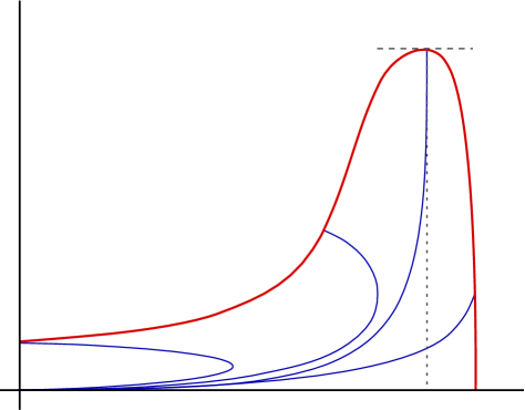
Figure 6.1. A first quadrant view of a control ball centered at the origin.

Definition 34.

Let $\lambda\in(0,\infty)$. The geodesic with turning parameter $\lambda$ first moves to the right and then curls back at the turning point $T\left(\lambda\right)=\left(X\left(\lambda\right),Y\left(\lambda\right)\right)$ when $x=X\left(\lambda\right)\equiv f^{-1}\left(\lambda\right)$. If $R\left(\lambda\right)$ denotes the $A$-arc length from the origin to the turning point $T\left(\lambda\right)$, we have

$$R\left(\lambda\right) \equiv d\left(0,T\left(\lambda\right)\right)=\int_{0}^{X\left(\lambda\right)}\frac{\lambda}{\sqrt{\lambda^{2}-f\left(u\right)^{2}}}du,$$

$$Y\left(\lambda\right) = \int_{0}^{X\left(\lambda\right)}\frac{f\left(u\right)^{2}}{\sqrt{\lambda^{2}-f\left(u\right)^{2}}}du.$$

The two parts of the geodesic $\gamma_{0,\lambda}$,cut at the point $T\left(\lambda\right)$, have different equations:

(6.2) $$y=\left\{\begin{array}[]{ll}\int_{0}^{x}\frac{f\left(u\right)^{2}}{\sqrt{\lambda^{2}-f\left(u\right)^{2}}}du&\text{when}\;y\in\left[0,Y\left(\lambda\right)\right]\\ 2Y\left(\lambda\right)-\int_{0}^{x}\frac{f\left(u\right)^{2}}{\sqrt{\lambda^{2}-f\left(u\right)^{2}}}du&\text{when}\;y\in\left[Y\left(\lambda\right),2Y\left(\lambda\right)\right]\end{array}\right..$$

We define the region covered by the first equation for the geodesics to be Region 1, and the region covered by the second equation for the geodesics to be Region 2. They are separated by the curve $y=Y(f(x))$. We now calculate the first derivative matrix $\begin{bmatrix}\frac{\partial x}{\partial r}&\frac{\partial x}{\partial\lambda}\\ \frac{\partial y}{\partial r}&\frac{\partial y}{\partial\lambda}\end{bmatrix}$ and the Jacobian $\frac{\partial\left(x,y\right)}{\partial\left(r,\lambda\right)}$ in Regions 1 and 2 separately.

6.3.1. Region 1

Applying implicit differentiation to the first equation in (6.1), we have

$$1=\frac{\partial r}{\partial r} =\frac{\partial x}{\partial r}\cdot\frac{\lambda}{\sqrt{\lambda^{2}-f\left(x\right)^{2}}},$$

$$0=\frac{\partial r}{\partial\lambda} =\frac{\partial x}{\partial\lambda}\cdot\frac{\lambda}{\sqrt{\lambda^{2}-f\left(x\right)^{2}}}+\int_{0}^{x}\frac{\partial}{\partial\lambda}\left[\frac{\lambda}{\sqrt{\lambda^{2}-f\left(u\right)^{2}}}\right]du,$$

where

$$\frac{\partial}{\partial\lambda}\left[\frac{\lambda}{\sqrt{\lambda^{2}-f\left(u\right)^{2}}}\right]=\frac{1\cdot\sqrt{\lambda^{2}-f\left(u\right)^{2}}-\lambda\cdot\frac{2\lambda}{2\sqrt{\lambda^{2}-f\left(u\right)^{2}}}}{\lambda^{2}-f\left(u\right)^{2}}=\frac{-f\left(u\right)^{2}}{\left(\lambda^{2}-f\left(u\right)^{2}\right)^{\frac{3}{2}}}.$$

Thus we have

$$\frac{\partial x}{\partial r} = \frac{\sqrt{\lambda^{2}-f\left(x\right)^{2}}}{\lambda},$$

$$\frac{\partial x}{\partial\lambda} = \frac{\sqrt{\lambda^{2}-f\left(x\right)^{2}}}{\lambda}\cdot\int_{0}^{x}\frac{f\left(u\right)^{2}}{\left(\lambda^{2}-f\left(u\right)^{2}\right)^{\frac{3}{2}}}du.$$

Applying implicit differentiation to the second equation in (6.1), we have

$$\frac{\partial y}{\partial r} =\frac{\partial x}{\partial r}\cdot\frac{f\left(x\right)^{2}}{\sqrt{\lambda^{2}-f\left(x\right)^{2}}};$$

$$\frac{\partial y}{\partial\lambda} =\frac{\partial x}{\partial\lambda}\cdot\frac{f\left(x\right)^{2}}{\sqrt{\lambda^{2}-f\left(x\right)^{2}}}+\int_{0}^{x}\frac{\partial}{\partial\lambda}\left[\frac{f\left(u\right)^{2}}{\sqrt{\lambda^{2}-f\left(u\right)^{2}}}\right]du$$

$$=\frac{\partial x}{\partial\lambda}\cdot\frac{f\left(x\right)^{2}}{\sqrt{\lambda^{2}-f\left(x\right)^{2}}}+\int_{0}^{x}\frac{-\lambda f\left(u\right)^{2}}{\left(\lambda^{2}-f\left(u\right)^{2}\right)^{\frac{3}{2}}}du$$

Plugging the equation for $\frac{\partial x}{\partial\lambda}$ into these equations, we obtain

$$\frac{\partial y}{\partial r} = \frac{f\left(x\right)^{2}}{\lambda},$$

$$\frac{\partial y}{\partial\lambda} = \frac{f\left(x\right)^{2}-\lambda^{2}}{\lambda}\cdot\int_{0}^{x}\frac{f\left(u\right)^{2}}{\left(\lambda^{2}-f\left(u\right)^{2}\right)^{\frac{3}{2}}}du,$$

and this completes the calculation of the first derivative matrix $\begin{bmatrix}\frac{\partial x}{\partial r}&\frac{\partial x}{\partial\lambda}\\ \frac{\partial y}{\partial r}&\frac{\partial y}{\partial\lambda}\end{bmatrix}$.

Now we can calculate the Jacobian

$$\frac{\partial\left(x,y\right)}{\partial\left(r,\lambda\right)} = \det\begin{bmatrix}\frac{\sqrt{\lambda^{2}-f\left(x\right)^{2}}}{\lambda}&\frac{\sqrt{\lambda^{2}-f\left(x\right)^{2}}}{\lambda}\cdot\int_{0}^{x}\frac{f\left(u\right)^{2}}{\left(\lambda^{2}-f\left(u\right)^{2}\right)^{\frac{3}{2}}}du\\ \frac{f\left(x\right)^{2}}{\lambda}&\frac{f\left(x\right)^{2}-\lambda^{2}}{\lambda}\cdot\int_{0}^{x}\frac{f\left(u\right)^{2}}{\left(\lambda^{2}-f\left(u\right)^{2}\right)^{\frac{3}{2}}}du\end{bmatrix}$$

$$= -\sqrt{\lambda^{2}-f\left(x\right)^{2}}\int_{0}^{x}\frac{f\left(u\right)^{2}}{\left(\lambda^{2}-f\left(u\right)^{2}\right)^{\frac{3}{2}}}du.$$

In addition we have

$$\int_{0}^{x}\frac{f\left(u\right)^{2}}{\left(\lambda^{2}-f\left(u\right)^{2}\right)^{\frac{3}{2}}}du\approx\int_{x/2}^{x}\frac{f\left(u\right)^{2}}{\left(\lambda^{2}-f\left(u\right)^{2}\right)^{\frac{3}{2}}}du=\int_{x/2}^{x}\frac{\frac{d}{du}\left[f\left(u\right)^{2}\right]\cdot\frac{f\left(u\right)}{2f^{\prime}\left(u\right)}}{\left(\lambda^{2}-f\left(u\right)^{2}\right)^{\frac{3}{2}}}du,$$

where

$$\frac{f\left(u\right)}{2f^{\prime}\left(u\right)}=\frac{1}{-2F^{\prime}\left(u\right)}\approx\frac{1}{-F^{\prime}\left(x\right)},$$

and so we have

$$\int_{0}^{x}\frac{f\left(u\right)^{2}}{\left(\lambda^{2}-f\left(u\right)^{2}\right)^{\frac{3}{2}}}du\approx\frac{1}{-F^{\prime}\left(x\right)}\int_{f\left(\frac{x}{2}\right)^{2}}^{f\left(x\right)^{2}}\frac{1}{\left(\lambda^{2}-v\right)^{\frac{3}{2}}}dv.$$

By Part (1) of Lemma 29, we have $f\left(\frac{x}{2}\right)<\left(\frac{1}{2}\right)^{\varepsilon}f\left(x\right)$, and as a result, we obtain

$$\int_{0}^{x}\frac{f\left(u\right)^{2}}{\left(\lambda^{2}-f\left(u\right)^{2}\right)^{\frac{3}{2}}}du \approx\frac{1}{-F^{\prime}\left(x\right)}\int_{0}^{f\left(x\right)^{2}}\frac{1}{\left(\lambda^{2}-v\right)^{\frac{3}{2}}}dv$$

$$\approx\frac{1}{-F^{\prime}\left(x\right)}\left(\frac{1}{\sqrt{\lambda^{2}-f\left(x\right)^{2}}}-\frac{1}{\lambda}\right).$$

Altogether we have the estimate

(6.3) $$\left|\frac{\partial\left(x,y\right)}{\partial\left(r,\lambda\right)}\right|\approx\frac{1}{-F^{\prime}\left(x\right)}\cdot\frac{\lambda-\sqrt{\lambda^{2}-f\left(x\right)^{2}}}{\lambda}\approx\frac{f\left(x\right)^{2}}{\lambda^{2}\left|F^{\prime}\left(x\right)\right|}.$$

From Corollary 33, we also have

(6.4) $$\left|\frac{\partial\left(x,y\right)}{\partial\left(r,\lambda\right)}\right|\approx\frac{f\left(r\right)^{2}}{\lambda^{2}\left|F^{\prime}\left(r\right)\right|}.$$

6.3.2. Region 2

In Region 2 we have the following pair of formulas:

(6.5) $$r = 2R\left(\lambda\right)-\int_{0}^{x}\frac{\lambda}{\sqrt{\lambda^{2}-f\left(u\right)^{2}}}du\ ,$$

$$y = 2Y\left(\lambda\right)-\int_{0}^{x}\frac{f\left(u\right)^{2}}{\sqrt{\lambda^{2}-f\left(u\right)^{2}}}du\ .$$

where we recall that $R\left(\lambda\right)=\int_{0}^{X\left(\lambda\right)}\frac{\lambda}{\sqrt{\lambda^{2}-f\left(u\right)^{2}}}du$ is the arc length of the geodesic $\gamma_{0,\lambda}$ from the origin $0$ to the turning point $T\left(\lambda\right)$. Before proceeding, we calculate the derivative of $Y\left(\lambda\right)$. We note that due to cancellation, the derivative $R^{\prime}\left(\lambda\right)$ does not explicitly enter into the formula for the Jacobian $\frac{\partial\left(x,y\right)}{\partial\left(r,\lambda\right)}$ below, so we defer its calculation for now.

Lemma 35.

The derivative of $Y\left(\lambda\right)$ is given by

$$Y^{\prime}\left(\lambda\right)=\int_{0}^{f^{-1}\left(\lambda\right)}\frac{F^{\prime\prime}\left(u\right)}{\left|F^{\prime}\left(u\right)\right|^{2}}\frac{\lambda}{\sqrt{\lambda^{2}-f\left(u\right)^{2}}}du.$$

Proof.

Integrating by parts we obtain

$$Y\left(\lambda\right) = \int_{0}^{f^{-1}\left(\lambda\right)}\frac{-f\left(u\right)}{f^{\prime}\left(u\right)}\cdot\frac{d}{du}\sqrt{\lambda^{2}-f\left(u\right)^{2}}du$$

$$= \int_{0}^{f^{-1}\left(\lambda\right)}\frac{1}{F^{\prime}\left(u\right)}\cdot\frac{d}{du}\sqrt{\lambda^{2}-f\left(u\right)^{2}}du$$

$$= -\int_{0}^{f^{-1}\left(\lambda\right)}\sqrt{\lambda^{2}-f\left(u\right)^{2}}\cdot\frac{d}{du}\frac{1}{F^{\prime}\left(u\right)}du$$

$$= \int_{0}^{f^{-1}\left(\lambda\right)}\frac{F^{\prime\prime}\left(u\right)}{\left|F^{\prime}\left(u\right)\right|^{2}}\sqrt{\lambda^{2}-f\left(u\right)^{2}}du,$$

and so from $\lambda^{2}-f\left(f^{-1}\left(\lambda\right)\right)^{2}=0$, we have

$$Y^{\prime}\left(\lambda\right)=0+\int_{0}^{f^{-1}\left(\lambda\right)}\frac{F^{\prime\prime}\left(u\right)}{\left|F^{\prime}\left(u\right)\right|^{2}}\frac{\lambda}{\sqrt{\lambda^{2}-f\left(u\right)^{2}}}du.$$

   

Applying implicit differentiation to the first equation in (6.5), we have

$$1=\frac{\partial r}{\partial r} =-\frac{\partial x}{\partial r}\cdot\frac{\lambda}{\sqrt{\lambda^{2}-f\left(x\right)^{2}}},$$

$$0=\frac{\partial r}{\partial\lambda} =2R^{\prime}\left(\lambda\right)-\frac{\partial x}{\partial\lambda}\cdot\frac{\lambda}{\sqrt{\lambda^{2}-f\left(x\right)^{2}}}-\int_{0}^{x}\frac{\partial}{\partial\lambda}\left[\frac{\lambda}{\sqrt{\lambda^{2}-f\left(u\right)^{2}}}\right]du,$$

where

$$\frac{\partial}{\partial\lambda}\left[\frac{\lambda}{\sqrt{\lambda^{2}-f\left(u\right)^{2}}}\right]=\frac{1\cdot\sqrt{\lambda^{2}-f\left(u\right)^{2}}-\lambda\cdot\frac{2\lambda}{2\sqrt{\lambda^{2}-f\left(u\right)^{2}}}}{\lambda^{2}-f\left(u\right)^{2}}=\frac{-f\left(u\right)^{2}}{\left(\lambda^{2}-f\left(u\right)^{2}\right)^{\frac{3}{2}}}.$$

Thus we have

$$\frac{\partial x}{\partial r} = -\frac{\sqrt{\lambda^{2}-f\left(x\right)^{2}}}{\lambda},$$

$$\frac{\partial x}{\partial\lambda} = \frac{2\sqrt{\lambda^{2}-f\left(x\right)^{2}}}{\lambda}L^{\prime}\left(\lambda\right)+\frac{\sqrt{\lambda^{2}-f\left(x\right)^{2}}}{\lambda}\cdot\int_{0}^{x}\frac{f\left(u\right)^{2}}{\left(\lambda^{2}-f\left(u\right)^{2}\right)^{\frac{3}{2}}}du.$$

Applying implicit differentiation to the second equation in (6.5), we have

$$\frac{\partial y}{\partial r} =-\frac{\partial x}{\partial r}\cdot\frac{f\left(x\right)^{2}}{\sqrt{\lambda^{2}-f\left(x\right)^{2}}};$$

$$\frac{\partial y}{\partial\lambda} =2Y^{\prime}\left(\lambda\right)-\frac{\partial x}{\partial\lambda}\cdot\frac{f\left(x\right)^{2}}{\sqrt{\lambda^{2}-f\left(x\right)^{2}}}-\int_{0}^{x}\frac{\partial}{\partial\lambda}\left[\frac{f\left(u\right)^{2}}{\sqrt{\lambda^{2}-f\left(u\right)^{2}}}\right]du$$

$$=2Y^{\prime}\left(\lambda\right)-\frac{\partial x}{\partial\lambda}\cdot\frac{f\left(x\right)^{2}}{\sqrt{\lambda^{2}-f\left(x\right)^{2}}}-\int_{0}^{x}\frac{-\lambda f\left(u\right)^{2}}{\left(\lambda^{2}-f\left(u\right)^{2}\right)^{\frac{3}{2}}}du$$

Plugging the equation for $\frac{\partial x}{\partial\lambda}$ above into these equations, we have

$$\frac{\partial y}{\partial r} = \frac{f\left(x\right)^{2}}{\lambda},$$

$$\frac{\partial y}{\partial\lambda} = 2Y^{\prime}\left(\lambda\right)-\frac{2f\left(x\right)^{2}}{\lambda}R^{\prime}\left(\lambda\right)+\frac{\lambda^{2}-f\left(x\right)^{2}}{\lambda}\cdot\int_{0}^{x}\frac{f\left(u\right)^{2}}{\left(\lambda^{2}-f\left(u\right)^{2}\right)^{\frac{3}{2}}}du.$$

Thus the Jacobian is given by

$$\frac{\partial\left(x,y\right)}{\partial\left(r,\lambda\right)}$$

$$=\det\begin{bmatrix}-\frac{\sqrt{\lambda^{2}-f\left(x\right)^{2}}}{\lambda}&\frac{2\sqrt{\lambda^{2}-f\left(x\right)^{2}}}{\lambda}R^{\prime}\left(\lambda\right)+\frac{\sqrt{\lambda^{2}-f\left(x\right)^{2}}}{\lambda}\cdot\int_{0}^{x}\frac{f\left(u\right)^{2}}{\left(\lambda^{2}-f\left(u\right)^{2}\right)^{\frac{3}{2}}}du\\ \frac{f\left(x\right)^{2}}{\lambda}&2Y^{\prime}\left(\lambda\right)-\frac{2f\left(x\right)^{2}}{\lambda}R^{\prime}\left(\lambda\right)+\frac{\lambda^{2}-f\left(x\right)^{2}}{\lambda}\cdot\int_{0}^{x}\frac{f\left(u\right)^{2}}{\left(\lambda^{2}-f\left(u\right)^{2}\right)^{\frac{3}{2}}}du\end{bmatrix}$$

$$=\det\begin{bmatrix}-\frac{\sqrt{\lambda^{2}-f\left(x\right)^{2}}}{\lambda}&\frac{\sqrt{\lambda^{2}-f\left(x\right)^{2}}}{\lambda}\cdot\int_{0}^{x}\frac{f\left(u\right)^{2}}{\left(\lambda^{2}-f\left(u\right)^{2}\right)^{\frac{3}{2}}}du\\ \frac{f\left(x\right)^{2}}{\lambda}&2Y^{\prime}\left(\lambda\right)+\frac{\lambda^{2}-f\left(x\right)^{2}}{\lambda}\cdot\int_{0}^{x}\frac{f\left(u\right)^{2}}{\left(\lambda^{2}-f\left(u\right)^{2}\right)^{\frac{3}{2}}}du\end{bmatrix}$$

$$=-\sqrt{\lambda^{2}-f\left(x\right)^{2}}\left\{\int_{0}^{x}\frac{f\left(u\right)^{2}}{\left(\lambda^{2}-f\left(u\right)^{2}\right)^{\frac{3}{2}}}du+\frac{2}{\lambda}Y^{\prime}\left(\lambda\right)\right\}$$

$$=-\sqrt{\lambda^{2}-f\left(x\right)^{2}}\left\{\int_{0}^{x}\frac{f\left(u\right)^{2}}{\left(\lambda^{2}-f\left(u\right)^{2}\right)^{\frac{3}{2}}}du+\frac{2}{\lambda}\int\limits_{0}^{f^{-1}\left(\lambda\right)}\frac{F^{\prime\prime}\left(u\right)}{\left|F^{\prime}\left(u\right)\right|^{2}}\frac{\lambda}{\sqrt{\lambda^{2}-f\left(u\right)^{2}}}du\right\}$$

$$=-\sqrt{\lambda^{2}-f\left(x\right)^{2}}\left\{\int_{0}^{x}\frac{f\left(u\right)^{2}}{\left(\lambda^{2}-f\left(u\right)^{2}\right)^{\frac{3}{2}}}du+\int\limits_{0}^{f^{-1}(\lambda)}\frac{F^{\prime\prime}\left(u\right)}{\left|F^{\prime}\left(u\right)\right|^{2}}\cdot\frac{2}{\sqrt{\lambda^{2}-f\left(u\right)^{2}}}du\right\}.$$

In fact, we have

$$\int_{0}^{x} \frac{f\left(u\right)^{2}}{\left(\lambda^{2}-f\left(u\right)^{2}\right)^{\frac{3}{2}}}du=\int_{0}^{x}\frac{f\left(u\right)}{f^{\prime}\left(u\right)}\cdot\frac{d}{du}\left[\frac{1}{\sqrt{\lambda^{2}-f\left(u\right)^{2}}}\right]du$$

$$=\int_{0}^{x}\frac{1}{-F^{\prime}\left(u\right)}\cdot\frac{d}{du}\left[\frac{1}{\sqrt{\lambda^{2}-f\left(u\right)^{2}}}\right]du$$

$$=\frac{1}{-F^{\prime}\left(x\right)}\cdot\frac{1}{\sqrt{\lambda^{2}-f\left(x\right)^{2}}}-\int_{0}^{x}\frac{1}{\sqrt{\lambda^{2}-f\left(u\right)^{2}}}\cdot\frac{d}{du}\left[\frac{1}{-F^{\prime}\left(u\right)}\right]du$$

$$=\frac{1}{-F^{\prime}\left(x\right)}\cdot\frac{1}{\sqrt{\lambda^{2}-f\left(x\right)^{2}}}-\int_{0}^{x}\frac{1}{\sqrt{\lambda^{2}-f\left(u\right)^{2}}}\cdot\frac{F^{\prime\prime}\left(u\right)}{\left|F^{\prime}\left(u\right)\right|^{2}}du$$

As a result, we have within a factor of $2$,

(6.6) $$\left|\frac{\partial\left(x,y\right)}{\partial\left(r,\lambda\right)}\right|\approx \sqrt{\lambda^{2}-f\left(x\right)^{2}}\left\{\frac{1}{-F^{\prime}\left(x\right)}\cdot\frac{1}{\sqrt{\lambda^{2}-f\left(x\right)^{2}}}\right.$$

$$\qquad\qquad\qquad\qquad+\left.\int_{0}^{f^{-1}\left(\lambda\right)}\frac{F^{\prime\prime}\left(u\right)}{\left|F^{\prime}\left(u\right)\right|^{2}}\cdot\frac{1}{\sqrt{\lambda^{2}-f\left(u\right)^{2}}}du\right\}$$

$$= \frac{1}{-F^{\prime}\left(x\right)}+\sqrt{\lambda^{2}-f\left(x\right)^{2}}\int_{0}^{f^{-1}\left(\lambda\right)}\frac{F^{\prime\prime}\left(u\right)}{\left|F^{\prime}\left(u\right)\right|^{2}}\cdot\frac{1}{\sqrt{\lambda^{2}-f\left(u\right)^{2}}}du.$$

By Assumption (5), we have

$$\int_{0}^{f^{-1}\left(\lambda\right)}\frac{F^{\prime\prime}\left(u\right)}{\left|F^{\prime}\left(u\right)\right|^{2}}\cdot\frac{1}{\sqrt{\lambda^{2}-f\left(u\right)^{2}}}du\approx\int_{0}^{f^{-1}\left(\lambda\right)}\frac{1}{-uF^{\prime}\left(u\right)}\cdot\frac{1}{\sqrt{\lambda^{2}-f\left(u\right)^{2}}}du.$$

By Assumptions (3) and (4), the function $\frac{1}{-uF^{\prime}\left(u\right)}$ increases and satisfies the doubling property, and so

(6.7) $$\int_{0}^{f^{-1}\left(\lambda\right)}\frac{F^{\prime\prime}\left(u\right)}{\left|F^{\prime}\left(u\right)\right|^{2}} \cdot\frac{1}{\sqrt{\lambda^{2}-f\left(u\right)^{2}}}du$$

$$\approx\frac{1}{-f^{-1}\left(\lambda\right)F^{\prime}\left(f^{-1}\left(\lambda\right)\right)}\int_{0}^{f^{-1}\left(\lambda\right)}\frac{1}{\sqrt{\lambda^{2}-f\left(u\right)^{2}}}du$$

$$=\frac{1}{-f^{-1}\left(\lambda\right)F^{\prime}\left(f^{-1}\left(\lambda\right)\right)}\frac{R\left(\lambda\right)}{\lambda}$$

$$\simeq\frac{1}{-\lambda F^{\prime}\left(f^{-1}\left(\lambda\right)\right)}$$

since $R\left(\lambda\right)\approx f^{-1}\left(\lambda\right)$ by Lemma 32. Finally we can combine (6.6) and (6.7) to obtain

$$\left|\frac{\partial\left(x,y\right)}{\partial\left(r,\lambda\right)}\right|\approx\frac{1}{-F^{\prime}\left(x\right)}+\frac{\sqrt{\lambda^{2}-f\left(x\right)^{2}}}{\lambda}\cdot\frac{1}{-F^{\prime}\left(f^{-1}\left(\lambda\right)\right)}\approx\frac{1}{-F^{\prime}\left(f^{-1}\left(\lambda\right)\right)}.$$

According to Corollary 33, we also have

$$\left|\frac{\partial\left(x,y\right)}{\partial\left(r,\lambda\right)}\right|\approx\frac{1}{-F^{\prime}(R\left(\lambda\right))}.$$

6.3.3. Integral of Radial Functions

Summarizing our estimates on the Jacobian we have

$$\left|\frac{\partial\left(x,y\right)}{\partial\left(r,\lambda\right)}\right|\approx\left\{\begin{array}[]{ll}\frac{f\left(r\right)^{2}}{\lambda^{2}\left|F^{\prime}\left(r\right)\right|}\simeq\frac{f\left(x\right)^{2}}{\lambda^{2}\left|F^{\prime}\left(x\right)\right|}&\text{when}\;r<R\left(\lambda\right)\\ &\\ \frac{1}{\left|F^{\prime}\left(f^{-1}\left(\lambda\right)\right)\right|}\simeq\frac{1}{\left|F^{\prime}\left(R\left(\lambda\right)\right)\right|}&\text{when}\;R\left(\lambda\right)<r<2R\left(\lambda\right)\end{array}\right..$$

Therefore we have the following change of variable formula for nonnegative functions $w$:

$$\iint_{QB\left(0,r_{0}\right)}wdxdy=\int_{0}^{r_{0}}\left[\int_{R^{-1}\left(\frac{r}{2}\right)}^{\infty}w\left|\frac{\partial(x,y)}{\partial(r,\lambda)}\right|d\lambda\right]dr$$

$$\approx\int_{0}^{r_{0}}\left[\int_{R^{-1}\left(\frac{r}{2}\right)}^{R^{-1}\left(r\right)}w\left(r,\lambda\right)\frac{1}{\left|F^{\prime}\left(R\left(\lambda\right)\right)\right|}d\lambda+\int_{R^{-1}\left(r\right)}^{\infty}w\left(r,\lambda\right)\frac{f\left(r\right)^{2}}{\lambda^{2}\left|F^{\prime}\left(r\right)\right|}d\lambda\right]dr$$

$$\approx\int_{0}^{r_{0}}\left[\int_{R^{-1}\left(\frac{r}{2}\right)}^{R^{-1}\left(r\right)}w(r,\lambda)\frac{1}{|F^{\prime}(r)|}d\lambda+\int_{R^{-1}(r)}^{\infty}w(r,\lambda)\frac{f^{2}(r)}{\lambda^{2}|F^{\prime}(r)|}d\lambda\right]dr$$

If $w$ is a radial function, then we have

$$\iint_{QB\left(0,r_{0}\right)}wdxdy \approx\int_{0}^{r_{0}}w\left(r\right)\left[\int_{R^{-1}\left(\frac{r}{2}\right)}^{R^{-1}\left(r\right)}\frac{1}{\left|F^{\prime}\left(r\right)\right|}d\lambda+\int_{R^{-1}\left(r\right)}^{\infty}\frac{f\left(r\right)^{2}}{\lambda^{2}\left|F^{\prime}\left(r\right)\right|}d\lambda\right]dr$$

$$\approx\int_{0}^{r_{0}}w\left(r\right)\left[\frac{R^{-1}\left(r\right)-R^{-1}\left(\frac{r}{2}\right)}{\left|F^{\prime}\left(r\right)\right|}+\frac{f\left(r\right)^{2}}{R^{-1}\left(r\right)\left|F^{\prime}\left(r\right)\right|}\right]dr.$$

From Corollary 33, we have $R^{-1}\left(r\right)\simeq f\left(r\right)$, and so we have

(6.8) $$\iint_{B\left(0,r_{0}\right)}w\left(r\right)dxdy\approx\int_{0}^{r_{0}}w\left(r\right)\frac{f\left(r\right)}{\left|F^{\prime}\left(r\right)\right|}dr.$$

Conclusion 36.

The area of the $A$-ball $B\left(0,r_{0}\right)$ satisfies

(6.9) $$\left|B\left(0,r_{0}\right)\right|=\iint_{B\left(0,r_{0}\right)}dxdy\approx\int_{0}^{r_{0}}\frac{f\left(r\right)}{\left|F^{\prime}\left(r\right)\right|}dr\approx\frac{f\left(r_{0}\right)}{\left|F^{\prime}\left(r_{0}\right)\right|^{2}}.$$

Proof.

Since $F\left(r\right)=-\ln f\left(r\right)$, we have $F^{\prime}\left(r\right)=-\frac{f^{\prime}\left(r\right)}{f\left(r\right)}$ and $\frac{f\left(r\right)}{-F^{\prime}\left(r\right)}=\frac{f\left(r\right)^{2}}{f^{\prime}\left(r\right)}=\frac{f\left(r\right)^{2}}{f^{\prime}\left(r\right)^{2}}f^{\prime}\left(r\right)=\frac{f^{\prime}\left(r\right)}{\left|F^{\prime}\left(r\right)\right|^{2}}$, and so

$$\iint_{B\left(0,r_{0}\right)}dxdy \approx \int_{0}^{r_{0}}\frac{f\left(r\right)}{\left|F^{\prime}\left(r\right)\right|}dr\approx\int_{\frac{r_{0}}{2}}^{r_{0}}\frac{f\left(r\right)}{\left|F^{\prime}\left(r\right)\right|}dr=\int_{\frac{r_{0}}{2}}^{r_{0}}\frac{f^{\prime}\left(r\right)}{\left|F^{\prime}\left(r\right)\right|^{2}}dr$$

$$\approx \frac{1}{\left|F^{\prime}\left(r_{0}\right)\right|^{2}}\int_{\frac{r_{0}}{2}}^{r_{0}}f^{\prime}\left(r\right)dr=\frac{f\left(r_{0}\right)-f\left(\frac{r_{0}}{2}\right)}{\left|F^{\prime}\left(r_{0}\right)\right|^{2}}\approx\frac{f\left(r_{0}\right)}{\left|F^{\prime}\left(r_{0}\right)\right|^{2}}.$$

   

6.3.4. Balls centered at an arbitrary point

In this section we consider the “height” of an arbitrary $A$-ball and the relative position at which it is achieved in the ball.

Definition 37.

Let $X=(x_{1},0)$ be a point on the positive $x$-axis and let $r$ be a positive real number. Let the upper half of the boundary of the ball $B\left(X,r\right)$ be given as a graph of the function $\varphi\left(x\right)$, $x_{1}-r<x<x_{1}+r$. Denote by $\beta_{X,Q}$ the geodesic connecting the center $X$ of the ball $B\left(X,r\right)$ with a point $Q$ on the boundary $\partial B\left(X,r\right)$ of the ball $B\left(X,r\right)$.
Denote by $P=P_{x_{1},r}=\left(x_{1}+r^{\ast},h\right)$ the unique point on the boundary $\partial B\left(X,r\right)$ of the ball $B\left(X,r\right)$ with $r^{\ast}>0$ and $h>0$ at which the geodesic $\beta_{X,P}$ connecting $X$ and $P$ has a vertical tangent at $P$. This defines

$$r^{\ast}=r^{\ast}\left(x_{1},r\right)\text{ and }h=h\left(x_{1},r\right)=\varphi\left(x_{1}+r^{\ast}\right)$$

implicitly as functions of the two independent variables $x_{1}$ and $r$.

We will often write simply $r^{\ast}$ and $h$ in place of $r^{\ast}\left(x_{1},r\right)$ and $h\left(x_{1},r\right)$ respectively when $x_{1}$ and $r$ are understood. See figure 6.2.

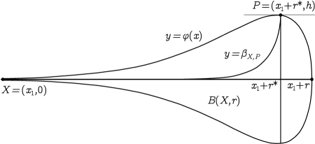
Figure 6.2. The right ‘half’ of a control ball centered at $\left(x_{1},0\right)$.

Proposition 38.

Let $\beta_{X,P}$, $r^{\ast}$ and $h$ be defined as above. Define $\lambda\left(x\right)$ implicitly by

$$r=\int_{x_{1}}^{x}\frac{\lambda\left(x\right)}{\sqrt{\lambda\left(x\right)^{2}-f\left(u\right)^{2}}}du.$$

Then

1. For $x_{1}-r<x<x_{1}+r$ we have $\varphi\left(x\right)\leq\varphi\left(x_{1}+r^{\ast}\right)=h$.

2. If $r\geq\frac{1}{\left|F^{\prime}\left(x_{1}\right)\right|}$, then

   $$h\approx\frac{f\left(x_{1}+r\right)}{\left|F^{\prime}\left(x_{1}+r\right)\right|}\text{ and }r-r^{\ast}\approx\frac{1}{\left|F^{\prime}\left(x_{1}+r\right)\right|}.$$

3. If $r\leq\frac{1}{\left|F^{\prime}\left(x_{1}\right)\right|}$, then

   $$h\approx rf\left(x_{1}\right)\text{ and }r-r^{\ast}\approx r.$$

We begin by proving part (1) of Proposition 38. First consider the case $x\geq x_{1}+r^{\ast}$. Then we are in Region 1 and so $\lambda\left(x\right)\geq f\left(x\right)$ and we have

$$\varphi\left(x\right)=\int_{x_{1}}^{x}\frac{f\left(u\right)^{2}}{\sqrt{\lambda\left(x\right)^{2}-f\left(u\right)^{2}}}du.$$

Differentiating $\varphi\left(x\right)$ we get

$$\varphi^{\prime}\left(x\right)=\frac{f\left(x\right)^{2}}{\sqrt{\lambda\left(x\right)^{2}-f\left(x\right)^{2}}}-\left(\int_{x_{1}}^{x}\frac{f\left(u\right)^{2}}{\left(\lambda\left(x\right)^{2}-f\left(u\right)^{2}\right)^{\frac{3}{2}}}du\right)\lambda\left(x\right)\lambda^{\prime}\left(x\right),$$

and differentiating the definition of $\lambda\left(x\right)$ implicitly gives

$$0=\frac{\lambda\left(x\right)}{\sqrt{\lambda\left(x\right)^{2}-f\left(x\right)^{2}}}-\left(\int_{x_{1}}^{x}\frac{f\left(u\right)^{2}}{\left(\lambda\left(x\right)^{2}-f\left(u\right)^{2}\right)^{\frac{3}{2}}}du\right)\lambda^{\prime}\left(x\right).$$

Combining equalities yields

$$\varphi^{\prime}\left(x\right)=\frac{f\left(x\right)^{2}}{\sqrt{\lambda\left(x\right)^{2}-f\left(x\right)^{2}}}-\lambda\left(x\right)\frac{\lambda\left(x\right)}{\sqrt{\lambda\left(x\right)^{2}-f\left(x\right)^{2}}}=-\sqrt{\lambda\left(x\right)^{2}-f\left(x\right)^{2}}.$$

When $x=x_{1}+r^{\ast}$ we have $\infty=\frac{dy}{dx}=\frac{f\left(x\right)^{2}}{\sqrt{\lambda\left(x\right)^{2}-f\left(x\right)^{2}}}$, which implies $\lambda\left(x\right)=f\left(x\right)$, and hence $\varphi^{\prime}\left(x_{1}+r^{\ast}\right)=0$. Thus we have $\varphi\left(x\right)\leq\varphi\left(x_{1}+r^{\ast}\right)=h$ for $x\geq x_{1}+r^{\ast}$. Similar arguments show that $\varphi\left(x\right)\leq\varphi\left(x_{1}+r^{\ast}\right)=h$ for $x_{1}-r\leq x<x_{1}+r^{\ast}$, and this completes the proof of part (1).

Now we turn to the proofs of parts (2) and (3) of Proposition 38. The locus $\left(x,y\right)$ of the geodesic $\beta_{X,P}$ satisfies

(6.10) $$y=\int_{x_{1}}^{x}\frac{f\left(u\right)^{2}}{\sqrt{\left(\lambda^{\ast}\right)^{2}-f\left(u\right)^{2}}}\,du,$$

where $\lambda^{\ast}=f\left(x_{1}+r^{\ast}\right)$. We will use the following two lemmas in the proofs of parts (2) and (3) of Proposition 38.

Lemma 39.

The height $h=h\left(x_{1},r\right)$ and the horizontal displacement $r-r^{\ast}=r-r^{\ast}\left(x_{1},r\right)$ satisfy

$$f\left(x_{1}+r^{\ast}\right)\cdot\left(r-r^{\ast}\right)\leq h\leq 2f\left(x_{1}+r^{\ast}\right)\cdot\left(r-r^{\ast}\right).$$

Proof.

The $A$-arc length $r$ of $\beta_{X,P}$ is given by

$$r=\int_{x_{1}}^{x_{1}+r^{\ast}}\frac{\lambda^{\ast}}{\sqrt{\left(\lambda^{\ast}\right)^{2}-f\left(u\right)^{2}}}\,du.$$

Thus

$$r-r^{\ast} =\int_{x_{1}}^{x_{1}+r^{\ast}}\left(\frac{\lambda^{\ast}}{\sqrt{\left(\lambda^{\ast}\right)^{2}-f\left(u\right)^{2}}}-1\right)\,du$$

$$=\int_{x_{1}}^{x_{1}+r^{\ast}}\frac{f\left(u\right)^{2}}{\sqrt{\left(\lambda^{\ast}\right)^{2}-f\left(u\right)^{2}}}\cdot\frac{1}{\lambda^{\ast}+\sqrt{\left(\lambda^{\ast}\right)^{2}-f\left(u\right)^{2}}}\,du$$

Comparing this with the height $h=\int_{x_{1}}^{x_{1}+r^{\ast}}\frac{f^{2}(u)}{\sqrt{\left(\lambda^{\ast}\right)^{2}-f\left(u\right)^{2}}}\,du$, we have

$$\frac{h}{2\lambda^{\ast}}\leq r-r^{\ast}\leq\frac{h}{\lambda^{\ast}}.$$

This completes the proof since $\lambda^{\ast}=f\left(x_{1}+r^{\ast}\right)$.    

Lemma 40.

The height $h$ satisfies the estimate

$$h\approx\frac{1}{\left|F^{\prime}\left(x_{1}+r^{\ast}\right)\right|}\sqrt{f\left(x_{1}+r^{\ast}\right)^{2}-f\left(x_{1}\right)^{2}}.$$

In fact the right hand side is an exact upper bound:

$$h\leq\frac{1}{\left|F^{\prime}\left(x_{1}+r^{\ast}\right)\right|}\sqrt{f\left(x_{1}+r^{\ast}\right)^{2}-f\left(x_{1}\right)^{2}}.$$

Proof.

Using the fact that $\frac{1}{-F^{\prime}\left(u\right)}=\frac{1}{\left|F^{\prime}\left(u\right)\right|}$ is increasing, together with the equation (6.10) for the geodesic $\beta_{X,P}$, we have

$$h\left(x_{1},r\right)= \int_{x_{1}}^{x_{1}+r^{\ast}\left(x_{1},r\right)}\frac{f\left(u\right)^{2}}{\sqrt{\left(\lambda^{\ast}\right)^{2}-f\left(u\right)^{2}}}\,du$$

$$= \int_{x_{1}}^{x_{1}+r^{\ast}}\frac{\frac{d}{du}\left[f\left(u\right)^{2}\right]}{\sqrt{\left(\lambda^{\ast}\right)^{2}-f\left(u\right)^{2}}}\cdot\frac{1}{-2F^{\prime}\left(u\right)}\,du$$

$$\leq \frac{1}{\left|F^{\prime}\left(x_{1}+r^{\ast}\right)\right|}\int_{x_{1}}^{x_{1}+r^{\ast}}\frac{\frac{d}{du}\left[f\left(u\right)^{2}\right]}{2\sqrt{\left(\lambda^{\ast}\right)^{2}-f\left(u\right)^{2}}}\,du$$

$$= \frac{1}{\left|F^{\prime}\left(x_{1}+r^{\ast}\right)\right|}\sqrt{f\left(x_{1}+r^{\ast}\right)^{2}-f\left(x_{1}\right)^{2}},$$

where in the last line we used $\lambda^{\ast}=f\left(x_{1}+r^{\ast}\right)$. To prove the reverse estimate, we consider two cases:

Case 1: If $r^{\ast}<x_{1}$, then we use our assumption that $\frac{1}{-F^{\prime}\left(u\right)}=\frac{1}{\left|F^{\prime}\left(u\right)\right|}$ has the doubling property to obtain

$$h=\int_{x_{1}}^{x_{1}+r^{\ast}}\frac{f\left(u\right)^{2}}{\sqrt{\left(\lambda^{\ast}\right)^{2}-f\left(u\right)^{2}}}\,du= \int_{x_{1}}^{x_{1}+r^{\ast}}\frac{\frac{d}{du}\left[f\left(u\right)^{2}\right]}{\sqrt{\left(\lambda^{\ast}\right)^{2}-f\left(u\right)^{2}}}\cdot\frac{1}{-2F^{\prime}\left(u\right)}\,du$$

$$\simeq \frac{1}{\left|F^{\prime}\left(x_{1}+r^{\ast}\right)\right|}\int_{x_{1}}^{x_{1}+r^{\ast}}\frac{\frac{d}{du}\left[f\left(u\right)^{2}\right]}{2\sqrt{\left(\lambda^{\ast}\right)^{2}-f\left(u\right)^{2}}}\,du$$

$$= \frac{1}{\left|F^{\prime}\left(x_{1}+r^{\ast}\right)\right|}\sqrt{f\left(x_{1}+r^{\ast}\right)^{2}-f\left(x_{1}\right)^{2}}.$$

Case 2: If $r^{\ast}\geq x_{1}$, we make a similar estimate by modifying the lower limit of integral, and using the fact that $f\left(u\right)$ increases:

$$h\approx\int_{x_{1}+\frac{r^{\ast}}{2}}^{x_{1}+r^{\ast}}\frac{f\left(u\right)^{2}}{\sqrt{\left(\lambda^{\ast}\right)^{2}-f\left(u\right)^{2}}}\,du= \int_{x_{1}+\frac{r^{\ast}}{2}}^{x_{1}+r^{\ast}}\frac{\frac{d}{du}\left[f\left(u\right)^{2}\right]}{\sqrt{\left(\lambda^{\ast}\right)^{2}-f\left(u\right)^{2}}}\cdot\frac{1}{-2F^{\prime}\left(u\right)}\,du$$

$$\approx \frac{1}{\left|F^{\prime}\left(x_{1}+r^{\ast}\right)\right|}\int_{x_{1}+\frac{r^{\ast}}{2}}^{x_{1}+r^{\ast}}\frac{\frac{d}{du}\left[f\left(u\right)^{2}\right]}{2\sqrt{\left(\lambda^{\ast}\right)^{2}-f\left(u\right)^{2}}}\,du$$

$$= \frac{1}{\left|F^{\prime}\left(x_{1}+r^{\ast}\right)\right|}\sqrt{f\left(x_{1}+r^{\ast}\right)^{2}-f\left(x_{1}+\frac{r^{\ast}}{2}\right)^{2}}.$$

Finally we have

$$\sqrt{f\left(x_{1}+r^{\ast}\right)^{2}-f\left(x_{1}+\frac{r^{\ast}}{2}\right)^{2}}\approx f\left(x_{1}+r^{\ast}\right)\approx\sqrt{f\left(x_{1}+r^{\ast}\right)^{2}-f\left(x_{1}\right)^{2}}$$

by the assumption $r^{\ast}\geq x_{1}$ together with Part 1 of Lemma 29.

This completes the proof of Lemma 40.    

Corollary 41.

Combining Lemmas 39 and 40, for $h=h\left(x_{1},r\right)$ and $r^{\ast}=r^{\ast}\left(x_{1},r\right)$, we have

$$f\left(x_{1}+r^{\ast}\right)\cdot\left(r-r^{\ast}\right)\leq h\leq\frac{1}{\left|F^{\prime}\left(x_{1}+r^{\ast}\right)\right|}\sqrt{f\left(x_{1}+r^{\ast}\right)^{2}-f\left(x_{1}\right)^{2}},$$

and as a result,

(6.11) $$r-r^{\ast}\leq\frac{1}{\left|F^{\prime}\left(x_{1}+r^{\ast}\right)\right|}\cdot\frac{\sqrt{f\left(x_{1}+r^{\ast}\right)^{2}-f\left(x_{1}\right)^{2}}}{f\left(x_{1}+r^{\ast}\right)}\leq\frac{1}{\left|F^{\prime}\left(x_{1}+r^{\ast}\right)\right|}.$$

From part (2) of Lemma 29 we obtain

(6.12) $$\left|F^{\prime}\left(x_{1}+r\right)\right| \approx \left|F^{\prime}\left(x_{1}+r^{\ast}\right)\right|,$$

$$f\left(x_{1}+r\right) \simeq f\left(x_{1}+r^{\ast}\right).$$

We now split the proof of Proposition 38 into two cases.

Proof of part (2) of Proposition 38 for $r\geq\frac{1}{\left|F^{\prime}\left(x_{1}\right)\right|}$

By Lemmas 39 and 40, we have

(6.13) $$r-r^{\ast}\left(x_{1},r\right)=r-r^{\ast}\approx\frac{1}{\left|F^{\prime}\left(x_{1}+r^{\ast}\right)\right|}\cdot\frac{\sqrt{f\left(x_{1}+r^{\ast}\right)^{2}-f\left(x_{1}\right)^{2}}}{f\left(x_{1}+r^{\ast}\right)}.$$

We consider two cases.

Case A: If $r^{\ast}>r_{1}\equiv\frac{1}{2\left|F^{\prime}\left(x_{1}\right)\right|}$, then we have

$$F\left(x_{1}\right)-F\left(x_{1}+r^{\ast}\right)=\int_{x_{1}}^{x_{1}+r^{\ast}}\left|F^{\prime}\left(x_{1}\right)\right|dx \geq\int_{x_{1}}^{x_{1}+r_{1}}\left|F^{\prime}\left(x_{1}\right)\right|dx$$

$$\geq\left|F^{\prime}\left(x_{1}+r_{1}\right)\right|\cdot r_{1}\gtrsim 1.$$

Here we used the estimate $\left|F^{\prime}\left(x_{1}+r_{1}\right)\right|\approx\left|F^{\prime}\left(x_{1}\right)\right|$ given by Part 2 of Lemma 29. This implies

$$\ln\frac{f\left(x_{1}+r^{\ast}\right)}{f\left(x_{1}\right)}\gtrsim 1,$$

and we have

$$\frac{\sqrt{f\left(x_{1}+r^{\ast}\right)^{2}-f\left(x_{1}\right)^{2}}}{f\left(x_{1}+r^{\ast}\right)}\approx 1.$$

Plugging this into (6.13), we have $r-r^{\ast}\approx\frac{1}{\left|F^{\prime}\left(x_{1}+r^{\ast}\right)\right|}$. The proof is completed using (6.12) and Lemma 39.

Case B: If $r^{\ast}\leq r_{1}$, then we have $\left|F^{\prime}\left(x_{1}+r^{\ast}\right)\right|\approx\left|F^{\prime}\left(x_{1}\right)\right|$ and $r-r^{\ast}\geq\frac{1}{2\left|F^{\prime}\left(x_{1}\right)\right|}$. Therefore we have

$$r-r^{\ast}\gtrsim\frac{1}{\left|F^{\prime}\left(x_{1}+r^{\ast}\right)\right|}.$$

Combining this with (6.11), we obtain $r-r^{\ast}\approx\frac{1}{\left|F^{\prime}\left(x_{1}+r^{\ast}\right)\right|}$ again, and the proof is completed as in the first case.

Proof of part (3) of Proposition 38 for $r\leq\frac{1}{\left|F^{\prime}\left(x_{1}\right)\right|}$

In this case Lemma 39 and Lemma 40 give with $r^{\ast}=r^{\ast}\left(x_{1},r\right)$,

$$f\left(x_{1}+r^{\ast}\right)\cdot\left(r-r^{\ast}\right)\approx h\left(x_{1},r\right) \approx\frac{1}{\left|F^{\prime}\left(x_{1}+r^{\ast}\right)\right|}\sqrt{f\left(x_{1}+r^{\ast}\right)^{2}-f\left(x_{1}\right)^{2}}$$

$$\approx\frac{1}{\left|F^{\prime}\left(x_{1}\right)\right|}\left(\int_{x_{1}}^{x_{1}+r^{\ast}}2f\left(u\right)^{2}\left|F^{\prime}\left(u\right)\right|\,du\right)^{\frac{1}{2}}$$

$$\approx\frac{1}{\left|F^{\prime}\left(x_{1}\right)\right|}\left[2f\left(x_{1}+r^{\ast}\right)^{2}\left|F^{\prime}\left(x_{1}\right)\right|\cdot r^{\ast}\right]^{\frac{1}{2}}$$

$$\approx\frac{\sqrt{r^{\ast}}f\left(x_{1}+r^{\ast}\right)}{\sqrt{\left|F^{\prime}\left(x_{1}\right)\right|}},$$

where we have used Part 2 of Lemma 29 and the fact $r^{\ast}=r^{\ast}\left(x_{1},r\right)<r\leq\frac{1}{\left|F^{\prime}\left(x_{1}\right)\right|}$. This implies

$$\left[\left|F^{\prime}\left(x_{1}\right)\right|\left(r-r^{\ast}\right)\right]^{2}\approx\left|F^{\prime}\left(x_{1}\right)\right|r^{\ast}.$$

Thus

$$\left[\left|F^{\prime}\left(x_{1}\right)\right|\left(r-r^{\ast}\right)\right]^{2}+\left|F^{\prime}\left(x_{1}\right)\right|\left(r-r^{\ast}\right)|\approx\left|F^{\prime}\left(x_{1}\right)\right|r\leq 1.$$

As a result, we have $\left|F^{\prime}\left(x_{1}\right)\right|\left(r-r^{\ast}\right)\approx\left|F^{\prime}\left(x_{1}\right)\right|r\;\Longrightarrow\;r-r^{\ast}\approx r$. This also gives the estimate for $h$ by Lemma 39 since we already have $f\left(x_{1}+r^{\ast}\right)\approx f\left(x_{1}\right)$.

6.3.5. Area of balls centered at an arbitrary point

In the following proposition we obtain an estimate, similar to (6.9), for areas of balls centered at arbitrary points.

Proposition 42.

Let $P=\left(x_{1},x_{2}\right)\in\mathbb{R}^{2}$ and $r>0$. Set

$$B_{+}\left(P,r\right)\equiv\left\{\left(y_{1},y_{2}\right)\in B\left(P,r\right):y_{1}>x_{1}+r^{\ast}\right\}.$$

If $r\geq\frac{1}{\left|F^{\prime}\left(x_{1}\right)\right|}$ then we recover (6.9)

$$\left|B\left(P,r\right)\right|\approx\frac{f\left(x_{1}+r\right)}{\left|F^{\prime}\left(x_{1}+r\right)\right|^{2}}\approx\left|B_{+}\left(P,r\right)\right|.$$

On the other hand, if $r\leq\frac{1}{\left|F^{\prime}\left(x_{1}\right)\right|}$ we have

$$\left|B\left(P,r\right)\right|\approx r^{2}f(x_{1})\approx\left|B_{+}\left(P,r\right)\right|$$

Proof.

Because of symmetry, it is enough to consider $x_{1}>0$ and $y_{1}=0$. So let $P_{1}=\left(x_{1},0\right)$ with $x_{1}>0$.

Case $r\geq\frac{1}{\left|F^{\prime}\left(x_{1}\right)\right|}$. In this case we will compare the ball $B\left(P,r\right)$ to the ball $B\left(0,R\right)$ centered at the origin with radius $R=x_{1}+r$. First we note that $B\left(P,r\right)\subset B\left(0,R\right)$ since if $\left(x,y\right)\in B\left(P,r\right)$, then

$$\mathop{\mathrm{d}ist}\left(\left(0,0\right),\left(x,y\right)\right)\leq\mathop{\mathrm{d}ist}\left(\left(0,0\right),P\right)+\mathop{\mathrm{d}ist}\left(P,\left(x,y\right)\right)<x_{1}+r=R.$$

Thus from (6.9) we have

$$\left|B\left(P,r\right)\right|\leq\left|B\left(0,R\right)\right|\approx\frac{f\left(R\right)}{\left|F^{\prime}\left(R\right)\right|^{2}}=\frac{f\left(x_{1}+r\right)}{\left|F^{\prime}\left(x_{1}+r\right)\right|^{2}},$$

By parts (2) and (3) of Proposition 38, $h\approx\frac{f\left(x_{1}+r\right)}{\left|F^{\prime}\left(x_{1}+r\right)\right|}$ and $r-r^{\ast}\approx\frac{1}{\left|F^{\prime}\left(x_{1}+r\right)\right|}$ when $r\geq\frac{1}{\left|F^{\prime}\left(x_{1}\right)\right|}$, and so we have

$$\left|B\left(P,r\right)\right|\lesssim h\left(x_{1},r\right)\ \left(r-r^{\ast}\left(x_{1},r\right)\right).$$

Finally, we claim that

$$h\left(x_{1},r\right)\ \left(r-r^{\ast}\left(x_{1},r\right)\right)\lesssim\left|B\left(P,r\right)\right|.$$

To see this we consider $x$ satisfying $x_{1}+r^{\ast}\leq x\leq x_{1}+\frac{r+r^{\ast}}{2}$, where $x_{1}+\frac{r+r^{\ast}}{2}$ is the midpoint of the interval $\left[x_{1}+r^{\ast},x_{1}+r\right]$ corresponding to the ”thick” part of the ball $B\left(P,r\right)$. For such $x$ we let $y>0$ be defined so that $\left(x,y\right)\in\partial B\left(P,r\right)$. Then using the taxicab path $\left(x_{1},0\right)\rightarrow\left(x,0\right)\rightarrow\left(x,y\right)$, we see that

(6.14) $$x-x_{1}+\frac{y}{f\left(x\right)}\geq\mathop{\mathrm{d}ist}\left(\left(x_{1},0\right),\left(x,y\right)\right)=r,$$

implies

$$y\geq f\left(x\right)\left(r-x+x_{1}\right)\approx f\left(x_{1}+r\right)\left(r-r^{\ast}\right),$$

where the final approximation follows from $r-r^{\ast}\approx\frac{1}{\left|F^{\prime}\left(x_{1}+r\right)\right|}$ and part (2) of Lemma 29 upon using $x_{1}+r^{\ast}\leq x\leq x_{1}+\frac{r+r^{\ast}}{2}$. Thus, using parts (2) and (3) of Proposition 38 again, we obtain

$$\left|B\left(P,r\right)\right| \gtrsim \left[f\left(x_{1}+r\right)\left(r-r^{\ast}\right)\right]\ \left(r-r^{\ast}\right)$$

$$\approx \frac{f\left(x_{1}+r\right)}{\left|F^{\prime}\left(x_{1}+r\right)\right|}\left(r-r^{\ast}\right)\approx h\left(x_{1},r\right)\ \left(r-r^{\ast}\left(x_{1},r\right)\right),$$

which proves our claim and concludes the proof that $\left|B\left(P,r\right)\right|\approx\frac{f\left(x_{1}+r\right)}{\left|F^{\prime}\left(x_{1}+r\right)\right|^{2}}\approx\left|B_{+}\left(P,r\right)\right|$ when $r\geq\frac{1}{\left|F^{\prime}\left(x_{1}\right)\right|}$.

Case $r<\frac{1}{\left|F^{\prime}\left(x_{1}\right)\right|}$. In this case parts (2) and (3) of Proposition 38 show that $h\approx rf\left(x_{1}\right)$ and $r-r^{\ast}\approx r$, and part (1) shows that $h$ maximizes the ‘height’ of the ball. Thus we immediately obtain the upper bound

$$\left|B\left(P,r\right)\right|\lesssim hr\lesssim f\left(x_{1}\right)r^{2}.$$

To obtain the corresponding lower bound, we use notation as in the first case and note that (6.14) now implies

(6.15) $$y\geq f\left(x\right)\left(r-x+x_{1}\right)\approx f\left(x_{1}\right)r,$$

where the final approximation follows from part (2) of Proposition 38 and part (2) of Lemma 29 upon using $x_{1}+r^{\ast}\leq x\leq x_{1}+\frac{r+r^{\ast}}{2}$. Thus

$$\left|B\left(P,r\right)\right|\gtrsim\left[f\left(x_{1}\right)r\right]\ \left(r-r^{\ast}\right)\approx f\left(x_{1}\right)r^{2},$$

which concludes the proof that $\left|B\left(P,r\right)\right|\approx f\left(x_{1}\right)r^{2}\approx\left|B_{+}\left(P,r\right)\right|$ when $r<\frac{1}{\left|F^{\prime}\left(x_{1}\right)\right|}$.    

Using Proposition 38 we obtain a useful corollary for the measure of the “thick” part of a ball. But first we need to establish that $r^{\ast}\left(x_{1},r\right)$ is increasing in $r$ where

$$T\left(x_{1},r\right)\equiv\left(x_{1}+r^{\ast}\left(x_{1},r\right),h\left(x_{1},r\right)\right)$$

is the turning point for the geodesic $\gamma_{r}$ that passes through $P=\left(x_{1},0\right)$ in the upward direction and has vertical slope at the boundary of the ball $B\left(P,r\right)$.

Lemma 43.

Let $x_{1}>0$. Then $r^{\ast}\left(x_{1},r^{\prime}\right)<r^{\ast}\left(x_{1},r\right)$ if $0<r^{\prime}<r$.

Proof.

Let $T\left(x_{1},r\right)\equiv\left(x_{1}+r^{\ast}\left(x_{1},r\right),h\left(x_{1},r\right)\right)$ be the turning point for the geodesic $\gamma_{r}$ that passes through $P=\left(x_{1},0\right)$ and has vertical slope at the boundary of the ball $B\left(P,r\right)$. A key property of this geodesic is that it continues beyond the point $T\left(x_{1},r\right)$ by vertical reflection. Now we claim that this key property implies that when $0<r^{\prime}<r$, the geodesic $\gamma_{r^{\prime}}$ cannot lie below $\gamma_{r}$ just to the right of $P$. Indeed, if it did, then since $B\left(P,r^{\prime}\right)\subset B\left(P,r\right)$ implies $h\left(x_{1},r^{\prime}\right)<h\left(x_{1},r\right)$, the geodesic $\gamma_{r^{\prime}}$ would turn back and intersect $\gamma_{r}$ in the first quadrant, contradicting the fact that geodesics cannot intersect twice in the first quadrant. Thus the geodesic $\gamma_{r^{\prime}}$ lies above $\gamma_{r}$ just to the right of $P$, and it is now evident that $\gamma_{r^{\prime}}$ must turn back ‘before’ $\gamma_{r}$, i.e. that $r^{\ast}\left(x_{1},r^{\prime}\right)<r^{\ast}\left(x_{1},r\right)$.    

Corollary 44.

Let $x_{1}>0$. Denote

$$B_{+}\left(P,r\right) \equiv \left\{\left(y_{1},y_{2}\right)\in B\left(P,r\right):y_{1}>x_{1}+r^{\ast}\right\},$$

$$B_{-}\left(P,r\right) \equiv \left\{\left(y_{1},y_{2}\right)\in B\left(P,r\right):y_{1}\leq x_{1}+r^{\ast}\right\}.$$

Then

$$\left|B_{+}\left(P,r\right)\right|\approx\left|B_{-}\left(P,r\right)\right|\approx\left|B\left(P,r\right)\right|.$$

Proof.

Case $r<\frac{1}{\left|F^{\prime}\left(x_{1}\right)\right|}$. Recall from Assumption (4) that $\frac{1}{\left|F^{\prime}\left(x_{1}\right)\right|}\leq\frac{1}{\varepsilon}x_{1}$, so that in this case we have $r<\frac{1}{\varepsilon}x_{1}$, and hence also that $x_{1}-\max\left\{\varepsilon x_{1},x_{1}-\frac{r}{2}\right\}\approx r$. From Proposition 42 we have

$$\left|B\left(P,r\right)\right|\approx r^{2}f\left(x_{1}\right).$$

From part (2) of Lemma 29, there is a positive constant $c$ such that $f\left(x\right)\geq cf\left(x_{1}\right)$ for $\max\left\{\varepsilon x_{1},x_{1}-\frac{r}{2}\right\}\leq x\leq x_{1}$. It follows that $B_{-}\left(P,r\right)\supset\left(\max\left\{\varepsilon x_{1},x_{1}-\frac{r}{2}\right\},x_{1}\right)\times\left(-\frac{c}{2}f\left(x_{1}\right)r,\frac{c}{2}f\left(x_{1}\right)r\right)$ since

$$d\left(\left(x_{1},0\right),\left(x,y\right)\right) \leq d\left(\left(x_{1},0\right),\left(x,0\right)\right)+d\left(\left(x,0\right),\left(x,y\right)\right)$$

$$= \left|x_{1}-x\right|+\frac{\left|y\right|}{f\left(x\right)}<\frac{r}{2}+\frac{r}{2}=r,$$

provided $\max\left\{\varepsilon x_{1},x_{1}-\frac{r}{2}\right\}<x<x_{1}$ and $-\frac{c}{2}f\left(x_{1}\right)r<y<\frac{c}{2}f\left(x_{1}\right)r$. Thus we have

$$\left|B_{-}\left(P,r\right)\right|\geq cr^{2}f\left(x_{1}\right).$$

Case $r\geq\frac{1}{\left|F^{\prime}\left(x_{1}\right)\right|}$. The bound $\left|B_{-}\left(P,r\right)\right|\leq\left|B\left(P,r\right)\right|\approx\left|B_{+}\left(P,r\right)\right|$ follows from Proposition 42. We now consider two subcases in order to obtain the lower bound $\left|B_{-}\left(P,r\right)\right|\gtrsim\left|B\left(P,r\right)\right|$.

Subcase $r\geq\frac{1}{\left|F^{\prime}\left(x_{1}\right)\right|}\geq r^{\ast}$. By (6.11) and part (2) of Lemma 29 we have

$$\left|F^{\prime}\left(x_{1}+r\right)\right|\approx\left|F^{\prime}\left(x_{1}+r^{\ast}\right)\right|\text{ and }f\left(x_{1}+r\right)\approx f\left(x_{1}+r^{\ast}\right).$$

Then by Proposition 42, followed by the above inequalities, and then another application of part (2) of Lemma 29, we obtain

$$\left|B\left(P,r\right)\right|\approx\frac{f\left(x_{1}+r\right)}{\left|F^{\prime}\left(x_{1}+r\right)\right|^{2}}\approx\frac{f\left(x_{1}+r^{\ast}\right)}{\left|F^{\prime}\left(x_{1}+r^{\ast}\right)\right|^{2}}\approx\frac{f\left(x_{1}\right)}{\left|F^{\prime}\left(x_{1}\right)\right|^{2}}.$$

On the other hand, with $r_{0}=\frac{1}{\left|F^{\prime}\left(x_{1}\right)\right|}$, we can apply the case already proved above, together with the fact that $m\left(x_{1},r\right)$ is increasing in $r$, to obtain that

$$\left|B_{-}\left(P,r\right)\right| \geq \left|\left\{\left(y_{1},y_{2}\right)\in B\left(P,r_{0}\right):y_{1}\leq x_{1}+r^{\ast}\right\}\right|$$

$$\geq \left|\left\{\left(y_{1},y_{2}\right)\in B\left(P,r_{0}\right):y_{1}\leq x_{1}+\left(r_{0}\right)^{\ast}\right\}\right|\approx\frac{f\left(x_{1}\right)}{\left|F^{\prime}\left(x_{1}\right)\right|^{2}}.$$

Subcase $r\geq r^{\ast}\geq\frac{1}{\left|F^{\prime}\left(x_{1}\right)\right|}$. Since $B\left(P,r^{\ast}\right)\subset B_{-}\left(P,r\right)$ we can apply Proposition 42 to $B\left(P,r^{\ast}\right)$ to obtain

$$\left|B_{-}\left(P,r\right)\right|\geq\left|B\left(P,r^{\ast}\right)\right|\approx\frac{f\left(x_{1}+r^{\ast}\right)}{\left|F^{\prime}\left(x_{1}+r^{\ast}\right)\right|^{2}}.$$

Now we apply (6.12) and Proposition 42 again to conclude that

$$\frac{f\left(x_{1}+r^{\ast}\right)}{\left|F^{\prime}\left(x_{1}+r^{\ast}\right)\right|^{2}}\approx\frac{f\left(x_{1}+r\right)}{\left|F^{\prime}\left(x_{1}+r\right)\right|^{2}}\approx\left|B\left(P,r\right)\right|.$$

   

6.4. Higher dimensional geometries

First we consider the $3$-dimensional case.

6.4.1. Geodesics and metric balls

Let $\gamma(t)=(x_{1}(t),x_{2}(t),x_{3}(t))$ be a path. Then the arc length element is given by

$$ds=\sqrt{[x_{1}^{\prime}(t)]^{2}+[x_{2}^{\prime}(t)]^{2}+\frac{1}{[f(x_{1})]^{2}}[x_{3}^{\prime}(t)]^{2}}dt.$$

Thus we can factor the associated control space by

$$\left({\mathbb{R}}^{3},\begin{bmatrix}1&0&0\\ 0&1&0\\ 0&0&[f(x_{1})]^{-2}\end{bmatrix}\right)=\left({\mathbb{R}}_{x_{1},x_{3}}^{2},\begin{bmatrix}1&0\\ 0&[f(x_{1})]^{-2}\end{bmatrix}\right)\times{\mathbb{R}}_{x_{2}}\ .$$

We begin with a lemma regarding paths in product spaces.

Lemma 45.

Let $(M_{1},g^{M_{1}})$ and $(M_{2},g^{M_{2}})$ be two Riemannian manifolds. Consider the Cartesian product $M_{1}\times M_{2}$ whose Riemannian metric is defined by

$$g_{(p,q)}((u_{1},u_{2}),(v_{1},v_{2}))=g_{p}^{M_{1}}(u_{1},v_{1})+g_{q}^{M_{2}}(u_{2},v_{2}).$$

Here we have

$$\left(p,q\right)\in M_{1}\times M_{2}\text{ and }\left(u_{1},u_{2}\right),\left(v_{1},v_{2}\right)\in T_{p}\left(M_{1}\right)\oplus T_{p}\left(M_{2}\right)\approx T_{\left(p,q\right)}\left(M_{1}\times M_{2}\right).$$

Given any $C^{1}$ path $\gamma:[a,b]\rightarrow M_{1}\times M_{2}$, we can write it in the form $(\gamma_{1}(t),\gamma_{2}(t))$, where $\gamma_{1}:[a,b]\rightarrow M_{1}$ and $\gamma_{2}:[a,b]\rightarrow M_{2}$ are $C^{1}$ paths on $M_{1}$ and $M_{2}$, respectively. Then we have

$$\|\gamma\|\geq\sqrt{\|\gamma_{1}\|^{2}+\|\gamma_{2}\|^{2}}$$

where $\|\gamma\|$, $\|\gamma_{1}\|$ and $\|\gamma_{2}\|$ represent the arc length of each path. In addition, equality occurs if and only if

(6.16) $$\frac{\|\gamma_{1}^{\prime}(t)\|_{g^{M_{1}}}}{\|\gamma_{1}\|}=\frac{\|\gamma_{2}^{\prime}(t)\|_{g^{M_{2}}}}{\|\gamma_{2}\|},\ \ \ \ \ a\leq t\leq b.$$

Proof.

For simplicity we omit the subscripts of the norms $\|\gamma_{1}^{\prime}(t)\|_{g^{M_{1}}}$ and $\|\gamma_{2}^{\prime}(t)\|_{g^{M_{2}}}$ so that $\left\|\gamma_{j}\right\|=\int_{a}^{b}\sqrt{\left\|\gamma_{j}^{\prime}\left(t\right)\right\|^{2}}dt$. Using that

$$\frac{\left\|\gamma_{1}\right\|}{\sqrt{\left\|\gamma_{1}\right\|^{2}+\left\|\gamma_{2}\right\|^{2}}}\left\|\gamma_{1}^{\prime}\left(t\right)\right\|+\frac{\left\|\gamma_{2}\right\|}{\sqrt{\left\|\gamma_{1}\right\|^{2}+\left\|\gamma_{2}\right\|^{2}}}\left\|\gamma_{2}^{\prime}\left(t\right)\right\|$$

$$\ \ \ \ \ \ \ \ \ \ \ \ \ \ \ \ \ \ \ \ \ \ \ \ \ \ \ \ \ \ \leq\sqrt{\left\|\gamma_{1}^{\prime}\left(t\right)\right\|^{2}+\left\|\gamma_{2}^{\prime}\left(t\right)\right\|^{2}},$$

with equality if and only if

$$\left(\begin{array}[]{c}\left\|\gamma_{1}^{\prime}\left(t\right)\right\|\\ \left\|\gamma_{2}^{\prime}\left(t\right)\right\|\end{array}\right)\text{ is parallel to }\left(\begin{array}[]{c}\left\|\gamma_{1}\right\|\\ \left\|\gamma_{2}\right\|\end{array}\right),$$

we obtain that

$$\left\|\gamma\right\| = \int_{a}^{b}\sqrt{\left\|\gamma_{1}^{\prime}\left(t\right)\right\|^{2}+\left\|\gamma_{2}^{\prime}\left(t\right)\right\|^{2}}dt$$

$$\geq \int_{a}^{b}\left(\frac{\left\|\gamma_{1}\right\|}{\sqrt{\left\|\gamma_{1}\right\|^{2}+\left\|\gamma_{2}\right\|^{2}}}\left\|\gamma_{1}^{\prime}\left(t\right)\right\|+\frac{\left\|\gamma_{2}\right\|}{\sqrt{\left\|\gamma_{1}\right\|^{2}+\left\|\gamma_{2}\right\|^{2}}}\left\|\gamma_{2}^{\prime}\left(t\right)\right\|\right)dt$$

$$= \frac{\left\|\gamma_{1}\right\|^{2}}{\sqrt{\left\|\gamma_{1}\right\|^{2}+\left\|\gamma_{2}\right\|^{2}}}+\frac{\left\|\gamma_{2}\right\|^{2}}{\sqrt{\left\|\gamma_{1}\right\|^{2}+\left\|\gamma_{2}\right\|^{2}}}=\sqrt{\left\|\gamma_{1}\right\|^{2}+\left\|\gamma_{2}\right\|^{2}},$$

with equality if and only if (6.16) holds.    

Corollary 46.

A $C^{1}$ path $\gamma=(\gamma_{1},\gamma_{2})$ is a geodesic of $M_{1}\times M_{2}$ if and only if

1. $\gamma_{1}$ is a geodesic of $M_{1}$,

2. $\gamma_{2}$ is a geodesic of $M_{2}$,

3. and the speeds of $\gamma_{1}$ and $\gamma_{2}$ match, i.e. the identity $\frac{\|\gamma_{1}^{\prime}(t)\|_{g^{M_{1}}}}{\|\gamma_{1}\|}=\frac{\|\gamma_{2}^{\prime}(t)\|_{g^{M_{2}}}}{\|\gamma_{2}\|}$ holds for all $t$.

Corollary 47.

The distance between two points $(p_{1},q_{1}),(p_{2},q_{2})\in M_{1}\times M_{2}$ is given by

$$d_{g}((p_{1},q_{1}),(p_{2},q_{2}))=\sqrt{\left[d_{g^{M_{1}}}(p_{1},p_{2})\right]^{2}+\left[d_{g^{M_{2}}}(q_{1},q_{2})\right]^{2}}.$$

Thus we can write a typical geodesic in the form

$$\left\{\begin{array}[]{l}x_{2}=C_{2}\pm k\int_{0}^{x_{1}}\frac{\lambda}{\sqrt{\lambda^{2}-[f(u)]^{2}}}\,du\\ x_{3}=C_{3}\pm\int_{0}^{x_{1}}\frac{[f(u)]^{2}}{\sqrt{\lambda^{2}-[f(u)]^{2}}}\,du\end{array}\right.,$$

and a metric ball centered at $y=\left(y_{1},y_{2},y_{3}\right)$ with radius $r>0$ is given by

$$B\left(y,r\right)\equiv\left\{\left(x_{1},x_{2},x_{3}\right):\left(x_{1},x_{3}\right)\in B_{2D}\left(\left(y_{1},y_{3}\right),\sqrt{r^{2}-\left|x_{2}-y_{2}\right|^{2}}\right)\right\},$$

where $B_{2D}\left(a,s\right)$ denotes the $2$-dimensional control ball centered at $a$ in the plane with radius $s$ that was associated with $f$ above.

6.4.2. Volumes of $n$-dimensional balls

Recall that the Lebesgue measure of the two dimensional ball $B_{2D}\left(x,r\right)$ satisfies

$$\left|B_{2D}\left(x,r\right)\right|\approx\left\{\begin{array}[]{ccc}r^{2}f(x_{1})&\text{ if }&r\leq\frac{1}{\left|F^{\prime}\left(x_{1}\right)\right|}\\ \frac{f\left(x_{1}+r\right)}{\left|F^{\prime}\left(x_{1}+r\right)\right|^{2}}&\text{ if }&r\geq\frac{1}{\left|F^{\prime}\left(x_{1}\right)\right|}\end{array}\right..$$

Recall also that in the two dimensional case, we had

$$\left|B_{2D}\left(x,d\left(x,y\right)\right)\right|\approx h_{x,y}\widehat{d}\left(x,y\right)\approx h_{x,y}\min\left\{d\left(x,y\right),\frac{1}{\left|F^{\prime}\left(x_{1}+d\left(x,y\right)\right)\right|}\right\}.$$

In the three dimensional case, the quantities $h_{x,y}$ and $\widehat{d}\left(x,y\right)$ remain formally the same and as was done above, we can write a typical geodesic in the form

$$\left\{\begin{array}[]{l}x_{2}=C_{2}\pm k\int_{0}^{x_{1}}\frac{\lambda}{\sqrt{\lambda^{2}-[f(u)]^{2}}}\,du\\ x_{3}=C_{3}\pm\int_{0}^{x_{1}}\frac{[f(u)]^{2}}{\sqrt{\lambda^{2}-[f(u)]^{2}}}\,du\end{array}\right.,$$

so that a metric ball centered at $y=\left(y_{1},y_{2},y_{3}\right)$ with radius $r>0$ is given by

$$B\left(y,r\right)\equiv\left\{\left(x_{1},x_{2},x_{3}\right):\left(x_{1},x_{3}\right)\in B_{2D}\left(\left(y_{1},y_{3}\right),\sqrt{r^{2}-\left|x_{2}-y_{2}\right|^{2}}\right)\right\},$$

where $B_{2D}\left(a,s\right)$ denotes the $2$-dimensional control ball centered at $a$ in the plane parallel to the $x_{1},x_{3}$-plane with radius $s$ that was associated with $f$ above.

In dimension $n\geq 4$, the same arguments show that a typical geodesic has the form

$$\left\{\begin{array}[]{l}\mathbf{x}_{2}=\mathbf{C}_{2}\pm\mathbf{k}\int_{0}^{x_{1}}\frac{\lambda}{\sqrt{\lambda^{2}-[f(u)]^{2}}}\,du\\ x_{3}=C_{3}\pm\int_{0}^{x_{1}}\frac{[f(u)]^{2}}{\sqrt{\lambda^{2}-[f(u)]^{2}}}\,du\end{array}\right.,$$

where $\mathbf{x}_{2},\mathbf{C}_{2},\mathbf{k}\in\mathbb{R}^{n-2}$ are now $\left(n-2\right)$-dimensional vectors, so that a metric ball centered at

$$y=\left(y_{1},\mathbf{y}_{2},y_{3}\right)\in\mathbb{R}\times\mathbb{R}^{n-2}\times\mathbb{R}=\mathbb{R}^{n},$$

with radius $r>0$ is given by

$$B\left(y,r\right)\equiv\left\{\left(x_{1},\mathbf{x}_{2},x_{3}\right):\left(x_{1},x_{3}\right)\in B_{2D}\left(\left(y_{1},y_{3}\right),\sqrt{r^{2}-\left|\mathbf{x}_{2}-\mathbf{y}_{2}\right|^{2}}\right)\right\},$$

where $B_{2D}\left(a,s\right)$ denotes the $2$-dimensional control ball centered at $a$ in the plane parallel to the $x_{1},x_{3}$-plane with radius $s$ that was associated with $f$ above.

Lemma 48.

The Lebesgue measure of the three dimensional ball $B_{3D}\left(x,r\right)$ satisfies

$$\left|B_{3D}\left(x,r\right)\right|\approx\left\{\begin{array}[]{ccc}r^{3}f(x_{1})&\text{ if }&r\leq\frac{2}{\left|F^{\prime}\left(x_{1}\right)\right|}\\ \frac{f\left(x_{1}+r\right)}{\left|F^{\prime}\left(x_{1}+r\right)\right|^{3}}\sqrt{r\left|F^{\prime}\left(x_{1}+r\right)\right|}&\text{ if }&r\geq\frac{2}{\left|F^{\prime}\left(x_{1}\right)\right|}\end{array}\right.,$$

and that of the $n$-dimensional ball $B_{nD}\left(x,r\right)$ satisfies

$$\left|B_{nD}\left(x,r\right)\right|\approx\left\{\begin{array}[]{ccc}r^{n}f(x_{1})&\text{ if }&r\leq\frac{2}{\left|F^{\prime}\left(x_{1}\right)\right|}\\ \frac{f\left(x_{1}+r\right)}{\left|F^{\prime}\left(x_{1}+r\right)\right|^{n}}\left(r\left|F^{\prime}\left(x_{1}+r\right)\right|\right)^{\frac{n}{2}-1}&\text{ if }&r\geq\frac{2}{\left|F^{\prime}\left(x_{1}\right)\right|}\end{array}\right.,$$

Proof.

We estimate the measure $\left|B\left(x,r\right)\right|$ of an n-dimensional ball $B\left(x,r\right)=B_{nD}\left(x,r\right)$, where $x=\left(x_{1},\mathbf{x}_{2},x_{3}\right)\in\mathbb{R}\times\mathbb{R}^{n-2}\times\mathbb{R}=\mathbb{R}^{n}$, and where we use boldface font for $\mathbf{x}_{2}$ to emphasize that it belongs to $\mathbb{R}^{n-2}$ as opposed to $\mathbb{R}$. We consider two cases, where we may assume by symmetry that $\mathbf{x}_{2}=\mathbf{0}$ and $x_{3}=0$.

Case $r<\frac{2}{\left|F^{\prime}\left(x_{1}\right)\right|}$: In this case we have $\sqrt{r^{2}-\left|\mathbf{y}_{2}\right|^{2}}\leq r<\frac{2}{\left|F^{\prime}\left(x_{1}\right)\right|}$ and

$$\left|B_{2D}\left(\left(x_{1},\mathbf{0},0\right),\sqrt{r^{2}-\left|\mathbf{y}_{2}\right|^{2}}\right)\right|\approx(r^{2}-\left|\mathbf{y}_{2}\right|^{2})f(x_{1}),$$

where for $r<\frac{1}{\left|F^{\prime}\left(x_{1}\right)\right|}$ we appeal to the second assertion in Proposition 42, while for $\frac{1}{\left|F^{\prime}\left(x_{1}\right)\right|}\leq r<\frac{2}{\left|F^{\prime}\left(x_{1}\right)\right|}$ we appeal to the first assertion in Proposition 42 and use the estimates for $f$ and $\left|F^{\prime}\right|$ in (2) of Lemma 29. With $\mathrm{A}\left(a,b\right)\equiv\left\{\mathbf{y}_{2}\in\mathbb{R}^{n-2}:a\leq\left|\mathbf{y}_{2}\right|\leq b\right\}$ denoting the annulus centered at the origin in $\mathbb{R}^{n-2}$ with radii $a<b$, the above gives

$$\left|B\left(x,r\right)\right|=\int\limits_{\mathrm{A}\left(0,r\right)}\left|B_{2D}\left(\left(x_{1},\mathbf{0},0\right),\sqrt{r^{2}-\left|\mathbf{y}_{2}\right|^{2}}\right)\right|d\mathbf{y}_{2} \approx\int\limits_{\mathrm{A}\left(0,r\right)}(r^{2}-\left|\mathbf{y}_{2}\right|^{2})f(x_{1})d\mathbf{y}_{2}$$

$$\approx r^{n}f(x_{1}).$$

Case $r\geq\frac{2}{\left|F^{\prime}\left(x_{1}\right)\right|}$: Again we have

$$\left|B\left(x,r\right)\right|=\int\limits_{B\left(0,r\right)}\left|B_{2D}\left(\left(x_{1},\mathbf{0},0\right),\sqrt{r^{2}-\left|\mathbf{y}_{2}\right|^{2}}\right)\right|d\mathbf{y}_{2}\ .$$

Since the measure of the ball $B_{2D}\left(\left(x_{1},\mathbf{0},0\right),R\right)$ is nondecreasing as a function of the radius $R$, we have

$$\left|B\left(x,r\right)\right| \approx\int\limits_{B\left(0,\frac{r}{2}\right)}\left|B_{2D}\left(\left(x_{1},\mathbf{0},0\right),\sqrt{r^{2}-\left|\mathbf{y}_{2}\right|^{2}}\right)\right|d\mathbf{y}_{2}$$

$$=\int\limits_{B\left(0,\frac{r}{2}\right)}\frac{f\left(x_{1}+\sqrt{r^{2}-\left|\mathbf{y}_{2}\right|^{2}}\right)}{\left|F^{\prime}\left(x_{1}+\sqrt{r^{2}-\left|\mathbf{y}_{2}\right|^{2}}\right)\right|^{2}}d\mathbf{y}_{2}\ .$$

Using polar coordinates and our assumptions on $F^{\prime}$ we continue with

$$\left|B\left(x,r\right)\right| \approx\int\limits_{0}^{\frac{r}{2}}\frac{f\left(x_{1}+\sqrt{r^{2}-R^{2}}\right)}{\left|F^{\prime}\left(x_{1}+\sqrt{r^{2}-R^{2}}\right)\right|^{2}}R^{n-3}dR$$

$$\approx\frac{1}{\left|F^{\prime}\left(x_{1}+r\right)\right|^{2}}\int\limits_{0}^{\frac{r}{2}}f\left(x_{1}+\sqrt{r^{2}-R^{2}}\right)R^{n-3}dR.$$

Now use the change of variable $w=r-\sqrt{r^{2}-R^{2}}\in\left(0,\frac{2-\sqrt{3}}{2}r\right)$ to write the last integral as

$$\int\limits_{0}^{\frac{r}{2}}f\left(x_{1}+\sqrt{r^{2}-R^{2}}\right)R^{n-3}dR\approx\int\limits_{0}^{\frac{2-\sqrt{3}}{2}r}f\left(x_{1}+r-w\right)\left(rw\right)^{\frac{n}{2}-2}rdw,$$

so that we obtain

$$\left|B\left(x,r\right)\right|\approx\frac{r^{\frac{n}{2}-1}}{\left|F^{\prime}\left(x_{1}+r\right)\right|^{2}}\int\limits_{0}^{\frac{2-\sqrt{3}}{2}r}f\left(x_{1}+r-w\right)w^{\frac{n}{2}-2}dw.$$

Now we observe that the upper limit of the integral above satisfies

$$\frac{2-\sqrt{3}}{2}r\gtrsim\frac{1}{\left|F^{\prime}\left(x_{1}+r\right)\right|}.$$

Indeed, if $r<x_{1}$, then our assumption on $r$ gives $\frac{2-\sqrt{3}}{2}r\gtrsim\frac{1}{\left|F^{\prime}\left(x_{1}\right)\right|}\approx\frac{1}{\left|F^{\prime}\left(x_{1}+r\right)\right|}$, while if $r\geq x_{1}$, then our assumption on $F^{\prime}$ gives $\frac{2-\sqrt{3}}{2}r\gtrsim x_{1}+r\gtrsim\frac{1}{\left|F^{\prime}\left(x_{1}+r\right)\right|}$. Lemma 48 now follows immediately from this equivalence:

For $\beta>-1$, $0<\varepsilon<1$ and $\frac{\varepsilon}{\left|F^{\prime}\left(z_{1}\right)\right|}<r<z_{1}$, we have

(6.17) $$\int\limits_{0}^{r}f\left(z_{1}-w\right)w^{\beta}dw\approx\frac{f\left(z_{1}\right)}{\left|F^{\prime}\left(z_{1}\right)\right|^{\beta+1}}.$$

To see (6.17), we note that on the one hand,

$$\int\limits_{0}^{r}f\left(z_{1}-w\right)w^{\beta}dw\geq\int\limits_{0}^{\frac{\varepsilon}{\left|F^{\prime}\left(z_{1}\right)\right|}}f\left(z_{1}-w\right)w^{\beta}dw\approx\frac{f\left(z_{1}\right)}{\left|F^{\prime}\left(z_{1}\right)\right|^{\beta+1}}.$$

On the other hand,

$$\ln\frac{f\left(z_{1}-w\right)}{f\left(z_{1}\right)} = \int\limits_{z_{1}-w}^{z_{1}}F^{\prime}\left(t\right)dt\leq-\left|F^{\prime}\left(z_{1}\right)\right|w$$

$$\Longrightarrow f\left(z_{1}-w\right)\leq f\left(z_{1}\right)e^{-\left|F^{\prime}\left(z_{1}\right)\right|w},$$

which gives

$$\int\limits_{0}^{z_{1}}f\left(z_{1}-w\right)w^{\beta}dw\lesssim\frac{f\left(z_{1}\right)}{\left|F^{\prime}\left(z_{1}\right)\right|^{\beta+1}}.$$

   

Chapter 7 Orlicz Norm Sobolev Inequalities

In this second chapter of Part 3, we prove Orlicz Sobolev inequalities for infinitely degenerate geometries. The key to these inequalities is a subrepresentation formula for a Lipschitz function $w$ in terms of its control gradient that vanishes at the ‘end’ of a ball. The kernel $K\left(x,y\right)$ of this subrepresentation in the infinitely degenerate setting is in general much smaller that the familiar $\frac{\mathop{\mathrm{d}istance}}{\mathop{\mathrm{v}olume}}=\frac{d\left(x,y\right)}{\left|B\left(x,d\left(x,y\right)\right)\right|}$ kernel that arises in the finite type case - see Remark 59 below for more on this. With this we then establish Orlicz Sobolev bump inequalities and the more familiar $1-1$ Poincaré inequality.

7.1. Subrepresentation inequalities

We first consider the two dimensional case, and then generalize to higher dimensions in the subsequent subsection.

7.1.1. The $2$-dimensional case

We will obtain a  subrepresentation formula for the degenerate geometry by applying the method of Lemma 79 in [SaWh4]. For simplicity, we will only consider $x$ with $x_{1}>0$; since our metric is symmetric about the $y$ axis it suffices to consider this case. For the general case, all objects defined on the right half plane must be defined on the left half plane by reflection about the $y$-axis.

Consider a sequence of control balls $\left\{B\left(x,r_{k}\right)\right\}_{k=1}^{\infty}$ centered at $x$ with radii $r_{k}\searrow 0$ such that $r_{0}=r$ and

$$\left|B\left(x,r_{k}\right)\setminus B\left(x,r_{k+1}\right)\right|\approx\left|B\left(x,r_{k+1}\right)\right|,\ \ \ \ \ k\geq 1,$$

so that $B\left(x,r_{k}\right)$ is divided into two parts having comparable area. We may in fact assume that

(7.1) $$r_{k+1}=\left\{\begin{array}[]{lll}r^{\ast}\left(x_{1},r_{k}\right)&&\text{if }r_{k}\geq\frac{1}{\left|F^{\prime}\left(x_{1}\right)\right|}\\ \frac{1}{2}r_{k}&&\text{if }r_{k}<\frac{1}{\left|F^{\prime}\left(x_{1}\right)\right|}\end{array}\right.$$

where $r^{\ast}$ is defined in Proposition 38. Indeed, if $r_{k}\geq\frac{1}{\left|F^{\prime}\left(x_{1}\right)\right|}$, then by (1) in Proposition 38 we have that

$$r_{k}-r_{k+1}\approx\frac{1}{\left|F^{\prime}\left(x_{1}+r_{k}\right)\right|}$$

and then by (2) in Lemma 29 it follows that $f\left(x_{1}+r_{k}\right)\approx f\left(x_{1}+r_{k+1}\right)$ and $\left|F^{\prime}\left(x_{1}+r_{k}\right)\right|\approx\left|F^{\prime}\left(x_{1}+r_{k+1}\right)\right|$, so by Corollary 44 and (1) in Proposition 38 it follows that

$$\left|B\left(x,r_{k}\right)\right| \approx \left|\left\{B\left(x,r_{k}\right)\bigcap y_{1}>x_{1}+r_{k+1}\right\}\right|\approx\left(r_{k}-r_{k+1}\right)h\left(x_{1},x_{1}+r_{k}\right)$$

$$\approx \frac{1}{\left|F^{\prime}\left(x_{1}+r_{k}\right)\right|}\frac{f\left(x_{1}+r_{k}\right)}{\left|F^{\prime}\left(x_{1}+r_{k}\right)\right|}\approx\frac{1}{\left|F^{\prime}\left(x_{1}+r_{k+1}\right)\right|}\frac{f\left(x_{1}+r_{k+1}\right)}{\left|F^{\prime}\left(x_{1}+r_{k+1}\right)\right|}$$

$$\approx \left(r_{k+1}-r_{k+2}\right)h\left(x_{1},x_{1}+r_{k+1}\right)$$

$$\approx \left|\left\{B\left(x,r_{k+1}\right)\bigcap y_{1}>x_{1}+r_{k+2}\right\}\right|\approx\left|B\left(x,r_{k+1}\right)\right|.$$

On the other hand, if $r_{k}\leq\frac{1}{\left|F^{\prime}\left(x_{1}\right)\right|}$ then by (2) in Proposition 38 $r_{k}-r_{k+1}\approx r_{k}$ and $h\left(x_{1},x_{1}+r_{k}\right)\approx r_{k}f\left(x_{1}\right)$, hence by Corollary 44

$$\left|B\left(x,r_{k}\right)\right|\approx\left(r_{k}-r_{k+1}\right)h\left(x_{1},x_{1}+r_{k+1}\right)\approx r_{k}^{2}f\left(x_{1}\right)\approx r_{k+1}^{2}f\left(x_{1}\right)\approx\left|B\left(x,r_{k+1}\right)\right|.$$

As a consequence we also have that

$$\left(r_{k}-r_{k+1}\right)h\left(x_{1},x_{1}+r_{k}\right) \approx\left(r_{k+1}-r_{k+2}\right)h\left(x_{1},x_{1}+r_{k+1}\right)$$

$$\lesssim\left(r_{k+1}-r_{k+2}\right)h\left(x_{1},x_{1}+r_{k}\right)$$

so $r_{k}-r_{k+1}\leq C\left(r_{k+1}-r_{k+2}\right)\leq Cr_{k+1}$, which yields

(7.2) $$\frac{1}{C+1}r_{k}\leq r_{k+1}.$$

Now for $x_{1},t>0$ define

(7.3) $$h^{\ast}\left(x_{1},t\right)=\int_{x_{1}}^{x_{1}+t}\frac{f^{2}\left(u\right)}{\sqrt{f^{2}\left(x_{1}+t\right)-f^{2}\left(u\right)}}du,$$

so that $h^{\ast}\left(x_{1},t\right)$ describes the ‘height’ above $x_{2}$ at which the geodesic through $x=\left(x_{1},x_{2}\right)$ curls back toward the $y$-axis at the point $\left(x_{1}+t,x_{2}+h^{\ast}\left(x_{1},t\right)\right)$. Thus the graph of $y=h^{\ast}\left(x_{1},t\right)$ is the curve separating the analogues of Region 1 and Region 2 relative to the ball $B\left(x,r\right)$. See Figure 7.1.

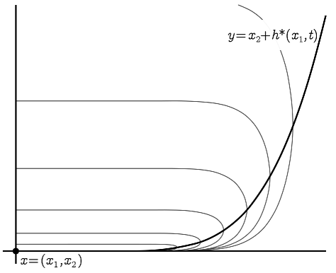
Figure 7.1. The graph of $h^{\ast}$ for $x_{1}>0$ small.

Then in the case $r_{k}\geq\frac{1}{\left|F^{\prime}\left(x_{1}\right)\right|}$, we have $h^{\ast}\left(x_{1},r_{k+1}\right)=h\left(x_{1},r_{k}\right)$, $k\geq 0$, where $h\left(x_{1},r_{k}\right)$ is the height of $B\left(x,r_{k}\right)$ as defined in Proposition 38. In the opposite case $r_{k}<\frac{1}{\left|F^{\prime}\left(x_{1}\right)\right|}$, we have $r_{k+1}=\frac{1}{2}r_{k}$ instead, and we will estimate differently.

For $k\geq 0$ define

$$E\left(x,r_{k}\right)$$

$$\equiv\left\{\begin{array}[]{l}\left\{y:x_{1}+r_{k+1}\leq y_{1}<x_{1}+r_{k},~{}\left|y_{2}\right|<h^{\ast}\left(x_{1},y_{1}-x_{1}\right)\right\},\text{ if }r_{k}\geq\frac{1}{\left|F^{\prime}\left(x_{1}\right)\right|}\\ \left\{y:x_{1}+r_{k+1}\leq y_{1}<x_{1}+r_{k},~{}\left|y_{2}\right|<h^{\ast}\left(x_{1},r_{k}^{\ast}\right)=h\left(x_{1},r_{k}\right)\right\},\text{ if }r_{k}<\frac{1}{\left|F^{\prime}\left(x_{1}\right)\right|}\end{array}\right.$$

where we have written $r_{k}^{\ast}=r^{\ast}\left(x_{1},r_{k}\right)$ for convenience. We claim that

(7.4) $$\left|E\left(x,r_{k}\right)\right|\approx\left|E\left(x,r_{k}\right)\bigcap B\left(x,r_{k}\right)\right|\approx\left|B\left(x,r_{k}\right)\right|\text{ for all }k\geq 1.$$

Indeed, in the first case $r_{k}\geq\frac{1}{\left|F^{\prime}\left(x_{1}\right)\right|}$, the second set of inequalities follows immediately by Corollary 44, and since $E\left(x,r_{k}\right)\subset B\left(x,r_{k-1}\right)$ we have that

$$\left|E\left(x,r_{k}\right)\bigcap B\left(x,r_{k}\right)\right| \leq \left|E\left(x,r_{k}\right)\right|\leq\left|B\left(x,r_{k-1}\right)\right|$$

$$\lesssim \left|B\left(x,r_{k}\right)\right|\lesssim\left|E\left(x,r_{k}\right)\bigcap B\left(x,r_{k}\right)\right|,$$

which establishes the first set of inequalities in (7.4). In the second case $r_{k}<\frac{1}{\left|F^{\prime}\left(x_{1}\right)\right|}$, we have

$$\left|E\left(x,r_{k}\right)\right|=\frac{1}{2}r_{k}h^{\ast}\left(x_{1},r_{k}^{\ast}\right)\approx\left(r_{k}-r_{k}^{\ast}\right)h\left(x_{1},r_{k}^{\ast}\right)\approx\left|B\left(x,r_{k}\right)\right|,$$

and from (6.15) with $\left(x,y\right)\in\partial B\left(x,r_{k}\right)$, we have

$$y\geq f\left(x\right)\left(r_{k}-x+x_{1}\right)\approx f\left(x_{1}\right)r_{k},$$

for all $x\in\left[x_{1},x_{1}+r\right]$ since we are in the case $r_{k}<\frac{1}{\left|F^{\prime}\left(x_{1}\right)\right|}$. It follows that

$$E\left(x,r_{k}\right)\cap B\left(x,r_{k}\right)\supset\left[x_{1}+\frac{r_{k}}{2},x_{1}+\frac{3r_{k}}{4}\right]\times\left[-cf\left(x_{1}\right)r_{k},cf\left(x_{1}\right)r_{k}\right]$$

and hence that

$$\left|E\left(x,r_{k}\right)\cap B\left(x,r_{k}\right)\right|\geq\frac{1}{2}cr_{k}f\left(x_{1}\right)r_{k}\approx\left|B\left(x,r_{k}\right)\right|\geq\left|E\left(x,r_{k}\right)\cap B\left(x,r_{k}\right)\right|.$$

This completes the proof of (7.4).

Now define $\Gamma\left(x,r\right)$ to be the set

$$\Gamma\left(x,r\right)=\bigcup\limits_{k=1}^{\infty}\mathop{\mathrm{c}o}\left[E\left(x,r_{k}\right)\cup E\left(x,r_{k+1}\right)\right],$$

where $\mathop{\mathrm{c}o}E$ denotes the convex hull of the set $E$. Set

$$\mathbb{E}_{x,r_{1}}w\equiv\frac{1}{\left|E(x,r_{1})\right|}\int\int_{E(x,r_{1})}w.$$

Lemma 49.

With $\Gamma\left(x,r\right)$, $E\left(x,r_{1}\right)$ and $\mathbb{E}_{x,r_{1}}$ as above, and in particular with $r_{0}=r$ and $r_{1}$ given by (7.1), we have the subrepresentation formula

(7.5) $$\left|w\left(x\right)-\mathbb{E}_{x,r_{1}}w\right|\leq C\int_{\Gamma\left(x,r\right)}\left|\nabla_{A}w\left(y\right)\right|\frac{\widehat{d}\left(x,y\right)}{\left|B\left(x,d\left(x,y\right)\right)\right|}dy,$$

where $\nabla_{A}$ is as in (1.3) and

(7.6) $$\widehat{d}\left(x,y\right)\equiv\min\left\{d\left(x,y\right),\frac{1}{\left|F^{\prime}\left(x_{1}+d\left(x,y\right)\right)\right|}\right\}.$$

Note that when $f\left(r\right)=r^{N}$ is finite type, then $\widehat{d}\left(x,y\right)\approx d\left(x,y\right)$.

Proof.

Recall the sequence $\left\{r_{k}\right\}_{k=1}^{\infty}$ of decreasing radii above. Then since $w$ is a priori Lipschitz continuous, we can write,

$$w\left(x\right)- \mathbb{E}_{x,r_{1}}w$$

$$=\lim_{k\rightarrow\infty}\frac{1}{\left|E\left(x,r_{k}\right)\right|}\int_{E\left(x,r_{k}\right)}w\left(y\right)dy-\frac{1}{\left|E(x,r_{1})\right|}\int_{E(x,r_{1})}w$$

$$=\sum_{k=1}^{\infty}\left\{\frac{1}{\left|E\left(x,r_{k+1}\right)\right|}\int_{E\left(x,r_{k+1}\right)}w\left(y\right)dy-\frac{1}{\left|E\left(x,r_{k}\right)\right|}\int_{E\left(x,r_{k}\right)}w\left(z\right)dz\right\},$$

and so we have

$$\left|w\left(x\right)-\mathbb{E}_{x,r_{1}}w\right|$$

$$\lesssim \sum_{k=1}^{\infty}\frac{1}{\left|B\left(x,r_{k}\right)\right|^{2}}\int_{E\left(x,r_{k+1}\right)\times E\left(x,r_{k}\right)}\left|w\left(y\right)-w\left(z\right)\right|dydz$$

$$\lesssim \sum_{k=1}^{\infty}\frac{1}{\left|B\left(x,r_{k}\right)\right|^{2}}\int_{E\left(x,r_{k+1}\right)\times E\left(x,r_{k}\right)}$$

$$\ \ \ \ \ \ \ \ \ \ \times\left\{\left|w\left(y_{1},y_{2}\right)-w\left(z_{1},y_{2}\right)\right|+\left|w\left(z_{1},y_{2}\right)-w\left(z_{1},z_{2}\right)\right|\right\}dydz$$

$$\lesssim \sum_{k=1}^{\infty}\frac{1}{\left|B\left(x,r_{k}\right)\right|^{2}}\int_{E\left(x,r_{k+1}\right)\times E\left(x,r_{k}\right)}\int_{y_{1}}^{z_{1}}\left|w_{x}\left(s,y_{2}\right)\right|dsdy_{1}dy_{2}dz_{1}dz_{2}$$

$$+ \sum_{k=1}^{\infty}\frac{1}{\left|B\left(x,r_{k}\right)\right|^{2}}\int_{E\left(x,r_{k+1}\right)\times E\left(x,r_{k}\right)}\int_{y_{2}}^{z_{2}}\left|w_{y}\left(z_{1},t\right)\right|dtdy_{1}dy_{2}dz_{1}dz_{2}\ ,$$

which, with $H_{k}\left(x\right)\equiv E\left(x,r_{k+1}\right)\bigcup E\left(x,r_{k}\right)$, is dominated by

$$\sum_{k=1}^{\infty}\frac{1}{\left|B\left(x,r_{k}\right)\right|^{2}}\left(\int_{H_{k}\left(x\right)}\left|\nabla_{A}w\left(s,y_{2}\right)\right|dsdy_{2}\right)\left\{r_{k}-r_{k+1}\right\}\int_{H_{k}\left(x\right)}dz_{1}dz_{2}$$

$$+\sum_{k=1}^{\infty}\frac{1}{\left|B\left(x,r_{k}\right)\right|^{2}}\left(\int_{H_{k}\left(x\right)}\left|\nabla_{A}w\left(z_{1},t\right)\right|dz_{1}dt\right)\ \frac{h_{k}}{f\left(x_{1}+r_{k+1}\right)}\ \int_{H_{k}\left(x\right)}dy_{1}dy_{2}\ ,$$

where for the last term we used that

$$\left|w_{y}\left(z_{1},t\right)\right| = \frac{f(z_{1})}{f(z_{1})}\left|w_{y}\left(z_{1},t\right)\right|\leq\frac{1}{f(z_{1})}\left|\nabla_{A}w\left(z_{1},t\right)\right|$$

$$\leq \frac{1}{f(x_{1}+r_{k+1})}\left|\nabla_{A}w\left(z_{1},t\right)\right|\quad\forall(z_{1},z_{2})\in E(x,r_{k}).$$

Next, recall from Lemma 39 that $h_{k}\approx(r_{k}-r_{k+1})\cdot f(x_{1}+r_{k+1})$ by our choice of $r_{k+1}$ in (7.1). Moreover, by the estimates above we have that $|H_{k}(x)|\approx|B(x,r_{k})|,$ and

(7.7) $$\left|w\left(x\right)-\mathbb{E}_{x,r_{1}}w\right| \lesssim \sum_{k=1}^{\infty}\frac{r_{k}-r_{k+1}}{\left|B\left(x,r_{k}\right)\right|}\left(\int_{H_{k}\left(x\right)}\left|\nabla_{A}w\left(s,y_{2}\right)\right|dsdy_{2}\right)$$

$$\lesssim \int_{\Gamma(x,r)}\left|\nabla_{A}w\left(y\right)\right|\left(\sum_{k=1}^{\infty}\frac{r_{k}-r_{k+1}}{\left|B\left(x,r_{k}\right)\right|}\mathbf{1}_{E\left(x,r_{k}\right)}\left(y\right)\right)dy.$$

To make further estimates we need to consider two regions separately, namely;

1. $d(x,y)\geq\frac{1}{|F^{\prime}(x_{1})|}$. In this case we have

   $$r_{k}>d(x,y)\geq\frac{1}{|F^{\prime}(x_{1})|},$$

   which implies by Proposition 38 and (6.12)

   $$r_{k}-r_{k+1}\approx\frac{1}{|F^{\prime}(x_{1}+r_{k})|}\approx\frac{1}{|F^{\prime}(x_{1}+r_{k+2})|}<\frac{1}{|F^{\prime}(x_{1}+d(x,y))|}.$$

   Therefore, we are left with

   (7.8) $$\left|w\left(x\right)-\mathbb{E}_{x,r_{1}}w\right|$$

   $$\lesssim \int_{\Gamma(x,r)}\left|\nabla_{A}w\left(y\right)\right|\frac{1}{|F^{\prime}(x_{1}+d(x,y))|}\sum_{k:r_{k+1}<d(x,y)<r_{k}}\frac{1}{\left|B\left(x,r_{k}\right)\right|}dy$$

   $$\approx \int_{\Gamma(x,r)}\left|\nabla_{A}w\left(y\right)\right|\frac{1}{|F^{\prime}(x_{1}+d(x,y))|}\frac{1}{|B(x,d(x,y))|}dy.$$

2. $d(x,y)<\frac{1}{|F^{\prime}(x_{1})|}$. We can write

   $$\sum_{k:r_{k+1}<d(x,y)<r_{k}}\frac{r_{k}-r_{k+1}}{\left|B\left(x,r_{k}\right)\right|}\leq\sum_{k:r_{k+1}<d(x,y)<r_{k}}\frac{r_{k}}{\left|B\left(x,r_{k}\right)\right|}\lesssim\frac{d(x,y)}{|B(x,d(x,y))|},$$

   which gives

   (7.9) $$\left|w\left(x\right)-\mathbb{E}_{x,r_{1}}w\right|\lesssim\int_{\Gamma(x,r)}\left|\nabla_{A}w\left(y\right)\right|\frac{d(x,y)}{|B(x,d(x,y))|}.$$

To finish the proof we need to dominate the right hand sides of (7.8) and (7.9) with

(7.10) $$\int_{\Gamma(x,r)}\left|\nabla_{A}w\left(y\right)\right|\frac{\widehat{d}(x,y)}{|B(x,d(x,y))|}$$

where $\widehat{d}\left(x,y\right)=\min\left\{d\left(x,y\right),\frac{1}{\left|F^{\prime}\left(x_{1}+d\left(x,y\right)\right)\right|}\right\}$ in cases $1$ and $2$ respectively.

Suppose first that $d(x,y)\geq\frac{1}{|F^{\prime}(x_{1}+d(x,y))|}$. Since $|F^{\prime}(x_{1})|$ is a decreasing function of $x_{1}$ we have $d(x,y)\geq\frac{1}{|F^{\prime}(x_{1})|}$ and therefore we are in case 1 and (7.10) then follows from $\frac{1}{|F^{\prime}(x_{1}+d(x,y))|}=\widehat{d}(x,y)$.

If the reverse inequality holds, namely $d(x,y)<\frac{1}{|F^{\prime}(x_{1}+d(x,y))|}$, we have to consider two subcases. First, if $d(x,y)\leq\frac{1}{|F^{\prime}(x_{1})|}$, then we are in case 2 and (7.10) then follows from $d(x,y)=\widehat{d}(x,y)$. Finally, if

$$\frac{1}{|F^{\prime}(x_{1})|}\leq d(x,y)<\frac{1}{|F^{\prime}(x_{1}+d(x,y))|},$$

we are back in case 1, but by Proposition 38 we have

$$\frac{1}{|F^{\prime}(x_{1}+d(x,y))|}\approx d(x,y)-d(x,y)^{\ast}<d(x,y),$$

and again (7.10) holds since $d(x,y)=\widehat{d}(x,y)$.    

As a simple corollary we obtain a connection between $\widehat{d}(x,y)$ and the ‘width’ of the thickest part of a ball of radius $d(x,y)$, namely $d(x,y)-d^{\ast}(x,y)$, where if $r=d(x,y)$ and $r^{\ast}$ is as defined at the beginning of Subsection 6.3.4 of Chapter 7, then we define $d^{\ast}(x,y)$ by

(7.11) $$d^{\ast}(x,y)\equiv r^{\ast}.$$

Note that if $x$ and $r$ are fixed, then for every $y\in\partial B\left(x,r\right)$ we have $d(x,y)-d^{\ast}(x,y)=r-r^{\ast}$.

Corollary 50.

Let $d(x,y)>0$ be the distance between any two points $x,y\in\Omega$ and let $d^{\ast}(x,y)$ be as in (7.11), and $\widehat{d}(x,y)$ be as defined in (7.6) of Lemma 49. Then

$$\widehat{d}(x,y)\approx d(x,y)-d^{\ast}(x,y)$$

Proof.

As before, we consider two cases

1. $d(x,y)\geq\frac{1}{|F^{\prime}(x_{1})|}$. In this case we have from Proposition 38

   $$d(x,y)-d^{\ast}(x,y)\approx\frac{1}{|F^{\prime}(x_{1}+d(x,y))|}.$$

   If $d(x,y)\geq\frac{1}{|F^{\prime}(x_{1}+d(x,y))|}$, then $\widehat{d}(x,y)=\frac{1}{|F^{\prime}(x_{1}+d(x,y))|}$ and the claim is proved. If, on the other hand,

   $$d(x,y)\leq\frac{1}{|F^{\prime}(x_{1}+d(x,y))|},$$

   then $\widehat{d}(x,y)=d(x,y)$ and

   $$d(x,y)>d(x,y)-d^{\ast}(x,y)\approx\frac{1}{|F^{\prime}(x_{1}+d(x,y))|}\geq d(x,y),$$

   and the claim follows.

2. $d(x,y)<\frac{1}{|F^{\prime}(x_{1})|}$. From Proposition 38 we have in this case

   $$d(x,y)-d^{\ast}(x,y)\approx d(x,y).$$

   From the monotonicity of the function $F^{\prime}(x)$ we have

   $$d(x,y)<\frac{1}{|F^{\prime}(x_{1})|}\leq\frac{1}{|F^{\prime}(x_{1}+d(x,y))|},$$

   and therefore $\widehat{d}(x,y)=d(x,y)\approx d(x,y)-d^{\ast}(x,y)$.

   

7.1.2. The higher dimensional case

The subrepresentation inequality here is similar to Lemma 49 in two dimensions, with the main differences being in the definition of the cusp-like region $\Gamma\left(x,r\right)$ in higher dimensions. On the one hand, the shape of the higher dimensional balls dictates the rough form of $\Gamma\left(x,r\right)$, but we will also need to redefine the sequence of radii $\left\{r_{k}\right\}_{k=1}^{\infty}$ used in the definition of $\Gamma\left(x,r\right)$. We begin by addressing the higher dimensional form, and later will turn to the new sequences $\left\{r_{k}\right\}_{k=1}^{\infty}$.

Recall that we denote points $x\in\mathbb{R}^{n}$ as

$$x=\left(x_{1},\mathbf{x}_{2},x_{3}\right)\in\mathbb{R}\times\mathbb{R}^{n-2}\times\mathbb{R\,}.$$

Let $\left|B\left(x,d\left(x,y\right)\right)\right|$ denote the $n$-dimensional Lebesgue measure of $B\left(x,d\left(x,y\right)\right)$ where $d\left(x,y\right)$ is now the $n$-dimensional control distance. We define the cusp-like region $\Gamma\left(x,r\right)$ and the ‘ends’ $E\left(x,r_{k}\right)$ of the balls $B\left(x,r_{k}\right)$ by

(7.12) $$\Gamma\left(x,r\right) = \bigcup\limits_{k=1}^{\infty}E\left(x,r_{k}\right);$$

(7.16) $$E\left(x,r_{k}\right) \equiv \left\{y=\left(y_{1},\mathbf{y}_{2},y_{3}\right):\begin{array}[]{c}r_{k+1}\leq y_{1}-x_{1}<r_{k}\\ \left|\mathbf{y}_{2}-\mathbf{x}_{2}\right|<\sqrt{r_{k}^{2}-\left(y_{1}-x_{1}\right)^{2}}\\ \left|y_{3}-x_{3}\right|<h^{\ast}\left(x_{1},y_{1}-x_{1}\right)\end{array}\right\},$$

where we recall

$$r_{k+1}=\left\{\begin{array}[]{lll}r^{\ast}\left(x_{1},r_{k}\right)&&\text{if }r_{k}\geq\frac{1}{\left|F^{\prime}\left(x_{1}\right)\right|}\\ \frac{1}{2}r_{k}&&\text{if }r_{k}<\frac{1}{\left|F^{\prime}\left(x_{1}\right)\right|}\end{array}\right.,$$

and where $r^{\ast}$ is defined in Definition 37 right before Proposition 38. We also define the modified ‘end’ $\widetilde{E}$ by

(7.17) $$\widetilde{E}\left(x,r_{k}\right)\equiv\left\{y=\left(y_{1},\mathbf{y}_{2},y_{3}\right):\begin{array}[]{c}r_{k+1}\leq y_{1}-x_{1}<r_{k}\\ \left|\mathbf{y}_{2}-\mathbf{x}_{2}\right|<\sqrt{r_{k}^{2}-r_{k+1}^{2}}\\ \left|y_{3}-x_{3}\right|<h^{\ast}\left(x_{1},r_{k}\right)\end{array}\right..$$

Note the estimate

(7.18) $$\left|\mathbf{y}_{2}-\mathbf{x}_{2}\right| < \sqrt{r_{k}^{2}-r_{k+1}^{2}}\approx\sqrt{r_{k}-r_{k+1}}\sqrt{r_{k}}$$

$$\text{for }y \in \widetilde{E}\left(x,r_{k}\right).$$

We claim the following lemma.

Lemma 51.

With notation as above we have

$$\left|\widetilde{E}\left(x,r_{k}\right)\right|\approx\left|E\left(x,r_{k}\right)\right|\approx\left|E\left(x,r_{k}\right)\cap B\left(x,r_{k}\right)\right|\approx\left|B\left(x,r_{k}\right)\right|.$$

Proof.

Recall that by Lemma 48 we have

(7.19) $$\left|B\left(x,r_{k}\right)\right|\approx\left\{\begin{array}[]{ccc}r_{k}^{n}f(x_{1})&\text{ if }&r_{k}\leq\frac{2}{\left|F^{\prime}\left(x_{1}\right)\right|}\\ \frac{f\left(x_{1}+r_{k}\right)}{\left|F^{\prime}\left(x_{1}+r_{k}\right)\right|^{n}}\left(r_{k}\left|F^{\prime}\left(x_{1}+r_{k}\right)\right|\right)^{\frac{n}{2}-1}&\text{ if }&r_{k}\geq\frac{2}{\left|F^{\prime}\left(x_{1}\right)\right|}\end{array}\right..$$

To show

(7.20) $$\left|E\left(x,r_{k}\right)\right|\approx\left|B\left(x,r_{k}\right)\right|$$

we first note that $\left|E\left(x,r_{k}\right)\right|\approx\left|\widetilde{E}\left(x,r_{k}\right)\right|$. Integrating, we easily obtain

$$|\widetilde{E}\left(x,r_{k}\right)|\approx h^{\ast}\left(x_{1},r_{k}\right)r_{k}^{\frac{n-2}{2}}(r_{k}-r_{k+1})^{\frac{n}{2}}.$$

Now, in the first case $r_{k}\geq\frac{1}{\left|F^{\prime}\left(x_{1}\right)\right|}$ we have by Proposition 38 $r_{k}-r_{k+1}=r_{k}-r_{k}^{\ast}\approx\frac{1}{\left|F^{\prime}\left(x_{1}+r_{k}\right)\right|}$ and

$$h^{\ast}\left(x_{1},r_{k}\right)=h^{\ast}\left(x_{1},r_{k-1}^{\ast}\right)=h(x_{1},r_{k-1})\approx\frac{f\left(x_{1}+r_{k-1}\right)}{\left|F^{\prime}\left(x_{1}+r_{k-1}\right)\right|}\approx\frac{f\left(x_{1}+r_{k}\right)}{\left|F^{\prime}\left(x_{1}+r_{k}\right)\right|},$$

where for the last set of inequalities we used $r_{k}=r_{k-1}^{\ast}$ and the estimate (6.12). This gives

$$|\widetilde{E}\left(x,r_{k}\right)|\approx r_{k}^{\frac{n}{2}-1}\frac{f\left(x_{1}+r_{k}\right)}{\left|F^{\prime}\left(x_{1}+r_{k}\right)\right|^{\frac{n}{2}+1}},$$

which is the second estimate in (7.19) provided we also have $r_{k}\geq\frac{2}{\left|F^{\prime}\left(x_{1}\right)\right|}$. Moreover, when $\frac{1}{\left|F^{\prime}\left(x_{1}\right)\right|}\leq r_{k}\leq\frac{2}{\left|F^{\prime}\left(x_{1}\right)\right|}$ the two estimates in (7.19) coincide, so we conclude (7.20) for $r_{k}\geq\frac{1}{\left|F^{\prime}\left(x_{1}\right)\right|}$.

In the second case $r_{k}<\frac{1}{\left|F^{\prime}\left(x_{1}\right)\right|}$ we have $r_{k}-r_{k+1}=\frac{r_{k}}{2}$ and using part (3) of Proposition 38

$$h^{\ast}\left(x_{1},r_{k}\right)\approx h^{\ast}\left(x_{1},r_{k+1}\right)=h(x_{1},r_{k})\approx r_{k}f(x_{1}),$$

which gives

$$|\widetilde{E}\left(x,r_{k}\right)|\approx r_{k}^{n}f(x_{1}).$$

This concludes the proof of (7.20).

We are thus left to show

(7.21) $$\left|E\left(x,r_{k}\right)\cap B\left(x,r_{k}\right)\right|\approx\left|B\left(x,r_{k}\right)\right|.$$

In the case $r_{k}\geq\frac{1}{\left|F^{\prime}\left(x_{1}\right)\right|}$ we have

$$E\left(x,r_{k}\right)\cap B\left(x,r_{k}\right)\supset B_{+}\left(x,r_{k}\right)\equiv\left\{\left(y_{1},\mathbf{y}_{2},y_{3}\right)\in B\left(x,r_{k}\right):y_{1}>x_{1}+r_{k}^{\ast}\right\}$$

and therefore

$$\left|E\left(x,r_{k}\right)\cap B\left(x,r_{k}\right)\right|\geq\left|B_{+}\left(x,r_{k}\right)\right|$$

$$\quad=\int\limits_{|\mathbf{y}_{2}|\leq r_{k}}\left|{B_{2D}}\left(\left(x_{1},\mathbf{0},0\right),\sqrt{r_{k}^{2}-\left|\mathbf{y}_{2}\right|^{2}}\right)\cap\{y_{1}-x_{1}>r_{k}^{*}\}\right|d\mathbf{y}_{2}$$

$$\quad\approx\int\limits_{|\mathbf{y}_{2}|\leq r_{k}}\left(\sqrt{r_{k}^{2}-\left|\mathbf{y}_{2}\right|^{2}}-r_{k}^{\ast}\right)_{+}\cdot h\left(x_{1},\sqrt{r_{k}^{2}-\left|\mathbf{y}_{2}\right|^{2}}\right)d\mathbf{y}_{2}$$

$$\quad\approx\int\limits_{|\mathbf{y}_{2}|\leq r_{k}}\left(\sqrt{r^{2}-\left|\mathbf{y}_{2}\right|^{2}}-r_{k}^{\ast}\right)_{+}\cdot\frac{f\left(x_{1}+\sqrt{r_{k}^{2}-\left|\mathbf{y}_{2}\right|^{2}}\right)}{\left|F^{\prime}\left(x_{1}+\sqrt{r^{2}-\left|\mathbf{y}_{2}\right|^{2}}\right)\right|}d\mathbf{y}_{2}$$

$$\quad=\int\limits_{|\mathbf{y}_{2}|^{2}\leq r_{k}^{2}-{r_{k}^{\ast}}^{2}}\left(\sqrt{r_{k}^{2}-\left|\mathbf{y}_{2}\right|^{2}}-r_{k}^{\ast}\right)\cdot\frac{f\left(x_{1}+\sqrt{r^{2}-\left|\mathbf{y}_{2}\right|^{2}}\right)}{\left|F^{\prime}\left(x_{1}+\sqrt{r_{k}^{2}-\left|\mathbf{y}_{2}\right|^{2}}\right)\right|}d\mathbf{y}_{2}$$

$$\quad\approx\frac{f(x_{1}+r_{k})}{|F^{\prime}(x_{1}+r_{k})|}\int\limits_{|\mathbf{y}_{2}|^{2}\leq r_{k}^{2}-{r_{k}^{\ast}}^{2}}\left(\sqrt{r_{k}^{2}-\left|\mathbf{y}_{2}\right|^{2}}-r_{k}^{\ast}\right)d\mathbf{y}_{2},$$

where for the last equality we used (6.12). Passing to the polar coordinates, $\rho=\left|\mathbf{y}_{2}\right|$, we have

$$\int\limits_{|\mathbf{y}_{2}|^{2}\leq r_{k}^{2}-{r_{k}^{\ast}}^{2}}\left(\sqrt{r_{k}^{2}-\left|\mathbf{y}_{2}\right|^{2}}-r_{k}^{\ast}\right)d\mathbf{y}_{2} \approx\int\limits_{0}^{\sqrt{r_{k}^{2}-{r_{k}^{\ast}}^{2}}}\left(\sqrt{r_{k}^{2}-\rho^{2}}-r_{k}^{\ast}\right)\rho^{n-3}d\rho$$

$$\geq\int\limits_{0}^{\sqrt{r_{k}^{2}-\frac{1}{4}(r_{k}+r_{k}^{\ast})^{2}}}\left(\sqrt{r_{k}^{2}-\rho^{2}}-r_{k}^{\ast}\right)\rho^{n-3}d\rho$$

$$\geq\frac{1}{2}(r_{k}-r_{k}^{\ast})\int\limits_{0}^{\sqrt{r_{k}^{2}-\frac{1}{4}(r_{k}+r_{k}^{\ast})^{2}}}\rho^{n-3}d\rho$$

$$\approx(r_{k}-r_{k}^{\ast})^{\frac{n}{2}}r^{\frac{n}{2}-1}$$

$$\approx(r_{k}-r_{k}^{\ast})^{\frac{n}{2}}r_{k}^{\frac{n}{2}-1}.$$

Using part (2) of Proposition 38 we have $r_{k}-r_{k}^{\ast}\approx 1/|F^{\prime}(x_{1}+r_{k})|$ and therefore

$$\left|E\left(x,r_{k}\right)\cap B\left(x,r_{k}\right)\right|\gtrsim\frac{f(x_{1}+r_{k})}{|F^{\prime}(x_{1}+r_{k})|^{\frac{n}{2}+1}}r^{\frac{n}{2}-1}\approx\left|B\left(x,r_{k}\right)\right|.$$

Finally, in the case $r_{k}<\frac{1}{\left|F^{\prime}\left(x_{1}\right)\right|}$, proceeding exactly as in the proof of (7.4) in the $2$-dimensional case, we can show

$$E\left(x,r_{k}\right)\cap B\left(x,r_{k}\right)\supset\left[x_{1}+\frac{r_{k}}{2},x_{1}+\frac{3r_{k}}{4}\right]\times\left\{|\mathbf{y}_{2}|\leq\frac{r_{k}}{2}\right\}\times\left[-cf\left(x_{1}\right)r_{k},cf\left(x_{1}\right)r_{k}\right]$$

and thus

$$\left|E\left(x,r_{k}\right)\cap B\left(x,r_{k}\right)\right|\gtrsim r_{k}^{n}f(x_{1})\approx\left|B\left(x,r_{k}\right)\right|.$$

This concludes the proof of (7.21), and therefore the proof of Lemma 51.    

The difficulty with the standard sequence of radii

Recall that we began the proof of Lemma 49 in two dimensions by subtracting consecutive averages of $w$ over the ends $E\left(x,r_{k}\right)$ and $E\left(x,r_{k+1}\right)$ to obtain

$$w\left(x\right)- \mathbb{E}_{x,r_{1}}w$$

$$=\lim_{k\rightarrow\infty}\frac{1}{\left|E\left(x,r_{k}\right)\right|}\int_{E\left(x,r_{k}\right)}w\left(y\right)dy-\mathbb{E}_{x,r_{1}}w$$

$$=\sum_{k=1}^{\infty}\left\{\frac{1}{\left|E\left(x,r_{k+1}\right)\right|}\int_{E\left(x,r_{k+1}\right)}w\left(y\right)dy-\frac{1}{\left|E\left(x,r_{k}\right)\right|}\int_{E\left(x,r_{k}\right)}w\left(z\right)dz\right\}.$$

If we simply proceed in this way in higher dimensions we will obtain, just as in the two dimensional proof, that

$$\left|w\left(x\right)-\mathbb{E}_{x,r_{1}}w\right|$$

$$\quad\lesssim\sum_{k=1}^{\infty}\frac{1}{\left|B\left(x,r_{k}\right)\right|^{2}}\int\limits_{E\left(x,r_{k+1}\right)\times E\left(x,r_{k}\right)}\left|w\left(y\right)-w\left(z\right)\right|dydz$$

$$\quad\lesssim\sum_{k=1}^{\infty}\frac{1}{\left|B\left(x,r_{k}\right)\right|^{2}}\int\limits_{E\left(x,r_{k+1}\right)\times E\left(x,r_{k}\right)}\left|w\left(y_{1},\mathbf{y}_{2},y_{3}\right)-w\left(z_{1},\mathbf{y}_{2},y_{3}\right)\right|dydz$$

$$\quad\quad+\sum_{k=1}^{\infty}\frac{1}{\left|B\left(x,r_{k}\right)\right|^{2}}\int\limits_{E\left(x,r_{k+1}\right)\times E\left(x,r_{k}\right)}\left|w\left(z_{1},\mathbf{y}_{2},y_{3}\right)-w\left(z_{1},\mathbf{z}_{2},y_{3}\right)\right|dydz$$

$$\quad\quad+\sum_{k=1}^{\infty}\frac{1}{\left|B\left(x,r_{k}\right)\right|^{2}}\int\limits_{E\left(x,r_{k+1}\right)\times E\left(x,r_{k}\right)}\left|w\left(z_{1},\mathbf{z}_{2},y_{3}\right)-w\left(z_{1},\mathbf{z}_{2},z_{3}\right)\right|dydz$$

$$\quad\equiv I+II+III,$$

but where now

$$I\lesssim\sum_{k=1}^{\infty}\frac{1}{\left|B\left(x,r_{k}\right)\right|^{2}}\int\limits_{E\left(x,r_{k+1}\right)\times E\left(x,r_{k}\right)}\int_{y_{1}}^{z_{1}}\left|w_{x_{1}}\left(s,\mathbf{y}_{2},y_{3}\right)\right|dsdy_{1}d\mathbf{y}_{2}dy_{3}dz_{1}d\mathbf{z}_{2}dz_{3}\ ,$$

and

$$II\lesssim \sum_{k=1}^{\infty}\frac{1}{\left|B\left(x,r_{k}\right)\right|^{2}}\int\limits_{E\left(x,r_{k+1}\right)\times E\left(x,r_{k}\right)}\int_{0}^{1}\left|\left(\mathbf{z}_{2}-\mathbf{y}_{2}\right)\cdot\nabla_{\mathbf{x}_{2}}w\left(z_{1},t\mathbf{z}_{2}+\left(1-t\right)\mathbf{y}_{2},y_{3}\right)\right|$$

$$\ \ \ \ \ \ \ \ \ \ \ \ \ \ \ \ \ \ \ \ \ \ \ \ \ \ \ \ \ \ \ \ \ \ \ \ \ \ \ \ \ \ \ \ \ \ \ \ \ \ \ \ \ \ \ \ \ \times dtdy_{1}d\mathbf{y}_{2}dy_{3}dz_{1}d\mathbf{z}_{2}dz_{3}\ ,$$

and

$$III\lesssim\sum_{k=1}^{\infty}\frac{1}{\left|B\left(x,r_{k}\right)\right|^{2}}\int\limits_{E\left(x,r_{k+1}\right)\times E\left(x,r_{k}\right)}\int_{y_{3}}^{z_{3}}\left|w_{x_{3}}\left(z_{1},\mathbf{z}_{2},u\right)\right|dudy_{1}d\mathbf{y}_{2}dy_{3}dz_{1}d\mathbf{z}_{2}dz_{3}\ .$$

Thus with $\bigtriangleup r_{k}\equiv r_{k}-r_{k+1}$, we have

$$I \lesssim\sum_{k=1}^{\infty}\frac{\bigtriangleup r_{k}}{\left|B\left(x,r_{k}\right)\right|}\int_{H\left(x,r_{k}\right)}\left|w_{x_{1}}\left(s,\mathbf{y}_{2},y_{3}\right)\right|dsd\mathbf{y}_{2}dy_{3}$$

$$\lesssim\sum_{k=1}^{\infty}\frac{\bigtriangleup r_{k}}{\left|B\left(x,r_{k}\right)\right|}\int_{H\left(x,r_{k}\right)}\left|\nabla_{A}w\right|,$$

and an easy computation also shows that

$$III\lesssim\sum_{k=1}^{\infty}\frac{\bigtriangleup r_{k}}{\left|B\left(x,r_{k}\right)\right|}\int_{H\left(x,r_{k}\right)}\left|\nabla_{A}w\right|,$$

which for terms $I$ and $III$ delivers the good estimate (7.7) in the $2$-dimensional proof above. But upon using the inequality $\left|\mathbf{y}_{2}-\mathbf{x}_{2}\right|\lesssim\sqrt{r_{k}-r_{k+1}}\sqrt{r_{k}}$ from (7.18), the corresponding estimate for $II$ is

$$II\lesssim\sum_{k=1}^{\infty}\frac{\sqrt{r_{k}\bigtriangleup r_{k}}}{\left|B\left(x,r_{k}\right)\right|}\int_{H\left(x,r_{k}\right)}\left|\nabla_{A}w\right|,$$

which is much too large as $\sqrt{r_{k}\bigtriangleup r_{k}}\gg\bigtriangleup r_{k}$ when $\bigtriangleup r_{k}\ll r_{k}$.

This suggests that we hold the variable $\mathbf{y}_{2}$ fixed, and take the difference of lower dimensional averages, and then average over $\mathbf{y}_{2}$. But this will require additional information on the regularity of the sequence of radii $\left\{r_{k}\right\}_{k=1}^{\infty}$, something we cannot easily derive from the current definition of $r_{k}$. So we now turn to redefining the sequence of radii to be used in our subrepresentation inequalities.

Geometric estimates

We will estimate the differences of the quantities

(7.22) $$q_{k}\equiv\sqrt{r_{k}^{2}-r_{k+1}^{2}}$$

appearing as the widths of the modified ends $\widetilde{E}\left(x_{1},r_{k}\right)$ defined in (7.17). First recall that there are positive constants $c,C$ such that

$$c\leq\left(r_{k}-r_{k+1}\right)\left|F^{\prime}\left(x_{1}+r_{k}\right)\right|\leq C,\ \ \ \ \ \text{for }r_{k}\geq\frac{2}{\left|F^{\prime}\left(x_{1}\right)\right|}.$$

In view of this, let us redefine, for each $\gamma>0$, the sequence $\left\{r_{k}\right\}_{k=0}^{\infty}$ recursively by demanding that the first inequality above be an equality.

Definition 52.

For $\gamma>0$ set

(7.23) $$r_{k+1}^{\gamma}\equiv\left\{\begin{array}[]{ccc}r_{k}^{\gamma}-\frac{\gamma}{\left|F^{\prime}\left(x_{1}+r_{k}\right)\right|}&\text{ if }&r_{k}^{\gamma}\geq\frac{\gamma}{\left|F^{\prime}\left(x_{1}\right)\right|}\\ \frac{1}{2}r_{k}^{\gamma}&\text{ if }&r_{k}^{\gamma}<\frac{\gamma}{\left|F^{\prime}\left(x_{1}\right)\right|}\end{array}\right.,\ \ \ \ \ k\geq 0.$$

We will typically suppress the superscript $\gamma$ and continue to write $r_{k}$ in place of $r_{k}^{\gamma}$ when $\gamma$ is understood. With this revised definition of the sequence of radii, and the corresponding balls and ends, we retain the two-dimensional volume estimates and the subrepresentation inequality in Lemma 49, with perhaps larger constants of comparability. These details are easily verified and left for the reader.

Now, continuing to suppress $\gamma$, let

$$\bigtriangleup r_{k}\equiv r_{k}-r_{k+1}\text{ and }\bigtriangleup^{2}r_{k}\equiv\bigtriangleup r_{k}-\bigtriangleup r_{k+1}\text{ and }\bigtriangleup q_{k}\equiv q_{k}-q_{k+1}$$

denote the first and second order differences of the sequences $\left\{r_{k}\right\}_{k=0}^{\infty}$ and $\left\{q_{k}\right\}_{k=0}^{\infty}$. The point of the new definitions of the sequence $\left\{r_{k}^{\gamma}\right\}_{k=0}^{\infty}$ is to obtain a good estimate on its second order differences $\bigtriangleup^{2}r_{k}^{\gamma}$, and hence also on the first order differences of $\left\{q_{k}^{\gamma}\right\}_{k=0}^{\infty}$.

Lemma 53.

With $\gamma>0$ and the sequence $\left\{r_{k}^{\gamma}\right\}_{k=0}^{\infty}$ defined as in (7.23), and $\left\{q_{k}^{\gamma}\right\}_{k=0}^{\infty}$ defined as in (7.22), we have the following estimates:

$$\bigtriangleup r_{k}^{\gamma} = \left\{\begin{array}[]{ccc}\frac{\gamma}{\left|F^{\prime}\left(x_{1}+r_{k}\right)\right|}&\text{ if }&r_{k}\geq\frac{\gamma}{\left|F^{\prime}\left(x_{1}\right)\right|}\\ \frac{1}{2}r_{k}&\text{ if }&r_{k}<\frac{\gamma}{\left|F^{\prime}\left(x_{1}\right)\right|}\end{array}\right.,$$

$$\bigtriangleup^{2}r_{k}^{\gamma} \approx \frac{\left[\bigtriangleup r_{k}\right]^{2}}{r_{k}},$$

$$q_{k}^{\gamma} \approx \sqrt{r_{k}\bigtriangleup r_{k}},$$

$$\bigtriangleup q_{k}^{\gamma} \lesssim \bigtriangleup r_{k},$$

where the implied constants of comparability depend on $\gamma>0$.

Proof.

We suppress the superscript $\gamma$ and prove only the case where $r_{k}\geq\frac{\gamma}{\left|F^{\prime}\left(x_{1}\right)\right|}$, since in the opposite case where $r_{k+1}=\frac{1}{2}r_{k}$ and $\bigtriangleup r_{k}=\frac{1}{2}r_{k}$, the estimates then follow immediately. We begin with

$$\bigtriangleup^{2}r_{k} = \bigtriangleup r_{k}-\bigtriangleup r_{k+1}=\frac{\gamma}{\left|F^{\prime}\left(x_{1}+r_{k}\right)\right|}-\frac{\gamma}{\left|F^{\prime}\left(x_{1}+r_{k+1}\right)\right|}$$

$$= \gamma\frac{F^{\prime}\left(x_{1}+r_{k}\right)-F^{\prime}\left(x_{1}+r_{k+1}\right)}{\left|F^{\prime}\left(x_{1}+r_{k}\right)\right|\left|F^{\prime}\left(x_{1}+r_{k+1}\right)\right|}$$

$$= \gamma\frac{F^{\prime\prime}\left(x_{1}+\left(1-\theta\right)r_{k}+\theta r_{k+1}\right)\ \left(r_{k}-r_{k+1}\right)}{\left|F^{\prime}\left(x_{1}+r_{k}\right)\right|\left|F^{\prime}\left(x_{1}+r_{k+1}\right)\right|}$$

$$\approx \frac{\frac{\left|F^{\prime}\left(x_{1}+\left(1-\theta\right)r_{k}+\theta r_{k+1}\right)\right|}{x_{1}+\left(1-\theta\right)r_{k}+\theta r_{k+1}}\left(r_{k}-r_{k+1}\right)}{\left|F^{\prime}\left(x_{1}+r_{k}\right)\right|\left|F^{\prime}\left(x_{1}+r_{k+1}\right)\right|}\lesssim\frac{\left[\bigtriangleup r_{k}\right]^{2}}{r_{k+1}},$$

where the last two line follows from our assumptions on $F$ and (7.23). Next we have

$$q_{k}=\sqrt{r_{k}-r_{k+1}}\sqrt{r_{k}+r_{k+1}}\approx\sqrt{r_{k}\bigtriangleup r_{k}},$$

and finally we have

$$\bigtriangleup q_{k} = \sqrt{\bigtriangleup r_{k}}\sqrt{r_{k}+r_{k+1}}-\sqrt{\bigtriangleup r_{k+1}}\sqrt{r_{k+1}+r_{k+2}}$$

$$= \left(\sqrt{\bigtriangleup r_{k}}-\sqrt{\bigtriangleup r_{k+1}}\right)\sqrt{r_{k}+r_{k+1}}$$

$$+\sqrt{\bigtriangleup r_{k+1}}\left(\sqrt{r_{k}+r_{k+1}}-\sqrt{r_{k+1}+r_{k+2}}\right)$$

$$\equiv I+II.$$

Now

$$I \approx \left(\sqrt{\bigtriangleup r_{k}}-\sqrt{\bigtriangleup r_{k+1}}\right)\sqrt{r_{k}}\approx\left(\frac{\bigtriangleup r_{k}-\bigtriangleup r_{k+1}}{\sqrt{\bigtriangleup r_{k}}+\sqrt{\bigtriangleup r_{k+1}}}\right)\sqrt{r_{k}}$$

$$\approx \left(\bigtriangleup^{2}r_{k}\right)\sqrt{\frac{r_{k}}{\bigtriangleup r_{k}}}\lesssim\frac{\left[\bigtriangleup r_{k}\right]^{2}}{r_{k+1}}\sqrt{\frac{r_{k}}{\bigtriangleup r_{k}}}=\frac{r_{k}}{r_{k+1}}\sqrt{\frac{\bigtriangleup r_{k}}{r_{k}}}\bigtriangleup r_{k}\lesssim\bigtriangleup r_{k}$$

and

$$II = \sqrt{\bigtriangleup r_{k+1}}\frac{\left(r_{k}+r_{k+1}\right)-\left(r_{k+1}+r_{k+2}\right)}{\sqrt{r_{k}+r_{k+1}}+\sqrt{r_{k+1}+r_{k+2}}}$$

$$\approx \sqrt{\frac{\bigtriangleup r_{k+1}}{r_{k}}}\bigtriangleup r_{k}\lesssim\bigtriangleup r_{k}\ .$$

   

Statements of subrepresentation inequalities

Set

$$\mathbb{E}_{x,r_{1}}w\equiv\frac{1}{\left|E(x,r_{1})\right|}\int_{E(x,r_{1})}w.$$

Lemma 54 ($n$D subrepresentation).

With $\Gamma\left(x,r\right)$ as above, and $r_{0}=r$ and $r_{1}$ given by (7.1), we have the subrepresentation formula

$$\left|w\left(x\right)-\mathbb{E}_{x,r_{1}}w\right|\leq C\int_{\Gamma\left(x,r\right)}\left|\nabla_{A}w\left(y\right)\right|\frac{\widehat{d}\left(x,y\right)}{\left|B\left(x,d\left(x,y\right)\right)\right|}dy,$$

where $\nabla_{A}$ is as in (1.3) and

$$\widehat{d}\left(x,y\right)\equiv\min\left\{d\left(x,y\right),\frac{1}{\left|F^{\prime}\left(x_{1}+d\left(x,y\right)\right)\right|}\right\}.$$

We next claim that the subrepresentation inequality continues to hold if we use the modified ‘end’ $\widetilde{E}\left(x,r_{k}\right)$ in (7.17) to define a modified cusp-like region

(7.25) $$\widetilde{\Gamma}\left(x,r\right)=\bigcup\limits_{k=1}^{\infty}\widetilde{E}\left(x,r_{k}\right).$$

Indeed, Lemma 54 extends to higher dimensions with $\widetilde{\Gamma}\left(x,r\right)$ in place of $\Gamma\left(x,r\right)$ in the subrepresentation formula, and with the average

$$\mathbb{\tilde{E}}_{x,r_{1}}w\equiv\frac{1}{\left|\widetilde{E}(x,r_{1})\right|}\int_{\widetilde{E}(x,r_{1})}w$$

in place of $\mathbb{E}_{x,r_{1}}w$.

Lemma 55 ($n$D subrepresentation).

With notation as above, and $r_{0}=r$, $r_{1}$ given by (7.1), and $\widetilde{\Gamma}$ by (7.25), we have the subrepresentation formula

$$\left|w\left(x\right)-\mathbb{\tilde{E}}_{x,r_{1}}w\right|\leq C\int_{\widetilde{\Gamma}\left(x,r\right)}\left|\nabla_{A}w\left(y\right)\right|\frac{\widehat{d}\left(x,y\right)}{\left|B\left(x,d\left(x,y\right)\right)\right|}dy,$$

where $\nabla_{A}$ is as in (1.3) and

$$\widehat{d}\left(x,y\right)\equiv\min\left\{d\left(x,y\right),\frac{1}{\left|F^{\prime}\left(x_{1}+d\left(x,y\right)\right)\right|}\right\}.$$

Combining Lemma 55 with Lemma 48, we obtain that in dimension $n\geq 3$ we have the estimate

$$K_{B\left(0,r_{0}\right)}(x,y)=\frac{\widehat{d}\left(x,y\right)}{\left|B\left(x,d\left(x,y\right)\right)\right|}\mathbf{1}_{\widetilde{\Gamma}\left(x,r_{0}\right)}\left(y\right)$$

$$\approx\begin{cases}\begin{split}\frac{1}{r^{n-1}f(x_{1})}\mathbf{1}_{\widetilde{\Gamma}\left(x,r_{0}\right)}\left(y\right),\quad 0&<r=y_{1}-x_{1}<\frac{2}{|F^{\prime}(x_{1})|}\\ \frac{\left|F^{\prime}\left(x_{1}+r\right)\right|^{n-1}}{f(x_{1}+r)\lambda\left(x_{1},r\right)^{n-2}}\mathbf{1}_{\widetilde{\Gamma}\left(x,r_{0}\right)}\left(y\right),\quad R&\geq r=y_{1}-x_{1}\geq\frac{2}{|F^{\prime}(x_{1})|}\end{split}\end{cases},$$

where we have defined

(7.27) $$\lambda\left(x_{1},r\right)\equiv\sqrt{r\left|F^{\prime}\left(x_{1}+r\right)\right|}.$$

The proofs of Lemmas 54 and 55 are both similar to that of the two dimensional analogue, Lemma 49 above. The main difference lies in the fact, already noted above, that we can no longer simply subtract the averages of $w$ over the ends $\widetilde{E}\left(x,r_{k}\right)$ and $\widetilde{E}\left(x,r_{k+1}\right)$ since the diameter of these ends in the $\mathbf{x}_{2}$ direction is comparable to $\sqrt{r_{k}\left(r_{k}-r_{k+1}\right)}$, a quantity much larger than $r_{k}-r_{k+1}$ when $r_{k}-r_{k+1}\ll r_{k}$.

There is one more estimate we give. Define the half metric ball

$$HB(0,r)=B(0,r)\cap\{(x,y)\in\mathbb{R}^{2}:x>0\}.$$

We show that for $x\in HB\left(0,r\right)$ and $0<x_{1}\leq r^{\ast}=r^{\ast}\left(0,r\right)$, the rectangle $\widetilde{E}\left(x,r-r^{\ast}\right)$ has volume comparable to that of $\widetilde{E}\left(0,r\right)$, and hence the averages of $w$ over the modified ends $\widetilde{E}\left(x,r-r^{\ast}\right)$ and $\widetilde{E}\left(0,r\right)$ have controlled difference. We will not use this estimate in this paper, but it is natural and may prove useful elsewhere. More precisely we have the following lemma.

Lemma 56.

Suppose that $0<r<R$, $x\in HB\left(0,r\right)$, and $0<x_{1}\leq r^{\ast}$. Then we have

1. $\left|\widetilde{E}\left(x,r-r^{\ast}\right)\right|\approx\left|\widetilde{E}\left(x,r-r^{\ast}\right)\cap HB\left(0,r\right)\right|\approx\left|\widetilde{E}\left(0,r\right)\right|$,

2. $\left|\frac{1}{\left|\widetilde{E}\left(x,r-r^{\ast}\right)\right|}\int\limits_{\widetilde{E}\left(x,r-r^{\ast}\right)\cap HB\left(0,r\right)}w-\frac{1}{\left|\widetilde{E}\left(0,r\right)\right|}\int_{\widetilde{E}\left(0,r\right)}w\right|\lesssim r\int_{HB(0,r)}|\nabla_{A}w|dx$.

Proof.

This is a straightforward exercise.    

As a consequence of this lemma, we obtain the average control

(7.28) $$\left|\frac{1}{\left|\widetilde{E}\left(x,r-r^{\ast}\right)\right|}\int_{\widetilde{E}\left(x,r-r^{\ast}\right)\cap B_{+}\left(0,r\right)}w-\frac{1}{\left|\widetilde{E}\left(0,r\right)\right|}\int_{\widetilde{E}\left(0,r\right)}w\right|\lesssim r\int_{B(0,r)}|\nabla_{A}w|dx.$$

For the case when $r^{\ast}<x_{1}\leq r$, we simply use instead of the end $\widetilde{E}\left(0,r\right)$, the substitute

$$\overleftrightarrow{E}\left(0,r\right)\equiv\left\{y=\left(y_{1},\mathbf{y}_{2},y_{3}\right):\begin{array}[]{c}r-3\left(r-r^{\ast}\right)\leq y_{1}-x_{1}<r-2\left(r-r^{\ast}\right)\\ \left|\mathbf{y}_{2}-\mathbf{x}_{2}\right|<\sqrt{r_{k}^{2}-\left(y_{1}-x_{1}\right)^{2}}\\ \left|y_{3}-x_{3}\right|<h^{\ast}\left(x_{1},y_{1}-x_{1}\right)\end{array}\right\},$$

which looks like $\widetilde{E}\left(0,r\right)$ translated a distance $2\left(r-r^{\ast}\right)$ to the left. This gives the average control (7.28) in the case $r^{\ast}<x_{1}\leq r$ as well. With these considerations we have obtained the following corollary.

Corollary 57.

With notation as above, and $r_{0}=r$, $r_{1}$ given by (7.1), suppose that $\mathbb{\tilde{E}}_{0,r}w=0$. Then we have the subrepresentation formula

$$\left|w\left(x\right)\right|\leq C\int_{\widetilde{\Gamma}\left(x,r\right)}\left|\nabla_{A}w\left(y\right)\right|\frac{\widehat{d}\left(x,y\right)}{\left|B\left(x,d\left(x,y\right)\right)\right|}dy,$$

where $\nabla_{A}$ is as in (1.3) and

$$\widehat{d}\left(x,y\right)\equiv\min\left\{d\left(x,y\right),\frac{1}{\left|F^{\prime}\left(x_{1}+d\left(x,y\right)\right)\right|}\right\}.$$

Proofs of the subrepresentation inequalities

We begin with a preliminary estimate on difference of averages that will set the stage for the proofs of the subrepresentation inequalities. Recall that the modified end $\widetilde{E}\left(x,r_{k}\right)$ defined in (7.17) is a product set consisting of those $y=\left(y_{1},\mathbf{y}_{2},y_{3}\right)\in\mathbb{R}\times\mathbb{R}^{n-2}\times\mathbb{R}=\mathbb{R}^{n}$ belonging to

$$\widetilde{E}\left(x,r_{k}\right)=\left[x_{1}+r_{k+1},x_{1}+r_{k}\right)\times Q\left(\mathbf{x}_{2},q_{k}\right)\times\left(x_{3}-h^{\ast}\left(x_{1},r_{k}\right),x_{3}+h^{\ast}\left(x_{1},r_{k}\right)\right),$$

where $Q\left(\mathbf{z},q\right)$ denotes the $\left(n-2\right)$-dimensional Euclidean ball centered at $\mathbf{z}\in\mathbb{R}^{n-2}$ with radius $q$. With Lemma 53 in hand, we now dilate the modified end $\widetilde{E}\left(x,r_{k}\right)$ in the $\mathbf{x}_{2}$ variable so that it has the same ‘thickness’ as $\widetilde{E}\left(x,r_{k+1}\right)$, namely $q_{k+1}$. More precisely, we define

(7.29) $$\widehat{E}\left(x,r_{k}\right)\equiv\left[x_{1}+r_{k+1},x_{1}+r_{k}\right)\times Q\left(\mathbf{x}_{2},q_{k+1}\right)\times\left(x_{3}-h^{\ast}\left(x_{1},r_{k}\right),x_{3}+h^{\ast}\left(x_{1},r_{k}\right)\right).$$

Note that the only difference between $\widehat{E}\left(x,r_{k}\right)$ and $\widetilde{E}\left(x,r_{k}\right)$ is the change of width from $q_{k}$ to $q_{k+1}$. Then we observe that the dilation

$$\mathbf{y}_{2}\rightarrow\mathbf{y}_{2}^{\prime}=\mathbf{x}_{2}+\frac{q_{k+1}}{q_{k}}\left(\mathbf{y}_{2}-\mathbf{x}_{2}\right),$$

with $y_{1}$ and $y_{3}$ kept fixed, maps $\widetilde{E}\left(x,r_{k}\right)$ one-to-one onto $\widehat{E}\left(x,r_{k}\right)$, and satisfies

$$\frac{1}{\left|\widetilde{E}\left(x,r_{k}\right)\right|}\int\limits_{\widetilde{E}\left(x,r_{k}\right)}w\left(y\right)dy-\frac{1}{\left|\widehat{E}\left(x,r_{k}\right)\right|}\int\limits_{\widehat{E}\left(x,r_{k}\right)}w\left(y\right)dy$$

$$=\frac{1}{\bigtriangleup r_{k}}\int\limits_{r_{k+1}}^{r_{k}}\frac{1}{2h^{\ast}\left(x_{1},r_{k}\right)}$$

$$\qquad\qquad\qquad\times\int\limits_{-h^{\ast}\left(x_{1},r_{k}\right)}^{h^{\ast}\left(x_{1},r_{k}\right)}\left[\frac{1}{\left|Q\left(\mathbf{x}_{2},q_{k}\right)\right|}\int\limits_{\mathbf{y}_{2}\in Q\left(\mathbf{x}_{2},q_{k}\right)}w\left(y_{1},\mathbf{y}_{2},y_{3}\right)d\mathbf{y}_{2}\right]dy_{3}dy_{1}$$

$$-\frac{1}{\bigtriangleup r_{k}}\int\limits_{r_{k+1}}^{r_{k}}\frac{1}{2h^{\ast}\left(x_{1},r_{k}\right)}$$

$$\qquad\qquad\qquad\times\int\limits_{-h^{\ast}\left(x_{1},r_{k}\right)}^{h^{\ast}\left(x_{1},r_{k}\right)}\left[\frac{1}{\left|Q\left(\mathbf{x}_{2},q_{k+1}\right)\right|}\int\limits_{\mathbf{y}_{2}^{\prime}\in Q\left(\mathbf{x}_{2},q_{k+1}\right)}w\left(y_{1},\mathbf{y}_{2}^{\prime},y_{3}\right)d\mathbf{y}_{2}^{\prime}\right]dy_{3}dy_{1},$$

where the difference of averages in square brackets over $Q\left(\mathbf{x}_{2},q_{k}\right)$ and $Q\left(\mathbf{x}_{2},q_{k+1}\right)$ satisfies

$$\frac{1}{\left|Q\left(\mathbf{x}_{2},q_{k}\right)\right|}\int_{\mathbf{y}_{2}\in B\left(\mathbf{x}_{2},q_{k}\right)}w\left(y_{1},\mathbf{y}_{2},y_{3}\right)d\mathbf{y}_{2}$$

$$\ \ \ \ \ \ \ \ \ \ \ \ \ \ \ \ \ \ \ \ \ \ \ \ \ -\frac{1}{\left|Q\left(\mathbf{x}_{2},q_{k+1}\right)\right|}\int_{\mathbf{y}_{2}^{\prime}\in Q\left(\mathbf{x}_{2},q_{k+1}\right)}w\left(y_{1},\mathbf{y}_{2}^{\prime},y_{3}\right)d\mathbf{y}_{2}^{\prime}$$

$$=\frac{1}{\left|Q\left(\mathbf{x}_{2},q_{k}\right)\right|}\int_{\mathbf{y}_{2}^{\prime}\in Q\left(\mathbf{x}_{2},q_{k+1}\right)}w\left(y_{1},\mathbf{x}_{2}+\frac{q_{k}}{q_{k+1}}\left(\mathbf{y}_{2}^{\prime}-\mathbf{x}_{2}\right),y_{3}\right)\frac{\partial\mathbf{y}_{2}}{\partial\mathbf{y}_{2}^{\prime}}d\mathbf{y}_{2}^{\prime}$$

$$\ \ \ \ \ \ \ \ \ \ \ \ \ \ \ \ \ \ \ \ \ \ \ \ \ -\frac{1}{\left|Q\left(\mathbf{x}_{2},q_{k+1}\right)\right|}\int_{\mathbf{y}_{2}^{\prime}\in Q\left(\mathbf{x}_{2},q_{k+1}\right)}w\left(y_{1},\mathbf{y}_{2}^{\prime},y_{3}\right)d\mathbf{y}_{2}^{\prime}$$

$$=\frac{1}{\left|Q\left(\mathbf{x}_{2},q_{k+1}\right)\right|}\int\limits_{Q\left(\mathbf{x}_{2},q_{k+1}\right)}\left[w\left(y_{1},\mathbf{x}_{2}+\frac{q_{k+1}}{q_{k}}\left(\mathbf{y}_{2}^{\prime}-\mathbf{x}_{2}\right),y_{3}\right)-w\left(y_{1},\mathbf{y}_{2}^{\prime},y_{3}\right)\right]d\mathbf{y}_{2}^{\prime}.$$

Thus we have the following estimate for the difference of averages

$$\widetilde{\mathbb{E}}_{x,r_{k}} \equiv \frac{1}{\left|\widetilde{E}\left(x,r_{k}\right)\right|}\int_{\widetilde{E}\left(x,r_{k}\right)}w\left(y\right)dy,$$

$$\widehat{\mathbb{E}}_{x,r_{k}} \equiv \frac{1}{\left|\widehat{E}\left(x,r_{k}\right)\right|}\int_{\widehat{E}\left(x,r_{k}\right)}w\left(y\right)dy$$

over the modified ends $\widehat{E}\left(x,r_{k}\right)$ and $E\left(x,r_{k}\right)$:

$$\left|\widetilde{\mathbb{E}}_{x,r_{k}}-\widehat{\mathbb{E}}_{x,r_{k}}\right|\leq\frac{1}{\bigtriangleup r_{k}}\int_{r_{k+1}}^{r_{k}}\frac{1}{2h^{\ast}\left(x_{1},r_{k}\right)}\int_{-h^{\ast}\left(x_{1},r_{k}\right)}^{h^{\ast}\left(x_{1},r_{k}\right)}\frac{1}{\left|Q\left(\mathbf{x}_{2},q_{k+1}\right)\right|}$$

$$\ \ \ \ \ \times\int_{Q\left(\mathbf{x}_{2},q_{k+1}\right)}\left|w\left(y_{1},\mathbf{x}_{2}+\frac{q_{k+1}}{q_{k}}\left(\mathbf{y}_{2}^{\prime}-\mathbf{x}_{2}\right),y_{3}\right)-w\left(y_{1},\mathbf{y}_{2}^{\prime},y_{3}\right)\right|d\mathbf{y}_{2}^{\prime}dy_{1}dy_{3}$$

$$\leq\frac{1}{\bigtriangleup r_{k}}\int_{r_{k+1}}^{r_{k}}\frac{1}{2h^{\ast}\left(x_{1},r_{k}\right)}\int_{-h^{\ast}\left(x_{1},r_{k}\right)}^{h^{\ast}\left(x_{1},r_{k}\right)}\frac{1}{\left|Q\left(\mathbf{x}_{2},q_{k+1}\right)\right|}$$

$$\ \ \ \ \ \times\int_{Q\left(\mathbf{x}_{2},q_{k+1}\right)}\left|\nabla_{\mathbf{x}_{2}}w\left(y_{1},\mathbf{z}_{2},y_{3}\right)\right|d\mathbf{z}_{2}dy_{1}dy_{3}\left(1-\frac{q_{k+1}}{q_{k}}\right)\left|\mathbf{y}_{2}^{\prime}-\mathbf{x}_{2}\right|$$

$$\leq\bigtriangleup q_{k}\frac{1}{\left|\widetilde{E}\left(x,r_{k}\right)\right|}\int_{\widetilde{E}\left(x,r_{k}\right)}\left|\nabla_{A}w\left(y\right)\right|dy\lesssim\frac{\bigtriangleup r_{k}}{\left|\widetilde{E}\left(x,r_{k}\right)\right|}\int_{\widetilde{E}\left(x,r_{k}\right)}\left|\nabla_{A}w\left(y\right)\right|dy.$$

This estimate,

(7.30) $$\left|\widetilde{\mathbb{E}}_{x,r_{k}}-\widehat{\mathbb{E}}_{x,r_{k}}\right|\lesssim\frac{\bigtriangleup r_{k}}{\left|\widetilde{E}\left(x,r_{k}\right)\right|}\int_{\widetilde{E}\left(x,r_{k}\right)}\left|\nabla_{A}w\left(y\right)\right|dy,$$

for the difference of averages has the same form as the corresponding estimates for the summands in terms $I$ and $III$ in the previous subsubsection, and thus we can replace the average of $w$ over $\widetilde{E}\left(x,r_{k}\right)$ by its average over $\widehat{E}\left(x,r_{k}\right)$ whenever we wish.

We can now prove the subrepresentation formula in Lemma 55. The proof of Lemma 54 is similar and left for the reader.

Proof of Lemma 55.

We have

$$w\left(x\right)-\widetilde{\mathbb{E}}_{x,r_{1}}w=\lim_{k\rightarrow\infty}\frac{1}{\left|\widetilde{E}\left(x,r_{k}\right)\right|}\int_{\widetilde{E}\left(x,r_{k}\right)}w\left(y\right)dy-\widetilde{\mathbb{E}}_{x,r_{1}}w$$

$$=\sum_{k=1}^{\infty}\left\{\frac{1}{\left|\widetilde{E}\left(x,r_{k+1}\right)\right|}\int_{\widetilde{E}\left(x,r_{k+1}\right)}w\left(y\right)dy-\frac{1}{\left|\widetilde{E}\left(x,r_{k+1}\right)\right|}\int_{\widetilde{E}\left(x,r_{k+1}\right)}w\left(z\right)dz\right\},$$

and so

$$w\left(x\right)-\widetilde{\mathbb{E}}_{x,r_{1}}w$$

$$= \sum_{k=1}^{\infty}\frac{1}{\left|\widetilde{E}\left(x,r_{k}\right)\right|}\int_{\widetilde{E}\left(x,r_{k}\right)}w\left(y\right)dy-\frac{1}{\left|\widehat{E}\left(x,r_{k}\right)\right|}\int_{\widehat{E}\left(x,r_{k}\right)}w\left(z\right)dz$$

$$+\sum_{k=1}^{\infty}\frac{1}{\left|\widehat{E}\left(x,r_{k}\right)\right|}\int_{\widehat{E}\left(x,r_{k}\right)}w\left(y\right)dy-\frac{1}{\left|\widetilde{E}\left(x,r_{k+1}\right)\right|}\int_{E\left(x,r_{k+1}\right)}w\left(z\right)dz$$

$$\equiv \ I+\sum_{k=1}^{\infty}II_{k},$$

where

$$\left|I\right|\lesssim\sum_{k=1}^{\infty}\frac{\bigtriangleup r_{k}}{\left|\widetilde{E}\left(x,r_{k}\right)\right|}\int_{\widetilde{E}\left(x,r_{k}\right)}\left|\nabla_{A}w\left(y\right)\right|dy,$$

and

$$II_{k}= \frac{1}{\bigtriangleup r_{k}}\int_{r_{k+1}}^{r_{k}}\frac{1}{2h^{\ast}\left(x_{1},r_{k}\right)}\int_{-h^{\ast}\left(x_{1},r_{k}\right)}^{h^{\ast}\left(x_{1},r_{k}\right)}\frac{1}{\left|Q\left(\mathbf{x}_{2},q_{k+1}\right)\right|}\int_{Q\left(\mathbf{x}_{2},q_{k+1}\right)}w$$

$$-\frac{1}{\bigtriangleup r_{k+1}}\int_{r_{k+2}}^{r_{k+1}}\frac{1}{2h^{\ast}\left(x_{1},r_{k+1}\right)}\int_{-h^{\ast}\left(x_{1},r_{k+1}\right)}^{h^{\ast}\left(x_{1},r_{k+1}\right)}\frac{1}{\left|Q\left(\mathbf{x}_{2},q_{k+1}\right)\right|}\int_{Q\left(\mathbf{x}_{2},q_{k+1}\right)}w$$

$$= \frac{1}{\left|Q\left(\mathbf{x}_{2},q_{k+1}\right)\right|}\int_{Q\left(\mathbf{x}_{2},q_{k+1}\right)}\left\{\frac{1}{\bigtriangleup r_{k}}\int_{r_{k+1}}^{r_{k}}\frac{1}{2h^{\ast}\left(x_{1},r_{k}\right)}\int_{-h^{\ast}\left(x_{1},r_{k}\right)}^{h^{\ast}\left(x_{1},r_{k}\right)}w\right.$$

$$-\left.\frac{1}{\bigtriangleup r_{k+1}}\int_{r_{k+2}}^{r_{k+1}}\frac{1}{2h^{\ast}\left(x_{1},r_{k+1}\right)}\int_{-h^{\ast}\left(x_{1},r_{k+1}\right)}^{h^{\ast}\left(x_{1},r_{k+1}\right)}w\right\}.$$

Now the difference of the $2$-dimensional integrals in braces has the variable $\mathbf{y}_{2}$ fixed, and using the two dimensional proof above, the modulus of this difference is easily seen to be controlled by

$$\left[\bigtriangleup r_{k}\right]\frac{1}{\bigtriangleup r_{k}}\int_{r_{k+2}}^{r_{k}}\frac{1}{2h^{\ast}\left(x_{1},r_{k}\right)}\int_{-h^{\ast}\left(x_{1},r_{k}\right)}^{h^{\ast}\left(x_{1},r_{k}\right)}\left|\nabla_{A}w\right|.$$

Then averaging over $\mathbf{y}_{2}\in B\left(\mathbf{x}_{2},q_{k+1}\right)$, we obtain the bound

$$\left|II_{k}\right| \lesssim \left[\bigtriangleup r_{k}\right]\frac{1}{\left|B\left(\mathbf{x}_{2},q_{k+1}\right)\right|}\int_{B\left(\mathbf{x}_{2},q_{k+1}\right)}\frac{1}{\bigtriangleup r_{k}}\int_{r_{k+2}}^{r_{k}}\frac{1}{2h^{\ast}\left(x_{1},r_{k}\right)}\int_{-h^{\ast}\left(x_{1},r_{k}\right)}^{h^{\ast}\left(x_{1},r_{k}\right)}\left|\nabla_{A}w\right|$$

$$\lesssim \left[\bigtriangleup r_{k}\right]\frac{1}{\left|\widetilde{H}\left(x,r_{k}\right)\right|}\int_{\widetilde{H}\left(x,r_{k}\right)}\left|\nabla_{A}w\right|,$$

where $\widetilde{H}_{k}\left(x,r_{k}\right)\equiv\widetilde{E}\left(x,r_{k+1}\right)\bigcup\widetilde{E}\left(x,r_{k}\right)$. Altogether then we have

$$\left|w\left(x\right)-\widetilde{\mathbb{E}}_{x,r_{1}}w\right|$$

$$\lesssim \sum_{k=1}^{\infty}\left\{\frac{\bigtriangleup r_{k}}{\left|\widetilde{E}\left(x,r_{k}\right)\right|}\int_{\widetilde{E}\left(x,r_{k}\right)}\left|\nabla_{A}w\right|+\frac{\bigtriangleup r_{k}}{\left|\widetilde{H}\left(x_{1},r_{k}\right)\right|}\int_{\widetilde{H}\left(x_{1},r_{k}\right)}\left|\nabla_{A}w\right|\right\}.$$

Moreover, by estimates above we have that $|\widetilde{H}(x,r_{k})|\approx|B(x,r_{k})|,$ and

$$\left|w\left(x\right)-\widetilde{\mathbb{E}}_{x,r_{1}}w\right| \lesssim \sum_{k=1}^{\infty}\frac{r_{k}-r_{k+1}}{\left|B\left(x,r_{k}\right)\right|}\left(\int_{\widetilde{H}\left(x_{1},r_{k}\right)}\left|\nabla_{A}w\left(y\right)\right|dy\right)$$

$$\lesssim \int_{\widetilde{\Gamma}(x,r)}\left|\nabla_{A}w\left(y\right)\right|\left(\sum_{k=1}^{\infty}\frac{r_{k}-r_{k+1}}{\left|B\left(x,r_{k}\right)\right|}\mathbf{1}_{E\left(x,r_{k}\right)}\left(y\right)\right)dy.$$

At this point, we have obtained the higher dimensional analogue of the two-dimensional inequality (7.7), just as in Case $1$ and Case $2$ of the $2$-dimensional proof of Lemma 49, and the proof now proceeds exactly as in the $2$-dimensional case there.    

7.2. $\left(1,1\right)$-Sobolev and $\left(1,1\right)$-Poincaré inequalities

We will give statements and proofs only in dimension $n=2$, since these results are not actually used in this paper, but might be interesting on their own. First we establish a simple “straight-across” estimate. Define

(7.31) $$K_{r}\left(x,y\right)\equiv\frac{\widehat{d}\left(x,y\right)}{\left|B\left(x,d\left(x,y\right)\right)\right|}\mathbf{1}_{\Gamma\left(x,r\right)}\left(y\right),$$

and

$$\Gamma\left(x,r\right)=\left\{y\in B\left(x,r\right):x_{1}\leq y_{1}\leq x_{1}+r,\ \left|y_{2}-x_{2}\right|<h^{\ast}\left(x_{1},y_{1}-x_{1}\right)\right\},$$

and for $y\in\Gamma\left(x,r\right)$ let $h_{x,y}=h^{\ast}\left(x_{1},y_{1}-x_{1}\right)$. First, recall from Proposition 42 that we have an estimate

$$\left|B\left(x,d\left(x,y\right)\right)\right|\approx h_{x,y}\left(d(x,y)-d^{\ast}(x,y)\right)$$

and by Corollary 50 we have $\left|B\left(x,d\left(x,y\right)\right)\right|\approx h_{x,y}\widehat{d}(x,y)$. Thus,

$$K_{r}\left(x,y\right)\approx\frac{1}{h_{x,y}}\mathbf{1}_{\left\{\left(x,y\right):x_{1}\leq y_{1}\leq x_{1}+r,\ \left|y_{2}-x_{2}\right|<h_{x,y}\right\}}\left(x,y\right).$$

Now denote the dual cone $\Gamma^{\ast}\left(y,r\right)$ by

$$\Gamma^{\ast}\left(y,r\right)\equiv\left\{x\in B\left(y,r\right):y\in\Gamma\left(x,r\right)\right\}.$$

Then we have

$$\Gamma^{\ast}\left(y,r\right) = \left\{x\in B\left(y,r\right):x_{1}\leq y_{1}\leq x_{1}+r,\ \left|y_{2}-x_{2}\right|<h_{x,y}\right\}$$

$$= \left\{x\in B\left(y,r\right):y_{1}-r\leq x_{1}\leq y_{1},\ \left|x_{2}-y_{2}\right|<h_{x,y}\right\},$$

and consequently we get the ‘straight across’ estimate in $n=2$ dimensions,

(7.33) $$\int K_{r}\left(x,y\right)~{}dx\approx\int_{y_{1}-r}^{y_{1}}\left\{\int_{y_{2}-h_{x,y}}^{y_{2}+h_{x,y}}\frac{1}{h_{x,y}}dx_{2}\right\}dx_{1}\approx\int_{x_{1}}^{x_{1}+r}dy_{1}=r\ .$$

Lemma 58.

For $w\in Lip_{0}\left(B\left(x_{0},r\right)\right)$ and $\nabla_{A}$ a degenerate gradient as above, we have

$$\int_{B\left(x_{0},r\right)}\left|w\left(x\right)\right|dx\leq Cr\int_{B\left(x_{0},r\right)}\left|\nabla_{A}w\left(y\right)\right|dy.$$

Proof.

If $x\in B\left(x_{0},r\right)$, then $w$ satisfies the hypothesis of Lemma 49 in $B\left(x,2\left(C+1\right)^{2}r\right)$ for the constant $C$ as in (7.2). Indeed, let $r_{k}$ be defined by (7.1) for $x=y$ and $r_{0}=2\left(C+1\right)^{2}r$, then

$$r_{2}\geq\frac{1}{\left(C+1\right)^{2}}r_{0}=2r.$$

Hence, since

$$E\left(x,r_{1}\right)\equiv\left\{y:x_{1}+r_{2}\leq y_{1}<x_{1}+r_{1},~{}\left|y_{2}-x_{2}\right|<h^{\ast}\left(x_{1},z_{1}-x_{1}\right)\right\},$$

we have that $E\left(x,r_{1}\right)\bigcap B\left(x_{0},r\right)=\emptyset$ so $\int_{E(x,r_{1})}w=0$ so we may apply Lemma 49 in $B\left(x_{0},2\left(\left(C+1\right)^{2}+1\right)r\right)$ for all $x\in B\left(x_{0},r\right)$.

Let $R=2\left(\left(C+1\right)^{2}+1\right)r$. Using the subrepresentation inequality and (7.33) we have

$$\int\left|w\left(x\right)\right|~{}dx \leq \int\int_{\Gamma\left(x,R\right)}\frac{\widehat{d}\left(x,y\right)}{\left|B\left(x,d\left(x,y\right)\right)\right|}\left|\nabla_{A}w\left(y\right)\right|~{}dydx$$

$$= \int\int K_{R}\left(x,y\right)\ \left|\nabla_{A}w\left(y\right)\right|~{}dydx$$

$$= \int\left\{\int K_{R}\left(x,y\right)dx\right\}\ \left|\nabla_{A}w\left(y\right)\right|~{}dy$$

$$\approx \int R\left|\nabla_{A}w\left(y\right)\right|~{}dy\approx r\int\left|\nabla_{A}w\left(y\right)\right|~{}dy.$$

   

Remark 59.

The larger kernel $\widetilde{K}_{r}\left(x,y\right)\equiv\mathbf{1}_{\Gamma\left(x,r\right)}\left(y\right)\frac{d\left(x,y\right)}{\left|B\left(x,d\left(x,y\right)\right)\right|},$ with $\widehat{d}$ replaced by $d$, does not in general yield the $\left(1,1\right)$ Sobolev inequality. More precisely, the inequality

(7.34) $$\int\int\widetilde{K}_{r}\left(x,y\right)\ \left|\nabla_{A}w\left(y\right)\right|~{}dydx\lesssim r\int\left|\nabla_{A}w\left(y\right)\right|~{}dy,\ \ \ \ \ 0<r\ll 1,$$

fails in the case

$$F(x)=\frac{1}{x},\;x>0.$$

To see this take $y_{2}=0$. We now make estimates on the integral

(7.35) $$\int\widetilde{K}_{r}\left(x,y\right)~{}dx\approx\int_{y_{1}-r}^{y_{1}}\left\{\int_{y_{2}-h_{x,y}}^{y_{2}+h_{x,y}}\frac{1}{h_{x,y}}\frac{d\left(x,y\right)}{\widehat{d}\left(x,y\right)}dx_{2}\right\}dx_{1},$$

where $\widehat{d}\left(x,y\right)=\min\left\{d\left(x,y\right),\frac{1}{\left|F^{\prime}\left(x_{1}+d\left(x,y\right)\right)\right|}\right\}$. Consider the region where

(7.36) $$d(x,y)\geq\frac{1}{|F^{\prime}(x_{1}+d(x,y))|}=\left(x_{1}+d(x,y)\right)^{2}.$$

In this region we have

$$\frac{d(x,y)}{\widehat{d}\left(x,y\right)}=d(x,y)|F^{\prime}(x_{1}+d(x,y))|=\frac{d(x,y)}{\left(x_{1}+d(x,y)\right)^{2}}.$$

Moreover, since $d(x,y)\leq r$, we have

$$\frac{d(x,y)}{\widehat{d}(x,y)}\geq\frac{r}{\left(x_{1}+r\right)^{2}}.$$

On the other hand, we have $d(x,y)\geq y_{1}-x_{1}$ and $d(x,y)\ll 1$, so the condition in (7.36) is guaranteed by $y_{1}-x_{1}\geq\left(x_{1}+y_{1}-x_{1}\right)^{2}$, i.e. $x_{1}\leq y_{1}-y_{1}^{2}$. We then have the following estimate for (7.35):

$$\int\widetilde{K}_{r}(x,y)dx\gtrsim\int_{y_{1}-r}^{y_{1}-y_{1}^{2}}\frac{r}{\left(x_{1}+r\right)^{2}}dx_{1}=\frac{r(r-y_{1}^{2})}{y_{1}(y_{1}-y_{1}^{2}+r)}.$$

Therefore, if $y_{1}\leq r$, we have

$$\int\widetilde{K}_{r}(x,y)dx\gtrsim 1,$$

and (7.34) fails for small $r>0$.

Now we turn to establishing the $\left(1,1\right)$-Poincaré inequality. For this we will need the following extension of Lemma 79 in [RSaW]. Recall the half metric ball

$$HB(0,r)=B(0,r)\cap\{(x,y)\in\mathbb{R}^{2}:x>0\}.$$

Proposition 60.

Let the balls $B(0,r)$ and the degenerate gradient $\nabla_{A}$ be as above. There exists a constant $C$ such that the Poincaré Inequality

$$\iint_{HB(0,r)}\left|w-\bar{w}\right|dxdy\leq Cr\iint_{HB(0,r)}|\nabla_{A}w|dxdy$$

holds for any Lipschitz function $w$ and sufficiently small $r>0$. Here $\bar{w}$ is the average defined by

$$\bar{w}=\frac{1}{|HB(0,r)|}\iint_{HB(0,r)}wdxdy.$$

7.2.1. Proof of Poincaré

The left hand side can be estimated by

$$\iint_{HB(0,r)} \left|w-\bar{w}\right|dxdy$$

$$=\iint_{HB(0,r)}\left|w(x_{1},y_{1})-\frac{1}{|HB(0,r)|}\iint_{HB(0,r)}w(x_{2},y_{2})dx_{2}dy_{2}\right|dx_{1}dy_{1}$$

$$\leq\frac{1}{|HB(0,r)|}\int_{HB(0,r)\times HB(0,r)}\left|w(x_{1},y_{1})-w(x_{2},y_{2})\right|dx_{1}dy_{1}dx_{2}dy_{2}$$

The idea now is to estimate the difference $\left|w(x_{1},y_{1})-w(x_{2},y_{2})\right|$ by the integral of $\nabla w$ along some path. Because the half metric ball is somewhat complicated geometrically, we can simplify the argument by applying the following lemma, sacrificing only the best constant $C$ in the Poincaré inequality.

Lemma 61.

Let $(X,\mu)$ be a measure space. If $\Omega\subset X$ is the disjoint union of $2$ measurable subsets $\Omega=\Omega_{1}\cup\Omega_{2}$ so that the measure of the subsets are comparable

$$\frac{1}{C_{1}}\leq\frac{\mu(\Omega_{1})}{\mu(\Omega_{2})}\leq C_{1}$$

Then there exists a constant $C=C(C_{1})$, such that

(7.37) $$\iint_{\Omega\times\Omega}|w(x)-w(y)|d\mu(x)d\mu(y)\leq C\iint_{\Omega_{1}\times\Omega_{2}}|w(x)-w(y)|d\mu(x)d\mu(y).$$

for any measurable function $w$ defined on $\Omega$.

Proof.

Define

$$S_{i,j}=\iint_{\Omega_{i}\times\Omega_{j}}|w(x)-w(y)|d\mu(x)d\mu(y),\quad i,j=1,2.$$

Since $\Omega=\Omega_{1}\cup\Omega_{2}$, we can rewrite inequality (7.37) as

$$S_{1,1}+2S_{1,2}+S_{2,2}\leq CS_{1,2}.$$

Now, we compute

$$S_{1,1} =\frac{1}{\mu(\Omega_{2})}\iiint_{\Omega_{1}\times\Omega_{1}\times\Omega_{2}}\left|[w(x)-w(z)]+[w(z)-w(y)]\right|d\mu(x)d\mu(y)d\mu(z)$$

$$\leq\frac{1}{\mu(\Omega_{2})}\iiint_{\Omega_{1}\times\Omega_{1}\times\Omega_{2}}\left|w(x)-w(z)\right|d\mu(x)d\mu(y)d\mu(z)$$

$$\qquad+\frac{1}{\mu(\Omega_{2})}\iiint_{\Omega_{1}\times\Omega_{1}\times\Omega_{2}}\left|w(y)-w(z)\right|d\mu(x)d\mu(y)d\mu(z)$$

$$=\frac{2\mu(\Omega_{1})}{\mu(\Omega_{2})}\iint_{\Omega_{1}\times\Omega_{2}}\left|w(x)-w(z)\right|d\mu(x)d\mu(z)=\frac{2\mu(\Omega_{1})}{\mu(\Omega_{2})}S_{1,2}\ ,$$

and similarly $S_{2,2}\leq\frac{2\mu(\Omega_{2})}{\mu(\Omega_{1})}S_{1,2}$.    

We will apply this lemma with

$$\Omega_{1} = B_{+}=\left\{\left(x,y\right)\in HB\left(0,r_{0}\right):r^{\ast}\leq x\leq r\right\},$$

$$\Omega_{2} = B_{-}=\left\{\left(x,y\right)\in HB\left(0,r_{0}\right):0\leq x\leq r^{\ast}\right\},$$

where $r^{\ast}$, $B_{+}$ and $B_{-}$ are as in Lemma 44 above. Then from Lemma 44 we have

$$\left|\Omega_{1}\right|\approx\left|\Omega_{2}\right|\approx\left|B\left(0,r_{0}\right)\right|.$$

By Lemma 61, the proof of Proposition 60 reduces to the following inequality:

(7.38) $$I =\iint_{\Omega_{1}\times\Omega_{2}}|w(x_{1},y_{1})-w(x_{2},y_{2})|dx_{1}dy_{1}dx_{2}dy_{2}$$

$$\leq C|HB(0,r_{0})|r_{0}\iint_{HB(0,r_{0})}|\nabla_{A}w(x,y)|dxdy.$$

Let $P_{1}=(x_{1},y_{1})\in\Omega_{1}$ and $P_{2}=(x_{2},y_{2})\in\Omega_{2}$. We can connect $P_{1}$ and $P_{2}$ by first traveling vertically and then horizontally. This integral path is completely contained in the half metric ball. This immediately gives an inequality

$$|w(x_{1},y_{1})-w(x_{2},y_{2})|\leq\left|\int_{y_{1}}^{y_{2}}w_{y}(x_{1},y)dy\right|+\left|\int_{x_{1}}^{x_{2}}w_{x}(x,y_{2})dx\right|.$$

As a result, we have

$$I =\iint_{\Omega_{1}\times\Omega_{2}}|w(x_{1},y_{1})-w(x_{2},y_{2})|dx_{1}dy_{1}dx_{2}dy_{2}$$

$$\leq\iint_{\Omega_{1}\times\Omega_{2}}\left|\int_{y_{1}}^{y_{2}}w_{y}(x_{1},y)dy\right|dx_{1}dy_{1}dx_{2}dy_{2}$$

$$\quad+\iint_{\Omega_{1}\times\Omega_{2}}\left|\int_{x_{1}}^{x_{2}}w_{x}(x,y_{2})dx\right|dx_{1}dy_{1}dx_{2}dy_{2}$$

$$=I_{1}+I_{2}$$

We first estimate the integral

$$I_{1} =\iint_{\Omega_{1}\times\Omega_{2}}|w(x_{1},y_{1})-w(x_{2},y_{2})|dx_{1}dy_{1}dx_{2}dy_{2}$$

$$\leq\iint_{\Omega_{1}\times\Omega_{2}}\left|\int_{y_{1}}^{y_{2}}w_{y}(x_{1},y)dy\right|dx_{1}dy_{1}dx_{2}dy_{2}$$

where $\Omega_{1}=B_{+}$ and $\Omega_{2}=B_{-}$. We have

$$I_{1} \leq\int_{B_{-}}\int_{B_{+}}\!\!\int_{y_{1}}^{y_{2}}|w_{y}(x_{1},y)|dydx_{1}dy_{1}dx_{2}dy_{2}$$

$$\leq\int_{B_{-}}\int_{B_{+}}\!\!\int_{y_{1}}^{y_{2}}\frac{1}{f(x_{1})}|\nabla_{A}w(x_{1},y)|dydx_{1}dy_{1}dx_{2}dy_{2}$$

$$\leq\int_{B_{-}}\int_{B_{+}}\frac{h(r)}{f(x_{1})}|\nabla_{A}w(x_{1},y)|dydx_{1}dx_{2}dy_{2},$$

where $h(r)\lesssim rf(r)$ is the “maximal height” given in Proposition 38. Moreover, for $x_{1}\in B_{+}$ we have $|r-x_{1}|\leq 1/|F^{\prime}(r)|$ and therefore $f(x_{1})\approx f(r)$. This gives

$$\frac{h(r)}{f(x_{1})}\leq r,$$

and substituting this into the above we get

$$I_{1}\leq Cr|B_{-}|\int_{B_{+}}|\nabla_{A}w(x,y)|dxdy\leq Cr|B|\int_{B}|\nabla_{A}w(x,y)|dxdy.$$

To estimate

$$I_{2}=\iint_{\Omega_{1}\times\Omega_{2}}\left|\int_{x_{1}}^{x_{2}}w_{x}(x,y_{2})dx\right|dx_{1}dy_{1}dx_{2}dy_{2},$$

we note that $|w_{x}(x,y_{2})|\leq|\nabla_{A}w(x,y_{2})|$, and therefore

$$I_{2} \leq\iint_{B_{+}\times B_{-}}\left[\int_{(x,y_{2})\in HB(0,r)}|\nabla_{A}w(x,y_{2})|dx\right]dx_{1}dy_{1}dx_{2}dy_{2}$$

$$\leq Cr|B_{+}|\int_{B}|\nabla_{A}w(x,y_{2})|dxdy_{2}\leq Cr|B|\int_{B}|\nabla_{A}w(x,y)|dxdy.$$

This finishes the proof of inequality (7.38), and hence finishes the proof of the Poincaré inequality in Proposition 60.

We now wish to extend this Poincaré inequality to hold for the full ball $B\left(0,r\right)$ in Proposition 60. We cannot simply use geodesics that connect the left end $E_{\mathop{\mathrm{l}eft}}\left(0,r\right)$ of the ball to the right end $E_{\mathop{\mathrm{r}ight}}\left(0,r\right)$ of the ball and that also stay entirely within the ball $B\left(0,r\right)$. The problem is that the thin ‘neck’ of the ball near the origin is too thin to support such geodesics without compensating with a huge Jacobian. Instead we will enlarge the ball $B\left(0,r\right)$ enough so that the enlarged ball contains the rectangle $\left(-r,r\right)\times\left(-h\left(r\right),h\left(r\right)\right)$. This can be achieved with the ball of doubled radius as we now show.

Lemma 62.

For $0<r<\frac{R}{2}$, we have the inclusions,

$$B\left(0,r\right)\subset\left(-r,r\right)\times\left(-h\left(r\right),h\left(r\right)\right)\subset\left(-r,r\right)\times\left(-2h\left(r\right),2h\left(r\right)\right)\subset B\left(0,2r\right).$$

Proof.

The inclusion $B\left(0,r\right)\subset\left(-r,r\right)\times\left(-h\left(r\right),h\left(r\right)\right)$ is immediate. Now consider the geodesic $\gamma\left(t\right)$ from $\gamma\left(0\right)=\left(0,0\right)$ to the point $\gamma\left(r\right)=\left(r^{\ast},h\right)=\left(r^{\ast}\left(r\right),h\left(r\right)\right)$ on the boundary of the ball $B\left(0,r\right)$ where $\gamma$ has a vertical tangent. If we continue this geodesic for a further time $r$, then by symmetry we curl back and return to the $y$-axis at the point $\gamma\left(2r\right)=\left(0,2h\left(r\right)\right)$. It is now clear by a further symmetry that $\left(-r,r\right)\times\left(-h\left(r\right),h\left(r\right)\right)\subset B\left(0,2r\right)$.    

Now we can extend Proposition 60 to the full ball.

Proposition 63.

Let the balls $B(0,r)$ and the degenerate gradient $\nabla_{A}$ be as above. There exists a constant $C$ such that the Poincaré Inequality

$$\int_{B(0,r)}\left|w(x)-\bar{w}\right|dx\leq Cr\int_{B(0,2r)}|\nabla_{A}w|dx$$

holds for any Lipschitz function $w$ and sufficiently small $r>0$. Here $\bar{w}$ is the average defined by

$$\bar{w}=\frac{1}{|B(0,r)|}\int_{B(0,r)}wdx.$$

Proof.

Following Proposition 60 we will denote the right half of the metric ball $B(0,r)$, by $HB(0,r)$. Recall that we have $HB(0,r)=B_{-}\cup B_{+}$ where

$$B_{+} = \left\{\left(x_{1},x_{2}\right)\in HB\left(0,r_{0}\right):r^{\ast}\leq x_{1}\leq r\right\},$$

$$B_{-} = \left\{\left(x_{1},x_{2}\right)\in HB\left(0,r_{0}\right):0\leq x_{1}\leq r^{\ast}\right\}.$$

Similarly, we will denote the left half by $BH(0,r)$ and write $BH(0,r)=B^{-}\cup B^{+}$ where

$$B^{+} = \left\{\left(x_{1},x_{2}\right)\in BH\left(0,r_{0}\right):-r\leq x_{1}\leq-r^{\ast}\right\},$$

$$B^{-} = \left\{\left(x_{1},x_{2}\right)\in BH\left(0,r_{0}\right):-r^{\ast}\leq x_{1}\leq 0\right\}.$$

Now using Lemma 61 with $\Omega_{1}=BH(0,r)$ and $\Omega_{2}=HB(0,r)$ we have

$$\int_{B(0,r)}\left|w(x)-\bar{w}\right|dx \leq\frac{1}{|B|}\iint_{B\times B}\left|w(x)-w(y)\right|dxdy$$

$$\leq\frac{C}{|B|}\iint_{BH\times HB}\left|w(x)-w(y)\right|dxdy.$$

Moreover, since we have $|B_{-}|=|B^{-}|\approx|B_{+}|=|B^{+}|\approx|B|$, proceeding the same way as in the proof of Lemma 61 we can show

$$\iint_{BH\times HB} \left|w(x)-w(y)\right|dxdy\leq C\left(\iint_{B^{-}\times B^{+}}\left|w(x)-w(y)\right|dxdy\right.$$

$$+\left.\iint_{B_{-}\times B_{+}}\left|w(x)-w(y)\right|dxdy+\iint_{B^{+}\times B_{+}}\left|w(x)-w(y)\right|dxdy\right)$$

$$\equiv I_{1}+I_{2}+I_{3}.$$

The estimate for $I_{2}$ follows from the proof of Proposition 60, and the estimate for $I_{1}$ is shown in exactly the same way. We thus have

(7.39) $$I_{1}+I_{2}\leq Cr\int_{B(0,r)}|\nabla_{A}w|dx.$$

To estimate $I_{3}$ we connect two points $(x_{1},x_{2})\in B^{+}$ and $(y_{1},y_{2})\in B_{+}$ by a curve consisting of one vertical and one horizontal segment, which according to Lemma 62 lies entirely in the ball $B(0,2r)$

$$\left|w(x_{1},x_{2})-w(y_{1},y_{2})\right|\leq\left|\int_{x_{2}}^{y_{2}}w_{t}(x_{1},t)dt\right|+\left|\int_{x_{1}}^{y_{1}}w_{s}(s,y_{2})ds\right|.$$

Next, proceeding as in the proof of Proposition 60 we obtain

$$\iint_{B^{+}\times B_{+}}\left|\int_{x_{2}}^{y_{2}}w_{t}(x_{1},t)dt\right|dx_{1}dx_{2}dy_{1}dy_{2}$$

$$\leq|B_{+}|\int_{B^{+}}\frac{h(r)}{f(x_{1})}|\nabla_{A}w(x_{1},t)|dx_{1}dt\leq Cr|B|\int_{B}|\nabla_{A}w|dx,$$

where in the last inequality we used the fact that $x_{1}\in B^{+}$ and $y_{1}\in B_{+}$, and therefore

$$\frac{h(r)}{f(x_{1})}\approx\frac{h(r)}{f(y_{1})}\approx\frac{rf(r)}{f(r)}=Cr.$$

Finally, for the integral along the horizontal segment we have

$$\iint_{B^{+}\times B_{+}} \left|\int_{x_{1}}^{y_{1}}w_{s}(s,y_{2})ds\right|dx_{1}dx_{2}dy_{1}dy_{2}$$

$$\leq Cr\int_{B^{+}}\int_{-h(r)}^{h(r)}\int_{-r}^{r}\left|w_{s}(s,y_{2})\right|dsdy_{2}dx_{1}dy_{2}\leq Cr|B|\int_{2B}|\nabla_{A}w|dx,$$

which gives

$$I_{3}\leq Cr\int_{B(0,2r)}|\nabla_{A}w|dx.$$

Combining with (7.39) finishes the proof.    

7.2.2. Higher dimensional inequalities

First, we state the following n-dimensional analog of Lemma 62

Lemma 64.

Define the set $Q(r)$ as follows

$$Q(r)\equiv\{(y_{1},\mathbf{y}_{2},y_{3}):\ |y_{1}|<\sqrt{r^{2}-|\mathbf{y}_{2}|^{2}},|y_{3}|<2h(\sqrt{r^{2}-|\mathbf{y}_{2}|^{2}}),|\mathbf{y}_{2}|<r\}.$$

Then we have the following inclusion

$$B(0,r)\subset Q(r)\subset B(0,2r).$$

The cross section $\mathbf{y}_{2}=const$ of the set $Q(r)$ is a rectangle

$$(-\sqrt{r^{2}-|\mathbf{y}_{2}|^{2}},\sqrt{r^{2}-|\mathbf{y}_{2}|^{2}})\times(-2h(\sqrt{r^{2}-|\mathbf{y}_{2}|^{2}}),2h(\sqrt{r^{2}-|\mathbf{y}_{2}|^{2}}))$$

in the $(x_{1},x_{3})$ plane.

Now, we first define the “ends” of n-dimensional balls, similar to the sets $B_{+}$ and $B^{+}$ in 2 dimensions. As before we let $HB(0,r)=\{x\in B(0,r):\ x_{1}>0\}$, $BH(0,r)=\{x\in B(0,r):\ x_{1}<0\}$ and

$$B_{+} = \left\{\left(x_{1},\mathbf{x}_{2},x_{3}\right)\in HB\left(0,r_{0}\right):r^{\ast}\leq x_{1}\leq r\right\},$$

$$B_{-} = \left\{\left(x_{1},\mathbf{x}_{2},x_{3}\right)\in HB\left(0,r_{0}\right):0\leq x_{1}\leq r^{\ast}\right\}.$$

Similarly, we will denote the left half by $BH(0,r)$ and write $BH(0,r)=B^{-}\cup B^{+}$ where

$$B^{+} = \left\{\left(x_{1},\mathbf{x}_{2},x_{3}\right)\in BH\left(0,r_{0}\right):-r\leq x_{1}\leq-r^{\ast}\right\},$$

$$B^{-} = \left\{\left(x_{1},\mathbf{x}_{2},x_{3}\right)\in BH\left(0,r_{0}\right).:-r^{\ast}\leq x_{1}\leq 0\right\}.$$

We need the following result analogous to Corollary 44 in two dimensions

Lemma 65.

For the sets $B_{+}$, $B^{+}$, $B_{-}$, and $B^{-}$ defined above, we have

$$|B^{-}|=|B_{-}|\approx|B_{+}|=|B^{+}|\approx|B|.$$

Proof.

The equalities are obvious from the symmetry, so we only need to show the approximate equalities. For convenience we will work with the right half of the ball and first prove that $|B_{+}|\approx|B|$. We have

$$|B_{+}| =\int\limits_{|\mathbf{y}_{2}|\leq r}\left|{B_{2D}}\left(\left(0,\mathbf{0},0\right),\sqrt{r^{2}-\left|\mathbf{y}_{2}\right|^{2}}\right)\cap\{y_{1}>r^{\ast}\}\right|d\mathbf{y}_{2}$$

$$\approx\int\limits_{|\mathbf{y}_{2}|\leq r}\left(\sqrt{r^{2}-\left|\mathbf{y}_{2}\right|^{2}}-r^{\ast}\right)_{+}\cdot h\left(\sqrt{r^{2}-\left|\mathbf{y}_{2}\right|^{2}}\right)d\mathbf{y}_{2}$$

$$\approx\int\limits_{|\mathbf{y}_{2}|\leq r}\left(\sqrt{r^{2}-\left|\mathbf{y}_{2}\right|^{2}}-r^{\ast}\right)_{+}\cdot\frac{f\left(\sqrt{r^{2}-\left|\mathbf{y}_{2}\right|^{2}}\right)}{\left|F^{\prime}\left(\sqrt{r^{2}-\left|\mathbf{y}_{2}\right|^{2}}\right)\right|}d\mathbf{y}_{2}$$

$$=\int\limits_{|\mathbf{y}_{2}|^{2}\leq r^{2}-{r^{\ast}}^{2}}\left(\sqrt{r^{2}-\left|\mathbf{y}_{2}\right|^{2}}-r^{\ast}\right)\cdot\frac{f\left(\sqrt{r^{2}-\left|\mathbf{y}_{2}\right|^{2}}\right)}{\left|F^{\prime}\left(\sqrt{r^{2}-\left|\mathbf{y}_{2}\right|^{2}}\right)\right|}d\mathbf{y}_{2}$$

$$\approx\frac{f(r)}{|F^{\prime}(r)|}\int\limits_{|\mathbf{y}_{2}|^{2}\leq r^{2}-{r^{\ast}}^{2}}\left(\sqrt{r^{2}-\left|\mathbf{y}_{2}\right|^{2}}-r^{\ast}\right)d\mathbf{y}_{2}$$

where for the last equality we used (6.12). Since we trivially have an upper bound $|B_{+}|\leq|B|$, we only need to obtain the lower bound. Passing to the polar coordinates, $\rho=\left|\mathbf{y}_{2}\right|$, we have

$$\int\limits_{|\mathbf{y}_{2}|^{2}\leq r^{2}-{r^{\ast}}^{2}}\left(\sqrt{r^{2}-\left|\mathbf{y}_{2}\right|^{2}}-r^{\ast}\right)d\mathbf{y}_{2} \approx\int\limits_{0}^{\sqrt{r^{2}-{r^{\ast}}^{2}}}\left(\sqrt{r^{2}-\rho^{2}}-r^{\ast}\right)\rho^{n-3}d\rho$$

$$\geq\int\limits_{0}^{\sqrt{r^{2}-\frac{1}{4}(r+r^{\ast})^{2}}}\left(\sqrt{r^{2}-\rho^{2}}-r^{\ast}\right)\rho^{n-3}d\rho$$

$$\geq\frac{1}{2}(r-r^{\ast})\int\limits_{0}^{\sqrt{r^{2}-\frac{1}{4}(r+r^{\ast})^{2}}}\rho^{n-3}d\rho$$

$$\approx(r-r^{\ast})^{\frac{n}{2}}r^{\frac{n}{2}-1}.$$

Using part (2) of Proposition 38 we have $r-r^{\ast}\approx 1/|F^{\prime}(r)|$ and therefore

$$|B_{+}|\gtrsim\frac{f(r)}{\left|F^{\prime}\left(r\right)\right|^{\frac{n}{2}+1}}r^{\frac{n}{2}-1}.$$

Combining with the upper bound and Lemma 48 we conclude

$$|B_{+}|\approx|B|.$$

Now, for the lower bound $|B_{-}|\gtrsim|B|$ we note that $B(0,r^{\ast})\subset B_{-}(0,r)\cup B^{-}(0,r)$ and by Lemma 48

$$|B(0,r^{\ast})|\approx\frac{f(r^{\ast})}{\left|F^{\prime}\left(r^{\ast}\right)\right|^{\frac{n}{2}+1}}{r^{\ast}}^{\frac{n}{2}-1}.$$

Thus the only thing left to show is that $r^{\ast}\approx r$ for $x_{1}=0$. Indeed, combining the estimates from lemmas 39 and 40 with $x_{1}=0$ we get

$$f(r^{\ast})(r-r^{\ast})\leq h(r)\leq\frac{f(r^{\ast})}{\left|F^{\prime}\left(r^{\ast}\right)\right|},$$

and thus

$$r^{\ast}+\frac{1}{\left|F^{\prime}\left(r^{\ast}\right)\right|}\geq r.$$

Using assumption (4) on the geometry $F$ this gives

$$r^{\ast}\left(1+\frac{1}{\varepsilon}\right)\geq r,$$

which together with the trivial bound $r^{\ast}\leq r$ concludes the proof.    

We are now ready to prove the n-dimensional $(1,1)$-Poincaré inequality.

Proposition 66.

Let the balls $B(0,r)$ and the degenerate gradient $\nabla_{A}$ be as above. There exists a constant $C$ such that the Poincaré Inequality

$$\int_{B(0,r)}\left|w(x)-\bar{w}\right|dx\leq Cr\int_{B(0,2r)}|\nabla_{A}w|dx$$

holds for any Lipschitz function $w$ and sufficiently small $r>0$. Here $\bar{w}$ is the average defined by

$$\bar{w}=\frac{1}{|B(0,r)|}\int_{B(0,r)}wdx.$$

Proof.

First note that using Lemma 61 and the symmetry of the problem it is sufficient to show

$$I_{1}+I_{2} \equiv\frac{1}{|B|}\left(\iint_{B_{-}\times B_{+}}\left|w(x)-w(y)\right|dxdy+\iint_{B^{+}\times B_{+}}\left|w(x)-w(y)\right|dxdy\right)$$

$$\leq Cr\int_{2B}|\nabla_{A}w|dx.$$

To estimate $I_{2}$ we connect two points $(x_{1},\mathbf{x}_{2},x_{3})\in B^{+}$ and $(y_{1},\mathbf{y}_{2},y_{3})\in B_{+}$, by straight segments connecting the following pairs of points

$$(x_{1},\mathbf{x}_{2},x_{3})\ \ \text{to}\ \ (x_{1},\mathbf{x}_{2},y_{3})$$

$$(x_{1},\mathbf{x}_{2},y_{3})\ \ \text{to}\ \ (x_{1},\mathbf{y}_{2},y_{3})$$

$$(x_{1},\mathbf{y}_{2},y_{3})\ \ \text{to}\ \ (y_{1},\mathbf{y}_{2},y_{3}).$$

Note that the curve described above lies entirely in in $Q(r)$ defined in Lemma 64. Moreover, since the first part of the path lies entirely in $B^{+}$ we have

$$\iint_{B^{+}\times B_{+}}\left|w(x_{1},\mathbf{x}_{2},x_{3})-w(x_{1},\mathbf{x}_{2},y_{3})\right|dx_{1}d\mathbf{x}_{2}dx_{3}dy_{1}d\mathbf{y}_{2}dy_{3}$$

$$=\iint_{B^{+}\times B_{+}}\left|\int_{x_{3}}^{y_{3}}w_{t}(x_{1},\mathbf{x}_{2},t)dt\right|dx_{1}d\mathbf{x}_{2}dx_{3}dy_{1}d\mathbf{y}_{2}dy_{3}$$

$$\leq|B_{+}|\int_{B^{+}}\frac{h(r)}{f(x_{1})}|\nabla_{A}w(x_{1},\mathbf{x}_{2},t)|dx_{1}d\mathbf{x}_{2}dt\leq Cr|B|\int_{B}|\nabla_{A}w|dx,$$

where just as in the 2-dimensional case we used

$$\frac{h(r)}{f(x_{1})}\approx\frac{rf(r)}{f(r)}=Cr,$$

since $-r\leq x_{1}\leq-r^{\ast}$ in $B_{+}$. For the other two parts of the path, the estimates are the same as in the proof of the classical $(1,1)$ Poincaré in dimensions $n-2$ and $1$ respectively, so we obtain

$$\iint_{B^{+}\times B_{+}} \left|w(x_{1},\mathbf{x}_{2},y_{3})-w(x_{1},\mathbf{y}_{2},y_{3})\right|dx_{1}d\mathbf{x}_{2}dx_{3}dy_{1}d\mathbf{y}_{2}dy_{3}$$

$$\leq Cr|B|\int_{2B}|\nabla_{\mathbf{x}_{2}}w|dx\leq Cr|B|\int_{2B}|\nabla_{A}w|dx$$

$$\iint_{B^{+}\times B_{+}} \left|w(x_{1},\mathbf{y}_{2},y_{3})-w(y_{1},\mathbf{y}_{2},y_{3})\right|dx_{1}d\mathbf{x}_{2}dx_{3}dy_{1}d\mathbf{y}_{2}dy_{3}$$

$$\leq Cr|B|\int_{2B}|\partial_{x_{1}}w|dx\leq Cr|B|\int_{2B}|\nabla_{A}w|dx.$$

This concludes the estimate for $I_{2}$. To estimate $I_{1}$ we similarly connect points in $B_{-}$ and $B_{+}$ by first moving in the first and second variables to reach the set $B_{+}$ and then going “vertically” to connect $x_{3}$ and $y_{3}$. The proof is similar to the 2-dimensional case and is left to the reader.    

7.3. Orlicz Sobolev inequalities for bump functions $\Phi_{N}$

Recall that the relevant bump functions $\Phi_{N}$ are given in (4.4) by

$$\Phi_{N}\left(t\right)\equiv\left\{\begin{array}[]{ccc}t(\ln t)^{N}&\text{ if }&t\geq E=E_{N}=e^{2N}\\ \left(\ln E\right)^{N}t&\text{ if }&0\leq t\leq E=E_{N}=e^{2N}\end{array}\right..$$

Next, define the positive operator $T_{B\left(0,r_{0}\right)}:L^{1}\left(\mu_{r_{0}}\right)\rightarrow L^{\Phi}\left(\mu_{r_{0}}\right)$ by

$$T_{B\left(0,r_{0}\right)}g(x)\equiv\int_{B(0,r_{0})}K_{B\left(0,r_{0}\right)}\left(x,y\right)g(y)dy$$

where $d\mu_{r_{0}}\equiv\frac{dxdy}{|B(0,r_{0})|}$, with kernel $K_{B\left(0,r_{0}\right)}$ defined by

$$K_{B\left(0,r_{0}\right)}\left(x,y\right)=\frac{\widehat{d}\left(x,y\right)}{\left|B\left(x,d\left(x,y\right)\right)\right|}\mathbf{1}_{\widetilde{\Gamma}\left(r_{0}\right)}\left(x,y\right),$$

where $\widetilde{\Gamma}$ is given by (7.25), and

(7.40) $$\widehat{d}\left(x,y\right)\equiv\min\left\{d\left(x,y\right),\frac{1}{\left|F^{\prime}\left(x_{1}+d\left(x,y\right)\right)\right|}\right\}.$$

We will prove the strong form of the norm inequality

(7.41) $$\left\|T_{B\left(0,r_{0}\right)}g\right\|_{L^{\Phi}\left(\mu_{r_{0}}\right)}\leq C\varphi\left(r_{0}\right)\ \left\|g\right\|_{L^{1}\left(\mu_{r_{0}}\right)},$$

which in turn implies the norm inequality

(7.42) $$\left\|w\right\|_{L^{\Phi}\left(\mu_{r_{0}}\right)}\leq C\varphi\left(r_{0}\right)\ \left\|\nabla_{A}w\right\|_{L^{1}\left(\mu_{r_{0}}\right)},\ \ \ \ \ w\in\left(W_{A}^{1,1}\right)_{0}\left(B\left(0,r_{0}\right)\right)$$

by the subrepresentation inequality from Lemma 55 with $g=\nabla_{A}w$. Indeed, we even have a version of (7.42) for each of the half balls $HB\left(0,r_{0}\right)=H_{\mathop{\mathrm{r}ight}}B\left(0,r_{0}\right)$ and $H_{\mathop{\mathrm{l}eft}}B\left(0,r_{0}\right)$.

Definition 67.

Define $\left(W_{A}^{1,1}\right)_{0}\left(HB\left(0,r_{0}\right)\right)$ to be the $W_{A}^{1,1}$-closure of those Lipschitz functions $w$ in $HB\left(0,r_{0}\right)$ that vanish in a Euclidean neighbourhood of the compact set $\left\{x\in\partial B\left(0,r_{0}\right):x_{1}\geq 0\right\}$, and similarly for $\left(W_{A}^{1,1}\right)_{0}\left(H_{\mathop{\mathrm{l}eft}}B\left(0,r_{0}\right)\right)$.

Lemma 68.

Assume that the strong form of the norm inequality (7.41) holds. Then the standard form of the norm inequality (7.42) holds, and moreover, we also have the halfball inequalities

(7.43) $$\left\|w\right\|_{L^{\Phi}\left(HB_{\mathop{\mathrm{r}ight}/\mathop{\mathrm{l}eft}}\left(0,r_{0}\right),\mu_{r_{0}}\right)}\leq C\varphi\left(r_{0}\right)\ \left\|\nabla_{A}w\right\|_{L^{1}\left(HB_{\mathop{\mathrm{r}ight}/\mathop{\mathrm{l}eft}}\left(0,r_{0}\right),\mu_{r_{0}}\right)},$$

$w\in\left(W_{A}^{1,1}\right)_{0}\left(HB_{\mathop{\mathrm{r}ight}/\mathop{\mathrm{l}eft}}\left(0,r_{0}\right)\right)$, where we take the same choice of $H_{\mathop{\mathrm{r}ight}}B\left(0,r_{0}\right)$ or $H_{\mathop{\mathrm{l}eft}}B\left(0,r_{0}\right)$ on both sides of the inequality (7.43).

Proof.

Given a radius $r_{0}>0$, choose $r_{-1}>r_{0}$ so that $r_{0}=\left(r_{-1}\right)^{\ast}$. Then extend $w\in W_{0}^{1,1}\left(B\left(0,r_{0}\right)\right)$ to $w\in W_{0}^{1,1}\left(B\left(0,r_{-1}\right)\right)$ by defining $w$ to vanish outside $B\left(0,r_{0}\right)$. Now for each $x$ in the smaller halfball $HB\left(0,r_{0}\right)$, we have

$$E\left(x,s\right)\cap HB\left(0,r_{-1}\right)\subset E\left(0,r_{-1}\right)\text{ and }\left|E\left(x,s\right)\cap HB\left(0,r_{-1}\right)\right|\approx\left|E\left(0,r_{-1}\right)\right|$$

for an appropriate $s>0$. Now we apply Lemma 55 in the larger halfball $HB\left(0,r_{-1}\right)$, together with the fact that $w$ vanishes on the end $E\left(x,s\right)$, to conclude that

$$\left|w\left(x\right)\right|=\left|w\left(x\right)-E\left(x,s\right)\right|\lesssim T_{B\left(0,r_{-1}\right)}\left(\mathbf{1}_{HB\left(0,r_{-1}\right)}\left|\nabla_{A}w\right|\right)\left(x\right),$$

for $x\in HB\left(0,r_{-1}\right)$. Thus from (7.41) we obtain

$$\left\|w\right\|_{L^{\Phi}\left(HB\left(0,r_{-1}\right),\mu_{r_{-1}}\right)} \leq \left\|T_{B\left(0,r_{-1}\right)}\left(\mathbf{1}_{HB\left(0,r_{-1}\right)}\left|\nabla_{A}w\right|\right)\right\|_{L^{\Phi}\left(HB\left(0,r_{-1}\right),\mu_{r_{-1}}\right)}$$

$$\leq C\varphi\left(r_{-1}\right)\ \left\|\left|\nabla_{A}w\right|\right\|_{L^{1}\left(HB\left(0,r_{-1}\right),\mu_{r_{-1}}\right)}.$$

This gives the case of 7.42 for the halfball $HB\left(0,r_{0}\right)$ upon noting that both $w$ and $\left|\nabla_{A}w\right|$ vanish outside $B\left(0,r_{0}\right)$, and $r_{0}=\left(r_{-1}\right)^{\ast}$, and so easy estimates show that we actually have $\varphi\left(r_{-1}\right)\approx\varphi\left(r_{0}\right)$ and both

$$\left\|w\right\|_{L^{\Phi}\left(HB\left(0,r_{-1}\right),\mu_{r_{-1}}\right)} \approx \left\|w\right\|_{L^{\Phi}\left(HB\left(0,r_{0}\right),\mu_{r_{0}}\right)}\ ,$$

$$\left\|\left|\nabla_{A}w\right|\right\|_{L^{1}\left(HB\left(0,r_{-1}\right),\mu_{r_{-1}}\right)} \approx \left\|\left|\nabla_{A}w\right|\right\|_{L^{1}\left(HB\left(0,r_{0}\right),\mu_{r_{0}}\right)}\ .$$

   

We begin by proving that the bound (7.41) holds if the following endpoint inequality holds:

(7.44) $$\Phi^{-1}\left(\sup_{y\in B}\int_{B}\Phi\left(K(x,y)|B|\alpha\right)d\mu(x)\right)\leq C\alpha\varphi\left(r\right)\ .$$

for all $\alpha>0$.

Lemma 69.

The endpoint inequality (7.44) implies the norm inequality (7.42).

Proof.

If (7.44) holds, then Jensen’s inequality applied to the convex function $\Phi$ gives

$$\int_{B} \Phi\left(\frac{T_{B\left(0,r_{0}\right)}g}{C_{1}\varphi\left(r_{0}\right)\ \left\|g\right\|_{L^{1}\left(\mu\right)}}\right)d\mu(x)$$

$$\quad\lesssim\int_{B}\Phi\left(\int_{B}K(x,y)\ |B|\ \frac{1}{C_{1}\varphi\left(r_{0}\right)}\frac{g\left(y\right)d\mu\left(y\right)}{||g||_{L^{1}(\mu)}}\right)d\mu(x)$$

$$\quad\leq\int_{B}\int_{B}\Phi\left(K(x,y)\ |B|\ \frac{1}{C_{1}\varphi\left(r_{0}\right)}\right)\frac{g\left(y\right)d\mu\left(y\right)}{||g||_{L^{1}(\mu)}}d\mu(x)$$

$$\quad\leq\int_{B}\left\{\sup_{y\in B}\int_{B}\Phi\left(K(x,y)\ |B|\ \frac{1}{C_{1}\varphi\left(r_{0}\right)}\right)d\mu(x)\right\}\frac{g\left(y\right)d\mu\left(y\right)}{||g||_{L^{1}(\mu)}}$$

$$\quad\leq\Phi\left(\frac{C}{C_{1}}\right)\int_{B}\frac{g\left(y\right)d\mu\left(y\right)}{||g||_{L^{1}(\mu)}}\leq 1,$$

for $C_{1}$ sufficiently large, and where we used (7.44) with $\alpha=\frac{1}{C_{1}\varphi(r_{0})}\equiv\frac{\Phi^{-1}(1)}{C\varphi(r_{0})}$. We conclude from the definition of $L^{\Phi}\left(\mu_{r_{0}}\right)$ that

$$\left\|T_{B\left(0,r_{0}\right)}g\right\|_{L^{\Phi}\left(\mu_{r_{0}}\right)}\leq C_{1}\varphi\left(r_{0}\right)\ \left\|g\right\|_{L^{1}\left(\mu_{r_{0}}\right)}.$$

   

Proposition 70.

Let $n\geq 2$. Assume that for some $C>0$ the function

(7.45) $$\varphi(r)\equiv C|F^{\prime}\left(r\right)|^{N}r^{N+1}$$

satisfies $\lim_{r\rightarrow 0}\varphi(r)=0$. Assume in addition that geometry $F$ satisfies

(7.46) $$F^{\prime\prime}(r)\leq\left(1+\frac{1-\varepsilon}{N}\right)\frac{|F^{\prime}(r)|}{r},\quad r\in(0,r_{0}),\quad\varepsilon>0.$$

Then:

1. the $\left(\Phi,\varphi\right)$-Sobolev inequality (7.41) holds with geometry $F$, with $\varphi$ as in (7.45), and with $\Phi$ as in (4.4), $N>1$,

2. and if $\varphi_{\max}\left(r\right)\equiv\sup_{0<s<r_{0}}\varphi(s)<\infty$ is a finite constant function, then the $\left(\Phi,\varphi_{\max}\right)$-Sobolev inequality (7.41) holds with geometry $F$, with $\varphi$ as in (7.45), and with $\Phi$ as in (4.4), $N>1$,

3. in particular, if for some $\varepsilon>0$ we have

   (7.47) $$\left|F^{\prime}\left(r\right)\right|\leq C\left(\frac{1}{r}\right)^{1+\frac{1-\varepsilon}{N}},$$

   then the $\left(\Phi,\varphi_{\max}\right)$-Sobolev inequality (7.41) holds with geometry $F$ and $\varphi_{\max}(r)\equiv C$.

Proof.

For Part (1) it suffices to prove the endpoint inequality

(7.48) $$\Phi^{-1}\left(\sup_{y\in B}\int_{B}\Phi\left(K(x,y)|B|\alpha\right)d\mu(x)\right)\leq C\alpha\varphi(r(B))\ ,\ \ \ \ \ \alpha>0.$$

for the balls and kernel associated with our geometry $F$, the Orlicz bump $\Phi$, and the function $\varphi\left(r\right)$ satisfying (7.45). Fix parameters $N>1$ and $t_{N}>1$. Now we consider the specific function $\omega\left(r\left(B\right)\right)$ given by

$$\omega\left(r\left(B\right)\right)=\frac{1}{t_{N}\left|F^{\prime}\left(r\left(B\right)\right)\right|}.$$

Using the submultiplicativity of $\Phi$ we have

$$\int_{B}\Phi\left(K(x,y)|B|\alpha\right)d\mu(x) = \int_{B}\Phi\left(\frac{K(x,y)|B|}{\omega\left(r\left(B\right)\right)}\alpha\omega\left(r\left(B\right)\right)\right)d\mu(x)$$

$$\leq \Phi\left(\alpha\omega\left(r\left(B\right)\right)\right)\int_{B}\Phi\left(\frac{K(x,y)|B|}{\omega\left(r\left(B\right)\right)}\right)d\mu(x)$$

and we will now prove

(7.49) $$\int_{B}\Phi\left(\frac{K(x,y)|B|}{\omega\left(r\left(B\right)\right)}\right)d\mu(x)\leq C_{N}\varphi(r(B))\left|F^{\prime}\left(r\left(B\right)\right)\right|,$$

for all small balls $B$ of radius $r\left(B\right)$ centered at the origin. Altogether this will give us

$$\int_{B}\Phi\left(K(x,y)|B|\alpha\right)d\mu(x)\leq C_{N}\varphi(r(B))\left|F^{\prime}\left(r\left(B\right)\right)\right|\Phi\left(\frac{\alpha}{t_{N}\left|F^{\prime}\left(r\left(B\right)\right)\right|}\right).$$

Now we note that $x\Phi\left(y\right)=xy\frac{\Phi\left(y\right)}{y}\leq xy\frac{\Phi\left(xy\right)}{xy}=\Phi\left(xy\right)$ for $x\geq 1$ since $\frac{\Phi\left(t\right)}{t}$ is monotone increasing. But from (7.45) and assumptions $(1)$ and $(4)$ on the geometry $F$ we have $\varphi(r)\left|F^{\prime}\left(r\right)\right|\gg 1$ and so

$$\int_{B}\Phi\left(K(x,y)|B|\alpha\right)d\mu(x) \leq\Phi\left(C_{N}\varphi(r(B))\left|F^{\prime}\left(r\left(B\right)\right)\right|\alpha\frac{1}{t_{N}\left|F^{\prime}\left(r\left(B\right)\right)\right|}\right)$$

$$=\Phi\left(\frac{C_{N}}{t_{N}}\alpha\varphi(r(B))\right),$$

which is (7.48) with $C=\frac{C_{N}}{t_{N}}$. Thus it remains to prove (7.49).

So we now take $B=B\left(0,r_{0}\right)$ with $r_{0}\ll 1$ so that $\omega\left(r\left(B\right)\right)=\omega\left(r_{0}\right)$. First, recall

$$\left|B\left(0,r_{0}\right)\right|\approx\frac{f(r_{0})}{|F^{\prime}(r_{0})|^{n}}\lambda\left(0,r_{0}\right)^{n-2},$$

where we recall from (7.27) that

$$\lambda\left(x_{1},r\right)\equiv\sqrt{r\left|F^{\prime}\left(x_{1}+r\right)\right|},$$

and we now denote the size of the kernel $K_{B\left(0,r_{0}\right)}(x,y)$ as $\frac{1}{s_{y_{1}-x_{1}}}$ where

$$\frac{1}{s_{y_{1}-x_{1}}}\equiv\left\{\begin{array}[]{cc}\frac{1}{r^{n-1}f\left(x_{1}\right)},&0<r=y_{1}-x_{1}<\frac{2}{|F^{\prime}(x_{1})|}\\ \frac{|F^{\prime}(y_{1})|^{n}}{f(y_{1})\left(r\left|F^{\prime}\left(y_{1}\right)\right|\right)^{\frac{n-2}{2}}},&0<r=y_{1}-x_{1}\geq\frac{2}{|F^{\prime}(x_{1})|}\end{array}\right..$$

We are writing the size of $\frac{1}{K_{B\left(0,r_{0}\right)}(x,y)}$ as $s_{y_{1}-x_{1}}=s_{r}$ since the quantity $s_{r}$ can be, roughly speaking, thought of a cross sectional volume analogous to the height $h_{r}$ in the two dimensional case.

Next, write $\Phi(t)$ as

(7.50) $$\Phi(t)=t\Psi(t),\ \ \ \ \ \text{for }t>0,$$

where for $t\geq E$,

$$t\Psi(t) = \Phi(t)=t\left(\ln t\right)^{N}$$

$$\Longrightarrow \Psi(t)=\left(\ln t\right)^{N},$$

and for $t<E$,

$$t\Psi(t) = \Phi(t)=t\left(\ln E\right)^{N}$$

$$\Longrightarrow \Psi(t)=\left(\ln E\right)^{N}.$$

Now temporarily fix $y=\left(y_{1},\mathbf{y}_{2},y_{3}\right)\in B_{+}\left(0,r_{0}\right)\equiv\left\{x\in B\left(0,r_{0}\right):x_{1}>0\right\}$. Using the definition of $\widetilde{\Gamma}\left(x,r_{0}\right)$ in (7.25) above, we have for $0<a<b<r_{0}$ that

$$\mathcal{I}_{a,b}\left(y\right)\equiv\int_{\left\{x\in B_{+}\left(0,r_{0}\right):a\leq y_{1}-x_{1}\leq b\right\}\cap\widetilde{\Gamma}^{\ast}\left(y,r_{0}\right)}\Phi\left(K_{B\left(0,r_{0}\right)}\left(x,y\right)\frac{\left|B\left(0,r_{0}\right)\right|}{\omega\left(r_{0}\right)}\right)\frac{dx}{\left|B\left(0,r_{0}\right)\right|}$$

$$=\sum_{k:\ a\leq r_{k+1}<r_{k}\leq b}\int_{y_{1}-r_{k}}^{y_{1}-r_{k+1}}$$

$$\ \times\left[\int_{\left|\mathbf{x}_{2}-\mathbf{y}_{2}\right|\leq\sqrt{r_{k}^{2}-r_{k+1}^{2}}}\left[\int_{y_{3}-h^{\ast}\left(x_{1},r_{k}\right)}^{y_{3}+h^{\ast}\left(x_{1},r_{k}\right)}\Phi\left(\frac{1}{s_{y_{1}-x_{1}}}\frac{\left|B\left(0,r_{0}\right)\right|}{\omega\left(r_{0}\right)}\right)dx_{3}\right]d\mathbf{x}_{2}\right]\frac{dx_{1}}{\left|B\left(0,r_{0}\right)\right|}$$

$$=\sum_{k:\ a\leq r_{k+1}<r_{k}\leq b}\int_{y_{1}-r_{k}}^{y_{1}-r_{k+1}}$$

$$\ \times\left[4\left(\sqrt{r_{k}^{2}-r_{k+1}^{2}}\right)^{n-2}h^{\ast}\left(x_{1},r_{k}\right)\right]\Phi\left(\frac{1}{s_{y_{1}-x_{1}}}\frac{\left|B\left(0,r_{0}\right)\right|}{\omega\left(r_{0}\right)}\right)\frac{dx_{1}}{\left|B\left(0,r_{0}\right)\right|}$$

$$\approx\int_{y_{1}-b}^{y_{1}-a}s_{y_{1}-x_{1}}\Phi\left(\frac{1}{s_{y_{1}-x_{1}}}\frac{\left|B\left(0,r_{0}\right)\right|}{\omega\left(r_{0}\right)}\right)\frac{dx_{1}}{\left|B\left(0,r_{0}\right)\right|}$$

$$=\int_{y_{1}-b}^{y_{1}-a}s_{y_{1}-x_{1}}\left(\frac{1}{s_{y_{1}-x_{1}}}\frac{\left|B\left(0,r_{0}\right)\right|}{\omega\left(r_{0}\right)}\right)\Psi\left(\frac{1}{s_{y_{1}-x_{1}}}\frac{\left|B\left(0,r_{0}\right)\right|}{\omega\left(r_{0}\right)}\right)\frac{dx_{1}}{\left|B\left(0,r_{0}\right)\right|},$$

where the approximation in the fourth line above comes from the estimates from Lemma 48 and Lemma 51

$$\left(\sqrt{r_{k}^{2}-r_{k+1}^{2}}\right)^{n-2}h^{\ast}\left(x_{1},r_{k}\right)\left(r_{k}-r_{k+1}\right) =\left|\widetilde{E}\left(x,r_{k}\right)\right|\approx\left|B\left(x,r_{k}\right)\right|$$

$$\approx s_{r_{k}}\left(r_{k}-r_{k+1}\right),$$

and

$$s_{r_{k}}\approx s_{y_{1}-x_{1}},\ \ \ \ \ \text{for }r_{k+1}\leq y_{1}-x_{1}<r_{k}\ .$$

Thus we have

$$\mathcal{I}_{a,b}\left(y\right) \approx \frac{1}{\omega\left(r_{0}\right)}\int_{y_{1}-b}^{y_{1}-a}\Psi\left(\frac{1}{s_{y_{1}-x_{1}}}\frac{\left|B\left(0,r_{0}\right)\right|}{\omega\left(r_{0}\right)}\right)dx_{1}$$

$$= \frac{1}{\omega\left(r_{0}\right)}\int_{a}^{b}\Psi\left(\frac{1}{s_{y_{1}-x_{1}}}\frac{\left|B\left(0,r_{0}\right)\right|}{\omega\left(r_{0}\right)}\right)dr.$$

and so

$$\int_{B_{+}\left(0,r_{0}\right)}\Phi\left(K_{B\left(0,r_{0}\right)}\left(x,y\right)\frac{\left|B\left(0,r_{0}\right)\right|}{\omega\left(r_{0}\right)}\right)\frac{dx}{\left|B\left(0,r_{0}\right)\right|}$$

$$= \mathcal{I}_{0,y_{1}}\left(y\right)$$

$$= \frac{2}{\omega\left(r_{0}\right)}\int_{0}^{y_{1}}\Psi\left(\frac{1}{s_{r}}\frac{\left|B\left(0,r_{0}\right)\right|}{\omega\left(r_{0}\right)}\right)dr\ .$$

It thus suffices to prove

(7.51) $$\mathcal{I}_{0,y_{1}}=\frac{1}{\omega\left(r_{0}\right)}\int_{0}^{y_{1}}\Psi\left(\frac{1}{s_{r}}\frac{\left|B\left(0,r_{0}\right)\right|}{\omega\left(r_{0}\right)}\right)dr\leq C_{N}\varphi\left(r_{0}\right)\left|F^{\prime}\left(r_{0}\right)\right|\ ,$$

where $\left|B\left(0,r_{0}\right)\right|$ is now the Lebesgue measure of the $n$-dimensional ball $B\left(0,r_{0}\right)=B_{nD}\left(0,r_{0}\right)$.

To prove this we divide the interval $\left(0,y_{1}\right)$ of integration in $r$ into three regions as before:

(1): the small region $\mathcal{S}$ where $\frac{|B(0,r_{0})|}{s_{r}\varphi\left(r_{0}\right)}\leq E$,

(2): the big region $\mathcal{R}_{1}$ that is disjoint from $\mathcal{S}$ and where $r=y_{1}-x_{1}<\frac{2}{\left|F^{\prime}\left(x_{1}\right)\right|}$ and

(3): the big region $\mathcal{R}_{2}$ that is disjoint from $\mathcal{S}$ and where $r=y_{1}-x_{1}\geq\frac{2}{\left|F^{\prime}\left(x_{1}\right)\right|}$.

In the small region $\mathcal{S}$ we use that $\Phi$ is linear on $\left[0,E\right]$ to obtain that the integral in the right hand side of (7.51), when restricted to those $r\in\left(0,r_{0}\right)$ for which $\frac{|B(0,r_{0})|}{s_{r}\omega\left(r_{0}\right)}\leq E$, is bounded by

$$\frac{1}{\omega\left(r_{0}\right)}\int_{0}^{r_{0}}\Psi\left(\frac{\left|B\left(0,r_{0}\right)\right|}{s_{r}\omega\left(r_{0}\right)}\right)dr$$

$$= \frac{1}{\omega\left(r_{0}\right)}\int_{0}^{r_{0}}\frac{\Phi(E)}{E}dr=\frac{1}{\omega\left(r_{0}\right)}\left(\ln E\right)^{N}r_{0}$$

$$\leq C\ t_{N}\ r_{0}\left|F^{\prime}\left(r_{0}\right)\right|\leq C_{N}\varphi(r_{0})\left|F^{\prime}\left(r_{0}\right)\right|\ ,$$

since $\omega\left(r_{0}\right)=\frac{1}{t_{N}\left|F^{\prime}\left(r_{0}\right)\right|}$, and for the last inequality we used $r_{0}\leq\varphi(r_{0})$ which follows from (7.45) and assumtion $(1)$ on the geometry.

We now turn to the first big region $\mathcal{R}_{1}$ where we have $s_{y_{1}-x_{1}}\approx r^{n-1}f(x_{1})$. We have using the definition of $\Psi$ (7.50)

$$\int_{\mathcal{R}_{1}}\Phi\left(K_{B\left(0,r_{0}\right)}\left(x,y\right)\frac{\left|B\left(0,r_{0}\right)\right|}{\omega\left(r_{0}\right)}\right)\frac{dy}{\left|B\left(0,r_{0}\right)\right|}\lesssim\frac{1}{\omega\left(r_{0}\right)}\int\limits_{0}^{y_{1}}\ln\left(\frac{c(r_{0})}{f(y_{1}-r)r^{n-1}}\right)^{N}dr,$$

where we have used the notation

(7.52) $$c(r_{0})\equiv\frac{\left|B\left(0,r_{0}\right)\right|}{\omega\left(r_{0}\right)}\approx\frac{f(r_{0})r_{0}^{\frac{n}{2}-1}}{|F^{\prime}(r_{0})|^{\frac{n}{2}}}\lesssim f(r_{0})r_{0}^{n-1},$$

where we used Lemma 48 and for the last inequality, property $(4)$ of geometry $F$. Using this, we have

$$\int_{0}^{y_{1}} \ln\left(\frac{c(r_{0})}{f(y_{1}-r)r^{n-1}}\right)^{N}dr\leq\int_{0}^{r_{0}}\ln\left(\frac{f(r_{0})r_{0}^{n-1}}{f(y_{1}-r)r^{n-1}}\right)$$

$$\leq Cr_{0}+\int_{0}^{r_{0}}\left(F(x_{1})-F(r_{0})\right)^{N}dx_{1}+\int_{0}^{r_{0}}\left(\ln\frac{r_{0}}{r}\right)^{N}dr.$$

For the second integral we have

$$\int_{0}^{r_{0}}\left(\ln\frac{r_{0}}{r}\right)^{N}dr\lesssim r\left(\ln\frac{r_{0}}{r}\right)^{N}{\Big{|}_{r=0}^{r_{0}}=Cr_{0},}$$

which can be absorbed into the first term. To estimate the first integral we write

$$I\equiv\int_{0}^{r_{0}}\left(F(x_{1})-F(r_{0})\right)^{N}dx_{1} =\int_{0}^{r_{0}}\left(\int_{x_{1}}^{r_{0}}-F^{\prime}(s)ds\right)^{N}dx_{1}$$

$$=\int_{0}^{r_{0}}\left(\int_{0}^{r_{0}}\chi_{[x_{1},r_{0}]}(s)(-F^{\prime}(s))ds\right)^{N}dx_{1}$$

and we will use Minkowski integral inequality to estimate this. More precisely, we have

$$\left(\int_{0}^{r_{0}}\left(\int_{0}^{r_{0}}\chi_{[x_{1},r_{0}]}(s)(-F^{\prime}(s))ds\right)^{N}dx_{1}\right)^{\frac{1}{N}}$$

$$\qquad\qquad\qquad\leq\int_{0}^{r_{0}}\left(\int_{0}^{r_{0}}\left(\chi_{[x_{1},r_{0}]}(s)(-F^{\prime}(s))\right)^{N}dx_{1}\right)^{\frac{1}{N}}ds$$

$$\qquad\qquad\qquad=\int_{0}^{r_{0}}(-F^{\prime}(s))\left(\int_{0}^{r_{0}}\chi_{[x_{1},r_{0}]}(s)dx_{1}\right)^{\frac{1}{N}}ds$$

$$\qquad\qquad\qquad=\int_{0}^{r_{0}}|F^{\prime}(s)|s^{\frac{1}{N}}ds.$$

Finally, integrating by parts and using (7.46) we obtain

$$\int_{0}^{r_{0}}|F^{\prime}(s)|s^{\frac{1}{N}}ds =|F^{\prime}(s)|s^{\frac{1}{N}+1}\frac{1}{\frac{1}{N}+1}\Big{|}_{r=0}^{r_{0}}+\frac{1}{\frac{1}{N}+1}\int F^{\prime\prime}(s)s^{\frac{1}{N}+1}ds$$

$$\left(\frac{1}{N}+1\right)\int_{0}^{r_{0}}|F^{\prime}(s)|s^{\frac{1}{N}}ds =|F^{\prime}(s)|s^{\frac{1}{N}+1}\Big{|}_{r=0}^{r_{0}}+\int F^{\prime\prime}(s)s^{\frac{1}{N}+1}ds$$

$$\leq|F^{\prime}(s)|s^{\frac{1}{N}+1}\Big{|}_{r=0}^{r_{0}}+\left(\frac{1-\varepsilon}{N}+1\right)\int_{0}^{r_{0}}|F^{\prime}(s)|s^{\frac{1}{N}}ds$$

$$\int_{0}^{r_{0}}|F^{\prime}(s)|s^{\frac{1}{N}}ds \leq\frac{N}{\varepsilon}|F^{\prime}(s)|s^{\frac{1}{N}+1}\Big{|}_{r=0}^{r_{0}}=\frac{N}{\varepsilon}|F^{\prime}(r_{0})|r_{0}^{\frac{1}{N}+1},$$

where in the last inequality we used (7.45). This implies

$$I\leq C|F^{\prime}(r_{0})|^{N}r_{0}^{N+1},$$

and therefore using $r_{0}\leq C|F^{\prime}(r_{0})|^{N}r_{0}^{N+1}$ which follows from the assumption $(4)$ on the geometry, we conclude (7.51) for region $\mathcal{R}_{1}$.

We now turn to second region $\mathcal{R}_{2}$, where $r=y_{1}-x_{1}\geq\frac{2}{\left|F^{\prime}\left(x_{1}\right)\right|}$, and so $s_{y_{1}-x_{1}}\approx\frac{f(y_{1})r^{\frac{n}{2}-1}}{|F^{\prime}(y_{1})|^{\frac{n}{2}+1}}$. The integral to be estimated becomes

$$I_{\mathcal{R}_{2}}\equiv\frac{1}{\omega\left(r_{0}\right)}\int_{0}^{y_{1}}\ln\left(\frac{c(r_{0})|F^{\prime}(y_{1})|^{\frac{n}{2}+1}}{f(y_{1})r^{\frac{n}{2}-1}}\right)^{N}dr,$$

where $c(r_{0})$ as in (7.52). Similar to the estimate for region $\mathcal{R}_{1}$ we have

$$\int_{0}^{y_{1}}\ln\left(\frac{c(r_{0})|F^{\prime}(y_{1})|^{\frac{n}{2}+1}}{f(y_{1})r^{\frac{n}{2}-1}}\right)^{N}dr\lesssim Cr_{0} +\int_{0}^{y_{1}}\left(\ln\frac{r_{0}}{r}\right)^{N}dr$$

$$+\int_{0}^{y_{1}}\left(F(y_{1})-F(r_{0})\right)^{N}dr$$

$$+\int_{0}^{y_{1}}\left(\ln\frac{|F^{\prime}(y_{1})|}{|F^{\prime}(r_{0})|}\right)^{N}dr.$$

The first integral was estimated above and can be bounded by $Cr_{0}$. For the second integral we can use the trivial estimate

$$\int_{0}^{y_{1}}\left(F(y_{1})-F(r_{0})\right)^{N}dr\leq\int_{0}^{r_{0}}\left(F(r)-F(r_{0})\right)^{N}dr,$$

which reduces it to the integral I arising in region $\mathcal{R}_{1}$. It remains to estimate the third integral which we denote as

$$\mathcal{F}(y_{1})\equiv y_{1}\left(\ln\frac{|F^{\prime}(y_{1})|}{|F^{\prime}(r_{0})|}\right)^{N}.$$

First note that from the doubling condition on $|F^{\prime}|$ which is assumption $(3)$, it follows that $\mathcal{F}(0)=0$. Also, clearly $\mathcal{F}(r_{0})=0$ and thus $\mathcal{F}(y_{1})$ achieves a maximum inside the interval $(0,r_{0})$. Differentiating $\mathcal{F}(y_{1})$ and setting the derivative equal to zero, we obtain the following implicit expression for $y_{1}^{\ast}$ maximizing $\mathcal{F}(y_{1})$:

$$\ln\frac{|F^{\prime}(y_{1}^{\ast})|}{|F^{\prime}(r_{0})|}=Ny_{1}^{\ast}\frac{F^{\prime\prime}(y_{1}^{\ast})}{|F^{\prime}(y_{1}^{\ast})|}.$$

Substituting back into the definition of $\mathcal{F}$ and using assumption $(5)$ on the geometry, we get

$$\mathcal{F}(y_{1}^{\ast})=y_{1}^{\ast}\left(Ny_{1}^{\ast}\frac{F^{\prime\prime}(y_{1}^{\ast})}{|F^{\prime}(y_{1}^{\ast})|}\right)^{N}\leq Cy_{1}^{\ast}\leq Cr_{0}.$$

Parts (2) and (3) of the theorem follow easily from part (1).    

7.4. Weak Sobolev inequality

Now we turn to the global Sobolev inequality needed for the maximum principle, namely

(7.53) $$\left\|w\right\|_{L^{\Phi}\left(\Omega\right)}\leq C\left(\Omega\right)\left\|\nabla_{A}w\right\|_{L^{1}\left(\Omega\right)},\ \ \ \ \ w\in\left(W_{A}^{1,1}\right)_{0}\left(\Omega\right)$$

where $\Phi=\Phi_{N}$ with $N>1$ as defined in (4.6).

Proposition 71.

Assume that for some $C>0$ the function

$$\varphi(r)\equiv C|F^{\prime}\left(r\right)|^{N}r^{N+1}$$

satisfies $\sup_{0<s<r_{0}}\varphi(s)<\infty$ $\forall r_{0}>0$. Then the global Sobolev inequality (7.53) holds with geometry $F$ and $C(\Omega)=\sup_{0<s<d(0,\Omega)+diam(\Omega)}\varphi(s)$.

Proof.

This is a consequence of Proposition 70. First, assume that for $r_{0}$ as in Proposition 70 we have $\Omega\subset B(0,r_{0})$. Extending $w$ to be $0$ outside $\Omega$ we may assume $w\in\left(W_{A}^{1,2}\right)_{0}\left(B(0,r_{0})\right)$ and the result follows from part (2) of Proposition 70. More generally, for any bounded domain $\Omega$, we construct a finite partition of unity $\{\eta_{k}\}_{k=1}^{K}$ consisting of Lipschitz functions $\eta_{k}$ supported in metric balls $B_{k}\equiv B((x_{1}^{k},\mathbf{x}_{2}^{k},x_{3}^{k}),r_{0}/4)$. By translation invariance of the problem in $(\mathbf{x}_{2},x_{3})$ variables we may assume $(\mathbf{x}_{2}^{k},x_{3}^{k})=(\mathbf{0},0)$. Now if $|x_{1}^{k}|<3r_{0}/4$ then $B_{k}\subseteq B(0,r_{0})$ and we can apply (7.42) to $w\eta_{k}$ in $B(0,r_{0})$. Otherwise, $|x_{1}^{k}|\geq 3r_{0}/4$, and $\forall x\in B_{k}$ we have $|x|>r_{0}/2$ so the matrix $A$ is elliptic there and the Orlicz bump Sobolev inequality follows from the classical Sobolev inequality. Finally writing $w=\sum_{k=1}^{K}w\eta_{k}$ we obtain the result.    

Chapter 8 Geometric Theorems

For convenience we recall from the introduction our two geometric theorems dealing with respectively local boundedness and the maximum principle.

Theorem 72.

Suppose that $\Omega\subset\mathbb{R}^{n}$ is a domain in $\mathbb{R}^{n}$ with $n\geq 2$ and that

$$\mathcal{L}u\equiv\mathop{\mathrm{d}iv}\mathcal{A}\left(x,u\right)\nabla u,\ \ \ \ \ x=\left(x_{1},...,x_{n}\right)\in\Omega,$$

where$\ \mathcal{A}\left(x,z\right)\sim\left[\begin{array}[]{cc}I_{n-1}&0\\ 0&f\left(x_{1}\right)^{2}\end{array}\right]$, $I_{n-1}$ is the $\left(n-1\right)\times\left(n-1\right)$ identity matrix, $\mathcal{A}$ has bounded measurable components, and the geometry $F=-\ln f$ satisfies the structure conditions in Definition 13.

1. If $F\leq F_{\sigma}$ for some $0<\sigma<1$, then every weak subsolution to $\mathcal{L}u=\phi$ with $A$-admissible $\phi$ is locally bounded in $\Omega$.

2. On the other hand, if $n\geq 3$ and $\sigma\geq 1$, then there exists a locally unbounded weak solution $u$ in a neighbourhood of the origin in $\mathbb{R}^{n}$ to the equation $Lu=0$ with geometry $F=F_{\sigma}$.

Theorem 73.

Suppose that $F$ satisfies the geometric structure conditions in Definition 13 and $F\leq F_{\sigma}$ for some $0<\sigma<1$. Assume that $u$ is a weak subsolution to $\mathcal{L}u=\phi$ in a domain $\Omega\subset\mathbb{R}^{n}$ with $n\geq 2$, where $\mathcal{L}$ has degeneracy $F$ and $\phi$ is $A$-admissible. Moreover, suppose that $u$ is bounded in the weak sense on the boundary $\partial\Omega$. Then $u$ is globally bounded in $\Omega$ and satisfies

$$\sup_{\Omega}u\leq\sup_{\partial\Omega}u+C\left\|\phi\right\|_{X\left(\Omega\right)}\$$

with the constant $C$ depending only on $\Omega$.

8.1. Proofs of sufficiency

The first part of the geometric Theorem 72 follows from the abstract Theorem 7 together with the Orlicz-Sobolev inequality in Proposition 70. Indeed, in the special case of the degenerate geometry $F_{\sigma}=\frac{1}{r^{\sigma}}$, we have

$$|F_{\sigma}^{\prime}(r)|=\frac{\sigma}{r^{\sigma+1}},\quad F_{\sigma}^{\prime\prime}(r)=\frac{\sigma\left(\sigma+1\right)}{r^{\sigma+2}},$$

and it is easy to check that the conditions of Proposition 70 are satisfied iff $\sigma<\frac{1}{N}$. Thus the superradius $\varphi\left(r\right)$ is given by

$$\varphi\left(r\right)=Cr^{-\sigma N+1}<\infty,$$

and so the Inner Ball Inequality (4.7) in Proposition 22 shows that weak subsolutions $u$ to the inhomogeneous equation $\mathcal{L}u=\phi$ are locally bounded above, and hence that solutions $u$ are locally bounded.

Similarly, the geometric Theorem 73 follows from the abstract Theorem 25 and Proposition 71.

The second part of the geometric Theorem 72 follows from the counterexample constructed in the next section.

8.2. An unbounded weak solution

In this final section of the final chapter of Part 3, we demonstrate that weak solutions to our degenerate equations can fail to be locally bounded. We modify an example of Morimoto [Mor] that was used to provide an alternate proof of a result of Kusuoka and Strook [KuStr].

Theorem 74.

Suppose that $g\in C^{\infty}\left(\mathbb{R}\right)$ satisfies $g\left(x\right)\geq 0$, $g\left(0\right)=0$ and the decay condition

(8.1) $$\liminf_{x\rightarrow 0}\left|x\ln\frac{1}{g\left(x\right)}\right|\neq 0.$$

Then for some $\varepsilon>0$, the operator

$$L\equiv\frac{\partial^{2}}{\partial x^{2}}+g\left(x\right)\frac{\partial^{2}}{\partial y^{2}}+\frac{\partial^{2}}{\partial t^{2}}$$

fails to be $W_{A}^{1,2}\left(\mathbb{R}^{2}\right)$-hypoelliptic in an open subset $\left(-1,1\right)\times\mathbb{R}\times\left(-\varepsilon,\varepsilon\right)$ of $\mathbb{R}^{3}$ containing the origin, where $\nabla_{A}\equiv\left(\frac{\partial}{\partial x},\sqrt{g\left(x\right)}\frac{\partial}{\partial y},\frac{\partial}{\partial t}\right)$ is the degenerate gradient associated with $\mathcal{L}$. In fact, we construct a weak solution $u$ of the homogeneous equation $\mathcal{L}u=0$ in $\left(-1,1\right)\times\mathbb{T}\times\left(-\varepsilon,\varepsilon\right)$ with $\left\|u\right\|_{L^{\infty}\left(\left(-\delta,\delta\right)\times\mathbb{T}\times\left(-\varepsilon^{\prime},\varepsilon^{\prime}\right)\right)}=\infty$ for all $\delta>0$ and $0<\varepsilon^{\prime}<\varepsilon$.

Proof.

For $a,\eta>0$ we follow Morimoto [Mor], who in turn followed Bouendi and Goulaouic [BoGo], by considering the second order operator $L_{\eta}\equiv-\frac{\partial^{2}}{\partial x^{2}}+g\left(x\right)\eta^{2}$ and the eigenvalue problem

$$L_{\eta}v\left(x,\eta\right) = \lambda\ v\left(x,\eta\right),\ \ \ \ \ x\in I_{a}\equiv\left(-a,a\right),$$

$$v\left(a,\eta\right) = v\left(-a,\eta\right)=0.$$

The least eigenvalue is given by the Rayleigh quotient formula

$$\lambda_{0}\left(a,\eta\right) = \inf_{f\left(\neq 0\right)\in C_{0}^{\infty}\left(I_{a}\right)}\frac{\left\langle L_{\eta}f,f\right\rangle_{L^{2}}}{\left\|f\right\|_{L^{2}}^{2}}$$

$$= \inf_{f\left(\neq 0\right)\in C_{0}^{\infty}\left(I_{a}\right)}\frac{\int_{-a}^{a}f^{\prime}\left(x\right)^{2}dx+\int_{-a}^{a}g\left(x\right)\eta^{2}f\left(x\right)^{2}dx}{\left\|f\right\|_{L^{2}}^{2}},$$

from which it follows that

(8.2) $$\lambda_{0}\left(a,\eta\right)\leq\lambda_{0}\left(a_{0},\eta\right)\text{ if }a\geq a_{0}.$$

The decay condition (8.1) above is equivalent to the existence of $\delta_{0}>0$ such that $g\left(x\right)\leq e^{-\frac{\delta_{0}}{\left|x\right|}}$ for $x$ small. So we may suppose $g\left(x\right)\leq Ce^{-\frac{\delta_{0}}{\left|x\right|}}$ for $x\in I\equiv\left[-1,1\right]$ where $C\geq 1$, and then take $\left|\eta\right|$ sufficiently large that with

$$a\left(\eta\right)\equiv\frac{\delta_{0}}{\ln C+2\ln\left|\eta\right|},$$

we have both $a\left(\eta\right)\leq 1$ and

$$g\left(x\right)\eta^{2}\leq Ce^{-\frac{\delta_{0}}{\left|x\right|}}\eta^{2}\leq e^{\ln C-\frac{\delta_{0}}{a\left(\eta\right)}+2\ln\left|\eta\right|}=1,\ \ \ \ \ x\in I_{a\left(\eta\right)}.$$

Now let $\mu_{0}\left(a\left(\eta\right)\right)$ denote the least eigenvalue for the problem

$$\left\{-\frac{\partial^{2}}{\partial x^{2}}+1\right\}v\left(x,\eta\right) = \mu\ v\left(x,\eta\right),\ \ \ \ \ x\in I_{a\left(\eta\right)}=\left(-a\left(\eta\right),a\left(\eta\right)\right),$$

$$v\left(a\left(\eta\right),\eta\right) = v\left(-a\left(\eta\right),\eta\right)=0,$$

and note that

$$\mu_{0}\left(a\left(\eta\right)\right) = \inf_{f\left(\neq 0\right)\in C_{0}^{\infty}\left(I_{a\left(\eta\right)}\right)}\frac{\left\langle-\frac{\partial^{2}f}{\partial x^{2}}+f,f\right\rangle_{L^{2}\left(I_{a\left(\eta\right)}\right)}}{\left\|f\right\|_{L^{2}\left(I_{a\left(\eta\right)}\right)}^{2}}$$

$$= \inf_{f\left(\neq 0\right)\in C_{0}^{\infty}\left(I_{a\left(\eta\right)}\right)}\frac{\int_{-a\left(\eta\right)}^{a\left(\eta\right)}f^{\prime}\left(x\right)^{2}dx+\int_{-a\left(\eta\right)}^{a\left(\eta\right)}f\left(x\right)^{2}dx}{\left\|f\right\|_{L^{2}\left(I_{a\left(\eta\right)}\right)}^{2}}.$$

It follows that

$$\lambda_{0}\left(a\left(\eta\right),\eta\right)\leq\mu_{0}\left(a\left(\eta\right)\right),\ \ \ \ \ \text{for }\left|\eta\right|\text{ sufficiently large}.$$

Now an easy classical calculation using exact solutions to $\left\{-\frac{\partial^{2}}{\partial x^{2}}+1-\mu\right\}v=0$ shows that

$$\mu_{0}\left(a\left(\eta\right)\right)=C_{1}\frac{1}{a\left(\eta\right)^{2}}+1,$$

for some constant $C_{1}$ independent of $\eta$, and hence combining this with (8.2), we have

$$0 < \lambda_{0}\left(1,\eta\right)\leq\lambda_{0}\left(a\left(\eta\right),\eta\right)\leq\mu_{0}\left(a\left(\eta\right)\right)$$

$$= C_{1}\left(\frac{\ln C+2\ln\left|\eta\right|}{\delta_{0}}\right)^{2}+1\leq C_{2}\left(\ln\left|\eta\right|\right)^{2},\ \ \ \ \ \text{for }\left|\eta\right|\text{ sufficiently large}.$$

Now let $v_{0}\left(x,\eta\right)$ be an eigenfunction on the interval $I=-I_{1}=\left[-1,1\right]$ associated with $\lambda_{0}\left(1,\eta\right)$ and normalized so that

(8.4) $$\left\|v_{0}\left(\cdot,\eta\right)\right\|_{L^{2}\left(I\right)}=1.$$

Choose a sequence $\left\{a_{n}\right\}_{n=-\infty}^{\infty}$ satisfying

(8.5) $$\left|a_{n}\right|\leq\frac{1}{1+\left|n\right|^{\alpha}}\rho_{n},$$

for some $\alpha>0$ where $\left\|\left\{\rho_{n}\right\}_{n\in\mathbb{Z}}\right\|_{\ell^{2}}=1$. For $y\in I_{\pi}=\left[-\pi,\pi\right]$, identified with the unit circle $\mathbb{T}$ upon identifying $-\pi$ and $\pi$, we formally define

$$w\left(x,y\right) \equiv \sum_{n\in\mathbb{Z}}e^{iyn}v_{0}\left(x,n\right)a_{n};$$

$$w_{N}\left(x,y\right) \equiv \sum_{n\in\mathbb{Z}}\lambda_{0}\left(1,n\right)^{N}e^{iyn}v_{0}\left(x,n\right)a_{n};$$

$$u\left(x,y,t\right) \equiv \sum_{N=0}^{\infty}\frac{t^{2N}}{\left(2N\right)!}w_{N}\left(x,y\right).$$

We now claim that

$$w_{N}\left(x,y\right)=\left\{-\frac{\partial^{2}}{\partial x^{2}}-g\left(x\right)\frac{\partial^{2}}{\partial y^{2}}\right\}^{N}w\left(x,y\right).$$

Indeed, assuming this holds for $N$, and using

$$-\frac{\partial^{2}}{\partial x^{2}}v_{0}\left(x,n\right)=\left[\lambda_{0}\left(1,n\right)-g\left(x\right)n^{2}\right]v_{0}\left(x,n\right),$$

we obtain that

$$\left\{-\frac{\partial^{2}}{\partial x^{2}}-g\left(x\right)\frac{\partial^{2}}{\partial y^{2}}\right\}^{N+1}w\left(x,y\right) = \left\{-\frac{\partial^{2}}{\partial x^{2}}-g\left(x\right)\frac{\partial^{2}}{\partial y^{2}}\right\}w_{N}\left(x,y\right)$$

$$= -\sum_{n\in\mathbb{Z}}\lambda_{0}\left(1,n\right)^{N}e^{iyn}\frac{\partial^{2}}{\partial x^{2}}v_{0}\left(x,n\right)a_{n}$$

$$+\sum_{n\in\mathbb{Z}}\lambda_{0}\left(1,n\right)^{N}e^{iyn}g\left(x\right)n^{2}v_{0}\left(x,n\right)a_{n}$$

$$= \sum_{n\in\mathbb{Z}}\lambda_{0}\left(1,n\right)^{N}e^{iyn}\lambda_{0}\left(1,n\right)v_{0}\left(x,n\right)a_{n}$$

$$-\sum_{n\in\mathbb{Z}}\lambda_{0}\left(1,n\right)^{N}e^{iyn}g\left(x\right)n^{2}v_{0}\left(x,n\right)a_{n}$$

$$+\sum_{n\in\mathbb{Z}}\lambda_{0}\left(1,n\right)^{N}e^{iyn}g\left(x\right)n^{2}v_{0}\left(x,n\right)a_{n}$$

$$= \sum_{n\in\mathbb{Z}}\lambda_{0}\left(1,n\right)^{N+1}e^{iyn}v_{0}\left(x,n\right)a_{n}=w_{N+1}\left(x,y\right).$$

It follows that

$$\left\{-\frac{\partial^{2}}{\partial x^{2}}-g\left(x\right)\frac{\partial^{2}}{\partial y^{2}}\right\}w_{N}\left(x,y\right)=w_{N+1}\left(x,y\right),$$

and so formally we get

$$Lu\left(x,y,t\right) = \left\{-\frac{\partial^{2}}{\partial x^{2}}-g\left(x\right)\frac{\partial^{2}}{\partial y^{2}}-\frac{\partial^{2}}{\partial t^{2}}\right\}\sum_{N=0}^{\infty}\frac{t^{2N}}{\left(2N\right)!}w_{N}\left(x,y\right)$$

$$= \sum_{N=0}^{\infty}\frac{t^{2N}}{\left(2N\right)!}w_{N+1}\left(x,y\right)-\sum_{N=0}^{\infty}\frac{\partial^{2}}{\partial t^{2}}\frac{t^{2N}}{\left(2N\right)!}w_{N}\left(x,y\right)$$

$$= \sum_{N=0}^{\infty}\frac{t^{2N}}{\left(2N\right)!}w_{N+1}\left(x,y\right)-\sum_{N=1}^{\infty}\frac{t^{2N-2}}{\left(2N-2\right)!}w_{N}\left(x,y\right)=0.$$

Now we show that $u\left(x,y,t\right)$ is well defined as an $L^{2}\left(I\times\mathbb{T}\right)$-valued analytic function of $t$ for $t$ in some small neighbourhood of $0$ provided $\left\{a_{n}\right\}_{n\in\mathbb{Z}}$ is in $\ell^{2}\left(\mathbb{Z}\right)$ with suitable decay at $\infty$, namely (8.5). Here $I=\left[-1,1\right]$. Indeed, using Plancherel’s formula in the $y$ variable, and then Fubini’s theorem, we have

$$\left\|w_{N}\right\|_{L^{2}\left(I\times\mathbb{T}\right)}^{2} = \int_{-1}^{1}\left\{\int_{-\pi}^{\pi}\left|\sum_{n\in\mathbb{Z}}\lambda_{0}\left(1,n\right)^{N}e^{iyn}v_{0}\left(x,n\right)a_{n}\right|^{2}dy\right\}dx$$

$$= \int_{-1}^{1}\left\{\sum_{n\in\mathbb{Z}}\left|\lambda_{0}\left(1,n\right)^{N}v_{0}\left(x,n\right)a_{n}\right|^{2}\right\}dx$$

$$= \sum_{n\in\mathbb{Z}}\left\{\int_{-1}^{1}\left|v_{0}\left(x,n\right)\right|^{2}dx\right\}\left|\lambda_{0}\left(1,n\right)^{N}a_{n}\right|^{2}$$

$$= \sum_{n\in\mathbb{Z}}\left|\lambda_{0}\left(1,n\right)^{N}a_{n}\right|^{2}.$$

Now from (8.2) we have the bound $\lambda_{0}\left(1,n\right)\leq C_{2}\left(\ln n\right)^{2}$ for $n$ sufficiently large, and hence from (8.5),

$$\left|a_{n}\right|\leq\frac{1}{1+\left|n\right|^{\alpha}}\rho_{n},$$

where $\left\|\left\{\rho_{n}\right\}_{n\in\mathbb{Z}}\right\|_{\ell^{2}}=1$, we obtain

$$\left\|w_{N}\right\|_{L^{2}\left(I\times\mathbb{T}\right)} \leq C_{3}\sqrt{\sum_{n\in\mathbb{Z}}\left|\left(\ln n\right)^{2N}a_{n}\right|^{2}}$$

$$\leq C_{3}\sqrt{\sum_{n\in\mathbb{Z}}\left|\left(\ln n\right)^{2N}\left(\frac{1}{1+e^{\alpha\ln n}}\right)\right|^{2}\left|\rho_{n}\right|^{2}}$$

$$\leq C_{4}\sqrt{N}\alpha^{-2N}\left(2N\right)!\sqrt{\sum_{n\in\mathbb{Z}}\left|\rho_{n}\right|^{2}}=C_{4}\frac{1}{\sqrt{N}}\alpha^{-2N}\left(2N\right)!$$

since the maximum value of $s^{2N}e^{-\alpha s}$ occurs at $s=\frac{2N}{\alpha}$, and then by Stirling’s formula,

$$\frac{s^{2N}}{1+e^{\alpha s}}\leq s^{2N}e^{-\alpha s}\leq\left(\frac{2N}{\alpha}\right)^{2N}e^{-\alpha\frac{2N}{\alpha}}=\left(\frac{2N}{e}\right)^{2N}\alpha^{-2N}\leq\frac{1}{\sqrt{N}}\alpha^{-2N}\left(2N\right)!$$

Thus we conclude that

$$\left\|u\left(x,y,t\right)\right\|_{L_{x,y}^{2}\left(I\times\mathbb{T}\right)}\leq\sum_{N=0}^{\infty}\frac{t^{2N}}{\left(2N\right)!}\left\|w_{N}\right\|_{L^{2}\left(I\times\mathbb{T}\right)}\leq C_{4}\sum_{N=0}^{\infty}\frac{1}{\sqrt{N}}\left(\frac{t}{\alpha}\right)^{2N}<\infty$$

for $t\in\left(-\alpha,\alpha\right)$, and it follows that $u\left(x,y,t\right)$ is a well-defined $L^{2}\left(I\times\mathbb{T}\right)$-valued analytic function of $t\in\left(-\alpha,\alpha\right)$ that satisfies the homogeneous equation $\mathcal{L}u\left(x,y,t\right)=0$ for $\left(x,y,t\right)\in I\times\mathbb{T}\times\left(-\alpha,\alpha\right)$.

Next, we show that $u\in W_{A}^{1,2}\left(I\times\mathbb{T}\times\left(-\varepsilon,\varepsilon\right)\right)$ for some $\varepsilon>0$. We first compute that

$$\left\|\frac{\partial}{\partial x}w_{N}\right\|_{L^{2}\left(I\times\mathbb{T}\right)}^{2}+\left\|\sqrt{g\left(x\right)}\frac{\partial}{\partial y}w_{N}\right\|_{L^{2}\left(I\times\mathbb{T}\right)}^{2}$$

$$= \left\langle\left\{-\frac{\partial^{2}}{\partial x^{2}}-g\left(x\right)\frac{\partial^{2}}{\partial y^{2}}\right\}w_{N}\left(x,y\right),w_{N}\left(x,y\right)\right\rangle_{L^{2}\left(I\times\mathbb{T}\right)}$$

$$= \left\langle w_{N+1}\left(x,y\right),w_{N}\left(x,y\right)\right\rangle_{L^{2}\left(I\times\mathbb{T}\right)}$$

$$\leq \left\|w_{N+1}\right\|_{L^{2}\left(I\times\mathbb{T}\right)}\left\|w_{N}\right\|_{L^{2}\left(I\times\mathbb{T}\right)}$$

$$\leq C_{4}\frac{1}{\sqrt{N+1}}\alpha^{-2N-2}\left(2N+2\right)!C_{4}\frac{1}{\sqrt{N+1}}\alpha^{-2N}\left(2N\right)!$$

$$\leq C_{5}^{2}N\left[\left(2N\right)!\right]^{2}\alpha^{-4N-2}\ ,$$

which shows in particular that $w_{N}\in W_{A}^{1,2}\left(I\times\mathbb{T}\right)$ for each $N\geq 1$ with the norm estimate

$$\left\|\frac{w_{N}}{\left(2N\right)!}\right\|_{W_{A}^{1,2}\left(I\times\mathbb{T}\right)}\leq C_{5}\sqrt{N}\alpha^{-2N-1}.$$

Thus the $W_{A}^{1,2}\left(I\times\mathbb{T}\right)$-valued analytic function $u\left(t\right)=\sum_{N=0}^{\infty}\frac{w_{N}}{\left(2N\right)!}t^{2N}$ is $W_{A}^{1,2}\left(I\times\mathbb{T}\right)$-bounded in the complex disk $B\left(0,\alpha\right)$ centered at the origin with radius $\alpha$. Then we use Cauchy’s estimates for the $W_{A}^{1,2}\left(I\times\mathbb{T}\right)$-valued analytic function $u\left(t\right)$ to obtain that $\frac{\partial}{\partial t}u\left(t\right)$ is $W_{A}^{1,2}\left(I\times\mathbb{T}\right)$-bounded in any complex disk $B\left(0,\varepsilon\right)$ with $0<\varepsilon<\alpha=\beta-\frac{1}{2}$, which shows that $\frac{\partial}{\partial t}u\in L^{2}\left(I\times\mathbb{T}\times\left(-\varepsilon,\varepsilon\right)\right)$ for $0<\varepsilon<\beta-\frac{1}{2}$. This completes the proof that $u\in W_{A}^{1,2}\left(I\times\mathbb{T}\times\left(-\varepsilon,\varepsilon\right)\right)$ for some $\varepsilon>0$.

Finally, we note that with $\rho_{n}=\frac{1}{1+\left|n\right|^{\beta}}$ where $\frac{1}{2}<\beta\leq\frac{3}{2}-\alpha$, then $u$ is not smooth near the origin since

$$\left\|\frac{\partial}{\partial y}w\right\|_{L^{2}\left(I\times\mathbb{T}\right)}^{2} = \int_{-1}^{1}\left\{\int_{-\pi}^{\pi}\left|\sum_{n\in\mathbb{Z}}ine^{iyn}v_{0}\left(x,n\right)a_{n}\right|^{2}dy\right\}dx$$

$$= \int_{-1}^{1}\left\{\sum_{n\in\mathbb{Z}}\left|v_{0}\left(x,n\right)na_{n}\right|^{2}\right\}dx$$

$$= \sum_{n\in\mathbb{Z}}\left\{\int_{-1}^{1}\left|v_{0}\left(x,n\right)\right|^{2}dx\right\}\left|na_{n}\right|^{2}$$

$$= \sum_{n\in\mathbb{Z}}\left|na_{n}\right|^{2}=\sum_{n\in\mathbb{Z}}\left|\frac{n}{1+\left|n\right|^{\alpha}}\rho_{n}\right|^{2}=\infty.$$

This is essentially the example of Morimoto [Mor]. However, we need more - namely, we must construct an essentially unbounded weak solution $u$ in some neighbourhood $\left(-\delta,\delta\right)\times\mathbb{T}\times\left(-\varepsilon,\varepsilon\right)$.

To accomplish this, we first derive the additional property (8.6) below of the least eigenfunction $v_{n}\left(x\right)\equiv v_{0}\left(x,n\right)$ that satisfies the equation

$$\left\{-\frac{\partial^{2}}{\partial x^{2}}+g\left(x\right)n^{2}\right\}v_{n}\left(x\right) = \lambda_{0}\left(1,n\right)\ v_{n}\left(x\right),$$

$$v_{n}\left(-1\right) = v_{n}\left(1\right)=0.$$

We claim that $v_{n}\left(x\right)$ is even on $\left[-1,1\right]$ and decreasing from $v_{n}\left(0\right)$ to $0$ on the interval $\left[0,1\right]$. Indeed, the least eigenfunction $v_{n}$ minimizes the Rayleigh quotient

$$\frac{\int_{-1}^{1}v_{n}^{\prime}\left(x\right)^{2}dx+\int_{-1}^{1}g\left(x\right)n^{2}v_{n}\left(x\right)^{2}dx}{\left\|v_{n}\right\|_{L^{2}}^{2}}=\inf_{f\left(\neq 0\right)\in C_{0}^{\infty}\left(I_{a}\right)}\frac{\int_{-1}^{1}f^{\prime}\left(x\right)^{2}dx+\int_{-1}^{1}g\left(x\right)n^{2}f\left(x\right)^{2}dx}{\left\|f\right\|_{L^{2}}^{2}},$$

and since the radially decreasing rearrangement $v_{n}^{\ast}$ of $v_{n}$ on $\left[-1,1\right]$ satisfies both

$$\int_{-1}^{1}v_{n}^{\ast\prime}\left(x\right)^{2}dx\leq\int_{-1}^{1}v_{n}^{\prime}\left(x\right)^{2}dx\text{ and }\int_{-1}^{1}g\left(x\right)n^{2}v_{n}^{\ast}\left(x\right)^{2}dx\leq\int_{-1}^{1}g\left(x\right)n^{2}v_{n}\left(x\right)^{2}dx,$$

as well as $\left\|v_{n}^{\ast}\right\|_{L^{2}}^{2}=\left\|v_{n}\right\|_{L^{2}}^{2}$, we conclude that $v_{n}=v_{n}^{\ast}$. The only simple consequence we need from this is that

(8.6) $$2v_{n}\left(0\right)^{2}\geq\int_{-1}^{1}v_{n}\left(x\right)^{2}dx=1,\ \ \ \ \ n\geq 1,$$

where the equality follows from our normalizing assumption $\left\|v_{n}\right\|_{L^{2}}=1$ in (8.4).

Now recall $\alpha>0$ from (8.5) above, and choose $0<\alpha<\alpha^{\prime}\leq\frac{1}{4}$ and define

(8.7) $$a_{n}=\left\{\begin{array}[]{ccc}\frac{1}{n^{\frac{1}{2}+\alpha^{\prime}}}&\text{ for }&n\geq 1\\ 0&\text{ for }&n\leq 0\end{array}\right..$$

Then for each $\left(x,t\right)\in I\times\left(-\alpha,\alpha\right)$, we have with

$$B_{n}\left(x,t\right)\equiv\left[\sum_{N=0}^{\infty}\frac{t^{2N}}{\left(2N\right)!}\lambda_{0}\left(1,n\right)^{N}\right]v_{n}\left(x\right)a_{n},$$

that

$$u\left(x,y,t\right) = \sum_{N=0}^{\infty}\frac{t^{2N}}{\left(2N\right)!}\sum_{n=1}^{\infty}\lambda_{0}\left(1,n\right)^{N}e^{iyn}v_{n}\left(x\right)a_{n}=\sum_{n=1}^{\infty}e^{iyn}B_{n}\left(x,t\right)\ ,$$

$$w\left(x,y\right)^{2} = \left(\sum_{n=1}^{\infty}e^{iyn}B_{n}\left(x,t\right)\right)^{2}=\sum_{n=2}^{\infty}\left\{\sum_{k=1}^{n-1}B_{n-k}\left(x,t\right)B_{k}\left(x,t\right)\right\}e^{iyn}\ ,$$

and so by Plancherel’s theorem,

$$\left\|u\left(x,\cdot,t\right)\right\|_{L^{4}\left(\mathbb{T}\right)}^{4}=\left\|u\left(x,\cdot,t\right)^{2}\right\|_{L^{2}\left(\mathbb{T}\right)}^{2}=\sum_{n=2}^{\infty}\left|\sum_{k=1}^{n-1}B_{n-k}\left(x,t\right)B_{k}\left(x,t\right)\right|^{2}.$$

In particular we have from (8.6) that

$$\left\|u\left(0,\cdot,0\right)\right\|_{L^{4}\left(\mathbb{T}\right)}^{4} = \sum_{n=2}^{\infty}\left|\sum_{k=1}^{n-1}B_{n-k}\left(0,0\right)B_{k}\left(0,0\right)\right|^{2}$$

$$= \sum_{n=2}^{\infty}\left|\sum_{k=1}^{n-1}v_{n-k}\left(0\right)a_{n-k}v_{k}\left(0\right)a_{k}\right|^{2}\geq\frac{1}{2}\sum_{n=2}^{\infty}\left|\sum_{k=1}^{n-1}a_{n-k}a_{k}\right|^{2},$$

and now we obtain that $\left\|w\left(0,\cdot\right)\right\|_{L^{4}\left(\mathbb{T}\right)}^{4}=\infty$ from the estimates

$$\sum_{k=1}^{n-1}a_{n-k}a_{k} = \sum_{k=1}^{n-1}\frac{1}{\left(n-k\right)^{\frac{1}{2}+\alpha^{\prime}}}\frac{1}{k^{\frac{1}{2}+\alpha^{\prime}}}\gtrsim\frac{1}{\left(n-\frac{n}{2}\right)^{\frac{1}{2}+\alpha^{\prime}}}\sum_{k=1}^{\frac{n}{2}}\frac{1}{k^{\frac{1}{2}+\alpha^{\prime}}}$$

$$\gtrsim \frac{1}{\left(\frac{n}{2}\right)^{\frac{1}{2}+\alpha^{\prime}}}\left(\frac{n}{2}\right)^{\frac{1}{2}-\alpha^{\prime}}\approx\frac{1}{n^{2\alpha^{\prime}}}$$

and

$$\left\|w\left(0,\cdot\right)\right\|_{L^{4}\left(\mathbb{T}\right)}^{4}\geq\frac{1}{2}\sum_{n=2}^{\infty}\left|\sum_{k=1}^{n-1}a_{n-k}a_{k}\right|^{2}\gtrsim\sum_{n=2}^{\infty}\frac{1}{n^{4\alpha^{\prime}}}=\infty,\ \ \ \ \ \text{\ for }\alpha^{\prime}\leq\frac{1}{4}.$$

Now we note that each eigenfunction $v_{n}\left(x\right)$ is continuous in $x$ since it solves an elliptic second order equation on the interval $\left[-1,1\right]$. Moreover it now follows that $B_{n}\left(x,t\right)$ is jointly continuous on the rectangle $\left(-1,1\right)\times\left(-\alpha,\alpha\right)$. Then we write

$$\sum_{n=2}^{\infty}\left|\sum_{k=1}^{n-1}B_{n-k}\left(x,t\right)B_{k}\left(x,t\right)\right|^{2}=\sum_{\begin{subarray}{c}\beta=\left(\beta_{1},\beta_{2},\beta_{3},\beta_{4}\right)\in\mathbb{N}^{4}\\ \beta_{1}+\beta_{2}=n=\beta_{3}+\beta_{4}\end{subarray}}B_{\beta_{1}}\left(x,t\right)B_{\beta_{2}}\left(x,t\right)B_{\beta_{3}}\left(x,t\right)B_{\beta_{4}}\left(x,t\right),$$

and apply Fatou’s lemma to conclude that

$$\infty = \sum_{n=2}^{\infty}\left|\sum_{k=1}^{n-1}B_{n-k}\left(0,0\right)B_{k}\left(0,0\right)\right|^{2}=\sum_{\begin{subarray}{c}\beta=\left(\beta_{1},\beta_{2},\beta_{3},\beta_{4}\right)\in\mathbb{N}^{4}\\ \beta_{1}+\beta_{2}=n=\beta_{3}+\beta_{4}\end{subarray}}B_{\beta_{1}}\left(0,0\right)B_{\beta_{2}}\left(0,0\right)B_{\beta_{3}}\left(0,0\right)B_{\beta_{4}}\left(0,0\right)$$

$$= \sum_{\begin{subarray}{c}\beta=\left(\beta_{1},\beta_{2},\beta_{3},\beta_{4}\right)\in\mathbb{N}^{4}\\ \beta_{1}+\beta_{2}=n=\beta_{3}+\beta_{4}\end{subarray}}\liminf_{\left(x,t\right)\rightarrow\left(0,0\right)}\left\{B_{\beta_{1}}\left(x,t\right)B_{\beta_{2}}\left(x,t\right)B_{\beta_{3}}\left(x,t\right)B_{\beta_{4}}\left(x,t\right)\right\}$$

$$\leq \liminf_{\left(x,t\right)\rightarrow\left(0,0\right)}\sum_{\begin{subarray}{c}\beta=\left(\beta_{1},\beta_{2},\beta_{3},\beta_{4}\right)\in\mathbb{N}^{4}\\ \beta_{1}+\beta_{2}=n=\beta_{3}+\beta_{4}\end{subarray}}B_{\beta_{1}}\left(x,t\right)B_{\beta_{2}}\left(x,t\right)B_{\beta_{3}}\left(x,t\right)B_{\beta_{4}}\left(x,t\right)$$

$$= \liminf_{\left(x,t\right)\rightarrow\left(0,0\right)}\sum_{n=2}^{\infty}\left|\sum_{k=1}^{n-1}B_{n-k}\left(x,t\right)B_{k}\left(x,t\right)\right|^{2}=\liminf_{\left(x,t\right)\rightarrow\left(0,0\right)}\left\|u\left(x,\cdot,t\right)\right\|_{L^{4}\left(\mathbb{T}\right)}^{4}.$$

Thus we have $\lim_{\left(x,t\right)\rightarrow\left(0,0\right)}\left\|u\left(x,\cdot,t\right)\right\|_{L^{4}\left(\mathbb{T}\right)}^{4}=\infty$, which implies that $\left\|u\right\|_{L^{\infty}\left(\left(-\delta,\delta\right)\times\mathbb{T}\times\left(-\varepsilon^{\prime},\varepsilon^{\prime}\right)\right)}=\infty$ for all $0<\delta<1$ and $0<\varepsilon^{\prime}<\varepsilon<\alpha$. Thus we have shown that

$$u\left(x,y,t\right)=\sum_{N=0}^{\infty}\frac{t^{2N}}{\left(2N\right)!}w_{N}\left(x,y\right)=w\left(x,y\right)+\sum_{N=1}^{\infty}\frac{t^{2N}}{\left(2N\right)!}w_{N}\left(x,y\right)$$

is a weak solution of $Lu=0$ in $I\times\mathbb{T}\times\left(-\varepsilon,\varepsilon\right)$ with $\left\|u\right\|_{L^{\infty}\left(\left(-\delta,\delta\right)\times\mathbb{T}\times\left(-\varepsilon^{\prime},\varepsilon^{\prime}\right)\right)}=\infty$ provided $0<\delta<1$ and $0<\varepsilon^{\prime}<\varepsilon<\alpha<\alpha^{\prime}\leq\frac{1}{4}$. This completes the proof that $u$ fails to be essentially bounded on $\left(-\delta,\delta\right)\times\mathbb{T}\times\left(-\varepsilon^{\prime},\varepsilon^{\prime}\right)$.

Bibliography

- [BoGo] M. S. Bouendi and C. Goulaouic, Nonanalytic hypoellipticity for some degenerate elliptic operators, Bull, Amer. Math. Soc. 78 (1972), 483-486.
- [CaVa] Luis A. Caffarelli and Alexis F. Vasseur, The De Giorgi method for regularity of solutions of elliptic equations and its applications to fluid dynamics, Discrete and Continuous Dynamical Systems - Series S, 3(3), 409-427. DOI: 10.3934/dcdss.2010.3.409.
- [Chr] M. Christ, Hypoellipticity in the infinitely degenerate regime, Complex Analysis and Geometry, Ohio State Univ. Math. Res. Instl Publ. 9, Walter de Gruyter, New York (2001), 59-84.
- [DeG] E. De Giorgi, Sulla differenziabilit‘a e l’analiticit‘a delle estremaili degli integrali multipli regolari, Mem. Accad. Sci. Torino. Cl. Sci. Fis. Math. Nat., 3 (1957), 25–43.
- [Fe] V. S. Fediĭ, On a criterion for hypoellipticity, Math. USSR Sbornik 14 (1971), 15-45.
- [FePh] C. Fefferman and D. H. Phong, Subelliptic eigenvalue problems, Conf. in Honor of A. Zygmund, Wadsworth Math. Series 1981.
- [Fr] B. Franchi, Weighted Sobolev-Poincaré inequalities and pointwise estimates for a class of degenerate elliptic equations, Trans. Amer. Math. Soc. 327 (1991), 125-158.
- [FrSeSe] B. Franchi, R. Serapioni and F. Serra Cassano, Approximation and imbedding theorems for weighted Sobolev spaces associated with Lipschitz continuous vector fields, Boll. Un. Mat. Ital. B (7) 11 (1997), no. 1, 83–117.
- [GaNh] N. Garofalo and D. M. Nhieu, Lipschitz continuity, global smooth approximations and extension theorems for Sobolev functions in Carnot-Carathéodory spaces, J. Anal. Math. 74 (1998), 67–97.
- [GiTr] D. Gilbarg and N. Trudinger, Elliptic Partial Differential Equations of Second Order, revised 3rd printing, 1998, Springer-Verlag.
- [GuLa] C. Guttiérrez and E. Lanconelli, Maximum principle, nonhomogeneous Harnack inequality, and Liouville theorems for -elliptic operators, Comm. in PDE 28 (2003), 18333-1862.
- [Ho] L. Hormander, Hypoelliptic second order differential equations, Acta. Math. 119 (1967), 141-171.
- [KoMaRi] L. Korobenko, D. Maldonado and C. Rios, From Sobolev inequality to doubling, arXiv:1312.0277.
- [KoRiSaSh1] L. Korobenko, C. Rios, E. Sawyer and Ruipeng Shen, Local boundedness, maximum principles, and continuity of solutions to infinitely degenerate elliptic equations, arXiv:1506.09203v5 (2016).
- [KuStr] S. Kusuoka and D. Stroock, Applications of the Malliavin Calculus II, J. Fac. Sci. Univ. Tokyo 32 (1985), 1–76.
- [Mor] Y. Morimoto, Non-Hypoellipticity for Degenerate Elliptic Operators, Publ. RIMS, Kyoto Univ. 22 (1986), 25-30; and Erratum to ”Non-Hypoellipticity for Degenerate Elliptic Operators”, Publ. RIMS, Kyoto Univ. 34 (1994), 533-534.
- [Mos] J. Moser, On a pointwise estimate for parabolic differential equations, Comm. Pure Appl. Math. 24 (1971), 727-740.
- [RSaW] C. Rios, E. Sawyer and R. Wheeden, A higher dimensional partial Legendre transform, and regularity of degenerate Monge-Ampère equations, Advances in Math. 193 (2005), 373-415.
- [RSaW1] C. Rios, E. Sawyer and R. Wheeden, A priori estimates for infinitely degenerate quasilinear equations, Differential and Integral Equations 21 (2008), 131-200.
- [RSaW2] C. Rios, E. Sawyer and R. Wheeden, Hypoellipticity for Infinitely Degenerate Quasilinear Equations and the Dirichlet Problem, Journal d’Analyse Mathématique 97 (2005), 257 - 316.
- [SaW] E. Sawyer and R. Wheeden, Regularity of degenerate Monge-Ampère and prescribed Gaussian curvature equations in two dimensions, Potential Analysis 24 (2006), 267 - 301.
- [SaW2] E. Sawyer and R. Wheeden, A priori estimates for quasilinear equations related to the Monge-Ampère equation in two dimensions, J. d’Analyse Mathématique 97 (2005), 257 - 316.
- [SaW3] E. Sawyer and R. Wheeden, Degenerate Sobolev spaces and regularity of subelliptic equations, Trans. Amer. Math. Soc. 362 (2009), 1869 - 1906.
- [SaWh4] E. Sawyer and R. L. Wheeden, Hölder continuity of subelliptic equations with rough coefficients, Memoirs of the A. M. S. 847 (2006).