Extracting Majorana Properties in the Throat of Neutrinoless Double Beta Decay

Abstract

Assuming that neutrinos are Majorana particles, we explore what information can be inferred from future strong limits (i.e. non-observation) for neutrinoless double beta decay. Specifically we consider the case where the mass hierarchy is normal and the different contributions to the effective mass $\langle m\rangle_{ee}$ partly cancel. We discuss how this fixes the two Majorana CP phases simultaneously from the Majorana Triangle and how it limits the lightest neutrino mass $m_{1}$ within a narrow window. The two Majorana CP phases are in this case even better determined than in the usual case for larger $\langle m\rangle_{ee}$. We show that the uncertainty in these predictions can be significantly reduced by the complementary measurement of reactor neutrino experiments, especially the medium baseline version JUNO/RENO-50. We also estimate the necessary precision on $\langle m\rangle_{ee}$ to infer non-trivial Majorana CP phases and the upper limit $\langle m\rangle_{ee}\lesssim 1\,\mbox{meV}$ sets a target for the design of future neutrinoless double beta decay experiments.

1 Introduction

The neutrino has always been a mysterious particle since it was invented by Pauli in 1930s [1]. It only participates in weak interactions and is therefore difficult to detect. Different from all other fermions, we have only observed the left-handed component of neutrinos. In the Standard Model (SM) of particle physics [2], the right-handed component and any other operator that allows finite neutrino mass is absent. The discovery of neutrino masses is therefore the first observation of some new physics (NP) beyond SM. Equivalently, neutrino is massless in SM until neutrino oscillation [3] is established is established by solar [4] and atmospheric [5] experiments. If neutrinos are massive, the oscillation phenomena can be explained by the non-trivial mixing between different flavors. While neutrinos are produced and detected as flavor eigenstates in association with charged leptons, they propagate as plane waves corresponding to mass eigenstates. The tiny difference in the oscillation phases due to mass eigenvalues then introduce coherent interference between neutrinos of different flavors.

Being a neutral fermion is another unique feature of the neutrino. It can be either a Dirac or Majorana type fermion [6]. Correspondingly, it can have either a Dirac mass term, which connects the left- and right-handed components, or a Majorana mass term, which involves only left-handed components [7]. While the Dirac mass term conserves lepton number, Majorana mass term violates it. To explain neutrino masses, either right-handed components must exist to allow Dirac masses or there is lepton number violation [8] to produce Majorana masses. Either way, the SM needs to be extended to incorporate new physics.

The difference between Dirac and Majorana mass terms affects processes involving an intermediate neutrino propagator. A perfect testing ground is neutrinoless double beta ($0\nu 2\beta$) decay [9], $(A,Z)\rightarrow(A,Z+2)+2e^{-}$, where the nuclei $(A,Z)$ decays into $(A,Z)$ with two electrons, and no neutrino in the final state. The half-lifetime ($T^{0\nu}_{1/2}$) is inversely proportional to the effective mass $\langle m\rangle_{ee}^{2}$, with the subscript $ee$ denoting the two final-state electrons. Although there are other types of process that can manifest the Majorana nature of light neutrinos, such as neutrino-antineutrino oscillation [10] or inverse neutrinoless double beta decay [11], $0\nu 2\beta$ decay is the most promising process under pursuit [12]. Observing $0\nu 2\beta$ decay would establish lepton number violation which could entirely be due to Majorana masses. The observation implies also a Majorana component of light neutrinos [13], but it could also point to some other lepton number violation which induces only an extremely tiny Majorana component [8].

Currently, there are many experimental searches for this rare process of $0\nu 2\beta$ decay . Mainly five elements (¹³⁰Te, ⁷⁶Ge, ¹⁰⁰Mo, ¹³⁶Xe, and ⁸²Se) have been used as target material. 1) Cuoricino [15], CUORE [16, 17] and SNO+ [18] use ${}^{130}\mbox{Te}$ with the current best limit $T^{0\nu}_{1/2}\geq 2.9\times 10^{24}$ yr from CUORE-0 [16]. 2) ⁷⁶Ge has been used by five experiments: Heidelberg-Moscow [19], IGEX [20], GERDA-I [21], GERDA-II [22], and Majorana Demonstrator [23], of which GERDA-II has the best limit $T^{0\nu}_{1/2}\geq 5.2\times 10^{25}$ yr [24]. There are plans to use ⁷⁶Ge for upgrades in $\mathcal{O}$(200kg) experiments or new ton-scale detectors. 3) ¹³⁶Xe is used in the current experiments EXO-200 [25] and KamLAND-Zen [26] with best limit $T^{0\nu}_{1/2}\geq 1.1\times 10^{26}$ yr from the latter. The future experiments NEXT [27], nEXO [28], and PandaX-III [29] also use ¹³⁶Xe as experiment material. 4) ¹⁰⁰Mo has been used in NEMO-3 [30] to obtain $T^{0\nu}_{1/2}\geq 1.1\times 10^{24}$ yr and will be used in AMoRE [31]. 5) For ⁸²Se, it has not be used ever yet but has already been chosen by LUCIFER [32] and SuperNEMO [33].

$0\nu 2\beta$ decay has so far not been observed [14]. The effective mass $\langle m\rangle_{ee}$ and hence $0\nu 2\beta$ decay could even vanish [34, 35, 36] for the normal hierarchy (NH) which is already somewhat preferred by both cosmological constraint [37] and the latest global fit of neutrino oscillation [38]. There are two Majorana CP phases providing enough degrees of freedom for tiny $0\nu 2\beta$ decay, and we will discuss that vanishing $\langle m\rangle_{ee}$ can uniquely fix the two Majorana CP phases simultaneously. In the sense of fixing the free parameters of $0\nu 2\beta$ decay, including both Majorana CP phases and the absolute mass scale, non-observation is even better.

We first use current measurement of neutrino oscillation parameters and the cosmological constraint on the neutrino mass sum to predict the probability distribution of the effective mass $\langle m\rangle_{ee}$ in Sec. 2 to show that non-observation of $0\nu 2\beta$ decay at next-generation experiments has sizable probability to happen. This motivates our exploration in Sec. 3 how vanishing $\langle m\rangle_{ee}$ can determine the two Majorana CP phases with geometrical argument. Then we study the uncertainty from neutrino oscillation parameters and point out the improvement from the future medium baseline reactor neutrino experiments JUNO/RENO-50 in Sec. 4. To guarantee the extraction of non-trivial Majorana CP phases puts stringent requirement on the future $0\nu 2\beta$ decay experiments and we study this quantitatively in Sec. 5. Our conclusions can be found in Sec. 6.

2 The Effective Mass $\langle m\rangle_{ee}$ Under Current Prior Knowledge

The neutrino mixing between flavor and mass eigenstates, $\nu_{\alpha}=U_{\alpha i}\nu_{i}$ ($\alpha=e,\mu,\tau$ for flavor and $i=1,2,3$ for mass) can be parametrized as,

$$U=\mathcal{P}\left\lgroup\begin{array}[]{ccc}c_{s}c_{r}&s_{s}c_{r}&s_{r}e^{-i\delta_{D}}\\ -c_{a}s_{s}-s_{a}s_{r}c_{s}e^{i\delta_{D}}&c_{a}c_{s}-s_{a}s_{r}s_{s}e^{i\delta_{D}}&s_{a}c_{r}\\ s_{a}s_{s}-c_{a}s_{r}c_{s}e^{i\delta_{D}}&-s_{a}c_{s}-c_{a}s_{r}s_{s}e^{i\delta_{D}}&c_{a}c_{r}\end{array}\right\rgroup\mathcal{Q}\,.$$ (2.1)

For convenience, we denote the three mixing angles and the two mass splits as,

$$\theta_{a}\equiv\theta_{23}\,,\qquad\theta_{r}\equiv\theta_{13}\,,\qquad\theta_{s}\equiv\theta_{12}\,,\qquad\Delta m^{2}_{a}\equiv\Delta m^{2}_{13}\,,\qquad\Delta m^{2}_{s}\equiv\Delta m^{2}_{12}\,,$$ (2.2)

according to the major processes through which these parameters are measured. The matrices $\mathcal{P}\equiv\mbox{diag}\{e^{-i\beta_{1}},e^{-i\beta_{2}},e^{-i\beta_{3}}\}$ and $\mathcal{Q}\equiv\mbox{diag}\{e^{-i\delta_{\rm M1}/2},e^{-i\delta_{\rm M2}/2},e^{-i(\delta_{\rm M3}-\delta_{D})/2}\}$ on the two sides are diagonal rephasing matrices. While the three phases $\beta_{i}$ in $\mathcal{P}$ are unphysical, $\mathcal{Q}$ contains two independent Majorana CP phases. In this paper we take $\delta_{\rm M2}=0$ and parametrize $\delta_{\rm M3}$ in association with the Dirac CP phase $\delta_{D}$ for simplicity. Then, only $\delta_{\rm M1}$ and $\delta_{\rm M3}$ would appear in the effective mass $\langle m\rangle_{ee}\equiv\sum_{i}m_{i}U^{2}_{ei}$,

$$\langle m\rangle_{ee}=m_{1}|U_{e1}|^{2}e^{i\delta_{\rm M1}}+m_{2}|U_{e2}|^{2}+m_{3}|U_{e3}|^{2}e^{i\delta_{\rm M3}}\,,$$ (2.3)

for $0\nu 2\beta$ decay. The discussion on the two Majorana CP phases then decouples from the unknown Dirac CP phase $\delta_{D}$. For normal hierarchy, the effective mass $\langle m\rangle_{ee}$ becomes,

$$\langle m\rangle_{ee}=m_{1}c^{2}_{r}c^{2}_{s}e^{i\delta_{\rm M1}}+\sqrt{m^{2}_{1}+\Delta m^{2}_{s}}c^{2}_{r}s^{2}_{s}+\sqrt{m^{2}_{1}+\Delta m^{2}_{a}}s^{2}_{r}e^{i\delta_{\rm M3}}\,.$$ (2.4)

The effective mass $\langle m\rangle_{ee}$ involves 7 independent parameters. Four of them, $\theta_{r}$, $\theta_{s}$, $\Delta m^{2}_{a}$, and $\Delta m^{2}_{s}$, have been constrained by neutrino oscillation experiments. Across this paper, our input

$$\theta_{r}=8.5^{\circ}\pm 0.2^{\circ}\,, \Delta m^{2}_{a}=(2.457\pm 0.047)\times 10^{-3}\mbox{eV}^{2}\,,$$ (2.5a)

$$\theta_{s}=33.48^{\circ}\pm 0.76^{\circ}\,, \Delta m^{2}_{s}=(7.50\pm 0.18)\times 10^{-5}\mbox{eV}^{2}\,,$$ (2.5b)

for NH is adopted according to the global fit [44]. We can produce a distribution of $\langle m\rangle_{ee}$ as a function of $m_{1}$ by sampling the four oscillation parameters according to (2.5) and the two Majorana CP phases ($\delta_{\rm M1}$ and $\delta_{\rm M3}$) uniformly within $[0,2\pi]$.

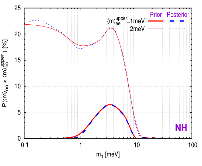
Figure 1: The probability of $\langle m\rangle_{ee}<1\,\mbox{meV}$ (thick) and $\langle m\rangle_{ee}<2\,\mbox{meV}$ (thin) for NH and given value of $m_{1}$, before (prior as solid lines) and after (posterior as dashed lines) JUNO/RENO-50 experiments.

In Fig. 1, we show the probability of $\langle m\rangle_{ee}$ being below $1\,\mbox{meV}$ and $2\,\mbox{meV}$ for NH, as a function of $m_{1}$. For $1\,\mbox{meV}\lesssim m_{1}\lesssim 10\,\mbox{meV}$, the effective mass $\langle m\rangle_{ee}$ has as large as $7\%$ of chance to be smaller than $1\,\mbox{meV}$ [39]. Above $\langle m\rangle_{ee}^{upper}=1\,\mbox{meV}$, the chance increases very fast. For $\langle m\rangle_{ee}^{upper}=2\,\mbox{meV}$, the chance jumps to around 20% once $m_{1}$ goes below $10\,\mbox{meV}$. We show the results before and after JUNO/RENO-50 as solid and dashed lines for comparison. Although the precision measurement of the solar angle $\theta_{s}$ has significant effect on the lower limit of $\langle m\rangle_{ee}$ for both NH and IH [48], its effect on the probability $P(\langle m\rangle_{ee}<\langle m\rangle_{ee}^{upper})$ is not that significant after marginalization.

Recently, the cosmological data provide the most stringent constraint on the scale of neutrino masses [37] preferring slightly NH. Since the two mass squares $\Delta m^{2}_{a}$ and $\Delta m^{2}_{s}$ have been measured, the cosmological data can also constrain the lightest mass $m_{1}$ [40].

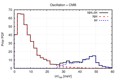
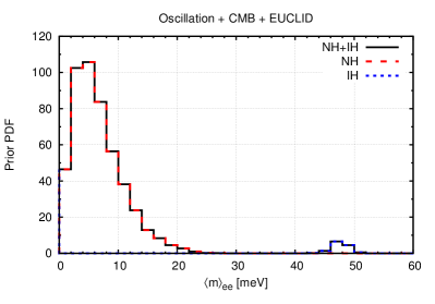
Figure 2: The probability distribution function (PDF) of the $0\nu 2\beta$ decay effective mass $\langle m\rangle_{ee}$, sampled from the global fit [44] of the neutrino oscillation parameters (oscillation), and the constraint on $m_{1}$ from the Planck data (CMB) plus the prospective data from EUCLID-like survey (EUCLID) [40]. Both NH (long-dashed red line) and IH (short-dashed blue line) have been sampled. The combined effect of NH and IH is shown as solid black line.

In Fig. 2, we show the sampled distribution of $\langle m\rangle_{ee}$ from both neutrino oscillation measurements [44] and cosmological constraint [40]. The cosmological data predicts the probability for NH versus IH to be around 2:1. This appears in the left panel of Fig. 2 as a larger peak around $\langle m\rangle_{ee}\approx 5\,\mbox{meV}$ for NH while a smaller peak around $\langle m\rangle_{ee}\approx 50\,\mbox{meV}$ for IH. It can further increase to 12:1 if the prospective observation from a EUCLID-like survey is added. Then, the IH peak in the $\langle m\rangle_{ee}$ distribution in the right panel of Fig. 2 almost vanishes. The whole picture would not be affected much by precision measurement at future medium baseline reactor neutrino experiments JUNO/RENO-50.

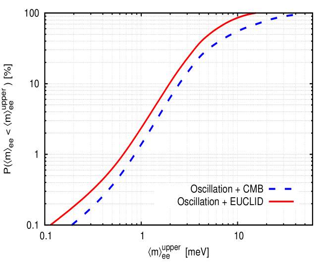
Figure 3: The predicted probability of $\langle m\rangle_{ee}<\langle m\rangle_{ee}^{upper}$ with neutrino oscillation measurements and Planck data (Oscillation + CMB) or the prospective observation from EUCLID-like survey (Oscillation + EUCLID), as a function of $\langle m\rangle_{ee}^{upper}$.

To show the picture more clearly, we plot the probability of $\langle m\rangle_{ee}<\langle m\rangle_{ee}^{upper}$ as a function of the upper value $\langle m\rangle_{ee}^{upper}$ in Fig. 3, after folding the cosmological data with the measurement of neutrino oscillation experiments. The curve starts from $P(\langle m\rangle_{ee}<0)=0\%$ to $100\%$ at large enough $\langle m\rangle_{ee}^{upper}\sim\mathcal{O}(10)\,\mbox{meV}$. Note that the global lower limit of $\langle m\rangle_{ee}$ for IH is around $13\,\mbox{meV}$ [48] and the chance for $\langle m\rangle_{ee}\lesssim 10\,\mbox{meV}$ is quite close to the naive estimation $67\%$ (92%) from the probability ratio $P(NH):P(IH)\approx 2:1$ (12:1). For more stringent constraints, $\langle m\rangle_{ee}$ has 1.3% (6%) of chance to be smaller than $1\,\mbox{meV}$ ($2\,\mbox{meV}$). It significantly increases to $2.2\%$ ($10\%$) if the EUCLID survey is available.

From the current constraints, the effective mass $\langle m\rangle_{ee}$ has a sizable chance to fall into the throat of the NH chimney which would imply a non-observation at current and up-coming $0\nu 2\beta$ decay experiments. Assuming that neutrinos are Majorana particles, we can then extract from the non-observation interesting results.

3 Extracting Majorana CP Phases from the Majorana Triangle

A non-observation of $0\nu 2\beta$ decay does not exclude the possibility of Majorana neutrinos. Since the $0\nu 2\beta$ signal is proportional to the $\langle m\rangle_{ee}$, it is possible that the Majorana CP phases $\delta_{\rm M1}$ and $\delta_{\rm M3}$ are such that there is no signal in the $ee$ channel. Reversely, non-observation can pin down $\delta_{\rm M1}$ and $\delta_{\rm M3}$ under the condition of neutrinos are Majorana particles.

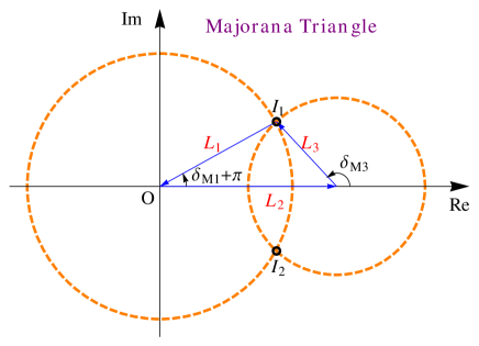
Figure 4: The Majorana Triangle in $0\nu 2\beta$ decay with vanishing $\langle m\rangle_{ee}$.

For illustration, we adopt the geometric plot [42] which is a variant of the Vissani graph [43]. In the complex plane, $\langle m\rangle_{ee}$ is a vector sum,

$$\langle m\rangle_{ee}\equiv\overrightarrow{L_{1}}+\overrightarrow{L_{2}}+\overrightarrow{L_{3}}\,,$$ (3.1)

as shown in Fig. 4. The three sides of the triangle are defined as,

$$\overrightarrow{L_{1}}\equiv m_{1}U^{2}_{e1}=m_{1}c^{2}_{r}c^{2}_{s}e^{i\delta_{\rm M1}}\,,$$ (3.2a)

$$\overrightarrow{L_{2}}\equiv m_{2}U^{2}_{e2}=\sqrt{m^{2}_{1}+\Delta m^{2}_{s}}c^{2}_{r}s^{2}_{s}\,,$$ (3.2b)

$$\overrightarrow{L_{3}}\equiv m_{3}U^{2}_{e3}=\sqrt{m^{2}_{1}+\Delta m^{2}_{a}}s^{2}_{r}e^{i\delta_{\rm M3}}\,.$$ (3.2c)

Correspondingly, the length of the three sides, $L_{1}=m_{1}c^{2}_{r}c^{2}_{s}$, $L_{2}=m_{2}c^{2}_{r}s^{2}_{s}$, and $L_{3}=m_{3}s^{2}_{r}$, is modulated by $m_{1}$, $m_{2}$, and $m_{3}$, respectively. In principle, there are three Majorana CP phases and only the two differences between them are physical. In the Vassani graph, $\delta_{\rm M1}$ is taken to be zero and $\overrightarrow{L_{1}}$ lies along the x-axis. This choice is convenient for vanishing $m_{1}$. Nevertheless, vanishing $\langle m\rangle_{ee}$ can only happen for nonzero $m_{1}$ with normal hierarchy. For this case, it is equivalent to take any one of three Majorana CP phases to be zero. With vanishing $\delta_{\rm M2}$, $\overrightarrow{L_{2}}$ lies along the x-axis while the other two vectors $\overrightarrow{L_{1}}$ and $\overrightarrow{L_{3}}$ rotate around the two ends of $\overrightarrow{L_{2}}$. Varying the two Majorana CP phases $\delta_{\rm M1}$ and $\delta_{\rm M3}$ , namely the direction of $\overrightarrow{L_{1}}$ and $\overrightarrow{L_{3}}$, draws two circles on the complex plane. The effective mass $\langle m\rangle_{ee}$ is then the vector between two arbitrary points on the two circles, respectively.

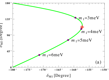
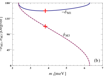
Figure 5: The predicted Majorana CP phases from vanishing $\langle m\rangle_{ee}$ with both (a) two-dimensional plot $\delta_{\rm M1}$–$\delta_{\rm M3}$ and (b) one-dimensional $\delta_{\rm M1}(m_{1})$/$\delta_{\rm M3}(m_{1})$ as implicit and explicit functions of the smallest mass $m_{1}$.

As shown in Fig. 4, the three sides ($\overrightarrow{L_{1}}$, $\overrightarrow{L_{2}}$, $\overrightarrow{L_{3}}$) can form a Majorana Triangle with vanishing $\langle m\rangle_{ee}$ if the two circles touch each other [42],

$$\left|L_{1}-L_{3}\right|\leq L_{2}\leq L_{1}+L_{3}\,.$$ (3.3)

It can happen at two intersection points, $I_{1}$ and $I_{2}$ as shown in Fig. 4. Different from quadrilateral, the sides and angles of a triangle has unique correlation with each other. From the length of the three sides, we can immediately solve the two Majorana CP phases ,

$$\cos\delta_{\rm M1} = -\frac{L^{2}_{1}+L^{2}_{2}-L^{2}_{3}}{2L_{1}L_{2}}=-\frac{m^{2}_{1}c^{4}_{r}c^{4}_{s}+m^{2}_{2}c^{4}_{r}s^{4}_{s}-m^{2}_{3}s^{4}_{r}}{2m_{1}m_{2}c^{4}_{r}c^{2}_{s}s^{2}_{s}}\,,$$ (3.4a)

$$\cos\delta_{\rm M3} = +\frac{L^{2}_{1}-L^{2}_{2}-L^{2}_{3}}{2L_{2}L_{3}}=+\frac{m^{2}_{1}c^{4}_{r}c^{4}_{s}-m^{2}_{2}c^{4}_{r}s^{4}_{s}-m^{2}_{3}s^{4}_{r}}{2m_{2}m_{3}c^{2}_{r}s^{2}_{r}s^{2}_{s}}\,.$$ (3.4b)

The length of the three sides ($L_{1}$, $L_{2}$, $L_{3}$) are functions of oscillation parameters ($\Delta m^{2}_{a}$, $\Delta m^{2}_{s}$, $\theta_{r}$, $\theta_{s}$) and the absolute mass scale $m_{1}$. Most of them can be measured by neutrino oscillation experiments while the mass scale $m_{1}$ remains a free parameter. With all oscillation parameters fixed, the vanishing $\langle m\rangle_{ee}$ would draw a line in the two-dimensional space of $\delta_{\rm M1}$ and $\delta_{\rm M3}$, as implicit functions of the mass scale $m_{1}$ shown in Fig. 5(a). For comparison, we also show the explicit functions of $\delta_{\rm M1}(m_{1})$ and $\delta_{\rm M3}(m_{1})$ in Fig. 5(b). The cosine functions (3.4) have two solutions, one in the upper complex plane and the other in the lower plane. Due to symmetry, both solutions can exist, but for simplicity, we show only one of them. Note that $\delta_{\rm M1}(m_{1})$ and $\delta_{\rm M3}(m_{1})$ always appear in opposite planes. To be consistent with the Fig. 4, we show the solution with $-180^{\circ}\leq\delta_{\rm M1}\leq 0^{\circ}$ and $0^{\circ}\leq\delta_{\rm M3}\leq 180^{\circ}$.

Across the interested region, (3.3) or equivalently $2.3\,\mbox{meV}\lesssim m_{1}\lesssim 6.3\,\mbox{meV}$, as will be elaborated in Sec. 5 and shown in Fig. 10, $L_{1}$ increases linearly with $m_{1}$ while $L_{3}$ almost remains the same. In addition, $L_{1}$ is always larger than $L_{3}$. Although $L_{1}$ is proportional to the smallest mass $m_{1}$ while $L_{3}$ is proportional to the much larger $m_{3}$, there is an extra suppression $s^{2}_{r}\approx 2.3\%$ associated with $m_{3}$. Consequently, the intersection points $I_{1}$ and $I_{2}$ are always on the right-hand side of the origin $O$, see Fig. 4. Further, the vector $\overrightarrow{L_{3}}$ can take any direction since $I_{1}$ and $I_{2}$ can take any point of the smaller circle. Correspondingly, the $\overrightarrow{L_{1}}$ circle in Fig. 4 expands with $m_{1}$, first approaches the $\overrightarrow{L_{3}}$ circle with almost constant radius from the left, crosses it when $L_{1}=L_{2}-L_{3}$, and finally swallows it when $L_{1}=L_{2}+L_{3}$. In this process, $\delta_{\rm M3}(m_{1})$ decreases from $180^{\circ}$ to $0^{\circ}$. On the other hand, $\delta_{\rm M1}(m_{1})$ first increases from $-180^{\circ}$ to its maximal value when the three sides form a right triangle, $L^{2}_{2}=L^{2}_{1}+L^{2}_{3}$, and then decreases back to $-180^{\circ}$. The turning point happens around,

$$m^{2}_{1}=\frac{c^{4}_{r}s^{4}_{s}\Delta m^{2}_{s}-s^{4}_{r}\Delta m^{2}_{a}}{c^{4}_{r}(c^{2}_{s}-s^{2}_{s})+s^{4}_{r}}\approx\frac{s^{4}_{s}}{c^{2}_{s}-s^{2}_{s}}\Delta m^{2}_{s}\,.$$ (3.5)

Since $s^{2}_{r}\sim\mathcal{O}(\Delta m^{2}_{s}/\Delta m^{2}_{a})$, the numerator is dominated by $c^{4}_{r}s^{4}_{s}\Delta m^{2}_{s}$ while the denominator mainly comes from $c^{4}_{r}(c^{2}_{s}-s^{2}_{s})$. Note that the omitted contributions are introduced by $L_{3}$. The turning point roughly corresponds to $L_{1}=L_{2}$ and is dictated by the solar parameters $\theta_{s}$ and $\Delta m^{2}_{s}$. Taking the current best fit values, the turning point happens around $m_{1}=4.3\,\mbox{meV}$ with $\delta_{\rm M1}=-158^{\circ}$ and $\delta_{\rm M3}=112^{\circ}$. To make it explicit, the turning point has been shown in Fig. 5 as red crosses. Although (3.5) is based on the observation that $L_{1}>L_{3}$ and $L_{3}$ remains approximately constant, it approximates the turning points very precisely. Since the three sides form a right triangle, the two Majorana CP phases are correlated with each other, $\delta_{\rm M3}=270^{\circ}+\delta_{\rm M1}$, at the turning point.

4 Uncertainties and Improvement from Reactor Neutrino Experiments

Considering the fact that the oscillation parameters ($\Delta m^{2}_{a}$, $\Delta m^{2}_{s}$, $\theta_{r}$, $\theta_{s}$) are not exactly measured, the prediction of $\delta_{\rm M1}$ and $\delta_{\rm M3}$ from the Majorana Triangle would become a band, instead of the single line in Fig. 5 (a).

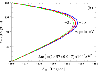
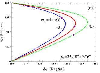
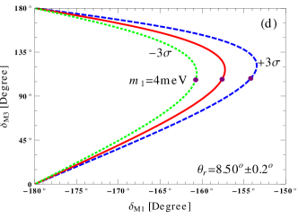
Figure 6: The contamination from the $3\sigma$ uncertainty [44] of oscillation parameters $\Delta m^{2}_{s}$, $\Delta m^{2}_{a}$, $\theta_{r}$, and $\theta_{s}$, respectively.

We show in Fig. 6 the $3\sigma$ variation of the predicted $\delta_{\rm M1}(m_{1})$ and $\delta_{\rm M3}(m_{1})$ on the four input oscillation parameters ($\Delta m^{2}_{a}$, $\Delta m^{2}_{s}$, $\theta_{r}$, $\theta_{s}$). The $\delta_{\rm M1}$–$\delta_{\rm M3}$ curve moves to the left when increasing the values of the solar parameter $\Delta m^{2}_{s}$ or $\theta_{s}$ and to the right for the atmospheric mass split $\Delta m^{2}_{a}$ or the reactor angle $\theta_{r}$. While $\Delta m^{2}_{a}$ and $\theta_{r}$ mainly affect $\delta_{\rm M1}$, the solar parameters mainly change $\delta_{\rm M3}$. Note that the x- and y-axes in Fig. 6 have quite different scale. The x-axis with plotted range $(-180^{\circ},-150^{\circ})$ is stretched by a factor of 6 than the y-axis which is plotted with the range $(0^{\circ},180^{\circ})$. Even with this magnification in the x-axis, the variation in $\delta_{\rm M3}$ when changing $\Delta m^{2}_{a}$ and $\theta_{r}$ is not visible. Although it becomes sizable when varying $\Delta m^{2}_{s}$ and $\theta_{s}$, the variation in $\delta_{\rm M1}$ is much smaller than in $\delta_{\rm M3}$. In addition, the variation from mass splits, $\Delta m^{2}_{s}$ and $\Delta m^{2}_{a}$, is relatively smaller than the one from mixing angles, $\theta_{s}$ and $\theta_{r}$. Precisely measuring the oscillation parameters ($\Delta m^{2}_{a}$, $\Delta m^{2}_{s}$, $\theta_{r}$, $\theta_{s}$), especially the two mixing angles, can help to determine the Majorana CP phases from vanishing $\langle m\rangle_{ee}$.

The same thing happens for the lower limit of $\langle m\rangle_{ee}$ [46]. For inverted hierarchy (IH), the effective mass $\langle m\rangle_{ee}$ cannot vanish. When varying the Majorana CP phases, $\langle m\rangle_{ee}$ spans a range. Its minimal value $\langle m\rangle_{ee}^{min}$ is a result of minimizing $\langle m\rangle_{ee}$ with respect to $\delta_{\rm M1}$ and $\delta_{\rm M3}$. Consequently, $\langle m\rangle_{ee}^{min}$ is also independent of $\delta_{\rm M1}$ and $\delta_{\rm M3}$, but a function of the smallest mass $m_{1}$ and the four oscillation parameters ($\Delta m^{2}_{a}$, $\Delta m^{2}_{s}$, $\theta_{r}$, $\theta_{s}$). Similarly, the largest uncertainty comes from the solar sector, especially $\theta_{s}$. With the global fit [47] at that time, the $3\sigma$ uncertainty in $\theta_{s}$ can introduce a factor of 6 difference in the required target mass for given sensitivity [48]. The only difference is that for IH, the two circles in Fig. 4 cannot touch each other since $L_{2}<L_{1}-L_{3}$. In this situation, the minimal value $\langle m\rangle_{ee}^{min}=L_{1}-L_{2}-L_{3}$ happens at $\delta_{\rm M1}=\pm 180^{\circ}$ and $\delta_{\rm M3}=0^{\circ}$. For NH, the minimal value $\langle m\rangle_{ee}^{min}$ can touch down to zero if (3.3) holds. Two conditions appear for the real and imaginary parts of $\langle m\rangle_{ee}^{min}$ to eliminate two degrees of freedom and produce the two equations in (3.4).

As pointed out in [48], both reactor neutrino oscillation and $0\nu 2\beta$ involve the same electron-electron channel. These two different phenomena share the same set of oscillation parameters ($\Delta m^{2}_{a}$, $\Delta m^{2}_{s}$, $\theta_{r}$, $\theta_{s}$). The measurement at reactor neutrino experiments can help to reduce the uncertainty in $0\nu 2\beta$ decay measurement. Since the reactor neutrino oscillation is well established by the observations at Daya Bay [49], RENO [51], and Double Chooz [52], the precision measurement of oscillation parameters there can help reduce the uncertainty in $0\nu 2\beta$ decay, especially when combining the measurements at both short and medium baseline reactor experiments. The short baseline (Daya Bay, RENO, Double Chooz) can measure the fast frequency oscillation due to $\Delta m^{2}_{a}$ and $\theta_{r}$ while the medium baseline (such as JUNO [54] and RENO-50 [55]) has better resolution on the slow frequency oscillation due to $\Delta m^{2}_{s}$ and $\theta_{s}$ [56]. Together, all of the four oscillation parameters ($\Delta m^{2}_{a}$, $\Delta m^{2}_{s}$, $\theta_{r}$, $\theta_{s}$) can be measured precisely. The advantage of reactor neutrino experiments is not just about measuring the smallest mixing angle $\theta_{r}$ and the neutrino mass hierarchy, but also significantly reducing the uncertainty in $0\nu 2\beta$ decay from oscillation parameters.

The effect of $\theta_{r}$ and $\theta_{s}$ uncertainties on $0\nu 2\beta$ decay can be found in [45] and [46]. With the reactor angle $\theta_{r}$ being precisely measured [50, 53], the major uncertainty now mainly comes from the solar angle $\theta_{s}$ [46, 48]. The next-generation of reactor neutrino experiments with medium baseline, such as JUNO [54] and RENO-50 [55] experiments can have very precise measurement on $\theta_{s}$, with relative uncertainty down to $\sim 0.3\%$ [54, 56]. The combination of Daya Bay and JUNO, one short baseline and the other medium baseline, can measure the four oscillation parameters $\Delta m^{2}_{s}$, $\Delta m^{2}_{a}$, $\theta_{r}$, and $\theta_{s}$ very precisely.

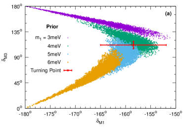
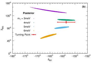
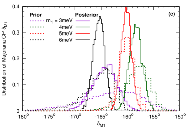
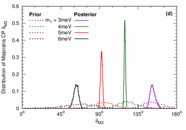
Figure 7: The prior (before JUNO) and posterior (after JUNO) distributions of the Majorana CP phases $\delta_{\rm M1}$ and $\delta_{\rm M3}$ determined from the Majorana Triangle with $m_{1}=3,4,5,6\,\mbox{meV}$, respectively. In the subplots we show (a) the prior 2-dimensional distribution $\delta_{\rm M1}$–$\delta_{\rm M3}$ with $\chi^{2}<9$, (b) the posterior 2-dimensional distribution $\delta_{\rm M1}$–$\delta_{\rm M3}$ with $\chi^{2}<9$, (c) the 1-dimensional distribution of $\delta_{\rm M1}$, and (d) the 1-dimensional distribution of $\delta_{\rm M3}$. The red crosses in (a) and (b) indicate the $3\sigma$ uncertainties in the values of $\delta_{\rm M1}$ and $\delta_{\rm M3}$ at turning points.

We use NuPro [57] to simulate JUNO for illustration and generate scattered points in the four-dimensional parameter space ($\Delta m^{2}_{a}$, $\Delta m^{2}_{s}$, $\theta_{r}$, $\theta_{s}$) with help of the Bayesian Nested Sampling algorithm [58] implemented in MultiNest [59]. Given a specific value of $m_{1}$, we obtain the distribution of predicted Majorana CP phases $\delta_{\rm M1}$ and $\delta_{\rm M3}$ according to (3.4). The Fig. 7 shows the results as both two-dimensional scattered plots with $\chi^{2}<9$ and one-dimensional histograms for the whole parameter space. As an illustration, we take four typical values $m_{1}=3,4,5,6\,\mbox{meV}$ within the considered range (3.3), or equivalently $2.3\,\mbox{meV}\lesssim m_{1}\lesssim 6.3\,\mbox{meV}$. With the current global fit [44] as prior constraints, the scattered points for $m_{1}=3,4,5,6\,\mbox{meV}$ overlap with each other in Fig. 7 (a). In comparison, the posterior distributions in Fig. 7 (b) after including JUNO are well separated from each other. Especially, the predictions for $m_{1}=3\,\mbox{meV}$ and $m_{1}=6\,\mbox{meV}$ no longer connects with the trivial solutions $\delta_{\rm M1}=-180^{\circ}$. Of the two Majorana CP phases $\delta_{\rm M1}$ and $\delta_{\rm M3}$, whose marginalized probability distributions are shown in Fig. 7 (c) and Fig. 7 (d), we observe more significant reduction in the uncertainty in $\delta_{\rm M3}$ than in $\delta_{\rm M1}$. This feature is consistent with the earlier observations that the uncertainty in $\theta_{s}$ has larger effect in $\delta_{\rm M3}$ than in $\delta_{\rm M1}$ and JUNO can mainly reduce the uncertainty of the solar parameters.

$1\sigma$ Uncertainties		Prior		Posterior
		$\delta_{\rm M1}$	$\delta_{\rm M3}$	$\delta_{\rm M1}$	$\delta_{\rm M3}$
$m_{1}=$	$3\,\mbox{meV}$	$-164^{\circ}\pm 5.4^{\circ}$	$149^{\circ}\pm 10.8^{\circ}$	$-165^{\circ}\pm 2.4^{\circ}$	$152^{\circ}\pm 3.3^{\circ}$
	$4\,\mbox{meV}$	$-159^{\circ}\pm 2.6^{\circ}$	$120^{\circ}\pm 10.8^{\circ}$	$-158^{\circ}\pm 1.2^{\circ}$	$120^{\circ}\pm 0.8^{\circ}$
	$5\,\mbox{meV}$	$-161^{\circ}\pm 1.5^{\circ}$	$91.7^{\circ}\pm 12.5^{\circ}$	$-160^{\circ}\pm 1.0^{\circ}$	$92.2^{\circ}\pm 1.2^{\circ}$
	$6\,\mbox{meV}$	$-166^{\circ}\pm 3.1^{\circ}$	$61.7^{\circ}\pm 17.1^{\circ}$	$-166^{\circ}\pm 1.1^{\circ}$	$62.4^{\circ}\pm 2.9^{\circ}$
Turning Point		$m_{1}=(4.31\pm 0.46)\,\mbox{meV}$		$m_{1}=(4.29\pm 0.05)\,\mbox{meV}$
		$-158^{\circ}\pm 2.2^{\circ}$	$112^{\circ}\pm 2.2^{\circ}$	$-159^{\circ}\pm 1.2^{\circ}$	$112^{\circ}\pm 1.2^{\circ}$

Table 1: The $1\sigma$ uncertainties of the two Majorana CP phases $\delta_{\rm M1}$ and $\delta_{\rm M3}$, the turning point parameters ($m_{1}$, $\delta_{\rm M1}$, $\delta_{\rm M3}$), and the upper limits $\langle m\rangle_{ee}^{upper}$ in (5.1) before and after JUNO/RENO-50.

Since the scales of $\delta_{\rm M1}$ and $\delta_{\rm M3}$ as shown in Fig. 7 are not the same, we list their $1\sigma$ uncertainties in Tab. 1. The uncertainty of $\delta_{\rm M1}$ is reduced by a factor of around $1.5\sim 3$ while $\delta_{\rm M3}$ by a factor of $3\sim 10$. This reflects the fact that the reduced uncertainty depends mostly on the solar parameters $\Delta m^{2}_{s}$ and $\theta_{s}$. The position uncertainty of the turning point even reduces by a factor of $10$, from $0.46\,\mbox{meV}$ to $0.05\,\mbox{meV}$. On the other hand, the uncertainties in the value $\delta_{\rm M1}$ and $\delta_{\rm M2}$ at the turning point reduce by only a factor of 2. Note that $\delta_{\rm M1}$ and $\delta_{\rm M2}$ have the same uncertainty, since they are correlated with each other, $\delta_{\rm M3}=270^{\circ}+\delta_{\rm M1}$, at the turning point. Altogether, given the smallest mass $m_{1}$, the Majorana Triangle with vanishing $\langle m\rangle_{ee}$ can predict the Majorana CP phases to degree level with the help of medium baseline reactor neutrino experiment such as JUNO or RENO-50. At that time, the largest uncertainty would almost entirely come from the unknown mass scale $m_{1}$ [60] and $0\nu 2\beta$ decay determination on $\langle m\rangle_{ee}$.

5 Sensitivity to Majorana CP Phases

As demonstrated in Sec. 3, from a non-observation of $0\nu 2\beta$ decay we can still infer the Majorana CP phases $\delta_{\rm M1}$ and $\delta_{\rm M3}$. In practice, non-observation can not lead to a exactly vanishing $\langle m\rangle_{ee}$, but an upper limit on it. The inferred $\delta_{\rm M1}$ and $\delta_{\rm M3}$ from the Majorana Triangle inevitably have uncertainty from the $0\nu 2\beta$ decay measurement, even with precision measurement of the oscillation parameters by reactor experiments. If the upper limit on $\langle m\rangle_{ee}$ is too large, the possible solution of Majorana CP phases can scan the whole region from the intersection $I_{1}$ to $I_{2}$ shown in Fig. 4. In other words, the Majorana CP phases can cross the trivial values $0^{\circ}$ or $\pm 180^{\circ}$. Requiring non-trivial solutions of the two Majorana CP phases, would place an upper limit on the uncertainty of $\langle m\rangle_{ee}$ and hence requirement on the design of future $0\nu 2\beta$ experiments.

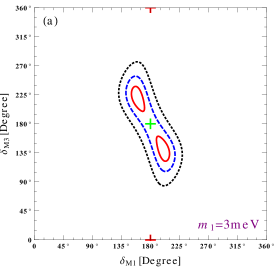
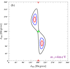
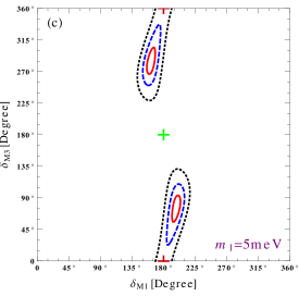
Figure 8: The contour plot of $\langle m\rangle_{ee}$ in the $\delta_{\rm M1}$–$\delta_{\rm M3}$ space with the lightest mass eigenvalues $m_{1}=(3,4,5,6)\,\mbox{meV}$ for the 4 panels and upper limits on $\langle m\rangle_{ee}=(0.3,0.6,1)\,\mbox{meV}$ depicted in ( solid, dashed, dotted) curves. In addition, the two trivial solutions ($\delta_{\rm M1}=\delta_{\rm M3}=180^{\circ}$) and ($\delta_{\rm M1}=180^{\circ}$, $\delta_{\rm M3}=0^{\circ},360^{\circ}$) appear as green and red crosses, respectively.

We show in Fig. 8 the $\langle m\rangle_{ee}$ contour on the $\delta_{\rm M1}$–$\delta_{\rm M3}$ plane for specific values of the smallest mass, $m_{1}=(3,4,5,6)\,\mbox{meV}$ in the four subplots. Each subplot shows three contours with $\langle m\rangle_{ee}=(0.3,0.6,1)\,\mbox{meV}$. Since we show the full range of $\delta_{\rm M1}$ and $\delta_{\rm M3}$ from $0^{\circ}$ to $360^{\circ}$, we can see two non-trivial solutions of vanishing $\langle m\rangle_{ee}$. The one in the lower-right quadrant, $180^{\circ}<\delta_{\rm M1}<360^{\circ}$ and $0^{\circ}<\delta_{\rm M3}<180^{\circ}$ corresponds to the solution shown in earlier plots while there is a symmetric solution in the upper-left quadrant. In addition, there are two trivial points of the Majorana CP phases, shown as green and red crosses in Fig. 8. The first, $\delta_{\rm M1}=\delta_{\rm M3}=180^{\circ}$, happens for $L_{2}-L_{3}<L_{1}<L_{2}$ while the second for $\delta_{\rm M1}=180^{\circ}$ and $\delta_{\rm M3}=0^{\circ}$. The contours around the two non-trivial solutions of vanishing $\langle m\rangle_{ee}$ would merge into a single contour if the trivial points $\delta_{\rm M1}=180^{\circ}$ and $\delta_{\rm M3}=0^{\circ}(360^{\circ})$ are also covered for larger value of $\langle m\rangle_{ee}$. Otherwise, the two solutions are isolated and non-trivial Majorana CP phases can be inferred.

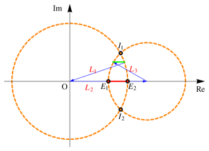
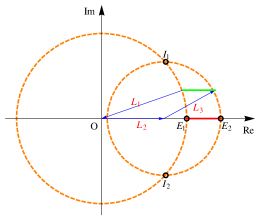
Figure 9: Geometrical illustration of the required sensitivity (red bar), or equivalently upper limit $\langle m\rangle_{ee}^{upper}$, to have non-trivial solutions of the Majorana CP phases if $0\nu 2\beta$ decay is not observed. The left plot is for $L_{1}<L_{2}$ while the right for $L_{1}>L_{2}$.

For illustration, we show the non-zero $\langle m\rangle_{ee}$ as a green bar in Fig. 9. Given the uncertainty $\Delta(\langle m\rangle_{ee})$, the green bar can slip around the intersection points $I_{1}$ or $I_{2}$, as long as $\langle m\rangle_{ee}\leq\Delta(\langle m\rangle_{ee})$. The largest value of $\langle m\rangle_{ee}$ between $I_{1}$ and $I_{2}$ is the distance between $E_{1}$ and $E_{2}$. If the green bar is longer than the red bar between $E_{1}$ and $E_{2}$, it can cross the x-axis and lead to trivial solutions, namely $\delta_{\rm M1}=\pm 180^{\circ}$ and $\delta_{\rm M3}=0^{\circ},180^{\circ}$ when it lies on the x-axis. To guarantee non-trivial Majorana CP phases, the sensitivity $\langle m\rangle_{ee}^{upper}$ cannot be larger than the length of the red bar,

$$\langle m\rangle_{ee}^{upper}<\begin{cases}L_{1}+L_{3}-L_{2}\qquad\mbox{for}\qquad L_{1}<L_{2}\,,\\ L_{2}+L_{3}-L_{1}\qquad\mbox{for}\qquad L_{1}>L_{2}\,.\end{cases}$$ (5.1)

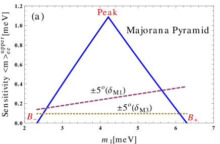
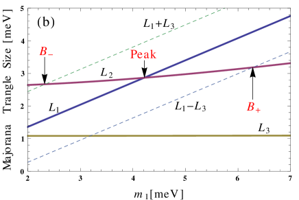
Figure 10: (a) The required sensitivity $\langle m\rangle_{ee}^{upper}$ on $\langle m\rangle_{ee}$ to guarantee non-trivial solutions of the Majorana CP phases, and (b) the corresponding boundary and peak points.

In Fig. 10 (a) we show the required sensitivity $\langle m\rangle_{ee}^{upper}$ to guarantee non-trivial Majorana CP phases as a function of the smallest mass $m_{1}$. Its shape resembles a pyramid, leading to a metaphor that the two Majorana CP phases $\delta_{\rm M1}$ and $\delta_{\rm M3}$ hiding in the Majorana Pyramid as snails lingering around as long as the sensitivity $\langle m\rangle_{ee}^{upper}$ is not low enough to touch them. The peak appears in the middle when $L_{1}=L_{2}$ with height being $L_{3}$,

$$\langle m\rangle_{ee}^{upper}\leq L_{3}=s^{2}_{r}\sqrt{\frac{s^{4}_{s}}{c^{2}_{s}-s^{2}_{s}}\Delta m^{2}_{s}+\Delta m^{2}_{a}}\approx s^{2}_{r}\sqrt{\Delta m^{2}_{a}}\approx 1.1\,\mbox{meV}\,.$$ (5.2)

It is interesting to see that the peak appears at $m^{peak}_{1}\equiv s^{2}_{s}\sqrt{\Delta m^{2}_{s}/(c^{2}_{s}-s^{2}_{s})}$ which is around the turning point (3.5). While the peak position is determined by the solar parameters $\Delta m^{2}_{s}$ and $\theta_{s}$, its height mainly is a function of the atmospheric mass split $\Delta m^{2}_{a}$ and the reactor angle $\theta_{r}$. From the top of the Majorana Pyramid, the sensitivity $\langle m\rangle_{ee}^{upper}$ decreases linearly with the deviation $m_{1}-m^{peak}_{1}$ from the peak position and vanishes at the two boundaries $B_{\pm}$ ($L_{1}-L_{2}=\pm L_{3}$) that corresponding to $m_{1}=2.3\,\mbox{meV}$ and $m_{1}=6.3\,\mbox{meV}$, respectively. Both peak and boundaries are functions of only the oscillation parameters ($\Delta m^{2}_{a}$, $\Delta m^{2}_{s}$, $\theta_{r}$, $\theta_{s}$) and are independent of any other unmeasured parameters. The Majorana Pyramid is well defined, especially after JUNO/RENO-50. To make the picture explicit, we show in Fig. 10 (b) the three sides ($L_{1}$, $L_{2}$, $L_{3}$) of the Majorana Triangle as functions of the smallest mass $m_{1}$ and indicate their relations with the peak and boundary positions. While the peak happens at the crossing point of $L_{1}$ and $L_{2}$, the boundaries $B_{\pm}$ happens at the crossing point of $L_{2}$ and $L_{1}\mp L_{3}$.

$\langle m\rangle_{ee}^{upper}$ (meV)	The smallest mass $m_{1}$
	3 meV	4 meV	5 meV	6 meV
Prior	$0.23\pm 0.18$	$0.75\pm 0.21$	$0.90\pm 0.18$	$0.48\pm 0.26$
Posterior	$0.21\pm 0.06$	$0.75\pm 0.06$	$0.97\pm 0.06$	$0.48\pm 0.06$

Table 2: The $1\sigma$ uncertainty of the required sensitivity $\langle m\rangle_{ee}^{upper}$ of the $0\nu 2\beta$ decay measurement for extracting non-trivial Majorana CP phases, before (Prior) and after (Posterior) JUNO/RENO-50.

The sensitivity $\langle m\rangle_{ee}^{upper}$ also suffers from the uncertainty in solar parameters. Although the largest value of $\langle m\rangle_{ee}^{upper}$ on the top of the Majorana Pyramid is mainly a function of the atmospheric mass split $\Delta m^{2}_{a}$ and the reactor angle $\theta_{r}$, see (5.2), the solar parameters $\Delta m^{2}_{s}$ and $\theta_{s}$ can still affect the sensitivity. This is especially true for the parameter space off the peak. We list the uncertainty of $\langle m\rangle_{ee}^{upper}$ for typical values $m_{1}=3,4,5,6\,\mbox{meV}$ in Tab. 2. The uncertainty for $m_{1}=3,6\,\mbox{meV}$ is relatively larger than for $m_{1}=4,5\,\mbox{meV}$. Without medium baseline reactor experiment JUNO/RENO-50, the $3\sigma$ uncertainty at the peak can be as large as roughly $100\%$. This can lead to a factor of $16$ difference in the required target mass for given sensitivity [46]. The JUNO/RENO-50 experiment can help to reduce this uncertainty by a factor of $3.5$. Correspondingly, the uncertainty in the required target mass reduces to around a factor of $2$. To guarantee the same sensitivity, the detector size can be reduced by a factor of 8 when designing future $0\nu 2\beta$ decay experiments.

In Fig. 10 we also show how a changing $\delta_{\rm M1}$ or $\delta_{\rm M3}$ alone can affect the effective mass $\langle m\rangle_{ee}$ for comparison. Around the vanishing $\langle m\rangle_{ee}$ we perturb the Majorana CP phases by $5$ degrees and plot the value of non-zero $\langle m\rangle_{ee}$ as a function of the smallest mass $m_{1}$. In other words, when the sensitivity on $\langle m\rangle_{ee}$ can be further pushed to these two lines, we can not only infer non-trivial values of $\delta_{\rm M1}$ and $\delta_{\rm M3}$, but constrain them with an uncertainty of only $5$ degrees. Different from the sensitivity curve as Majorana Pyramid, the $\pm 5^{\circ}$ curves do not change much across the range of $2.3\,\mbox{meV}\leq m_{1}\leq 6.3\,\mbox{meV}$. They are much lower than the peak value of $1.1\,\mbox{meV}$ and lies in the range $(0.1\sim 0.4)\,\mbox{meV}$. Pinning down the value of $\delta_{\rm M1}$ and $\delta_{\rm M3}$ is much harder than excluding trivial values, as expected.

6 Conclusions

In this paper we explore what a non-observation of $0\nu 2\beta$ decay can teach us if we assume that neutrinos are still Majorana particles. Although the absence of $0\nu 2\beta$ decay signal cannot verify the Majorana nature of neutrinos, it provides the possibility of uniquely fixing the two Majorana CP phases simultaneously from the Majorana Triangle with vanishing $\langle m\rangle_{ee}$. From the perspective of constraining model building, this situation would be even better than measuring a nonzero $\langle m\rangle_{ee}$ which can fix only one degree of freedom as a combination of the two Majorana CP phases. In addition, the smallest mass eigenvalue is limited to a narrow window, $2.3\,\mbox{meV}\lesssim m_{1}\lesssim 6.3\,\mbox{meV}$. The medium baseline reactor neutrino experiment JUNO/RENO-50 can help to significantly reduce the uncertainty in the predicted Majorana CP phases. In addition, the uncertainty in the required sensitivity for inferring non-trivial Majorana CP phases can also be reduced by the precision measurement of solar parameters $\Delta m^{2}_{s}$ and $\theta_{s}$ at JUNO/RENO-50.

To guarantee the ability of identifying non-trivial Majorana CP phases, the $0\nu 2\beta$ decay experiment needs to touch the Majorana Pyramid with impressive sensitivity $\langle m\rangle_{ee}^{upper}\lesssim 1.1\,\mbox{meV}$. This sensitivity is roughly $10$ times smaller than the ability of the next-generation $0\nu 2\beta$ decay experiments which can touch down to around $10\,\mbox{meV}$ and rough testify/falsify IH. Correspondingly, the detector scales with $\langle m\rangle_{ee}^{4}$ and needs to expand by a factor of $10^{4}$ which seems like a mission impossible. The situation may change if the background rate can be significantly suppressed below the signal rate. Then, the detector only needs to scale with $\langle m\rangle_{ee}^{2}$ and expand by a factor of $100$.

References

- [1] M. Zralek, “50 Years of Neutrino Physics,” Acta Phys. Polon. B 41, 2563 (2011) [arXiv:1012.2390 [hep-ph]]; S. M. Bilenky, “Neutrino. History of a unique particle,” Eur. Phys. J. H 38, 345 (2013) [arXiv:1210.3065 [hep-ph]]; J. Steinberger, “The history of neutrinos, 1930-1985. What have we learned about neutrinos? What have we learned using neutrinos?,” Annals Phys. 327, 3182 (2012) [Nucl. Phys. Proc. Suppl. 235-236, 485 (2013)]; S. M. Bilenky, “Neutrino oscillations: brief history and present status,” [arXiv:1408.2864 [hep-ph]].
- [2] S. L. Glashow, “Partial Symmetries of Weak Interactions,” Nucl. Phys. 22, 579 (1961); S. Weinberg, “A Model of Leptons,” Phys. Rev. Lett. 19, 1264 (1967); A. Salam, “Weak and Electromagnetic Interactions,” Conf. Proc. C 680519, 367 (1968).
- [3] B. Pontecorvo, “Mesonium and anti-mesonium,” Sov. Phys. JETP 6, 429 (1957) [Zh. Eksp. Teor. Fiz. 33, 549 (1957)]; Z. Maki, M. Nakagawa and S. Sakata, “Remarks on the unified model of elementary particles,” Prog. Theor. Phys. 28, 870 (1962).
- [4] J. N. Bahcall, “Solar neutrinos. I: Theoretical,” Phys. Rev. Lett. 12, 300 (1964); R. Davis, “Solar neutrinos. II: Experimental,” Phys. Rev. Lett. 12, 303 (1964); Q. R. Ahmad et al. [SNO Collaboration], “Direct evidence for neutrino flavor transformation from neutral current interactions in the Sudbury Neutrino Observatory,” Phys. Rev. Lett. 89, 011301 (2002) [arXiv:nucl-ex/0204008].
- [5] Y. Fukuda et al. [Super-Kamiokande Collaboration], “Evidence for oscillation of atmospheric neutrinos,” Phys. Rev. Lett. 81, 1562 (1998) [arXiv:hep-ex/9807003].
- [6] E. Majorana, “Theory of the Symmetry of Electrons and Positrons,” Nuovo Cim. 14, 171 (1937).
- [7] S. Willenbrock, “Symmetries of the standard model,” [arXiv:hep-ph/0410370].
- [8] M. Duerr, M. Lindner and A. Merle, “On the Quantitative Impact of the Schechter-Valle Theorem,” JHEP 1106, 091 (2011) [arXiv:1105.0901 [hep-ph]].
- [9] W. H. Furry, “On Transition Probabilities in Double Beta-Disintegration,” Phys. Rev. 56, 1184, (1939).
- [10] J. Schechter and J. W. F. Valle, “Neutrino Oscillation Thought Experiment,” Phys. Rev. D 23, 1666 (1981); L. F. Li and F. Wilczek, “Physical Processes Involving Majorana Neutrinos,” Phys. Rev. D 25, 143 (1982); J. Bernabeu and P. Pascual, “CP Properties of the Leptonic Sector for Majorana Neutrinos,” Nucl. Phys. B 228, 21 (1983); P. Langacker and J. Wang, “Neutrino anti-neutrino transitions,” Phys. Rev. D 58, 093004 (1998) [arXiv:hep-ph/9802383]; A. de Gouvea, B. Kayser and R. N. Mohapatra, “Manifest CP violation from Majorana phases,” Phys. Rev. D 67, 053004 (2003) [arXiv:hep-ph/0211394]; Z. Z. Xing, “Properties of CP Violation in Neutrino-Antineutrino Oscillations,” Phys. Rev. D 87, no. 5, 053019 (2013) [arXiv:1301.7654 [hep-ph]]; Z. Z. Xing and Y. L. Zhou, “Majorana CP-violating phases in neutrino-antineutrino oscillations and other lepton-number-violating processes,” Phys. Rev. D 88, 033002 (2013) [arXiv:1305.5718 [hep-ph]].
- [11] W. Rodejohann, “Inverse Neutrino-less Double Beta Decay Revisited: Neutrinos, Higgs Triplets and a Muon Collider,” Phys. Rev. D 81, 114001 (2010) [arXiv:1005.2854 [hep-ph]].
- [12] W. Rodejohann, “Neutrino-less Double Beta Decay and Particle Physics,” Int. J. Mod. Phys. E 20, 1833 (2011) [arXiv:1106.1334 [hep-ph]]; H. Pas and W. Rodejohann, “Neutrinoless Double Beta Decay,” New J. Phys. 17, no. 11, 115010 (2015) [arXiv:1507.00170 [hep-ph]].
- [13] J. Schechter and J. W. F. Valle, “Neutrinoless Double beta Decay in Theories,” Phys. Rev. D 25, 2951 (1982).
- [14] S. Dell’Oro, S. Marcocci, M. Viel and F. Vissani, “Neutrinoless double beta decay: 2015 review,” Adv. High Energy Phys. 2016, 2162659 (2016) [arXiv:1601.07512 [hep-ph]].
- [15] E. Andreotti et al., “130Te Neutrinoless Double-Beta Decay with CUORICINO,” Astropart. Phys. 34, 822 (2011) [arXiv:1012.3266 [nucl-ex]].
- [16] K. Alfonso et al. [CUORE Collaboration], “Search for Neutrinoless Double-Beta Decay of 130Te with CUORE-0,” Phys. Rev. Lett. 115, no. 10, 102502 (2015) [arXiv:1504.02454 [nucl-ex]].
- [17] D. R. Artusa et al. [CUORE Collaboration], “Searching for neutrinoless double-beta decay of 130Te with CUORE,” Adv. High Energy Phys. 2015, 879871 (2015) [arXiv:1402.6072 [physics.ins-det]].
- [18] S. Andringa et al. [SNO+ Collaboration], “Current Status and Future Prospects of the SNO+ Experiment,” Adv. High Energy Phys. 2016, 6194250 [arXiv:1508.05759 [physics.ins-det]].
- [19] H. V. Klapdor-Kleingrothaus et al., “Latest results from the Heidelberg-Moscow double beta decay experiment,” Eur. Phys. J. A 12, 147 (2001) [arXiv:hep-ph/0103062].
- [20] C. E. Aalseth et al. [IGEX Collaboration], “Neutrinoless double-beta decay of Ge-76: First results from the International Germanium Experiment (IGEX) with six isotopically enriched detectors,” Phys. Rev. C 59, 2108 (1999); C. E. Aalseth et al. [IGEX Collaboration], “The IGEX Ge-76 neutrinoless double beta decay experiment: Prospects for next generation experiments,” Phys. Rev. D 65, 092007 (2002) [arXiv:hep-ex/0202026].
- [21] K. H. Ackermann et al. [GERDA Collaboration], “The GERDA experiment for the search of decay in 76Ge,” Eur. Phys. J. C 73, no. 3, 2330 (2013) [arXiv:1212.4067 [physics.ins-det]]; M. Agostini et al. [GERDA Collaboration], “Results on Neutrinoless Double- Decay of 76Ge from Phase I of the GERDA Experiment,” Phys. Rev. Lett. 111, no. 12, 122503 (2013) [arXiv:1307.4720 [nucl-ex]].
- [22] R. Brugnera and A. Garfagnini, “Status of the GERDA Experiment at the Laboratori Nazionali del Gran Sasso,” Adv. High Energy Phys. 2013, 506186 (2013).
- [23] N. Abgrall et al. [Majorana Collaboration], “The Majorana Demonstrator Neutrinoless Double-Beta Decay Experiment,” Adv. High Energy Phys. 2014, 365432 (2014) [arXiv:1308.1633 [physics.ins-det]].
- [24] M. Agostini, Talk at Neutrino 2016 Conference, London, July 4-9, 2016, http://neutrino2016.iopconfs.org/IOP/media/uploaded/EVIOP/event_948/09.25__5__agostini.pdf.
- [25] J. B. Albert et al. [EXO-200 Collaboration], “Search for Majorana neutrinos with the first two years of EXO-200 data,” Nature 510, 229 (2014) [arXiv:1402.6956 [nucl-ex]].
- [26] A. Gando et al. [KamLAND-Zen Collaboration], “Search for Majorana Neutrinos near the Inverted Mass Hierarchy region with KamLAND-Zen,” [arXiv:1605.02889 [hep-ex]].
- [27] J. Mart n-Albo et al. [NEXT Collaboration], “Sensitivity of NEXT-100 to neutrinoless double beta decay,” JHEP 1605, 159 (2016) [arXiv:1511.09246 [physics.ins-det]].
- [28] A. Pocar [EXO-200 and nEXO Collaborations], “Searching for neutrino-less double beta decay with EXO-200 and nEXO,” Nucl. Part. Phys. Proc. 265-266, 42 (2015).
- [29] Xiangdong Ji, “PandaX and 0nDBD,” Presentation at the International Workshop on Baryon and Lepton Number Violation (BLV15), Amherst, MA, USA, April 2015.
- [30] R. Arnold et al. [NEMO-3 Collaboration], “Results of the search for neutrinoless double- decay in 100Mo with the NEMO-3 experiment,” Phys. Rev. D 92, no. 7, 072011 (2015) [arXiv:1506.05825 [hep-ex]].
- [31] V. Alenkov et al. [AMoRE Collaboration], “Technical Design Report for the AMoRE Decay Search Experiment,” [arXiv:1512.05957 [physics.ins-det]].
- [32] J. W. Beeman et al. [LUCIFER Collaboration], “Double-beta decay investigation with highly pure enriched 82Se for the LUCIFER experiment,” Eur. Phys. J. C 75, no. 12, 591 (2015) [arXiv:1508.01709 [physics.ins-det]].
- [33] R. Arnold et al. [SuperNEMO Collaboration], “Probing New Physics Models of Neutrinoless Double Beta Decay with SuperNEMO,” Eur. Phys. J. C 70, 927 (2010) [arXiv:1005.1241 [hep-ex]]; S. Blot [NEMO-3 and SuperNEMO experiments Collaborations], “Investigating decay with the NEMO-3 and SuperNEMO experiments,” J. Phys. Conf. Ser. 718, no. 6, 062006 (2016).
- [34] S. M. Bilenky, S. Pascoli and S. T. Petcov, “Majorana neutrinos, neutrino mass spectrum, CP violation and neutrinoless double beta decay. 1. The Three neutrino mixing case,” Phys. Rev. D 64, 053010 (2001) [arXiv:hep-ph/0102265].
- [35] W. Rodejohann, “Measuring leptonic CP violation in neutrinoless double beta decay,” [arXiv:hep-ph/0203214].
- [36] Z. Z. Xing, “Vanishing effective mass of the neutrinoless double beta decay?,” Phys. Rev. D 68, 053002 (2003) [arXiv:hep-ph/0305195].
- [37] S. Dell’Oro, S. Marcocci, M. Viel and F. Vissani, “The contribution of light Majorana neutrinos to neutrinoless double beta decay and cosmology,” JCAP 1512, no. 12, 023 (2015) [arXiv:1505.02722 [hep-ph]]; Q. G. Huang, K. Wang and S. Wang, “Constraints on the neutrino mass and mass hierarchy from cosmological observations,” [arXiv:1512.05899 [astro-ph.CO]]; E. Giusarma, M. Gerbino, O. Mena, S. Vagnozzi, S. Ho and K. Freese, “On the improvement of cosmological neutrino mass bounds,” [arXiv:1605.04320 [astro-ph.CO]].
- [38] F. Capozzi, E. Lisi, A. Marrone, D. Montanino and A. Palazzo, “Neutrino masses and mixings: Status of known and unknown parameters,” Nucl. Phys. B 908, 218 (2016) [arXiv:1601.07777 [hep-ph]].
- [39] G. Benato, “Effective Majorana Mass and Neutrinoless Double Beta Decay,” Eur. Phys. J. C 75, no. 11, 563 (2015) [arXiv:1510.01089 [hep-ph]].
- [40] S. Hannestad and T. Schwetz, “Cosmology and the neutrino mass ordering,” [arXiv:1606.04691 [astro-ph.CO]].
- [41] Z. Z. Xing, Z. H. Zhao and Y. L. Zhou, “How to interpret a discovery or null result of the decay,” Eur. Phys. J. C 75, no. 9, 423 (2015) [arXiv:1504.05820 [hep-ph]].
- [42] Z. Z. Xing and Y. L. Zhou, “Geometry of the effective Majorana neutrino mass in the decay,” Chin. Phys. C 39, 011001 (2015) [arXiv:1404.7001 [hep-ph]].
- [43] F. Vissani, “Signal of neutrinoless double beta decay, neutrino spectrum and oscillation scenarios,” JHEP 9906, 022 (1999) [arXiv:hep-ph/9906525].
- [44] M. C. Gonzalez-Garcia, M. Maltoni and T. Schwetz, “Global Analyses of Neutrino Oscillation Experiments,” [arXiv:1512.06856 [hep-ph]].
- [45] M. Lindner, A. Merle and W. Rodejohann, “Improved limit on theta(13) and implications for neutrino masses in neutrino-less double beta decay and cosmology,” Phys. Rev. D 73, 053005 (2006) [arXiv:hep-ph/0512143].
- [46] A. Dueck, W. Rodejohann and K. Zuber, “Neutrinoless Double Beta Decay, the Inverted Hierarchy and Precision Determination of ,” Phys. Rev. D 83, 113010 (2011) [arXiv:1103.4152 [hep-ph]].
- [47] D. V. Forero, M. Tortola and J. W. F. Valle, “Neutrino oscillations refitted,” Phys. Rev. D 90, no. 9, 093006 (2014) [arXiv:1405.7540 [hep-ph]].
- [48] S. F. Ge and W. Rodejohann, “JUNO and Neutrinoless Double Beta Decay,” Phys. Rev. D 92, no. 9, 093006 (2015) [arXiv:1507.05514 [hep-ph]].
- [49] F. P. An et al. [Daya Bay Collaboration], “Observation of electron-antineutrino disappearance at Daya Bay,” Phys. Rev. Lett. 108, 171803 (2012) [arXiv:1203.1669 [hep-ex]]; F. P. An et al. [Daya Bay Collaboration], “Measurement of the Reactor Antineutrino Flux and Spectrum at Daya Bay,” Phys. Rev. Lett. 116, no. 6, 061801 (2016) [arXiv:1508.04233 [hep-ex]]; F. P. An et al. [Daya Bay Collaboration], “New measurement of via neutron capture on hydrogen at Daya Bay,” Phys. Rev. D 93, no. 7, 072011 (2016) [arXiv:1603.03549 [hep-ex]].
- [50] J. Cao and K. B. Luk, “An overview of the Daya Bay Reactor Neutrino Experiment,” Nucl. Phys. B 908, 62 (2016) [arXiv:1605.01502 [hep-ex]].
- [51] J. K. Ahn et al. [RENO Collaboration], “Observation of Reactor Electron Antineutrino Disappearance in the RENO Experiment,” Phys. Rev. Lett. 108, 191802 (2012) [arXiv:1204.0626 [hep-ex]]; J. H. Choi et al. [RENO Collaboration], “Observation of Energy and Baseline Dependent Reactor Antineutrino Disappearance in the RENO Experiment,” Phys. Rev. Lett. 116, no. 21, 211801 (2016) [arXiv:1511.05849 [hep-ex]].
- [52] Y. Abe et al. [Double Chooz Collaboration], “Reactor electron antineutrino disappearance in the Double Chooz experiment,” Phys. Rev. D 86, 052008 (2012) [arXiv:1207.6632 [hep-ex]]; Y. Abe et al. [Double Chooz Collaboration], “First Measurement of from Delayed Neutron Capture on Hydrogen in the Double Chooz Experiment,” Phys. Lett. B 723, 66 (2013) [arXiv:1301.2948 [hep-ex]].
- [53] F. Suekane et al. [Double Chooz Collaboration], “Double Chooz and a history of reactor experiments,” Nucl. Phys. B 908, 74 (2016) [arXiv:1601.08041 [hep-ex]].
- [54] F. An et al. [JUNO Collaboration], “Neutrino Physics with JUNO,” J. Phys. G 43, no. 3, 030401 (2016) [arXiv:1507.05613 [physics.ins-det]].
- [55] S. B. Kim, “New results from RENO and prospects with RENO-50,” Nucl. Part. Phys. Proc. 265-266, 93 (2015) [arXiv:1412.2199 [hep-ex]].
- [56] S. F. Ge, K. Hagiwara, N. Okamura and Y. Takaesu, “Determination of mass hierarchy with medium baseline reactor neutrino experiments,” JHEP 1305, 131 (2013) [arXiv:1210.8141 [hep-ph]].
- [57] S. F. Ge, “NuPro: a simulation package for neutrino properties”, http://nupro.hepforge.org.
- [58] J. Skilling, “Nested sampling for general Bayesian computation,” Bayesian Analysis, 1(4):833-859, 12 2006.
- [59] F. Feroz, M. P. Hobson and M. Bridges, “MultiNest: an efficient and robust Bayesian inference tool for cosmology and particle physics,” Mon. Not. Roy. Astron. Soc. 398, 1601 (2009) [arXiv:0809.3437 [astro-ph]]; F. Feroz and M. P. Hobson, “Multimodal nested sampling: an efficient and robust alternative to MCMC methods for astronomical data analysis,” Mon. Not. Roy. Astron. Soc. 384, 449 (2008) [arXiv:0704.3704 [astro-ph]]; F. Feroz, M. P. Hobson, E. Cameron and A. N. Pettitt, “Importance Nested Sampling and the MultiNest Algorithm,” [arXiv:1306.2144 [astro-ph.IM]].
- [60] S. Maedan, “Predicted value of -decay effective Majorana mass with error of lightest neutrino mass,” [arXiv:1605.06871 [hep-ph]].