LU TP 16-44

August 2016

Pion light-by-light contributions to the muon $g-2$ Johan Bijnens and Johan Relefors
Department of Astronomy and Theoretical Physics, Lund University,

Sölvegatan 14A, SE 223-62 Lund, Sweden

This paper contains some new results on the hadronic light-by-light contribution (HLbL) to the muon $g-2$. The first part argues that we can expect large effects from disconnected diagrams in present and future calculations by lattice QCD of HLbL. The argument is based on the dominance of pseudo-scalar meson exchange.

In the second part, we revisit the pion loop HLbL contribution to the muon anomalous magnetic moment. We study it in the framework of some models studied earlier, pure pion loop, full VMD and hidden local symmetry for inclusion of vector mesons. In addition we study possible ways to include the axial-vector meson. The main part of the work is a detailed study of how the different momentum regions contribute. We derive a short distance constraint on the $\gamma^{*}\gamma^{*}\to\pi\pi$ amplitude and use this as a constraint on the models used for the pion loop. As a byproduct we present the general result for integration using the Gegenbauer polynomial method.

1 Introduction

The muon anomalous magnetic moment is one of the most precise measured quantities in high energy physics. The muon anomaly measures the deviation of the magnetic moment away from the prediction of a Dirac point particle

$$a_{\mu}\equiv\frac{g_{\mu}-2}{2}\,.$$ (1)

where $g_{\mu}$ is the gyromagnetic ratio $\vec{M}=g_{\mu}(e/2m_{\mu})\vec{S}$. The most recent experiment at BNL [1, 2, 3, 4] obtains the value

$$a_{\mu}=11\ 659\ 208.9(5.4)(3.3)~{}10^{-10}\,,$$ (2)

an impressive precision of 0.54 ppm (or 0.3 ppb on $g_{\mu}$). The new experiment at Fermilab aims to improve this precision to 0.14 ppm [5] and there is a discussion whether a precision of 0.01 ppm is feasible [6]. In order to fully exploit the reach of these experiments an equivalent precision needs to be reached by the theory. The theoretical prediction consist of three main parts, the pure QED contribution, the electroweak contribution and the hadronic contribution.

$$a_{\mu}=a_{\mu}^{\mathrm{QED}}+a_{\mu}^{\mathrm{EW}}+a_{\mu}^{\mathrm{had}}\,.$$ (3)

An introductory review of the theory is [7] and more comprehensive review are [8, 9]. Recent results can be found in the proceedings of the conferences [10, 11].

The hadronic part has two different contributions, those due to hadronic vacuum polarization, both at lowest and higher orders, and the light-by-light scattering contributions.

$$a_{\mu}^{\mathrm{had}}=a_{\mu}^{\mathrm{LO\mbox{-}HVP}}+a_{\mu}^{\mathrm{HO\mbox{-}HVP}}+a_{\mu}^{\mathrm{HLbL}}\,.$$ (4)

These are depicted symbolically in Fig. 1.

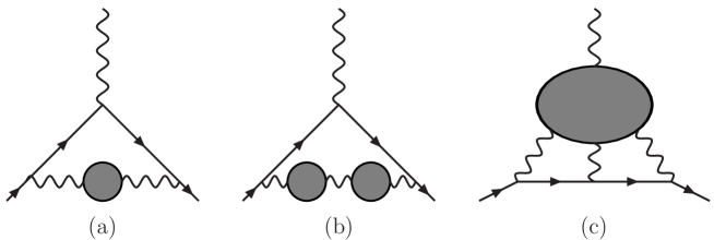
Figure 1: The thee main hadronic contributions to the muon anomalous magnetic moment. (a)The lowest order hadronic vacuum polarization. (b) An example of a higher order hadronic vacuum polarization contribution. (c) The light-by-light scattering contribution. In all three cases the shaded regions represent the hadronic part.

The hadronic vacuum polarization contributions can be related to the experimentally measured cross-section $e^{+}e^{-}\to$ hadrons. Here the accuracy can thus in principle be improved as needed for the experimental measurements of $a_{\mu}$.

The more difficult light-by-light contribution has no such simple relation to experimentally measurable quantities. A first comprehensive calculation appeared in [12]. One of the main problems there was the possibility of double counting when comparing quark-loop, hadron-loop and hadron exchange contributions. A significant step forward was done when it was realized [13] that the different contributions start entering at a different order in the expansion in the number of colours $N_{c}$ and in the chiral power counting, order in momentum $p$. This splitting was then used by two groups to estimate the light-by-light contribution [14, 15, 16](HKS) and [17, 18, 19](BPP). After correcting a sign mistake made by both groups for different reasons and discovered by [20] the results are

$$a_{\mu}^{\mathrm{HLbL}}=8.96(1.54)~{}10^{-10}~{}~{}(HKS),\qquad 8.3(3.2)~{}10^{-10}~{}~{}(BPP)\,.$$ (5)

A new developments since then have been the inclusion of short distance constraints on the full correction [21](MV) which indicated a larger contribution

$$a_{\mu}^{HLbL}=13.6(2.5)~{}10^{-10}~{}~{}(MV)\,.$$ (6)

Comparisons in detail of the various contributions in these three main estimates can be found in [22] and [23]. An indication of a possibly larger quark-loop contribution are the recent Schwinger-Dyson estimates of that contribution [24, 25, 26, 27]. First results of using dispersion relations to get an alternative handle on HLbL have also appeared [28, 29, 30, 31]. Lattice QCD has now started to contribute to HLbL as well, see e.g. [32, 33] and references therein.

In this paper we add a number of new results to the HLbL discussion. First, in Sect. 2 we present an argument why in the lattice calculations the disconnected contribution is expected to be large and of opposite sign to the connected contribution. This has been confirmed by the first lattice calculation [34]. The second part is extending the Gegenbauer polynomial method to do the integration over the photon momenta [20, 9] to the most general hadronic four-point function. This is the subject of Sect. 3. The third and largest part is about the charged pion and kaon loop. These have been estimated rather differently in the the three main evaluations

$$a_{\mu}^{\pi loop}=-0.45(0.81)~{}10^{-10}~{}(HKS),\quad-1.9(1.3)~{}10^{-10}~{}(BPP),\quad 0.0(1.0)~{}10^{-10}~{}(MV).$$ (7)

The numerical result is always dominated by the charged pion-loop, the charged kaon loop is about 5% of the numbers quoted in (7). The errors in all cases were mainly the model dependence. The main goal of this part is to show how these differences arise in the calculation and include a number of additional models. Given the uncertainties we will concentrate on the pion-loop only.

There are several improvements in this paper over the previous work on the pion loop. First, we use the Gegenbauer polynomial method of [9, 20] to do two more of the integrals analytically compared to the earlier work. Second, we study more models by including the vector mesons in a number of different ways and study the possible inclusion of axial-vector mesons. That the latter might introduce some uncertainty has been emphasized in [35, 36]. We present as well a new short-distance constraint that models have to satisfy for the underlying $\gamma\gamma\pi\pi$ vertex.

Our main tool for understanding the different results is to study the dependence on the virtualities of the three internal photons in Fig. 1(c). The use of this as a method to understand contributions was started in [22] for the main pion exchange. One aspect that will become clear is that one must be very careful in simply adding more terms in a hadronic model. In general, these models are non-renormalizable and there is thus no guarantee that there is a prediction for the muon anomaly in general. In fact, we have not found a clean way to do it for the axial vector meson as discussed in Sect. 4. However, using that the results should have a decent agreement with ChPT at low energies and the high-energy constraint and only integrating up to a reasonable hadronic scale we obtain the result

$$a_{\mu}^{HLbL~{}\pi loop}=-(2.0\pm 0.5)\cdot 10^{-10}\,.$$ (8)

This is discussed in Sect. 4.

A short summary is given in Sect. 5. Some of the results here have been presented earlier in [10, 37, 38] and [39].

2 Large disconnected contributions

Lattice calculations of HLbL are starting to give useful results. One question here is how to calculate the full contribution including both connected and disconnected contributions. The latter is more difficult to calculate, see e.g. [40], and many calculations so far have only presented results for the connected contribution. In this section we present an argument why the disconnected contribution is expected to be large and of opposite sign to the connected contribution. The connected contribution is the one where the four photons present in Fig. 1(c) all connect to the same quark line, the disconnected contribution where they connect to different quark lines. This is depicted schematically in Fig. 2.

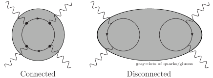
Figure 2: The connected contribution where all photons couple to a single quark-loop and an example of a disconnected diagram where the photons couple to different quark-loops.

The argument below is presented for the case of two-flavours and has been presented shortly in [38].

A large part of the HLbL contribution comes from pseudo-scalar meson exchange. For that part of the contribution we can give some arguments on the relative size of the disconnected and connected contribution. An example of a limit where the connected contribution is the only one is the large $N_{c}$ limit. One important consequence of this limit is that the anomalous breaking of the $U(1)_{A}$ symmetry disappears and the flavour singlet pseudo-scalar meson becomes light as well. This also applies to exchanges of other multiplets, but there the mass differences between the singlet and non-singlet states are much smaller.

Let us first look at the quark-loop case with two flavours. The connected diagram has four photon couplings, thus each quark flavour gives a contribution proportional to its charge to the power four. The connected contribution has thus a factor of $q_{u}^{4}+q_{d}^{4}=(2/3)^{4}+(-1/3)^{4}=17/81$. For the disconnected contribution we have instead charge factors of the form $(q_{u}^{2}+q_{d}^{2})$ for each quark-loop, so the final result has a factor of $(q_{u}^{2}+q_{d}^{2})^{2}=25/81$. However, this does not give any indication of the relative size since the contributions are very different.

In the large $N_{c}$ limit the mesons are the flavour eigenstates. We then have two light neutral pseudo-scalars, one with flavour content $\bar{u}u$, $\pi_{u}$ and one with $\bar{d}d$, $\pi_{d}$. In the meson exchange picture, shown in Fig. 3(a) the coupling of $\pi_{u}$ to two photons is proportional to $q_{u}^{2}$, thus $\pi_{u}$ exchange has factor of $q_{u}^{4}$. The same argument goes for the $\pi_{u}$ exchange and we obtain a factor of $q_{d}^{4}$. The total contribution is thus proportional to $q_{u}^{4}+q_{d}^{4}=17/81$ in agreement with the quark-loop argument for the same contribution.

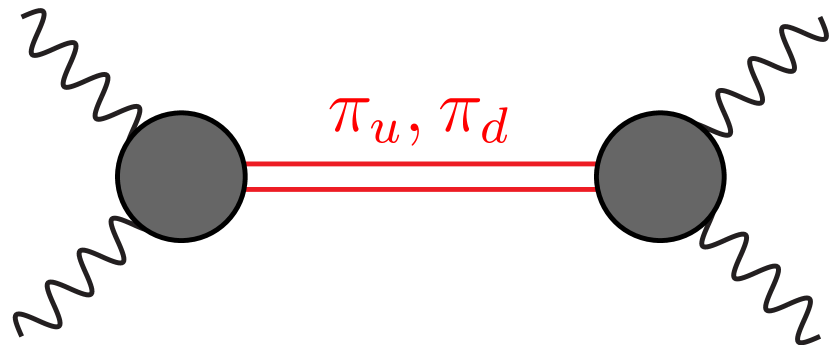
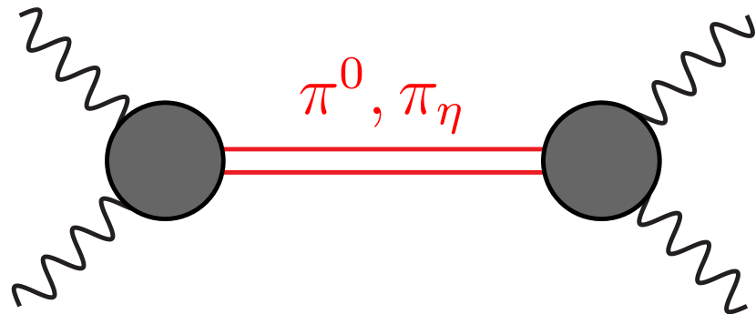
(a)           (b)

Figure 3: The meson-exchange picture. (a) With $\pi_{u}$ and $\pi_{d}$ exchange. (b) With $\pi^{0}$ and $\pi_{\eta}$ exchange.

We can also work with the isospin eigenstates instead. These are the $\pi^{0}$ with flavour content $(\bar{u}u-\bar{d}d)/\sqrt{2}$ and the flavour singlet $\pi_{\eta}$ with flavour content $(\bar{u}u+\bar{d}d)/\sqrt{2}$. In the large $N_{c}$ limit we should obtain the same result as with $\pi_{u}$ and $\pi_{d}$. The $\pi^{0}$ coupling to 2 photons is proportional to $\delta_{\pi^{0}}=(q_{u}^{2}-q_{d}^{2})/\sqrt{2}=3/(9\sqrt{2})$. The $\pi_{\eta}$ coupling to two photons is $\delta_{\pi_{\eta}}=(q_{u}^{2}+q_{d}^{2})/\sqrt{2}=5/(9\sqrt{2})$. The exchange of $\pi^{0}$ and $\pi_{\eta}$ leads to a contribution proportional to $\delta^{2}_{\pi^{0}}+\delta^{2}_{\pi_{\eta}}=17/81$ in agreement with the argument from the quark-loop or $\pi_{u},\pi_{d}$ exchange.

What happens now if we turn on the disconnected contribution or remove the large $N_{c}$ limit. The physical eigenstates are now $\pi_{\eta}$ and $\pi^{0}$ and they no longer have the same mass. In effect, from the breaking of the $U(1)_{A}$ the singlet has gotten a large mass and its contribution becomes much smaller. In the limit of being able to neglect $\pi_{\eta}$-exchange completely the sum of connected and disconnected contributions is reproduced by $\pi^{0}$ exchange alone which is proportional to $\delta_{\pi^{0}}^{2}=(9/2)/81$. So in this limit we expect the total contribution is $\delta_{\pi^{0}}^{2}$ times a factor $A$. From the discussion in the previous paragraph follows that the connected part is $\delta_{\pi^{0}}^{2}+\delta_{\pi_{\eta}}^{2}$ times the same factor $A$. The disconnected part must thus cancel the $\delta_{\pi}^{2}$ part of the connected contribution and must be $-\delta_{\pi_{\eta}}^{2}$ times again the factor $A$. We thus expect a large and negative disconnected contribution with a ratio of disconnected to connected of $-25/34$.

There are really three flavours $u,d,s$ to be considered but the argument generalizes straightforward to that case with case $\delta_{\pi^{0}}=3/(9\sqrt{2})$, $\delta_{\eta}=3/(9\sqrt{6})$ and $\delta_{\eta^{\prime}}=6/(9\sqrt{3})$. In the equal mass case the ratio of disconnected to connected is for three flavours $-\delta{\eta^{\prime}}^{2}/(\delta_{\pi^{0}}^{2}+\delta_{\eta}^{2}+\delta_{\eta^{\prime}}^{2})=-2/3$.

The above argument is valid in the equal mass limit, assuming the singlet does not contribute after $U(1)_{A}$ breaking is taken into account and only for the pseudo-scalar meson-exchange. There are corrections following from all of these. For most other contributions the disconnected effect is expected to be smaller. The ratio of disconnected to connected of $-2/3$ is thus an overestimate but given that $\pi^{0}$ exchange is the largest contribution we expect large and negative disconnected contributions.

Note that the above argument was in fact already used in the pseudo-scalar exchange estimate of [17, 18, 19], the comparison of the large $N_{c}$ estimate and $\pi^{0},\eta,\eta^{\prime}$ exchange is in Table 2 and the separate contributions in Table 3 of [18], up to the earlier mentioned overall sign.

Lattice QCD has been working hard on including disconnected contributions [40]. Using the same method of [32] at physical pion mass preliminary results were shown at Lattice 2016 [34] of $11.60(96)$ for the connected and $-6.25(80)$ for the disconnected in units of $10^{-10}$. This is in good agreement with the arguments given above.

3 The Gegenbauer polynomial method

The hadronic light-by-light contribution to the muon anomalous magnetic moment is given by [41]

$$a_{\mu}^{LbL}=\frac{-1}{48m_{\mu}}\mathrm{tr}\left[\left(p\hskip-4.2194pt/+m_{\mu}\right)M^{\lambda\beta}(0)\left(p\hskip-4.2194pt/+m_{\mu}\right)\left[\gamma_{\lambda},\gamma_{\beta}\right]\right]\,,$$ (9)

with

$$M^{\lambda\beta}(p_{3})=e^{6}\int\frac{d^{4}p_{1}}{(2\pi)^{4}}\frac{d^{4}p_{2}}{(2\pi)^{4}}\frac{\gamma_{\nu}\left(p_{4}\hskip-8.1805pt/\hskip 1.72218pt+m\right)\gamma_{\mu}\left(p_{5}\hskip-8.1805pt/\hskip 1.72218pt+m\right)\gamma_{\alpha}}{q^{2}p_{1}^{2}p_{2}^{2}\left(p_{4}^{2}-m^{2}\right)\left(p_{5}^{2}-m^{2}\right)}\left[\frac{\partial}{\partial p_{3\lambda}}\Pi^{\mu\nu\alpha\beta}\left(p_{1},p_{2},p_{3}\right)\right]\,.$$ (10)

Here $m$ is the muon mass, $p$ is the muon momentum, $q=p_{1}+p_{2}+p_{3}$, $p_{4}=p-p_{1}$ and $p_{5}=p+p_{2}$. The momentum routing in the diagram is shown in Fig. 4.

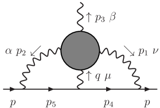
Figure 4: The momentum routing for the muon line and through the hadronic four-point function as used in (10).

Note that because of charge conjugation the integration in (10) is symmetric under the interchange of $p_{1}$ and $p_{2}$. The symmetry under the full interchange of $-q,p_{1},p_{2}$ is only explicitly present if the other permutations of the photons on the muon line are also added and then averaged. In this manuscript we stick to using only the permutation shown. The integral gives still the full contribution because the different permutations are included in the hadronic four-point function $\Pi^{\mu\nu\alpha\beta}(p_{1},p_{2},p_{3})$.

The hadronic four-point function is

$$\Pi^{\mu\nu\alpha\beta}(p_{1},p_{2},p_{3})=i^{3}\int d^{4}xd^{4}yd^{4}ze^{i(p_{1}\cdot x+p_{2}\cdot y+p_{3}\cdot z)}\langle 0|T\left(V^{\mu}(0)V^{\nu}(x)V^{\alpha}(y)V^{\beta}(z)\right)|0\rangle\,.$$ (11)

The current is $V_{\mu}=\sum_{q}Q_{q}\bar{q}\gamma_{\mu}q$ with $q$ denoting the quarks and $Q_{q}$ the quark charge in units of $|e|$. The four-point function has a rather complicated structure and we discuss this in more detail Sect. 3.1.

The partial derivative in (10) was introduced by [41] to make each photon leg permutation of the fermion-loop finite which allows to do the numerical calculation at $p_{3}=0$. It used $p_{3\beta}\Pi^{\mu\nu\alpha\beta}=0$ to obtain via $\partial/\partial p_{3\lambda}$

$$0=\Pi^{\mu\nu\alpha\lambda}+p_{3\beta}\frac{\partial}{\partial p_{3\lambda}}\Pi^{\mu\nu\alpha\beta}\,.$$ (12)

The integral in (10) contains 8 degrees of freedom. After projecting on the muon magnetic moment with (9) it can only depend on $p_{1}^{2},p_{2}^{2},p_{1}\cdot p_{2},p\cdot p_{1},p\cdot p_{2}$. The earlier work in [14, 15, 16, 17, 18, 19] relied on doing all these integrals numerically and in [17, 18, 19] this was done after an additional rotation to Euclidean space. For the pion exchange contribution a method was developed to reduce the number of integrals from 5 to 2 using the method of Gegenbauer polynomials [20]. The assumptions made there about the behaviour of the hadronic four-point function are not valid for the parts we study in this paper. However, in [9] for the pion and scalar exchange contributions the same method has been used to explicitly perform the integrals over the $p\cdot p_{1}$ and $p\cdot p_{2}$ degrees of freedom. The same method can be used to perform the integral over these two degrees of freedom also in the case for the most general four-point function. This leads to an expression of about 260 terms expressed in the combinations [18] of the four point function that contribute to the muon $g-2$. We have checked that our calculation reproduces for the pion exchange the results quoted in [9].

3.1 The general four-point function

The four-point functions defined in (11) contains 138 different Lorentz-structures [18]

$$\Pi^{\mu\nu\alpha\beta}(p_{1},p_{2},p_{3}) \equiv\Pi^{1}(p_{1},p_{2},p_{3})g^{\mu\nu}g^{\alpha\beta}+\Pi^{2}(p_{1},p_{2},p_{3})g^{\mu\alpha}g^{\nu\beta}$$

$$+\Pi^{3}(p_{1},p_{2},p_{3})g^{\mu\beta}g^{\nu\alpha}$$

$$+\Pi^{1jk}(p_{1},p_{2},p_{3})g^{\mu\nu}p_{j}^{\alpha}p_{k}^{\beta}+\Pi^{2jk}(p_{1},p_{2},p_{3})g^{\mu\alpha}p_{j}^{\nu}p_{k}^{\beta}$$

$$+\Pi^{3jk}(p_{1},p_{2},p_{3})g^{\mu\beta}p_{j}^{\nu}p_{k}^{\alpha}+\Pi^{4jk}(p_{1},p_{2},p_{3})g^{\nu\alpha}p_{j}^{\mu}p_{k}^{\beta}$$

$$+\Pi^{5jk}(p_{1},p_{2},p_{3})g^{\nu\beta}p_{j}^{\mu}p_{k}^{\alpha}+\Pi^{6jk}(p_{1},p_{2},p_{3})g^{\alpha\beta}p_{j}^{\mu}p_{k}^{\nu}$$

$$+\Pi^{ijkm}(p_{1},p_{2},p_{3})p_{i}^{\mu}p_{j}^{\nu}p_{k}^{\beta}p_{m}^{\alpha}\,,$$ (13)

where $i,j,k,m=$ 1, 2 or 3 and repeated indices are summed. The functions are scalar functions of all possible invariant products $p_{i}\cdot p_{j}$.

The four point function satisfies the Ward-Takahashi identities

$$q_{\mu}\Pi^{\mu\nu\alpha\beta}=p_{1\nu}\Pi^{\mu\nu\alpha\beta}=p_{2\alpha}\Pi^{\mu\nu\alpha\beta}=p_{3\beta}\Pi^{\mu\nu\alpha\beta}=0\,.$$ (14)

These identities allow to show that there are 43 independent functions in general. Of course, since the four-point function is symmetric under the interchange of the external legs many of these are related by permutations.

In practice it is easier not to do this reduction, but only the partial step up to reducing them to the 64 functions $\Pi^{ijkm}$. This can be done such that the powers of $p_{3}$ appearing explicitly never decrease. Not all of these contribute to $a_{\mu}$, in fact at most 32 combinations can contribute [18]. These are the $\Pi^{3jkm},\Pi^{i3km},\Pi^{ij3m}$ and the $\Pi^{Dijk}$, all with $i,j,k=1,2$. The $\Pi^{Dijk}$ come from derivatives of the $\Pi^{ijkm}$ w.r.t. $p_{3\lambda}$ at $p_{3}=0$

$$\frac{\partial}{\partial p_{3\lambda}}\Pi^{ijkm} =p_{1}^{\lambda}\Pi^{1ijkm}+p_{2}^{\lambda}\Pi^{2ijkm}$$

$$\Pi^{Dijk} =\Pi^{1ijk2}-\Pi^{2ijk1}\,.$$ (15)

3.2 The Gegenbauer method

The simplification introduced in [20] was that the Gegenbauer polynomial method can be used to average over all directions of the muon momentum. After this averaging is done there is only dependence on the invariant quantities $p_{1}^{2},p_{2}^{2}$ and $p_{1}\cdot p_{2}$ left. The method is fully explained in [9]. One can apply it to the full four-point function or to the one where one has reduced the number of components by using the Ward identities to the 64 $\Pi^{ijkl}$.

So we first take (9) and (10) and rotate everything to Euclidean momenta $P_{1}$, $P_{2}$ and $P$ with $Q=P_{1}+P_{2}$, $P_{4}=P-P_{1}$ and $P_{5}=P+P_{2}$. We see that the muon momentum $P$ shows up in denominators with $p_{4}^{2}-m^{2}=-(P_{4}^{2}+m^{2})$ and $p_{5}^{2}-m^{2}=-(P_{5}^{2}+m^{2})$ only. After taking the Dirac trace only scalar products of momenta are present in the numerator. Removing the products $P\cdot P_{1}$ and $P\cdot P_{2}$ by completing them to the full $P_{4}^{2}+m^{2}$ and $P_{5}^{2}+m^{2}$, the angular averaging over muon momenta can be performed using [9]

$$\left\langle\frac{1}{(P_{4}^{2}+m^{2})(P_{5}^{2}+m^{2})}\right\rangle_{\mu} = \delta X\,,$$

$$\left\langle\frac{P\cdot P_{1}}{P_{5}^{2}+m^{2}}\right\rangle_{\mu} = \frac{1}{8}\delta P_{1}\cdot P_{2}r_{2}^{2}\,,$$

$$\left\langle\frac{P\cdot P_{2}}{P_{4}^{2}+m^{2}}\right\rangle_{\mu} = \frac{1}{8}\delta P_{1}\cdot P_{2}r_{2}^{2}\,,$$

$$\left\langle\frac{1}{P_{4}^{2}+m^{2}}\right\rangle_{\mu} = \frac{1}{2}\delta r_{1}\,,$$

$$\left\langle\frac{1}{P_{5}^{2}+m^{2}}\right\rangle_{\mu} = \frac{1}{2}\delta r_{2}\,.$$ (16)

Here we used the notation

$$\delta = \frac{1}{m^{2}}\,,$$

$$r_{i} = 1-\sqrt{1+\frac{4m^{2}}{P_{i}^{2}}}$$

$$X = \frac{1}{P_{1}P_{2}\sin\theta}\mathrm{atan}\left(\frac{z\sin\theta}{1-z\cos\theta}\right)$$

$$\cos\theta = \frac{P_{1}\cdot P_{2}}{P_{1}P_{2}}$$

$$z = \frac{P_{1}P_{2}}{4m^{2}}r_{1}r_{2}\,.$$ (17)

The final contribution to the muon anomaly is given by

$$a_{\mu}=\frac{\alpha^{3}}{2\pi^{2}}\int P_{1}^{2}dP_{1}^{2}P_{2}^{2}dP_{2}^{2}\sin\theta d\cos\theta A_{\Pi}(P_{1},P_{2},\cos\theta)\,.$$ (18)

The quantity $A_{\Pi}$ is given by

$$\Pi^{1131} (-1/6\,\rho_{3}^{2}r_{2}^{2}\delta-2/3\,\rho_{1}\rho_{3}r_{2}\delta+8/3\,\rho_{1}\rho_{3}X-\,\rho_{1}^{2}r_{1}\delta-4/3\,\rho_{1}^{2}\rho_{3}X\delta-2\,\rho_{1}^{2}\rho_{2}X\delta)$$

$$+\Pi^{1132} (+2/3\rho_{3}+1/3\rho_{2}\rho_{3}r_{2}\delta-1/6\rho_{2}\rho_{3}r_{2}^{2}\delta-2/3\rho_{1}\rho_{3}r_{1}\delta-1/6\rho_{1}\rho_{3}r_{1}^{2}\delta-2/3\rho_{1}\rho_{2}r_{2}\delta$$

$$+1/3\rho_{1}\rho_{2}r_{1}\delta+8/3\rho_{1}\rho_{2}X-4/3\rho_{1}\rho_{2}\rho_{3}X\delta+2/3\rho_{1}\rho_{2}^{2}X\delta-4/3\rho_{1}^{2}\rho_{2}X\delta)$$

$$+\Pi^{1231} (-2/3\rho_{3}^{2}r_{2}\delta-1/6\rho_{2}\rho_{3}r_{2}^{2}\delta-2/3\rho_{1}\rho_{3}r_{1}\delta-4/3\rho_{1}\rho_{3}^{2}X\delta+1/3\rho_{1}\rho_{2}r_{2}\delta$$

$$+8/3\rho_{1}\rho_{2}X-4/3\rho_{1}\rho_{2}\rho_{3}X\delta+2/3\rho_{1}^{2}\rho_{2}X\delta)$$

$$+\Pi^{1232} (-2/3\rho_{3}^{2}r_{1}\delta-2/3\rho_{2}-2/3\rho_{2}\rho_{3}r_{2}\delta+8/3\rho_{2}\rho_{3}X-4/3\rho_{2}\rho_{3}^{2}X\delta-1/3\rho_{2}^{2}r_{2}\delta$$

$$-1/3\rho_{1}\rho_{2}r_{1}\delta-4/3\rho_{1}\rho_{2}\rho_{3}X\delta-2/3\rho_{1}\rho_{2}^{2}X\delta)$$

$$+\Pi^{1311} (+1/3\rho_{1}\rho_{3}r_{2}\delta+1/3\rho_{1}^{2}r_{1}\delta+2/3\rho_{1}^{2}\rho_{3}X\delta+2/3\rho_{1}^{2}\rho_{2}X\delta)$$

$$+\Pi^{1312} (-2/3\rho_{3}^{2}r_{2}\delta+4/3\rho_{3}^{2}X-1/12\rho_{2}\rho_{3}r_{2}^{2}\delta-4/3\rho_{1}\rho_{3}r_{1}\delta-1/12\rho_{1}\rho_{3}r_{1}^{2}\delta$$

$$-4/3\rho_{1}\rho_{3}^{2}X\delta+1/2\rho_{1}\rho_{2}r_{2}\delta+1/6\rho_{1}\rho_{2}r_{1}\delta+4/3\rho_{1}\rho_{2}X-8/3\rho_{1}\rho_{2}\rho_{3}X\delta$$

$$+1/3\rho_{1}\rho_{2}^{2}X\delta+\rho_{1}^{2}\rho_{2}X\delta)$$

$$+\Pi^{1322} (-2/3\rho_{2}-2/3\rho_{2}\rho_{3}r_{2}\delta+8/3\rho_{2}\rho_{3}X-1/3\rho_{2}^{2}r_{2}\delta-2\rho_{1}\rho_{2}r_{1}\delta$$

$$-4/3\rho_{1}\rho_{2}\rho_{3}X\delta-4\rho_{1}\rho_{2}^{2}X\delta)$$

$$+\Pi^{2131} (-2/3\rho_{1}-2/3\rho_{1}\rho_{3}r_{1}\delta+8/3\rho_{1}\rho_{3}X-2\rho_{1}\rho_{2}r_{2}\delta-4/3\rho_{1}\rho_{2}\rho_{3}X\delta-1/3\rho_{1}^{2}r_{1}\delta$$

$$-4\rho_{1}^{2}\rho_{2}X\delta)$$

$$+\Pi^{2231} (-2/3\rho_{3}^{2}r_{1}\delta+4/3\rho_{3}^{2}X-4/3\rho_{2}\rho_{3}r_{2}\delta-1/12\rho_{2}\rho_{3}r_{2}^{2}\delta-4/3\rho_{2}\rho_{3}^{2}X\delta-1/12\rho_{1}\rho_{3}r_{1}^{2}\delta$$

$$+1/6\rho_{1}\rho_{2}r_{2}\delta+1/2\rho_{1}\rho_{2}r_{1}\delta+4/3\rho_{1}\rho_{2}X-8/3\rho_{1}\rho_{2}\rho_{3}X\delta+\rho_{1}\rho_{2}^{2}X\delta+1/3\rho_{1}^{2}\rho_{2}X\delta)$$

$$+\Pi^{2232} (+1/3\rho_{2}\rho_{3}r_{1}\delta+1/3\rho_{2}^{2}r_{2}\delta+2/3\rho_{2}^{2}\rho_{3}X\delta+2/3\rho_{1}\rho_{2}^{2}X\delta)$$

$$+\Pi^{2311} (-2/3\rho_{3}^{2}r_{2}\delta-2/3\rho_{1}-2/3\rho_{1}\rho_{3}r_{1}\delta+8/3\rho_{1}\rho_{3}X-4/3\rho_{1}\rho_{3}^{2}X\delta-1/3\rho_{1}\rho_{2}r_{2}\delta$$

$$-4/3\rho_{1}\rho_{2}\rho_{3}X\delta-1/3\rho_{1}^{2}r_{1}\delta-2/3\rho_{1}^{2}\rho_{2}X\delta)$$

$$+\Pi^{2312} (-2/3\rho_{3}^{2}r_{1}\delta-2/3\rho_{2}\rho_{3}r_{2}\delta-4/3\rho_{2}\rho_{3}^{2}X\delta-1/6\rho_{1}\rho_{3}r_{1}^{2}\delta+1/3\rho_{1}\rho_{2}r_{1}\delta+8/3\rho_{1}\rho_{2}X$$

$$-4/3\rho_{1}\rho_{2}\rho_{3}X\delta+2/3\rho_{1}\rho_{2}^{2}X\delta)$$

$$+\Pi^{2321} (+2/3\rho_{3}-2/3\rho_{2}\rho_{3}r_{2}\delta-1/6\rho_{2}\rho_{3}r_{2}^{2}\delta+1/3\rho_{1}\rho_{3}r_{1}\delta-1/6\rho_{1}\rho_{3}r_{1}^{2}\delta+1/3\rho_{1}\rho_{2}r_{2}\delta$$

$$-2/3\rho_{1}\rho_{2}r_{1}\delta+8/3\rho_{1}\rho_{2}X-4/3\rho_{1}\rho_{2}\rho_{3}X\delta-4/3\rho_{1}\rho_{2}^{2}X\delta+2/3\rho_{1}^{2}\rho_{2}X\delta)$$

$$+\Pi^{2322} (-1/6\rho_{3}^{2}r_{1}^{2}\delta-2/3\rho_{2}\rho_{3}r_{1}\delta+8/3\rho_{2}\rho_{3}X-\rho_{2}^{2}r_{2}\delta-4/3\rho_{2}^{2}\rho_{3}X\delta-2\rho_{1}\rho_{2}^{2}X\delta)$$

$$+\Pi^{3111} (+1/6\rho_{3}^{2}r_{2}^{2}\delta-2/3\rho_{1}-4/3\rho_{1}\rho_{3}r_{2}\delta+1/2\rho_{1}\rho_{3}r_{2}^{2}\delta-1/3\rho_{1}\rho_{2}r_{2}\delta-\rho_{1}^{2}r_{2}\delta$$

$$-1/3\rho_{1}^{2}r_{1}\delta-8/3\rho_{1}^{2}\rho_{3}X\delta-2/3\rho_{1}^{2}\rho_{2}X\delta-2\rho_{1}^{3}X\delta)$$

$$+\Pi^{3112} (+4/3\rho_{3}+2/3\rho_{2}\rho_{3}r_{2}\delta+1/6\rho_{2}\rho_{3}r_{2}^{2}\delta+2/3\rho_{1}+2/3\rho_{1}\rho_{3}r_{1}\delta-1/3\rho_{1}\rho_{3}r_{1}^{2}\delta$$

$$-8/3\rho_{1}\rho_{3}X+2/3\rho_{1}\rho_{2}r_{1}\delta-8/3\rho_{1}\rho_{2}X+4/3\rho_{1}\rho_{2}\rho_{3}X\delta+4/3\rho_{1}\rho_{2}^{2}X\delta+1/3\rho_{1}^{2}r_{1}\delta)$$

$$+\Pi^{3121} (+2\rho_{1}+\rho_{1}^{2}r_{1}\delta)$$

$$+\Pi^{3122} (+2\rho_{2}+\rho_{2}^{2}r_{2}\delta)$$

$$+\Pi^{3211} (+4/3\rho_{3}-8/3\rho_{3}^{2}X+2/3\rho_{2}\rho_{3}r_{2}\delta+2/3\rho_{1}+2/3\rho_{1}\rho_{3}r_{1}\delta-1/6\rho_{1}\rho_{3}r_{1}^{2}\delta$$

$$-8/3\rho_{1}\rho_{3}X+1/3\rho_{1}\rho_{2}r_{2}\delta+1/3\rho_{1}\rho_{2}r_{1}\delta+4/3\rho_{1}\rho_{2}\rho_{3}X\delta+2/3\rho_{1}\rho_{2}^{2}X\delta$$

$$+1/3\rho_{1}^{2}r_{1}\delta+2/3\rho_{1}^{2}\rho_{2}X\delta)$$

$$+\Pi^{3212} (+4/3\rho_{3}-8/3\rho_{3}^{2}X+2/3\rho_{2}+2/3\rho_{2}\rho_{3}r_{2}\delta-1/6\rho_{2}\rho_{3}r_{2}^{2}\delta-8/3\rho_{2}\rho_{3}X$$

$$+1/3\rho_{2}^{2}r_{2}\delta+2/3\rho_{1}\rho_{3}r_{1}\delta+1/3\rho_{1}\rho_{2}r_{2}\delta+1/3\rho_{1}\rho_{2}r_{1}\delta+4/3\rho_{1}\rho_{2}\rho_{3}X\delta$$

$$+2/3\rho_{1}\rho_{2}^{2}X\delta+2/3\rho_{1}^{2}\rho_{2}X\delta)$$

$$+\Pi^{3221} (+4/3\rho_{3}+2/3\rho_{2}+2/3\rho_{2}\rho_{3}r_{2}\delta-1/3\rho_{2}\rho_{3}r_{2}^{2}\delta-8/3\rho_{2}\rho_{3}X+1/3\rho_{2}^{2}r_{2}\delta+2/3\rho_{1}\rho_{3}r_{1}\delta$$

$$+1/6\rho_{1}\rho_{3}r_{1}^{2}\delta+2/3\rho_{1}\rho_{2}r_{2}\delta-8/3\rho_{1}\rho_{2}X+4/3\rho_{1}\rho_{2}\rho_{3}X\delta+4/3\rho_{1}^{2}\rho_{2}X\delta)$$

$$+\Pi^{3222} (+1/6\rho_{3}^{2}r_{1}^{2}\delta-2/3\rho_{2}-4/3\rho_{2}\rho_{3}r_{1}\delta+1/2\rho_{2}\rho_{3}r_{1}^{2}\delta-1/3\rho_{2}^{2}r_{2}\delta-\rho_{2}^{2}r_{1}\delta-8/3\rho_{2}^{2}\rho_{3}X\delta$$

$$-2\rho_{2}^{3}X\delta-1/3\rho_{1}\rho_{2}r_{1}\delta-2/3\rho_{1}\rho_{2}^{2}X\delta)$$

$$+\Pi^{D111} (-1/3\rho_{1}\rho_{3}+2/3\rho_{1}\rho_{3}^{2}X-1/6\rho_{1}\rho_{2}\rho_{3}r_{2}\delta+1/24\rho_{1}\rho_{2}\rho_{3}r_{2}^{2}\delta-1/6\rho_{1}^{2}\rho_{3}r_{1}\delta$$

$$+1/24\rho_{1}^{2}\rho_{3}r_{1}^{2}\delta-1/12\rho_{1}^{2}\rho_{2}r_{2}\delta-1/12\rho_{1}^{2}\rho_{2}r_{1}\delta-2/3\rho_{1}^{2}\rho_{2}X-1/3\rho_{1}^{2}\rho_{2}\rho_{3}X\delta$$

$$-1/6\rho_{1}^{2}\rho_{2}^{2}X\delta-1/6\rho_{1}^{3}\rho_{2}X\delta)$$

$$+\Pi^{D121} (+1/3\rho_{3}^{2}-2/3\rho_{3}^{3}X+1/6\rho_{2}\rho_{3}^{2}r_{2}\delta-1/24\rho_{2}\rho_{3}^{2}r_{2}^{2}\delta+1/6\rho_{1}\rho_{3}^{2}r_{1}\delta-1/24\rho_{1}\rho_{3}^{2}r_{1}^{2}\delta$$

$$+1/12\rho_{1}\rho_{2}\rho_{3}r_{2}\delta+1/12\rho_{1}\rho_{2}\rho_{3}r_{1}\delta+2/3\rho_{1}\rho_{2}\rho_{3}X+1/3\rho_{1}\rho_{2}\rho_{3}^{2}X\delta+1/6\rho_{1}\rho_{2}^{2}\rho_{3}X\delta$$

$$+1/6\rho_{1}^{2}\rho_{2}\rho_{3}X\delta)$$

$$+\Pi^{D122} (+2/3\rho_{2}\rho_{3}-4/3\rho_{2}\rho_{3}^{2}X+1/3\rho_{2}^{2}\rho_{3}r_{2}\delta-1/12\rho_{2}^{2}\rho_{3}r_{2}^{2}\delta+1/3\rho_{1}\rho_{2}\rho_{3}r_{1}\delta$$

$$-1/12\rho_{1}\rho_{2}\rho_{3}r_{1}^{2}\delta+1/6\rho_{1}\rho_{2}^{2}r_{2}\delta+1/6\rho_{1}\rho_{2}^{2}r_{1}\delta+4/3\rho_{1}\rho_{2}^{2}X+2/3\rho_{1}\rho_{2}^{2}\rho_{3}X\delta$$

$$+1/3\rho_{1}\rho_{2}^{3}X\delta+1/3\rho_{1}^{2}\rho_{2}^{2}X\delta)$$

$$+\Pi^{D211} (-2/3\rho_{1}\rho_{3}+4/3\rho_{1}\rho_{3}^{2}X-1/3\rho_{1}\rho_{2}\rho_{3}r_{2}\delta$$

$$+1/12\rho_{1}\rho_{2}\rho_{3}r_{2}^{2}\delta-1/3\rho_{1}^{2}\rho_{3}r_{1}\delta+1/12\rho_{1}^{2}\rho_{3}r_{1}^{2}\delta-1/6\rho_{1}^{2}\rho_{2}r_{2}\delta-1/6\rho_{1}^{2}\rho_{2}r_{1}\delta$$

$$-4/3\rho_{1}^{2}\rho_{2}X-2/3\rho_{1}^{2}\rho_{2}\rho_{3}X\delta-1/3\rho_{1}^{2}\rho_{2}^{2}X\delta-1/3\rho_{1}^{3}\rho_{2}X\delta)$$

$$+\Pi^{D221} (-1/3\,\rho_{3}^{2}+2/3\,\rho_{3}^{3}X-1/6\,\rho_{2}\rho_{3}^{2}r_{2}\delta+1/24\,\rho_{2}\rho_{3}^{2}r_{2}^{2}\delta-1/6\,\rho_{1}\rho_{3}^{2}r_{1}\delta+1/24\,\rho_{1}\rho_{3}^{2}r_{1}^{2}\delta$$

$$-1/12\,\rho_{1}\rho_{2}\rho_{3}r_{2}\delta-1/12\,\rho_{1}\rho_{2}\rho_{3}r_{1}\delta-2/3\,\rho_{1}\rho_{2}\rho_{3}X-1/3\,\rho_{1}\rho_{2}\rho_{3}^{2}X\delta$$

$$-1/6\,\rho_{1}\rho_{2}^{2}\rho_{3}X\delta-1/6\,\rho_{1}^{2}\rho_{2}\rho_{3}X\delta)$$

$$+\Pi^{D222} (+1/3\,\rho_{2}\rho_{3}-2/3\,\rho_{2}\rho_{3}^{2}X+1/6\,\rho_{2}^{2}\rho_{3}r_{2}\delta-1/24\,\rho_{2}^{2}\rho_{3}r_{2}^{2}\delta+1/6\,\rho_{1}\rho_{2}\rho_{3}r_{1}\delta$$

$$-1/24\,\rho_{1}\rho_{2}\rho_{3}r_{1}^{2}\delta+1/12\,\rho_{1}\rho_{2}^{2}r_{2}\delta+1/12\,\rho_{1}\rho_{2}^{2}r_{1}\delta+2/3\,\rho_{1}\rho_{2}^{2}X+1/3\,\rho_{1}\rho_{2}^{2}\rho_{3}X\delta$$

$$+1/6\,\rho_{1}\rho_{2}^{3}X\delta+1/6\,\rho_{1}^{2}\rho_{2}^{2}X\delta)\,.$$ (19)

Here we used the abbreviations $\rho_{1}=P_{1}^{2}$, $\rho_{2}=P_{2}^{2}$ and $\rho_{3}=P_{1}\cdot P_{2}$. in addition to those defined above.

A more general formula without using the Ward identities can also be derived. Quoting this one would be too long. In practice for many models, the method without using Ward identities leads to shorter but equivalent results. We have used both options for the bare pion loop, the full VMD (Vector Meson Dominance) model and the hidden local symmetry (HLS) model and only the latter method for the antisymmetric field model for the vector and axial vector mesons.

4 The pion-loop contribution to HLbL

The pion loop contribution is depicted in Fig. 5. In the models we consider all the diagrams depicted can appear.

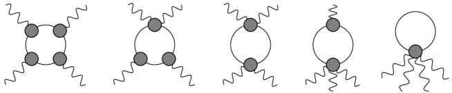
Figure 5: The pion-loop contributions to the vector four-point function of Eq. 11. The modeling is in the expressions for the form-factors designated by the shaded blobs.

The shaded blob indicates the presence of form-factors. In this section we will only discuss models and not include rescattering and a possible ambiguity in distinguishing two-pion contributions from scalar-exchanges. The dispersive method [28, 29, 30] will include this automatically but at present no full numerical results from this approach are available.

4.1 VMD versus HLS

The simplest model is a point-like pion or scalar QED (sQED). This gives a contribution of $a_{\mu}^{\pi loop}\approx-4\cdot 10^{-10}$. However, at high energies a pion is clearly not point-like. A first step is to include the pion form-factor in the vertices with a single photon. Gauge invariance then requires the presence of more terms with form-factors. The simplest gauge-invariant addition is to add the pion form-factor also to both legs of the $\pi\pi\gamma^{*}\gamma^{*}$ vertices and neglect vertices with three or more photons. For the pion form-factor one can use either the VMD expression or a more model/experimental inspired version. Using a model for the form-factor, is what was called full VMD [17, 18] and using the experimental data corresponds to what is called the model-independent or FsQED part of the two-pion contribution in [28, 29, 30]. The ENJL model used for the form-factor of [17, 18] led to $a_{\mu}^{\pi loop}\approx-1.9\cdot 10^{-10}$. A form-factor parametrization of the form $m_{V}^{2}/(m_{V}^{2}-q^{2})$, a VMD parametrization, leads to $a_{\mu}^{\pi loop}\approx-1.6\cdot 10^{-10}$ and using the experimental data FsQED gives $a_{\mu}^{\pi loop}\approx-1.6\cdot 10^{-10}$ [42].

We study which momentum regions contribute most to $a_{\mu}$ by rewriting Eq. (18) with integration variables the (Euclidean) off-shellness of the three photons, $P_{1}^{2},P_{2}^{2},Q^{2}$. In fact to see the regions better we use [22] $l_{P}=(1/2)\ln\left(P^{2}/\mathrm{G}eV^{2}\right)$ for $P=P_{1},P_{2},Q$. With these variables we define

$$a_{\mu}=\int dl_{P_{1}}dl_{P_{2}}dl_{Q}\,{a_{\mu}^{\mathrm{LLQ}}}\,.$$ (20)

As a first example we show $-a_{\mu}^{LLQ}$ along the plane with $P_{1}=P_{2}$ for the bare pion-loop or sQED and the full VMD in Fig. 6. The minus sign is included to make the plots easier to see. The contribution to $a_{\mu}$ as shown is proportional to the volume under the surfaces. It is clearly seen how the form-factors have little effect at low energies but are much more important at high momenta. We have three variables in principle but we only show plots with $P_{1}=P_{2}$. The reason is that one can see in all our figures that the results are concentrated along the line $Q=P_{1}=P_{2}$ and fall off fast away from there. The plots with $P_{1}\neq P_{2}$ look similar but are smaller and do not show anything new qualitatively.

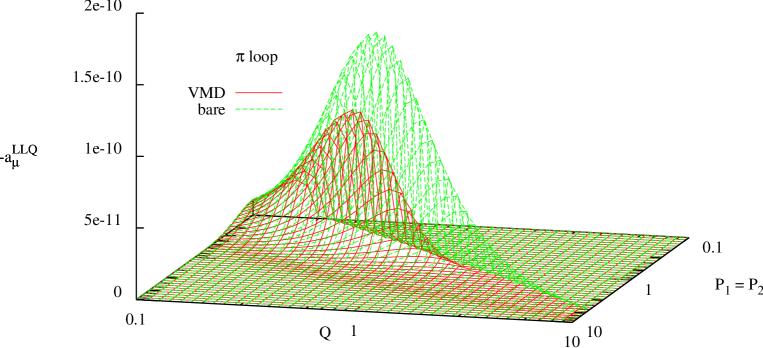
Figure 6: The momentum dependence of the pion loop contribution. Plotted is $a_{\mu}^{LLQ}$ of (20) as a function of $P_{1}=P_{2}$ and $Q$. Top surface: sQED, bottom surface:full VMD.

The other main evaluation of the pion-loop in [14, 15] (HKS) used a different approach. It was believed then that the full VMD approach did not respect gauge invariance. HKS therefore used the hidden local symmetry model with only vector mesons (HLS) [43] and obtained $-0.45\times 10^{-10}$. The only difference with full VMD is in the $\pi\pi\gamma^{*}\gamma^{*}$ as discussed in [18]. In [18] it was shown that the full VMD approach is gauge invariant. However, the large spread in the results for models that are rather similar was puzzling, both have a good description of the pion form-factor. We can make a similar study of the momentum range contributions, shown in Fig. 7.

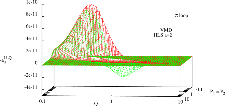
Figure 7: $-a_{\mu}^{LLQ}$ of (20) as a function of $P_{1}=P_{2}$ and $Q$. Top surface: full VMD, bottom surface: HLS.

It is clearly visible that the two models agree very well for low momenta but there is a surprisingly large dip of the opposite sign for the HLS model at higher momenta, above and around 1 GeV. This is the reason for the large difference in the final number for $a_{\mu}^{\pi loop}$. A comparison as a function of the cut-off can be found in [39].

4.1.1 Short distance constraint: VMD is better

In QCD we know that the total hadronic contribution to the muon anomalous magnetic moment must be finite. This is however not necessarily true when looking at non-renormalizable models that in addition only describe part of the total hadronic contribution. For these one has too apply them intelligently, i.e. only use them in momentum regions where they are valid.

One tool to study possible regions of validity is to check how well the models do in reproducing short-distance constraints following directly from QCD. Examples of these are the Weinberg sum rules but there are also some applicable to more restricted observables. Unfortunately it is known that in general one cannot satisfy all QCD constraints with a finite number of hadrons included as discussed in detail in [44]. Still one wants to include as much as possible of QCD knowledge in the models used.

One constraint on the amplitude for $\gamma^{*}\gamma^{*}\to\pi\pi$ can be easily derived analoguously to the short-distance constraint of [21] for the pion exchange contribution. If we take both photons to be far off-shell and at a similar $Q^{2}$ then the leading term in the operator product expansion of the two electromagnetic currents is proportional to the axial current. However, a matrix element of the axial current with two pions vanishes so we have the constraint

$$\lim_{Q^{2}\to\infty}A(\gamma^{*}(q_{1}=Q+k)\gamma^{*}(q_{2}=-Q+k)\to\pi(p_{1})\pi(p_{2}))\propto\frac{1}{Q^{2}}$$ (21)

when all scalar products involving $k,p_{1},p_{2}$ and at most one power of Q are small compared to $Q^{2}$.

In scalar QED the amplitude for $\gamma^{*}\gamma^{*}\to\pi\pi$ is

$$ie^{2}\left[2g^{\mu\nu}+\frac{(k^{\mu}+Q^{\mu}-2p_{1}^{\mu})(k^{\nu}-Q^{\nu}-2p_{2}^{\nu})}{(Q+k-p_{1})^{2}-m_{\pi}^{2}}+\frac{(k^{\mu}+Q^{\mu}-2p_{2}^{\mu})(k^{\nu}-Q^{\nu}-2p_{1}^{\nu})}{(Q-k+p_{1})^{2}-m_{\pi}^{2}}\right]$$ (22)

which to lowest order in $1/Q^{2}$ is

$$2ie^{2}\left[g^{\mu\nu}-\frac{Q^{\mu}Q^{\nu}}{Q^{2}}\right].$$ (23)

This amplitude does not vanish in the large $Q^{2}$ limit. sQED does not satsify the short distance constraint.

In full VMD the $\gamma\pi\pi$ and $\gamma\gamma\pi\pi$ vertices of scalar QED are multiplied by a factor

$$\frac{m_{\rho}^{2}g^{\mu\nu}-q^{\mu}q^{\nu}}{m_{\rho}^{2}-q^{2}}$$ (24)

for each photon line, where $q$ is the momentum of the photon. The $(Q^{2})^{0}$ term in the $\gamma^{*}\gamma^{*}\to\pi\pi$ amplitude is then zero. The full VMD model does respect the short distance constraint.

In HLS the $\gamma\pi\pi$ vertex of scalar QED is multiplied by

$$g^{\mu\nu}-\frac{a}{2}\frac{q^{2}g^{\mu\nu}-q^{\mu}q^{\nu}}{q^{2}-m_{\rho}^{2}}$$ (25)

and the $\gamma\gamma\pi\pi$ vertex is multiplied by

$$g^{\mu\alpha}g^{\nu\beta}-g^{\mu\alpha}\frac{a}{2}\frac{q^{2}g^{\nu\beta}-q^{\nu}q^{\beta}}{q^{2}-m_{\rho}^{2}}-g^{\nu\beta}\frac{a}{2}\frac{p^{2}g^{\mu\alpha}-p^{\mu}p^{\alpha}}{p^{2}-m_{\rho}^{2}}.$$ (26)

To lowest order in $1/Q^{2}$ the amplitude for $\gamma^{*}\gamma^{*}\to\pi\pi$ is

$$2ie^{2}\left[g^{\mu\nu}-\frac{Q^{\mu}Q^{\nu}}{Q^{2}}\right](1-a).$$ (27)

The HLS model with its usual value of $a=2$ does not satisfy the short distance constraint.

It was also noticed [22] in a similar vein that the ENJL model, that essentially has full VMD, lives up to the Weinberg sum rules but the HLS does not.

In fact, using the HLS with an unphysical value of the parameter $a=1$ satisfies the short-distance constraint (21) and lives up to the first Weinberg sum rule. The total result for that model is $a_{\mu}^{\pi loop}=-2.1\cdot 10^{-10}$, similar to the ENJL model. A comparison for different momentum regions between the full VMD model and a HLS model with $a=1$ is shown in Fig. 8.

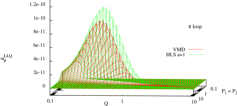
Figure 8: The momentum dependence of the pion loop contribution. $-a_{\mu}^{LLQ}$ of (20) as a function of $P_{1}=P_{2}$ and $Q$. Top surface: HLS a=1, bottom surface: full VMD.

Notice in particular that the part with the opposite sign from Fig. 7 has disappeared.

From this we conclude that a number in the range $a_{\mu}^{\pi loop}=-(1.5$-$2.1)\times 10^{-10}$ would be more appropriate.

4.2 Including polarizability at low energies

It was pointed out that the effect of pion polarizability was neglected in the estimates of the pion-loop in [14, 15, 17, 18] and a first estimate of this effect was given using the Euler-Heisenberg four photon effective vertex produced by pions [35] within Chiral Perturbation Theory. This approximation is only valid below the pion mass. In order to check the size of the pion radius effect and the polarizability, we have implemented the low energy part of the four-point function and computed $a_{\mu}^{LLQ}$ for these cases in Chiral Perturbation Theory (ChPT). First results were shown in [37, 39]. The plots shown include the $p^{4}$ result which is the same as the bare pion-loop and we include in the vertices the effect of the terms from the $L_{9}$ and $L_{10}$ terms in the $p^{4}$ ChPT Lagrangian. The effect of the charge radius is shown in Fig. 9 compared to the VMD parametrization of it, notice the different momentum scales compared to the earlier Figs. 6-8. The polarizability we have set to zero by setting $L_{9}+L_{10}=0$. As expected, the charge radius effect is included in the VMD result since the latter gives a good description of the pion form-factor.

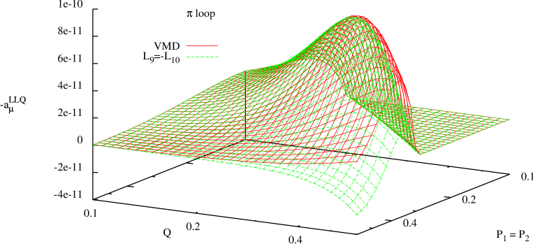
Figure 9: $-a_{\mu}^{LLQ}$ of (20) as a function of $P_{1}=P_{2}$ and $Q$. Top surface: full VMD, bottom surface: ChPT with $L_{9}=-L_{10}$ so the charge radius is included but no polarizability.

Including the effect of the polarizability can be done in ChPT by using experimentally determined values for $L_{9}$ and $L_{10}$. The latter can be determined from $\pi^{+}\to e\nu\gamma$ or the hadronic vector two-point functions. Both are in good agreement and lead to a prediction of the pion polarizability confirmed by the Compass experiment [45]. The effect of including this in ChPT on $a_{\mu}^{LLQ}$ is shown in Fig. 10. An increase of 10-15% over the VMD estimate can be seen.

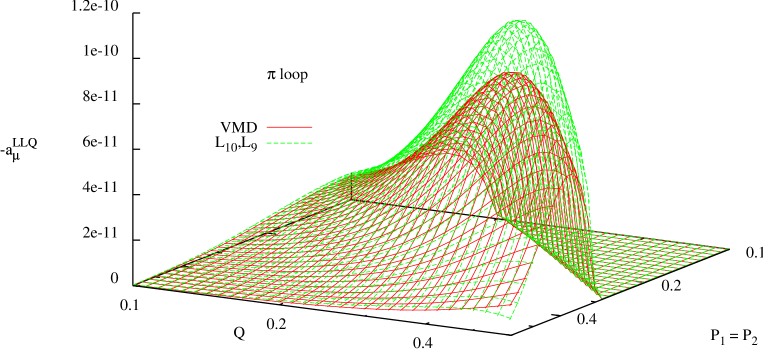
Figure 10: $-a_{\mu}^{LLQ}$ of (20) as a function of $P_{1}=P_{2}$ and $Q$. Bottom surface: full VMD, top surface: ChPT with $L_{9}\neq-L_{10}$ so the charge radius and the polarizability are included.

ChPT at lowest order, or $p^{4}$, for $a_{\mu}$ is just the point-like pion loop or sQED. At NLO pion exchange with point-like vertices and the pion-loop calculated at NLO in ChPT are needed. Both give divergent contributions to $a_{\mu}$, so pure ChPT is of little use in predicting $a_{\mu}$. If we had tried to extend the plots in Figs. 9 and 10 to higher momenta the bad high energy behaviour would have been clearly visible. We therefore need to go beyond ChPT. This is done in the next subsection.

4.3 Including polarizability at higher energies

If we want to see the full effect of the polarizability we need to include a model that can be extended all the way, or at least to a cut-off of about 1 GeV. For the approach of [35] this was done in [36] by including a propagator description of $a_{1}$ and choosing it such that the full contribution of the pion-loop to $a_{\mu}$ is finite. They obtained a range of $-(1.1$-$7.1)\times 10^{-10}$ for the pion-loop contribution. This seems a very broad range when compared with all earlier estimates. One reason is that the range of polarizabilities used in [36] is simply not compatible with ChPT. The pion polarizability is an observable where ChPT should work and indeed the convergence is excellent. The ChPT prediction has also recently been confirmed by experiment [45]. Our work discussed below indicates that $-(2.0\pm 0.5)\times 10^{-10}$ is a more appropriate range for the pion-loop contribution.

The polarizability comes from $L_{9}+L_{10}$ in ChPT [46, 47]. Using [48], we notice that the polarizability is produced by $a_{1}$-exchange depicted in Fig. 11. This is depicted in the left diagram of Fig. 11.

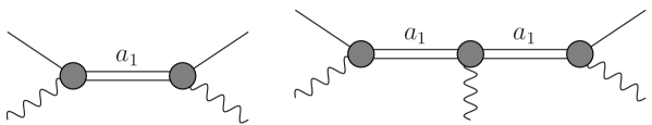
Figure 11: Left: the $a_{1}$-exchange that produces the pion polarizability. Right: an example of a diagram that is required by gauge invariance.

However, once such an exchange is there, diagrams like the right one in Fig. 11 lead to effective $\pi\pi\gamma\gamma\gamma$ vertices and are required by electromagnetic gauge invariance. This issue can be dealt with in several ways. Ref. [36] introduced modifications of the $a_{1}$ propagator that introduces one form of the extra vertices. We deal with them via effective Lagrangians incorporating vector and axial-vector mesons.

If one studies Fig. 11 one could raise the question “Is including a $\pi$-loop but no $a_{1}$-loop consistent?” The answer is yes with the following argument. We can first look at a tree level Lagrangian including pions $\rho$ and $a_{1}$. We then integrate out the $\rho$ and $a_{1}$ and calculate the one-loop pion diagrams with the resulting all order Lagrangian. In the diagrams of the original Lagrangian this corresponds to only including loops with at least one pion propagator present. Numerical results for cases including full $a_{1}$ loops are presented as well below. As a technicality, we use anti-symmetric vector fields for the vector and axial-vector mesons. This avoids complications due to $\pi$-$a_{1}$ mixing. We add vector $V_{\mu\nu}$ and axial-vector $A_{\mu\nu}$ nonet fields. The kinetic terms are given by [48]

$$-\frac{1}{2}\left\langle\nabla^{\lambda}V_{\lambda\mu}\nabla_{\nu}V^{\nu\mu}-\frac{M_{V}^{2}}{2}V_{\mu\nu}V^{\mu\nu}\right\rangle+V\leftrightarrow A\,.$$ (28)

We add first the terms that contribute to the $L_{i}$ [48]

$$\frac{F_{V}}{2\sqrt{2}}\left\langle f_{+\mu\nu}V^{\mu\nu}\right\rangle+\frac{iG_{V}}{\sqrt{2}}\left\langle V^{\mu\nu}u_{\mu}u_{\nu}\right\rangle+\frac{F_{A}}{2\sqrt{2}}\left\langle f_{-\mu\nu}A^{\mu\nu}\right\rangle$$ (29)

with $L_{9}=\frac{F_{V}G_{V}}{2M_{V}^{2}}$, $L_{10}=-\frac{F_{V}^{2}}{4M_{V}^{2}}+\frac{F_{A}^{2}}{4M_{A}^{2}}$. The Weinberg sum rules in the chiral limit imply $F_{V}^{2}=F_{A}^{2}+F^{2}_{\pi}$, $F_{V}^{2}M_{V}^{2}=F_{A}^{2}M_{A}^{2}$ and requiring VMD behaviour for the pion form-factor $F_{V}G_{V}=F^{2}_{\pi}$. We have used input values for the $L_{9}$ and $L_{10}$ consistent with this in the previous subsection.

Calculating the $\gamma^{*}\gamma^{*}\to\pi\pi$ amplitude in this framework using antisymmetric tensor notation to lowest order in $1/Q^{2}$ gives the amplitude

$$2ie^{2} \frac{F_{A}^{2}}{Q_{1}^{2}m_{a}^{2}F^{2}}(-p_{1}^{\mu}Q_{1}^{\nu}p_{1}\cdot Q_{1}-p_{1}^{\nu}Q_{1}^{\mu}p_{1}\cdot Q_{1}+Q_{1}^{\mu}Q_{1}^{\nu}m_{\pi}^{2}+g^{\mu\nu}(p_{1}\cdot Q_{1})^{2})$$

$$+2ie^{2} \frac{F_{A}^{2}}{m_{a}^{2}F^{2}}(p_{1}^{\mu}p_{1}^{\nu}-g^{\mu\nu}m_{\pi}^{2})$$

$$+2ie^{2} (F_{A}^{2}+F^{2}-F_{V}^{2})\left(\frac{g^{\mu\nu}}{F^{2}}-\frac{Q_{1}^{\mu}Q_{1}^{\nu}}{Q_{1}^{2}F^{2}}\right).$$ (30)

The last line vanishes for $F_{A}^{2}+F^{2}-F_{V}^{2}=0$ which is one of Weinberg’s sum rules. However, the first two lines give the additional requirement $F_{A}^{2}=0$. In this model it is not possible to incorporate the $a_{1}$ meson and satisfy the short distance constraint (21).

First, we take the model with only $\pi$ and $\rho$, i.e. we only keep the first two terms of (28) and (29). The one-loop contributions to $\Pi^{\rho\nu\alpha\beta}$ are not finite. They were also not finite for the HLS model of HKS, but the relevant $\delta\Pi^{\rho\nu\alpha\beta}/\delta p_{3\lambda}$ was. However, in the present model, the derivative can be made finite only for $G_{V}=F_{V}/2$. With this value of the parameters the result for $a_{\mu}$ is identical to that of the HLS model and suffers as a consequences from the same defects discussed above.

Next we do add the $a_{1}$ and require $F_{A}\neq 0$. After a lot of work we find that $\delta\Pi^{\rho\nu\alpha\beta}/\delta p_{3\lambda}|_{p_{3}=0}$ is finite only for $G_{V}=F_{V}=0$ and $F_{A}^{2}=-2F_{\pi}^{2}$ or, if including a full $a_{1}$-loop $F_{A}^{2}=-F_{\pi}^{2}$. These solutions are clearly unphysical.

We then add all $\rho a_{1}\pi$ vertices given by

$$\lambda_{1}\left\langle\left[V^{\mu\nu},A_{\mu\nu}\right]\chi_{-}\right\rangle+\lambda_{2}\left\langle\left[V^{\mu\nu},A_{\nu\alpha}\right]{h_{\mu}}^{\nu}\right\rangle$$

$$+\lambda_{3}\left\langle i\left[\nabla^{\mu}V_{\mu\nu},A_{\nu\alpha}\right]u_{\alpha}\right\rangle+\lambda_{4}\left\langle i\left[\nabla_{\alpha}V_{\mu\nu},A_{\alpha\nu}\right]u^{\mu}\right\rangle$$

$$+\lambda_{5}\left\langle i\left[\nabla^{\alpha}V_{\mu\nu},A_{\mu\nu}\right]u_{\alpha}\right\rangle+\lambda_{6}\left\langle i\left[V^{\mu\nu},A_{\mu\nu}\right]{{f_{-}}^{\alpha}}_{\nu}\right\rangle$$

$$+\lambda_{7}\left\langle iV_{\mu\nu}A^{\mu\rho}{A^{\nu}}_{\rho}\right\rangle\,.$$ (31)

These are not all independent due to the constraints on $V_{\mu\nu}$ and $A_{\mu\nu}$ [49], there are three relations. After a lot of work, we found that no solutions with $\delta\Pi^{\rho\nu\alpha\beta}/\delta p_{3\lambda}|_{p_{3}=0}$ exists except those already obtained without $\Lambda_{i}$ terms. The same conclusions holds if we look at the combination that shows up in the integral over $P_{1}^{2},P_{2}^{2},Q^{2}$. We thus find no reasonable model that has a finite prediction for $a_{\mu}$ for the pion-loop including $a_{1}$. In the remainder we therefore stick to $\lambda_{i}=0$ for the numerical results.

Let us first show the result for one of the finite cases, no $a_{1}$ loop, $F_{V}=G_{V}=0$ and $F_{A}^{2}=-2F_{\pi}^{2}$. The resulting contribution from the different momentum regimes is shown in Fig. 12

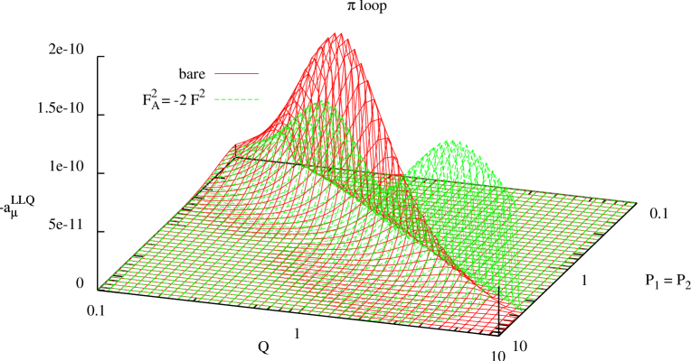
Figure 12: $-a_{\mu}^{LLQ}$ as defined in (20) as a function of $P_{1}=P_{2}$ and $Q$ with $a_{1}$ but no full $a_{1}$-loop, $F_{A}^{2}=-2F_{\pi}^{2}$ and $F_{V}=G_{V}=0$. The bare pion loop is shown for comparison.

The high-energy behaviour is by definition finite but there is a large bump at rather high energies. The other finite solution, including a full $a_{1}$-loop and $F_{A}=-F_{\pi}^{2},F_{V}=G_{V}=0$ is shown in Fig. 13.

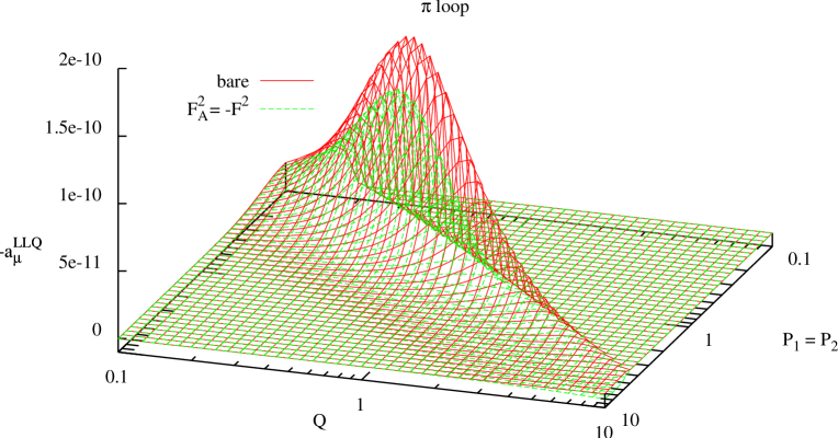
Figure 13: $-a_{\mu}^{LLQ}$ as defined in (20) as a function of $P_{1}=P_{2}$ and $Q$ with $a_{1}$ with a full $a_{1}$-loop, $F_{A}^{2}=-F_{\pi}^{2}$ and $F_{V}=G_{V}=0$. The bare pion loop is shown for comparison.

Here the funny bump at high energies has disappeared but the behaviour is still unphysical. The high-energy behaviour is good by definition since we enforced a finite $a_{\mu}$.

We can now look at the cases where $a_{\mu}^{\pi loop}$ was not finite but that include a good low-energy behaviour. I.e. they have $F_{V}^{2}=F_{\pi}^{2}/2$, $F_{V}G_{V}=F_{\pi}^{2}$, $F_{A}^{2}=F_{\pi}^{2}/2$ and $M_{A}^{2}=2M_{V}^{2}$. The resulting model then satisfies the Ward identities and the VMD behaviour of the pion-form factor. For the case with no $a_{1}$-loop we obtain $-a_{\mu}^{LLQ}$ as shown in Fig. 14.

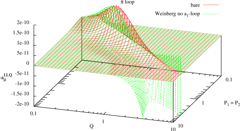
Figure 14: $-a_{\mu}^{LLQ}$ as defined in (20) as a function of $P_{1}=P_{2}$ and $Q$ with $a_{1}$ but no full $a_{1}$-loop. Parameters determined by the Weinberg sum rules.

The bad high energy behaviour is clearly visible, but it only starts above 1 GeV. The same input parameters but with a full $a_{1}$-loop leads to only small changes in the momentum regime considered as shown in Fig. 15

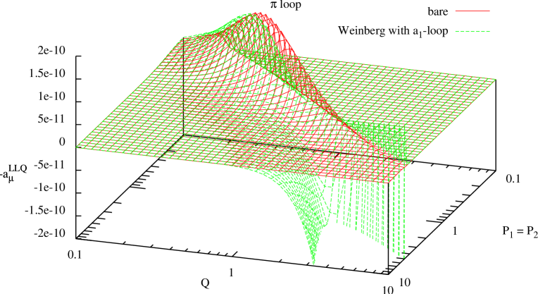
Figure 15: $-a_{\mu}^{LLQ}$ as defined in (20) as a function of $P_{1}=P_{2}$ and $Q$ with $a_{1}$ but no full $a_{1}$-loop. Parameters determined by the Weinberg sum rules.

Again the bad high-energy behaviour is clearly visible.

As a last model, we take the case with $F_{A}^{2}=+F_{\pi}^{2}$ and add VMD propagators also in the photons coming from vertices involving $a_{1}$. This makes the model satisfy the short-distance constraint (21). The contributions to $a_{\mu}^{\pi loop}$ are shown in Fig. 16.

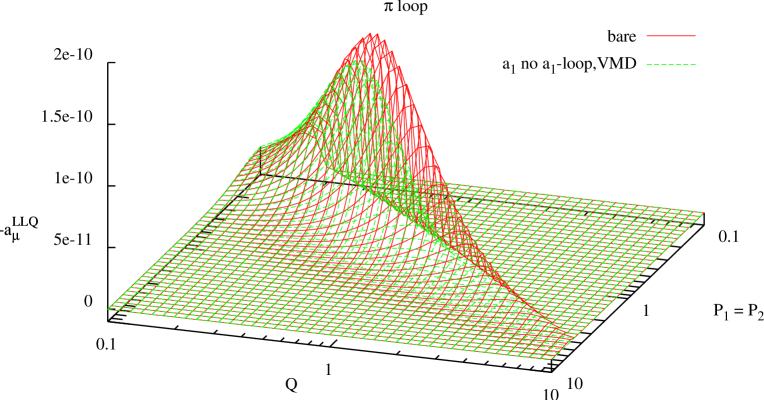
Figure 16: $-a_{\mu}^{LLQ}$ as defined in (20) as a function of $P_{1}=P_{2}$ and $Q$ with $a_{1}$ and $F_{A}^{2}=F_{\pi}^{2}$ but no full $a_{1}$-loop. A VMD form-factor is added in all photon legs.

The same model but now with the full $a_{1}$-loop is shown in Fig. 17.

Figure 17: $-a_{\mu}^{LLQ}$ as defined in (20) as a function of $P_{1}=P_{2}$ and $Q$ with $a_{1}$ and $F_{A}^{2}=F_{\pi}^{2}$ with a full $a_{1}$-loop. A VMD form-factor is added in all photon legs.

Both cases are very similar and here is a good high energy behaviour due to the VMD propagators added. This model cannot be reproduced by the Lagrangians shown above, we need higher order terms to do so. However, the arguments of [18] showing that the full VMD model was gauge invariant also apply to this model.

Now how does the full contribution to $a_{\mu}^{\pi loop}$ of these various models look like. The integrated contribution up to a maximum $\Lambda$ for the size of $P_{1},P_{2}$ and $Q$ is shown in Fig. 18.

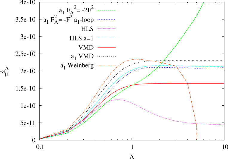
Figure 18: $-a_{\mu}$ using a variety of models for the pion loop as a function of $\Lambda$, the cut-off on the photon momenta. Units for $\Lambda$ are GeV.

The models with good high energy behaviour are the ones with a horizontal behaviour towards the right. We see that the HLS is quite similar to the others below about 0.5 GeV but then drops due to the part with the sign as shown in Fig. 7. All physically acceptable models that show a reasonable enhancement over the full VMD result. In fact, all models except HLS end up with a value of $a_{\mu}=-(2.0\pm 0.5)\times 10^{-10}$ when integrated up-to a cut-off of order 1-2 GeV. We conclude that that is a reasonable estimate for the pion-loop contribution.

We have not redone the calculation with the model of [36], however their large spread of numbers comes from considering a very broad range of pion polarizabilities and we suspect that the result might contain a large contribution from high energies similarly to the model shown in Fig. 12. We therefore feel that their broad range should be discarded.

5 Summary and conclusions

In this paper we have two main results and two smaller ones. The first main result is that we expect large and opposite sign contribution from the disconnected versus the connected parts in lattice calculations of the HLbL contribution to the muon anomalous magnetic moment.

The second main result is that the estimate of the pion-loop is

$$a_{\mu}^{\pi loop}=-(2.0\pm 0.5)\cdot 10^{-10}\,.$$ (32)

This contains the effects of the pion polarizability as well as estimates of other $a_{1}$ effects. The main constraints are that a realistic limit to low-energy ChPT seems to constrain the models enough to provide the result and range given in (32). We have given a number of arguments why the HLS number of [14, 15] should be considered obsolete. In this context we have also derived a short distance constraint on the underlying $\pi\pi\gamma^{*}\gamma^{*}$ amplitude.

As a minor result we have given the extension of the Gegenbauer polynomial method of [20, 9] to the most general hadronic vector four-point function.

References

- [1] G. W. Bennett et al. [Muon g-2 Collaboration], Phys. Rev. Lett. 89 (2002) 101804 [Erratum-ibid. 89 (2002) 129903] [hep-ex/0208001].
- [2] G. W. Bennett et al. [Muon g-2 Collaboration], Phys. Rev. Lett. 92 (2004) 161802 [hep-ex/0401008].
- [3] G. W. Bennett et al. [Muon G-2 Collaboration], Phys. Rev. D 73 (2006) 072003 [hep-ex/0602035].
- [4] J. Beringer et al. [Particle Data Group Collaboration], Phys. Rev. D 86 (2012) 010001.
- [5] R. M. Carey, K. R. Lynch, J. P. Miller, B. L. Roberts, W. M. Morse, Y. K. Semertzides, V. P. Druzhinin and B. I. Khazin et al., FERMILAB-PROPOSAL-0989.
- [6] H. Iinuma [J-PARC New g-2/EDM experiment Collaboration], J. Phys. Conf. Ser. 295 (2011) 012032.
- [7] M. Knecht, Lect. Notes Phys. 629 (2004) 37 [hep-ph/0307239].
- [8] J. P. Miller, E. de Rafael and B. L. Roberts, Rept. Prog. Phys. 70 (2007) 795 [hep-ph/0703049].
- [9] F. Jegerlehner and A. Nyffeler, Phys. Rept. 477 (2009) 1 [arXiv:0902.3360 [hep-ph]].
- [10] M. Benayoun et al., arXiv:1407.4021 [hep-ph].
- [11] G. D’Ambrosio, M. Iacovacci, M. Passera, G. Venanzoni, P. Massarotti and S. Mastroianni, EPJ Web Conf. 118 (2016).
- [12] T. Kinoshita, B. Nizic and Y. Okamoto, Phys. Rev. D 31 (1985) 2108.
- [13] E. de Rafael, Phys. Lett. B 322 (1994) 239 [hep-ph/9311316].
- [14] M. Hayakawa, T. Kinoshita and A. I. Sanda, Phys. Rev. Lett. 75 (1995) 790 [hep-ph/9503463].
- [15] M. Hayakawa, T. Kinoshita and A. I. Sanda, Phys. Rev. D 54 (1996) 3137 [hep-ph/9601310].
- [16] M. Hayakawa and T. Kinoshita, Phys. Rev. D 57 (1998) 465 [hep-ph/9708227] [Erratum-ibid. D 66 (2002) 019902, [hep-ph/0112102]].
- [17] J. Bijnens, E. Pallante and J. Prades, Phys. Rev. Lett. 75 (1995) 1447 [Erratum-ibid. 75 (1995) 3781] [hep-ph/9505251].
- [18] J. Bijnens, E. Pallante and J. Prades, Nucl. Phys. B 474 (1996) 379 [hep-ph/9511388].
- [19] J. Bijnens, E. Pallante and J. Prades, Nucl. Phys. B 626 (2002) 410 [hep-ph/0112255].
- [20] M. Knecht and A. Nyffeler, Phys. Rev. D 65 (2002) 073034 [hep-ph/0111058].
- [21] K. Melnikov and A. Vainshtein, Phys. Rev. D 70 (2004) 113006 [hep-ph/0312226].
- [22] J. Bijnens and J. Prades, Mod. Phys. Lett. A 22 (2007) 767 [hep-ph/0702170].
- [23] J. Prades, E. de Rafael and A. Vainshtein, (Advanced series on directions in high energy physics. 20) [arXiv:0901.0306 [hep-ph]].
- [24] C. S. Fischer, T. Goecke and R. Williams, Eur. Phys. J. A 47 (2011) 28 [arXiv:1009.5297 [hep-ph]].
- [25] T. Goecke, C. S. Fischer and R. Williams, Phys. Rev. D 83 (2011) 094006 [arXiv:1012.3886 [hep-ph]].
- [26] T. Goecke, C. S. Fischer and R. Williams, Phys. Rev. D 87 (2013) 034013 [arXiv:1210.1759 [hep-ph]].
- [27] G. Eichmann, C. S. Fischer, W. Heupel and R. Williams, AIP Conf. Proc. 1701 (2016) 040004 doi:10.1063/1.4938621 [arXiv:1411.7876 [hep-ph]].
- [28] G. Colangelo, M. Hoferichter, M. Procura and P. Stoffer, JHEP 1409 (2014) 091 doi:10.1007/JHEP09(2014)091 [arXiv:1402.7081 [hep-ph]].
- [29] G. Colangelo, M. Hoferichter, B. Kubis, M. Procura and P. Stoffer, Phys. Lett. B 738 (2014) 6 doi:10.1016/j.physletb.2014.09.021 [arXiv:1408.2517 [hep-ph]].
- [30] G. Colangelo, M. Hoferichter, M. Procura and P. Stoffer, JHEP 1509 (2015) 074 doi:10.1007/JHEP09(2015)074 [arXiv:1506.01386 [hep-ph]].
- [31] V. Pauk and M. Vanderhaeghen, Phys. Rev. D 90 (2014) no.11, 113012 doi:10.1103/PhysRevD.90.113012 [arXiv:1409.0819 [hep-ph]].
- [32] T. Blum, N. Christ, M. Hayakawa, T. Izubuchi, L. Jin and C. Lehner, Phys. Rev. D 93 (2016) no.1, 014503 doi:10.1103/PhysRevD.93.014503 [arXiv:1510.07100 [hep-lat]].
- [33] J. Green, O. Gryniuk, G. von Hippel, H. B. Meyer and V. Pascalutsa, Phys. Rev. Lett. 115 (2015) no.22, 222003 doi:10.1103/PhysRevLett.115.222003 [arXiv:1507.01577 [hep-lat]].
- [34] T. Blum et al, present by L. Jin at Lattice 2016
- [35] K. T. Engel, H. H. Patel and M. J. Ramsey-Musolf, Phys. Rev. D 86 (2012) 037502 doi:10.1103/PhysRevD.86.037502 [arXiv:1201.0809 [hep-ph]].
- [36] K. T. Engel and M. J. Ramsey-Musolf, Phys. Lett. B 738 (2014) 123 doi:10.1016/j.physletb.2014.09.006 [arXiv:1309.2225 [hep-ph]].
- [37] J. Bijnens and M. Z. Abyaneh, EPJ Web Conf. 37 (2012) 01007 [arXiv:1208.3548 [hep-ph]].
- [38] J. Bijnens, EPJ Web Conf. 118 (2016) 01002 doi:10.1051/epjconf/201611801002 [arXiv:1510.05796 [hep-ph]].
- [39] M. Z. Abyaneh, “The Anatomy of the Pion Loop Hadronic Light by Light Scattering Contribution to the Muon Magnetic Anomaly,” arXiv:1208.2554 [hep-ph], master thesis.
- [40] M. Hayakawa, T. Blum, N. H. Christ, T. Izubuchi, L. C. Jin and C. Lehner, PoS LATTICE 2015 (2016) 104 [arXiv:1511.01493 [hep-lat]].
- [41] J. Aldins, S. J. Brodsky, A. J. Dufner and T. Kinoshita, , Phys. Rev. D 1 (1970) 2378.
- [42] M. Procura, G. Colangelo, M. Hoferichter and P. Stoffer, EPJ Web Conf. 118 (2016) 01030. doi:10.1051/epjconf/201611801030
- [43] M. Bando, T. Kugo and K. Yamawaki, Phys. Rept. 164 (1988) 217. doi:10.1016/0370-1573(88)90019-1
- [44] J. Bijnens, E. Gamiz, E. Lipartia and J. Prades, JHEP 0304 (2003) 055 [hep-ph/0304222].
- [45] C. Adolph et al. [COMPASS Collaboration], Phys. Rev. Lett. 114, 062002 (2015) [arXiv:1405.6377 [hep-ex]].
- [46] J. F. Donoghue and B. R. Holstein, Phys. Rev. D 48 (1993) 137 doi:10.1103/PhysRevD.48.137 [hep-ph/9302203].
- [47] J. Bijnens and F. Cornet, Nucl. Phys. B 296 (1988) 557. doi:10.1016/0550-3213(88)90032-6
- [48] G. Ecker, J. Gasser, A. Pich and E. de Rafael, Nucl. Phys. B 321, 311 (1989).
- [49] S. Leupold, private communication.