Decoupling Jupiter’s deep and atmospheric flows using the upcoming Juno gravity measurements and a dynamical inverse model

Abstract

Observations of the flow on Jupiter exists essentially only for the cloud-level, which is dominated by strong east-west jet-streams. These have been suggested to result from dynamics in a superficial thin weather-layer, or alternatively be a manifestation of deep interior cylindrical flows. However, it is possible that the observed winds are indeed superficial, yet there exists deep flow that is completely decoupled from it. To date, all models linking the wind, via the induced density anomalies, to the gravity field, to be measured by Juno, consider only flow that is a projection of the observed could-level wind. Here we explore the possibility of complex wind dynamics that include both the shallow weather-layer wind, and a deep flow that is decoupled from the flow above it. The upper flow is based on the observed cloud-level flow and is set to decay with depth. The deep flow is constructed to produce cylindrical structures with variable width and magnitude, thus allowing for a wide range of possible scenarios for the unknown deep flow. The combined flow is then related to the density anomalies and gravitational moments via a dynamical model. An adjoint inverse model is used for optimizing the parameters controlling the setup of the deep and surface-bound flows, so that these flows can be reconstructed given a gravity field. We show that the model can be used for examination of various scenarios, including cases in which the deep flow is dominating over the surface wind. We discuss extensively the uncertainties associated with the model solution. The flexibility of the adjoint method allows for a wide range of dynamical setups, so that when new observations and physical understanding will arise, these constraints could be easily implemented and used to better decipher Jupiter flow dynamics.

1 Introduction

The nature of the flow on Jupiter below the observed cloud-level is still mostly unknown. Analysis of the cloud-level flow, based on tracking of cloud observations (e.g., Porco et al., 2003), shows strong east-west flow of up to 140 m s^-1, with some local non zonal flows such as around the Great Red Spot. Below the cloud-level, the Galileo probe (Atkinson et al., 1996) showed winds of 160 m s^-1 going down to a depth of at least 24 bars at a specific location ($6^{\circ}$N), but it is questionable of whether this represents the general flow (Orton et al., 1998; Showman and Dowling, 2000). Some studies suggest, based on indirect observations, that non-zero winds should exist below the cloud-level (Conrath et al., 1981; Gierasch et al., 1986; Dowling and Ingersoll, 1988, 1989), but their conclusions were limited to a depth of less than 1% of the planet’s radius.

Theoretical understanding and numerical modeling during the past decades can be divided into two general mechanistic approaches. The first, assumes the flow is confined to a shallow region, close to the cloud-level, similar to atmospheres of terrestrial planets, and becomes organized into zonal jets due to atmospheric turbulence (Rhines, 1975, 1979). The energy source for the flow can then either come from internal heating or solar radiation. The mechanism governing such shallow zonal flows was suggested to be either turbulence forced from the lower layers (e.g., Williams, 1978, 2003; Showman, 2007; Kaspi and Flierl, 2007), or shallow decaying turbulence (e.g., Cho and Polvani, 1996; Scott and Polvani, 2007). Other studies, using idealized general circulation models solving for the full primitive equations, were even able to simulate cloud-level flow structures that are consistent with those observed in all solar system giant planets (Lian and Showman, 2010; Liu and Schneider, 2010). The second approach assumes that the observed cloud-level flow is a surface manifestation of convective columns originating from the hot interiors of the planet (Busse, 1976, 1994). Angular momentum conservation in a rapidly rotating planet like Jupiter leads the flow to be aligned with the direction of the spin axis, and it has been was shown in many studies that strong internal convection can lead to zonally symmetric flows aligned parallel to the axis of rotation (e.g., Aurnou and Olson, 2001; Christensen, 2002; Wicht et al., 2002; Heimpel et al., 2005; Kaspi et al., 2009; Jones and Kuzanyan, 2009; Gastine and Wicht, 2012; Gastine et al., 2013; Chan and Mayr, 2013). In all these studies, however, the width of the equatorial east to west super-rotation is much greater than that observed on Jupiter. These two approaches have been in debate for the last 40 years with no observed data that could resolve the controversy. A third option, not considered in previous studies, is that both type of flows exist alongside: an internal flow of an unknown character and likely forced by convection and shallow flow related to the observed cloud level winds. Such a scenario would require additional dynamics existing beneath the cloud level so that the weather-layer winds would decay with depth (e.g., due to latent heat release, or enhanced stratification at the radiative-convective boundary), while the deep winds will occupy the deep convective region which is unaffected by the solar radiation.

The expected gravity measurements of Jupiter by Juno might give additional information about the character of the flow. Starting in the fall of 2016, the Juno spacecraft will perform high accuracy gravity measurements, with sensitivity expected to allow measurements at least up to gravity harmonic $J_{10}$ (Bolton, 2005; Finocchiaro and Iess, 2010). Several studies have shown that these gravity measurements could be used to decipher the flow on the planet below its cloud-level (Hubbard, 1999; Kaspi et al., 2010). The assumption is that in the dynamical regime expected to govern the flow on the planet, the flow is accompanied by changes in the density field, so that, given the gravity measurements, a static density stratification together with a flow field could be found to best explain the measurements.

To date, most models linking the wind (via the induced density anomalies) to the gravity field to be measured by Juno, consider only flow that is a projection of the observed cloud-level wind (e.g., Hubbard, 1999; Kaspi et al., 2010; Kaspi, 2013; Zhang et al., 2015; Kaspi et al., 2016). Some assume full cylindrical flow while others allow for the wind to decay with depth. However, none of the models included the possibility of an internal flow that is decoupled from the surface-bound winds. In addition, these models were able to calculate the gravitational moments from a given flow field, but did not offer any methodology for the inverse problem. In another study (Galanti and Kaspi, 2016), an adjoint based inverse method was developed to relate the expected gravity measurements to the flow underneath the cloud-level. It was shown that given an measured gravity field the penetration depth of the observed could-level wind could be recovered, even in cases where this depth varies with latitude. The method also allows for measurement errors to be incorporated, and uncertainties in the solution could be calculated.

In this study, we explore the possibility of complex wind dynamics that include both the surface bound wind, and a deep flow that is completely detached from the flow above it. The methodology developed in this study is a continuation of that presented in Galanti and Kaspi (2016). There, the adjoint method was introduced and simple wind structures were simulated and then shown to be invertible by the adjoint model given the gravity moments. Here, we consider more complex flow cases, and rigorously quantify the uncertainty in the adjoint solution and the inevitability limits. The manuscript is organized as follows: in section 2 we describe the model and methods used to calculate the complex flow structures, in section 3 we discuss the various experiments performed, and conclusions are given in section 4.

2 Methods

2.1 The thermal wind model

The dynamical model relating the flow on Jupiter to the density and gravitational moments, is similar to the one used in Galanti and Kaspi (2016). The model relates the flow field to the density field via the thermal wind equation (Kaspi et al., 2010). It assumes the dynamics to be in the regime of small Rossby numbers, where the flow to leading order is in geostrophic balance, therefore thermal wind balance holds

$$\left(2\Omega\cdot\nabla\right)\left[\widetilde{\rho}\mathbf{u}\right]=\nabla\rho^{\prime}\times\mathbf{g_{0}},$$ (1)

where $\Omega$ is the planetary rotation rate, $\widetilde{\rho}(r)$ is the background density field, $\mathbf{u}(\mathbf{r})$ is the 3D velocity, $\mathbf{g_{0}}\left(r\right)$ is the mean gravity vector and $\rho^{\prime}\left(r,\theta\right)$ is the dynamical density anomaly (Pedlosky, 1987; Kaspi et al., 2009). The calculation takes advantage of a known mean static density $\widetilde{\rho}(r)$ and gravity $\mathbf{g_{0}}\left(r\right)$ , calculated using the method of Hubbard (1999). In this study we assume the flow is in the zonal direction only and does not vary with longitude, so that $\mathbf{u}=u(r,\theta)\hat{e}_{\phi}$. The model also assumes sphericity and excludes the effect of gravity anomalies induced by the density anomalies. These specific assumptions were shown to be a very good approximation of the full treatment of the equations, which includes these effects (Galanti et al., 2016). Moreover, the thermal wind model was also shown to be in good agreement with a more complete oblate potential theory model (Kaspi et al., 2016).

In the model used here, a modification was applied to the version used in Galanti and Kaspi (2016). In a recent study, Kong et al. (2016) showed that when asymmetry between the northern and southern hemisphere winds exists, a more accurate solution is achieved when solving separately for the two hemispheres. Following their conclusion, the numerical derivative in latitude (lhs of Eq. 1) is computed separately for the two hemispheres.

The dynamically induced gravitational moments are calculated using the density solution $\rho$’ from the thermal wind model, by integrating

$$J_{n}=-\frac{2\pi}{Ma^{n}}\intop_{0}^{a}r^{\prime n+2}dr^{\prime}\intop_{-1}^{1}P_{n}\left(\mu^{\prime}\right)\rho^{\prime}\left(r^{\prime},\mu^{\prime}\right)d\mu^{\prime},$$ (2)

where $M$ is the mass of Jupiter, $a$ is the planet radius, $P_{n}$ are the Legendre polynomials, and $\mu=\cos\theta$. In the experiments presented here we use the same model to generate both the ’observations’, denoted $J_{n}^{o}$, and the model solutions, denoted $J_{n}^{m}$.

2.2 Construction of the surface-bound flow and deep flow

For the upper surface bound flow (a flow that is manifested in the cloud-level winds), we follow here the methodology of Galanti and Kaspi (2016), in which the observed cloud-level winds are projected along cylinders parallel to the axis of rotation, and set to decay toward the high pressure interior. The zonal wind field has the general form

$$U_{{\rm{surf}}}\left(r,\theta\right)=u_{0}\exp\left(\frac{r-a}{H(\theta)}\right),$$ (3)

where $u_{0}\left(r,\theta\right)$ are the observed cloud-level zonal winds extended constantly along the direction of the axis of rotation, $a$ is the planet radius, and $H(\theta)$ is the latitudinal dependent e-folding decay depth of the cloud level wind. The latitude dependent $H$ is defined as a summation over Legendre polynomials

$$H\left(\theta\right)=\sum_{i=1}^{N_{H}}h_{i}P_{i-1}(\theta),$$ (4)

where $P_{i}(\theta)$ are the Legendre polynomials, $h_{i}$ are the coefficients by which the shape of $H(\theta)$ is determined, and $N_{H}$ is the number of functions to be used. Such formulation allows for a solution to be found separately for different spatial scales of the winds and its resulting gravity signals.

Next, we set a possible deep flow. The physical assumption taken is that the observed flow pattern follows cylinders parallel to the planet axis of rotation. This flow structure emerges in many studies in which a general circulation model was forced by an internal heat source (e.g., Heimpel and Gómez Pérez, 2011; Christensen, 2002; Kaspi et al., 2009). We also demand that no deep flow exists inside the cylinder whose radius equals the static core region assumed in the thermal wind model, i.e., when $l<\text{l}_{{\rm I}}$, where $l=r\cos(\theta)$ is the distance from the axis of rotation, and $l_{{\rm I}}=14,500$ km is the thermal wind model inner radius (see Fig. 1b). Similarly, we demand that no deep flow exits outside of $l_{{\rm O}}=60,000$ km (equivalent to cutoff at latitude 30), the distance from axis of rotation outside which the observed cloud level wind is dominating the interior and no decoupling exists. This ensures that the deep flow does not interfere with the strong surface jets in the equatorial region in cases where they extend deep. The deep flow is set as

$$U_{{\rm cyl}}(r,\theta) = \begin{cases}l<l_{{\rm I}}&0\\ l_{{\rm I}}<l<l_{{\rm O}}&\sum_{n=1}^{N_{U}}u_{n}\sin\left(\frac{n\pi(l-l_{{\rm I}})}{l_{{\rm O}}-l_{{\rm I}}}\right)\\ l>l_{{\rm O}}&0\end{cases},$$ (5)

where $u_{1},...,u_{{\rm N_{U}}}$ are the magnitudes assigned to the sinuous functions, and $N_{U}$ is the number of functions used. This gives a flow structure that is function of $l$ only, and whose value is zero at $l=l_{{\rm I}}$ and $l=l_{{\rm O}}$.

Next, we demand that the deep flow decay toward the interior with the function

$$D(r,\theta) = \frac{1}{2}\tanh\frac{r-r_{{\rm D}}}{\delta a_{{\rm D}}}+1,$$

where $r_{{\rm D}}$ is the decay depth, and $\delta a_{{\rm D}}=2000$ km is the decay scale. This enables the inclusion of a physical constraint that the deep flow decays below a certain depth.

Finally, we demand that the deep flow is completely decoupled from the surface-bound flow. For simplicity, we choose the decay function to complement the decay function of the surface wind (Eq. 3), so that the deep flow decays to zero at the planet surface. The total deep flow is set as

$$U_{{\rm deep}}(r,\theta) = D\cdot\left[1-\exp\left(\frac{r-a}{H(\theta)}\right)\right]\cdot U_{{\rm cyl}}.$$ (6)

Using Eqs. 3 and 6 we set the total simulated wind field

$$U = U_{{\rm surf}}(r,\theta)+U_{{\rm deep}}(r,\theta).$$ (7)

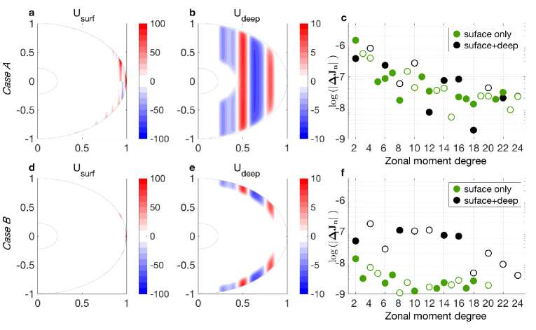
Figure 1: The simulated flow and resulting gravitational moments for case A (upper panels) and case B (lower panels). (a,d) Surface bound flow, (b,e) deep flow, and (c,f) the gravitational moments resulting from surface flow only (green dots), and combined surface and deep flow (black dots).

2.3 Simulated wind field and gravitational moments

Until the gravity observations from Juno will arrive, we can use the thermal wind model to simulate the observed field (Galanti and Kaspi, 2016) given a surface-bound wind and a deep flow. The free parameters adjustable when setting the total flow field are the depth of the surface wind $H(\theta)$ based on the coefficients $h_{i}$, the structure of the deep wind based on the coefficients $u_{i}$, and the depth of the deep flow $r_{{\rm D}}$. Using these parameters, we define two distinctly different scenarios, denoted as case A and case B. These cases are chosen to illustrate potential observations made by Juno.

In case A, we set the surface wind depth coefficients to $h_{1}=4000,\,h_{3}=-2000$ km (with all others set to zero). The deep flow coefficients are set to $u_{1}=1,\,u_{4}=5,\,u_{5}=-3,\,u_{8}=2$ m s^-1 (with all others set to zero). The depth of the deep flow is limited to be outside of $a_{{\rm D}}=30,000$ km from center of the planet. The resulting wind structure and the gravitational moments calculated using the thermal wind model are shown in Fig. 1a,b,c. The surface bound winds (Fig. 1a) are pronounced mostly in the equatorial region where they penetrate all the way to the equatorial plane. Its effect on the gravity moments (Fig. 1c, green dots) is substantial. The deep flow (Fig. 1b) has a structure of positive zonal velocity in the low latitudes, a width negative flow in the mid-latitudes, then again a strong positive flow in higher latitudes, and finally a weak negative jet in the high latitudes. Note that the strength of the deep flow is set to be an order of magnitude smaller than the surface winds. The effect of the deep flow on the gravitational moments is clear (Fig. 1c, black dots) - some the even moment values are increased (for example, $J_{4}$), while some values are decreased (for example, $J_{2}$), and in some cases the even the sign is changed (for example, $J_{8}$). Note that the odd moments ($J_{3,5,..})$ are not being modified by the deep flow, since it is symmetric between the northern and southern hemispheres.

In case B, we set the surface wind depth coefficients to be 10 times smaller than in case A. The result (Fig. 1d) is that the surface wind is strongly limited to the surface, and its affect on the gravitational moments is very small (Fig. 1f, green dots). The deep flow coefficients are set as in case A, but the depth of the deep flow is now limited to $a_{{\rm D}}=0.9a\eqsim 63,000$ km (Fig. 1e), thus confined to a much narrower region. The gravitational moments resulting from the deep flow (Fig. 1f, black dots) are smaller than in case A, but relative to the surface wind, the deep flow is now dominating the gravity field. We will use the total gravitational moments (black dots in Fig. 1c for case A, and those in Fig. 1f for case B) to simulate the observed field to be measured by Juno, and denote them $J_{{\rm n}}^{o}$.

2.4 Control variables and cost function definition

The control variables we aim to optimize are the parameters defining the depth of the surface wind $h_{1},...,h_{{\rm N_{H}}}$, the parameters defining the structure of the deep flow $u_{1},...,u_{{\rm N_{U}}}$, and the depth of the deep flow $a_{{\rm D}}$. Since each variable has different units, the problem is best conditioned when the total control vector is composed from the different parameters normalized by their typical values. We define the control vector as

$$\overrightarrow{\mathbf{X}_{{\rm C}}} = \left\{\left[h_{1},...,h_{{\rm N_{H}}}\right]/h_{{\rm nor}},\left[u_{1},...,u_{{\rm N_{U}}}\right]/u,a_{{\rm D}}/a_{{\rm nor}}\right\},$$

where $h_{{\rm nor}}=10^{7}$ m, $u_{{\rm nor}}=10$ m s^-2, and $a_{{\rm nor}}=10^{8}$ m. In the optimization procedure, the values of the normalized control variables are limited to the range of $-1$ to $1$, aside from the value for $a_{{\rm D}}/a_{{\rm nor}}$ is that limited between $0$ and $1$.

The cost function is defined similarly to Galanti and Kaspi (2016), as the weighted difference between the model calculated moments and those measured, with an additional penalty term that ensure that initial guess does not affect the solution

$$L = \mathbf{{\displaystyle\mathbf{\left(\mathbf{J^{m}}-\mathbf{J}^{o}\right)^{T}}W\left(\mathbf{J^{m}}-\mathbf{J}^{o}\right)}}+\epsilon\mathbf{X_{C}^{\mathbf{\mathbf{T}}}X_{\mathbf{\mathbf{C}}}},$$ (8)

where $\mathbf{J}^{\mathbf{\mathbf{m}}}$ is the $N$ size calculated model solution , $\mathbf{J}^{\mathbf{o}}$ is the observed one, and $\mathbf{W}$ is a diagonal matrix of size $N\times N$ with weights given to each moment $W_{ii}=4\times 10^{16}$, representing simulated uncertainties of $5\times 10^{-9}$. The second term in Eq. 8 act as a penalty term whose purpose is to ensure that the optimized solution is not affected by the initial guess, or any part of the control vector that do not affect the difference between the calculated and observed gravity moments. An extensive discussion of this issue (also known as the null space of the solution) can be found in Galanti et al. (2016). The value of the parameter $\epsilon$ is set according to the initial value of the cost function, so it affects the solution only when the cost function is reduced considerably. The form of the penalty term is set to penalize any non-zero value of the control variable $\mathbf{X_{C}}$ since we have no prior knowledge of either the depth of the surface bound wind.

2.5 Analysis of uncertainties in model solution

When estimating a solution for the gravity field that best matches the simulated (eventually, the observed) one, it is important to estimate the uncertainties associated with the solution. These uncertainties arise because the observations have uncertainties associated with them, and therefore the combined range of the observation uncertainties lead to uncertainties in the optimized variables. The control variable uncertainties are derived from the the Hessian matrix $\mathbf{G}$ (second derivative of the cost function $L$ with respect to the control vector $\mathbf{X}_{{\rm C}}$, see Galanti and Kaspi 2016). Inverting the Hessian matrix $\mathbf{G}$, we get the error covariance matrix $\mathbf{\mathbf{C}}$. This matrix includes the error covariance associated with combination of each two control variables (off diagonal terms), and the variance of each one (diagonal terms). Physically, the covariance matrix indicates to the formal uncertainties in the control variables given the uncertainties of the observations (weights $\mathbf{W}$ in the cost function). The larger the uncertainties in the observations are, the smaller are the weights in the cost function, and the larger the uncertainties in the control variables.

This information, however, does not give a direct estimate of the physical parameters we are interested in. For example, the depth of the surface wind (Eq. 4) is expressed in our calculations as a summation over Legendre polynomials whose coefficients are the control variables, and the information from the error covariance matrix $\mathbf{C}$ is about them. However, our interest is in the uncertainties associated with the depth of the surface wind as function of latitude so that the information from the error covariance matrix needs to be converted into information about the depth of the wind. Consider a case where no correlation exists between errors of one control parameter to another, so that the covariance matrix $\mathbf{C}$ has non zero values only on the diagonal, representing the variance of each control variable error. In such a case, one can generate many realizations of the errors, based on a normal distribution with standard deviation taken from the diagonal terms of $\mathbf{C}$. Using Eq. 4 these realizations can be converted to the depth of the wind at each latitude, so that for each latitude a distribution of errors is obtained. From that distribution an estimation of the error could be calculated, for example based on the $1^{th}$ standard deviation. However, in all experiments discussed in this study the off diagonal terms in $\mathbf{C}$ are substantial and cannot be neglected. Therefore, a method should be derived for how to generate realizations of the control variables errors, so that their covariance will satisfy $\mathbf{C}$.

By definition, the error covariance matrix has the form

$$\mathbf{C} \equiv \frac{\mathbf{X}\mathbf{X}^{T}}{N},$$ (9)

where $\mathbf{X}=\left\{\overrightarrow{\mathbf{X}_{1}},...,\overrightarrow{\mathbf{X}_{\mathbf{N}}}\right\}$ is the matrix whose rows contain $N$ realizations of the control variables errors. Eigen decomposing of $C$ gives

$$\mathbf{C} = \mathbf{S\Lambda}\mathbf{S}^{T},$$ (10)

where $S$ is the matrix composed from the eigenvectors, and $\Lambda$ is a matrix with the eigenvalues on its diagonal. Note that $S^{-1}=S^{T}$ since $C$ is positive definite. Using Eq. 9 we get

$$\mathbf{S}^{T}\mathbf{X}\mathbf{X}^{T}\mathbf{S} = \mathbf{\Lambda}N.$$ (11)

Defining a new set of error realizations $\mathbf{Y}=\left\{\overrightarrow{\mathbf{Y}_{1}},...,\overrightarrow{\mathbf{Y}_{N}}\right\}$ , such that $\mathbf{Y}=\mathbf{S}^{T}\mathbf{X}$, we get

$$\mathbf{Y}\mathbf{Y}^{T} = \mathbf{\Lambda}N,$$ (12)

so that the new control variable errors are uncorrelated.

We can now generate $N$ realizations, where each error is based on normal distribution with a standard deviation taken from $\Lambda$. Each realization $\overrightarrow{\mathbf{Y}_{i}}$ is then converted back to $\overrightarrow{\mathbf{X}_{i}}$ using $\overrightarrow{\mathbf{X}_{i}}=\mathbf{S}\overrightarrow{\mathbf{Y}_{i}}$. The number of realizations $N$ can be determined from the requirement that the realizations $\mathbf{X}$ satisfy Eq. 9 to a certain degree. Requiring that the difference between the first singular value of $C$ and the first singular value of $\mathbf{X}\mathbf{X}^{T}/N$ is less than one percent, we find that $N$ should be at least $500$. Note that an equivalent to this method would be to use a Monte-Carlo simulation to generate $\mathbf{X}$ directly based on $\mathbf{C}$, but that would be computationally less efficient.

These realizations $\mathbf{X}$, satisfying the full error covariance matrix $\mathbf{C}$, are converted to the actual physical variables using Eq. 4 for the depth of the surface wind

$$H_{i}^{{\rm err}}\left(\theta\right)=\sum_{j=1}^{N_{H}}h_{{\rm nor}}X_{i}(j)P_{j-1}(\theta),$$ (13)

and Eqs. 5 and 6 for the deep flow structure

$$U_{i}^{{\rm err}}(r,\theta) = \begin{cases}l<l_{{\rm I}}&0\\ l_{{\rm I}}<l<l_{{\rm O}}&D\cdot\left[1-\exp\left(\frac{r-a}{H(\theta)}\right)\right]\\ &\cdot\sum_{n=1}^{N_{U}}u_{{\rm nor}}X_{i}(n+N_{H})\\ &\sin\left(\frac{n\pi(l-l_{{\rm I}})}{l_{{\rm O}}-l_{{\rm I}}}\right)\\ l>l_{{\rm O}}&0\end{cases}.$$ (14)

Finally, the standard deviation (uncertainties) are calculated for the physical variables $H_{i}^{{\rm err}}\left(\theta\right)$ and $U_{i}^{{\rm err}}(r,\theta)$ from their $N$ realizations. Note that the uncertainties of $H(\theta)$ are a function of latitude, and those of $U(r,\theta)$ are a function of both latitude and depth.

3 Results

We examine here the two simulated flow structures, case A and case B, under two distinctly different physical assumptions . First, we use the same model for generating the simulated moments and for finding the flow structure (section 3.1). There we analyze our ability to reach a solution and the uncertainties associated with it, for several combinations of control parameters. Second, we look for a solution with a modified model in which the physical constraints on the deep flow are completely relaxed (section 3.2). This experiment serves as an end point to our ability to invert the gravity moments into a flow field.

3.1 Optimization under the same physical assumptions

3.1.1 Case A - extended deep flow and deep surface wind

We start by optimizing the model solution, compared to the one simulated in case A, using $N_{{\rm H}}=10$ functions for the depth of the surface wind, $N_{{\rm U}}=10$ functions for the structure of the deep wind, and set the depth of the deep winds $a_{{\rm D}}$ to be fixed. The total number of control variables is therefore 20. As initial guess, we set $h_{1}=100$ km and all other control variables to zero, so that initial guess gravity field resulting form the very shallow surface wind and no deep wind is extremely small compared to the simulated one. The results of the optimization are shown in Fig. 2. The reduction in the cost function value (Fig. 2a) indicates to the different stages of the optimization. In the first stage (iterations 1 to 40), the reduction is mostly due to the adjustment of the lower coefficients of the deep flow and depth of surface wind. Then, a rearrangement is done in which the values of the higher coefficients are getting much higher values but with little affect on the cost function (iterations 40 to 90), and the higher modes are adjusted close to the simulated values. The depth of the surface wind, shown in Fig. 2b, is optimized from the initial guess (black line) to the model solution (blue line), which is very close to the simulated depth (red line). The deep flow structure (Fig. 2c) is almost identical to the simulated flow (Fig. 1b). The small differences between the model solution and the simulation are due to the setup of the termination conditions in the optimization procedure, and points to the flatness of the cost function in the vicinity of the global minimum. Note that the optimization is not sensitive to the choice of the control variables initial guess (not shown).

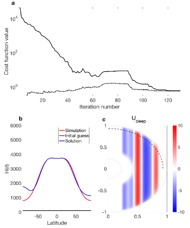
Figure 2: Model optimization for case A. (a) The reduction of the cost function (solid) and its contribution from the second term (dash-dotted), (b) Simulated, initial guess and solution for the depth of the surface wind (red, black, and blue, respectively), and (c) the solution for the deep flow (dashed line shows the section analyzed in Figs. 4b,d and 5b,d).

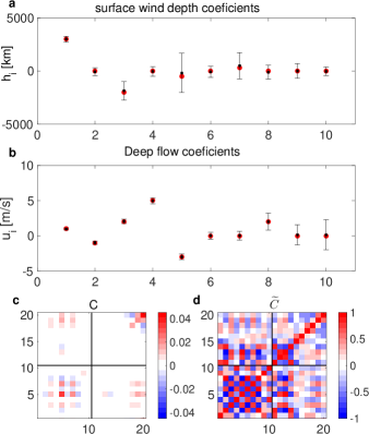
Figure 3: Model solution (black dots) and error standard deviation (error bars) for (a) The coefficients of the surface wind depth, and (b) the coefficients of the deep flow structure. Red dots are the simulation. (c) The error covariance matrix where entries 1-10 are for the coefficients defining the depth of the surface wind, and entries 11-20 are for the coefficients defining the structure of the deep flow. (d) The normalized error covariance matrix showing the correlation between the variables.

Next, we examine the solution for the control variables and the uncertainty associated with them. Similar to the solution presented in Fig. 2, the solution for the surface wind depth coefficients (Fig. 3a, black dots) and deep flow coefficients (Fig. 3b, black dots) are very close to the those used in the simulation (red dots). Using the error covariance matrix (Fig. 3c) we can calculate the standard deviation for each variable, taking the square root of the diagonal terms and renormalizing each variable. These uncertainties are shown as error bars in Fig. 3a,b. It is apparent that the uncertainties depend strongly on the variables, with some coefficients having small values and other much larger values. For example, the standard deviation of the errors associated with $h_{1}$ is $\sim 280$ km while that associated with $h_{5}$ is $\sim 2000$ km. The standard deviation of the errors associated with $A_{1}$ is $\sim 0.15$ m s^-1 while that associated with $A_{10}$ is $\sim 2$ m s^-1. Furthermore, there are strong correlations between the different variables (off diagonal terms in Fig. 3c), which need to be taken into account when estimating the actual uncertainty of the model solution. To illustrate this the normalized error covariance matrix

$$\tilde{C}_{i,j} = \frac{C_{i,j}}{\sqrt{C_{i,i}C_{j,j}}},$$

is shown in Fig. 3d. This matrix shows the correlation between the variables, so that the diagonal terms (self correlations) have a value of one, and off diagonal terms are the correlation between each two variables. It is clear that many strong positive and negative correlations exists, mainly between the coefficients defining the depth of the surface wind (indices 1-10), but also between these coefficients and those defining the structure of the deep flow (indices 11-20).

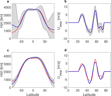
Figure 4: (a) Model solution for the depth of the surface wind (blue line), together with its uncertainties (shaded area) and the simulated wind depth (red line). (b) Same as (a), but for the deep flow structure along the radial distance of $0.93a$ (dashed line in Fig. 2c). Panels (c) and (d) are as (a) and (b), but for the case where the model is optimized with $N_{{\rm H}}=5$ and $N_{{\rm U}}=5$.

Given that complexity, interpreting the error covariance matrix in terms of the actual physical variables, the depth of the surface wind $H(\theta)$ and the deep flow $U_{{\rm deep}}$, requires that all information included in the covariance matrix is used. Following the methodology presented in section 2.5, we calculate the uncertainties associated with $H(\theta)$ and $U_{{\rm deep}}$. In Fig. 4a the standard deviation for the errors in the depth of the surface wind is shown as shading on top of the simulation. In the equatorial region, the model uncertainty is confined to a few hundred kilometers but at high latitudes the uncertainty rises to thousands of kilometers, implying that deviations in the observed gravitational moments on the order of $5\times 10^{-9}$ would results in the model inability to predict the depth of the surface wind over the high latitudes. The model solution for the deep flow structure along the radial distance of $0.93a\sim 65,000$ km (dashed line in Fig. 2c) shows (Fig. 4b) that while the deep flow is well constrained in the outer part of the planet (latitude $<30^{o}$), in the regions closer to the axis of rotation the uncertainty increases, yet its’ value is well below the magnitude of the solution there.

These results depend strongly on the number of optimized parameters; the more parameters are used, the larger the uncertainty is (Finocchiaro and Iess, 2010). To demonstrate this, consider a case where the model used for optimizing the solution is based on a simpler structure of surface wind depths, with $N_{{\rm H}}=5$, and a simpler deep wind structure, with $N_{{\rm U}}=5$ (Fig. 4c,d). While the uncertainty in the solution is now much smaller (shaded area), the solution itself (blue lines) is less exact, especially in the equatorial region. This illustrates the tradeoff between increasing the number of control variables (a more exact solution), and the associated increased uncertainty. In the specific case presented here, it is clear that for the deep flow structure $N_{{\rm U}}=5$ does not provide enough spatial variability since $A_{8}$ has a considerable contribution in the simulation (see Fig. 3b). The model solution (Fig. 4d, blue line) is missing a sizable part of the simulated flow structure (red line). The depth of the surface wind, on the other hand, has only little contribution from $h_{7}$, therefore the model solution with $N_{{\rm H}}=5$ (Fig. 4d, blue line) is quite similar to the simulated one (red line).

Finally, we discuss briefly a couple of modified experiments. First, a variant of the above experiment is to set the depth of the surface bound wind to be 10 times smaller, thus making it more superficial. Results show that it is more difficult to reconstruct the simulated depth of the surface wind, but overall the results are similar, especially for the deep flow. Uncertainties also are qualitatively similar. In another variation, in addition to the surface depth and the structure of the deep flow we also set as a control variable the depth for the deep flow. The ability to reach the global minimum is this case is degraded considerably and the solution depends on the initial guess. In some cases a global minimum is reached, but in others the solution is far from the simulation, not only in the depth of the deep flow, but also in all other parameters. As discussed below, this is a less of a problem in case B where the depth of the deep flow is restricted to relatively shallow levels.

3.1.2 Case B - restricted deep flow and shallow surface wind

Next, we examine the characteristics of the optimization where the simulated gravitational moments are based on case B, where the depth of the deep flow is much more limited, and where the surface wind is shallow (section 2.3, Fig. 1d,e,f).

As in case A, the control variables include the 10 surface wind depth coefficients and the 10 deep flow coefficients. Later on, we also consider the depth of the deep flow $a_{D}$ as a control variable. Starting with an initial guesses similar to those used in section 3.1.1, the optimization is able to reach a solution that is in general as good as the one achieved for the experiment presented in section 3.1.1 (Fig. 5). The solution reproduces well the depth of the surface wind aside from the polar regions (panel a) and the deep flow (panel b). Restricting the number of surface wind depth coefficients and deep flow structure coefficients to 5 (panels c,d), reduces the uncertainties but causes the solution to agree less with the simulation.

Several important differences from case A arise. First, comparing Fig. 4 and Fig. 5, while the uncertainties for the deep flow are similar in both cases, the uncertainties for the depth of the surface wind are larger in case B. This is true for both large or small number of coefficients used (panels a and c). More importantly, since the depth of the surface wind is now 10 times shallower, the even larger magnitude of the uncertainties implies that aside from the equatorial region, it would be impossible to place a lower limit on the depth (the gray zone reaches a depth of zero), and the upper limit is now more than $1000$ km in most latitudes (panel a). Even with the reduction of the number of coefficients (panel c), the uncertainty is still much larger than the simulated depth.

On the other hand, including the optimization of the deep flow depth $a_{{\rm D}}$ is now feasible in some cases. While in the equivalent experiments discussed in section 3.1.1, in inclusion of $a_{{\rm D}}$ resulted in a solution dependent on the initial guess of the control variables, in case B a global solution very similar to the one shown in Fig. 5 could be reached when the initial guess is $a_{{\rm D}}\gtrsim 50,000$ km (not shown). With that, setting the initial guess to lower values results in the optimization reaching a local minimum that is far from the simulated one.

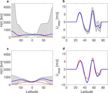
Figure 5: Results for case B - (a) Model solution for the depth of the surface wind (blue line), together with its uncertainties (shaded area) and the simulated wind depth (red line. (b) Same as (a), but for the deep flow structure along the radial distance of $0.93a$ (dashed line in Fig. 2c). Panels (c) and (d) are as (a) and (b), but for the case where the model is optimized with $N_{{\rm H}}=5$ and $N_{{\rm U}}=5$.

3.2 Optimization with unconstrained deep flow

So far, the same model has been used for generating the simulation and to search for the solution. We now examine a case where the model used for finding the solution differs profoundly from the one used to simulate the observations. An extreme test for the model ability to reach a solution would be to relax the structure of the deep flow, from cylinders to a general flow that has absolutely no restrictions in both latitude and depth. Physically such a solution is likely unjustifiable, but this serves as a good test for the model’s ability to reach a solution without any constraints. The implication to the adjoint model and optimization process is profound. Now, in addition to the 10 control variables of the depth of the surface wind, there are $N_{\theta}\times N_{r}$ control variables of $U_{{\rm deep}}$ (compared to the 10 control variables used before to set the deep wind structure). While in the above experiments we set $N_{\theta}=361$ and $N_{r}=174$ ($0.5$ deg resolution in latitude and 10 vertical levels per scale height), here a reduced resolution has to be employed, $N_{\theta}=91$ and $N_{r}=87$, so that the total length of the control variable is $91\times 87+10=7927$. Even with such a reduced resolution, the numerical calculation of the optimization (finding the search direction and step length at each iteration, see Galanti and Kaspi (2016) for details) requires considerable computational resources. Note that since we are producing the ’observations’ and looking for the solution with the same model resolution, reducing the resolution is self-consistent and does not affect the results. However, when analyzing the Juno observations, numerical capability to solve the high resolution version would have to be developed.

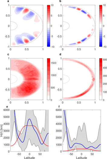
Figure 6: Looking for an optimized solution with the unconstrained deep flow, in both case A (left panels), and case B (right panels). Shown are the solution for the deep flows (a,b), the uncertainties associated with this solution (c,d), and the solution for the depth of the surface wind (e,f) with its uncertainties.

We consider here our ability to reach the solution in both simulations, case A and case B (Fig. 6). A striking characteristic of the solution in both cases (Fig. 6a,b) is the structure of the deep flow is aligned mostly in the radial direction. Now that the deep flow is no longer constrained to flow parallel to the axis of rotation, it is the thermal wind balance and the radial independence of the gravitational moments that set the optimal flow. That said, it is encouraging that the overall structure is similar to the simulated one (Fig. 1b,d). Going from the poles to the equator, the pattern of negative, positive, negative, and then positive flow, is apparent in both cases. The solution in both cases also identifies the lack of deep flow close to the equator. The depth of the deep flow, however, has different characteristics in the two cases. In case A (Fig. 6a), the deep flow is not extending all the way to a depth of $30,000$ km as in the simulation, suggesting the the flow in that region (if existing) could not be recovered in the model solution. This results form the fact that the affect of the density on the gravitational moments is decreasing with depth. In case B (Fig. 6b), the solution extends in the entire region where the deep flow exists in the simulation.

The major limitation however comes from the uncertainties (Fig. 6b,d), which extend over the entire region and have unphysical values of more than $1,500\,{\rm m\,s^{-1}}$ in case A, and more than $500$ m s^-1 in case B. This is also the case for the uncertainties in the solution for the depth of the surface wind (Fig. 6e,f), which is of the order of several thousands of kilometers.

4 Conclusion

We develop a methodology to examine the upcoming high accuracy gravity measurements by the Juno spacecraft. We allow the flow structure to be as general as possible, with a deep flow which is completely decoupled from a surface bound observed flow. The model is composed from a forward dynamical model that relates the 3D flow to the density and gravity fields, and an inverse model that, given the observed gravity field, can trace back the complex flow.

In order to simulate possible observations of the gravity field, we constructed two observational scenarios. In the first, the interior flow is deep, and the cloud-level flow penetrates to a depth of $3000$ km. Deeper flows in this case have a comparable effect on the gravitational moments. In the second scenario, interior flow is confined to a relatively narrow region, and the surface bound flow is shallow, penetrating to a depth of only $300$ km. The gravitational moments in this case are mostly affected by the deep flow, while the surface bound flow has a negligible effect. These two cases were selected as representative cases to allow examination of substantially different scenarios.

We examine the inverse model ability to reach a solution for both scenarios. We start from an initial guess of no interior flow, and close to zero depth of the surface bound flow. We then seek for a solution that minimize the difference between the calculated and the simulated gravity moments. For both simulations, case A and case B, the optimized solution reproduces well the depth of the surface wind (aside from the polar regions) and the deep flow structure and amplitude. In both cases, optimizing when the number of surface wind depth coefficients and deep flow structure coefficients is restricted to 5, caused the uncertainties in the solution to be reduced, but the solution agreed less with the simulation. Nonetheless, several differences between the cases exist. The uncertainties for the depth of the surface wind are larger in case B. This is true for both large or small number of coefficients used. More importantly, since the depth of the surface wind in case B is 10 times shallower than case A, even larger magnitude of the uncertainties implies that aside from the equatorial region, it would be impossible to place a lower limit on the depth. Overall, in a case where the surface bound flow is on the order of $\sim 100$ km, and there exist a decoupled flow in the interior, it will be very difficult to estimate the depth of surface flow. Even with the reduction of the number of coefficients, the uncertainty is still much larger than the simulated depth.

Finally, we examined a case where the model used for finding the solution differs considerably from the one used to simulate the observations. We tested the model ability to reach a solution when the flow field is free to have any possible form, so it is not restricted to cylindrical shapes, and can have a general flow that has absolutely no restrictions in both latitude and depth. Physically, it is hard to justify such a solution, but this serves as a good test for the model’s ability to reach a solution without any constraints. In both simulations, case A and case B, the structure of the solution was aligned mostly in the radial direction and not parallel to the axis of rotation as the simulated flow. Nevertheless, the overall structure of the solutions was similar to the simulated one. The depth of the deep flow did not match well the simulated one, and had different characteristics in the two cases. A major limitation comes from the uncertainties that extend over the entire region and have unphysical values This was also the case for the uncertainties associated with the solution for the depth of the surface wind. Their values was in the order of several thousands of kilometers.

The novelty of the adjoint based inverse method presented here is in the ability to identify complex flow dynamics given the expected Juno measurements of gravity moments. Unlike any previous studies, this model allows also for the existence of deep cylindrical flows that have no manifestation in the observed cloud-level wind. Furthermore, the flexibility of the adjoint method allows for a wide range of dynamical setups, so that when new observations and physical understanding will arise, these constraints could be easily implemented and used to better decipher Jupiter flow dynamics.

Acknowledgments: We thank Eli Tziperman and the members of the Juno science team interiors working group for helpful discussions. This research has been supported by the Israeli Ministry of Science and the Minerva foundation with funding from the Federal German Ministry of Education and Research. We also acknowledge support from the Helen Kimmel Center for Planetary Science at the Weizmann Institute of Science.

References

- Atkinson et al. (1996) Atkinson, D. H., Pollack, J. B., Seiff, A., May 1996. Galileo doppler measurements of the deep zonal winds at Jupiter. Science 272, 842–843.
- Aurnou and Olson (2001) Aurnou, J. M., Olson, P. L., 2001. Strong zonal winds from thermal convectionin a rotating spherical shell. Geophys. Res. Lett. 28 (13), 2557–2559.
- Bolton (2005) Bolton, S. J., March 2005. Juno final concept study report. Tech. Rep. AO-03-OSS-03, New Frontiers, NASA.
- Busse (1976) Busse, F. H., 1976. A simple model of convection in the Jovian atmosphere. Icarus 29, 255–260.
- Busse (1994) Busse, F. H., 1994. Convection driven zonal flows and vortices in the major planets. Chaos 4 (2), 123–134.
- Chan and Mayr (2013) Chan, K. L., Mayr, H. G., Jun. 2013. Numerical simulation of convectively generated vortices: Application to the Jovian planets. Earth Planet. Sci. Lett. 371, 212–219.
- Cho and Polvani (1996) Cho, J., Polvani, L. M., 1996. The formation of jets and vortices from freely-evolving shallow water turbulence on the surface of a sphere. Phys. of Fluids. 8, 1531–1552.
- Christensen (2002) Christensen, U. R., 2002. Zonal flow driven by strongly supercritical convection in rotating spherical shells. J. Fluid Mech. 470, 115–133.
- Conrath et al. (1981) Conrath, B. J., Flasar, F. M., Pirraglia, J. A., Gierasch, P. J., Hunt, G. E., Sep. 1981. Thermal structure and dynamics of the Jovian atmosphere. ii - visible cloud features. J. Geophys. Res. 86, 8769–8775.
- Dowling and Ingersoll (1988) Dowling, T. E., Ingersoll, A. P., 1988. Potential vorticity and layer thickness variations in the flow around Jupiter’s great red spot and white oval BC. J. Atmos. Sci. 45 (8), 1380–1396.
- Dowling and Ingersoll (1989) Dowling, T. E., Ingersoll, A. P., 1989. Jupiter’s great red spot as a shallow water system. J. Atmos. Sci. 46 (21), 3256–3278.
- Finocchiaro and Iess (2010) Finocchiaro, S., Iess, L., 2010. Numerical simulations of the gravity science experiment of the Juno mission to Jupiter. In: Spaceflight mechanics. Vol. 136. Amer. Astro. Soc., pp. 1417–1426.
- Galanti and Kaspi (2016) Galanti, E., Kaspi, Y., 2016. An adjoint-based method for the inversion of the juno and cassini gravity measurements into wind fields. Astrophys. J. 820 (2), 91.
- Galanti et al. (2016) Galanti, E., Kaspi, Y., Tziperman, E., 2016. A full, self-consistent, treatment of thermal wind balance on fluid planets. J. Fluid Mech.In revision.
- Gastine and Wicht (2012) Gastine, T., Wicht, J., May 2012. Effects of compressibility on driving zonal flow in gas giants. Icarus 219, 428–442.
- Gastine et al. (2013) Gastine, T., Wicht, J., Aurnou, J. M., Jul. 2013. Zonal flow regimes in rotating anelastic spherical shells: An application to giant planets. Icarus 225, 156–172.
- Gierasch et al. (1986) Gierasch, P. J., Magalhaes, J. A., Conrath, B. J., Sep. 1986. Zonal mean properties of Jupiter’s upper troposphere from Voyager infrared observations. Icarus 67, 456–483.
- Heimpel et al. (2005) Heimpel, M., Aurnou, J., Wicht, J., Nov 2005. Simulation of equatorial and high-latitude jets on Jupiter in a deep convection model. Nature 438, 193–196.
- Heimpel and Gómez Pérez (2011) Heimpel, M., Gómez Pérez, N., 2011. On the relationship between zonal jets and dynamo action in giant planets. Geophys. Res. Lett. 38 (14).
- Hubbard (1999) Hubbard, W. B., Feb. 1999. Note: Gravitational signature of Jupiter’s deep zonal flows. Icarus 137, 357–359.
- Jones and Kuzanyan (2009) Jones, C. A., Kuzanyan, K. M., Nov. 2009. Compressible convection in the deep atmospheres of giant planets. Icarus 204, 227–238.
- Kaspi (2013) Kaspi, Y., Feb. 2013. Inferring the depth of the zonal jets on Jupiter and Saturn from odd gravity harmonics. Geophys. Res. Lett. 40, 676–680.
- Kaspi et al. (2016) Kaspi, Y., Davighi, J. E., Galanti, E., Hubbard, W. B., 2016. The gravitational signature of internal flows in giant planets: comparing the thermal wind approach with barotropic potential-surface methods. Icarus 276, 170–181.
- Kaspi and Flierl (2007) Kaspi, Y., Flierl, G. R., 2007. Formation of jets by baroclinic instability on gas planet atmospheres. J. Atmos. Sci. 64, 3177–3194.
- Kaspi et al. (2009) Kaspi, Y., Flierl, G. R., Showman, A. P., 2009. The deep wind structure of the giant planets: Results from an anelastic general circulation model. Icarus 202, 525–542.
- Kaspi et al. (2010) Kaspi, Y., Hubbard, W. B., Showman, A. P., Flierl, G. R., Jan. 2010. Gravitational signature of Jupiter’s internal dynamics. Geophys. Res. Lett. 37, L01204.
- Kong et al. (2016) Kong, D., Zhang, K., Schubert, G., 2016. Odd gravitational harmonics of jupiter: Effects of spherical versus nonspherical geometry and mathematical smoothing of the equatorially antisymmetric zonal winds across the equatorial plane. Icarus 277, 416 – 423.
- Lian and Showman (2010) Lian, Y., Showman, A. P., May 2010. Generation of equatorial jets by large-scale latent heating on the giant planets. Icarus 207, 373–393.
- Liu and Schneider (2010) Liu, J., Schneider, T., 2010. Mechanisms of jet formation on the giant planets. J. Atmos. Sci. 67, 3652–3672.
- Orton et al. (1998) Orton, G. S., Fisher, B. M., Baines, K. H., Stewart, S. T., Friedson, A. J., Ortiz, J. L., Marinova, M., Ressler, M., Dayal, A., Hoffmann, W., Hora, J., Hinkley, S., Krishnan, V., Masanovic, M., Tesic, J., Tziolas, A., Parija, K. C., Sep. 1998. Characteristics of the Galileo probe entry site from earth-based remote sensing observations. J. Geophys. Res. 103, 22791–22814.
- Pedlosky (1987) Pedlosky, J., 1987. Geophysical Fluid Dynamics. Spinger.
- Porco et al. (2003) Porco, C. C., West, R. A., McEwen, A., Del Genio, A. D., Ingersoll, A. P., Thomas, P., Squyres, S., Dones, L., Murray, C. D., Johnson, T. V., Burns, J. A., Brahic, A., Neukum, G., Veverka, J., Barbara, J. M., Denk, T., Evans, M., Ferrier, J. J., Geissler, P., Helfenstein, P., Roatsch, T., Throop, H., Tiscareno, M., Vasavada, A. R., 2003. Cassini imaging of Jupiter’s atmosphere, satellites and rings. Science 299, 1541–1547.
- Rhines (1975) Rhines, P. B., 1975. Waves and turbulence on a beta plane. J. Fluid Mech. 69, 417–443.
- Rhines (1979) Rhines, P. B., 1979. Geostrophic turbulence. Ann. Rev. Fluid Mech. 11, 401–441.
- Scott and Polvani (2007) Scott, R. K., Polvani, L. M., 2007. Forced-dissipative shallow-water turbulence on the sphere and the atmospheric circulation of the giant planets. J. Atmos. Sci. 64, 3158–3176.
- Showman (2007) Showman, A. P., 2007. Numerical simulations of forced shallow-water turbulence: effects of moist convection on the large-scale circulation of Jupiter and Saturn. J. Atmos. Sci. 64, 3132–3157.
- Showman and Dowling (2000) Showman, A. P., Dowling, T. E., Sep. 2000. Nonlinear simulations of Jupiter’s 5-micron hot spots. Science 289, 1737–1740.
- Wicht et al. (2002) Wicht, J., Jones, C. A., Zhang, K., Feb. 2002. Instability of zonal flows in rotating spherical shells: An application to Jupiter. Icarus 155, 425–435.
- Williams (1978) Williams, G. P., 1978. Planetary circulations: 1. barotropic representation of the Jovian and terrestrial turbulence. J. Atmos. Sci. 35, 1399–1426.
- Williams (2003) Williams, G. P., 2003. Jovian dynamics. part 3: Multiple, migrating and equatorial jets. J. Atmos. Sci. 60, 1270–1296.
- Zhang et al. (2015) Zhang, K., Kong, D., Schubert, G., JUN 20 2015. Thermal-gravitational wind equation for the wind-induced gravitational signature of giant gaseous planets: mathematical derivation, numerical method, and illustrative solutions. Astrophys. J. 806 (2).