Multifactor CES General Equilibrium: Models and Applications

Abstract

Sector specific multifactor CES elasticities of substitution and the corresponding productivity growths are jointly measured by regressing the growths of factor-wise cost shares against the growths of factor prices. We use linked input-output tables for Japan and the Republic of Korea as the data source for factor price and cost shares in two temporally distant states. We then construct a multi-sectoral general equilibrium model using the system of estimated CES unit cost functions, and evaluate the economy-wide propagation of an exogenous productivity stimuli, in terms of welfare. Further, we examine the differences between models based on a priori elasticities such as Leontief and Cobb-Douglas.

-0.15

1 Introduction

In this study, we measure the multifactor CES elasticity of substitution, jointly with the productivity growth, for multiple industrial sectors, by way of two temporally distant cross-sectional data (i.e., linked input–output tables). As we learn the multifactor CES unit cost function, we discover that an industry specific elasticity can be estimated by regressing the growth of factor-wise cost shares against the growth of factor-wise prices. We also discover that the industry specific productivity growth can be measured via the intercept of the regression line. Consequently, we make use of the linked input–output tables in order to observe the cost shares and the price changes spanning over two periods for multiple industrial sectors.

The two-input constant elasticity of substitution (CES) function was first introduced by Arrow et al. [1961], and Uzawa [1962] and McFadden [1963] later showed that elasticities were still unique for the case of more than two factor inputs. Empirical analyses concerning the measurement of CES elasticities [e.g., McKibbin and Wilcoxen, 1999, van der Werf, 2008, Koesler and Schymura, 2015] have been based upon time series data, while embedding nest structures into the two-input CES framework conforming to the work by Sato [1967], to handle elasticities between more than two factors of production. The number of factors and thus of estimable elasticities, can nevertheless be narrowed depending on the availability of time series data. Since we are interested in constructing a multisector general equilibrium model that calls for multifactor production functions, we take the advantage of an alternative approach, exploiting cross-sectional data.

When a multisectoral general equilibrium model is established, assessments can be made of the arbitrary productivity shock resulting from technological innovation, in terms of welfare gained. Previous studies in this regard have assumed a constant and uniform unit elasticity [Klein, 1952–1953], or have used empirically estimated elasticities in Translog or multistage (nested) CES functions with a highly aggregated and thus limited number of substitutable factors. Examples include works by Kuroda et al. [1984], Saito and Tokutsu [1989], and Tokutsu [1994], and many of the works concerning CGE models such as studies by Böhringer et al. [2015] and Go et al. [2016]. In contrast, our approach allows us to construct an empirical model of multifactor production with different elasticities of substitution among many (over 350) industrial sectors. Moreover, this approach allows us to prospectively portray the ex post technological structure following any given exogenous productivity shock and to account for welfare in terms of economy-wide input–output performances.

We measure the welfare changes attributed to the exogenous productivity change by SCS (social cost saved), i.e., the difference in the total primary factor inputs required to net produce a fixed amount of final consumption, given the productivity change. We find in theory that SCS will be positive (primary factor inputs will always be saved) in every sector if the exogenous productivity is improving, and vice-versa, under the system with uniform CES elasticity less than unity which is inclusive of Cobb–Douglas and Leontief systems. Hence conversely, such a law may not necessarily hold for the case of CES system with non-uniform elasticities; and this is verified by the empirical analysis of SCS using the estimated multifactor CES system.

The remainder of this paper is organized as follows. In the next section, we introduce the basics of multifactor CES elasticity and productivity growth estimation and apply the protocol to linked input–output tables for Japan and the Republic of Korea having sufficient capacity as far as degrees of freedom of the regression. In Section 3, we replicate the current technological structure as the general equilibrium state of a system of empirically estimated multifactor CES functions; further, we trace out how that structure is transformed by exogenous productivity stimuli. Section 4 provides concluding remarks.

2 The Model

2.1 Multifactor CES Functions

A constant-returns multifactor CES production function of an industrial sector (index $j$ omitted) has the following form:

$$y=zf\left(\mathbf{x}\right)=z\left(\sum_{i=0}^{n}{{\lambda}}_{i}^{\frac{1}{\sigma}}x_{i}^{\frac{\sigma-1}{\sigma}}\right)^{\frac{\sigma}{\sigma-1}}$$

where, $y$ denotes the output and $x_{i}$ denotes the $i$th factor input. Here, the share parameters are assumed to maintain ${\lambda}_{i}>0$ and $\sum_{i}{\lambda}_{i}=1$, while the elasticity of substitution $\sigma\geq 0$ is subject to estimation. Also, we are interested in measuring the growth of productivity i.e., $\Delta\ln z$, where $\Delta$ represents temporally distant differences.

Displayed below is the unit cost function compatible with the multifactor CES production function:

$$c=z^{-1}h\left(\mathbf{w}\right)=\frac{1}{z}\left(\sum_{i=0}^{n}{\lambda}_{i}w_{i}^{\gamma}\right)^{{1}/{\gamma}}$$

where, $c$ denotes the unit cost of the output, and $w_{i}$ denotes the $i$th factor price. Here, we use $\gamma=1-\sigma$ for convenience. The cost share of the $i$th input $a_{i}$ can be determined, in regard to Shephard’s lemma, by differentiating the unit cost function:

$${a}_{i}=\frac{\partial c}{\partial w_{i}}\frac{w_{i}}{c}={\lambda}_{i}\left(zc/w_{i}\right)^{-\gamma}$$ (1)

By taking the log of both sides, we have

$$\ln{a}_{i}=\ln{\lambda}_{i}-\gamma\ln z+\gamma\ln\left(w_{i}/c\right)$$

As we observe two temporally distant values for cost shares ($a_{i}^{0}$ and $a_{i}^{0}$), factor prices ($w_{i}^{0}$ and $w_{i}^{1}$), and unit costs of outputs as prices ($c^{0}=w^{0}$ and $c^{1}=w^{1}$) reflecting perfect competition, we find two identities regarding the data:

$$\ln{a}^{0}_{i} =\ln{\lambda}_{i}-\gamma\ln z^{0}+\gamma\ln\left(w^{0}_{i}/w^{0}\right)+\epsilon_{i}^{0}$$

$$\ln{a}^{1}_{i} =\ln{\lambda}_{i}-\gamma\ln z^{1}+\gamma\ln\left(w^{1}_{i}/w^{1}\right)+\epsilon_{i}^{1}$$

where, we assume that $\epsilon_{i}^{0}$ and $\epsilon_{i}^{1}$ are identically and normally distributed disturbance terms. Subtraction results in the main regression equation of the following:

$$\Delta\ln{a}_{i}=-\gamma\Delta\ln z+\gamma\Delta\ln\left(w_{i}/w\right)+\epsilon_{i}$$ (2)

Here, the disturbance term $\epsilon_{i}=\epsilon_{i}^{0}-\epsilon_{i}^{1}$ is identically normally distributed, so that one can estimate $\gamma$ and $\Delta\ln z$ via a simple linear regression (2). That is, by regressing the growth of factor-wise cost shares i.e, $\Delta\ln{a}_{i}$ on the growth of relative prices i.e., $\Delta\ln\left(w_{i}/w\right)$, the slope gives the estimate of $\gamma$ while the intercept gives the estimate of $-\gamma\Delta\ln z$. Also, note that ${\lambda}_{i}$ can be calibrated via (1) as long as we have the estimate for $\gamma$.

2.2 The Data and Estimation

A set of linked input–output tables includes sectoral transactions in both nominal and real terms. Since real value is adjusted for inflation, in order to enable comparison of quantities as if prices had not changed, and since nominal value is not adjusted, we use a price index to convert nominal into real values. That is, if we standardize the value of a commodity at the reference state as real, its nominal (unadjusted) value at the target state relative to the reference state equals the price index called a deflator. Naturally, the 1995–2000–2005 linked input–output tables for both Japan [MIAC, 2011] and Korea [BOK, 2015] include factor-wise deflators (395 factors for Japan and 350 factors for Korea) spanning the fiscal years recorded. These linked input–output tables, however, do not include deflators for primary factor (i.e., labor and capital) and therefore, we used the quality-adjusted price indexes compiled by JIP [2015] for Japan and by KIP [2015] for Korea in order to inflate the primary factor inputs observed in nominal values.

Hence, observations for both the dependent variables (cost shares as input–output coefficients $a_{ij}$) and the independent variables (price ratios $w_{j}/w_{i}$) for estimating (2) become available with sufficient capacity, in terms of degrees of freedom, as we verify that there are $n+1$ inputs: namely, $i=0,1,\cdots,n$; and $n$ outputs, namely $j=1,\cdots,n$, for an input–output table. In particular, we use the 2000 and 2005 input–output coefficient matrices out of the three-period linked input–output tables as the data for the cost share growth (i.e., $\Delta\ln a_{ij}$) and as we set the reference state at year 2000, the five-year growth of output-relative factor prices becomes simply the log difference between deflators; that is,

$$\Delta\ln w_{i}/w_{j}=\ln p_{i}/p_{j}$$

where $p_{i}$ denotes the deflator for commodity $i$ in year 2005 with respect to year 2000.

Figure 2 displays the estimated CES elasticity (i.e., $\sigma_{j}=1-\gamma_{j}$) with respect to the statistical significance of $\gamma_{j}$ i.e., the slope of the regression equation (2) in terms of P-value, for Japan. Figure 2 is the version for Korea. Note that CES elasticities were statistically significant (P-value $<0.1$) for 176 out of 395 sectors for Japan, whereas 166 sectors were significant out of 350 sectors for Korea. The results of estimation are summarized in the Appendix, Tables Appendix and Appendix for Japan and Korea, respectively. These tables are confined to sectors whose slopes ($\gamma_{j}=1-\sigma_{j}$) of the regression (2) are statistically significant, and we indicate the level of significance by *** (0.01 level), **(0.05 level), and *(0.1 level), along with the estimated elasticities.

Figure 1: CES elasticity vs significance (Japan)

Figure 2: CES elasticity vs significance (Korea)

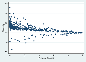
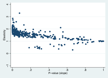
Note that we accept the null (i.e., $\gamma_{j}=1-\sigma_{j}=0$) for sectors with statistically insignificant slope, and in that event, the average of elasticities i.e., $\sum_{j=1}^{n}\sigma_{j}/n$ was $1.32$ for Japan and $1.39$ for Korea. Alternatively, if we accept all the estimates of elasticities, regardless of statistical significances, the average of elasticities was $1.46$ for Japan and $1.52$ for Korea.

These multifactor CES elasticities are comparable to other estimates in the literature. The GTAP [2016] substitution elasticities for intermediate inputs which are broadly employed in CGE studies [e.g., Álvarez-Martínez and Polo, 2012, Antimiani et al., 2015] range from 0.20 to 1.68, while those among internationally traded goods (i.e., Armington elasticities) are generally larger ranging from 1.15 to 34.40, depending on the industrial sector. Welsch [2006]’s estimate for mean Armington elasticities ranges from negative 2.06 to positive 2.17, also depending on the industrial sector. Note that these estimates are fairly comparable to the Koesler and Schymura [2015]’s KLEM nest-wise CES elasticity estimates for 36 industrial sectors.

In the third column of Tables Appendix and Appendix, we display the productivity growth $\Delta\ln z$, labeled as TFPg (Total Factor Productivity growth), which is the estimated constant of (2) divided by the negative of the corresponding slope. Accordingly, the statistical significances of TFPg are evaluated by way of bootstrapping (with 400 replications) on the basis of regression (2). The statistical significances of the underlying intercept are indicated with parenthesis. Note also that these tables are sorted by the level of the estimated TFPg. Let us now make some assessments of the estimated TFPg in regard to other possible productivity measurements. Below is the log of Törnqvist index

$$\text{TFPg (Translog)}=-\ln p+\sum_{i=0}^{n}\left(\frac{a_{i}^{0}+a_{i}^{1}}{2}\right)\ln p_{i}$$ (3)

the exactness of which Diewert [1976] showed in measuring the productivity growth of Translog functions. Thus, we know that (3) is equal to the productivity growth of the underlying Translog function with or without knowing its parameters. Note that although it is almost impossible to estimate the parameters of a Translog function with one hundred factor inputs, its productivity growth can be measured using the same data (cost shares and price changes) as we use in estimating productivity for a multifactor CES function. Star and Hall [1976] showed that the Törnqvist index is a good approximation of TFPg measurement irrespective of the type of aggregator function and the interval of observations.

Figure 3: TFPg of different measurements. (Japan)

Figure 4: TFPg of different measurements. (Korea)

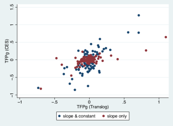
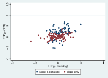
In Figures 4 and 4, we plot the estimated TFPg for a multifactor CES function, tagged as TFPg (CES) for all sectors listed in Tables Appendix and Appendix, against the log of the Törnqvist indexes, tagged as TFPg (Translog). Blue dots indicate sectors whose slope and intercept of regression (2) were both statistically significant (P-value $<0.1$), whereas red dots indicate sectors with a slope that was significant but an intercept that was not. In both cases, we observe agreements between the two TFPg measurements; therefore, we evaluate them objectively as summarized in Table 1. Here, Correlation designates Pearson’s correlation coefficient, whereas Concordance designates Lin [2000]’s concordance correlation coefficient. Note that “Slope Only” significant sectors are of red dots, and “Sope and Constant” significant sectors are of blue dots, in Figures 4 and 4; and “Slope” indicates all slope significant sectors, thus, union of red and blue sectors. “Bootstrapping” indicates sectors with significant TFPg (CES) estimates via bootstrapping. To say this in other words, by way of multifactor CES function, we obtain TFPg estimates similar to those based on Translog functions that are very general in terms of elasticities of substitution set aside their estimability, and yet, a multifactoral elasticity of substitution is estimable over very many factor inputs. Note however that in the event that we accept the null for the insignificant slope of the regression (2), we must assume that the function is Cobb–Douglas and that TFPg is unmeasureable.

Table 1: Concordances and correlations between Translog and multifactor CES TFPg estimates.

Sectors	Concor.	Correl.	Obs.
Slope (JPN)	$0.645$	$0.669$	176
Slope Only (JPN)	$0.673$	$0.707$	100
Slope and Constant (JPN)	$0.633$	$0.741$	76
Bootstrapping (JPN)	$0.794$	$0.889$	21
Slope (KOR)	$0.305$	$0.413$	166
Slope Only (KOR)	$0.309$	$0.340$	97
Slope and Constant (KOR)	$0.370$	$0.413$	69
Bootstrapping (KOR)	$0.623$	$0.707$	33

3 Prospective Analysis

3.1 Projected Prices

In the following section, we construct a multisectoral general equilibrium model that reflects all measured elasticities and observed current cost shares; further, we exogenously impose some productivity change into the model and simulate the multisectoral propagation that can potentially take place. For sake of simplicity, let us normalize all current prices at unity. In that event, we know by (1) that:

$$a_{ij}={\lambda}_{ij},~{}~{}~{}~{}~{}~{}\sum_{i=0}^{n}{a_{ij}}=1,~{}~{}~{}~{}j=1,2,\cdots,n$$

Then, the system of CES unit cost functions in equilibrium, under some exogenously given productivity change i.e., $\mathbf{z}=\left(z_{1},z_{2},\cdots,z_{n}\right)\neq\boldsymbol{1}$, must be in the following state:

$$\begin{split}\pi_{1}&=z_{1}^{-1}\left(a_{01}\pi_{0}^{{\gamma}_{1}}+a_{11}\pi_{1}^{{\gamma}_{1}}+\cdots a_{n1}\pi_{n}^{{\gamma}_{1}}\right)^{\frac{1}{{\gamma}_{1}}}\\ \pi_{2}&=z_{2}^{-1}\left(a_{02}\pi_{0}^{{\gamma}_{2}}+a_{12}\pi_{1}^{{\gamma}_{2}}+\cdots a_{n2}\pi_{n}^{{\gamma}_{2}}\right)^{\frac{1}{{\gamma}_{2}}}\\ &\vdots\\ \pi_{n}&=z_{n}^{-1}\left(a_{0n}\pi_{0}^{{\gamma}_{n}}+a_{1n}\pi_{1}^{{\gamma}_{n}}+\cdots a_{nn}\pi_{n}^{{\gamma}_{n}}\right)^{\frac{1}{{\gamma}_{n}}}\end{split}$$ (4)

where the projected (ex post) general equilibrium price for factor $i$ is denoted by $\pi_{i}$. Note that the current state i.e, $\mathbf{z}=\boldsymbol{1}$ can be reproduced by setting all prices at the current state i.e., $\boldsymbol{\pi}=\boldsymbol{1}$ and vice versa.

The projected price, ex post the exogenous productivity change, can be obtained by solving (4) for $\boldsymbol{\pi}$. By rearranging, we have:

$$z_{1}^{{\gamma}_{1}}\pi_{1}^{{\gamma}_{1}} =a_{01}\pi_{0}^{{\gamma}_{1}}+a_{11}\pi_{1}^{{\gamma}_{1}}+\cdots a_{n1}\pi_{n}^{{\gamma}_{1}}$$

$$z_{2}^{{\gamma}_{2}}\pi_{2}^{{\gamma}_{2}} =a_{02}\pi_{0}^{{\gamma}_{2}}+a_{12}\pi_{1}^{{\gamma}_{2}}+\cdots a_{n2}\pi_{n}^{{\gamma}_{2}}$$

$$\vdots$$

$$z_{n}^{{\gamma}_{n}}\pi_{n}^{{\gamma}_{n}} =a_{0n}\pi_{0}^{{\gamma}_{n}}+a_{1n}\pi_{1}^{{\gamma}_{n}}+\cdots a_{nn}\pi_{n}^{{\gamma}_{n}}$$

or by way of row vectors and matrices:

$$\boldsymbol{\pi}^{\boldsymbol{\gamma}}\left<\mathbf{z}^{\boldsymbol{\gamma}}\right>=\mathbf{a}_{0}+\boldsymbol{\pi}^{\boldsymbol{\gamma}}\mathbf{A}$$

where $\boldsymbol{\pi}^{\boldsymbol{\gamma}}=\left(\pi_{1}^{\gamma_{1}},\cdots,\pi_{n}^{\gamma_{n}}\right)$ and $\mathbf{z}^{\boldsymbol{\gamma}}=\left(z_{1}^{\gamma_{1}},\cdots,z_{n}^{\gamma_{n}}\right)$, while we set the price of a primary input as a numéraire i.e., $\pi_{0}=1$. Angle brackets indicate diagonalization. Note that $\mathbf{A}$ and $\mathbf{a}_{0}$ are the current input–output coefficients matrix and value added coefficients vector, respectively. Now, the projected equilibrium price $\boldsymbol{\pi}$ can be obtained in terms of $\mathbf{z}$:

$$\boldsymbol{\pi}=\left(\mathbf{a}_{0}\left[\left<\mathbf{z}^{\boldsymbol{\gamma}}\right>-\mathbf{A}\right]^{-1}\right)^{\frac{1}{\boldsymbol{\gamma}}}$$ (5)

Besides CES, we may use (5) to obtain the projected price for the cases of Leontief ($\boldsymbol{\gamma}=\mathbf{1}$) and Cobb–Douglas ($\boldsymbol{\gamma}=\mathbf{0}$). The Leontief case is straightforward:

$$\boldsymbol{\pi}=\mathbf{a}_{0}\left[\left<\mathbf{z}\right>-\mathbf{A}\right]^{-1}$$ (6)

For the Cobb–Douglas case, we first take the log of (4) and then let $\boldsymbol{\gamma}\to\mathbf{0}$. Below, we work on the unit cost function of any industrial sector $j$ while omitting the subscript:

$$\ln\pi+\ln z=\frac{\ln\left(a_{0}+\sum_{i=1}^{n}a_{i}\pi_{i}^{\gamma}\right)}{\gamma}\to\sum_{i=1}^{n}a_{i}\ln\pi_{i}$$

Here, we applied l’Hospital’s rule when we let $\gamma\to 0$, since in that event the nominator and the denominator both approach zero. By way of row vectors and matrices, this can be written concisely:

$$\ln\boldsymbol{\pi}=-\ln\mathbf{z}+\left(\ln\boldsymbol{\pi}\right)\mathbf{A}$$ (7)

where the log operators are applied element-wise. The Cobb–Douglas version of the projected price will thus be:

$$\boldsymbol{\pi} =\exp\left(-\left(\ln\mathbf{z}\right)\left[\mathbf{I}-\mathbf{A}\right]^{-1}\right)$$ (8)

$$=\left(\frac{1}{\prod_{i=1}^{n}z_{i}^{\ell_{i1}}},\frac{1}{\prod_{i=1}^{n}z_{i}^{\ell_{i2}}},\cdots,\frac{1}{\prod_{i=1}^{n}z_{i}^{\ell_{in}}}\right)$$

where, $\ell_{ij}$ is an element of the Leontief inverse matrix $\left[\mathbf{I}-\mathbf{A}\right]^{-1}$.

3.2 Projected Structures

Since we set the current price to unity, the final demand in monetary terms will be the same as the physical quantity demanded. Let the current (nominal) final demand be denoted by a column vector $\mathbf{d}=\left(d_{1},\cdots,d_{n}\right)^{\intercal}\geq\mathbf{0}$. Note that the sum of product-wise final demand and that of sector-wise value added (social cost) equals the GDP. If we have the projected price attributable to some exogenous productivity change, we can evaluate the corresponding welfare change in terms of social cost saved (SCS, hereafter); that is,

$$\text{SCS}=\left(\mathbf{1}-\boldsymbol{\pi}\right)\mathbf{d}=\sum_{j=1}^{n}v_{j}-v^{\prime}_{j}$$ (9)

Note that $v_{j}$ and $v_{j}^{\prime}$ denote current and projected value added for sector $j$. The sector-wise distribution of SCS, however, requires more examination of the projected structure of the economy.

According to (1), the projected cost shares ex post the exogenous productivity change $\mathbf{z}$, which we denote by $b_{ij}$, can be evaluated by the following identity:

$$b_{ij}=a_{ij}\left(z_{j}\pi_{j}/\pi_{i}\right)^{-\gamma_{j}}~{}~{}~{}~{}~{}~{}~{}i=0,1,\cdots,n$$ (10)

Hence, under CES, the projected primary factor input (or value added) distribution $\mathbf{v}^{\prime}=\left(v^{\prime}_{1},\cdots,v^{\prime}_{n}\right)$ spanning over the sectors for a given fixed final demand $\mathbf{d}$ (in physical quantity) can be evaluated as follows:

$$\mathbf{v}^{\prime} =\mathbf{b}_{0}\left[\mathbf{I}-\mathbf{B}\right]^{-1}\left<\boldsymbol{\pi}\right>\left<\mathbf{d}\right>$$ (11)

where the entries for $\mathbf{b}_{0}$ and $\mathbf{B}$ are specified by (10). Conversely, the current distribution of primary factor inputs (or value added) $\mathbf{v}=\left(v_{1},\cdots,v_{n}\right)$ is specified by the current observed cost shares as follows:

$$\mathbf{v}=\mathbf{a}_{0}\left[\mathbf{I}-\mathbf{A}\right]^{-1}\left<\mathbf{d}\right>$$ (12)

Since (11) and (12) are row vectors, one can evaluate SCS in terms of sector-wise distribution.

3.3 Uniform CES Elasticity

Here, we examine how SCS will be distributed among sectors depending on the projected structures pertaining to uniform substitution elasticities i.e., $\gamma_{1}=\gamma_{2}=\cdots=\gamma_{n}=\gamma$. First, by plugging (10) into (11) under some uniform elasticity $\sigma=1-\gamma$, we have the following exposition for the projected value added distribution:

$$\mathbf{v}^{\prime} =\mathbf{a}_{0}\left<\boldsymbol{\pi}^{-\gamma}\right>\left<\mathbf{z}^{-\gamma}\right>\left[\mathbf{I}-\left<\boldsymbol{\pi}^{\gamma}\right>\mathbf{A}\left<\boldsymbol{\pi}^{-\gamma}\right>\left<\mathbf{z}^{-\gamma}\right>\right]^{-1}\left<\boldsymbol{\pi}\right>\left<\mathbf{d}\right>$$

$$=\mathbf{a}_{0}\left[\left<\mathbf{z}^{\gamma}\right>-\mathbf{A}\right]^{-1}\left<\boldsymbol{\pi}^{1-\gamma}\right>\left<\mathbf{d}\right>$$ (13)

Hence, we know that for Cobb–Douglas and Leontief cases the projected value added distribution will be:

$$\mathbf{v}^{\prime}({\text{Cobb--Douglas}}) =\mathbf{a}_{0}\left[\mathbf{I}-\mathbf{A}\right]^{-1}\left<\boldsymbol{\pi}\right>\left<\mathbf{d}\right>$$ (14)

$$\mathbf{v}^{\prime}({\text{Leontief}}) =\mathbf{a}_{0}\left[\left<\mathbf{z}\right>-\mathbf{A}\right]^{-1}\left<\mathbf{d}\right>$$ (15)

Note that projected equilibrium price (8) must be applied to (14) for the Cobb–Douglas case.

Further, let us show below that, under uniform substitution elasticity less than unity, the SCS distribution will always be positive (in all sectors) against any exogenous productivity increase, and vice versa. Specifically, we show that

Proposition.

Under $0\leq\gamma\leq 1$, SCS is positive in all sectors such that $\mathbf{v}-\mathbf{v}^{\prime}\geq\mathbf{0}$, if the exogenous productivity is increasing i.e., $\mathbf{z}\geq\mathbf{1}$, and SCS is negative in all sectors such that $\mathbf{v}-\mathbf{v}^{\prime}\leq\mathbf{0}$, if the exogenous productivity is decreasing i.e., $\mathbf{z}\leq\mathbf{1}$.

Proof.

Because the input–output coefficient as well as the productivity is nonnegative i.e., $\mathbf{A}\geq\mathbf{0}$ and $\mathbf{z}\geq\mathbf{0}$, we have the following exposition:

$$\begin{split}\left[\left<\mathbf{z}^{\gamma}\right>-\mathbf{A}\right]^{-1}&=\left<\mathbf{z}^{-\gamma}\right>+\mathbf{A}\left<\mathbf{z}^{-2\gamma}\right>+\mathbf{A}^{2}\left<\mathbf{z}^{-3\gamma}\right>+\cdots\\ \left[\mathbf{I}-\mathbf{A}\right]^{-1}&=\mathbf{I}+\mathbf{A}+\mathbf{A}^{2}+\cdots\end{split}$$ (16)

Thus, by taking $0\leq\gamma\leq 1$ into account, we know that

$$\begin{split}\left[\left<\mathbf{z}^{\gamma}\right>-\mathbf{A}\right]^{-1}&\leq\left[\mathbf{I}-\mathbf{A}\right]^{-1}~{}~{}~{}~{}~{}\text{ if }~{}\mathbf{z}\geq\mathbf{1}\\ \left[\left<\mathbf{z}^{\gamma}\right>-\mathbf{A}\right]^{-1}&\geq\left[\mathbf{I}-\mathbf{A}\right]^{-1}~{}~{}~{}~{}~{}\text{ if }~{}\mathbf{z}\leq\mathbf{1}\end{split}$$ (17)

Moreover, as we take for granted that the unit cost mapping (4) is monotone increasing in price, the projected equilibrium price $\boldsymbol{\pi}$ must be smaller (larger) than unity when the exogenous productivity $\mathbf{z}$ is increasing (decreasing). Thus, by taking $0\leq\gamma\leq 1$ into account we know that

$$\begin{split}&\boldsymbol{\pi}\leq\boldsymbol{\pi}^{1-\gamma}\leq\mathbf{1}~{}~{}~{}~{}~{}\text{ if }~{}\mathbf{z}\geq\mathbf{1}\\ &\boldsymbol{\pi}\geq\boldsymbol{\pi}^{1-\gamma}\geq\mathbf{1}~{}~{}~{}~{}~{}\text{ if }~{}\mathbf{z}\leq\mathbf{1}\end{split}$$ (18)

Hence, the structural differences between the reference and the projected states can be assessed as follows:

$$\begin{split}&\left[\mathbf{I}-\mathbf{A}\right]^{-1}\geq\left[\left<\mathbf{z}^{\gamma}\right>-\mathbf{A}\right]^{-1}\left<\boldsymbol{\pi}^{1-\gamma}\right>~{}~{}~{}~{}~{}\text{ if }~{}\mathbf{z}\geq\mathbf{1}\\ &\left[\mathbf{I}-\mathbf{A}\right]^{-1}\leq\left[\left<\mathbf{z}^{\gamma}\right>-\mathbf{A}\right]^{-1}\left<\boldsymbol{\pi}^{1-\gamma}\right>~{}~{}~{}~{}~{}\text{ if }~{}\mathbf{z}\leq\mathbf{1}\end{split}$$ (19)

Since the SCS distribution $\mathbf{v}-\mathbf{v}^{\prime}$ is the difference between (12) and (13), the above (19) suffices for the proposition. ∎

Remark.

This proposition is inclusive of Cobb–Douglas ($\gamma=0$) and Leontief ($\gamma=1$) systems. Uniformity of substitution elasticity $\gamma$ is required for obtaining (13). For substitution elasticity larger than unity i.e., $\gamma=1-\sigma<0$, the inequalities for (17) will be reversed whereas those for (18) remain stable, so that (19) may not hold necessarily.

3.4 Simulation

Let us now apply the framework specified in the previous sections. First, we calibrate the multisectoral models with different elasticities, namely Leontief, Cobb–Douglas, and multifactor CES, as of year 2005. Thus, the cost shares of the current state i.e. $\mathbf{a}_{0}$ and $\mathbf{A}$ are as of year 2005. For the multifactor CES system, we make use of the elasticities that were statistically significant i.e., the sectors displayed in Tables Appendix and Appendix, while we undertake unit elasticity (or the null hypothesis) for the rest of the sectors.

As for the exogenous productivity change $\mathbf{z}$, we examine the “productivity doubling” of the “Ready mixed concrete” (RMC, hereafter) sector which is 150th sector for Japan, and the 159th for Korea. That is,

$$\begin{split}\text{Japan:}~{}~{}~{}&z_{j=150}=2,~{}~{}z_{j\neq 150}=1~{}~{}~{}~{}(n=395)\\ \text{Korea:}~{}~{}~{}&z_{j=159}=2,~{}~{}z_{j\neq 159}=1~{}~{}~{}~{}(n=350)\end{split}$$ (20)

There are couple reasons for choosing this sector. For one thing, this stimuli is better influential than not throughout the economy. In other words, upstream industrial sectors are preferable, for they may be influential to all downstream sectors, whereas downstream sectors do not have much influence on upstream sectors. We performed triangulation, in regard to the work of Chenery and Watanabe [1958], upon the 2005 input–output coefficient matrices for both Japan and Korea, and we found that the RMC sector was placed at the upper stream (137th out of 395 for Japan, and 65th out of 350 for Korea) of the supply chain in both economies. Another criterion is whether the output of the sector is completely domestic (non imported) as the current study precludes international trade. And most importantly, the equivalence of the sector to be examined for the two countries is required. The RMC sector meets all of these criteria.

In Table 2 we summarize the results of calculating SCS via (9) for the four systems: namely Leontief, Cobb–Douglas, CES, and CES (all estimates); in two countries: namely Japan and Korea.

Table 2: SCS (social cost saved) by productivity doubling of RMC (ready mixed concrete) sector. BJPY stands for Billion Japanese Yens. BKRW stands for Billion Korean Republic Wons. Values in parentheses are the kurtosis of the corresponding SCS distribution.

	Japan [BJPY]		Korea [BKRW]
Output	1,347		6,398
SCS Leontief	674	(315)	3,203	(162)
SCS Cobb–Douglas	926	(52)	4,349	(84)
SCS CES	944	(45)	4,550	(102)
SCS CES (all estimates)	976	(39)	4,643	(75)

The projected equilibrium price $\boldsymbol{\pi}$ for given $\mathbf{z}$ as in (20) is calculated using (6) for the Leontief, (8) for the Cobb–Douglas, and (5) for the CES systems. Along with the SCS, we display the output of the RMC sector of the 2005 input–output table. Notably, the SCS of the Leontief system is very slightly larger than one half the output of the RMC sector, reflecting the productivity doubling of the RMC sector. This is legitimate, in regard to (16), as we consider:

$$\left[\mathbf{I}-\mathbf{A}\right]^{-1}-\left[\left<\mathbf{z}\right>-\mathbf{A}\right]^{-1}\approx\mathbf{I}-\left<\mathbf{z}\right>^{-1}=1/2$$

Conversely, the SCS of the Cobb–Douglas and CES systems is larger than that of the Leontief system, reflecting further propagation across sectors that have larger elasticity.

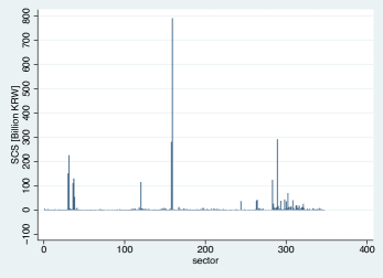
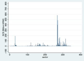
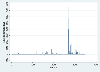
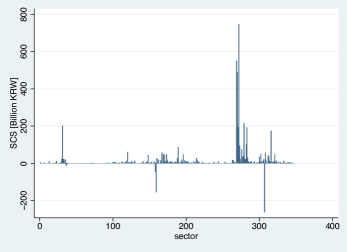
Let us now look into the sectoral distribution of the SCS. Figures 5, 6, 7, and 8 show the projected sector-wise SCS from productivity doubling in the RMC sector under the Leontief, Cobb–Douglas, CES, and CES (all estimates) systems, respectively, for Japan. Corresponding figures for Korea are Figures 9, 10, 11, and 12. As we have anticipated in regard to the previous Proposition, SCS for the Leontief and Cobb–Douglas systems is distributed on the positive side overall. At base, when there is productivity doubling in one sector, its price will be cut in half. The inter-sectoral propagation of that price change will nevertheless be different, depending on the elasticity of factor substitution among the interacting sectors. As for the Leontief system, because factor substitution will not exist in any other sector, the price change of RMC to half its former level will have no effect upon its intermediate demand. Thus, in that event, all the factor inputs (including the primary factor) for the RMC sector will be reduced by half. This is the main reason why the primary factor for the RMC sector is reduced (as SCS) rather prominently for the Leontief system. Consequently, the intermediate demand of the factors (including the primary factor) will be reduced respectively by as much as half the amount that used to go into the RMC sector. Such reduction of intermediate demand and thus of supply will be accumulated in convergence. In other words, at least half of the primary factor put into the RMC sector will be directly reduced, and beyond that, the primary factor in any other sector will be reduced indirectly. Figures 5 and 9 reflect such propagation of productivity doubling in the RMC sector upon primary factor demand under a system of zero elasticity of substitution.

In contrast, as for the Cobb–Douglas system, the intermediate demand for RMC, when its price is reduced to half, must be doubled; that is the very definition of unit elasticity of substitution. Thus, in that event, the monetary output and the factor inputs (including the primary factor) of the RMC sector will not change. As for an elastic CES system with elasticity of substitution larger than unity, the factor demand for RMC becomes larger than two fold, when the price of RMC is reduced by half. And in that event, the factor inputs of the RMC sector can be increased. In either system, since the system of unit cost functions is strictly concave, the price of all factors except that of the primary factor that will stay constant, will converge in a strictly descending manner. Hence, in equilibrium, the primary factor will be mitigated for the sectors where the primary factor becomes relatively expensive compared with other factor inputs. Notably, Figures 6 and 7 indicate that primary factor is reduced (as SCS) rather prominently at sectors, namely, “Public construction of roads” (279th), “Public construction of rivers, drainages and others” (280th), and “Residential construction (non-wooden)” (275th), for Japan. Figures 10 and 11 indicate that “Residential building construction” (289th), “Road construction” (272nd), and “Non-residential building construction” (270th) are prominent for Korea. These sectors are obviously the ones that utilize RMC extensively for production. In other words, the primary factor in these sectors will be substituted by RMC with reduced price.

Figure 5: Sectoral distribution of SCS for productivity doubling of RMC sector (150th) for Leontief system. (Japan)

Figure 6: Sectoral distribution of SCS for productivity doubling of RMC sector (150th) for Cobb–Douglas system. (Japan)

Figure 7: Sectoral distribution of SCS for productivity doubling of RMC sector (150th) for multifactor CES system. (Japan)

Figure 8: Sectoral distribution of SCS for productivity doubling of RMC sector (150th) for multifactor CES (all estimates) system. (Japan)

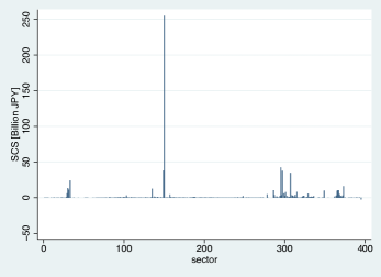
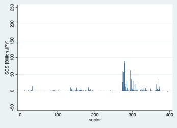
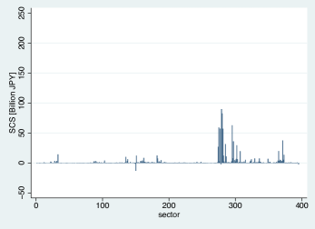
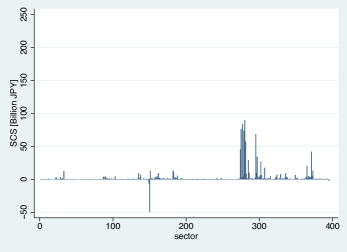
Moreover, we observe from these figures that not only the magnitude of propagation (in terms of SCS) of the productivity stimuli will be magnified by larger elasticities of substitution, but the distribution of SCS become more even. We have measured the “polarity” of the distribution of SCS over the sectors via kurtosis, displayed in parentheses in Table 2. The primary factor will be mitigated primarily at the RMC sector where the productivity is enhanced for the Leontief system, whereas the mitigation of primary factor will spread over the sectors for the Cobb–Douglas and CES. Put differently, the welfare gain of enhanced productivity in one industry is attained mainly as the curtailment of factor inputs of that particular industry while keeping the output level consistent, for the Leontief system, whereas for the Cobb–Douglas and CES systems the reduced price is appreciated by other industries so that their primary factors are reduced by substitution.

Figure 9: Sectoral distribution of SCS for productivity doubling of RMC sector (159th) for Leontief system. (Korea)

Figure 10: Sectoral distribution of SCS for productivity doubling of RMC sector (159th) for Cobb–Douglas system. (Korea)

4 Concluding Remarks

To date input–output analysis has been a one-of-a-kind framework that considers industry-wide propagation when assessing the costs and benefits of new goods and innovations. Input–output analysis, nonetheless, has laid its theory upon the non-substitution theorem, which allows the researcher to study under a fixed technological structure while restricting the subjects of analyses to transformations within the final demand. Substitution of technology will nevertheless take place in any industry when a new technology is actually introduced into any component (industry) of the economy. Larger influence is typically foreseeable for intermediate industries, as they have much larger and wider feedback on economy-wide systems of production.

In order to consider all technology substitution possibilities, we proposed in this study a methodology to measure the sector specific substitution elasticity for the CES production function, rather than using uniform a priori substitution elasticity (such as zeros and ones), when modeling the economy-wide multisector multifactor production system. A dual analytical method (i.e., unit cost functions) was used to evaluate influences upon general equilibrium technological substitutions and eventually upon social costs and benefits, initiated by the introduction of innovation, which we treat as gains in productivity. We have found that the more elastic production functions (Cobb–Douglas and CES) have more significant and wider propagation effects, whereas inelastic production functions (Leontief) have effects that are relatively less and polarized. Applications and extensions of this framework can perhaps be immense, including internationalization, dynamicalization, and quality considerations all remaining for future investigations.

Figure 11: Sectoral distribution of SCS for productivity doubling of RMC sector (159th) for CES system. (Korea)

Figure 12: Sectoral distribution of SCS for productivity doubling of RMC sector (159th) for multifactor CES (all estimates) system. (Korea)

Appendix

CES Elasticities and Productivity Growths (Japan 2000–2005) sector Elasticity TFPg Obs.
Table Continued
sector Elasticity TFPg Obs.
l.l.l. Liquid crystal element & 2.296 *** 1.269 *** (***) 116
Turbines 1.689 *** 0.783 *** (***) 119
Video recording and playback equipment 2.007 *** 0.773 *** (***) 136
Personal Computers 1.455 * 0.647 126
Coal products 1.979 ** 0.593 (***) 91
Frozen fish and shellfish 2.074 * 0.449 (***) 80
Electronic computing equipment (accessory equipment) 1.871 *** 0.412 ** (***) 132
Cyclic intermediates 1.784 *** 0.367 (***) 105
Fowls and broilers 2.199 * 0.332 (***) 57
Steel ships 1.451 *** 0.307 ** (***) 157
Photographic sensitive materials 1.581 ** 0.283 (**) 106
Other business services 2.098 *** 0.270 (***) 122
Electronic computing equipment (except personal computers) 1.668 *** 0.268 126
Financial service 0.275 * 0.260 (***) 101
Social welfare (profit-making) 1.268 *** 0.251 (***) 143
Private non-profit institutions serving households, n.e.c. * 1.391 * 0.242 (***) 105
Repair of ships 1.378 ** 0.239 (***) 142
Inorganic pigment 1.581 ** 0.233 (***) 104
Other iron or steel products 1.345 * 0.231 81
Public administration (central) ** 1.603 *** 0.223 (***) 219
Boilers 1.646 ** 0.217 (***) 120
Aliphatic intermediates 1.461 * 0.214 (**) 109
Household electric appliances (except air-conditioners) 1.333 ** 0.182 153
Medical service (medical corporations, etc.) 1.622 ** 0.168 (**) 156
Synthetic dyes 1.868 *** 0.165 (***) 97
Dishes, sushi and lunch boxes 1.761 ** 0.165 (***) 116
Applied electronic equipment 1.455 ** 0.160 (*) 133
Railway transport (freight) 1.918 *** 0.154 (***) 101
Noodles 1.669 ** 0.151 (*) 108
Motor vehicle parts and accessories 1.701 *** 0.137 * (**) 152
Dextrose, syrup and isomerized sugar 1.405 ** 0.133 (**) 78
Medicaments 1.976 * 0.132 135
Electric bulbs 1.570 ** 0.125 (*) 103
Other electrical devices and parts 2.059 *** 0.121 125
Other general industrial machinery and equipment 1.386 * 0.116 140
Other industrial organic chemicals 1.687 * 0.115 118
Metal containers, fabricated plate and sheet metal 1.780 *** 0.104 ** (**) 134
Metallic furniture and fixture 1.775 ** 0.103 124
Nursing care (In-facility) 1.585 *** 0.101 (**) 159
Semiconductor making equipment 1.453 ** 0.099 142
Marine culture 1.717 ** 0.092 92
Other metal products 1.774 *** 0.087 (*) 145
Bearings 1.627 *** 0.086 114
Pumps and compressors 2.111 *** 0.085 (**) 129
Wheat, barley and the like 2.952 * 0.081 60
Confectionery 1.807 *** 0.080 121
Other educational and training institutions (profit-making) 1.748 ** 0.079 74
Sporting and athletic goods 1.578 ** 0.077 135
Cosmetics, toilet preparations and dentifrices 1.576 * 0.074 105
Tires and inner tubes 1.517 * 0.072 102
Miscellaneous manufacturing products 1.622 *** 0.071 180
Gas and oil appliances and heating and cooking apparatus 1.568 *** 0.069 133
Agricultural public construction 2.039 * 0.062 144
Health and hygiene (profit-making) 1.509 ** 0.059 94
Plumber’s supplies, powder metallurgy products and tools 1.596 *** 0.057 128
Internal combustion engines for vessels 1.808 ** 0.057 115
Other rubber products 1.740 *** 0.052 125
Electric wires and cables 1.566 *** 0.051 121
Other final chemical products 1.782 *** 0.048 150
Activities not elsewhere classified 3.575 *** 0.047 179
Paint and varnishes 1.703 *** 0.047 125
Oil and fat industrial chemicals 1.555 * 0.047 91
Compressed gas and liquefied gas 1.593 * 0.041 81
Metal products for construction 1.497 ** 0.040 136
Other pulp, paper and processed paper products 1.517 ** 0.035 125
Metal molds 1.894 *** 0.035 127
Health and hygiene (public) ** 1.496 *** 0.033 91
Machinery for agricultural use 1.576 ** 0.030 142
Publication 1.470 * 0.029 105
Other special machinery for industrial use 1.646 ** 0.026 146
Other industrial inorganic chemicals 1.643 ** 0.026 116
Abrasive 1.363 * 0.025 126
Other services relating to communication 2.444 *** 0.019 65
Advertising services 1.964 *** 0.018 103
Electron tubes 1.825 *** 0.018 116
Retort foods 1.543 * 0.012 92
Chemical fertilizer 1.608 * 0.012 113
Internal combustion engines for motor vehicles and parts 1.803 *** 0.010 131
Other structural clay products 1.485 ** 0.010 107
Newspaper 1.529 ** 0.007 99
Wooden furniture and fixtures 2.086 *** 0.004 145
Coated steel 1.981 *** 0.004 100
Miscellaneous ceramic, stone and clay products 1.455 *** 0.004 147
Cement 1.577 ** 0.000 103
Glass fiber and glass fiber products, n.e.c. 1.774 *** -0.002 106
Conveyors 1.408 ** -0.005 138
Fisheries 1.648 *** -0.011 92
Other general machines and parts 1.644 *** -0.013 143
Sewage disposal ** 1.734 *** -0.013 86
Other photographic and optical instruments 0.423 ** -0.014 127
Bread 1.664 ** -0.015 111
Office supplies 2.608 *** -0.015 29
Wiring devices and supplies 1.784 *** -0.019 128
Electrical equipment for internal combustion engines 1.483 ** -0.021 130
Medical service (non-profit foundations, etc.) 1.812 *** -0.021 154
Clay refractories 1.656 *** -0.022 109
Cast and forged materials (iron) 2.091 *** -0.026 133
Engines 1.859 *** -0.026 129
Pulp 2.634 ** -0.028 104
Non-ferrous metal castings and forgings 1.615 ** -0.034 123
Other wooden products 1.716 *** -0.035 160
Railway transport (passengers) 2.086 *** -0.040 112
Sugar 1.492 ** -0.044 83
News syndicates and private detective agencies 1.434 * -0.045 74
Other electronic components 1.746 *** -0.049 152
Electricity 1.476 * -0.052 98
Medical instruments 0.090 *** -0.052 151
Repair of motor vehicles 1.442 * -0.052 114
Repair of rolling stock 1.712 *** -0.052 117
Other glass products 2.006 *** -0.060 107
Bolts, nuts, rivets and springs 1.763 *** -0.060 132
Rolled and drawn aluminum 1.824 * -0.063 86
Synthetic fibers 1.636 * -0.065 99
Woven fabric apparel 1.577 * -0.065 101
Whiskey and brandy 2.601 * -0.071 88
Social welfare (private, non-profit) * 1.460 *** -0.072 143
Knitted apparel 2.031 * -0.084 107
Accommodations 1.825 *** -0.084 (**) 161
Medical service (public) 1.808 *** -0.087 (**) 153
Other transport equipment 1.973 *** -0.089 140
Pottery, china and earthenware 2.073 *** -0.089 (*) 119
Fiber yarns 1.851 ** -0.094 94
Plastic footwear 1.965 *** -0.095 ** (**) 108
Nursing care (In-home) 1.552 *** -0.095 (**) 153
Transformers and reactors 1.600 ** -0.102 124
Cast iron pipes and tubes 1.805 ** -0.102 90
Cleaning 1.655 ** -0.103 (*) 88
Aircrafts 1.684 ** -0.103 121
Food processing machinery and equipment 1.562 ** -0.116 (*) 124
Industrial robots 1.520 ** -0.117 124
Beauty shops 1.459 * -0.126 91
Plywood 1.713 ** -0.126 * 86
Passenger motor cars 1.703 ** -0.135 (*) 123
Audio and video records, other information recording media 1.488 * -0.135 (*) 95
Motor vehicle bodies 1.592 * -0.139 125
Barber shops 1.657 *** -0.148 (***) 86
Repair of machine 1.622 ** -0.153 (*) 145
Plasticizers 2.262 *** -0.153 * (***) 84
Other personal services 1.925 * -0.155 (**) 113
Rolled and drawn copper and copper alloys 1.829 ** -0.166 83
Textile machinery 2.218 *** -0.169 * (***) 138
Rotating electrical equipment 1.457 ** -0.172 (**) 127
Chemical machinery 1.528 ** -0.176 (**) 132
Public baths 1.544 * -0.188 (**) 94
Metal processing machinery 1.654 *** -0.192 ** (***) 128
Petrochemical basic products 1.798 * -0.200 89
Image information production and distribution industry 1.678 ** -0.201 (**) 119
Social welfare (public) ** 1.479 ** -0.201 (***) 142
Hot rolled steel 2.138 *** -0.207 97
Crops for feed and forage 2.988 *** -0.207 *** (***) 58
Crude steel (electric furnaces) 1.870 ** -0.226 96
Machinery for service industry 1.378 ** -0.233 (**) 129
Social education (public) ** 1.812 * -0.238 (***) 93
Consigned freight forwarding -0.732 ** -0.239 (*) 93
Wired communication equipment 2.164 *** -0.243 * (***) 150
Other electrical devices and parts 1.388 ** -0.246 (***) 142
Iron and steel shearing and slitting 2.379 *** -0.265 (*) 83
Other wearing apparel and clothing accessories 1.800 * -0.270 (***) 109
Coal mining , crude petroleum and natural gas 1.850 *** -0.277 *** (***) 89
Rolling stock 1.808 *** -0.284 *** (***) 138
Research and development (intra-enterprise) 1.461 ** -0.317 * (***) 126
Batteries 1.640 ** -0.317 (***) 129
Watches and clocks 1.471 *** -0.339 (***) 121
Wooden chips 1.626 * -0.350 (***) 64
Optical fiber cables 1.634 ** -0.360 (***) 115
Crude steel (converters) 2.635 *** -0.377 ** (***) 99
Electric measuring instruments 1.362 * -0.399 (***) 128
Storage facility service 1.602 ** -0.404 (***) 105
Copper 2.110 ** -0.448 77
Private non-profit institutions serving enterprises 1.586 * -0.450 (***) 91
Other non-ferrous metal products 2.152 ** -0.549 *** (**) 88
Pig iron 1.600 ** -0.680 * (*) 169
Research institutes for natural science (pubic) ** 2.090 * -0.745 * (***) 90
Metallic ores 1.634 *** -0.799 *** (***) 82
Ferro alloys 1.652 * -0.823 85
Research institutes for natural sciences (profit-making) 2.108 ** -0.855 (***) 93


Note: The statistical significances in parenthesis are of the intercept of the regression (2).

CES Elasticities and Productivity Growths (Korea 2000–2005) sector Elasticity TFPg Obs.
Table Continued
sector Elasticity TFPg Obs.
l.l.l. Photographic and optical instruments 2.116 *** 0.688 *** (***) 165
Computer and peripheral equipment 1.660 ** 0.619 (*) 166
Watches and clocks 1.615 ** 0.618 (***) 147
Electric resistors and storage batteries 2.033 *** 0.582 *** (***) 156
Research institutes(private, non-profit, commercial) 1.498 * 0.566 (***) 152
Electric household audio equipment 2.141 *** 0.564 * (***) 151
Misc. amusement and recreation services 1.817 *** 0.514 *** (***) 153
Supporting land transport activities 1.555 ** 0.507 (***) 126
Wood furniture 1.495 * 0.447 (***) 165
Education (commercial) 1.682 ** 0.417 (***) 127
Other audio and visual equipment 1.614 * 0.402 (*) 164
Bicycles and parts and misc. transportation equipment 1.860 *** 0.400 *** (***) 132
Household laundry equipment 1.480 ** 0.399 (***) 145
Electron tubes 1.709 *** 0.393 *** (**) 159
Semiconductor devices 1.542 ** 0.371 162
Road freight transport 1.961 ** 0.370 (***) 131
Printed circuit boards 1.550 ** 0.357 * (*) 160
Section steel 1.520 ** 0.340 (*) 121
Supporting air transport activities 2.164 *** 0.339 ** (***) 108
Business and professional organizations 2.735 *** 0.335 (***) 95
Passenger automobiles 1.674 *** 0.334 ** (***) 155
Office machines and devices 1.536 * 0.332 (**) 154
Industrial glass products 2.121 *** 0.292 *** (**) 169
Central bank and banking institutions, Non-bank depository institutions 1.864 ** 0.287 (***) 120
Water supply 1.675 ** 0.285 (**) 124
Road passenger transport 1.983 *** 0.285 (**) 131
Clay products for construction 1.800 ** 0.285 (**) 140
Lime, gypsum, and plaster products 1.813 * 0.282 (***) 134
Food processing machinery 1.592 ** 0.278 ** (***) 143
Boiler, Heating apparatus and cooking appliances 1.610 * 0.274 (**) 164
Pulp 1.526 * 0.273 112
Medical instruments and supplies 1.793 *** 0.271 (**) 167
Regulators and Measuring and analytical instruments 1.603 ** 0.266 (**) 167
Coastal and inland water transport 1.552 ** 0.265 (***) 134
Leather 1.831 ** 0.260 * (**) 129
Cosmetics and dentifrices 1.974 ** 0.255 * (**) 165
Non-life insurance 1.586 * 0.250 (*) 107
Misc. chemical products 1.589 ** 0.245 (**) 172
Sports organizations and sports facility operation 1.635 *** 0.241 (**) 144
Social work activities(other) 1.757 ** 0.229 (**) 137
Trucks and Motor vehicles with special equipment 1.845 *** 0.229 *** (***) 154
Other membership organizations 1.855 ** 0.225 (**) 114
Wooden containers and Other wooden products 2.034 ** 0.224 (**) 124
Bakery and confectionery products 1.819 * 0.213 (**) 174
Household refrigerators 1.795 *** 0.213 ** (***) 152
Asbestos and mineral wool products 1.754 ** 0.212 (**) 145
Air-conditioning equipment and industrial refrigeration equipment 1.524 ** 0.209 163
Buses and vans 1.736 *** 0.208 (***) 152
Medicaments 1.998 *** 0.207 *** (**) 175
Textile machinery 1.468 * 0.199 165
Silk and hempen fabrics 1.982 ** 0.196 * 110
Printing ink 2.049 *** 0.190 ** (***) 127
Motors and generators 1.731 *** 0.187 ** (**) 161
Misc. non-metallic minerals 2.262 *** 0.185 108
Sanitary services(public) 1.701 ** 0.185 130
Concrete blocks, bricks, and other concrete products 1.891 *** 0.182 ** (***) 144
Lubricants 1.736 * 0.180 131
Pottery 1.560 * 0.177 155
Railroad vehicles and parts 1.537 ** 0.174 157
Metal molds and industrial patterns 1.662 ** 0.169 152
Luggage and handbags 2.172 *** 0.161 ** (***) 118
Pens, pencils, and other artists’ materials 1.794 *** 0.160 ** (*) 145
Motion picture, Theatrical producers, bands, and entertainers 1.619 *** 0.158 (*) 151
Dairy products 1.971 ** 0.157 (*) 144
Publishing 1.473 * 0.154 124
Ship repairing and ship parts 1.799 *** 0.154 ** (**) 151
Misc. nonmetallic minerals products 1.680 * 0.152 140
Household glass products and others 1.940 *** 0.143 ** (*) 136
Agricultural implements and machinery 1.620 *** 0.129 155
Social work activities(public) 2.169 *** 0.124 121
Reproduction of recorded media 1.987 *** 0.123 * (**) 136
Anthracite 2.325 *** 0.122 132
Paints, varnishes, and allied products 1.700 ** 0.118 155
Line telecommunication apparatuses 1.636 ** 0.118 161
Leather wearing apparels 1.845 * 0.116 108
Library, museum and similar recreation related services(public) 1.843 *** 0.112 133
Paper containers 1.927 *** 0.107 132
Knitted clothing accessories 2.204 ** 0.100 116
Synthetic fiber fabrics 1.852 ** 0.097 128
Motorcycles and parts 1.687 ** 0.095 148
Accommodation 1.657 ** 0.094 132
Ginseng products 1.686 * 0.089 104
Sheet glass and primary glass products 1.985 *** 0.088 129
Electric transformers 1.851 *** 0.087 150
Salted, dried and smoked seafoods 3.290 * 0.084 98
Misc. electric equipment and supplies 1.503 * 0.082 155
Printing 1.579 *** 0.081 143
Abrasives 1.710 ** 0.074 142
Cement 2.086 *** 0.070 154
Prepared livestock feeds 1.713 * 0.069 154
Library, museum and similar recreation related services(other) 1.578 * 0.066 135
Knitted fabrics 1.928 ** 0.064 111
Internal combustion engines and turbines 1.649 *** 0.063 156
Fiber bleaching and dyeing 1.949 ** 0.058 119
Cleaning and disinfection services 1.552 * 0.058 104
Other paper products 1.597 * 0.054 160
Other raw paper and paperboard 1.808 *** 0.043 150
Petrochemical intermediate products and Other basic organic chemicals 1.876 ** 0.042 163
Fastening metal products 1.661 ** 0.038 137
Household articles of plastic material 1.721 ** 0.032 124
Stationery paper and office paper 1.497 * 0.032 125
Recording media and Photographic chemical products 1.853 *** 0.031 142
Medical and health services (commercial) 2.288 *** 0.030 160
Ready mixed concrete 2.040 *** 0.030 132
Supporting water transport activities 1.637 ** 0.029 125
Other leather products 1.858 * 0.028 91
Construction and mining machinery 1.577 ** 0.025 156
Nitrogen compounds 1.759 ** 0.025 114
Road construction 1.389 * 0.023 179
Metal products for construction 1.828 ** 0.019 134
Industrial plastic products 1.674 ** 0.014 167
Land clearing and reclamation, and irrigation project construction 1.539 ** 0.009 167
Soy sauce ad bean paste 1.750 * 0.008 127
Communications line construction 1.585 ** 0.006 159
Metal furniture 1.565 ** 0.006 146
Thread and other fiber yarns 1.915 *** -0.004 114
Life insurance 1.627 * -0.005 106
Capacitors and rectifiers, Electric transmission and distribution equipment 1.583 *** -0.005 167
Musical instruments 1.506 ** -0.005 155
Iron foundries and foundry iron pipe and tubes 1.840 *** -0.006 152
Misc. petroleum refinery products 1.793 * -0.011 127
Medical and health services(public) 2.180 *** -0.011 138
Pumps and compressors 1.601 ** -0.018 158
Adhesives, gelatin and sealants 1.882 ** -0.021 143
Rubber products 1.763 *** -0.022 154
Canned or cured fruits and vegetables 1.761 * -0.034 139
Corrugated paper and solid fiber boxes 1.662 ** -0.040 119
Crushed and broken stone abd Other bulk stones 1.787 * -0.044 120
Railroad construction 1.432 * -0.045 170
Medical and health services(Private, non-profit) 1.946 *** -0.046 141
Architectural engineering services 1.606 ** -0.048 143
Newspapers 1.873 *** -0.049 118
Sporting and athletic goods 1.720 * -0.058 159
Treatment and coating of metals and Misc. fabricated metal products 1.722 ** -0.060 171
Synthetic fiber yarn 1.903 ** -0.067 124
Plywood 1.769 * -0.067 122
Electric lamps and electric lighting fixtures 1.575 ** -0.068 160
Synthetic fibers 1.701 * -0.073 128
Research institutes(public) 1.611 ** -0.080 182
Services related to real estate 2.091 ** -0.080 91
Lumber 2.081 ** -0.080 105
Insulated wires and cables 1.777 *** -0.089 169
Other nonferrous metal ingots 1.697 * -0.097 121
Personal services 1.977 *** -0.110 (*) 124
Conveyors and conveying equipment 1.649 ** -0.110 165
Electric power plant construction 1.334 * -0.125 171
Starches 2.220 ** -0.137 (*) 102
Footwear 1.836 *** -0.139 * (*) 131
Other edible crops 2.586 ** -0.139 58
Explosives and fireworks products 1.637 ** -0.156 139
Wooden products for construction 1.953 *** -0.164 ** (**) 114
Bolts, nuts, screws, rivets, and washers 1.688 ** -0.168 * 139
Pig iron 1.922 *** -0.171 138
Railroad passenger transport 2.544 *** -0.181 ** (*) 135
Gold and silver ingots 2.860 *** -0.186 (*) 112
Sand and gravel 2.520 ** -0.201 113
Steel ships 1.549 ** -0.203 181
Telecommunications 1.623 * -0.213 123
Other personal repair services 1.925 *** -0.225 *** (***) 147
Education (public) 1.936 *** -0.231 *** (**) 169
Gasoline and Jet oil 1.698 ** -0.234 127
Other ships 1.888 *** -0.287 *** (***) 166
Forgings 2.125 *** -0.289 *** (**) 122
Cargo handling 1.861 ** -0.373 (***) 122
Research and experiment in enterprise 1.415 ** -0.502 (***) 225
Education (private, non-profit) 1.525 * -0.509 (***) 148


Note: The statistical significances in parenthesis are of the intercept of the regression (2).

References

- Álvarez-Martínez and Polo [2012] Álvarez-Martínez, M.T., Polo, C., 2012. A general equilibrium assessment of external and domestic shocks in spain. Economic Modelling 29, 2486 – 2493. doi:10.1016/j.econmod.2012.06.035.
- Antimiani et al. [2015] Antimiani, A., Costantini, V., Paglialunga, E., 2015. The sensitivity of climate-economy ¥CGE¥ models to energy-related elasticity parameters: Implications for climate policy design. Economic Modelling 51, 38 – 52. doi:10.1016/j.econmod.2015.07.015.
- Arrow et al. [1961] Arrow, K.J., Chenery, H.B., Minhas, B.S., Solow, R.M., 1961. Capital-labor substitution and economic efficiency. Review of Economics and Statistics 43, 225–250.
- Böhringer et al. [2015] Böhringer, C., Rutherford, T.F., Springmann, M., 2015. Clean-development investments: An incentive-compatible CGE modelling framework. Environmental and Resource Economics 60, 633–651. doi:10.1007/s10640-014-9762-3.
- BOK [2015] BOK, 2015. Bank of Korea Economic Statistics System; 1995, 2000, 2005 Linked Input-Output Tables [in Korean]. URL: http://ecos.bok.or.kr.
- Chenery and Watanabe [1958] Chenery, H.B., Watanabe, T., 1958. International comparisons of the structure of production. Econometrica 26, 487–521.
- Diewert [1976] Diewert, W.E., 1976. Exact and superlative index numbers. Journal of Econometrics 4, 115–145.
- Go et al. [2016] Go, D.S., Lofgren, H., Ramos, F.M., Robinson, S., 2016. Estimating parameters and structural change in CGE models using a bayesian cross-entropy estimation approach. Economic Modelling 52, Part B, 790 – 811. doi:10.1016/j.econmod.2015.10.017.
- GTAP [2016] GTAP, 2016. Global Trade Analysis Project. URL: https://www.gtap.agecon.purdue.edu.
- JIP [2015] JIP, 2015. Japan Industrial Productivity Database. URL: http://www.rieti.go.jp/en/database/jip.html.
- KIP [2015] KIP, 2015. Korea Industrial Productivity Database. URL: https://www.kpc.or.kr/eng/Productivity/kip.asp.
- Klein [1952–1953] Klein, L.R., 1952–1953. On the interpretation of professor Leontief’s system. Review of Economic Studies 20, 131–136.
- Koesler and Schymura [2015] Koesler, S., Schymura, M., 2015. Substitution elasticities in a constant elasticity of substitution framework – empirical estimates using nonlinear least squares. Economic Systems Research 27, 101–121. doi:10.1080/09535314.2014.926266.
- Kondo [2014] Kondo, Y., 2014. Triangulation of input–output tables based on mixed integer programs for inter-temporal and inter-regional comparison of production structures. Journal of Economic Structures 3, 1–19. doi:10.1186/2193-2409-3-2.
- Kuroda et al. [1984] Kuroda, M., Yoshioka, K., Jorgenson, D.W., 1984. Relative price changes and biases of technical change in Japan. Economic Studies Quarterly 35, 116–138.
- Lin [2000] Lin, L.I.K., 2000. A note on the concordance correlation coefficient. Biometrics 56, 324–325. doi:10.1111/j.0006-341X.2000.00324.x.
- McFadden [1963] McFadden, D., 1963. Constant elasticity of substitution production functions. Review of Economic Studies 30, 73–83.
- McKibbin and Wilcoxen [1999] McKibbin, W.J., Wilcoxen, P.J., 1999. The theoretical and empirical structure of the g-cubed model. Economic Modelling 16, 123 – 148. doi:10.1016/S0264-9993(98)00035-2.
- MIAC [2011] MIAC, 2011. Ministry of Internal Affaris and Communications 1995–2000–2005 Linked Input-Output Tables [in Japanese]. URL: http://www.soumu.go.jp/main_content/000291877.pdf.
- Saito and Tokutsu [1989] Saito, M., Tokutsu, I., 1989. An international comparison of the multi-sectoral production structure – U.S.A., West Germany and Japan, in: Hickman, B. (Ed.), International Productivity and Competitiveness. Oxford University Press.
- Sato [1967] Sato, K., 1967. A two level constant elasticity of substitution production function. Review of Economic Studies 34, 116–138.
- Star and Hall [1976] Star, S., Hall, R.E., 1976. An approximate Divisia index of total factor productivity. Econometrica 44, 257–263.
- Tokutsu [1994] Tokutsu, I., 1994. Price-endogenized input–output model: A general equilibrium analysis of the production sector of the Japanese economy. Economic Systems Research 6, 323–346. doi:10.1080/09535319400000028.
- Uzawa [1962] Uzawa, H., 1962. Production functions with constant elasticities of substitution. Review of Economic Studies 29, 291–299.
- Welsch [2006] Welsch, H., 2006. Armington elasticities and induced intra-industry specialization: The case of France, 1970-1997. Economic Modelling 23, 556 – 567. doi:10.1016/j.econmod.2006.02.008.
- van der Werf [2008] van der Werf, E., 2008. Production functions for climate policy modeling: An empirical analysis. Energy Economics 30, 2964 – 2979. doi:10.1016/j.eneco.2008.05.008.