A Belief Propagation Based Framework for Soft Multiple-Symbol Differential Detection

Abstract

Soft noncoherent detection, which relies on calculating the a posteriori probabilities (APPs) of the bits transmitted with no channel estimation, is imperative for achieving excellent detection performance in high-dimensional wireless communications. In this paper, a high-performance belief propagation (BP)-based soft multiple-symbol differential detection (MSDD) framework, dubbed BP-MSDD, is proposed with its illustrative application in differential space-time block-code (DSTBC)-aided ultra-wideband impulse radio (UWB-IR) systems. Firstly, we revisit the signal sampling with the aid of a trellis structure and decompose the trellis into multiple subtrellises. Furthermore, we derive an APP calculation algorithm, in which the forward-and-backward message passing mechanism of BP operates on the subtrellises. The proposed BP-MSDD is capable of significantly outperforming the conventional hard-decision MSDDs. However, the computational complexity of the BP-MSDD increases exponentially with the number of MSDD trellis states. To circumvent this excessive complexity for practical implementations, we reformulate the BP-MSDD, and additionally propose a Viterbi algorithm (VA)-based hard-decision MSDD (VA-HMSDD) and a VA-based soft-decision MSDD (VA-SMSDD). Moreover, both the proposed BP-MSDD and VA-SMSDD can be exploited in conjunction with soft channel decoding to obtain powerful iterative detection and decoding based receivers. Simulation results demonstrate the effectiveness of the proposed algorithms in DSTBC-aided UWB-IR systems.

I Introduction

Coherent detection has been widely investigated and successfully applied in many wireless communication systems [1]. However, coherent detection requires accurate channel state information, which becomes expensive or even infeasible to obtain in certain scenarios, such as ultra-wideband impulse radio (UWB-IR) systems, massive multiple-input multiple-output (MIMO) systems, millimeter communications, dense wireless networks and so on [1]-[3]. Therefore, noncoherent detection avoiding channel estimation has attracted growing research interests [2], [4]. Noncoherent detection techniques primarily rely on differential detection (DD) [4, 5]. Due to the doubled variance of the effective noise, the standard one-symbol DD suffers 3dB signal-to-noise ratio (SNR) loss in the bit-error rate (BER) performance compared to their coherent counterparts. To circumvent this dilemma, multiple-symbol differential detection (MSDD) has been advocated as an effective algorithm for improving the detection performance of differential receivers [6]-[11]. By exploiting an increased observation window size, MSDD is capable of flexibly reducing the BER performance gap between noncoherent and coherent detection.

Noncoherent detection also leads to promising low-complexity and energy-efficient receivers for multipath fading channels [12]. As a milestone for reliable communication over multipath fading channels, multi-antenna based space-time block-codes (STBC) were invented in [13], which substantially improved the BER performance compared to the single-antenna systems. Furthermore, DD-based STBC (DSTBC) systems were proposed in [14]. In order to reduce the SNR loss facing the DD scheme of [14], an MSDD algorithm was conceived for DSTBC systems in [15]. Generalized likelihood ratio test based MSDD (GLRT-MSDD), decision feedback based MSDD and sphere decoding based MSDD (SD-MSDD) were investigated for the DSTBC aided systems in [16, 17]. However, the aforementioned MSDD algorithms are all based on hard-decision detection, whose BER performance often remains unsatisfactory. By comparison, soft-decision based iterative MSDD has been perceived as a more promising algorithm for improving the detection performance in channel-coded systems [18]-[21], where MSDD is typically concatenated in an iterative manner [22] with the decoder of an error-correcting code (ECC) that is capable of generating soft outputs, such as convolutional codes, turbo codes and low-density parity-check codes [22]-[25]. In iterative MSDD schemes of channel-coded systems, how to calculate the a posteriori probability (APP) of each bit transmitted becomes the key problem of interest.

Owing to the appealing benefit of forward-and-backward message passing, belief propagation (BP) has been successfully applied in many applications, especially in iterative receiver design [26]-[32]. However, most of them are investigated in the context of coherent detection systems. To the best of our knowledge, no BP-based soft-input soft-output (SISO) MSDD has been proposed in the open literature in noncoherent DSTBC-aided UWB-IR systems.

Against the above background, in this paper, our aim is to design a BP-based SISO MSDD framework with its illustrative application in the DSTBC aided UWB-IR systems. Our particular attention is focused on how to calculate the APPs of the information bits transmitted. As such, firstly, an equivalent channel model is proposed for MSDD that relies on sampling with an autocorrelation receiver (AcR) architecture. Furthermore, we describe the AcR sampling with a trellis structure and then decompose the trellis into multiple subtrellises. As a beneficial result, the bidirectional message passing of BP is performed on these subtrellises, and a mathematical framework for soft MSDD, dubbed BP-MSDD, is obtained. Since all subtrellises are taken into account, our BP-MSDD is capable of generating reliable a posteriori information. Notably, the proposed BP-MSDD is capable of achieving more competitive detection performance than the existing GLRT-MSDD advocated for the DSTBC aided UWB systems. However, the computational complexity of the BP-MSDD increases exponentially with the number of MSDD trellis states. Additionally, as a common feature of MSDD schemes, BP-MSDD also exhibits high computational complexity when the observation window size increases. To circumvent the excessive complexity of BP-MSDD, we further propose a Viterbi algorithm (VA)-based hard-decision MSDD (VA-HMSDD) and a VA-based soft-decision MSDD (VA-SMSDD), which constitute attractive practical alternatives due to their advantage over BP-MSDD in terms of performance-versus-complexity tradeoff. Additionally, the proposed BP-MSDD and VA-SMSDD can be exploited in conjunction with soft channel decoder to conduct iterative detection and decoding (IDD). Hence, they are particularly attractive for the noncoherent systems. For example, due to the high frequency selectivity and dense multipaths of UWB-IR channels [33], noncoherent UWB-IR systems are preferred because of their low implementation complexity. Although the proposed MSDD algorithms can generally be used in a number of noncoherent detection scenarios, for the sake of convenience, in this paper our numerical simulations are carried out in the context of DSTBC aided UWB-IR systems to validate the effectiveness of the proposed algorithms. For explicit clarity, the main contributions of this paper are summarized as follows.

• An equivalent channel model is developed with the aid of a rigorous theoretic analysis in the context of DSTBC aided UWB-IR systems. This model is attractive, because relying on this model, accurate soft information can be efficiently obtained for MSDD.

• Inspired by the forward-and-backward message passing mechanism of BP, the BP-MSDD is conceived, of which the message passing mechanism is implemented on the DSTBC trellis diagram. In contrast to the existing MSDD algorithms of [16], [17], the proposed BP-MSDD exclusively benefits from its bidirectional passing mechanism.

• In order to circumvent the excessive complexity of BP-MSDD for practical applications, the survivor paths of the GLRT-MSDD trellises are obtained by reducing the number of trellis states, and correspondingly, the VA-HMSDD is proposed, in which the maximum tolerable computational complexity can be restricted through a proper selection of the VA memory depth. This advantage is particularly attractive, because the prohibitive computational complexity of the GLRT-MSDD trellises is one of the major challenges facing the BP-MSDD.

• Upon extending the trellis-based detection further, the VA-SMSDD is designed for enhancing the detection performance of VA-HMSDD. Another benefit of the VA-SMSDD is that it also enjoys a lower computational complexity than the BP-MSDD. More specifically, the computational complexity of BP-MSDD increases exponentially with the number of the trellis states. By contrast, VA-SMSDD has a computational complexity increasing only linearly with the number of trellis states, although its BER performance is slightly degraded compared with that of BP-MSDD.

We emphasize that the MSDD algorithms proposed in this paper can be extended and applied in many other communication systems after necessary minor adaptations. For example, several MSDD schemes have been developed for the symbol detection in differential phase shift keying (DPSK) aided systems as well as differential space-time encoded MIMO systems [19]. In particular, we consider the DSTBC aided UWB-IR system just as an application for illustrating the principle of the proposed MSDDs. The UWB-IR system exploits narrow pulses of nanoseconds to transmit information bits, and the received signal consists of a large number of resolvable multipath components after passing through the UWB-IR channel. Hence, the stringent requirement imposed on channel estimation makes it difficult and costly to implement the optimal coherent receiver. Thus, noncoherent detection becomes inevitable in UWB-IR systems. In what follows, the proposed BP-MSDD, VA-HMSDD and VA-SMSDD will be investigated in the context of DSTBC aided UWB-IR systems.

The rest of this paper is organized as follows. In Section II, we introduce the DSTBC system model. In Section III, we commence with a brief review of the AcR-based MSDD with the aid of an equivalent channel model, then the BP-MSDD is proposed relying on this model, which is followed by formulating both the VA-HMSDD and the VA-SMSDD for reducing the computational complexity. Our simulation results are provided in Section IV. Finally, conclusions are drawn in Section V.

Notations: Lower-case (upper-case) boldface symbols denote vectors (matrices); ${\mathbf{I}}_{H}$ represents the $H\times H$ identity matrix; $(\cdot)^{\mathrm{T}}$ and $\mathrm{Tr}{(\cdot)}$ represent the transpose and the trace of a matrix, respectively; $\|\cdot\|_{\mathrm{F}}$ denotes the Frobenius-norm of a matrix; $\mathrm{E}[\cdot]$ and $\mathrm{Var}[\cdot]$ denote the expectation and the variance of a random variable, respectively; $*$ stands for convolution; $\propto$ means "is proportional to"; $\mathrm{p}(\cdot)$ stands for the probability density function of a continuous random variable; $\mathrm{Pr}(\cdot)$ denotes a probability; both $\sum\limits_{\mathbf{U}:\sim\mathbf{U}_{i}}$ and $\sum\limits_{\sim\mathbf{U}_{i}}$ represent the summation of all the variables in $\mathbf{U}$ except for $\mathbf{U}_{i}$.

II System Description

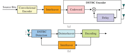
Fig. 1: The diagram of a DSTBC system. (a) and (b) denote a two-antenna transmitter and a $Q$-antenna receiver, respectively.

For illustrative purpose, we consider a DSTBC aided UWB-IR system equipped with two transmit antennas and $Q$ ($Q\geq 1$) receive antennas. The diagram of a basic DSTBC system is demonstrated in Fig. 1. Firstly, the information bits are encoded with an ECC, e.g., a convolutional code. Then, the coded bits are interleaved and fed into the DSTBC encoder. As shown in [34], the channel-encoded information bits are divided into blocks, and then every two bits are mapped onto an information-bearing space-time coded symbol. Each symbol is selected from the code book $\Omega=\{\mathbf{U}^{0},\mathbf{U}^{1},\mathbf{U}^{2},\mathbf{U}^{3}\}$ according to the rule of $00:\mathbf{U}^{0}\rightarrow\left(\begin{array}[]{ccc}1&0\\ 0&1\\ \end{array}\right)$, $01:\mathbf{U}^{1}\rightarrow\left(\begin{array}[]{ccc}-1&0\\ 0&-1\\ \end{array}\right)$, $10:\mathbf{U}^{2}\rightarrow\left(\begin{array}[]{ccc}0&1\\ -1&0\\ \end{array}\right)$, $11:\mathbf{U}^{3}\rightarrow\left(\begin{array}[]{ccc}0&-1\\ 1&0\\ \end{array}\right)$. Each codeword $\mathbf{U}^{f}\in\Omega,f=0,1,2,3$, is constructed according to the property $\mathbf{U}^{f}(\mathbf{U}^{f})^{\mathrm{T}}=(\mathbf{U}^{f})^{\mathrm{T}}\mathbf{U}^{f}=\mathbf{I}_{2}$. Note that each codeword employed in the DSTBC system has to be a unitary matrix. It is well known that for a unitary matrix, each row (column) and the other rows (columns) are mutually orthogonal. When the unitary matrices are designed according to the DSTBC scheme of [13], the proposed algorithms can be extended to systems having more than two transmit antennas. Furthermore, upon invoking the differential encoding, the coded symbol to be transmitted is obtained by

$$\mathbf{D}_{i+1}=\mathbf{D}_{i}\mathbf{U}_{i+1},$$ (1)

where the space-time coded information symbol satisfies $\mathbf{U}_{i+1}\in\Omega$, the $2\times 2$ matrix $\mathbf{D}_{i+1}$ is sent with two antennas during two frame durations, the reference symbol for differential encoding is set to $\mathbf{D}_{0}=\left(\begin{array}[]{cc}1&-1\\ 1&1\\ \end{array}\right)$, $i=0,1,\cdots,N-1$, and $N$ represents the number of differentially encoded symbols to be transmitted. Let $d_{p,2i+n-1}$ denote the entry in the $p$th row and the $n$th column of the matrix $\mathbf{D}_{i}$, where $p=1,2$ and $n=1,2$. Then, the signal transmitted from the $p$th antenna is given by

$$\begin{split}s_{p}(t)&=\sum\limits_{i=0}^{N-1}\sum\limits_{n=1}^{2}d_{p,2i+n-1}\omega(t-(n-1)T_{\mathrm{f}}-iT_{\mathrm{s}})\\ &=\sum\limits_{i=0}^{N-1}\sum\limits_{n=1}^{2}d_{p,2i+n-1}\omega(t-(2i+n-1)T_{\mathrm{f}})\\ &=\sum\limits_{j=0}^{2N-1}d_{p,j}\omega(t-jT_{\mathrm{f}}),\end{split}$$ (2)

where $\omega(t)$ denotes the monocycle pulse that is real-valued waveform with a very short duration $T_{\mathrm{\omega}}$; $t$ is the continuous time index; $T_{\mathrm{f}}$ is the frame duration, which is usually hundreds to thousands times of $T_{\mathrm{\omega}}$ [11]; a single transmitted-symbol duration is $T_{\mathrm{s}}=2T_{\mathrm{f}}$, which implies that in the UWB-IR system considered, two frames are employed to transmit one space-time symbol, and each frame includes one very short pulse; the discrete time index $j=2i+n-1$ is introduced to replace the two-dimensional index $(i,n)$ and $d_{p,2i+n-1}$ is rewritten as $d_{p,j}$, correspondingly. We consider a quasi-static dense multipaths fading environment [33], then the UWB channel impulse response between the $p$th transmit antenna and the $q$th ($1\leq q\leq Q$) receive antenna is formulated as

$$h_{p,q}(t)=\sum\limits_{l=1}^{L_{p,q}}\alpha_{l}^{p,q}\delta(t-\tau_{l}^{p,q}),$$ (3)

where $L_{p,q}$ denotes the number of propagation paths; $\alpha_{l}^{p,q}$ and $\tau_{l}^{p,q}$ are the path-gain coefficient and the delay associated with the $l$th path, respectively; and $\delta(t)$ is Dirac delta function. As a result, the overall channel response between the $p$th transmit antenna and the $q$th receive antenna is expressed as

$$g_{p,q}(t)=\omega(t)*h_{p,q}(t)=\sum\limits_{l=1}^{L_{p,q}}\alpha_{l}^{p,q}\omega(t-\tau_{l}^{p,q}).$$ (4)

Then, the signal at the $q$th receive antenna is given by

$$\begin{split}y_{q}(t)&=\sum\limits_{p=1}^{2}s_{p}(t)*h_{p,q}(t)+n_{q}(t)\\ &=\sum\limits_{p=1}^{2}\sum\limits_{j=0}^{2N-1}d_{p,j}g_{p,q}\left(t-jT_{\mathrm{f}}\right)+n_{q}(t),\end{split}$$ (5)

where $n_{q}(t)$ denotes the additive white Gaussian noise (AWGN) having zero mean and two-sided power spectral density $N_{0}/2$.

III BP-MSDD for DSTBC Aided UWB-IR Systems

Several noncoherent detection schemes have been developed in the context of UWB systems in [16], [17], [34]. Note that most of these MSDD schemes are based on hard-decision, which results in unsatisfactory detection performance in many applications. In general, soft-decision based MSDDs are expected to be capable of outperforming their hard-decision based counterparts. However, soft MSDD remains an inadequately studied topic and few contributions are found in open literature [19]-[21]. A linear prediction algorithm was proposed in [19] to utilize the temporal correlation of fading and a soft information aided iterative multiple-symbol noncoherent detection scheme was conceived for differential unitary space-time modulation in Rayleigh flat fading channels. Furthermore, the authors of [20] developed an iterative detector for coded differential phase shift keying (DPSK) modulated signals in an AWGN channel with unknown phase. Additionally, a simplified iterative SD-MSDD algorithm was developed for DPSK modulated signals in [21], where a Rayleigh-fading channel was considered. These existing soft MSDDs can provide soft information with acceptable quality for detection. However, it is necessary to develop a more sophisticated soft MSDD algorithm, which ought to be capable of achieving much better detection performance. In this section, a soft-decision based BP-MSDD is proposed to tackle this problem in the context of DSTBC aided UWB-IR systems. Firstly, an equivalent channel model is presented for MSDD relying on a novel AcR structure, where the sampling mechanism is judiciously modified and the observation window slides only a single symbol duration $T_{\mathrm{s}}$ each time. This sampling mechanism is different from the $M$-symbol-duration sliding sampling mechanism used in [19]. Then, BP-MSDD is proposed by exploiting this equivalent model and the forward-and-backward message passing mechanism.

III-A Equivalent Channel Model

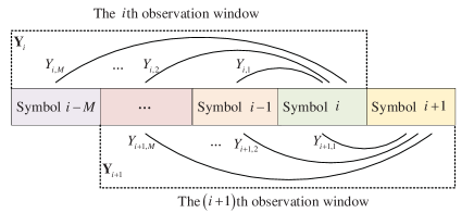
Fig. 2: An illustration of the proposed AcR sampling mechanism for MSDD in the $i$th and $(i+1)$th observation window.

Let us commence with an AcR architecture that is developed for MSDD sampling. For convenience of exposition, the observation window size is set to $M+1$ $(M\geq 1)$ symbol durations, during which the channel is assumed to remain invariant [17], [34]. In [17], the observation window slides forward $M$ symbol durations when the current $M$ symbols have been detected. This is indeed a block-by-block sampling scheme, where the correlations amongst the symbols of different blocks are unfavorably ignored. Motivated by this observation, we obtain a modified symbol-by-symbol sliding mode, in which the observation window slides forward one symbol duration $T_{\mathrm{s}}$ each time. This symbol-by-symbol sampling scheme is particularly suitable for exploiting the correlations among symbols of different blocks, since the detection of each symbol benefits from capitalizing on the information of all the other symbols. In Fig. 2, we illustrate the details of the proposed sampling scheme by examining two adjacent observation windows. To gain more in-depth insights, we formulate the proposed AcR sampling mechanism in a rigorous mathematical manner, and then elaborate on its significance for BP-MSDD. Specifically, in the $i$th observation window represented by $(i-M)T_{\mathrm{s}}\leq t\leq iT_{\mathrm{s}}$, the samples of the received signal are given by $\mathbf{Y}_{i}=[\mathbf{Y}_{i,1},\mathbf{Y}_{i,2},\ldots,\mathbf{Y}_{i,M}]$, where $\mathbf{Y}_{i,m}$ $(m=1,\ldots,M)$ is the correlation function of the received signal and it is formulated as

$$\mathbf{Y}_{i,m}=\sum\limits_{q=1}^{Q}\int_{0}^{T_{\mathrm{i}}}\left(\mathbf{y}_{i}^{q}(t)\right)^{\mathrm{T}}\mathbf{y}_{i-m}^{q}(t)dt,$$ (6)

where $T_{\mathrm{i}}\leq T_{\mathrm{s}}$ is the integration interval, $\mathbf{y}_{i}^{q}(t)=[y_{q}(t+2iT_{\mathrm{f}})\quad y_{q}(t+(2i+1)T_{\mathrm{f}})]$ is the signal waveform vector received at $q$th antenna. The $(u,v)$th entry of $\mathbf{Y}_{i,m}$ can be expressed as $Y_{i,m}(u,v)=\sum\limits_{q=1}^{Q}\int_{0}^{T_{\mathrm{i}}}y_{q}[t+2iT_{\mathrm{f}}+(u-1)T_{\mathrm{f}}]y_{q}[t+2(i-m)T_{\mathrm{f}}+(v-1)T_{\mathrm{f}}]dt$ with $u,v=1,2$. Substituting (5) into $\mathbf{Y}_{i,m}$, we obtain

$$\begin{split}Y_{i,m}(u,v)&=\sum\limits_{q=1}^{Q}\int_{0}^{T_{\mathrm{i}}}\left(\sum\limits_{p=1}^{2}d_{p,2i+u-1}g_{p,q}(t)+n_{i,u}^{q}(t)\right)\\ &\times\left(\sum\limits_{p=1}^{2}d_{p,2(i-m)+v-1}g_{p,q}(t)+n_{(i-m),v}^{q}(t)\right)dt,\end{split}$$ (7)

where $n_{i,u}^{q}(t)=n_{q}[t+(2i+u-1)T_{\mathrm{f}}]$, and $n_{(i-m),v}^{q}(t)=n_{q}[t+(2i-2m+v-1)T_{\mathrm{f}}]$ denote the time-shifted noises.

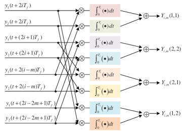
Fig. 3: The illustration of the AcR structure for the $i$th and the $(i-m)$th received symbol matrices of DSTBC aided UWB-IR system having two receive antennas.

The calculation of the correlation matrix (6) requires operations between different segments of the received symbols. Consider $Q=2$ as an example, in Fig. 3 we illustrate the AcR structure for the $i$th and the $(i-m)$th received symbol matrices of DSTBC aided UWB-IR system. For the sake of convenience, we divide ${Y}_{i,m}(u,v)$ into the signal component $S_{i,m}(u,v)$ and the noise component $N_{i,m}(u,v)$. Then, ${Y}_{i,m}(u,v)$ is reformulated as

$$Y_{i,m}(u,v)=S_{i,m}(u,v)+N_{i,m}(u,v),$$ (8)

where $S_{i,m}(u,v)$ is given by

$$\begin{split}&S_{i,m}(u,v)=\\ &\sum\limits_{q=1}^{Q}\int_{0}^{T_{\mathrm{i}}}\Bigg{(}\sum\limits_{p=1}^{2}d_{p,2i+u-1}g_{p,q}(t)\sum\limits_{p=1}^{2}d_{p,2(i-m)+v-1}g_{p,q}(t)\Bigg{)}dt,\end{split}$$ (9)

and $N_{i,m}(u,v)$ can be expressed as

$$N_{i,m}(u,v)=N_{1}+N_{2}+N_{3},$$ (10)

with

$$N_{1}=\sum\limits_{p=1}^{2}d_{p,2i+u-1}\sum\limits_{q=1}^{Q}\int_{0}^{T_{\mathrm{i}}}g_{p,q}(t)n_{(i-m),v}^{q}(t)dt,$$ (11)

$$N_{2}=\sum\limits_{p=1}^{2}d_{p,2(i-m)+v-1}\sum\limits_{q=1}^{Q}\int_{0}^{T_{\mathrm{i}}}g_{p,q}(t)n_{i,u}^{q}(t)dt,$$ (12)

and

$$N_{3}=\sum\limits_{q=1}^{Q}\int_{0}^{T_{\mathrm{i}}}n_{i,u}^{q}(t)n_{(i-m),v}^{q}(t)dt.$$ (13)

Similar to that of [34], we assume that $n_{q}(t)$ is an AWGN process with bandwidth $W\gg 1/T_{\mathrm{i}}$. Clearly, $N_{1}$ and $N_{2}$ are Gaussian random variables, while $N_{3}$ approximately obeys a Gaussian distribution [16]. Given the channel realizations $h=\{h_{p,q}(t)\}$, according to the central limit theorem, $N_{i,m}(u,v)$ in (8) can be considered as a noise which has zero mean and conditional variance

$$\sigma^{2}=\mathrm{Var}[N_{i,m}(u,v)|h]=\mathrm{E}[N_{1}^{2}|h]+\mathrm{E}[N_{2}^{2}|h]+\mathrm{E}[N_{3}^{2}].$$ (14)

For analytical convenience, we define $\varepsilon_{p,q}=\int_{0}^{T_{\mathrm{i}}}h_{pq}^{2}(t)dt$, and $\xi=\sum\limits_{p=1}^{2}\sum\limits_{q=1}^{Q}\varepsilon_{p,q}$. According to (11), (12) and (13), the conditional variance of $N_{1}$, $N_{2}$ and $N_{3}$ can be expressed as $\mathrm{E}[N_{1}^{2}|h]=\mathrm{E}[N_{2}^{2}|h]=\frac{N_{0}}{2}\sum\limits_{p=1}^{2}\sum\limits_{q=1}^{Q}\varepsilon_{p,q}$ and $\mathrm{E}[N_{3}^{2}]=\frac{QWT_{\mathrm{i}}N_{0}^{2}}{2}$, respectively. Substituting $\mathrm{E}[N_{1}^{2}|h]$, $\mathrm{E}[N_{2}^{2}|h]$ and $\mathrm{E}[N_{3}^{2}]$ into (14), we obtain

$$\sigma^{2}=N_{0}\sum\limits_{p=1}^{2}\sum\limits_{q=1}^{Q}\varepsilon_{p,q}+\frac{QWT_{\mathrm{i}}N_{0}^{2}}{2}=N_{0}\xi+\frac{QWT_{\mathrm{i}}N_{0}^{2}}{2}.$$ (15)

Consequently, $\mathbf{Y}_{i,m}$ in (6) can be rewritten as

$$\mathbf{Y}_{i,m}=\mathbf{S}_{i,m}+\mathbf{N}_{i,m},$$ (16)

where $\mathbf{S}_{i,m}=\left(\begin{array}[]{cc}S_{i,m}(1,1)&S_{i,m}(1,2)\\ S_{i,m}(2,1)&S_{i,m}(2,2)\\ \end{array}\right)$ and $\mathbf{N}_{i,m}=\left(\begin{array}[]{cc}N_{i,m}(1,1)&N_{i,m}(1,2)\\ N_{i,m}(2,1)&N_{i,m}(2,2)\\ \end{array}\right)$ represent the signal component and the noise component, respectively. Moreover, based on the differential modulation $\mathbf{D}_{i}=\mathbf{D}_{i-1}\mathbf{U}_{i}$ and $\mathbf{D}_{i}\mathbf{D}_{i}^{\mathrm{T}}=2\mathbf{I}_{2}$, we have

$$\begin{split}&\mathbf{D}_{i}\mathbf{D}_{i-m}^{\mathrm{T}}=\mathbf{D}_{i-1}\mathbf{U}_{i}\mathbf{D}_{i-m}^{\mathrm{T}}\\ &=\mathbf{D}_{i-m}\mathbf{U}_{i-m+1}\cdots\mathbf{U}_{i-1}\mathbf{U}_{i}\mathbf{D}_{i-m}^{\mathrm{T}}=2\prod_{z=i-m+1}^{i}\mathbf{U}_{z}.\end{split}$$ (17)

Jointly considering (16) and (LABEL:differ), we can concisely reformulate $\mathbf{Y}_{i,m}$ as

$$\mathbf{Y}_{i,m}=(\mathbf{D}_{i}\mathbf{D}_{i-m}^{\mathrm{T}})\xi+\mathbf{N}_{i,m}=(2\prod_{z=i-m+1}^{i}\mathbf{U}_{z})\xi+\mathbf{N}_{i,m}.$$ (18)

Therefore, the conditional probability required by the MSDD of DSTBC aided UWB-IR systems in a single observation window is formulated as

$$\begin{split}&\mathrm{p}(\mathbf{Y}_{i}|\mathbf{U}_{i-M+1},\cdots,\mathbf{U}_{i-1},\mathbf{U}_{i})\propto\\ &\prod_{m=1}^{M}\mathrm{exp}\left(-\frac{\|\mathbf{Y}_{i,m}-(2\prod_{z=i-m+1}^{i}\mathbf{U}_{z})\xi\|_{\mathrm{F}}^{2}}{\sigma^{2}}\right),\end{split}$$ (19)

which will be applied into generating reliable a posteriori information for the BP-MSDD with soft-decisions. We assume that $T_{\mathrm{s}}=N_{\mathrm{f}}\cdot T_{\mathrm{f}}$, then in (19) the receivers can employ the energy parameter as $\hat{\xi}=\sqrt{\sum_{i,m}\mathbf{Y}^{2}_{i,m}}/N_{\mathrm{f}}$ [35], where $N_{\mathrm{f}}$ is the number of frames in a single symbol duration $T_{\mathrm{s}}$. After obtaining the sampling result $\mathbf{Y}_{i}$, the next sampling outcome $\mathbf{Y}_{i+1}$ may be calculated based on the next observation window $(i-M+1)T_{\mathrm{s}}\leq t\leq(i+1)T_{\mathrm{s}}$.

Remark 1: The conditional probability (19) can be regarded as a metric function. Relying on the proposed sampling mechanism and metric function of (19), our BP-MSDD is derived in the next subsection. The key insight behind the derivation of the BP-MSDD is that we have to construct a graphical model for the whole sampling packet, where our beliefs in the information symbols propagate throughout the graph with the aid of the BP message passing mechanism.

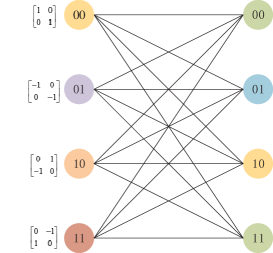
Fig. 4: The DSTBC trellis diagram, where the nodes represented by circles denote the states and the lines represent the branches corresponding to the state transitions. The matrices on the left represent the input information symbols, and the state transition is from the left to the right.

III-B Belief Propagation Based MSDD

Aiming for obtaining the information bits’ maximum APPs, i.e., we use the maximum a posteriori probability (MAP) criterion, our BP-MSDD focuses on the calculations of the bitwise APPs that are denoted by $\Lambda[d_{i}(k)]=\mathrm{p}[d_{i}(k)=z|\mathbf{Y}]$, where $d_{i}(k)$ is the $k$th bit of the information symbol $\mathbf{U}_{i}$, $k=1,2$ and $z=0,1$. Let $\mathbf{Y}\triangleq\{\mathbf{Y}_{i}\}$ be the matrix containing the sampling results of all the observation windows and $\mathbf{U}\triangleq\{\mathbf{U}_{1},\mathbf{U}_{2},\cdots\mathbf{U}_{N}\}$ containing all the information symbols. Then, the APP for $\mathbf{U}_{i}$ is given by

$$\mathrm{Pr}(\mathbf{U}_{i}|\mathbf{Y})=\frac{\mathrm{Pr}(\mathbf{U}_{i},\mathbf{Y})}{\mathrm{p}(\mathbf{Y})}=\frac{\mathrm{p}(\mathbf{Y}|\mathbf{U}_{i})\mathrm{Pr}(\mathbf{U}_{i})}{{\mathrm{p}(\mathbf{Y})}}.$$ (20)

Thus, $\mathbf{U}_{i}$ can be determined with the aid of the MAP criterion as

$$\begin{split}&(\mathbf{U}_{i})_{\mathrm{MAP}}=\mathrm{arg}\max\limits_{\mathbf{U}_{i}}\mathrm{Pr}(\mathbf{U}_{i}|\mathbf{Y})\\ &=\mathrm{arg}\max\limits_{\mathbf{U}_{i}}\frac{\mathrm{p}(\mathbf{Y}|\mathbf{U}_{i})\mathrm{Pr}(\mathbf{U}_{i})}{{\mathrm{p}(\mathbf{Y})}}=\mathrm{arg}\max\limits_{\mathbf{U}_{i}}{\mathrm{p}(\mathbf{Y}|\mathbf{U}_{i})\mathrm{Pr}(\mathbf{U}_{i})},\end{split}$$ (21)

where $\mathrm{p}(\mathbf{Y})$ can be removed, because it is independent of $\mathbf{U}_{i}$. According to (21) and the relationship between the joint probability density function and the marginal probability density function [40], we can obtain

$$\mathrm{Pr}(\mathbf{U}_{i}|\mathbf{Y})\propto\sum_{\mathbf{U}:\sim\mathbf{U}_{i}}\mathrm{p}(\mathbf{Y}|\mathbf{U})\mathrm{Pr}(\mathbf{U}),$$ (22)

which means $\mathrm{Pr}(\mathbf{U}_{i}|\mathbf{Y})\propto\sum_{\mathbf{U}_{1},\mathbf{U}_{2},\cdots,\mathbf{U}_{i-1},\mathbf{U}_{i+1},\cdots,\mathbf{U}_{N}}\mathrm{p}(\mathbf{Y}|\mathbf{U})\mathrm{Pr}(\mathbf{U})$ for any $\mathbf{U}_{i}\in\mathbf{U}$. The direct calculation of (22) imposes a complexity increasing exponentially with $N$. Hence, it is challenging to directly implement it in practical applications when $N$ is large. A reduced-complexity strategy relying on trellis factorization was proposed to address this problem [37]. To elaborate a little further, it was shown in [37] that the global probability function can be factorized into a number of local functions to facilitate the mitigation of inter-symbol interference. Inspired by this innovative idea, we develop a sophisticated framework that is dedicated to noncoherent detection. More specifically, the calculation of (22) can be reformulated as a problem of estimating the APPs of the state transitions of a Markov source [38], which constitutes a discrete finite-state Markov process operating over a noisy discrete memoryless channel (DMC). The indices of the distinct states are indexed by the integer $c$. At the time instant $t^{\prime}$, the source state is denoted by $\mathbf{S}_{t^{\prime}}$ and its output is ${X}_{t^{\prime}}$. A sequence generated by the source is obtained from the state transitions, and the state transition probability of $\mathbf{S}_{t^{\prime}-1}\rightarrow\mathbf{S}_{t^{\prime}}$ is described by $\mathrm{Pr}(c|c^{\prime})=\mathrm{Pr}(\mathbf{S}_{t^{\prime}}=c|\mathbf{S}_{t^{\prime}-1}=c^{\prime})$ and the probability of its output is given by

$$\mathrm{Pr}(X|c^{\prime},c)=\mathrm{Pr}(X=X_{t^{\prime}}|\mathbf{S}_{t^{\prime}-1}=c^{\prime},\mathbf{S}_{t^{\prime}}=c).$$ (23)

In Eq. (24), the values of the states, represented by c’ and c, are certain elements of the state space of the Markov chain. Between each two distinct states, there is a transition probability, which can take any arbitrary value in the interval of [0,1]. For the Markov source, when $X_{1}^{\tau}=[X_{1},X_{2},\cdots,X_{\tau}]$ is the input to a noisy DMC, the output is $Y_{1}^{\tau}=[Y_{1},Y_{2},\cdots,Y_{\tau}]$. For $1\leq t^{\prime}\leq\tau$, the transition probability can be derived as [29]

$$\mathrm{Pr}(Y_{1}^{t^{\prime}}|X_{1}^{t^{\prime}})=\prod_{\eta=1}^{t^{\prime}}\mathrm{Pr}(Y_{\eta}|X_{\eta}).$$ (24)

Based on the above insights, in the following an efficient algorithm is developed to factorize the complicated global function of (22). This factorization is useful for constructing the trellis representation of MSDD, as shown in Fig. 4. In order to obtain the trellis factorization [39] corresponding to MSDD, we define the trellis as follows. Assuming that the state tuple is $\mathbf{S}_{i-1}\triangleq[\mathbf{U}_{i-M},\cdots,\mathbf{U}_{i-1}]^{\mathrm{T}}$, if the input symbol is $\mathbf{U}_{i}$, the output becomes $\mathbf{X}_{i}\triangleq[\mathbf{U}_{i-M+1},\cdots,\mathbf{U}_{i-1},\mathbf{U}_{i}]^{\mathrm{T}}$. The $i$th sampling $\{\mathbf{Y}_{i}\}$ is related to information symbols $\{\mathbf{U}_{i-m}|m=0,\cdots,M-1\}$. In the context of the discrete channel, $\mathrm{p}(\mathbf{Y}|\mathbf{U})$ can be factorized as

$$\mathrm{p}(\mathbf{Y}|\mathbf{U})=\prod_{i=1}^{N}\mathrm{p}(\mathbf{Y}_{i}|\mathbf{U}_{i-M},\cdots,\mathbf{U}_{i-1},\mathbf{U}_{i}),$$ (25)

where $\mathrm{p}(\mathbf{Y}_{i}|\mathbf{U}_{i-M},\cdots,\mathbf{U}_{i-1},\mathbf{U}_{i})$ is given by (19). Correspondingly, $\mathrm{Pr}(\mathbf{U})$ is reformulated as

$$\begin{split}&\mathrm{Pr}(\mathbf{U})=\\ &\prod_{i=1}^{N}\mathrm{Pr}(\mathbf{U}_{i-M},\cdots,\mathbf{U}_{i-1},\mathbf{U}_{i}|\mathbf{U}_{i-M-1},\cdots,\mathbf{U}_{i-2},\mathbf{U}_{i-1}).\end{split}$$ (26)

Furthermore, the local check function for the state transition $\mathbf{S}_{i-1}\rightarrow\mathbf{S}_{i}$ is given by

$$\mathrm{T}_{i}(\mathbf{U}_{i},\mathbf{X}_{i},\mathbf{S}_{i-1},\mathbf{S}_{i})=\left\{\begin{array}[]{ll}1,\quad\mathrm{if}\quad\mathrm{this}\quad\mathrm{event}\quad\mathrm{exists}\\ 0,\quad\mathrm{otherwise},\end{array}\right.$$ (27)

which is also proportional to the state transition probability. Explicitly, we have

$$\begin{split}&\mathrm{T}_{i}(\mathbf{U}_{i},\mathbf{X}_{i},\mathbf{S}_{i-1},\mathbf{S}_{i})\propto\\ &\mathrm{Pr}(\mathbf{U}_{i-M},\cdots,\mathbf{U}_{i-1},\mathbf{U}_{i}|\mathbf{U}_{i-M-1},\cdots,\mathbf{U}_{i-2},\mathbf{U}_{i-1}).\end{split}$$ (28)

Based on (26), (27) and (LABEL:statetrans), $\mathrm{Pr}(\mathbf{U})$ satisfies

$$\mathrm{Pr}(\mathbf{U})\propto\prod_{i=1}^{N}\mathrm{T}_{i}(\mathbf{U}_{i},\mathbf{X}_{i},\mathbf{S}_{i-1},\mathbf{S}_{i}).$$ (29)

Defining $\mathrm{Pr}(\mathbf{U}_{i})$ as the a priori probability of $\mathbf{U}_{i}$ and substituting (25), (29) into (22), we have

$$\begin{split}&\mathrm{Pr}(\mathbf{U}_{i}|\mathbf{Y})\varpropto\\ &\underbrace{\left(\sum\limits_{\mathbf{U}_{1:i-1}}\prod_{w=1}^{i-1}\mathrm{Pr}(\mathbf{U}_{w})\mathrm{p}(\mathbf{Y}_{w}|\mathbf{X}_{w})\mathrm{T}_{w}(\mathbf{U}_{w},\mathbf{X}_{w},\mathbf{S}_{w-1},\mathbf{S}_{w})\right)}_{\triangleq\alpha(\mathbf{S}_{i-1})}\times\\ &\mathrm{Pr}(\mathbf{U}_{i})\mathrm{p}(\mathbf{Y}_{i}|\mathbf{X}_{i})\mathrm{T}_{i}(\mathbf{U}_{i},\mathbf{X}_{i},\mathbf{S}_{i-1},\mathbf{S}_{i})\times\\ &\underbrace{\left(\sum\limits_{\mathbf{U}_{i+1:N}}\prod_{w=i+1}^{N}\mathrm{Pr}(\mathbf{U}_{w})\mathrm{p}(\mathbf{Y}_{w}|\mathbf{X}_{w})\mathrm{T}_{w}(\mathbf{U}_{w},\mathbf{X}_{w},\mathbf{S}_{w-1},\mathbf{S}_{w})\right)}_{\triangleq\beta(\mathbf{S}_{i})},\end{split}$$ (30)

where the first part behind "$\propto$" denotes the forward-probabilities $\alpha(\mathbf{S}_{i})$ and they are given by

$$\begin{split}\alpha(\mathbf{S}_{i})\propto\sum_{\sim\mathbf{S}_{i}}\alpha(\mathbf{S}_{i-1})\mathrm{Pr}(\mathbf{U}_{i})\mathrm{p}(\mathbf{Y}_{i}|\mathbf{X}_{i})\mathrm{T}_{i}(\mathbf{U}_{i},\mathbf{X}_{i},\mathbf{S}_{i-1},\mathbf{S}_{i}).\end{split}$$ (31)

Similarly, in (30) the third part behind "$\propto$" represents the backward-probabilities $\beta(\mathbf{S}_{i})$, which are obtained as

$$\begin{split}&\beta(\mathbf{S}_{i})\propto\sum_{\sim\mathbf{S}_{i+1}}\\ &\beta(\mathbf{S}_{i+1})\mathrm{Pr}(\mathbf{U}_{i+1})\mathrm{p}(\mathbf{Y}_{i+1}|\mathbf{X}_{i+1})\mathrm{T}_{i+1}(\mathbf{U}_{i+1},\mathbf{X}_{i+1},\mathbf{S}_{i},\mathbf{S}_{i+1}).\end{split}$$ (32)

In summary, the a posteriori information in our BP-MSDD can be calculated by using

$$\begin{split}&\mathrm{Pr}(\mathbf{U}_{i}|\mathbf{Y})\propto\sum_{\sim\mathbf{U}_{i}}\\ &\alpha(\mathbf{S}_{i-1})\beta(\mathbf{S}_{i})\mathrm{p}(\mathbf{Y}_{i}|\mathbf{X}_{i})\mathrm{Pr}(\mathbf{U}_{i})\mathrm{T}_{i}(\mathbf{U}_{i},\mathbf{X}_{i},\mathbf{S}_{i-1},\mathbf{S}_{i}).\end{split}$$ (33)

Finally, the channel decoder calculates the decision statistics $\imath(d_{i}(k))\triangleq\mathrm{p}(\mathbf{U}_{i}|\mathbf{Y})_{d_{i}(k)=1}-\mathrm{p}(\mathbf{U}_{i}|\mathbf{Y})_{d_{i}(k)=0}$. If $\imath(d_{i}(k))\geq 0$, we have $\hat{d}_{i}(k)=1$. Otherwise, we have $\hat{d}_{i}(k)=0$.

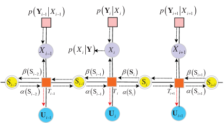
Fig. 5: The factor graph representation of the proposed BP-MSDD, where the larger circles are the variable nodes corresponding to the inputs and the outputs, the smaller circles represent the variable nodes corresponding to the states, while the squares are the factor nodes characterizing the check functions. Additionally, the black arrows denote the directions of the BP message passing, and the red arrows denote the information sent from the detector to the decoder.

In order to thoroughly understand the proposed BP-MSDD, we employ a factor graph to model and visualize the message passing mechanism of the BP-MSDD in the DSTBC aided UWB-IR systems. The factor graph representation of the BP-MSDD is shown in Fig. 5, where the larger circles are the variable nodes corresponding to the inputs or the outputs, the smaller circles represent the variable nodes corresponding to the states, while the squares are the factor nodes characterizing the check functions. More specifically, in the given factor graph each variable is represented by one variable node, each local function is represented by one factor node. Additionally, if and only if a variable is an argument of a local function, there exists an edge connecting the variable node and the factor node. The resultant BP-MSDD has a forward-and-backward message passing mechanism. To elaborate a little further, the factor graph obtained is a standard bipartite graph representing the relationship between variables and local functions, where each local function is essentially the trellis check function $\mathrm{T}_{i}(\mathbf{U}_{i},\mathbf{X}_{i},\mathbf{S}_{i-1},\mathbf{S}_{i})$. Note that in BP-MSDD we have to calculate two types of recursion, i.e., the forward-probabilities $\alpha(\mathbf{S}_{i})$, which are functions of $\alpha(\mathbf{S}_{i-1})$ and the likelihood message $\mathrm{p}(\mathbf{Y}_{i}|\mathbf{X}_{i})$; and the backward-probabilities $\beta(\mathbf{S}_{i})$, which are functions of $\beta(\mathbf{S}_{i+1})$ and $\mathrm{p}(\mathbf{Y}_{i+1}|\mathbf{X}_{i+1})$. Finally, the a posteriori information are calculated relying on $\alpha(\mathbf{S}_{i-1})$, $\beta(\mathbf{S}_{i})$ and $\mathrm{p}(\mathbf{Y}_{i}|\mathbf{X}_{i})$ using (19). In general, the key operation is to calculate the a posteriori information of the bits using (LABEL:zui). For the sake of clarity, the detailed procedure for calculating the a posteriori information with the aid of the proposed BP-MSDD is summarized in Table I.

Table I: Algorithm 1: Calculating (LABEL:zui) based on the proposed BP-MSDD

Step 1)	Initialize the forward-and-backward passed messages as
	$\alpha(\mathbf{S}_{0})=1$ and $\beta(\mathbf{S}_{0})=1$, respectively.
Step 2)	Calculate the branch transition probabilities $\mathrm{p}(\mathbf{Y}_{i}|\mathbf{X}_{i})$
	using (19); calculate $\alpha(\mathbf{S}_{i})$ and $\beta(\mathbf{S}_{i})$ with (31) and (32).
Step 3)	Obtain the a posteriori information of the bits using (LABEL:zui),
	which is the key operation in the proposed BP-MSDD and
	relies on $\alpha(\mathbf{S}_{i})$, $\beta(\mathbf{S}_{i})$ and $\mathrm{p}(\mathbf{Y}_{i}|\mathbf{X}_{i})$ calculated in Step 2).

Remark 2: In the proposed BP-MSDD, "B" denotes the belief statistics concerning the information symbols, which are inferred using the a posteriori information obtained from (LABEL:zui). "P" represents the propagation process of the messages/belief statistics, including the forward-probabilities $\alpha(\mathbf{S}_{i})$, the backward-probabilities $\beta(\mathbf{S}_{i+1})$, the likelihood messages $\mathrm{p}(\mathbf{Y}_{i}|\mathbf{X}_{i})$, and the a posteriori information $\mathrm{Pr}(\mathbf{U}_{i}|\mathbf{Y})$.

Remark 3: Note that the proposed BP-MSDD can be employed in conjunction with SISO channel decoding to construct an IDD receiver. When the proposed BP-MSDD is applied to the context of the IDD receiver, the a priori probability becomes dynamic and must be explicitly considered during the IDD process, where soft-decision information is exchanged between the BP-MSDD detector and the decoder.

IV Reduced-Complexity Alternatives to BP-MSDD

IV-A Transformation of Belief Propagation Based MSDD

The proposed BP-MSDD still imposes high computational complexity, which increases exponentially with the observation window size $M$. To address this issue, we first propose the VA-HMSDD, where the branch metric is regarded as the approximate decision metric of the MSDD, resulting in an observation interval shorter than $M$. Bearing this in mind and inspired by the trellis-based detection, we further develop an iterative VA-SMSDD that serves as a reduced-complexity alternative to the high-complexity iterative BP-MSDD in the context of DSTBC aided UWB-IR systems. With the aim of reducing the computational complexity of BP-MSDD, we resort to developing a simplified expression for BP-MSDD by invoking some mathematical manipulations. Specifically, as far as the given information symbol is considered, the log-likelihood ratio (LLR) of the bit $d_{i}(k)$ can be expressed as

$$\ell\left(d_{i}(k)\right)=\mathrm{ln}\frac{\mathrm{Pr}(d_{i}(k)=1|\mathbf{Y})}{\mathrm{Pr}(d_{i}(k)=0|\mathbf{Y})},$$ (34)

where both the numerator and the denominator are APPs. From the state transition perspective, let $\mathbf{S}_{i-1}=s^{\prime}$, $\mathbf{S}_{i}=s$. Then, the APP of $d_{i}(k)$ is reformulated as

$$\mathrm{Pr}(d_{i}(k)|\mathbf{Y})\propto\sum\limits_{(s^{\prime}\rightarrow s):d_{i}(k)=z}\mathrm{Pr}(s^{\prime},s,\mathbf{Y}),$$ (35)

where $(s^{\prime}\rightarrow s):d_{i}(k)=z$ denotes that the output $d_{i}(k)=z$ is obtained in the transition $(s^{\prime}\rightarrow s)$. Therefore, (34) is rewritten as

$$\begin{split}\ell\left(d_{i}(k)\right)\propto\quad\mathrm{ln}\frac{\sum\limits_{(s^{\prime}\rightarrow s):d_{i}(k)=1}\mathrm{Pr}(s^{\prime},s,\mathbf{Y})}{\sum\limits_{(s^{\prime}\rightarrow s):d_{i}(k)=0}\mathrm{Pr}(s^{\prime},s,\mathbf{Y})},\end{split}$$ (36)

where the state transition probability from $s^{\prime}\rightarrow s$ is given by

$$\mathrm{Pr}(s^{\prime},s,\mathbf{Y})=\mathrm{Pr}(d_{i}(k))\alpha(s^{\prime})\beta(s)\\ \times\mathrm{p}(\mathbf{Y}_{i}|\mathbf{X}_{i})\mathrm{T}_{i}(\mathbf{U}_{i},\mathbf{X}_{i}),$$ (37)

and $\mathrm{Pr}(d_{i}(k))$ denotes the a priori probability of $d_{i}(k)$. Similar to the scenario of APP [22], it can be seen that the state transition probability also consists of both a priori and extrinsic components. Therefore, (36) can be reformulated as

$$\begin{split}&\ell(d_{i}(k))=\underbrace{\mathrm{ln}\frac{\mathrm{Pr}(d_{i}(k)=1)}{\mathrm{Pr}(d_{i}(k)=0)}}_{\triangleq\mathrm{\emph{a priori}\quad LLR}}+\\ &\underbrace{\mathrm{ln}\frac{\sum\limits_{(s^{\prime}\rightarrow s):d_{i}(k)=1}\alpha(s^{\prime})\beta(s)\mathrm{p}(\mathbf{Y}_{i}|\mathbf{X}_{i})\mathrm{T}_{i}(\mathbf{U}_{i},\mathbf{X}_{i},s^{\prime},s)}{\sum\limits_{(s^{\prime}\rightarrow s):d_{i}(k)=0}\alpha(s^{\prime})\beta(s)\mathrm{p}(\mathbf{Y}_{i}|\mathbf{X}_{i})\mathrm{T}_{i}(\mathbf{U}_{i},\mathbf{X}_{i},s^{\prime},s)}}_{\triangleq\mathrm{extrinsic\quad LLR}=\ell^{\mathrm{e}}(d_{i}(k))},\end{split}$$ (38)

where on the right-hand side the first term is the a priori LLR, and the second term represents the extrinsic LLR $\ell^{\mathrm{e}}(d_{i}(k))$. It is noted that $\ell^{\mathrm{e}}(d_{i}(k))$ includes the likelihood $\mathrm{p}(\mathbf{Y}_{i}|\mathbf{X}_{i})$, which can be approximately obtained from the MSDD scheme using hard-decision. In the following, the derivation of MSDD is revisited, based on which the intrinsic connection between the likelihood function and the MSDD scheme is revealed. More specifically, in the $i$th observation window, the information-bearing symbols are given by the set $\mathbb{U}=[\mathbf{U}_{i-M+1},\cdots,\mathbf{U}_{i}]$, and the set of differentially encoded transmitted symbols is denoted as $\mathbb{D}=[\mathbf{D}_{i-M},\cdots,\mathbf{D}_{i}]$. Assume that $\mathbb{\tilde{U}}$ and $\mathbb{\tilde{D}(\tilde{U})}$ represent the set of the estimated information symbols and the set of the estimated symbols transmitted. Then, at the receiver, the GLRT-MSDD boils down to

$$\mathbb{\hat{U}}=\mathrm{arg}\max\limits_{\mathbb{U}}\left[\Lambda\left(\{y_{q}(t)\}_{q=1}^{Q}|\mathbb{U}\right)\right]$$ (39)

with $\Lambda\left(\{y_{q}(t)\}_{q=1}^{Q}|\mathbb{U}\right)$ being the likelihood function. In addition, we have

$$\mathrm{p}(\mathbf{Y}_{i}|\mathbf{X}_{i})\propto\mathrm{exp}\left(\Lambda\left(\{y_{q}(t)\}_{q=1}^{Q}|\mathbb{U}\right)\right).$$ (40)

Since $h_{p,q}(t)$ is unknown, a reasonable alternative to detect the information symbols is the GLRT algorithm [11]. Instead of directly estimating the information symbols in U, the GLRT-MSDD maximizes the following log-likelihood function:

$$\begin{split}&\Lambda\left(\{y_{q}(t)\}_{q=1}^{Q}|\mathbb{U}\right)=\Lambda\left(y_{q}(t)|\mathbb{\tilde{D}(\tilde{U})},\tilde{g}_{p,q}(t)\right)\\ &=2\int_{0}^{MT_{\mathrm{s}}}y_{q}(t)\tilde{x}_{q}(t)dt-\int_{0}^{MT_{\mathrm{s}}}(\tilde{x}_{q}(t))^{2}dt,\end{split}$$ (41)

where $\tilde{x}_{q}(t)$ is the candidate received signal constructed by the candidate symbol ${\tilde{d}}_{p,j}$ and the channel template $\tilde{g}_{q,p}(t)$ according to $\tilde{x}_{q}(t)=\sqrt{\frac{E_{\mathrm{b}}}{2}}\sum\limits_{p=1}^{2}\sum\limits_{j=1}^{2M}\tilde{d}_{p,j}\tilde{g}_{p,q}\left(t-(j-1)T_{\mathrm{f}}\right)+n_{q}(t)$, and $\tilde{g}_{p,q}(t)=\frac{1}{M\sqrt{2E_{\mathrm{b}}}}\sum\limits_{j=1}^{2M}\tilde{d}_{p,j}y_{q}\left(t+(j-1)T_{\mathrm{f}}\right)$ [16]. Substituting $\tilde{x}_{q}(t)$ and $\tilde{g}_{q,p}(t)$ into (41), we obtain

$$\begin{split}&\Lambda\left(\{y_{q}(t)\}_{q=1}^{Q}|\mathbb{U}\right)=\sum\limits_{p=1}^{2}\Lambda\left(y_{q}(t)|\{\tilde{d}_{p,j}\},\tilde{g}_{p,q}(t)\right)\\ &=\sum\limits_{p=1}^{2}\int_{0}^{T_{\mathrm{i}}}\left(\sum\limits_{j=1}^{2M}\tilde{d}_{p,j}y_{q}(t+(j-1)T_{\mathrm{f}})\right)^{2}dt.\end{split}$$ (42)

For convenience of expression, (42) is reformulated in the matrix form as

$$\begin{split}&\Lambda\left(\{y_{q}(t)\}_{q=1}^{Q}|\mathbb{U}\right)=\sum\limits_{i^{\prime}=1}^{M}\sum\limits_{l=0}^{i^{\prime}-1}\mathrm{Tr}\left(\prod_{v=-i^{\prime}+1}^{-l}\mathbf{{\tilde{U}}}_{i+v}\right)\\ &\times\left(\sum\limits_{q=1}^{Q}\int_{0}^{T_{\mathrm{i}}}\left(\mathbf{y}_{i-l}^{q}(t)\right)^{\mathrm{T}}\mathbf{y}_{i-i^{\prime}}^{q}(t)dt\right)\\ &=\sum\limits_{i^{\prime}=1}^{M}\sum\limits_{l=0}^{i^{\prime}-1}\mathrm{Tr}\left(\left(\prod_{v=-i^{\prime}+1}^{-l}\mathbf{{\tilde{U}}}_{i+v}\right)\left(\sum\limits_{q=1}^{Q}\mathbf{Y}^{q}_{i-i^{\prime},l-i^{\prime}}\right)\right).\end{split}$$ (43)

Based on (40), (41) and (43), the likelihood $\mathrm{p}(\mathbf{Y}_{i}|\mathbf{X}_{i})$ is given by

$$\begin{split}&\mathrm{p}(\mathbf{Y}_{i}|\mathbf{X}_{i})\propto\mathrm{exp}\\ &\left\{\sum\limits_{i^{\prime}=1}^{M}\sum\limits_{l=0}^{i^{\prime}-1}\mathrm{Tr}\left(\left(\prod_{v=-i^{\prime}+1}^{-l}\mathbf{{\tilde{U}}}_{i+v}\right)\left(\sum\limits_{q=1}^{Q}\mathbf{Y}^{q}_{i-i^{\prime},l-i^{\prime}}\right)\right)\right\}.\end{split}$$ (44)

Substituting $\mathrm{p}(\mathbf{Y}_{i}|\mathbf{X}_{i})$ into (38), the LLR $\ell(d_{i}(k))$ can be calculated. Remark 4: Note that the LLR-based BP-MSDD can be implemented using (38), and the GLRT-MSDD is expressed as (43). However, both of them face a critical challenge in certain practical applications, since the computational complexity of calculating (38) and (43) increases exponentially with $M$. Therefore, in the following, a pair of reduced-complexity MSDD schemes, namely the VA-HMSDD and the VA-SMSDD are proposed to simplify the classic GLRT-MSDD and the BP-MSDD, respectively.

IV-B Viterbi Algorithm Based Hard-Decision MSDD

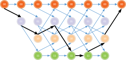
Fig. 6: An illustration of the VA trellis corresponding to the given input sequence {1011100}, where the data in the circles represent the states, the arrows represent all the possible paths, while the black bold arrows represent the survivor path having covered all the states. The survivor path is obtained in accordance with the selection criteria of VA.

Upon employing the principle of reduced-state trellis detection [41], a survivor path can be constructed in the MSDD trellis diagram based on VA. In particular, the computational complexity of the likelihood function (43) can be specified with a fixed memory depth of $L$ $(L\leq M)$, which is related to the range of $L$ and is a key design parameter determining the computational complexity. In order to make the VA applicable to MSDD, we attempt to construct a simplified expression of GLRT-MSDD, whose expression $\Lambda\left(\{y_{q}(t)\}_{q=1}^{Q}|\mathbb{U}\right)$ is approximated as

$$\begin{split}&\Gamma\left(\{y_{q}(t)\}_{q=1}^{Q}|\mathbb{U}\right)=\sum\limits_{i^{\prime}=1}^{M}\sum\limits_{l=\mathrm{max}\{0,i^{\prime}-L\}}^{i^{\prime}-1}\\ &\mathrm{Tr}\left(\left(\prod_{v=-i^{\prime}+1}^{-l}\mathbf{{\tilde{U}}}_{i+v}\right)\left(\sum\limits_{q=1}^{Q}\mathbf{Y}^{q}_{i-i^{\prime},l-i^{\prime}}\right)\right).\end{split}$$ (45)

In (45), the number of addends indexed by $l$ entails a maximum of $L$ instead of $i^{\prime}$. Thus, the approximate expression $\Gamma\left(\{y_{q}(t)\}_{q=1}^{Q}|\mathbb{U}\right)$ for MSDD is constrained by a fixed memory depth $L$, which facilitates the VA implementation. Let us set $\mathbf{{\tilde{U}}}_{i}^{(L)}\triangleq[\mathbf{\tilde{U}}_{i-L},\cdots,\mathbf{\tilde{U}}_{i}]^{\mathrm{T}}$, then (45) is rewritten as

$$\Gamma\left(\{y_{q}(t)\}_{q=1}^{Q}|\mathbf{{\tilde{U}}}_{i}^{M}\right)=\sum\limits_{i^{\prime}=1}^{M}\lambda_{i^{\prime}}(\mathbf{{\tilde{U}}}_{i-1}^{(L-1)},\mathbf{{\tilde{U}}}_{i}),$$ (46)

where we have

$$\begin{split}&\lambda_{i^{\prime}}(\mathbf{{\tilde{U}}}_{i-1}^{(L-1)},\mathbf{{\tilde{U}}}_{i})\triangleq\\ &\sum\limits_{l=\mathrm{max}\{0,i^{\prime}-L\}}^{i^{\prime}-1}\mathrm{Tr}\left(\left(\prod_{v=-i^{\prime}+1}^{-l}\mathbf{{\tilde{U}}}_{i+v}\right)\left(\sum\limits_{q=1}^{Q}\mathbf{Y}^{q}_{i-i^{\prime},l-i^{\prime}}\right)\right).\end{split}$$ (47)

Note that with a trellis representation, (47) stands for the branch metric at the $i^{\prime}$th stage in a trellis diagram, and it depends on the trellis $\mathbf{{\tilde{U}}}_{i}^{(L)}$ only. With $J_{i^{\prime}}(\mathbf{{\tilde{U}}}_{i}^{M})$ denoting the accumulated metric at the $i^{\prime}$th stage, it is plausible that the accumulated metric until the current stage can be formulated as the sum of that at the previous stage plus the current branch metric. More explicitly, we have

$$J_{i^{\prime}}(\mathbf{{\tilde{U}}}_{i}^{M})=J_{i^{\prime}-1}(\mathbf{{\tilde{U}}}_{i-1}^{M-1})+\lambda_{i^{\prime}}(\mathbf{{\tilde{U}}}_{i-1}^{(L-1)},\mathbf{{\tilde{U}}}_{i}),$$ (48)

which is an equivalent formulation to (45). As a beneficial result, the VA-HMSDD has been constructed. According to (47) and (48), the sequence of states corresponding to the survivor path yields the maximum value of the accumulated metric and uniquely defines the winning sequence of trellis state transitions from the first stage to the last one. As a result, the transmitted symbol sequence can be decided. Let us consider the given input sequence {1011100} as an example. Specifically, in Fig. 6 the hard-decision VA trellis is plotted, where the data in the circles represent the states, the arrows represent all the possible paths, while the black bold arrows represent the survivor path states. The survivor path is obtained in accordance with the selection criteria of VA. For the sake of clarity, the detailed procedure of the VA-HMSDD is specified in Table II. Note that the computational complexity of VA-HMSDD is fixed due to a given memory depth of $L$. This fulfills our goal of reducing the complexity of the conventional GLRT-MSDD, because we have $L\leq M$. Moreover, the proposed VA-HMSDD achieves the same detection performance as the GLRT-MSDD when $L=M$. In particular, when $M=1$, the complexity of the GLRT-MSDD cannot be simplified with the VA-HMSDD. In order to further enhance the detection performance of VA-HMSDD, in the next subsection, we develop a VA-SMSDD scheme, which is obtained by extending the trellis-based detection philosophy to the DSTBC aided UWB-IR systems.

Table II: Algorithm 2: The implementation of VA-HMSDD

Step 1)	Start from the initial state, and set $J_{0}=0$;
Step 2)	Set $\lambda_{1}(\mathbf{{\tilde{U}}}_{1})=\mathbf{Y}_{0,1}\mathbf{{\tilde{U}}}_{1}$, and update the accumulated function
	using $J_{1}(\mathbf{{\tilde{U}}}_{1})=J_{0}+\lambda_{1}(\mathbf{{\tilde{U}}}_{1})=\mathbf{Y}_{0,1}\mathbf{{\tilde{U}}}_{1}$;
Step 3)	Set $\lambda_{2}(\mathbf{{\tilde{U}}}_{1},\mathbf{{\tilde{U}}}_{2})=\mathbf{Y}_{1,2}\mathbf{{\tilde{U}}}_{2}+\mathbf{Y}_{0,2}\mathbf{{\tilde{U}}}_{1}\mathbf{{\tilde{U}}}_{2}$ and update the
	accumulated function for VA-HMSDD using
	$J_{2}(\mathbf{{\tilde{U}}}_{2})=J_{1}(\mathbf{{\tilde{U}}}_{1})+\lambda_{2}(\mathbf{{\tilde{U}}}_{1},\mathbf{{\tilde{U}}}_{2})$
	$=\mathbf{Y}_{0,1}\mathbf{{\tilde{U}}}_{1}+\mathbf{Y}_{1,2}\mathbf{{\tilde{U}}}_{2}+$ $\mathbf{Y}_{0,2}\mathbf{{\tilde{U}}}_{1}\mathbf{{\tilde{U}}}_{2}$;
Step $\cdots$
Step $M$)	Set and update the accumulated function using
	$\Gamma\left(\{y_{q}(t)\}_{q=1}^{Q}|\mathbb{U}\right)=J_{M}(\mathbf{{\tilde{U}}}_{M})$
	$=J_{M-1}(\mathbf{{\tilde{U}}}_{i-1}^{{M-1}})+\lambda_{M}(\mathbf{{\tilde{U}}}_{i-1}^{(L-1)},\mathbf{{\tilde{U}}}_{M})$.

IV-C Viterbi Algorithm Based Soft-Decision MSDD

The accumulated metric of (46) is related to the current input information symbol and the input information symbols of the previous stages. Consequently, the accumulated metric can be implemented on the trellis diagram. Upon invoking some mathematical manipulations concerning (46), we can explicitly formulate the forward-and-backward branch metrics as

$$\lambda(\alpha_{i-1}\rightarrow\alpha_{i})=\sum\limits_{i^{\prime}=1}^{M}\lambda_{i^{\prime}}(\mathbf{{\tilde{U}}}_{i-L}^{(L-1)},\mathbf{{\tilde{U}}}_{i})$$ (49)

and

$$\lambda(\beta_{i+1}\rightarrow\beta_{i})=\sum\limits_{i^{\prime}=1}^{M}\lambda_{i^{\prime}}(\mathbf{{\tilde{U}}}_{i+L}^{(L-1)},\mathbf{{\tilde{U}}}_{i+1}),$$ (50)

respectively. Correspondingly, relying on the branch metrics, the forward-and-backward accumulated path metrics are given by

$$u_{\mathrm{forward}}(\alpha_{i})=\max\limits_{\{\alpha_{i-1}\}}\{u_{\mathrm{forward}}(\alpha_{i-1})+\lambda(\alpha_{i-1}\rightarrow\alpha_{i})\}$$ (51)

and

$$u_{\mathrm{backward}}(\beta_{i})=\max\limits_{\{\beta_{i+1}\}}\{u_{\mathrm{backward}}(\beta_{i+1})+\lambda(\beta_{i+1}\rightarrow\beta_{i})\},$$ (52)

respectively. Based on (51) and (52), the VA-SMSDD is expressed as

$$\begin{split}\iota(d_{i}(k))&=\sum\limits_{(s^{\prime}\rightarrow s):d_{i}(k)=1}\{u_{\mathrm{forward}}(\alpha_{i})+u_{\mathrm{backward}}(\beta_{i})\}\\ &-\sum\limits_{(s^{\prime}\rightarrow s):d_{i}(k)=0}\{u_{\mathrm{fordward}}(\alpha_{i})+u_{\mathrm{backward}}(\beta_{i})\}.\end{split}$$ (53)

According to the expression $\iota(d_{i}(k))$, the channel decoder makes the decision as follows. If $\iota(d_{i}(k))\geq 0$, then $\hat{d}_{i}(k)=1$; otherwise, $\hat{d}_{i}(k)=0$. The proposed VA-SMSDD can be integrated into an IDD receiver when the a priori probabilities are taken into account in the detection process. As a result, in the $r$th iteration between the detector and the channel decoder, the accumulated path metrics of (51) and (52) are modified as

$$\begin{split}&u_{\mathrm{forward}}^{(r)}(\alpha_{i})=\max\limits_{\{\alpha_{i-1}\}}\{u_{\mathrm{forward}}^{(r)}(\alpha_{i-1})\\ &+\lambda(\alpha_{i-1}\rightarrow\alpha_{i})+\mathrm{ln}(\mathrm{Pr}^{(r-1)}(\alpha_{i-1}))\}\end{split}$$ (54)

and

$$\begin{split}&u_{\mathrm{backward}}^{(r)}(\beta_{i})=\max\limits_{\{\beta_{i+1}\}}\{u_{\mathrm{backward}}^{(r)}(\beta_{i+1})\\ &+\lambda(\beta_{i+1}\rightarrow\beta_{i})+\mathrm{ln}(\mathrm{Pr}^{(r-1)}(\beta_{i+1}))\},\end{split}$$ (55)

respectively, where $\mathrm{Pr}^{(r-1)}(\cdot)$ is the a priori probability gleaned from the channel decoder in the previous iteration.

Remark 5: By extending the trellis-based detection philosophy, the iterative VA-SMSDD is obtained, where the a priori probabilities are incorporated into the IDD process for achieving a more competitive performance than that of VA-HMSDD. Explicitly, the VA-SMSDD employs (53), which facilitates more reliable detection than the VA-HMSDD using (48).

Table III: Computational Complexity Comparisons of Four MSDD Algorithms.

Schemes

Computational Complexity

GLRT-MSDD	$O[(M+1)\cdot(2^{M})]$
VA-HMSDD	$O[(L+1)\cdot(2^{L})]$
BP-MSDD	$O[M\cdot(M+1)\cdot 2^{M}]$
VA-SMSDD	$O[M\cdot(L+1)\cdot 2^{L}]$

V Computational Complexity Analysis

In this section, the computational complexity of the conventional hard-decision GLRT-MSDD, of the VA-HMSDD, of the BP-MSDD and of the VA-SMSDD are compared.

Firstly, the complexity of the conventional GLRT-MSDD with hard-decision is analyzed. The lattice structure in (43) results in an exhaustive evaluation of all cross-correlation combinations. Then, the hard-decision GLRT-MSDD can be implemented relying on (39). Therefore, in terms of the number of multiplications required, the GLRT-MSDD imposes a computational complexity of $O[(M+1)\cdot(2^{M})]$, i.e., it increases exponentially with the observation window size $M$. By comparison, for the VA-HMSDD, as seen from (47), only those cross-terms with a memory depth no more than $L$ are taken into account. Therefore, the complexity of the VA-HMSDD increases exponentially with the memory depth $L$. More specifically, the computational complexity of VA-HMSDD reduces to $O[(L+1)\cdot(2^{L})]$ in terms of the total multiplications required. Consequently, when $L$ gets larger, the detection performance of the VA-HMSDD becomes closer to that of the conventional hard-decision GLRT-MSDD. Similar conclusions are also valid for the soft-decision based BP-MSDD versus the VA-SMSDD.

Secondly, the complexity of the proposed BP-MSDD and VA-SMSDD is compared. Specifically, the expression of the BP-MSDD given in (LABEL:zui) imposes a computational complexity of $O[M\cdot(M+1)\cdot 2^{M}]$. This is practically applicable only when $M$ is small. In order to maintain an affordable complexity when $M$ increases, VA-SMSDD is additionally conceived, which strikes an appealing performance-versus-complexity tradeoff. The maximum affordable complexity can be imposed through a proper selection of the finite memory depth $L$. As a result, the computational complexity of VA-SMSDD is on the order of $O[M\cdot(L+1)\cdot 2^{L}]$, where $2^{L}$ is the number of trellis states in each stage. In other words, its complexity increases exponentially only with $L$, rather than with $M$. Therefore, both the VA-HMSDD and the VA-SMSDD enjoy a flexibility in striking specific performance-versus-complexity tradeoffs. In summary, BP-MSDD achieves the best BER performance at the expense of high complexity. By comparison, VA-SMSDD constitutes a low-complexity detector suffering minor performance loss. For clarity, the complexity comparisons of these four MSDD algorithms are summarized in Table III. It is observed that VA-HMSDD has a lower complexity than the conventional hard-decision GLRT-MSDD, while the complexity of VA-SMSDD sits between that of VA-HMSDD and that of BP-MSDD.

VI Simulation Results and Discussions

In this section, numerical simulations are conducted to validate the effectiveness of the proposed MSDD algorithms. In all the simulations, a DSTBC aided UWB-IR system is considered. The channel is generated based on the IEEE 802.15.3a CM2 model [34]. This multipath channel remains invariant during each symbol burst, but randomly varies from burst to burst [33]. The assumption of channel invariance during each symbol burst is reasonable, since each transmitted burst includes only tens of symbols. The monocycle waveform $\omega(t)$ employed is the normalized second derivative of a Gaussian function, i.e., $\omega(t)=[1-4\pi(t/T_{\mathrm{m}})^{2}]\mathrm{exp}[-2\pi(t/T_{\mathrm{m}})^{2}]$, where the pulse duration is $T_{\mathrm{m}}=0.287\mathrm{ns}$. In order to eliminate the intersymbol interference, the frame duration is chosen as $T_{\mathrm{f}}=80\mathrm{ns}$, so that we have $T_{\mathrm{f}}$ $>$ $T_{\mathrm{n}}$, where $T_{\mathrm{n}}=40\mathrm{ns}$, denotes the maximum excess delay of the channel. Furthermore, the thermal noise is modeled as a white Gaussian process, with the two-sided power spectral density being $N_{0}/2$. Firstly, the BER performance of the proposed BP-MSDD is evaluated in Fig.7 and Fig. 8, where either the number of receive antennas $Q$ or the observation window size $M$ varies. To obtain insights concerning practical implementation, VA-HMSDD is investigated under different values of the design parameter $L$ in Fig. 9. Furthermore, the BER performance of the iterative BP-MSDD and of the iterative VA-SMSDD is compared in Fig. 10. Finally, the computational complexity comparisons of the BP-MSDD, VA-SMSDD, GLRT-MSDD and VA-HMSDD are visualized in Fig. 11.

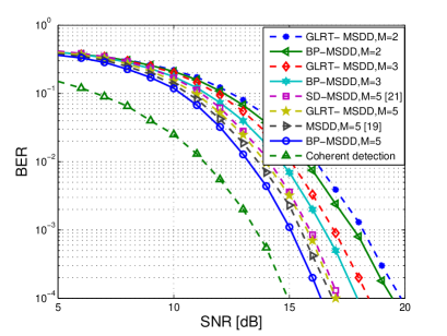
Fig. 7: BER performance comparisons of the coherent detector, the proposed BP-MSDD, the conventional GLRT-MSDD and the MSDDs proposed in [19] and [21]. $Q=1$, $M=2$, 3 and 5.

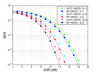
Fig. 8: BER performance comparisons of the proposed BP-MSDD and the conventional hard-decision GLRT-MSDD. $M=3$, $Q=1$, 2 and 3.

Test Scenario 1: This test scenario is devoted to demonstrating the effectiveness of the proposed BP-MSDD without considering the channel coding. Specifically, in Fig. 7 we illustrate the BER performance comparisons of the proposed BP-MSDD, the conventional GLRT-MSDD, and the MSDDs proposed in [19] and [21]. Moreover, a coherent rake receiver [42] with 12 fingers is also evaluated as the performance benchmark. The number of receive antennas is fixed to $Q=1$, while the observation window size is set to $M=2,3$ and 5, respectively. It is clear that BP-MSDD achieves a better BER performance than the hard-decision GLRT-MSDD, e.g., about 0.4$\mathrm{dB}$ gain is attained at the BER of $10^{-4}$ when $M=2$. In addition, this BER performance advantage becomes larger when $M$ increases. It can be seen that BP-MSDD outperforms the BCJR-based MSDDs of [19] when $M=5$. This is due to the more reliable information obtained by the BP-MSDD relying on the proposed AcR sampling and metric function than that obtained by the BCJR-based MSDD of [19]. Also, the BP-MSDD is superior to the MSDD of [21]. Although performance loss is observed in comparison with the coherent reception, the benefit of the proposed noncoherent BP-MSDD is still evident without channel estimation. Furthermore, the BER performance of the proposed BP-MSDD is investigated by varying the number of receive antennas $Q$. Specifically, in Fig. 8 the BER performance of BP-MSDD is plotted for the scenario where $M=3$, $Q=1$, 2 and 3, respectively. It is observed that the curves in Fig. 8 have similar trend to those of Fig. 7, and in Fig. 8 the proposed BP-MSDD always enjoys a performance improvement compared to the conventional hard-decision GLRT-MSDD, regardless of the specific values of $Q$. This is attributed to the advantage of the forward-and-backward message passing mechanism of the BP-MSDD.

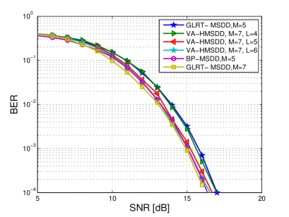
Fig. 9: BER performance comparisons of the proposed VA-HMSDD, the conventional hard-decision GLRT-MSDD, and the proposed BP-MSDD. The observation window size is $M=5$, 7, while the value of $L$ varies.

Test Scenario 2: Compared to the BP-MSDD and the conventional hard-decision GLRT-MSDD, the proposed VA-HMSDD represents a suboptimal reduced-complexity alternative, where the maximum affordable complexity is imposed through a proper selection of the VA memory depth $L$. In Fig. 9 we compare the BER performance of the conventional hard-decision GLRT-MSDD and of the proposed VA-HMSDD by setting the observation window size to $M=7$, and the VA memory depth to $L=4$, 5 and 6, respectively. It can be seen from Fig. 9 that there exists a performance gap between the conventional hard-decision GLRT-MSDD and the proposed VA-HMSDD when $L<M$. The difference in BER performance is due to the different decision metrics employed. The detection performance of VA-HMSDD is constrained by the memory depth $L$ for a given $M$, since $L$ determines the number of cross-terms in the approximating objective metric function of (45). By contrast, the conventional hard-decision GLRT-MSDD employs the exact objective metric function of (39), hence it achieves a better BER performance. In fact, VA-HMSDD is based on an equivalent reformulation of the MSDD criterion and it maintains the BER performance of the original MSDD when $M=L$. Interestingly, the low-complexity VA-HMSDD only incurs a small performance loss when $L$ is close to $M$, e.g., the VA-HMSDD with $L=6$ suffers a SNR penalty of about 0.2$\mathrm{dB}$ compared to the conventional hard-decision GLRT-MSDD with $M=7$. When the design parameter $L$ is increased, the detection performance of VA-HMSDD becomes closer to that of the original GLRT-MSDD. As expected, at the $\mathrm{BER}=10^{-4}$, compared with the case of $L=6$, VA-HMSDD with $L=3$ suffers a BER performance degradation of about 1$\mathrm{dB}$. It is worth noting that, when $M$ is large, the conventional hard-decision GLRT-MSDD is not applicable due to its unaffordable complexity. Yet, our VA-HMSDD can remain computationally practical when selecting a small $L$, despite a little BER performance degradation. Moreover, we consider the BER performance comparison of the BP-MSDD and the VA-HMSDD when their complexity are approximately equal. Fig. 9 demonstrates that when $M_{1}=5$ for BP-MSDD, $M_{2}=7$, $L=4$, 5 for VA-HMSDD, their complexity are close to each other. In this case, the BER performance of the BP-MSDD is slightly better than the VA-HMSDD.

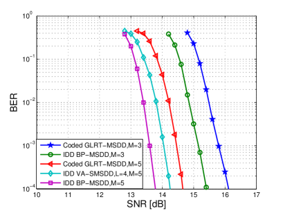
Fig. 10: BER performance comparisons of the coded GLRT-MSDD with $M=3$, 5, the IDD BP-MSDD with $M=3$, 5 and the IDD VA-SMSDD with $L=4$, $M=5$ for $Q=1$.

Test Scenario 3: In this test scenario, the BER performance of the iterative BP-MSDD, the iterative VA-SMSDD and the coded GLRT-MSDD without iteration are studied to reveal relevant insights into the IDD receiver design relying on the MSDD philosophy. In particular, the SISO BP-MSDD is specified by (LABEL:zui), and the low-complexity VA-SMSDD is based on the decision metric of (53). For fair comparison, all the receivers employ a rate-1/2 convolutional code [27], whose generator polynomial is (133, 171) in octal form and the constraint length is 7. For the iterative BP-MSDD and the iterative VA-SMSDD, four iterations are performed between the symbol detector and the channel decoder. It is observed from Fig. 10 that the BP-MSDD based IDD receiver enjoys an appealing BER performance advantage compared with the coded GLRT-MSDD. To better understand the effectiveness of the simplified VA criterion, the BER performance of the VA-SMSDD based IDD receiver is illustrated in Fig. 10 as well. It can be seen that there exists a small performance gap between the BP-MSDD based IDD receiver with $M=5$ and the VA-SMSDD based IDD receiver with $L=4$. This is because the BP-MSDD based IDD employs an exact objective metric function of (LABEL:zui), while the VA-SMSDD based IDD employs an approximate simplified function of (53).

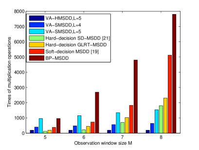
Fig. 11: Complexity comparisons of the BP-MSDD, the soft-decision MSDD in [19], the hard-decision GLRT-MSDD, the hard-decision SD-MSDD in [21], the VA-SMSDD and the VA-HMSDD against different observation window size $M$ and different VA memory depth $L$.

Test Scenario 4: To consolidate the computational complexity analysis provided in Section V, the computational complexity in terms of multiplication operation of the BP-MSDD, the soft-decision MSDD in [19], the hard-decision GLRT-MSDD, the hard-decision SD-MSDD in [21], the VA-SMSDD and the VA-HMSDD is illustrated in Fig. 11 against different observation window size $M$ and different VA memory depth $L$. It is observed that the VA-SMSDD exhibits a complexity reduction compared with the BP-MSDD, especially for a large value of $M$ and a small value of $L$. This is because the number of trellis states for the BP-MSDD increases exponentially with the observation window size $M$, which inevitably results in high computational complexity. In contrast to the BP-MSDD, the complexity of VA-SMSDD increases exponentially with the memory depth $L$, which satisfies $L\leq M$. Hence, a lower complexity can be obtained when selecting a small $L$ for the VA-SMSDD. It is also observed from Fig. 11 that the proposed VA-HMSDD enjoys a complexity reduction compared to the hard-decision GLRT-MSDD, regardless of the specific values of $M$; the complexity of the soft-decision MSDD in [19] is lower than the BP-MSDD, and the complexity of the hard-decision SD-MSDD in [21] is slightly lower than that of the hard-decision GLRT-MSDD.

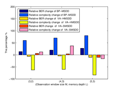
Fig. 12: BER performance and computational complexity comparisons of the BP-MSDD, VA-HMSDD, VA-SMSDD against the GLRT-MSDD in terms of relative percentage with different combinations of $(M,L)=(3,2)$, $(4,3)$ and $(5,3)$, respectively. The relative complexity and the relative BER performance are defined as $\frac{C_{\mathrm{CA}}-C_{\mathrm{GLRT}}}{C_{\mathrm{GLRT}}}\times 100\%$ and $\frac{B_{\mathrm{GLRT}}-B_{\mathrm{CA}}}{B_{\mathrm{GLRT}}}\times 100\%$, respectively.

In addition, the relative BER performance and computational complexity results under several different combinations of the parameter values $(M,L)$ are illustrated in Fig. 12. The positive percentage represents the BER performance improvement and the computational complexity increase compared to those of the benchmark GLRT-MSDD; meanwhile, negative percentage represents the BER performance loss and the computational complexity reduction compared to those of the benchmark GLRT-MSDD. The relative complexity and the relative BER performance are defined as $\frac{C_{\mathrm{CA}}-C_{\mathrm{GLRT}}}{C_{\mathrm{GLRT}}}\times 100\%$ and $\frac{B_{\mathrm{GLRT}}-B_{\mathrm{CA}}}{B_{\mathrm{GLRT}}}\times 100\%$, respectively, where $C_{\mathrm{CA}}$ and $B_{\mathrm{CA}}$ represent the complexity and the BER performance of the compared algorithm, respectively; while $C_{\mathrm{GLRT}}$ and $B_{\mathrm{GLRT}}$ are the complexity and the BER performance of the GLRT, respectively. From Fig. 12, we can see that for all the combinations of $(M,L)=(3,2)$, $(4,3)$ and $(5,3)$, the BER performance of the BP-MSDD is superior to that of the noncoherent GLRT-MSDD at the cost of increased computational complexity; by contrast, for these combinations of $(M,L)$ values, the VA-HMSDD imposes a reduced computational complexity at the expense of a small performance loss. Notably, the VA-SMSDD shows both positive and negative percentages under these combinations of (M, L) values, which indicates that the BER performance and the computational complexity of the VA-SMSDD are bounded by those of the BP-MSDD and the VA-HMSDD.

VII Conclusions

A fundamental BP-MSDD framework is proposed for efficiently calculating the a posteriori information of the symbols transmitted. The BP-MSDD achieves appealing performance by exploiting a trellis having a full number of states. Furthermore, to facilitate the practical implementations of the MSDD, the proposed BP-MSDD is reformulated from the perspective of LLR, where the likelihood of MSDD is simplified, and a low-complexity VA-HMSDD is derived with the aid of a trellis having a reduced number of states. Additionally, a soft-decision based VA-SMSDD is proposed, which achieves better performance than the hard-decision based VA-HMSDD. Both the BP-MSDD and the VA-SMSDD are capable of flexibly providing tradeoffs between the achievable performance and the computational complexity imposed. Finally, since both of the proposed BP-MSDD and VA-SMSDD are SISO algorithms, they are capable of substantially improving the receiver’s BER performance by invoking the IDD philosophy. Simulation results have demonstrated the effectiveness of the proposed algorithms in the illustrative context of DSTBC aided UWB-IR systems.

Chanfei Wang is now working towards the Ph.D. degree in information engineering from Beijing University of Posts and Telecommunications (BUPT), Beijing, China. Her research interests focus on signal processing techniques in ultra-wideband wireless communications.

Tiejun Lv (M’08-SM’12) received the M.S. and Ph.D. degrees in electronic engineering from the University of Electronic Science and Technology of China (UESTC), Chengdu, China, in 1997 and 2000, respectively. From January 2001 to January 2003, he was a Postdoctoral Fellow with Tsinghua University, Beijing, China. In 2005, he became a Full Professor with the School of Information and Communication Engineering, Beijing University of Posts and Telecommunications (BUPT). From September 2008 to March 2009, he was a Visiting Professor with the Department of Electrical Engineering, Stanford University, Stanford, CA, USA. He is the author of more than 200 published technical papers on the physical layer of wireless mobile communications. His current research interests include signal processing, communications theory and networking. Dr. Lv is also a Senior Member of the Chinese Electronics Association. He was the recipient of the Program for New Century Excellent Talents in University Award from the Ministry of Education, China, in 2006. He received the Nature Science Award in the Ministry of Education of China for the hierarchical cooperative communication theory and technologies in 2015.

Hui Gao (S’10-M’13-SM’16) received his B. Eng. degree in Information Engineering and Ph.D. degree in Signal and Information Processing from Beijing University of Posts and Telecommunications (BUPT), Beijing, China, in July 2007 and July 2012, respectively. From May 2009 to June 2012, he also served as a research assistant for the Wireless and Mobile Communications Technology R and D Center, Tsinghua University, Beijing, China. From Apr. 2012 to June 2012, he visited Singapore University of Technology and Design (SUTD), Singapore, as a research assistant. From July 2012 to Feb. 2014, he was a Postdoc Researcher with SUTD. He is now with the School of Information and Communication Engineering, Beijing University of Posts and Telecommunications (BUPT), as an assistant professor. His research interests include massive MIMO systems, cooperative communications, ultra-wideband wireless communications.

Shaoshi Yang (S’09-M’13) received his B.Eng. degree in Information Engineering from Beijing University of Posts and Telecommunications (BUPT), Beijing, China in Jul. 2006, his first Ph.D. degree in Electronics and Electrical Engineering from University of Southampton, U.K. in Dec. 2013, and his second Ph.D. degree in Signal and Information Processing from BUPT in Mar. 2014. He is now working as a Postdoctoral Research Fellow in University of Southampton, U.K. From November 2008 to February 2009, he was an Intern Research Fellow with the Communications Technology Lab (CTL), Intel Labs, Beijing, China, where he focused on Channel Quality Indicator Channel (CQICH) design for mobile WiMAX (802.16m) standard. His research interests include MIMO signal processing, green radio, heterogeneous networks, cross-layer interference management, convex optimization and its applications. He has published in excess of 30 research papers on IEEE journals. Shaoshi has received a number of academic and research awards, including the prestigious Dean’s Award for Early Career Research Excellence at University of Southampton, the PMC-Sierra Telecommunications Technology Paper Award at BUPT, the Electronics and Computer Science (ECS) Scholarship of University of Southampton, and the Best PhD Thesis Award of BUPT. He is a member of IEEE/IET, and a junior member of Isaac Newton Institute for Mathematical Sciences, Cambridge University, U.K. He also serves as a TPC member of several major IEEE conferences, including IEEE ICC, GLOBECOM, VTC, WCNC, PIMRC, ICCVE, HPCC, and as a Guest Associate Editor of IEEE Journal on Selected Areas in Communications. (http://sites.google.com/site/shaoshiyang/).

References

- [1] S. Yang and L. Hanzo, “Fifty years of MIMO detection: The road to large-scale MIMOs,” IEEE Commun. Surveys Tuts., vol. 17, no. 4, pp. 1941–1988, 4th Quart. 2015.
- [2] G. Foschini, L. Greenstein, and G. Vannucci, “Noncoherent detection of coherent lightwave signals corrupted by phase noise,” IEEE Trans. Commun., vol. 36, no. 3, pp. 306–314, Mar. 1998.
- [3] M. Win and R. Scholtz, “On the energy capture of ultrawide bandwidth signals in dense multipath environments,” IEEE Commun. Lett., vol. 2, no. 9, pp. 245–247, Sep. 1998.
- [4] M. Simon and M. Alouini, “A unified approach to the probability of error for noncoherent and differentially coherent modulations over generalized fading channels,” IEEE Trans. Commun., vol. 46, no. 12, pp. 1625–1638, Dec. 1998.
- [5] H. Leib and S. Pasupathy, “The phase of a vector perturbed by Gaussian noise and differentially coherent receivers,” IEEE Trans. Inf. Theory., vol. 34, no. 6, pp. 1491–1501, Nov. 1988.
- [6] P. Ho and D. Fung, “Error performance of multiple symbol differential detection of PSK signals transmitted over correlated Rayleigh fading channels,” in Proc. IEEE Int. Conf. Commun. (ICC 1991), Denver, CO, USA, Jun. 1991, pp. 23–26.
- [7] F. Adachi and M. Sawahashi, “Decision feedback multiple-symbol differential detection for M-ary DPSK,” Electron. Lett., vol. 29, no. 15, pp. 1385–1387, Jul. 1993.
- [8] A. Abrardo, G. Benelli, G. Cau, “Multiple-symbol differential detection of GMSK for mobile communications,” IEEE Trans. Veh. Technol., vol. 44, no. 3, pp. 379–390, Aug. 1995.
- [9] L. Lampe, R. Schober, V. Pauli, and C. Windpassinger, “Multiple-symbol differential sphere decoding,” IEEE Trans. Commun., vol. 53, no. 12, pp. 1981–1985, Dec. 2005.
- [10] D. Divsalar and M. Simon, “Multiple symbol differential detection of MPSK,” IEEE Trans. Commun., vol. 38, no. 3, pp. 300–308, Mar. 1990.
- [11] V. Lottici and Z. Tian, “Multiple symbol differential detection for UWB communications,” IEEE Trans. Wireless Commun., vol. 7, no. 5, pp. 1656–1666, May 2008.
- [12] D. Warrier and U. Madhow, “Spectrally efficient noncoherent communication,” IEEE Trans. Inf. Theory., vol. 48, no. 3, pp. 651–668, Mar. 2002.
- [13] V. Tarokh, H. Jafarkhani, and A. R. Calderbank, “Space-time block codes from orthogonal designs,” IEEE Trans. Inf. Theory., vol. 45, no. 5, pp. 1456–1467, Jul. 1999.
- [14] V. Tarokh and H. Jafarkhani, “A differential detection scheme for transmit diversity,” IEEE J. Sel. Areas Commun., vol. 18, no. 7, pp. 1169–1174, Jul. 2000.
- [15] P. Fan, “Multiple-symbol detection for transmit diversity with differential encoding scheme,” IEEE Trans. Consum. Electron., vol. 47, no. 1, pp. 96–100, Feb. 2001.
- [16] T. Wang, T. Lv, H. Gao, and Y. Lu, “BER analysis of decision-feedback multiple symbol detection in non-coherent MIMO ultra-wideband systems,” IEEE Trans. Veh. Technol., vol. 62, no. 9, pp. 4684–4690, Nov. 2013.
- [17] T. Wang, T. Lv, and H. Gao, “Sphere decoding based multiple symbol detection for differential space-time block coded ultra-wideband systems,” IEEE Commun. Lett., vol. 15, no. 3, pp. 269–271, Mar. 2011.
- [18] R. Fischer, L. Lampe, and S. Weinfurtner, “Coded modulation for noncoherent reception with application to OFDM,” IEEE Trans. Veh. Technol., vol. 50, no. 4, pp. 910–919, Jul. 2001.
- [19] P. Vanichchanunt, P. Sangwongngam, S. Nakpeerayuth, and L. Wuttisittikulkij, “Iterative multiple symbol differential detection for Turbo coded differential unitary space-time modulation,” Journal of Communication and Networks, vol. 10, no. 1, pp. 44–54, Mar. 2008.
- [20] I. Marsland and P. Mathiopoulos, “On the performance of iterative noncoherent detection of coded MPSK signals,” IEEE Trans. Commun., vol. 48, no. 4, pp. 588–596, Apr. 2000.
- [21] V. Pauli, L. Lampe, and R. Schober, ““Turbo DPSK” using soft multiple symbol differential sphere decoding,” IEEE Trans. Inf. Theory., vol. 52, no. 4, pp. 1385–1398, Apr. 2006.
- [22] B. Hochwald and S. ten Brink, “Achieving near-capacity on a multiple-antenna channel,” IEEE Trans. Commun., vol. 51, no. 3, pp. 389–399, Mar. 2003.
- [23] C. Berrou, A. Glavieux, and P. Thitimajshima, “Near Shannon limit error-correcting coding and decoding: Turbo Codes,” in Proc. IEEE Int. Conf. Commun. (ICC 1993), Geneva, Switzerland, May 1993, pp. 1064-1070.
- [24] S. Yang, L. Wang, T. Lv, and L. Hanzo, “Approximate Bayesian probabilistic-data-association-aided iterative detection for MIMO systems using arbitrary M-ary modulation,” IEEE Trans. Veh. Technol., vol. 62, no. 3, pp. 1228–1240, Mar. 2013.
- [25] S. Yang, T. Lv, R. Maunder, and L. Hanzo, “From nominal to true a posteriori probabilities: An exact Bayesian theorem based probabilistic data association approach for iterative MIMO detection and decoding,” IEEE Trans. Commun., vol. 61, no. 7, pp. 2782–2793, Jul. 2013.
- [26] F. Kschischang, B. Frey, and H. Loeliger, “Factor graphs and the sum-product algorithm,” IEEE Trans. Inf. Theory., vol. 47, no. 2, pp. 498–519, Feb. 2001.
- [27] M. Fossorier, S. Lin, and D. Costello, “On the weight distribution of terminated convolutional codes,” IEEE Trans. Inf. Theory., vol. 45, no. 5, pp. 1646–1648, Jul. 1999.
- [28] M. Fossorier, M. Mihaljevic, and H. Imai, “Reduced complexity iterative decoding of low density parity check codes based on belief propagation,” IEEE Trans. Commun., vol. 47, no. 5, pp. 673–680, May 1999.
- [29] L. Bahl, J. Cocke, F. Jelinek, and J. Raviv, “Optimal decoding of linear codes for minimizing symbol error rate,” IEEE Trans. Inf. Theory., vol. 20, no. 2, pp. 284–287, Mar. 1974.
- [30] T. Wang, T. Lv, H. Gao, and S. Zhang (2015, Apr. 5). “Joint multiple symbol differential detection and channel decoding for noncoherent UWB impulse radio by belief propagation,” [Online]. Available: http://arxiv.org/abs/1504.01100.
- [31] H. Loeliger. “An introduction to factor graphs,” IEEE Signal Processing Mag., vol. 21, no. 1, pp. 28–41, Jan. 2004.
- [32] H. Niu, M. Shen, J. A. Ritcey, and H. Liu, “A factor graph approach to iterative channel estimation and LDPC decoding over fading channels,” IEEE Trans. Wireless Commun., vol. 4, no. 4, pp. 1345-1350, Jul. 2005.
- [33] M. Z. Win and R. A. Scholtz, “Ultra-wide bandwidth time-hopping spread-spectrum impulse radio for wireless multiple-access communications,” IEEE Trans. Commun., vol. 48, no. 4, pp. 679–689, Apr. 2000.
- [34] Q. Zhang and C. Ng, “DSTBC impulse radios with autocorrelation receiver in ISI-free UWB channels,” IEEE Trans. Wireless Commun., vol. 7, no. 3, pp. 806–811, Mar. 2008.
- [35] T. Quek and M. Win, “Analysis of UWB transmitted-reference communication systems in dense multipath channels,” IEEE J. Sel. Areas Commun., vol. 23, no. 9, pp. 1863–1874, Sep. 2005.
- [36] Y. S. Shmaliy, “On the multivariate conditional probability density of a vector perturbed by Gaussian noise,” IEEE Trans. Inf. Theory., vol. 53, no. 12, pp. 4792–4797, Dec. 2007.
- [37] R. W. Chang and J. C. Hancock, “On receiver structures for channels having memory,” IEEE Trans. Inf. Theory., vol. 12, no. 4, pp. 463–468, Oct. 1966.
- [38] C. Tan and N. Beaulieu, “On first-order Markov modeling for the Rayleigh fading channel,” IEEE Trans. Commun., vol. 48, no. 12, pp. 2032–2040, Dec. 2000.
- [39] Y. Ephraim and N. Merhav, “Hidden Markov processes,” IEEE Trans. Inf. Theory., vol. 48, no. 6, pp. 1518–1569, Jun. 2002.
- [40] Y. Li, C. N. Georghiades, and G. Huang, “Iterative maximum-likelihood sequence estimation for space-time coded systems,” IEEE Trans. Commun., vol. 49, no. 6, pp. 948–951, Jun. 2001.
- [41] G. Rajan and B. Rajan, “Algebraic distributed differential space-time codes with low decoding complexity,” IEEE Trans. Wireless Commun., vol. 7, no. 10, pp. 3962–3971, Oct. 2008.
- [42] L. Yang and G. Giannakis, “Analog space-time coding for multiantenna ultra-wideband transmissions,” IEEE Trans. Commun., vol. 52, no. 3, pp. 507–517, Mar. 2004.