Improving Quality of Hierarchical
Clustering for Large Data Series
Manuel R. Ciosici
 
Master’s Thesis, Computer Science
December 2015
Advisors: Ira Assent and Sean Chester

Abstract

Brown clustering is a hard, hierarchical, bottom-up clustering of words in a vocabulary. Words are assigned to clusters based on their usage pattern in a given corpus. The resulting clusters and hierarchical structure can be used in constructing class-based language models and for generating features to be used in natural language processing (NLP) tasks. Because of its high computational cost, the most-used version of Brown clustering is a greedy algorithm that uses a window to restrict its search space. Like other clustering algorithms, Brown clustering finds a sub-optimal, but nonetheless effective, mapping of words to clusters. Because of its ability to produce high-quality, human-understandable cluster, Brown clustering has seen high uptake the NLP research community where it is used in the preprocessing and feature generation steps.

Very little research has been done towards improving the quality of Brown clusters, despite the greedy and heuristic nature of the algorithm. The approaches tried so far have focused on: studying the effect of the initialisation in a similar algorithm (the Exchange Algorithm); tuning the parameters used to define the desired number of clusters and the behaviour of the algorithm; and including a separate parameter to differentiate the window from the desired number of clusters. However, some of these approaches have not yielded significant improvements in cluster quality.

In this thesis, a close analysis of the Brown algorithm is provided, revealing important under-specifications and weaknesses in the original algorithm. These have serious effects on cluster quality and reproducibility of research using Brown clustering. In the second part of the thesis, two modifications are proposed. Together, these improve the way in which the heuristics are actually applied, improve the quality of Brown clusters and provide consistent results. Finally, a thorough evaluation is performed, considering both the optimization criterion of Brown clustering and the performance of the resulting class-based language models.

Chapter 1 Introduction

A wide variety of computer applications, such as speech recognition, spell checking, and predictive text (assisting text input by suggesting next most likely words) and machine translation, require computer systems that have knowledge of human languages. More specifically, given half a sentence or query, they require the ability to predict what word might come next.

Human-spoken languages have human-understandable grammars to help people learn the language and agree on how it should be written and spoken. However, the grammars used by humans to learn languages are not suited for computers. They make use of what we call common sense, which computers severely lack. This becomes especially problematic for computers where natural language is unclear and common sense is necessary for a proper understanding. For example, a formulation such as “Was good god corroded” might seem to be allowed in English since word order respects the Grammar of English. Common sense, though, tells us that because the sentence doesn’t make sense, it is most likely an error. A computer would not be able to tell this as there is no way to express the relationships between every possible noun and every possible adjective in English.

Computer scientists have made various efforts to develop grammars that computers can understand. Context Free Grammars are among the most powerful tools trying to address this issue, and were a foundation stone in developing today’s advanced programming languages. Context Free Languages are formed of a series of terminal states, representing the smallest elements of a language (i.e. words), a list of non-terminal states and rules for how to decompose the non-terminal states either into more non-terminal states, or into terminal states. By using this system one can describe what sort of constructs can appear in contrived languages, such as programming languages. However, Context Free Grammars do not apply well to natural languages for various reasons, such as language inconsistencies, which we humans are quite happy with. The limitations of Context Free Grammars have led researchers to explore ways to derive models of human languages using automated learning techniques. Statistical Language Models are a class of techniques probabilistically modeling the use of a language. The models normally learn by analyzing large corpora of text and inferring what words are most likely to follow which other words. For example, given the construct How are, it is quite easy to imagine that the next most likely word is from the set {you, they, the}, rather than {antelopes, dwarfs, boxes}. In normal use of English the questions How are you? and How are the … are far more common than questions starting with How are antelopes… Statistical language models are especially interesting because they generally require no linguistic knowledge. A good statistical language modeling algorithm can be just as easily applied to French as it can to English; all it needs is a sufficiently large corpus of French text from which to learn.

Statistical language models work because they learn to estimate the flow of words in a specific language based on its use. The models make some assumptions about the structure of language and learn from the usage observed in a corpus of the language. For example, the class of statistical language models dealt with in this thesis makes the assumption that the probability of the next word depends only on the previous $n$ words, where $n$ is generally a small number like 1 or 3. This assumption can be easily proven not to hold even with simple sentences: In the sentence, The defendant, said the prosecutor, is not guilty, the word is is obviously dependent on the second word in the sentence, which is at a distance of 4 words, so any model assuming that less than the 4 previous words can influence the next word will not be able to model the sentence properly. While such assumptions can easily be proven wrong, models based on them work quite well in practice. Unfortunately, not all terms in any language are used with the same frequency. Low usage of some constructs in a corpus creates difficulties for models trying to learn to estimate language usage. For example, because this thesis is not on a topic in Biology, nouns denoting animals are used sparingly which will cause language models trained on the text of this thesis to have problems predicting what words should follow dog or elephant, but will give the language model a pretty good idea that after the word language, we should see the word model. The problem of reliably predicting words from a corpus is caused by data sparsity.

The data sparsity problem manifests itself through brittle models. By brittle, we mean that a model doesn’t generalize well. For example, a model trained on texts used in news stories and which performs quite well when asked to predict text written in the style of a news story, often turns out to perform badly when asked to assist in predicting email content. Class-based models attempt to improve generalization of language models at the expense of accuracy. Word classes (or word clusters) are groupings of words, such that each group contains words that have similar usage in the target language. By grouping words together into classes (or clusters), class-based language models can use the occurrences of all words in a class to derive a better estimate of how often the class occurs. Class-based language models are less accurate, as they are less expressive than their non-class-based counterparts. They are also crucially dependent on algorithms that create good word classes. It could be highly rewarding for all the applications mentioned earlier in this chapter to develop algorithms that are better at assigning words to word clusters (word classes).

Brown clustering is an assignment of words from a vocabulary $V$ to clusters (word equivalence classes) in a hierarchical clustering. A hierarchical clustering is a structure similar to a pyramid. Each level contains clusters that represent the merging of two clusters on a lower level. The lowest level is formed of clusters containing a single word. Word assignment to clusters is based on word probability distribution within a corpus of text consisting of all words in the vocabulary $V$. Brown clustering is a hard clustering, meaning that every word can only be part of a single cluster at every level. Brown clustering can be used as part of a language model, in tasks such as spell checking and speech recognition, or as a source of text features in tasks such as named entity recognition or machine translation.

The Brown clustering algorithm takes as input a corpus of text composed of words $w_{1}$, $w_{2}$, $w_{3}$, …, $w_{n}$ and a parameter $C$ for the number of clusters into which the words should be grouped. A bottom-up approach is used to perform hierarchical clustering. Each word $w_{i}$ is first allocated to its own cluster $C_{1}(i)$, after which clusters are iteratively merged, two at a time, until only one cluster remains, in effect producing the hierarchical clustering. The clusters $C_{k}(i)$ and $C_{k}(j)$ to be merged at step $k+1$ are chosen from among the clusters resulting from step $k$ such as to minimize an information theoretical measure defined in one of the following chapters. For example, the words Monday and Tuesday, which are generally used in the same way, could be merged into a single cluster.

1.1 Contributions

Brown clustering has seen wide uptake in the research community and is used in current state-of-the-art algorithms for Named Entity Recognition and Part of Speech tagging, as shown later, in Section 2.3.2. As shown by [7], Brown clustering produces nice word clusters. However, there is very little research on whether those clusters can be dramatically improved. Besides this, there is a lot of ambiguity in the definition of Brown clustering which leads to implementations acting more like interpretations. In this thesis I challenge the ambiguity in Brown clustering’s definition and show how it leads to unpredictable results. I also challenge some generally held assumptions on the quality of windowed Brown clustering against non-windowed Brown clustering. Finally, I propose two modifications to the windowed Brown clustering ALLSAME and RESORT that aim to make results repeatable and improve the quality of resulting clusters

1.2 Overview of following chapters

In Chapter 2, I provide some background on Brown clustering, I motivate the use of language models and cover the differences between class-based language models and regular language models. I also briefly present a few applications of Brown clustering. I cover related research on Brown clustering in Chapter 3, especially the limited work on improving the cluster quality. Chapter 4 contains a thorough analysis of the Brown algorithm illustrating weaknesses in the algorithm’s original specification. I propose two modifications to the windowed Brown clustering algorithm in Chapter 5, followed by thorough empirical evaluation in Chapter 6. Finally, Chapter 7 concludes this thesis and presents a few directions for future work on Brown clustering.

Chapter 2 Background

This chapter will provide a short introduction to statistical language models: what they are and their various kinds (Section 2.1). The chapter will then introduce class-based language models (Section 2.2), what issues they attempt to address. Section 2.3 will present various applications of statistical language models and of Brown clustering.

2.1 Statistical language models

A statistical language model ([3, 7, 26]) is an application of Markov Models to natural languages. A Markov Model is a stochastic model used to model the sequences of transitions in a system of states. When Markov Models are used in language models the various words of a vocabulary are considered to be the states. Transitions between states are sequences of two words that can appear consecutively in the language. Language models attempt to estimate the transition probabilities between words in a vocabulary. A Markov Model assumes the Markov Property which requires that future states depend only on the present state. Let $S$ be a sequence of text from a language $L$, where $S=w_{1},w_{2},\dots,w_{n}$ and $w_{k}$ denotes the $k$’th word in $S$. A bigram language model for $L$ that assumes the Markov Property will assume that the next word ($w_{k}$) to appear in $S$ depends only on the current word ($w_{k-1}$). Formally:

$$p(w_{k}|w_{1},w_{2},\dots w_{k-1})=p(w_{k}|w_{k-1})$$ (2.1)

This kind of Markov Model is called a first order Markov Model. The model can be extended so that the probability of word $w_{k}$ depends both on $w_{k-1}$ and $w_{k-2}$, thus creating a second order Markov Model:

$$p(w_{k}|w_{1},w_{2},\dots w_{k-1})=p(w_{k}|w_{k-1},w_{k-2})$$ (2.2)

The second order Markov Model uses tri-grams (groups of tree words appearing consecutively). This is opposed to the first order Markov model which uses bi-grams (pairs of words appears after each other in the corpus). We can generalize to higher order Markov models by using n-grams:

$$p(w_{k})=\displaystyle\prod_{i=1}^{n}p(w_{i}|w_{1}\dots w_{i-1})$$ (2.3)

It is easy to find examples of real-world language use where the Markov Property doesn’t hold. In the sentence: They, Angela and Martin, are always late, the word are is determined by the first word in the sentence (They), which 4 words away. It is first with a fourth order Markov Model that we would be able to model this dependence. However, one could make the iteration of names longer, making it practically impossible to use very high order Markov Models. Even though these limitations exist in Markov Models, lower order models still manage to do a good job at capturing language usage, which is why they are widely used.

Markov models are derived by computing probabilities based on a given sample of observations. In the case of language models, the sample of observations is a corpus of text. The vocabulary size defines the number of parameters to be estimated. For a first order Markov model over a vocabulary $V$ of size $|V|$ there are $|V|^{2}$ parameters (i.e., transitions) to estimate. We need $|V|$ probabilities estimated for each of the $|V|$ words in the vocabulary. For a second order Markov model the number of parameters becomes $|V|^{3}$. A language model built even for a small number of the words in a language must estimate a large number of parameters. For example, a model on a vocabulary of size $20\ 000$ must estimate $400\ 000\ 000$ parameters when using a bi-gram model and $8\ 000\ 000\ 000\ 000$ (8 trillion) parameters when using a tri-gram model.

Since a statistical language model does not have a concept of gender, grammatical number or case, the vocabulary of a language model corresponds to a much smaller number of language words. For example, a language model for English would consider the words precedented and unprecedented as separate, while a language model for French would also consider the words petit, petite, and petits as separate words since adjectives in French take the gender and grammatical number of the noun they describe. Similarly, a statistical language model would not be able to distinguish between homographs. The words fawn (the creature) and fawn the verb would be considered the same word, even though they define different concepts.

2.2 Class-based statistical language models

Besides the large number of parameters to estimate we also need a corpus that is a representative sample of all transitions in order to derive an accurate language model. However, in written language, some expressions and some transitions appear rarely, so large corpora (in the order of millions and billions of words) are needed in order to construct accurate language models even for small vocabularies. [7] measured a corpus of 365 893 263 words of running text with a vocabulary of size 260 740 to find that there were only 14 494 217 unique bi-grams (pairs of words appearing one after another). This is only $0.02\%$ of the total of 670 billion possible bi-grams for the given vocabulary size. It is clear that building a reliable bi-gram language model over a vocabulary of this size is not feasible.

[7] proposed class-based language models (which I will also refer to as Brown clustering) as an alternative to word-based statistical language models. In class-based language models, words are assigned to word equivalence classes (which I will also refer to as word classes or word clusters) based on their frequency and pattern of occurrence in a corpus. The underlying idea is quite simple: since large vocabularies require estimations of a very large number of parameters, Brown clustering reduces the vocabulary size. A word equivalence class is a grouping of words that is in effect considered a word of its own. Words that tend to be used in similar situations are grouped together in the same word cluster (word class). What the language model ends up with are groups of words that have a syntactic or semantic connection. Figure 2.1 shows a subset of five hand-picked clusters created by a class-based language model. The last cluster consists of country and continent names, which makes sense as these are often used similarly.

Ψitself himself themselves herself myself
Ψuntil till
Ψ10 30 12 15 16 17 14 13 11
Ψlocated situated headquartered interred
ΨItaly Japan Canada Australia China Europe Ireland England
Ψ

Figure 2.1: A hand-picked selection of five word classes derived using Brown clustering. Each row is a cluster.

Brown clustering uses bi-grams (groups of two words following each other in the corpus). In class-based language models each word is assigned to a single class. The language model then tries to estimate the probabilities of transitioning from one class to another. In effect, it becomes a Markov Model over the classes of words. Within each class ($c_{k}$) the language model also keeps track of the probability of observing each word ($w_{i}$) that is a member of that class. The probability of the next word $w_{k}$ becomes:

$$p(w_{k}|w_{1},w_{2},\dots w_{k-1})=p(w_{k}|c_{k})p(c_{k}|c_{k-1})$$ (2.4)

which states that the probability of the next word is equal to the probability of going from the current cluster (word equivalence class) $c_{k-1}$, to the class $c_{k}$ multiplied with the probability of $w_{k}$ in class $c_{k}$. However, the class-based language model is severely limited in its ability to predict the next word in a sequence. Because a language model must predict the most likely next word, a class-based language model will be limited to only ever predicting the most likely word in each class. Thus, a class-based language model resulting from Brown clustering has a prediction vocabulary of only $C$ words ($C$ is introduced in the next paragraph). This is part of a conscious trade-off between generalization of the model and its accuracy. Later, in Chapter 6, this behavior will also motivate the introduction of a novel performance metric for class-based language models.

$C$ is a parameter to the class-based model specifying the number of clusters (word equivalence classes) to be used; $c_{k}$ and $c_{k-1}$ are two of the $C$ clusters. By using word equivalence classes, the class-based language model needs to estimate much fewer parameters. For a first order language model, a word-based language model must estimate $|V|^{2}$ parameters while a class-based language model must estimate only $C^{2}+V$ parameters: $C^{2}$ for the transitions between clusters and $V$ parameters for the probability of each word appearing within the cluster to which it was assigned. For very large values of $|V|$ relative to $C$ there are $\approx\frac{|V|}{C}$ fewer parameters to be estimated.

Because $C$ is much smaller than $|V|$, class-based language models have fewer parameters to estimate, which leads to more reliable parameter estimations. In estimating the probability of each class we benefit from the occurrences of each word that is a member of the class. However, the lower number of model parameters reduces prediction precision. Thus, a trade-off is achieved between the complexity of computing a language model and the precision of said model.

In their original work, [7] propose a greedy algorithm for computing the class-based language model and deriving word clusterings. A greedy algorithm was chosen because of the computational complexity of finding an exact solution. In their implementation, the $C$ parameter defines an implicit window within which the greedy algorithm considers all pairs of clusters ($C^{2}$ in total) for merging and the best candidates are selected. More details on the Brown clustering and other algorithms for computing class-based language models are given in Chapter 4. Having defined Brown clustering informally, we can now specify its problem definition in a formal manner.

Problem Definition (Brown Clustering).

Given a sequence $W$ of symbols $w_{1},w_{2},\dots,w_{n}$ from a vocabulary $V$ and a cluster parameter $C$, with $C\ll|V|$, find the clustering of symbols into $C$ disjoint clusters that maximizes the average mutual information.

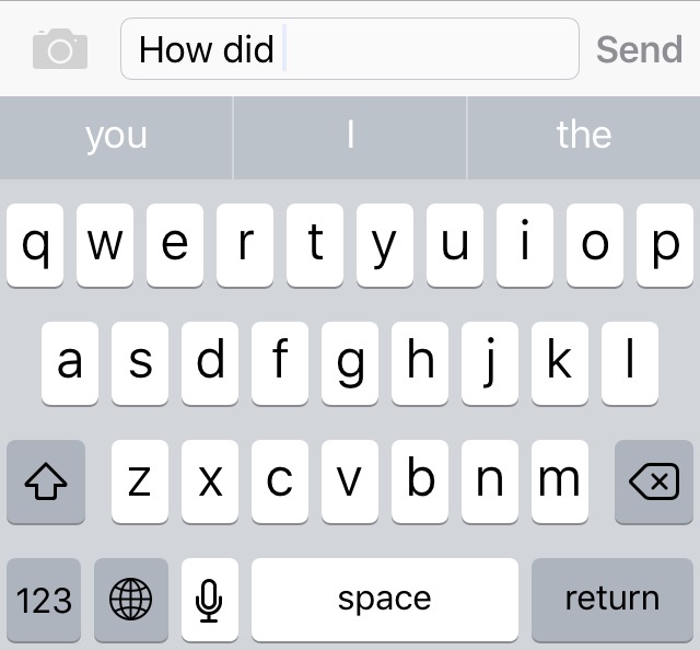
Figure 2.2: Predictive text input using language models. The underlying language model suggests the words you, I and the.

2.3 Applications

Because Brown clustering results both in a class-based language model and a hierarchical clustering, it has applications in two separate areas. The following subsections cover these.

2.3.1 Applications of Language models

Statistical language models can be used in applications such as:

• Predictive text input where a computer system can assist a human typing by suggesting the most likely words to be typed next. Figure 2.2 shows a smartphone keyboard assisting the user to type a text message. The figure shows a predictive input systems presenting the next most likely words. The user can select one of the suggested words in order to have it copied into the input field, avoiding spending time on typing.

• A speech recognition engine can use language models to improve the accuracy of its prediction. For example, in the phrase We need software to recognize speech, the section recognize speech sounds almost the same as wreck a nice beach. A speech recognition engine can use a language model to infer from the context of previous words that the speaker is talking about speech recognition rather than destroying beaches.

2.3.2 Applications of Brown clusters

Besides assigning words to word equivalence classes, Brown clustering can create a hierarchical structure of the clusters, if allowed to continue performing merges past the $C$ parameter. The hierarchical structure is a binary tree where the $|V|$ leaves are the words of vocabulary $V$. All other nodes in the tree represent clusters formed from merges of the $|V|$ words. If one labels branches going out of any node using 1s and 0s, each cluster obtains a unique binary string. The strings can be used in order to provide features for Natural Language Processing tasks such as Named Entity Recognition [24, 28, 33]. Named Entity Recognition is the task of identifying and classifying names of persons, organizations and places in a given text. Besides Named Entity Recognition, the tree resulting from Brown clustering can also be used to generate features for dependency parsing [17]. [21] continued on this path and expanded the use of Brown clusters to Chinese word segmentation.

2.4 Summary

This chapter presented statistical language models, an automatic modelling method for human language. Statistical language models use a representative corpus of text in order to estimate transitions between words in a language. However, these models tend to generalize poorly and are difficult to train due to the large number of parameters requiring estimation. Class-based language models address this by reducing the number of parameters requiring estimation. Class-based language models first assign words to classes, and then estimate probabilities of transitioning between classes using a corpus text. Finally, the chapter covered some of the applications of language models and of the hierarchical cluster structure resulting from Brown clustering.

Chapter 3 Related Work

This chapter presents a review of research in statistical language modeling (Section 3.1) and work on alternative methods for building statistical language models (Section 3.2.1). The review then moves on to the rather limited work on trying to improve class-based language models (Section 3.2.2) and in Section 3.3 it provides a short discussion of similar work on general agglomerative clustering, of which Brown clustering is an instance.

3.1 Statistical language models

Because of the variety of important applications, statistical language models have been heavily researched with different methods presented in the last few decades. Besides the $n$-gram models, of which class-based models are part, there is research considering alternative algorithms and methods for building statistical language models. Of these I mention models based on random forests, recurrent neural networks and methods using decision trees. All of these methods are covered by [29] in his survey that presents two decades of research on statistical language models. For a comparison of these various algorithms, I point the reader to a benchmark article by [8].

However, very little research has been done towards improving class-based language models. Some work has focused on smoothing language models [9], while some researchers such as Peter F. Brown have focused on industry application of machine translation and speech recognition as attested by a large number of patents filed. For a while it was believed that there is no need to improve the statistical language modeling techniques, but that focus should be put on collecting ever larger training corpora [5]. However, more recent research seems to disprove the idea and suggests moving focus back to improving the language models themselves [11]. In the following sections I will review the research on Brown clustering.

3.2 Class-based $n$-gram models

3.2.1 Basic algorithms

Brown, Desouza and Merger [7] introduced class-based language models in order to reduce the number of language model parameters that require estimation, in an effort to strike a trade-off between generalization power of language models and accuracy. [7] achieve the reduction by collapsing vocabulary words into word equivalence classes and then building a first order Markov Model using the word equivalence classes. In order to establish how words are mapped to word equivalence classes (word clusters) [7] perform a bottom-up, hard, hierarchical clustering of all words in the vocabulary. The original specification of Brown clustering, however, suffers from some ambiguity as discussed in Chapter 4. Despite this and because of the syntactic and semantic meaning of the word equivalence classes, Brown clustering became a common tool in Natural Language Processing, as described in Section 2.3.2.

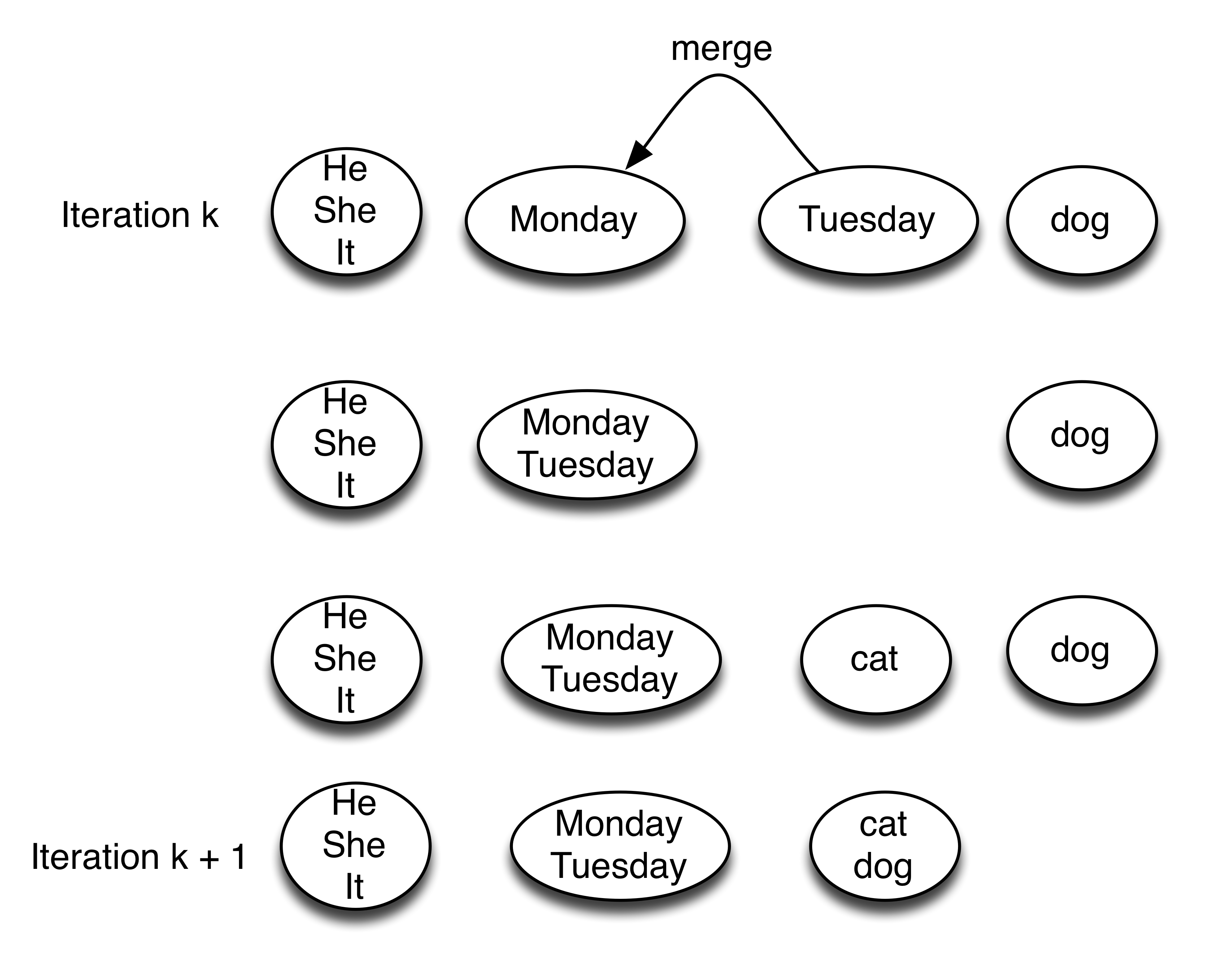
(a) The Brown Algorithm merges two clusters at every iteration step. At every iteration a new word is introduced into the computation window.

	FROM	TO
$w_{1}$	$c_{1}$	?
$w_{2}$	$c_{2}$	?
$w_{3}$	$c_{2}$	?
$w_{4}$	$c_{2}$	?
$w_{5}$	$c_{3}$	?

(b) In each iteration, the Exchange Algorithm must decide where to move each word of every cluster.

Figure 3.1: High-level view of Brown clustering and the Exchange Algorithm

The exchange algorithm was proposed by [26] as an alternative to Brown clustering. The exchange algorithm can be used in class-based language models to completely replace [7]’s clustering algorithm. It starts with an initial mapping (covered in section 3.2.2) from words to classes. It then considers for each element of every cluster, how the quality of clusters would improve if the specific element were to be part of every other cluster. The algorithm then performs those moves that lead to the highest increase in quality, resulting in a new clustering. Moving a word from one cluster to another is called an exchange, hence the algorithm’s name. One thing to note is that in each iteration of the exchange algorithm every word is reassigned to a cluster (which does not necessarily have to be a different cluster from its original one). The choice of moving each word depends only on the clustering at the beginning of the iteration and not on any of the move decisions already made during the iteration. The algorithm iterates either for a specified number of times or until a quality threshold is reached. The stopping criterion is a parameter to the algorithm.

The exchange algorithm is quite different from Brown clustering in several ways. Figure 3.1 shows a high-level comparison between the Brown algorithm and the Exchange algorithm. Firstly, the Exchange Algorithm allows for words to switch from the cluster they have first been assigned to, unlike Brown clustering. At every iteration, the Exchange Algorithm must decide for every word in the vocabulary, to which cluster it should be moved to. In contrast, the Brown clustering algorithm, at every iteration, performs a non-reversible merge of two clusters. The Exchange Algorithm always uses the entire vocabulary and set of clusters for every exchange decision. It has no faster, restricted version that provides an approximation, like the windowed variant of Brown clustering. Secondly, some domain knowledge can be included in the exchange algorithm (see section 3.2.2). Lastly, the Exchange Algorithm does not generate a hierarchy of clusters. Its output consists solely of the final clustering.

The exchange algorithm might seem similar to the k-means [22] clustering algorithm, which also iteratively creates clusterings over a collection of points. The k-means algorithm has the concept of cluster center and a distance from points to the center of a cluster. The exchange algorithm doesn’t have cluster centers. Its optimization goal, the average mutual information defined later on, in Equation 4.4, is a function over the interaction of all words, rather than a distance function. Brown clustering and the Exchange Algorithm have the same optimization goal.

[23] extended the class-based language models proposed by [7] by defining a version that uses tri-grams as the basis for class assignment, in effect constructing a class-based language model that uses a second order Markov Model where the probability of a word $w_{k}$ is

$$P(w_{k}|w_{1},w_{2},\dots w_{k-1})=P(w_{k}|c_{k})P(c_{k}|c_{k-1},c_{k-2})$$

where $c_{k-1}$ and $c_{k-2}$ are the clusters (word equivalence classes) for words $w_{k-1}$ and $w_{k-2}$ respectively. However, [23] do not follow the bottom-up clustering method proposed by [7] Instead, [23] use the exchange algorithm proposed by [26]. [23] classify their method as a top-down approach because it starts with the desired number of clusters and refines the clusters. However, no hierarchical structure is generated by their approach, distinguishing it from Brown clustering and limiting its applications to class-based language models only (see Section 2.3.2 for a short discussion on some applications of the hierarchical structure).

[23] start by assigning the first $C-1$ most popular words to individual clusters and the remaining words to cluster $C$. They then run the exchange algorithm for a user defined number of iterations, or until no more improvements are obtained. The optimization goal here is to increase the average mutual information value, similar to [7]’s algorithm. However, [23]’s algorithm maintains a set of $C$ clusters over the entire corpus at every iteration. Because of this, [23]’s algorithm can be considered an anytime algorithm. The Exchange Algorithm stops when it reaches a specified number of iterations or threshold of quality. Because of this it does not construct a hierarchy over the word clusters like Brown clustering does. The exchange algorithm makes local optimizations, and because of this, like [7]’s clustering algorithm, it does not guarantee an optimal clustering (i.e. the one that maximizes the amount of mutual information).

Another interesting aspect of the Exchange Algorithm is that it can allow for the input corpus to be modified. This aspect is not covered in the literature. Given clustering $C_{1}$ of a corpus $T_{1}$, one can provide the Exchange algorithm with clustering $C_{1}$ as initialization for clustering another corpus $T_{2}$. This technique could be used as a way to provide a good initialization for clustering a large corpus. It could also be used to improve the clustering of a vocabulary as more corpus data is collected. This rather obvious aspect of the Exchange Algorithm is not present in the Brown clustering algorithm where, given a higher quality (or longer) version of a corpus, one must start clustering from the beginning.

The problem of improving the quality of Brown clustering is a young research topic. So far efforts have focused on three main directions: good initialization, hyper-parameter tuning and improvements in word allocation to classes.

3.2.2 Improvement directions

Effect of initialization

[23] approach the question of improving quality of clustering from the view point of selecting a better initialization strategy. The algorithms proposed by [23] and by [7] both initialize by picking the first $C$ most often occurring words in the corpus. The original papers do not provide a motivation for ordering words by frequency. Section 4.2.1 tries to provide some arguments as to why frequency ordering makes sense and what some of its disadvantages are. In the Brown clustering algorithm, ordering by frequency leads to the clustering process being dominated by high frequency words as they establish what the first clusters are. [23] studied multiple ways of initializing the clustering algorithm such as random selection of words for initial classes, using the top most frequent words as well as an initialization strategy based on Part of Speech classes. In the Part of Speech experiment, words were assigned to one of the 33 classes defining parts of speech as found in a lexicon. The remaining classes were filled in with the most frequent words in the corpus. Their experiments showed no significant increase in average mutual information, leading them to conclude that either word class assignments are independent of initial word classes or a better method is still to be found. However, [23] only evaluate the average mutual information on a test corpus and do not evaluate on real word natural language processing tasks. The test corpus in [23]’s work is a shorter text that is completely separated from the corpus used to derive word clusterings. This follows the usual approach in Machine Learning, where data is separated into a large portion that is used for learning and a smaller one that is used exclusively to evaluate performance. The reasoning for such a split is to force the learning algorithm to optimize for the test set, without giving it the possibility to learn from the test set. In this way, the algorithm’s generalization is measured, rather than how well it fits the data in the learning set.

Hyper-parameter tuning

[32] investigated the effects of tuning the hyper-parameter $C$ (number of desired clusters) on the quality of Brown clustering by utilizing the resulting clusters in two classic natural language processing tasks: part of speech tagging and named entity recognition. [32] do not propose a new algorithm, but evaluate the effects of various values of $C$ (number of clusters) on clusters obtained with [7]’s original algorithm. They also scale the corpus size to see if, for fixed $C$, corpus size increases always produce better features.

Their experiments show an increase in cluster quality with an increase in corpus size. Similarly, an increase in the number of word classes leads to better clustering quality. However, they also show that performance tends to plateau and even decrease, when the number of clusters increases too much, or the corpus becomes too large, leading to noisy word classes. [32] conclude by recommending researchers try out various parameter values for Brown clustering. They also strongly advise against the common practice of setting the $C$ parameter to the fixed value of 1000.

Improvements in cluster quality

Another research direction for cluster quality improvement has been explored by [12]. In their work, [12] propose the hyper parameter $C$ (number of clusters) be separated from the window of data considered for cluster merging. In the original Brown algorithm, the $C$ parameter defines an implicit window within which the greedy algorithm selects from all pairs of clusters ($C^{2}$ in total) the best candidates for a merge. [12] remove this restriction by introducing a new parameter $a$ that defines the size of the active set to be used for considering cluster mergers. The separation of $C$ and $a$ allows for a large search space for cluster mergers (which can easily be dealt with by modern computers) without requiring an increase in the number of clusters ($C$) that often leads to lower quality clusters as mentioned above. [12] also developed a different method for generation of features from the tree structure resulting from Brown clustering by making more use of the average mutual information of the clustering. They applied it to Named Entity Recognition, but the method is not application specific.

3.3 Similar work in hierarchical clustering

Since the Brown clustering algorithm provides a hierarchical clustering of word classes, one should also consider work done on general hierarchical algorithms. Information theory has been applied to hierarchical clustering [1, 18, 31, 19]. However, these approaches generally rely on assumptions of Euclidean space providing some similarity measures that are used at various points during the clustering process.

In traditional hierarchical clustering, several approaches have been studied in order to improve the quality of clustering. [30] proposed a method to find the best trade-off between the number of clusters and quality according to an evaluation metric. The method makes use of a property of graphs, plotting the number of clusters versus quality: the sections before and after the ideal number of clusters are often approximatively linear. The L method proposed by [30] searches for the point in the graph that most exhibits this trait. That point will be selected as the ideal number of clusters.

For metric spaces [27] have proposed a hierarchical clustering algorithm with a theoretical cost of at most eight times that of the optimal k-clustering. The cost of a clustering is defined as the largest radius of its clusters. The algorithm uses the farthest-first traversal of a set of points in order to establish an order for points in the dataset. The farthest-first traversal of a set of points starts by randomly selecting a point. All subsequent points are selected so that they are furthest away from all the points that have already been selected:

$$\forall i>2,\ i=\operatorname*{arg\,max}_{i}\ \min{d(i,j):j\in\{1,2,\dots i\}}$$

[27] construct edges between the points in the farthest-first traversal by using the concept of granularity. At a granularity level of $l$, one can only see points $p$ from the dataset that are at least a distance $R_{l}$ from the first $l$ selected points. The distance $R_{l}$ becomes geometrically smaller as the granularity level increases. The graph is iteratively split into connected components. All points in a connected component are allocated to the same cluster. The iterative splitting process constructs the hierarchical clustering structure.

[4] proposed a hierarchical clustering algorithm that, given that the data to be clustered respects some properties, can work in an inductive way. More specifically, given a small subsample of the data to be clustered, the algorithm can create a hierarchical clustering structure that generalizes to the entire data set. For readers interested in more information on hierarchical clustering I would like to point the reader to a current survey of such algorithms by [25].

3.4 Summary

This chapter presented previous research on statistical language models (Section 3.1). Section 3.2.1 then covered the basic algorithms available for computing Brown clusters. A review of the rather limited work on quality improvements was presented in Section 3.2.2 followed by a review of related work on other hierarchical clustering algorithms in Section 3.3.

Chapter 4 Analysis of Brown clustering

This chapter provides an in depth description of the Brown clustering algorithm in Section 4.1. Following, Section 4.2 covers some novel insights into the importance and effects of underspecified parts of the Brown clustering algorithm.

4.1 Introduction and notation

In their work, [7] favour a less formal definition of the Brown clustering algorithm. For example, [7] does not provide a pseudocode description of the algorithm. In this section, I will try to present a more formal definition of the algorithm following the work of [12]. My hope is that providing a more formal definition of my changes will help in the effort of creating implementations of my proposals and in repeatability of my work. To my knowledge there are only two openly available implementations of the original Brown clustering algorithm: One written in C++ by [20][21] and one in python by [14]. In the following section I will refer to the two implementations when discussing details of the Brown clustering algorithm. Another thing I should mention is that most of the literature on Brown clustering uses the term token to denote any element that can be clustered. This means both words and punctuation marks (like “.”, “-” or “!”) are clustered. In the rest of this document I will use the term words to mean the exact same thing as the literature means with the term token. I made this choice in order to avoid burdening the reader with extra terminology.

Let the input $S$ be a corpus of text with a vocabulary $V$ of size $|V|$. By $V[k]$ I will denote the $k$’th word in vocabulary $V$. I will use the term word rather liberally to denote both actual language words like dog or the, but also punctuation signs like ? (question mark) or ( (open parenthesis). The definition of words used here is case sensitive, so the words The and the are distinct words in the vocabulary $V$. This is meant to capture the cases where capitalization indicates completely different concepts. For example no is the English negation while No is shorthand for number and Danish is an adjective referring to things originating in Denmark (such as this thesis) whereas danish is a delectable pastry. The common case where the capitalized and non-capitalized words denote the same concept is trivially handled by Brown clustering as the words will have a similar usage pattern (this will become clearer later in the chapter).

I will use $C$ for the parameter denoting the number of clusters, $C_{k}$ to denote a clustering which is a collection of $C$ disjoint clusters $C_{k}(1),\dots,C_{k}(C)$ containing one or more words from the vocabulary $V$ so that each word from $V$ is assigned to one cluster. The $k$ subscript identifies $C_{k}$ as being the clustering resulting after $k$ merge steps of the Brown clustering algorithm. Formally,

$$C_{k}(i)=C_{k}(j)\implies i=j,\ \ \forall i,\ j$$

$$|C_{k}(i)|\geq 1,\ \ \forall i,\ k$$

$$\bigcup_{i}C_{k}(i)=V,\ \ \forall k$$

$p(C_{k}(i),C_{k}(j))$ will be used to denote the probability that a word in class $C_{k}(i)$ follows a word in class $C_{k}(j)$. If we consider this over all the clusters available, we end up with a matrix of co-occurrences, which I will also refer to as the occurrence matrix. The occurrences will be derived from the input corpus $S$ by counting. For shorthand, I will use the notation $p(i,j)$ to index into the occurrence matrix at row $i$ and column $j$. By $pl(C_{k}(i))$ and $pr(C_{k}(i))$ we will denote the left and right probabilities of cluster $C_{k}(i)$. By probability left (respectively right) of $C_{k}(i)$ I mean the probability of any word in $C_{k}(i))$ appearing before (respectively after) any word $m$ in the vocabulary $V$ (including itself):

$$pl(i)=\sum_{m=0}^{|V|}p(i,V[m])$$ (4.1)

$$pr(i)=\sum_{m=0}^{|V|}p(V[m],i)$$ (4.2)

Since using $C_{k}(i)$ to denote the $i$’th cluster can become tedious, I will also refer to cluster $C_{k}(i)$ as simply $i$, where this doesn’t create any confusion. Therefore, $pl(C_{k}(i))$ is going to be the same as $pl(i)$.

The Mutual Information of two clusters $i$ and $j$ will be denoted by

$$MI(i,j)=p(i,j)\log_{2}\frac{p(i,j)}{pl(i)pr(j)}$$ (4.3)

The Average Mutual Information (AMI) of a clustering $C$ is the sum of the mutual information of any two clusters $i$ and $j$:

$$AMI=\sum_{i,j\in C_{k}}MI(i,j)$$ (4.4)

Even though it is an average, Equation 4.4 does not contain any divisions as each mutual information term is weighed through the use of $p(i,j)$ in Equation 4.3.

A merger of two clusters $C_{k}(i)$ with $C_{k}(j)$ with $i<j$ is the operation of moving all words from cluster $C_{k}(j)$ into cluster $C_{k}(i)$. I will use the short notation $i+j$ to denote the merger of cluster $C_{k}(i)$ with $C_{k}(j)$. Mergers of the form $i+i$ are not allowed. Given this notation, we have the following equations for all $i$, $j$, $m$, including $m=i+j$:

$$p(i+j,m)=p(i,m)+p(j,m)$$ (4.5)

$$p(m,i+j)=p(m,i)+p(m,j)$$ (4.6)

$$pl(i+j)=pl(i)+pl(j)$$ (4.7)

$$pr(i+j)=pr(i)+pr(j)$$ (4.8)

$$MI(i+j,m)=p(i+j,m)\log_{2}\frac{p(i+j,m)}{pl(i+j)pr(m)}$$ (4.9)

$$MI(m,i+j)=p(m,i+j)\log_{2}\frac{p(m,i+j)}{pl(m)pr(i+j)}$$ (4.10)

Equations 4.6 and 4.10 are not present in the original paper by [7], but they follow the implied idea of the algorithm. Being a greedy algorithm, Brown clustering will choose to merge those two clusters that lead to the lowest loss in average mutual information. [7] define the loss in average mutual information as

$$L(i,j)\equiv AMI-AMI(C_{k}\setminus C_{k}(i)\setminus C_{k}(j)\cup C_{k}(i+j)),$$ (4.11)

where the second term is the average mutual information of the clustering $C_{k}$ where clusters $i$ and $j$ have been merged. Although not specified in the original paper, a merge of two clusters doesn’t necessarily lead to a lower average mutual information. This is the reason for using the equivalence symbol ($\equiv$) in Equation 4.11. The simplest example is to consider what would happen in the windowed algorithm (presented later in this chapter), when we merge two words that have no occurrence with any cluster in the window, including each other. Their mutual information is 0 (since the nominator in Equation 4.3 is 0). Similarly, the mutual information terms will be 0 for every pair of clusters where one of them is one of the clusters being merged. So, the total loss in AMI loss is 0. In practice, the equivalence should be read as an equal sign since a minimization of the difference will lead to the clusters that have the lowest negative impact on the average mutual information.

The algorithm starts by considering each word in the vocabulary as being its own cluster. Given that we have $|V|$ words in the vocabulary, and we need $C$ clusters, there are $|V|-C$ merges that have to be performed. I only focus here on the merges necessary for going from $|V|$ words to $C$ clusters. This will not generate the hierarchical structure described in Chapter 2. In order to achieve that, a total of $|V|$ merges are necessary, $|V|-C$ in order to obtain $C$ clusters, and $C$ merges in order to complete the hierarchical structure. The class-based language models are already derived after the first $|V|-C$ mergers, which is why I only focus on these in this document. The complete hierarchy is only necessary for the Natural Language Processing applications described in Section 2.3.2, and, anyway, a straight-forward adaptation of the ideas presented here.

Returning to the first $|V|-C$ mergers, at each step we must consider a merge of any two pairs of possible clusters. In order to make any merge we need to consider $\frac{(|V|-k-1)^{2}}{2}$ combinations. We start with $|V|$ clusters (one for each word) and after $k$ iterations we have $|V|-k$ clusters left, since every iteration merges two clusters. There are $(|V|-k-1)^{2}$ pairs possible at every iteration since we don’t allow a cluster $w_{k}$ to be merged with itself. Performing the merge $i+j$ is the same as $j+i$. Because of this, we only need to check half of the pairs, hence $\frac{(|V|-k-1)^{2}}{2}$ combinations. However, checking all these possibilities might take a long time.

[7] proposed two approaches to address this. The first one is a dynamic programming approach to the clustering problem. Generally, a dynamic programming algorithm splits a problem into smaller subproblems. When solving each subproblem, the algorithm saves the result of the subproblem (along with other relevant data). When the algorithm runs with the same subproblem, or a superset of the subproblem, the cached data structure can be used to either immediately retrieve the correct result, or use it to quickly compute a result for the larger problem. Thus, a dynamic programming algorithm can provide faster computation at the expense of some memory usage. In the Brown clustering algorithm, the dynamic programming approach allows for the next pair of clusters to be merged and next AMI to be calculated from data at the current iteration, at the expense of caching some larger data structures in working memory (Random Access Memory), more specifically, the loss in AMI and the quantity of mutual information for every hypothetical merge under consideration.

I have chosen not to incorporate the dynamic programming version of Brown clustering as the focus of this thesis is not on performance, but on quality of results. Non-dynamic programming versions of the algorithm are easier to modify.

The second approach is a windowed algorithm. The windowed algorithm starts by creating one cluster per word, just like the initial Brown clustering algorithm. But, unlike the initial algorithm, the windowed version uses only a subsection of the $|V|$ initial clusters in order to make merge decisions. The window is set to $C+1$ and at each iteration one merge is performed inside the window, followed by the introduction into the window of a cluster from the ones left outside of the window. Thus, at every iteration there are $C+1$ clusters in the window. However, the algorithm’s focusing only on clusters in the window reduces its search space and thus its ability to find optimal solutions. When there are no more clusters to include in the window the algorithm proceeds like the initial Brown algorithm until only one cluster is left. In an attempt to alleviate the effects of the restricted search space, [12] proposed that the window be made into a parameter to the algorithm. This allows windowed Brown to use windows that are larger than $C$, thus making better merge decisions. A pseudocode representation of the windowed Brown clustering algorithm is presented in Algorithm 1. Lines 1 and 2 create the initial $C$ clusters out of the most frequent $C$ words. Lines 3 to 11 represent the main algorithm loop. On lines 4 - 5 the merge leading to the lowest loss is performed and the resulting cluster used to replace the cluster with the lower index in the merge. Then, lines 6 - 11 insert another word into the merge window if that is possible, otherwise they remove the extra cluster. Please note that Algorithm 1 does not describe the part of Brown clustering that generates the hierarchical structure as it is not a focus of this thesis.

Algorithm 1 The windowed Brown algorithm

0:  sequence S, number of clusters C

1:  for $i=0$ to $C+1$ do

2:        include word $i$ in window as $C_{i}$

3:  for $i=0$ to $|V_{S}|-C$ do

4:        $(C_{i},C_{j})\leftarrow best\_merge(C,\ C+1,\ C+1)$ {$best\_merge$ is defined in Algorithm 5 on page 5}

5:        $C_{i}\leftarrow C_{i\leftarrow j}$

6:        if $i+C+1\neq|V_{S}|$ then

7:              include word $V_{S}[i+C+1]$ as $C_{j}$

8:        else

9:              for $k=j$ to $C+1$ do

10:                    $C_{k}=C_{k+1}$

11:              remove cluster $C_{C}$

The two approaches described above, using dynamic programming and using a window, are theoretically complementary. It should be possible to use them together in order to speed up computations and reduce the algorithm run time. However, the mathematical equations covering the dynamic programming version (equation 17 in the paper by [7]) only cover the non-windowed Brown clustering algorithm. Furthermore, only a textual description is provided for the windowed version. Because of this situation, it is not directly possible to implement a version of Brown clustering taking advantage of both approaches. The biggest challenge in deriving equations to make the dynamic programming version compatible comes from the fact that newly inserted words can have a serious effect on the interaction of clusters in the window. Inserting a new word into the window will always increase the average mutual information as it adds $C$ new terms to the sum in Equation 4.4. These $C$ newly added terms affect the costs of making any merge.

4.2 Novel insights into windowed Brown clustering

The windowed algorithm assumes words in the vocabulary are sorted in descending order of their frequency. The first $C+1$ words are taken together and the two of them that result in the lowest loss in AMI are merged together. Then, the next most often occurring word is included into the window until and the process is repeated until all words have been assigned to one of the $C$ clusters. However, up to now, researchers have not considered how essential parts of the algorithm such as word order and breaking ties affect clustering quality.

4.2.1 Importance of ordering words

In the original algorithm, clusters are seeded by those words with highest frequency, and words are included into the window in order of their frequency (most frequent first). But, there is no argumentation for sorting words by their frequency. Presumably, the hope in selecting the most often occurring words (as opposed to the least frequent ones, for example) is that the occurrence matrix will be less sparse, more accurately reflecting the cost of merging clusters, leading to better merge choices. If the algorithm is to limit its search space by using a window, one would want to start by filling the said window with a good set of words. One would also like to include words into the window in an order that would help the restricted algorithm make good merge choices. Some work related to good initialization has been covered in Section 3.2.2. However, that work applies only to the exchange algorithm since Brown clustering does not start with an initial clustering of all words in the vocabulary.

As mentioned before, not all transitions between words (or word equivalence classes) is expected to appear in any training corpus. For many clusters $i$ and $j$, the joint probability is $p(i,j)=0$, which leads to a sparse occurrence matrix. Because $p(i,j)$ is the first term in the definition of mutual information (see Equation 4.3), for many cluster combinations, the mutual information will be zero. For clusters with a mutual information of zero, a merger will result either in no loss, or a very small loss. Such a merge is very tempting for the greedy Brown algorithm. This situation can be exacerbated by the order in which words are included in the merge window.

Let us consider what would happen if one were to include in the merge window a word that happens not to occur before or after any of the words already inside the merge window, but that occurs rather often before words that are not inside the merge window. Let us say the word we have inserted is dog and the words outside the window that dog appears together with quite often might be adjectives like bad, good or smelly. The newly included word (dog) will have a mutual information of zero with any word already in the window because it does not appear together with any of the words in the window. This leads to a zero loss in AMI for any merge, so dog will be merged with almost any cluster in the window, depending on the implementation of Brown clustering. We know, however, that dog has a positive value of mutual information with some words outside the window. When any of those words are brought into the window, say smelly, their mutual information value will be higher with the cluster that contains dog, because the word dog is a member of the cluster. In absence of any occurrences of words in the window with dog it was assigned to a pretty much random cluster. We find ourselves in the situation where a random cluster has a high mutual information with the newly inserted word (smelly), thus affecting the merge decision at the current step.

4.2.2 The window’s effect on probabilities

From the original paper it is not clear how the merge window should affect all of the probabilities defined in Equations 4.1 to 4.10 above. Should $pl$ and $pr$ only count occurrences within the window, or the entire corpus? If we use the global counting for $pl$ and $pr$, we will get values more representative of the actual use of words in the corpus. If we limit them to the window, we obtain values that are more representative of the interaction of words within the window. When using the values over the entire corpus $pl$ and $pr$ have almost the same value (there will be two words for which the values will differ by one, namely the first and last word in the corpus). Using the locally computed values is computationally more expensive. Using the locally computed values, we will also see much larger discrepancies between $pl$ and $pr$ and this can change the values of mutual information since both $pl$ and $pr$ are part of the mutual information formula (see Equation 4.3). In both my implementation and the one by [20], the original values for $pl$ and $pr$ are used, i.e. they are not limited to only occurrences with words in the window.

If we consider a run of windowed Brown over the corpus in Figure 4.1(a) with parameter $C=2$, the initial window will contain words . (period), the and cats. With a global count for $pl$ and $pr$, the word the will have values 5 and 4, respectively. With local counts, however, they become $pl=2$ and $pr=0$ as we only count bi-grams with words already in the research window. For $pl$, there are two instances of the bi-gram the cats and for $pr$, there are no bi-grams consisting of a word in the window, followed by the word the. Since $pr$ is 0, any pair consisting of the word the on the right side will have a mutual information of 0, while all pairs with the on the left side will have an increased value of mutual information as local $pl$ is less than half the value of global $pl$. The locally counted, lower valued, $pl$ and $pr$ will increase the cost of any merge involving the word the.

4.2.3 Handling words with the same rank

The algorithm does not specify how words with the same frequency should be arranged in the total ordering that dictates their inclusion into the window. This can have considerable implications over the merges that are performed, depending on how often the equal frequency words appear together with words already in the window.

Table 4.1: Word frequencies

rank	word	no. occurrences
1	.	5
1	the	5
2	cats	3
3	dog	2
3	likes	2
3	Alice	2
4	chased	1
4	scared	1
4	ran	1
4	away	1
4	sports	1

ΨΨthe dog chased the cats .
ΨΨthe dog scared the cats .
ΨΨthe cats ran away .
ΨΨAlice likes cats .
ΨΨAlice likes sports .
ΨΨ

(a)

ΨΨthe dog chased the cats .
ΨΨAlice likes cats .
ΨΨAlice likes sports .
ΨΨthe dog scared the cats .
ΨΨthe cats ran away .
ΨΨ

(b)

Figure 4.1: Two similar corpora with the same vocabulary, frequency count and co-occurrences

(a) Clustering with AMI = 1.1411

ΨΨ the likes
ΨΨ . Alice chased ran scared away
ΨΨ cats dog sports
ΨΨ 

(b) Clustering with AMI = 1.1373

ΨΨ the likes ran
ΨΨ . Alice chased scared
ΨΨ cats dog away sports
ΨΨ 

(c) Clustering with AMI = 1.1218

ΨΨ the Alice away
ΨΨ . chased ran scared
ΨΨ cats dog likes sports
ΨΨ 

Figure 4.2: Various clusterings that can result from using different interpretations of Brown clustering over the two corpora in Figure 4.1. Each row represents one cluster.

Consider the corpus in Figure 4.1(a) with word frequencies specified in Table 4.1. If we run the Brown clustering algorithm with parameter $C=3$, it starts by making a window of size $4$ and including the $4$ word with highest frequency. The first three of these are: . (period), the and cats. The fourth most often occurring word is difficult to establish. Is it dog, likes or Alice? They all have the same number of occurrences. Actually, [7] do not define what should happen in these situations. By leaving the behavior unspecified, we can arrive at different implementations providing different clusterings. By continuing the example in Figure 4.1(a), I will also show that the order in which the aforementioned words are included can have a significant effect on the value of average mutual information.

Let us consider what would happen if the corpus is changed from the one in Figure 4.1(a) to the one in Figure 4.1(b). Neither the values of $pl$, nor $pr$, will change since we have the same words in the vocabulary and they appear the same number of times. The occurrence matrix will also stay the same as the word . (period) will still appear two times before the word the and two times before the word Alice. The two corpora should have similar clusterings. Because of the unspecified behavior mentioned above, the order words are included in the merge window changes. This leads to different mergers and, subsequently, to different final clusterings and values of average mutual information.

In both my implementation, and that of [20], the clustering and final average mutual information for parameter $C=3$ changes if the corpus is changed between the ones in Figure 4.1. We will notice a change in average mutual information between 1.1411 and 1.1218 as my implementation switches from the clustering in Figure 4.2(a) to the one in Figure 4.2(b) and [20]’s changes from the clustering shown in Figure 4.2(c) to the one in Figure 4.2(b). At a first glance the change in average mutual information seems small, but we should remember that merges earlier in the clustering process can have a significant impact on merges later in the process. We can see that clustering in Figure 4.2(a) does not just have the highest average mutual information, but is also an assignment that follows more closely with the kind of clustering we, as humans, would expect given the meaning and syntactic role of words.

There is one final thing to note. The issue presented in this section applies not only to sorting words by frequency. It also applies to the case where words are sorted by connectivity (the amount of distinct words appearing after each word in the vocabulary), or any other sorting for that matter. Actually, this issue is not at all specific to Brown clustering and can affect any sort of windowed hierarchical clustering algorithm.

4.2.4 Handling non-unique minimal mergers

Another aspect of tie breaking not specified by [7] is how the clustering algorithm should handle cases where there are several pairs of clusters that, if merged lead to the same, equal minimum loss in average mutual information.

For this, another problem must be addressed first. When do we consider losses of average mutual information to be equal? Here, we have to take into account the fact that, very often, the difference between the lowest loss and the second lowest loss is smaller than 1. And, because the calculation of average mutual information involved lots of operations on floating point numbers, as clustering progresses, approximation errors become more pronounced.

One approach in breaking this tie could be to perform all merges that result in the lowest loss in average mutual information. However, this becomes problematic when the pairs of clusters to merge are not disjoint. Another approach could be to perform the second lowest loss in AMI and hope that the resulting clustering would break the tie.

4.3 Summary

In this chapter I presented an in-depth look at the Brown clustering algorithm. I described the three versions of the algorithm originally proposed by [7]: the non-windowed algorithm, the non-windowed algorithm using dynamic programming and a windowed version of Brown clustering. The second part of the chapter revealed a number of serious issues in the definition of all versions of the Brown clustering algorithm. They doesn’t take into account the effect of word ordering, words with same frequency or ties between different lowest loss mergers. Through the use of examples I made an argument for the considerable and undesired effect these omissions can have on the quality of resulting word clusters.

Chapter 5 Quality Improvements

In this chapter, I describe two algorithmic changes to Brown clustering. The first one, RESORT (Section 5.1), is meant to provide a more information theoretic method of sorting words in a corpus and to be a starting point for general discussions about the idea of using a dynamic word order. The second modification, ALLSAME (Section 5.2), aims at addressing some undefined algorithm behavior identified in Chapter 4 by guiding merge decisions.

5.1 Word ordering

Section 4.2.1 addressed the choice of [7] to sort words by frequency, before inserting them into the merge window. In this section, I propose a variation of the Brown clustering algorithm that does not maintain a static word order, but in which the order words are inserted into the merge window depends on the words that are already in the window.

Sorting words can be motivated by the desire to maximize the amount of information about words already in the window. Sorting words by frequency is one method that aims at achieving this goal. A simple alternative is to sort words by their connectivity. That is, for every word $w$, count the number of unique words in the vocabulary $V$ that appear before or after $w$ in a given corpus. Sorting by connectivity will tend to create a dense occurrence matrix in the merge window (low number of zeros), while sorting by frequency will tend to have a higher number of zeros, but larger values for the non-zero values.

I propose words be sorted by the amount of mutual information they have with words already in the merge window. This can be measured by computing the sum of mutual information between every word not in the merge window and every cluster in the merge window (see Equation 4.3 for the formula of mutual information). The resorting can be made after every merge or, in order to reduce the computational cost, after every $R$ merges.

To give an intuition of the algorithm, let us consider the corpus in Figure 5.1, with word frequencies presented in Table 5.1, and a run of the resorting algorithm where the desired number of clusters $C$, is set to 3. The initial merge window will have a size of $C+1=4$ and contain the words: Margrethe, to, the and II. After the first merge, the word . (period) will be inserted into the merge window, and the remaining words will be resorted. I will now focus only on the 5 words of rank 3. By computing the amount of mutual information between these words and clusters in the merge window, RESORT can derive a new ranking. We do not need to compute the values of mutual information to understand the example. We only need to count the number of co-occurrences with words already in the merge window. By looking at Figure 5.1, we can see that words in, her and heir have no co-occurrences with any of the 5 words already in the window and thus have a mutual information of 0. The word throne has one co-occurrence (the throne) and the word Majesty has two (both of the form Majesty Margrethe). Because of the higher number of co-occurrences, the word Majesty has more mutual information with clusters in the merge window and thus, becomes the next word to be included into the merge window. In this case, re-sorting words outside the window has managed to break the tie between words with the same frequency. By first inserting the word Majesty, the algorithm has also chosen to involve for merge considerations the word it knows most about, relative to the clusters already in the window. I ignored all other words in this analysis because they either have a mutual information value of 0 (because of no co-occurrences), or a small one (because of having only one co-occurrence).

ΨΨMargrethe II was born on the April 16 1940 .
ΨΨMargrethe II succeeded to the throne in 1972 ,
ΨΨbecoming Her Majesty Margrethe II.
ΨΨHer Majesty Margrethe II only became heir presumptive in 1953
ΨΨwhen changes to the constitution allowed Margrethe to be a
ΨΨlegal heir to the throne.
ΨΨ

Figure 5.1: A corpus that can benefit from re-sorting words not already in the merge window.

Table 5.1: Word frequencies for the corpus in Figure 5.1

rank	word	no. occurrences
1	Margrethe	4
1	to	4
1	the	4
1	II	4
2	.	3
3	throne	2
3	Majesty	2
3	in	2
3	her	2
3	heir	2
4	all other words	1

Algorithm 2 The RESORT algorithm

0:  sequence S, number of clusters C, interval for resorting R

1:  for $i=0$ to $C+1$ do

2:        include word $i$ in window as $C_{i}$

3:  for $i=0$ to $|V_{S}|-C$ do

4:        $(C_{i},C_{j})\leftarrow best\_merge(C,\ C+1,\ C+1)$ {$best\_merge$ is defined in Algorithm 5 on page 5}

5:        $C_{i}\leftarrow C_{i\leftarrow j}$

6:        if $i+C+1\neq|V_{S}|$ then

7:              include word $V_{S}[i+C+1]$ as $C_{j}$

8:        else

9:              for $k=j$ to $C+1$ do

10:                    $C_{k}=C_{k+1}$

11:              remove cluster $C_{C}$

12:        if $i>0$ and $i\ \bmod\ R=0$ and $i\neq|V_{S}|-C$ then

13:              $resort\_words(C,V_{S},V_{S}[i+C+2]$

In Algorithm 2, listing the RESORT approach, the desired number of clusters is denoted by $C$, while $C_{index}$ is used to denote a specific cluster in the current clustering. Lines 1 and 2 insert the first $C+1$ words into the merge window. The algorithm then performs the best merge of two clusters (lines 4–5) and inserts the next cluster (lines 6–7). On line 5, cluster $C_{i}$ is replaced by $C_{i\leftarrow j}$, the cluster resulting from the merger of clusters $C_{i}$ and $C_{j}$. If there are no more clusters left to insert, the algorithm is at the end of its run, so it removes the last $C+1$’th cluster in order to obtain the $C$ clusters required (lines 9–11). Lines 12–13 resort all words starting with the next word to be inserted into the window. A general approach to resorting is presented in the pseudocode. Resorting can be done after each merge, or after every $R$ merges. The $R$ parameter allows the user to trade off a better word sorting for a shorter run time, if the resorting process is computationally slow. The cost of resorting the next words to include depends on the chosen sorting function.

The $resort\_words$ function takes as input the current clustering, an ordering of words $V_{S}$ and a pointer $i$ to one of the words in this ordering. It then resorts all words between $i$ and $|V_{S}|$. The resorting criteria can be any function that can provide a total ordering. I propose that words be ordered by the amount of mutual information they have with words already in the merge window. I chose the amount of mutual information with words in the merge window as a resorting criteria because it involves both connectivity and number of occurrences together with words already in the merge window. Connectivity is measures the number of unique words that appear in a bi-gram with any given word. Frequency measures how often a given word appear in a corpus, as shown in the third column of Table 5.1.

5.2 Handling words with same ranking value

As discussed in Chapter 4, the Brown clustering algorithm does not specify a strategy for dealing with words that have the same number of occurrences in the corpus. As I have shown in Section 4.2.3 of Chapter 4, word order is an important algorithmic consideration that can affect the final clustering. This raises some deeper questions about repeatability of scientific work of researchers using Brown clustering as input in their work, or as a pre-processing step. For some examples of work using Brown clustering as input or for pre-processing, see [12, 17, 21, 24, 33]. With the current state of things (word order determined ambiguously), different implementations of Brown clustering will provide different final clusterings with unpredictable fluctuations in quality. In the most widely used implementation of Brown clustering, the one by [20], the order of words with the same number of occurrences is defined by the implementation of sorting in the Standard Library of C++. However, if using different compilers or different implementations of the Standard Library of C++, even [20]’s implementation could provide different clusterings and values of average mutual information, just by changing the compilation environment.

The inclusion order of words with same number of occurrences must be taken into account and a behavior specified. A first idea could be to include as many of the words sharing the same number of occurrences as possible into the merge window. We could use the ideas in the Generalized Brown clustering proposed by [12] in order to separate the window from the $C$ parameter. To remind the reader, [12] proposed that the window size be separated from the $C$ parameter so that users must specify how large the window size should be (though a minimum of $C+1$). The idea is that a larger window size should allow the clustering algorithm to make better local decisions given that it has more options to choose from. We could then run the original algorithm using $C+1$ clusters and, at every inclusion of a word into the merge window, we would check if the next word has the same number of occurrences in the corpus. If yes, we would also include the next word and continue including either until we encounter a word that has a different number of occurrences, or we reach the $w$, the window size. That is, we try to take all words with the same number of occurrences in at once.

However, there are a few issues with this approach. Because we might reach the window size limit before we run out of words with the same number of occurrences, we must decide which words to include into the window. A simple solution is to increase the window size $w$ so that the limit can never be reached. In other words, if we set $w=|V|$, the window will always be able to contain all words with the same number of occurrences. Including many words at a time reveals another problem. As the clustering progresses, the algorithm encounters more words with the same number of occurrences (see the flattening line in Figure 5.2).

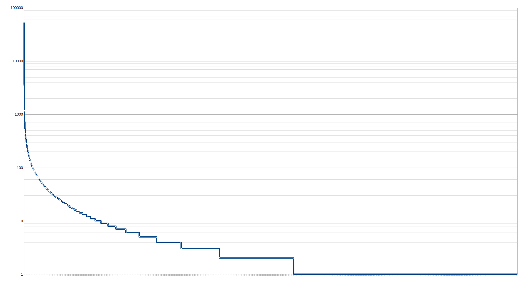
Figure 5.2: Frequencies of the most frequent 100 words in a corpus of length $1\,000\,000$ and vocabulary of size $56\,000$. A wider step means more words with the same frequency.

When the algorithm reaches words with a small number of occurrences, it encounters more words sharing the same number of occurrences and might have to include hundreds, or maybe thousands, of words into the merge window. At this point in time, the greedy merge strategy will behave quite unexpectedly. Because of the algorithm’s greedy nature, it will always choose to merge those clusters that lead to the smallest loss in average mutual information. When thousands of words with a small number of occurrences are included in the merge window, the algorithm will have a tendency to pick one-word-clusters and merge them together, since they will generally have a merge cost very close to zero. In time, as the window shrinks to approach the size $C$, the one-word-clusters will be merged into two-word-clusters and so on, as they become larger clusters. As the window size $w$ approaches $C$, the loss in average mutual information will increase exponentially since the algorithm will have to merge together larger and larger clusters.

The behavior described above is not present in the original windowed Brown clustering because the merge window only receives one word at a time. Almost exclusively, the last cluster inserted into the window (which is a single-word-cluster) is merged into an already existing cluster. This generally happens at a low cost to the average mutual information.

We have seen that including only one word at a time poses the problem of choosing an order over words with the same number of occurrences. We have also seen that the straight-forward solution of including all words with the same number of occurrences can lead to a smaller average mutual information. I propose we do not include any word at all, in the method I call ALLSAME.

When encountering several words with the same number of occurrences the algorithm should temporarily enlarge its merge window so as to include all these words and then temporarily change its merge strategy. It should no longer allow mergers between any two clusters, but enforce the requirement that at least one of the merged clusters was part of the merge window before the last mass inclusion (a citizen cluster). This way, the greedy merge strategy is prevented from lumping together single-word-clusters into larger clusters that it then deals with expensively. The requirement also deals with the problem of choosing between words with the same number of occurrences, since all candidates are brought into the window. Figure 5.3 illustrates the conceptual split of the clusters in the merge window.

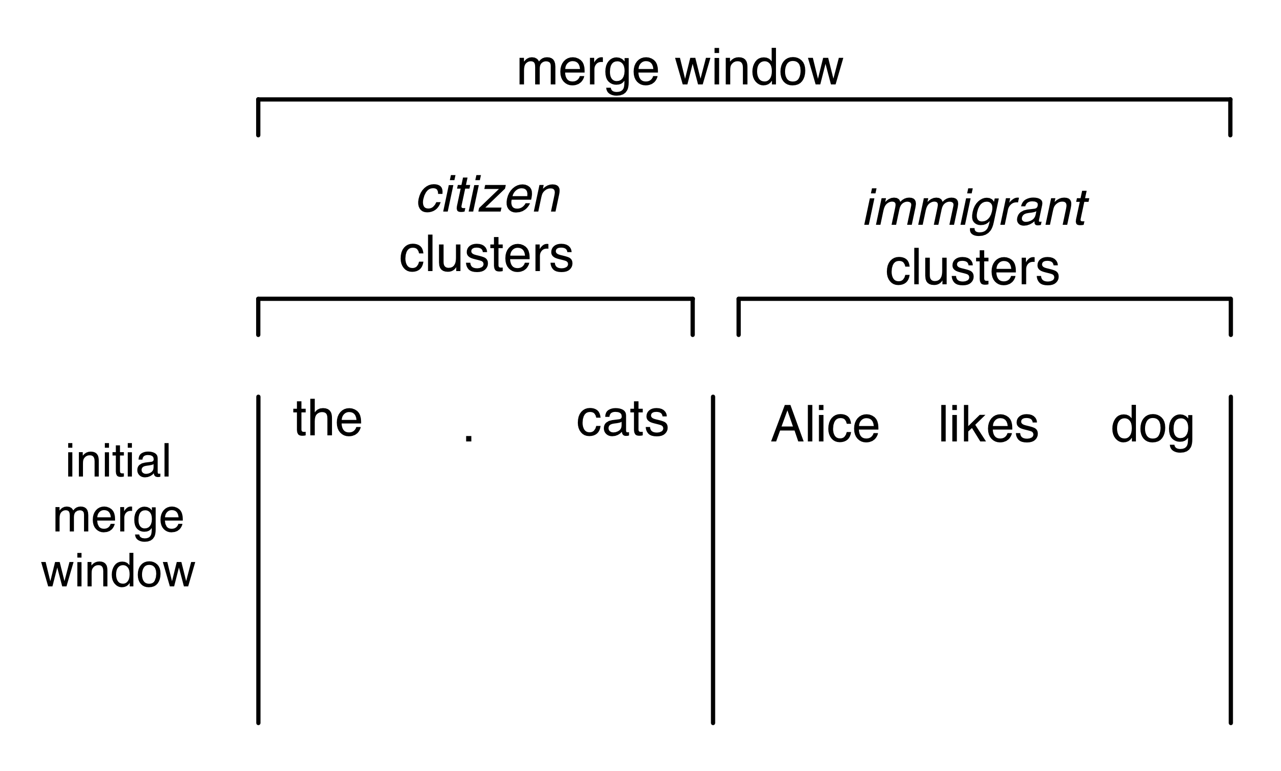
Figure 5.3: The conceptual split of the merge window in the ALLSAME algorithm. Any merger must contain at least one cluster from the left section. The figure represents the initial merge window state when starting the ALLSAME algorithm on the corpus from Figure 4.1.

After a mass inclusion, the algorithm will continue making merges, but no inclusions. As time passes, and the merge window will become smaller and there will be fewer candidates from the original window. When the merge window reaches size $C$, it will consist of two types of clusters: larger versions of those that were present in the merge window before the mass inclusion, and a group of single-word-clusters that were included as part of the mass inclusion. The single-word-clusters are those whose merger presented the highest loss in average mutual information. The single-word-clusters can now become “citizens“ of the merge window, meaning that at the next mass inclusion they will be allowed to participate in mergers with new immigrants. Algorithm 3 presents the pseudocode of the algorithm described above.

Algorithm 3 The ALLSAME algorithm

0:  S, C

1:  $merge\_limit,\ current\_window\_size=initial\_inclusion(S,\ C)$ {$initial\_inclusion$ is defined in Algorithm 4 on page 4}

2:  for $i=0$ to $|V_{S}|-C$ do

3:        $(C_{i},C_{j})\leftarrow best\_merge(C,\ merge\_limit,\ current\_window\_size)$ {$best\_merge$ is defined in Algorithm 5 on page 5}

4:        $C_{i}\leftarrow C_{i\leftarrow j}$

5:        for $k=j$ to $current\_window\_size-1$ do

6:              $C_{k}=C_{k+1}$

7:        if $current\_window\_size=C$ then

8:              $merge\_limit\leftarrow C$

9:              if $i+current\_window\_size\neq|V_{S}|$ then

10:                    $k\leftarrow i+current\_window\_size$

11:                    $occurrences\_previous=occurrences[k]$

12:                    while $occurrences[k]=occurrences\_previous$ do

13:                          include word $V_{S}[k]$ as $C_{k}$

14:                          $k=k+1$

15:                          $current\_window\_size=current\_window\_size+1$

16:        else

17:              $current\_window\_size\leftarrow current\_window\_size-1$

18:              if $i<C+1$ and $j<C+1$ then

19:                    $merge\_limit\leftarrow merge\_limit-1$

Line 1 of Algorithm 3 calls the initial_inclusion function described in Algorithm 4. initial_inclusion creates the initial clusters and merge window. This is done taking into account all words that have the same number of occurrences. If the words on position $C+1$ and $C+2$ have the same number of occurrences, both are included in the initial merge window as well as all other words that have the same number of occurrences. The $merge\_limit$ variable keeps track of the largest identifier of a cluster that can be allowed on the left side of a merge. Initially, this is set to be the identifier of the last word in the window that has the second largest number of occurrences (line 7 in Algorithm 4).

Algorithm 4 The $initial\_inclusion$ method

0:  S, C

1:  $merge\_limit\leftarrow 0$

2:  $previous\_occurrence\leftarrow 0$

3:  $i\leftarrow 0$

4:  loop

5:        if $occurrences[i]\neq previous\_occurrence$ then

6:              if $i\leq C+1$ then

7:                    $merge\_limit\leftarrow i$

8:                    $previous\_occurrence\leftarrow occurrences[i]$

9:              else if $i>C+1$ then

10:                    break

11:        include word $i$ in window as $C_{i}$

12:        $i\leftarrow i+1$

13:  return  $merge\_limit$, $i$

Lines 2 to 19 of Algorithm 3 contain the merge loop. In line 3 the best merge candidates are established by calling the function $best\_merge$ defined in Algorithm 5. This function iterates over all combinations of $i$ and $j$ that meet the requirement that $i<merge\_limit$ and return the best candidates. In line 4 the cluster $C_{i}$ is replaced by $C_{i\leftarrow j}$ which is the cluster resulting from the merger of $C_{i}$ and $C_{j}$. In lines 5 and 6 the empty hole left after the merger of $C_{j}$ is covered by moving all clusters $C_{k}$ with $k>j$ one position to the left. This strategy for covering empty holes is different from the ones used so far. [12] consider the collection of current clusters to be a set, so removals are easy. [7] propose moving the last cluster in the clustering into position $j$. In ALLSAME , the order of clusters is important as it is used when deciding which clusters can be part of merges.

When the merge window reaches size $C+1$ the $merge\_limit$ variable is reset to the value $C$ (line 8). Lines 9 to 15 take care of including all words that share the next highest number of occurrences. Lines 17 to 19 update the merge window size and $merge\_limit$ after a merge that is not followed by an inclusion.

When run with $C=3$ and $w=11$, ALLSAME will return the clustering in Figure 4.1(b) when given either the corpus in Figure 4.1(a) or the one in Figure 4.1(b). A clustering independent of the order words appear in the corpus is what we want as this way, results are reproducible. In Figure 5.4 I show a step by step diagram of ALLSAME’s merge decisions. One can see both at the initial merge window and the merge window after iteration 3, that ALLSAME makes its merge decisions based on all words with the same frequency, not just on words that appear first in the corpus (like the windowed Brown clustering does).

Algorithm 5 The $best\_merge$ method

0:  C, $merge\_limit$, $current\_window\_size$

1:  for $i=0$ to $merge\_limit$ do

2:        for $j=i+1$ to $current\_window\_size$ do

3:              calculate loss of merging $C_{i}$ with $C_{j}$

4:  find $C_{i}$ and $C_{j}$ with smallest loss

5:  return  $C_{i}$, $C_{j}$

Figure 5.4: A step by step run of the ALLSAME algorithm on the corpora from Figure 4.1. The algorithm is run with parameters $C=3$ and $w=8$.

5.3 Summary

In this chapter I presented RESORT and ALLSAME, two modifications to the Brown clustering algorithm meant to address the issues described in Chapter 4. The RESORT algorithm re-sorts words not in the merge window after every $R$ merges. This allows it to make informed inclusion (and subsequently merge) decisions based on the amount of average mutual information. I have shown through examples how RESORT is better making inclusion decisions than the windowed Brown algorithm. The second part of the chapter presented ALLSAME, a modification that solves the issue of words with the same frequency. ALLSAME temporarily includes all words with the same frequency into the merge window and then imposes some restrictions on which clusters can be part of mergers. By taking into account all clusters with the same frequency, ALLSAME makes better merge decisions and is expected to outperform windowed Brown in the amount of final average mutual information.

Chapter 6 Empirical validation of both clustering and the resultant language models

In the previous chapter, I proposed two changes to the windowed Brown clustering algorithm: ALLSAME (Algorithm 3) expands the merge window to include all words with the same frequency and imposes some restrictions on which clusters can participate in mergers. RESORT (Algorithm 2) uses a dynamic sorting of the vocabulary in order to create merge windows with the largest possible amount of average mutual information.

In this chapter I present an experimental evaluation of the two changes. I measure cluster quality though average mutual information. In order to obtain some idea of real world effects of the various algorithm changes, I also measure performance of the class-based language models that result from the word clusterings.

I start by describing the data sets used in experiments (Section 6.1). I then provide an overview of the various metrics employed and the choice for said metrics (Section 6.2). Then, I describe reproducibility details of the implementation (Section 6.3). The last section in this chapter contains all experiment results and analyses (Section 6.4).

6.1 Data set selection and retrieval

To construct the datasets, I started with a complete dump of all English Wikipedia articles as of September 1st, 2015 [13]. The choice of downloading all articles from Wikipedia was motivated by the fact that other widely available corpora are not good representations of language use. Corpora based on content from social networks, such as Twitter, contain too many abbreviations and inconsistent spellings. On the other hand, widely known corpora such those consisting of content from news agencies, have consistent spellings, but have a restricted use of language, guided by corporate style guides for journalists.

Before using the Wikipedia data, I first processed the data dump in order to remove most of the Wikipedia-specific markup using the wikiextractor script created by [2]. I then wrote a Python script to remove the remaining XML and HTML tags by finding all words that started and ended with angled brackets, and removing them. Finally, I generated 4 corpora of different lengths and vocabularies by taking 4 subsamples at of the Wikipedia corpus. Each of the 4 corpora starts at a different, random, location in the Wikipedia corpus and has no any overlap with the others. Corpora $T10$, $T20$, and $T50$ were used for clustering. The fourth corpus, $TT$, was used to evaluate the performance of class based models resulting from the various clustering algorithms. The corpora are named using the scheme $T[number\ or\ T]$ where digits indicate how long the corpus is, in thousands of words. The second $T$ in $TT$ stands for test. I decided to use corpora of smaller length and vocabulary after starting experiments on larger corpora and evaluating the estimated run time to completion. For example, the longest running algorithm would have required approximatively 300 days to complete on a corpus of length $1\,000\,000$ words with a vocabulary of approximatively $56\,000$ words. Finally, the SimpleTokenizer class from the Apache OpenNLP library was used to separate all words in every corpus.

I chose to generate a separate testing corpus in order to follow the common practice in Machine Learning of testing on samples that have not been used for learning. This is supposed to provide a better picture of how well models generalize to yet unseen data and avoid over-training. An overview of the data sets is provided in Table 6.1.

Name	Text Length	Vocabulary Size
T10	$10\,000$	2657
T20	$20\,000$	4420
T50	$50\,000$	8616
TT	$10\,000$	2815

Table 6.1: Overview of the corpora used in experiments.

[23] changed the vocabulary of their corpora by replacing low frequency words with a placeholder word. [7] also reduced the vocabulary size in their work, but they do not mention the method used to reduce vocabulary size. In order to experiment on real-world corpora, I made no changes to the vocabularies of my corpora. Generally, vocabularies are reduced in order to get rid of words with small frequencies, say, 1, or 2. Besides substantially reducing the vocabulary size, this normally creates a more dense co-occurrence matrix. On average, this increases the amount of information about every word in the remaining vocabulary. There are also some disadvantages to reducing the vocabulary size. For one thing, dropping words with low frequency severely reduces the vocabulary, which leads to reduced language models. Secondly, the common approach for reducing vocabularies is to replace undesired words with a placeholder word. Replacing lots of words with a placeholder word effectively clusters all those words into a massive cluster of unrelated words with no information theoretic basis and no particular reason for semantic nor syntatic similarity. The new cluster will have both high frequency and high connectivity with other words in the vocabulary, which might influence mergers in both the Brown clustering algorithm, as well as in the Exchange Algorithm.

6.2 Evaluation metrics

I evaluate my algorithms by measuring quality of clusters and performance of the resulting class-based language models. I measure the quality of clusters using Average Mutual Information (AMI), as defined in Equation 4.3 on page 4.3. Since higher AMI is the optimization goal of Brown clustering, the final value of AMI will show how well each algorithm has fulfilled its optimization goal. Even though only the final value of average mutual information matters in evaluating the quality of a clustering, I also measure the amount of average mutual information at every iteration of the clustering algorithm. This provides a clearer picture of how the various algorithms behave.

In order to evaluate cluster quality as part of language models, I used the models in conjunction with the testing corpus, $TT$. I measured perplexity for comparability with related work and class prediction accuracy in order to avoid some weaknesses of perplexity.

Perplexity is a measure of both a model and the sample under test. It measures how well a model predicts the given sample. It is commonly used to measure performance of statistical language models (c.f., [6, 16, 15, 7, 23]). For bi-gram models like the one used in this thesis, perplexity is defined as [16]:

$$PP(W)=\sqrt[N]{\prod_{i=1}^{N}\frac{1}{p(w_{i}|w_{i-1})}}$$ (6.1)

where $N$ is the length of the test corpus. As its name implies, perplexity measures the amount of surprise a given test sample represents for a

$$CPA=\frac{\text{\# correctly predicted classes}}{\text{\# class predictions}}$$ (6.2)

specific model. If the model predicts a sample perfectly (i.e. for all $w_{i},\ w_{i-1}$, $p(w_{i}|w_{i-1})=1$), the value under the order $N$ root will be equal to $N$, resulting in a perplexity of 1. However, if the model does not predict the sample perfectly, the perplexity value increases. So, higher perplexity means a model is worse at predicting a given corpus. When I measure perplexity in my experiments, I do not take the order $N$ root, as the computation is both impractical and unnecessary. Since all language models trained on the same corpus have the same vocabulary, relative to a the testing corpus $TT$, they have the same number of transitions $N$, so their perplexity values are directly comparable even without the order $N$ root. Note that differences between language models are thus exponentiated by the missing root.

Even though perplexity has been used as an evaluation metric in previous research (c.f. [7, 23]), it is not a good performance measure for class-based models. This is because a class-based language model with $C$ classes can only predict $C$ words of the total words in a vocabulary. Class-based language models always predict the most popular word in each class. Equation 2.4 defined the probability of words in a class-based language model. When used for prediction, all language models return only the most likely word (i.e. the one with the highest probability). Given the form of Equation 2.4, this means a single word per class, effectively reducing the prediction vocabulary to one of size $C$ (number of clusters). In other words, for any word $w_{i-1}$ from class $C_{i-1}$, a class-based language model will always predict the same word $w_{i}$ from class $C_{i}$, where $w_{i}$ is the most often occurring word in class $C_{i}$. Because perplexity takes into account the probability of predicting every word in the vocabulary (including those that will not actually be predicted), it will always be overly positive about the performance of a class-based language model. There is no problem in using perplexity to evaluate non-class-based language models as they can predict all words in their vocabulary. However, I anticipate performance of all algorithms studied in this thesis to be weak in terms of perplexity.

In my experiments I report the perplexity of every language model, in order to keep in line with the currently used methods. However, I also include another performance metric, the Class Prediction Accuracy (henceforth CPA). This measures how often the language models predicts the class containing the next word. Since class-based language models can be used for reducing the search space for regular language models by limiting the candidate words to only those in a class, this metric is more appropriate than perplexity.

6.3 Implementation details

In order to evaluate my algorithms, I started by implementing the original Brown clustering algorithm. I knew from the beginning that Brown clustering is a slow algorithm. For that reason, I chose to implement everything in the C++ programming language in order to avoid the slowdowns that come with using high level virtual machines such as those for the Java and Python programming languages.

I found out that a lot of development time is wasted if, on every run of Brown clustering, the computer must read the corpus, reorder words, and then construct the necessary data structures. In order to avoid this wasted time I created data structures common to all my variations and implemented separate steps for this operation. My implementations can read a corpus into the data structure and persist the data structure to a file. This is done by making use of the Boost Serialization library.They can take a data structure from a file and reorder words, and, of course, can read a data structure from a file and perform Brown clustering. A similar approach is used for language models, which use a common data structure that is saved to a file at the end of clustering. Testing the language models is a separate step.

In order to reduce running time I tried, to the best of my ability, to parallelize work so as to take advantage of multiprocessor systems. I used OpenMP to parallelize work at various locations in each implementation. For example, most data structure initializations are performed in parallel, using static scheduling of threads. Computing every hypothetical merge and establishing the lowest loss is performed in parallel, using dynamic scheduling in order to account for the unbalanced amount of work.

In order to speed up the insertions of words into the merge window I constructed a data structure to keep track of which words appear together in the corpus. This allows for quicker insertions of low frequency words. Similarly, the code testing language models uses cached data structures to avoid expensive searches.

Finally I used separate machines for running learning tasks and running evaluation tasks. All experiments were performed on a workstation with two Intel Xeon E5-2687W v3 [10] and 128 GB of RAM. I ran all language model tests on a machine with an Intel Xeon E5-2650 and 32 GB of RAM. The choice of using two machines is motivated by the large run time necessary for experiments relative to the amount of time available for a masters’ thesis. Over the course of this thesis, between the various experiments, I have accumulated over 500 hours of computation time with a CPU utilization of over 80% across all twenty cores.

6.4 Results

In this section I report and discuss experimental results. First (Section 6.4.1), I look at how different windowing strategies affect the quality of clusters and performance of resulting class-based language models. Second (Section 6.4.2), I look at how the windowed version of Brown clustering (referred to as BROWN) performs as compared to the first algorithm proposed by [7], the non-windowed Brown clustering (referred to from now on, as BROWN_NW), implemented without the dynamic programming.

I illustrate the performance of language models and the final AMI by using tables. The plots show AMI values as clustering progresses. These help better understand why and how algorithmic decisions affect the final value of average mutual information by showing instantaneous change in mutual information and the quality of each micro-decision the algorithm makes.

In the following plots, I use short names to identify the various combinations of algorithms, parameters and corpora. In Table 6.1, I gave an overview of the short names for corpora. I use the following convention for naming experiment runs: [algorithm_name].[value of C parameter]. Where algorithm_name is one of BROWN (see [12] for a nice pseudocode expression of the algorithm), ALLSAME(Algorithm 3), RESORT (Algorithm 2) or BROWN_NW. The first three are described in Chapters 4 and 5. By BROWN_NW, I mean the version of Brown clustering that does not use any window but, instead, makes decisions over the entire vocabulary. This is the first algorithm proposed by [7].

Astute readers will notice that, in Figures 6.1, 6.2, 6.3, 6.4, 6.5 showing progressions of average mutual information, runs where the $C$ parameter is set to $200$ have a shorter line. This is the expected behavior of all algorithms. Since there are $|V|-C$ merges to be performed, runs where the $C$ parameter is set to a higher value will perform fewer merges. The reader should focus on the general shape of the plots and on the $y$-coordinate of the rightmost point in each line, rather than where on the $x$-axis the line ends. Lines corresponding to runs with higher values of $C$ are expected to always be higher than those corresponding to lower values of $C$. This is because the Brown clustering algorithm is not forced to make as many expensive choices when it can assign words to more clusters.

Figure 6.1: The average mutual information as the clustering algorithms progress on the T10 corpus.

Figure 6.2: The average mutual information as the clustering algorithms progress on the T20 corpus.

6.4.1 Evaluating the performance of clusters and language models generated with alternative windowing strategies

This section presents the quality differences between clusters generated by the original Brown clustering algorithm (denoted as BROWN) and the two algorithmic modifications proposed in Chapter 5: ALLSAME(Algorithm 3) and RESORT (Algorithm 2). ALLSAME and RESORT use a different windowing strategy from the windowed Brown algorithm. ALLSAME includes all words with the same rank into the merge window and imposes some restrictions on which clusters can participate in mergers. RESORT includes one word at a time into the merge window (like BROWN); however, it does not maintain a static ordering of words in the vocabulary. After every $k$ mergers, words not already included in the merge window are resorted by the amount of mutual information they have with words already in the window.

Clustering quality

Figures 6.1, 6.2 and 6.3 show a similar pattern over the three corpora, so I will discuss them together. The three plots show the amount of mutual information ($y$-axis) plotted against the number of mergers completed ($x$-axis). Each of the plots corresponds to one of the 3 learning corpora described at the beginning of this chapter. Each line represents the instantaneous amount of average mutual information. Only the final AMI is relevant in judging the quality of clusters. However, the progressions provide insights into the quality of each algorithm’s decisions. In these plots, good performance is synonymous with an upwards trending line with a high end point. It is expected that the amount of average mutual information increases, as more words are included into the window. Every new word in the window adds $2C$ terms to the summation for AMI (see Equation 4.3). A low frequency word increases AMI less. Because of the word’s lower frequency, there are more clusters for which the numerator in Equation 4.3 is zero (no co-occurrences), leading to more zero-valued terms in the summation. Every merger reduces the amount of AMI as it removes $2C$ terms from the summation in Equation 4.3 and because it increases the denominators in Equation 4.3.

The ALLSAME algorithm has a very specific pattern to its line, which does not occur with the other algorithms. ALLSAME’s average mutual information line displays a saw shape due to mass inclusions of words into the merge window. Every tooth in the saw corresponds to including all words with a specific frequency. The teeth vary in size because there are more words with a smaller frequency so, even though each word brings little mutual information into the merge window, the cumulative effect is larger. ALLSAME gains average mutual information over BROWN after each saw tooth.

ALLSAME ends by outperforming BROWN in 5 of the 6 runs, and it matches BROWN in the remaining (see last column in Table 6.2 for the actual values). This is due to the fact that every time ALLSAME encounters multiple words with the same frequency, it chooses its own order for merging these words based on their average mutual information with all words in the merge window. BROWN, on the other hand includes and merges same frequency words based on an undetermined order that is influenced by the order words appear in the original corpus (see the discussion in Section 4.2.3). Actually because ALLSAME makes better merge decisions than BROWN every time there are multiple words with the same frequency, ALLSAME should be expected to perform better than BROWN the more words with a given frequency there are (the larger the saw teeth), and the more often this occurs (the more teeth there are).

The RESORT algorithm is a little more subtle. Its average mutual information tends to be just slightly better than BROWN while the algorithms runs. However, final average mutual information of RESORT tends to be very close to that of BROWN (again, see last column in Table 6.2 for the actual values). This, however, should not be considered a null result. Experiments on much larger vocabularies and with different sorting strategies are necessary in order to determine whether RESORT is actually not better than BROWN. And, of course, performance of the resulting class-based language models should also be taken into account.

Performance of class-based language models

Having looked at the AMI progression of the algorithms, I now turn to the performance of the class-based language models that are generated from these clusters. Studying Table 6.2 in more detail, one notices quickly that clusterings with the highest value of average mutual information are not always the best performing ones (boldface). Actually, there is no clear winning language model either when measured by class prediction accuracy, or by perplexity. Nor is there any clear connection between vocabulary size and performance of the language models.

In 4 of the 6 setups, clusterings with the highest average mutual information are not the best performing ones, when measured by class prediction accuracy. Similarly, in 5 of the 6 setups, clusters with the highest average mutual information do not score best in perplexity. Furthermore, class prediction accuracy often (4 out of 6 times) disagrees with perplexity on which language models perform best. Another interesting aspect is that ALLSAME constantly achieves higher values of average mutual information, but this rarely translates into the best performance when evaluating the class-based language models.

Actually, the overall best language model according to class prediction accuracy is the one generated by RESORT on $T50$ with a $C=300$. This fact, together with the observations about ALLSAME lead to deeper questions. Why is it that higher AMI rarely translates into better class prediction accuracy or perplexity? Could it be that average mutual information is not an optimal metric to use as an optimisation goal in Brown clustering? The results indicate that more thorough investigation of AMI is necessary.

Figure 6.3: The average mutual information as the clustering algorithms progress on the T50 corpus.

Corpus	Language model	CPA (%)	PerplexityN	Final AMI
T10	ALLSAME.200	16.65	$1\,392\,340$	$\mathbf{3.88}$
T10	BROWN.200	$\mathbf{17.15}$	$684\,689$	3.69
T10	RESORT.200	16.58	$\mathbf{664\,733}$	3.70
T10	ALLSAME.300	15.99	$782\,654$	$\mathbf{4.33}$
T10	BROWN.300	17.06	$516\,494$	4.14
T10	RESORT.300	$\mathbf{17.38}$	$\mathbf{503\,967}$	4.15
T20	ALLSAME.200	$\mathbf{17.07}$	$6\,340\,400$	$\mathbf{3.26}$
T20	BROWN.200	15.89	$3\,993\,800$	3.17
T20	RESORT.200	15.46	$\mathbf{3\,686\,350}$	3.17
T20	ALLSAME.300	16.66	$3\,359\,050$	$\mathbf{3.69}$
T20	BROWN.300	$\mathbf{16.85}$	$2\,057\,020$	3.60
T20	RESORT.300	16.62	$\mathbf{1\,897\,490}$	3.59
T50	ALLSAME.200	15.73	$45\,033\,000$	$\mathbf{2.73}$
T50	BROWN.200	$\mathbf{16.56}$	$\mathbf{23\,851\,800}$	$\mathbf{2.73}$
T50	RESORT.200	16.50	$27\,125\,700$	$\mathbf{2.73}$
T50	ALLSAME.300	16.35	$25\,898\,900$	$\mathbf{3.17}$
T50	BROWN.300	16.52	$\mathbf{16\,686\,700}$	3.10
T50	RESORT.300	$\mathbf{17.30}$	$17\,850\,400$	3.10

Table 6.2: A qualitative overview of the various algorithmic changes proposed in this thesis. The best results in every metric shown in boldface. Quality is measured both directly on clusters through final average mutual information (the 5th column) and on the resulting class-based language models. The test corpus $TT$ is used to measure language model characteristics such as class prediction accuracy (3rd column) and perplexity (4th column).

6.4.2 Evaluating the idea of using a window

[7] proposed Brown clustering initially without the use of a merge window. The non-windowed Brown clustering algorithm starts by assuming every word is a cluster of its own and then iteratively performs $|V|-C$ mergers in order to obtain $C$ clusters. There are no inclusions in this algorithm since all words are part of the merge window from the beginning. This algorithm is denoted in the following figures by BROWN_NW. The windowed version (in my experiments denoted by BROWN) was proposed by [7] in the same paper as an approximation algorithm that can be run faster than the non-windowed Brown clustering algorithm. The windowed Brown clustering algorithm starts by assuming that the first $C+1$ most frequent words are clusters of their own. It then iteratively performs a merge of two clusters and then includes the next most frequent word into the merge window as a cluster. When there are no more words to include into the merge window, one more merge is performed in order to obtain $C$ clusters.

Figure 6.4: BROWN_NW versus BROWN on the T10 corpus.

Figure 6.5: BROWN_NW versus BROWN on the T20 corpus.

In Section 5.2, I made an argument against allowing mergers between any two clusters immediately after a mass inclusion. The argument was that when lots of low frequency, single-word clusters are introduced into the window, the greedy clustering strategy does not perform very well. However, if this is correct, it means that the non-windowed Brown clustering algorithm (BROWN_NW) should be perform worse than its approximation, the windowed Brown clustering algorithm. Actually, BROWN_NW should incur exponential increases in lost average mutual information. If we consider carefully the non-windowed version of the Brown clustering algorithm (which I refer to as BROWN_NW in all plots and tables), we realize that the algorithm starts by making a mass inclusion of all words in the vocabulary $V$. After this mass inclusion the algorithm performs $|V|-C$ mergers in order to obtain the $C$ clusters. In the following section I will present results of experiments comparing cluster quality between the original, non-windowed Brown clustering algorithm (referred to as BROWN_NW and the restricted, windowed, version (to which I will refer as BROWN). The windowed Brown clustering algorithm is the same algorithm as the brown-cluster (sometimes referred to as wcluster) implementation by [20], which is used ubiquitously in Natural Language Processing research.

Figures 6.4 and 6.5 follow the same design as Figures 6.1, 6.2, 6.3 and show the progression of average mutual information of BROWN against that of BROWN_NW. As expected, BROWN_NW incurs what seems like exponential loss in mutual information as it makes more mergers. This is obviously not the desired behavior for BROWN_NW. Actually the difference in average mutual information between BROWN and BROWN_NW seems to increase as the corpus size increases. In order to confirm this, experiments on larger corpora should be executed. Unfortunately, I cannot show the results of BROWN against BROWN_NW on the $T50$ corpus as the large computational complexity of these experiments prevented them from being finished before the deadline for this thesis.

Table 6.3 shows the language model performance metric and average mutual information of BROWN_NW. For easier comparison I have included the performance numbers for BROWN from Table 6.2. As suggested earlier in this subsection, BROWN achieves a higher average mutual information than BROWN_NW. This happens on both corpora. However, the situation is quite mixed when it comes to performance of language models. In 3 of the 4 setups, BROWN achieves better class prediction accuracy than BROWN_NW. The situation is different when considering the values for perplexity. Similar to Table 6.2, good average mutual information or class prediction accuracy are not necessarily indicators of good perplexity.

Corpus	Language model	CPA (%)	PerplexityN	Final AMI
T10	BROWN.200	17.15	$684\,689$	3.69
T10	BROWN_NW.200	17.06	$901\,309$	3.62
T10	BROWN.300	17.06	$516\,494$	4.14
T10	BROWN_NW.300	16.81	$486\,449$	4.11
T20	BROWN.200	15.89	$3\,993\,800$	3.17
T20	BROWN_NW.200	17.36	$3\,890\,810$	3.03
T20	BROWN.300	16.85	$2\,057\,020$	3.60
T20	BROWN_NW.300	16.64	$1\,745\,120$	3.51

Table 6.3: A qualitative comparison between using a window (BROWN) and not having a window, equivalent to running clustering over the entire corpus (BROWN_NW). Quality is measured both directly on clusters through final average mutual information (the 5th column) and on the resulting class-based language models. The test corpus $TT$ is used to measure language model characteristics such as class prediction accuracy (3rd column) and perplexity (4th column). Results for the $T50$ corpus are omitted as the experiments on such a large corpus take too long to complete.

6.4.3 Summary

In this chapter I showed and discussed results of running experiments to measure and compare the performance of my proposed algorithmic changes ALLSAME and RESORT. I also discussed results of experiments trying to confirm the counter-intuitive idea that the non-windowed Brown clustering algorithm (BROWN_NW) performs worse than the windowed version of Brown clustering (BROWN).

While I could show that ALLSAME can achieve better average mutual information than windowed Brown (BROWN), that result did not translate into better performance of the corresponding class-based language models. And while RESORT did not manage to achieve better values of average mutual information than BROWN, it did achieve better language model performance in some of the experiments. This behavior of RESORT suggests that the idea of dynamic word ordering should not be dismissed, but that different sorting criteria need to be investigated.

I managed to show that BROWN_NW achieves lower average mutual information than windowed Brown; however, that did not always translate into lower performance of the associated class-based language models. The lack of strong correlations, in both sets of experiments, between the performance of class-based language models and average mutual information raises some questions about the effectiveness of average mutual information as an optimization goal for Brown clustering.

Chapter 7 Conclusion and Future Work

7.1 Conclusion

Brown clustering is a hierarchical hard clustering algorithm designed to allocate words to clusters based on their usage in a learning corpus. Brown clustering has applications in the creation of class-based language models and for providing features for Natural Language Processing tasks.

Even though twenty-three years have passed since Brown clustering was proposed, not much research has been done towards improving the quality of resulting clusters, in spite of the fact that one of the two publicly available implementations has seen wide use in the research community.

In this thesis I have performed a close analysis of the Brown clustering algorithm to reveal some weaknesses. I have also provided two heuristics that address some of the shortcomings present in the original algorithm. I introduced ALLSAME, a modification of the windowed Brown clustering algorithm to solve the question of which of the words with same frequency should be included first into the merge window. ALLSAME  includes all words with the same frequency into the merge window, but enforces some restrictions as to which clusters are allowed to participate in mergers. My second proposal, RESORT, challenges the idea of a static word order. RESORT reorders words not already included in the window after every $k$ merges using the amount of mutual information with words already in the window as a differentiating dimension.

My experiments have shown that ALLSAME does consistently achieve better values of average mutual information. However, they have also shown that higher values of AMI are not strong indicators for high performing language models. Actually, the overall best performing language model was created by RESORT, which did not generally achieve the best AMI.

7.2 Future work

One of the major difficulties in running experiments for this thesis has been the long running times of Brown clustering which have prevented me from experimenting over larger data sets. My implementation makes use of CPU parallelism in order to speed up computations. Radically different implementations of the algorithm should be researched in order to make better use of parallelism capabilities already present in wide-spread CPUs and GPUs (graphics processing units). Another direction to follow is finding ways to distribute the algorithm so that is can be run on multiple computers at the same time. Similar research has been done on distributing the exchange algorithm [34], but not on Brown clustering.

I would also like to do some follow-up research on understanding the interplay between average mutual information and clustering quality. As my experiments have shown, higher values of average mutual information do not always lead to better language models. However, my experiments have not explored whether this is also the case for other uses of Brown clusters, such as the Natural Language Processing Tasks mentioned in Section 2.3.2. Actually, to my knowledge, there is no research on whether Brown clusters that perform well as classes for class-based language models are also good clusters for Natural Language Processing. Evaluation of cluster quality is a topic of interest in clustering research as clustering has generally proven difficult to evaluate.

Another research avenue I would like to pursue is incorporating external knowledge into the clustering algorithm. In his survey, [29] makes an argument for linguistic information being incorporated into statistical language models. Indeed, [23] tried to use parts of speech in order to initialize the Exchange Algorithm (see Section 3.2.2). I believe it might be interesting to explore the idea of assisting Brown clustering not just with linguistic information, but also with domain knowledge, or maybe even information from other clusterings.

Bibliography

- [1] M Aghagolzadeh, H Soltanian-Zadeh, B Araabi and A Aghagolzadeh “A Hierarchical Clustering Based on Mutual Information Maximization” In Image Processing, 2007. ICIP 2007. IEEE International Conference on 1, 2007, pp. I –277–I –280 DOI: 10.1109/ICIP.2007.4378945
- [2] Giuseppe Attardi “wikiextractor” [Online; accessed 24-October-2015], https://github.com/attardi/wikiextractor, 2015
- [3] Lalit R Bahl, Frederick Jelinek and Robert L Mercer “A maximum likelihood approach to continuous speech recognition” In IEEE Transactions on Pattern Analysis and Machine Intelligence IEEE, 1983, pp. 179–190
- [4] Maria-Florina Balcan, Yingyu Liang and Pramod Gupta “Robust Hierarchical Clustering” In Journal of Machine Learning Research. 15.1 JMLR.org, 2014, pp. 3831–3871
- [5] Michele Banko and Eric Brill “Scaling to Very Very Large Corpora for Natural Language Disambiguation” In ACL ’01 Proceedings of the 39th Annual Meeting on Association for Computational Linguistics Association for Computational Linguistics, 2001, pp. 26–33 DOI: 10.3115/1073012.1073017
- [6] Peter F Brown et al. “An Estimate of an Upper Bound for the Entropy of English” In Computational Linguistics 18.1 MIT Press, 1992, pp. 31–40
- [7] Peter F Brown et al. “Class-based n-gram models of natural language” In Computational linguistics 18.4 MIT Press, 1992, pp. 467–479
- [8] Ciprian Chelba et al. “One Billion Word Benchmark for Measuring Progress in Statistical Language Modeling”, 2014
- [9] Stanley F Chen and Joshua Goodman “An Empirical Study of Smoothing Techniques for Language Modeling” In Proceedings of the 34th Annual Meeting on Association for Computational Linguistics Association for Computational Linguistics, 1996, pp. 310–318 DOI: 10.3115/981863.981904
- [10] Intel Corporation “Intel® Xeon® Processor E5-2687W v3 (25M Cache, 3.10 GHz)” [Online; accessed 4-December-2015], http://ark.intel.com/products/81909/Intel-Xeon-Processor-E5-2687W-v3-25M-Cache-3_10-GHz
- [11] James R Curran and Miles Osborne “A very very large corpus doesn’t always yield reliable estimates” In Proceedings of the 6th conference on Natural language learning 20, 2002, pp. 1–6 Association for Computational Linguistics
- [12] Leon Derczynski and Sean Chester “Generalized Brown Clustering and Roll-up Feature Generation” To appear In Proceedings of the Thirtieth AAAI Conference on Artificial Intelligence, 2016
- [13] Wikimedia Foundation “English Wikipedia article content, September 1st 2015” [Online; accessed 24-October-2015], http://dumps.wikimedia.org/enwiki/20150901/enwiki-20150901-pages-articles.xml.bz2, 2015
- [14] Michael Heilman “tan-clustering” [Online; accessed 11-November-2015], https://github.com/mheilman/tan-clustering, 2013
- [15] Michele Jardino and Gilles Adda “Automatic determination of a stochastic bi-gram class language model” In Grammatical Inference and Applications Springer, 1994, pp. 57–65
- [16] F Jelinek, R L Mercer, L R Bahl and J K Baker “Perplexity — a measure of the difficulty of speech recognition tasks” In The Journal of the Acoustical Society of America 62.S1, 1977
- [17] Terry Koo, Xavier Carreras Pérez, Michael Collins and Others “Simple semi-supervised dependency parsing”, 2008
- [18] Alexander Kraskov and Peter Grassberger “MIC: Mutual Information based hierarchical Clustering” In Information theory and statistical learning, 2008, pp. 22
- [19] Alexander Kraskov, Harald Stögbauer, Ralph G. Andrzejak and Peter Grassberger “Hierarchical Clustering Based on Mutual Information”, 2003, pp. 11
- [20] Percy Liang “brown-cluster” [Online; accessed 28-October-2015], https://github.com/percyliang/brown-cluster, 2012
- [21] Percy Liang “Semi-supervised learning for natural language”, 2005
- [22] James MacQueen “Some methods for classification and analysis of multivariate observations” In Proceedings of the fifth Berkeley symposium on mathematical statistics and probability 1.14, 1967, pp. 281–297
- [23] Sven Martin, Jörg Liermann and Hermann Ney “Algorithms for bigram and trigram word clustering” In Speech Communication 24.1, 1998, pp. 19–37 DOI: 10.1016/S0167-6393(97)00062-9
- [24] Scott Miller, Jethran Guinness and Alex Zamanian “Name Tagging with Word Clusters and Discriminative Training.” In Proceedings of the North American Chapter of the Association for Computational Linguistics – Human Language Technologies 4, 2004, pp. 337–342
- [25] Daniel Müllner “Modern hierarchical, agglomerative clustering algorithms” In arXiv preprint arXiv:1109.2378, 2011
- [26] Hermann Ney, Ute Essen and Reinhard Kneser “On structuring probabilistic dependences in stochastic language modelling” In Computer Speech & Language 8.1 Elsevier, 1994, pp. 1–38
- [27] “Performance guarantees for hierarchical clustering” In Journal of Computer and System Sciences 70.4, 2005, pp. 555–569 DOI: 10.1016/j.jcss.2004.10.006
- [28] Lev Ratinov and Dan Roth “Design Challenges and Misconceptions in Named Entity Recognition” In Proceedings of the Thirteenth Conference on Computational Natural Language Learning Association for Computational Linguistics, 2009, pp. 147–155
- [29] Ronald Rosenfeld “Two decades of statistical language modeling: where do we go from here?” In Proceedings of the IEEE, 2000, pp. 1270–1278
- [30] S. Salvador and P. Chan “Determining the number of clusters / segments in hierarchical clustering/segmentation algorithms” In 16th IEEE International Conference on Tools with Artificial Intelligence IEEE Comput. Soc, 2004, pp. 576–584 DOI: 10.1109/ICTAI.2004.50
- [31] Noam Slonim, Gurinder Singh Atwal, Gašper Tkačik and William Bialek “Information-based clustering” In Proceedings of the National Academy of Sciences of the United States of America 102.51 National Acad Sciences, 2005, pp. 18297–18302
- [32] “Tune Your Brown Clustering, Please” In Proceedings of the conference on Recent Advances in Natural Lang Processing (RANLP), 2015, pp. 110–117
- [33] Joseph Turian, Lev Ratinov and Yoshua Bengio “Word representations: a simple and general method for semi-supervised learning” Association for Computational Linguistics, 2010, pp. 384–394
- [34] Jakob Uszkoreit and Thorsten Brants “Distributed Word Clustering for Large Scale Class-Based Language Modeling in Machine Translation” In Proceedings of the Association for Computational Linguistics, 2008, pp. 755–762