A Reverberation-Based Black Hole Mass for MCG-06-30-15

Abstract

We present the results of a reverberation campaign targeting MGC-06-30-15. Spectrophotometric monitoring and broad-band photometric monitoring over the course of 4 months in the spring of 2012 allowed a determination of a time delay in the broad H$\beta$ emission line of $\tau=5.3\pm 1.8$ days in the rest frame of the AGN. Combined with the width of the variable portion of the emission line, we determine a black hole mass of $M_{\rm BH}=(1.6\pm 0.4)\times 10^{6}$ M_⊙. Both the H$\beta$ time delay and the black hole mass are in good agreement with expectations from the $R_{\rm BLR}$–$L$ and $M_{\rm BH}-\sigma_{\star}$ relationships for other reverberation-mapped AGNs. The H$\beta$ time delay is also in good agreement with the relationship between H$\beta$ and broad-band near-IR delays, in which the effective BLR size is $\sim 4-5$ times smaller than the inner edge of the dust torus. Additionally, the reverberation-based mass is in good agreement with estimates from the X-ray power spectral density break scaling relationship, and with constraints based on stellar kinematics derived from integral field spectroscopy of the inner $\sim 0.5$ kpc of the galaxy.

1. Introduction

It has been a century since Edward Fath (1913) first observed strong emission lines originating in the nucleus of NGC 1068 and discovered the first active galactic nucleus (AGN). Yet it is only in the last 30 years that AGNs have become synonymous with supermassive black holes (e.g., Rees 1984) and that supermassive black holes have become synonymous with galaxy nuclei (e.g., Magorrian et al. 1998; Ferrarese & Merritt 2000; Gebhardt et al. 2000; Ferrarese & Ford 2005). Multiple independent lines of study focusing on a zoo of seemingly unrelated characteristics across the entire spectral energy distribution are now unified through our current understanding of the AGN phenomenon (e.g., Antonucci 1993; Urry & Padovani 1995). The mass and the spin of the black hole, its only quantifiable characteristics, are two key parameters in our understanding of not only AGN physics (e.g., Krawczynski & Treister 2013; Netzer 2015), but also galaxy evolution (e.g., Fabian 2012; Kormendy & Ho 2013; Heckman & Best 2014; King & Pounds 2015).

Astrophysical black holes can be characterized by their mass and spin, and being able to constrain both properties is rare. MCG-06-30-15 is one of only a handful of X-ray bright AGNs where its Fe K$\alpha$ emission may be studied in detail, allowing a measure of the black hole spin. Tanaka et al. (1995) first detected a broad red wing of the Fe K$\alpha$ emission line, as is expected due to the strong gravitational redshift and relativistic Doppler effects from material in the innermost accretion disk. Relativistic reflection models fit to the X-ray spectrum, including the Fe K$\alpha$ line, all indicate that the black hole spin is high, with a dimensionless spin parameter $a\gtrsim 0.9$ (Brenneman & Reynolds, 2006; Chiang & Fabian, 2011; Marinucci et al., 2014).

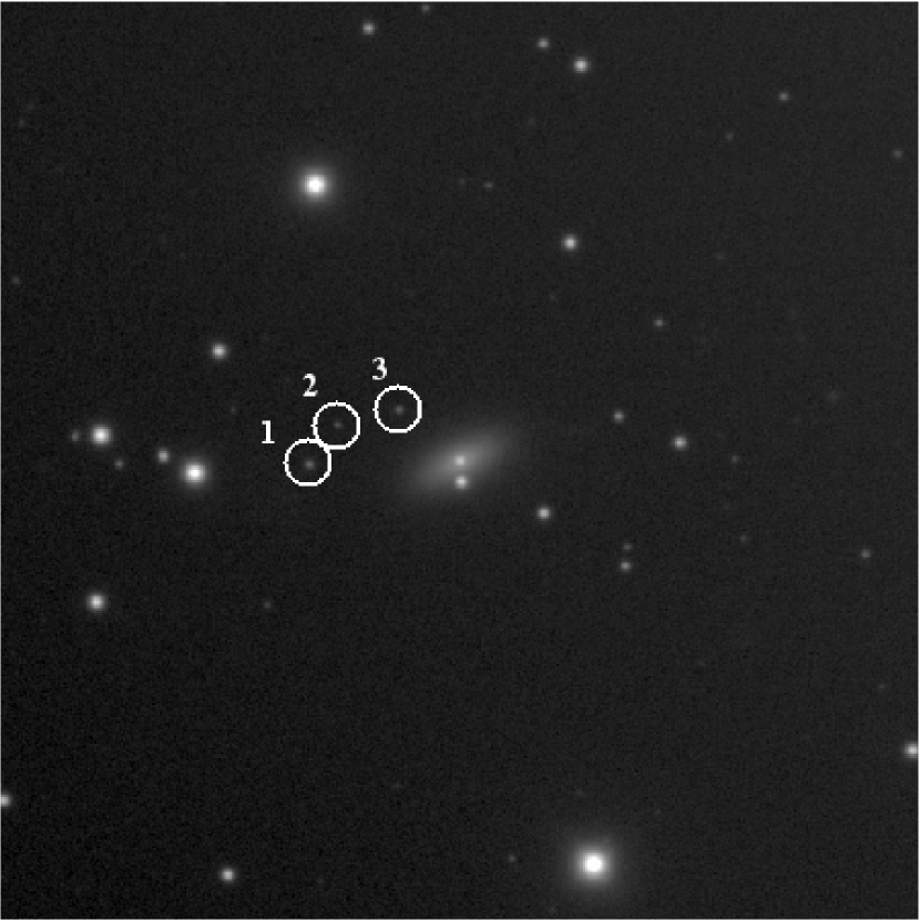
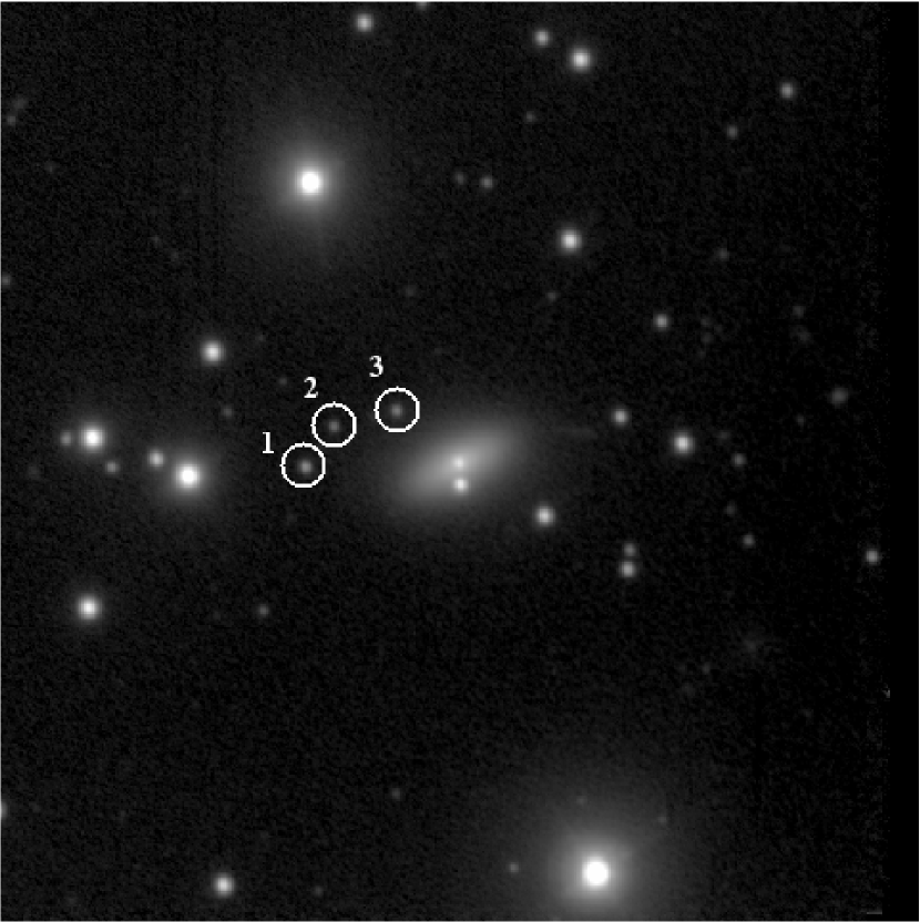
Figure 1.— Reference images for the $V-$band FTS dataset (left) and the $V-$band LT dataset (right). The region displayed is 4′$\times$4′, with north up and east to the left. The average exposure time for the FTS images is 20 s at a typical airmass of 1.3, compared to 60 s exposures for the LT images with typical airmasses of 2.3. The marked field stars are common to the ground-based images and the high-resolution HST image and were used to determine the absolute flux scale of the FTS and LT images.

While the spin has been constrained for a decade now, the black hole mass of MCG-06-30-15 is less well known. Previous estimates of the mass have relied upon scaling relationships such as the X-ray power spectral density break ($M_{\rm BH}=2.9^{+1.8}_{-1.6}\times 10^{6}$ M_⊙; McHardy et al. 2005) or the $M_{\rm BH}-\sigma_{\star}$ relationship ($M_{\rm BH}=3-6\times 10^{6}$ M_⊙; McHardy et al. 2005). High spatial resolution integral field spectroscopy of the inner $\sim 0.5$ kpc of the galaxy allowed Raimundo et al. (2013) to determine an upper limit on the black hole mass of $<6\times 10^{7}$ M_⊙, but the integration time was somewhat shallow and precluded a stronger mass constraint.

Reverberation mapping (Blandford & McKee, 1982; Peterson, 1993) is often employed for determining the black hole masses of AGNs of interest. Unlike dynamical modeling, which is limited by spatial resolution and therefore distance, reverberation mapping is applicable to all broad-lined AGNs regardless of location. The method makes use of the spectral variability of AGNs and determines the time delay between variations in the continuum emission (likely emitted from the accretion disk) and the response to these variations in the broad emission lines (emitted from the broad line region, BLR). The time delay is simply the responsivity-weighted average of the light travel time from the accretion disk to all of the BLR “clouds”, and is generally interpreted as a measure of the average radius of the BLR for a specific emission species. In this case, the limiting resolution is temporal rather than spatial, and regions on the order of microarcseconds in size are routinely investigated (e.g., Peterson et al. 2002; Bentz et al. 2009b; Denney et al. 2010; Grier et al. 2012). The time delay combined with a measure of the velocity of the gas provides a constraint on the black hole mass through the virial theorem, modulo a scaling factor that accounts for the detailed geometry and kinematics of the line-emitting gas.

The requirements of dense temporal sampling and long monitoring baselines have generally limited reverberation campaigns to 1.0-4.0 m class telescopes in the past, and these have generally been located in the Northern Hemisphere. At a declination of $\delta=-34.3\arcdeg$, MCG-06-30-15 has not been an ideal target for a reverberation campaign. Nevertheless, it was included in the set of AGNs monitored from Lick Observatory as part of the LAMP 2008 program (Bentz et al., 2009b), but no time delays were detected due to the low level of variability of the source throughout the campaign combined with the non-optimal conditions under which it was observed each night (airmass $>3$).

We describe here the results of a reverberation-mapping campaign for MCG-06-30-15 anchored by spectroscopy from the SMARTS 1.5-m telescope at Cerro Tololo Interamerican Observatory (CTIO). The variability of the target was somewhat increased during the monitoring period, compared to the 2008 campaign, and coupled with better data quality, we are able to determine a time delay for the broad H$\beta$ emission line and a constraint on the black hole mass.

Throughout this paper, we adopt a $\Lambda$CDM cosmology of $H_{0}=72$ km s^-1 Mpc^-1, $\Omega_{\rm M}=0.3$, $\Omega_{\Lambda}=0.7$.

2. Observations

For the monitoring campaign presented here, observations were carried out during Spring 2012 with spectroscopy obtained at CTIO (latitude $=-30\arcdeg$), and photometry obtained at Siding Spring Observatory (latitude $=-31\arcdeg$) and at the Observatorio del Roque de los Muchachos at La Palma (latitude $=+28\arcdeg$). The details of each are described below.

2.1. Photometry

For reverberation mapping campaigns, photometric monitoring can provide a higher signal-to-noise ratio and better calibrated light curve of continuum variations than measurements taken directly from the spectra (e.g., Bentz et al. 2008, 2009b). In the cases of the $B$ and $V$ bands, especially, the contribution of broad-line emission to the bandpass is small compared to the continuum (e.g., Walsh et al. 2009). We therefore carried out broad-band $B$ and $V$ photometric monitoring at two sites to better constrain the continuum variations throughout our campaign: the 2-m Faulkes Telescope South (FTS) at Siding Spring Observatory and the 2-m Liverpool Telescope (LT) at the Observatorio del Roque de los Muchachos on La Palma in the Canary Islands.

Monitoring at FTS began on 4 February and continued through 26 May 2012 with the Spectral camera (UT dates here and throughout). Observations were obtained on 42 nights and generally consisted of $2\times 35$ s exposures in $B$ and $2\times 20$ s exposures in $V$ at an average airmass of 1.3. The field-of-view for the images was 10$\farcm$5$\times$10$\farcm$5 with a pixel scale of 0.304” in $2\times 2$ binning mode.

Monitoring at LT utilized the RATCam and was carried out from 20 February through 29 May 2012. Observations were obtained on 42 nights at a typical airmass of 2.27. Because of the higher expected airmass for these observations based on the latitude of the observatory relative to the declination of the target, longer exposure times of $2\times 60$ s were utilized in $B$ and $V$. The field of view for RATCam is 4$\farcm$6$\times$4$\farcm$6, with a pixel scale of 0$\farcs$28 in $2\times 2$ binning mode.

Both imaging datasets were analyzed through image subtraction methods in order to accurately constrain the nuclear variability of the galaxy. Images from a single observatory and a single filter were registered to a common alignment using the Sexterp routine (Siverd et al., 2012). We then employed the ISIS image subtraction package (Alard & Lupton, 1998; Alard, 2000) to build a reference image (Figure 1) from the subset of images taken under the best conditions. The reference frame was convolved with a spatially-varying kernel to match each individual image in the dataset. Subtraction of the convolved reference from each image produces a residual image in which the components that are constant in flux have disappeared and only variable sources remain. Aperture photometry was then employed on the residual images to measure the amount of variable flux for the AGN. Analysis of these resultant light curves demonstrated that the $V-$band light curves exhibit the same features as the $B-$band light curves, but with less noise. We therefore focus our remaining analysis on the $V-$band light curves from our photometric monitoring.

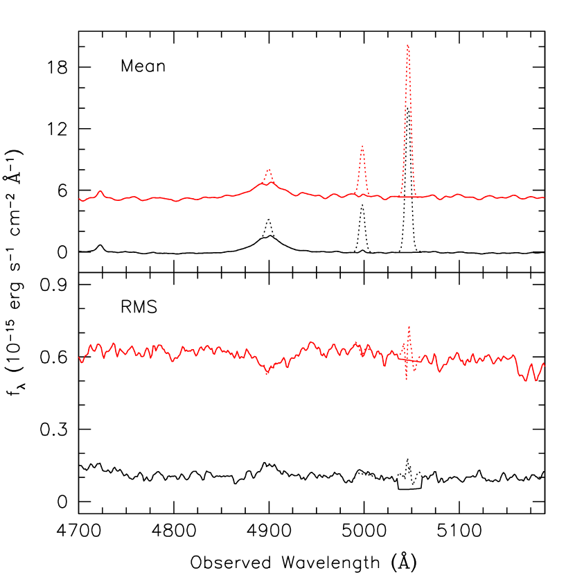
Figure 2.— Top: Mean spectrum of MCG-06-30-15 (red line) and the mean spectrum created after subtraction of the continuum from each individual spectrum (black line). The dotted lines show the narrow component of H$\beta$ and the [O III] $\lambda\lambda$ 4959,5007 doublet. Bottom: RMS of the original calibrated spectra (red line) and rms of the continuum-subtracted spectra (black line). The variable portion of the H$\beta$ emission line is apparent once the strongly variable continuum has been removed.

2.2. Spectroscopy

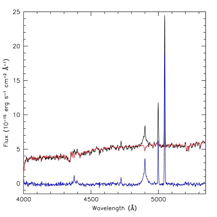
Figure 3.— The black line displays a spectrum of MCG-06-30-15 taken on the night of 1 March 2012, with the best-fit continuum model overplotted in red. The continuum model is comprised of a powerlaw component and a model host-galaxy component. The continuum-subtracted spectrum is plotted in blue.

Spectroscopic monitoring was carried out with RCSpec on the SMARTS 1.5-m telescope at CTIO. Observations were scheduled to be carried out in queue-observing mode every other night during the period 1 March $-$ 31 May 2012. The spectrograph was equipped with the 600 l/mm blue grating (known as grating 26), giving a wavelength coverage of $3685-5400$ Å and a nominal resolution of 1.5 Å pix^-1 in the dispersion direction. Spectra were obtained through a 4″ slit at a fixed position angle of 90° (i.e., oriented east-west). The RCSpec detector, a Loral 1K CCD, provides a spatial resolution of 1$\farcs$3 pix^-1.

Over the course of the campaign, spectra were obtained on 36 nights. Each visit consisted of two spectra with exposure times of 900 s that were obtained at an average airmass of 1.08. A spectrophotometric flux standard, LTT 4364, was also observed during each visit to assist with flux calibrations. Standard reductions were carried out with IRAF and an extraction width of 8 pixels (10$\farcs$4) was adopted.

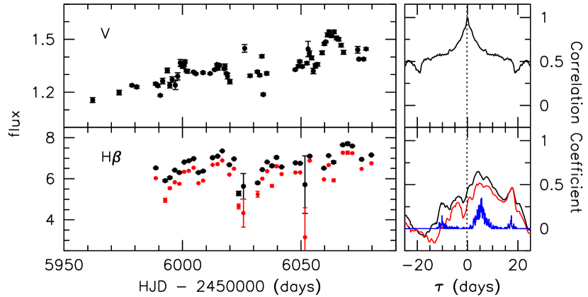
Figure 4.— Continuum light curve (top left) and its autocorrelation function (top right), and the H$\beta$ emission-line (bottom left) light curve and its cross-correlation function relative to the continuum (bottom right). Flux units in the light curves are as listed in Table LABEL:tab:lcdata. In the bottom left panel, the black (red) points show the H$\beta$ emission-line flux measurements based on the continuum-subtracted spectra (original calibrated spectra). The resultant cross-correlation function relative to the continuum light curve for each emission-line light curve is displayed in the same color in the bottom right panel. The H$\beta$ light curves and cross-correlation functions are very similar, demonstrating that our continuum subtraction method does not bias our measurements. In both cases, the emission-line cross-correlation function is an obviously shifted and smoothed version of the continuum auto-correlation function. The blue histogram in the bottom right panel displays the (arbitrarily scaled) cross-correlation centroid distributions based on the continuum light curve and the H$\beta$ light curve measured from the continuum-subtracted spectra, which gives an H$\beta$ time delay of $\tau=5.4\pm 1.8$ days.

The initial flux calibration provided by the standard star is generally a good correction for the shape of the spectra, providing a useful way to remove the effects of the atmospheric transmission as well as the optics of the telescope and instrument. However, reverberation campaigns require high temporal sampling and therefore acquire spectra on all nights when the telescope may be safely used, often times under non-photometric conditions. We therefore require a method for carefully calibrating the overall flux level of each spectrum. This is generally accomplished by using the narrow emission lines as “internal” flux calibration sources, as the narrow lines do not vary on the timescales of a reverberation campaign. Specifically, we employ the van Groningen & Wanders (1992) spectral scaling method with the [O III] $\lambda\lambda$ 4959,5007 emission lines as our internal calibration sources. The method minimizes the differences in a selected wavelength range between each individual spectrum and a reference spectrum created from a subset of the best data. It is therefore able to correct for slight differences in wavelength calibration, slight resolution differences (caused by variable seeing and the employment of a wide spectroscopic slit), as well as flux calibration differences. Peterson et al. (1998a) have shown that this method is able to provide relative spectrophotometry that is accurate to $\sim 2$%. To ensure the accuracy of our absolute spectrophotometry, we compared the integrated [O III] $\lambda 5007$ flux to published values determined from high quality spectra observed under good conditions. We adopted a value of $f($[O III]$)=1.0\times 10^{-13}$ erg s^-1 cm^-2, in good agreement with Morris & Ward (1988), Winkler (1992), and Reynolds et al. (1997).

The red lines in Figure 2 show the mean of all the calibrated spectra throughout the campaign (top) and the root mean square of the spectra (bottom), which highlights variable spectral components. It is immediately obvious that the variable (rms) spectrum is swamped by some combination of host-galaxy light, possibly from mis-centering of the slit and poor seeing conditions, as well as scattered light from a nearby Milky Way star along the line of sight (5$\farcs$4 south of the nucleus and superimposed on the galaxy disk). We therefore investigated a method for carefully subtracting the continuum of each spectrum, both the AGN powerlaw and the starlight, through spectral modeling.

We employed the publicly-available UlySS package (Koleva et al., 2009), which creates a linear combination of non-linear model components convolved with a parametric line-of-sight velocity to match an observed spectrum. Our method started with modeling the very high signal-to-noise mean spectrum. We included a powerlaw component for the AGN continuum emission, multiple Gaussians for the emission lines (three components were necessary to match the H$\beta$ profile), and a host-galaxy component parametrized by the Vazdekis models derived from the MILES library of empirical stellar spectra (Vazdekis et al., 2010). We make no attempt to interpret the best-fit parameters of our model, as our goal was simply to separate the line emission from the continuum components as cleanly as possible. We then held the number of model components and the age and metallicity of the best-fit Vazdekis model fixed, but allowed all other parameters to vary as we looped through all of the individual spectra of MCG-06-30-15. In this way, we allow for variation of the powerlaw index, the relative contribution of powerlaw versus host-galaxy starlight, and emission line flux variability. Furthermore, we modeled the AGN spectra that had an initial flux calibration from a spectrophotometric standard star but had not yet been scaled with the van Groningen & Wanders (1992) code in order to get the best match between the models and the “untouched” observed spectra. The best-fit powerlaw and host-galaxy models were subtracted from each spectrum, providing a set of continuum subtracted, pure emission-line spectra. In Figure 3, we show a typical example of a single spectrum, the best-fit continuum model (powerlaw + starlight), and the resultant continuum-subtracted spectrum.

After modeling and subtraction of the continuum, all the spectra were then scaled with the van Groningen & Wanders (1992) method in the same way as previously described. The mean and rms of the scaled, continuum-subtracted spectra are displayed by the black lines in Figure 2. The H$\beta$ emission line, though weak, is apparent in the continuum-subtracted rms spectrum.

Table 1$V-$band and H$\beta$ Light Curves

HJD	$f_{\lambda}$(V)	HJD	$f$(H$\beta$)
(-2450000)	($10^{-15}$  ergs s-1 cm-2 Å-1)	(-2450000)	($10^{-15}$  ergs s-1 cm-2)
5962.0886	$1.155\pm\ 0.014$	5988.7106	$65.27\pm\ 0.19$
5973.2684	$1.198\pm\ 0.013$	5992.7187	$59.09\pm\ 0.43$
5978.6867	$1.239\pm\ 0.006$	5994.6647	$60.54\pm\ 0.44$
5980.6836	$1.230\pm\ 0.008$	5996.7522	$64.18\pm\ 0.34$
5988.6514	$1.248\pm\ 0.007$	5998.6879	$63.05\pm\ 0.31$
5989.6408	$1.237\pm\ 0.008$	6000.7037	$68.11\pm\ 0.12$
5990.6260	$1.182\pm\ 0.006$	6002.6755	$68.78\pm\ 0.28$
5991.6260	$1.263\pm\ 0.016$	6004.6979	$69.77\pm\ 0.16$
5993.6192	$1.324\pm\ 0.013$	6006.7308	$63.05\pm\ 0.21$
5994.6396	$1.240\pm\ 0.016$	6008.6991	$63.75\pm\ 0.22$
5995.6130	$1.272\pm\ 0.016$	6012.7055	$70.27\pm\ 0.17$
5996.9981	$1.240\pm\ 0.025$	6014.8060	$70.97\pm\ 0.22$
5997.9778	$1.290\pm\ 0.020$	6016.7763	$73.57\pm\ 0.13$
5999.0720	$1.367\pm\ 0.019$	6019.7684	$66.81\pm\ 0.17$
5999.6167	$1.353\pm\ 0.007$	6021.7506	$69.67\pm\ 0.15$
6000.0813	$1.353\pm\ 0.017$	6023.6823	$52.83\pm\ 1.06$
6000.6030	$1.351\pm\ 0.006$	6025.6963	$56.35\pm\ 6.20$
6001.0505	$1.374\pm\ 0.009$	6031.7218	$58.02\pm\ 0.48$
6001.6535	$1.322\pm\ 0.006$	6033.6779	$64.49\pm\ 0.13$
6002.0935	$1.319\pm\ 0.011$	6035.6990	$68.14\pm\ 0.11$
6004.6577	$1.315\pm\ 0.005$	6037.7316	$66.33\pm\ 0.53$
6005.6684	$1.305\pm\ 0.006$	6039.6459	$70.39\pm\ 0.39$
6008.6396	$1.311\pm\ 0.006$	6041.8089	$65.73\pm\ 0.14$
6011.6284	$1.306\pm\ 0.005$	6047.6504	$67.73\pm\ 0.17$
6013.5708	$1.328\pm\ 0.005$	6049.6533	$67.52\pm\ 0.14$
6014.5952	$1.357\pm\ 0.005$	6051.6786	$57.17\pm\ 14.03$
6014.9191	$1.335\pm\ 0.009$	6053.6594	$70.99\pm\ 0.29$
6015.5847	$1.353\pm\ 0.005$	6059.6553	$65.15\pm\ 0.17$
6017.5606	$1.333\pm\ 0.006$	6061.6300	$71.26\pm\ 0.14$
6017.9114	$1.346\pm\ 0.015$	6063.7588	$68.08\pm\ 0.56$
6018.5535	$1.306\pm\ 0.006$	6067.6406	$76.50\pm\ 0.29$
6018.9996	$1.291\pm\ 0.016$	6069.6631	$77.08\pm\ 0.68$
6019.9486	$1.260\pm\ 0.012$	6071.6367	$75.97\pm\ 0.28$
6026.2009	$1.449\pm\ 0.022$	6075.5645	$69.45\pm\ 0.14$
6028.5347	$1.294\pm\ 0.008$	6079.6835	$71.57\pm\ 0.17$
6031.5757	$1.316\pm\ 0.007$
6032.5654	$1.296\pm\ 0.007$
6033.5161	$1.404\pm\ 0.009$
6034.0558	$1.187\pm\ 0.007$
6035.5098	$1.307\pm\ 0.009$
6047.5410	$1.328\pm\ 0.005$
6048.8850	$1.348\pm\ 0.009$
6049.4712	$1.375\pm\ 0.006$
6050.5168	$1.346\pm\ 0.006$
6052.4839	$1.365\pm\ 0.008$
6052.9778	$1.445\pm\ 0.044$
6053.5425	$1.421\pm\ 0.013$
6054.4863	$1.395\pm\ 0.010$
6055.1726	$1.320\pm\ 0.015$
6056.0708	$1.349\pm\ 0.012$
6056.4541	$1.357\pm\ 0.006$
6056.9783	$1.358\pm\ 0.010$
6058.9017	$1.424\pm\ 0.010$
6059.8591	$1.475\pm\ 0.008$
6060.4424	$1.486\pm\ 0.005$
6061.1837	$1.525\pm\ 0.011$
6061.8630	$1.543\pm\ 0.010$
6062.9246	$1.521\pm\ 0.011$
6063.9783	$1.543\pm\ 0.010$
6065.0056	$1.508\pm\ 0.011$
6065.8806	$1.500\pm\ 0.010$
6066.8920	$1.467\pm\ 0.010$
6067.9285	$1.426\pm\ 0.011$
6073.9258	$1.441\pm\ 0.019$
6074.4324	$1.388\pm\ 0.005$
6076.4253	$1.388\pm\ 0.007$
6077.4556	$1.446\pm\ 0.007$

3. Light Curve Analysis

Emission-line light curves were determined from both the original, scaled spectra as well as the continuum-subtracted, scaled spectra, in order to verify that our continuum subtraction method did not introduce artificial variability. In both cases, a local linear continuum was fit underneath the emission line, and the flux above the continuum was integrated. We included this local continuum fit even for the continuum-subtracted spectra to ensure that any small mismatches between the model continuum and that of the spectrum were accounted for and removed from the emission-line measurements. Multiple measurements from a single night were then averaged together to decrease the noise in the resultant light curves, which are displayed in Figure 4. The H$\beta$ light curve derived from the scaled, continuum-subtracted spectra (black points) matches extremely well with the H$\beta$ light curve derived from the scaled-only spectra (red points). The two light curves are virtually identical, with the most obvious difference being a slight offset in which the continuum-subtracted spectra have an elevated H$\beta$ flux (due to correction of the intrinsic H$\beta$ absorption from the starlight). A linear fit to the fluxes determined from each method shows that the difference between the two lightcurves is almost entirely a simple offset, with very minimal flux dependence (close to a slope of 1).

The differential light curves derived from image subtraction analysis of the $V-$band photometry were converted to absolute flux units in the following way. First, the reference image for each set of observations was modeled with the two-dimensional surface brightness fitting program GALFIT. The shape parameters of the galaxy bulge and disk were matched to those derived from the analysis of a high-resolution medium$-V$ Hubble Space Telescope (HST) image (see Section 6.1). Field stars common to both the HST image and the ground-based images were also modeled (circled in Figure 1), and the field star magnitudes derived from the HST image were used to set the absolute flux calibration of the ground-based images. The brightness of the AGN point spread function in each ground-based reference image was then added back to the differential flux derived from the image subtraction analysis for that set of photometry. While the overall flux scale of the light curve is not important, we found a slight offset of 0.2 mag between the FTS and the LT calibrated photometry, so we adjusted the LT photometry to match that of the FTS, since the FTS observations were generally obtained under better conditions. The calibrated photometric light curves were then combined together and measurements coincident within 0.5 days were averaged together. The final $V-$band light curve is displayed in the top left panel of Figure 4.

Table LABEL:tab:lcstats gives the variability statistics for the final $V-$band and H$\beta$ emission-line light curves displayed in Figure 4. Column (1) lists the spectral feature and column (2) gives the number of measurements in the light curve. Columns (3) and (4) list the average and median time separation between measurements, respectively. Column (5) gives the mean flux and standard deviation of the light curve, and column (6) lists the mean fractional error (based on the comparison of observations that are closely spaced in time). Column (7) lists the fractional rms variability amplitude, computed as:

$$F_{\rm var}=\frac{\sqrt{\sigma^{2}-\delta^{2}}}{\langle F\rangle}$$ (1)

where $\sigma^{2}$ is the variance of the fluxes, $\delta^{2}$ is their mean-square uncertainty, and $\langle F\rangle$ is the mean flux (Rodríguez-Pascual et al., 1997). The uncertainty on $F_{\rm var}$ is quantified as

$$\sigma_{F_{\rm var}}=\frac{1}{F_{\rm var}}\sqrt{\frac{1}{2N}}\frac{\sigma^{2}}{\langle F\rangle^{2}}$$ (2)

(Edelson et al., 2002). And column (8) is the ratio of the maximum to the minimum flux in the light curve. At first glance, the $F_{\rm var}$ values for the H$\beta$ light curves from the continuum-subtracted and the unsubtracted spectra appear quite discrepant given the similarities in the light curves. The disagreement arises solely due to two data points in each light curve with large uncertainties, reflecting the marginal conditions under which the observations were obtained. Removal of those two data points from each light curve modifies the $F_{\rm var}$ value for the continuum-subtracted spectra only slightly, increasing from $0.075\pm 0.011$ to $0.080\pm 0.010$. The $F_{\rm var}$ value for the unsubtracted spectra, however, decreases significantly from $0.132\pm 0.018$ to $0.099\pm 0.012$, bringing the $F_{\rm var}$ values for the two light curves into better agreement.

Table 2Light-Curve Statistics

Time Series	$N$	$\langle T\rangle$	$T_{\rm median}$	$\langle F\rangle$	$\langle\sigma_{F}/F\rangle$	$F_{\rm var}$	$R_{\rm max}$
		(days)	(days)
V	67	$1.75\pm\ 2.28$	1.00	$1.35\pm\ 0.09$	0.008	$0.066\pm\ 0.006$	$1.336\pm\ 0.018$
H$\beta$, non-CS	35	$2.68\pm\ 1.26$	2.02	$6.10\pm\ 0.85$	0.023	$0.132\pm\ 0.018$	$2.306\pm\ 1.053$
H$\beta$, CS	35	$2.68\pm\ 1.26$	2.02	$6.68\pm\ 0.57$	0.014	$0.075\pm\ 0.011$	$1.459\pm\ 0.032$

To determine the mean time delay of the H$\beta$ emission line relative to the continuum variations, we cross correlated the H$\beta$ light curve derived from the continuum-subtracted spectra (Figure 4, black points) with the $V-$band light curve (both tabulated in Table LABEL:tab:lcdata). We employed the interpolated cross-correlation function (ICCF) method (Gaskell & Sparke, 1986; Gaskell & Peterson, 1987) with the modifications of White & Peterson (1994). This method determines the cross-correlation function (CCF) twice, by first interpolating the continuum light curve and then by interpolating the emission-line light curve in the second pass. The resultant CCF, which is the average of the two, is shown by the black solid line in the bottom right panel of Figure 4. For reference, we calculated the autocorrelation function of the $V-$band light curve, displayed by the solid line in the top right panel of Figure 4. Also displayed in Figure 4 is the CCF for the H$\beta$ light curve derived from the original, scaled spectra (red points) compared to the $V-$band (red line). As expected given the nearly identical variations in the H$\beta$ light curves, the cross correlation functions of the two relative to $V$ are also nearly identical. However, the slightly reduced noise in the H$\beta$ light curve derived from the continuum-subtracted spectra provides a higher correlation coefficient at the preferred time delay. We therefore focus the remainder of our analysis on the H$\beta$ light curve derived from the continuum-subtracted spectra.

CCFs can be characterized by their maximum value ($r_{\rm max}$), the time delay at which the CCF maximum occurs ($\tau_{\rm peak}$), and the centroid of the points near the peak ($\tau_{\rm cent}$) above a threshold value of $0.8r_{\rm max}$. However, a single CCF does not provide any information on the uncertainties inherent in these measurements. We therefore employ the “flux randomization/random subset sampling” (FR/RSS) method of Peterson et al. (1998b, 2004), which is a Monte Carlo approach for determining the uncertainties in our measured time delays. For a sample of $N$ data points, a selection of $N$ points is chosen without regard to whether a datum was previously chosen or not. The typical number of points that is not sampled in a single realization is $\sim 1/e$. A point that is sampled $1\leq n\leq N$ times has its uncertainty reduced by a factor of $n^{1/2}$. This “random subset sampling” step is therefore able to assess the uncertainty in the time delay that arises from an individual data point in the light curve. The “flux randomization” step takes each of the selected points and modifies the flux value by a Gaussian deviation of the uncertainty. In this way, the effect of the measurement uncertainties on the recovered time delay is also assessed. The final modified light curves are then cross correlated with the ICCF method described above, and the values of $r_{\rm max}$, $\tau_{\rm peak}$, and $\tau_{\rm cent}$ are recorded. The entire process is repeated 1000 times, and distributions of these values are built up from all of the realizations. We take the medians of the cross-correlation peak distribution (CCPD) and the cross-correlation centroid distribution (CCCD) as $\tau_{\rm peak}$ and $\tau_{\rm cent}$, respectively. The uncertainties on these values are quoted so that 15.87% of the realizations fall above and 15.87% fall below the range of uncertainties, corresponding to $\pm 1\sigma$ for a Gaussian distribution. The final measurements are quoted in Table LABEL:tab:lagwidth in both the observer’s frame and the rest frame of the AGN, and the CCCD is displayed in the bottom right panel of Figure 4 as the blue histogram (arbitrarily scaled). The mean of the distribution agrees well with the time delay inferred from the CCF.

For comparison, we also determined the H$\beta$ time delay using the JAVELIN code (Zu et al., 2011). JAVELIN employs a damped random walk to model the continuum variations, and then determines the best reprocessing model by quantifying the shifting and smoothing parameters necessary to reproduce the emission-line light curve (see Figure 5). The uncertainties on the model parameters are assessed through a Bayesian Markov Chain Monte Carlo method. We include the JAVELIN time delay as $\tau_{\rm jav}$ in Table LABEL:tab:lagwidth.

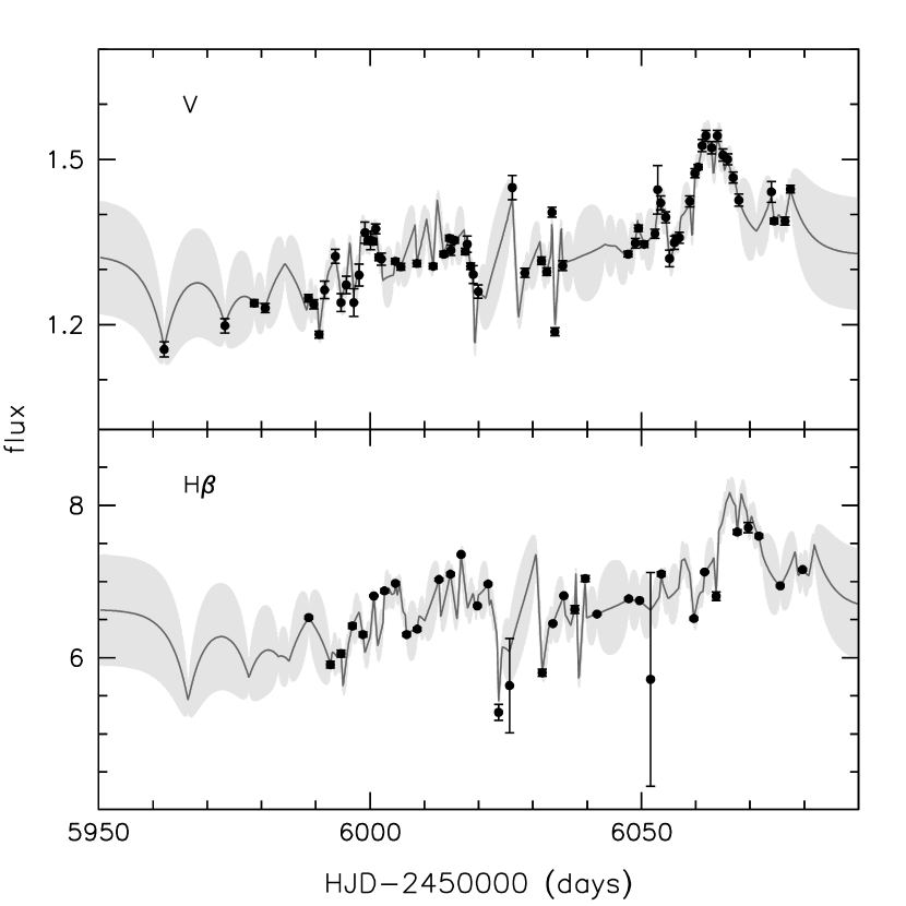
Figure 5.— $V-$band light curve (data points, top) and H$\beta$ light curve derived from the continuum-subtracted spectra (data points, bottom). The mean JAVELIN models and uncertainties are overplotted as the solid lines and gray shaded regions, respectively. The model uncertainties are derived from the standard deviation of the individual realizations. JAVELIN finds a best-fit H$\beta$ time delay of $4.4\pm 0.1$ days.

Additionally, we used a Markov Chain Monte Carlo code MCMCRev to fit a linearised echo model to the $V-$band and H$\beta$ lightcurves (see Figure 6). This models the $V-$band lightcurve with a fourier series constrained by the lightcurve data and with a random-walk prior that mimics typical AGN continuum variations on $1-100$ d timescales. H$\beta$ variations are modeled as an echo of those in the $V$ band. A two-parameter delay distribution, specifically

$$\Psi(\tau)=\frac{\Psi_{0}}{2\,\tau_{0}}\frac{(\tau/\tau_{0})^{9/4}}{\cosh{(\tau/\tau_{0})}-1}\ ,$$ (3)

enforces causality ($\tau>0$) and has a width proportional to the mean delay $\langle\tau\rangle\approx 5\,\tau_{0}$. Three further parameters are the mean H$\beta$ flux, and two factors that scale the nominal H$\beta$ and V-band error bars. The mean and rms of the MCMC samples give the H$\beta$ delay as $\langle\tau\rangle=4.6\pm 2.8$ days, in agreement with the other techniques.

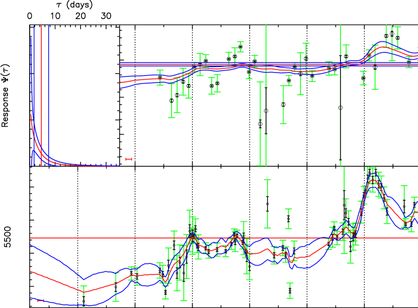
Figure 6.— Results of the MCMCRev fit of a linearised echo model to the H$\beta$ (top) and V-band (bottom) lightcurve data. The red and blue curves give the mean $\pm$ rms over MCMC samples of the model lightcurves and the delay distribution (top left). The mean and rms of MCMC samples give the mean H$\beta$ delay as $\langle\tau\rangle=4.6\pm 2.8$ days.

Table 3Time Lags and Line Widths

Frame	$\tau_{\rm cent}$	$\tau_{\rm peak}$	$\tau_{\rm jav}$	Spectrum	FWHM	$\sigma_{\rm line}$
	(days)	(days)	(days)		(km s-1)	(km s-1)
Observed	$5.37^{+1.87}_{-1.76}$	$4.40^{+3.10}_{-0.80}$	$4.40^{+0.08}_{-0.10}$	Mean	$1958.4\pm\ 74.8$	$975.6\pm\ 8.4$
Rest-frame	$5.33^{+1.86}_{-1.75}$	$4.37^{+3.08}_{-0.79}$	$4.37^{+0.08}_{-0.10}$	RMS	$1422.0\pm\ 416.4$	$664.5\pm\ 87.3$

4. Line Width Measurements

The broad emission lines in AGN spectra are interpreted as being Doppler broadened through the bulk gas motions deep in the potential well of the black hole. Therefore, the width of the broad line is a constraint on the line-of-sight velocity of the gas. The narrow emission lines, however, are produced by gas that is well outside the nucleus of the AGN and does not reverberate on the time scales of a few months. It is therefore important that we remove the narrow contribution to the H$\beta$ emission line before attempting to measure the line width.

We accomplish this by using the [O III] $\lambda$5007 emission line as a template for the narrow emission lines in the spectrum. The template is shifted and scaled by an appropriate amount to account for both the [O III] $\lambda$4959 line and the H$\beta$ narrow line. We adopted a scale factor of $\lambda 4959/\lambda 5007=0.34$ (Storey & Zeippen, 2000) and, through trial and error, determined a scale factor of H$\beta$/$\lambda 5007=0.10$. The original and narrow-line subtracted spectra are displayed in Figure 2.

From the narrow-line subtracted spectra, we determined the emission line width in both the mean and rms of the continuum-subtracted spectra. A local linear continuum was determined from two continuum windows on either side of the emission line, and the width was determined directly from the measurements above this local continuum. We report the line width as the full width at half the maximum flux (FWHM) and also as the second moment of the line profile, or the line dispersion, $\sigma_{\rm line}$.

The uncertainties on the line width measurements were determined from a Monte Carlo random subset sampling method. For a set of $N$ spectra, we select $N$ without regard to whether a spectrum was previously chosen or not. The mean and rms of this subset are determined, and the FWHM and $\sigma_{\rm line}$ are tabulated. The process is repeated 1000 times, and a distribution of each measurement is built up. In this way, the effect of any particular spectrum on the line width measurements is assessed. We also included a slight modification in which the continuum windows on either side of the emission line were allowed to vary in size and exact placement within an acceptable range, thereby assessing the effect of the continuum window choice on the final measurements. This modification generally has little or no effect on the line widths derived from the rms spectrum, where noise already dominates the uncertainties, but slightly increases the uncertainties on the line widths derived from the mean spectrum (Bentz et al., 2009b). The mean and standard deviation of each distribution are adopted as the measurement value and its uncertainty, respectively.

Finally, we also corrected for the dispersion of the spectrograph following the method employed by Peterson et al. (2004), in which the observed line width can be described as a combination of the intrinsic line width, $\Delta\lambda_{\rm true}$, and the spectrograph dispersion, $\Delta\lambda_{\rm disp}$, such that

$$\Delta\lambda_{\rm obs}^{2}\approx\Delta\lambda_{\rm true}^{2}+\Delta\lambda_{\rm disp}^{2}.$$ (4)

In this case, it is not possible to measure $\Delta\lambda_{\rm disp}$ from sky lines or arc lamps employed for wavelength calibration, because in both of those cases, the source fills the entire slit. However, the angular size of the unresolved AGN point source is set by the seeing, which varies throughout the campaign but is almost always smaller than the 5″ width of the slit. Our typical approach is to therefore search the literature for very high resolution measurements of the width of the [O III] lines, to serve as a measurement of $\Delta\lambda_{\rm true}$, allowing $\Delta\lambda_{\rm disp}$ to be determined. Such measurements do not exist for MCG-06-30-15, but they do exist for NGC 1566, another Seyfert galaxy that we have monitored with the same instrument and setup.

For NGC 1566, Whittle (1992) measured ${\rm FWHM}=280$ km s^-1 for [O III] $\lambda 5007$ through a small slit, with a high resolution, and under good observing conditions. From our own spectra of NGC 1566 taken with RCSpec on the SMARTS 1.5-m telescope, we determined ${\rm FWHM}=8.26$ Å for [O III] $\lambda 5007$. We therefore deduce a value of $\Delta\lambda_{\rm disp}=6.8$ Å and adopt this value for our observations of MCG-06-30-15. The final dispersion-corrected line widths and uncertainties for the mean and rms H$\beta$ broad line profiles are tabulated in Table LABEL:tab:lagwidth.

5. Black Hole Mass

The black hole mass is generally derived from reverberation-mapping measurements as

$$M_{BH}=f\frac{RV^{2}}{G}$$ (5)

where $R$ is taken to be $c\tau$, the speed of light times the mean time delay of a broad emission line relative to continuum variations, $V$ is the line-of-sight velocity of the gas in the broad line region and is determined from the emission line width, and $G$ is the gravitational constant.

The factor $f$ is a scaling factor that accounts for the detailed geometry and kinematics of the gas in the broad line region, which is generally unknown. In practice, it has become common to determine the population average multiplicative factor, $\langle f\rangle$, necessary to bring the $M_{\rm BH}-\sigma_{\star}$ relationship for AGNs with reverberation masses into agreement with the $M_{\rm BH}-\sigma_{\star}$ relationship for nearby galaxies with dynamical black hole masses (e.g., Gültekin et al. 2009; McConnell & Ma 2013; Kormendy & Ho 2013). In this way, the overall scale for reverberation masses should be unbiased, but the mass of any single AGN is expected to be uncertain by a factor of 2-3. The value of $\langle f\rangle$ has varied in the literature from 5.5 (Onken et al., 2004) to 2.8 (Graham et al., 2011), depending on which objects are included and the specifics of the measurements. We adopt the value determined by Grier et al. (2013) of $\langle f\rangle=4.3\pm 1.1$.

Our preferred combination of measurements is $\tau_{\rm cent}$ for the time delay and $\sigma_{\rm line}$ measured from the rms spectrum for the line width. Combined with our adopted value of $\langle f\rangle$, we determine a black hole mass of $(1.6\pm 0.4)\times 10^{6}$ M_⊙ for MCG-06-30-15.

6. Discussion

We present here the first optical emission-line reverberation results for MCG-06-30-15, but the well-studied nature of this AGN ensures that we have ample comparisons available in the literature with which we can assess our results. Lira et al. (2015) describe a long-term monitoring campaign in X-ray, optical, and near-IR bands from which several broad-band time delays were measured. In particular, they find that the near-IR bands lag the $B$ and $V$ bands by 13, 20, and 26 days in $J$, $H$, and $K$ respectively. While our monitoring campaign was not contemporaneous with that described by Lira et al. (2015), it was carried out the following observing season. Furthermore, Kara et al. (2014) find that the luminosity state of MCG-06-30-15 did not change significantly over the period between 2001 and 2013, and the light curve from the Swift/BAT hard X-ray transient monitor shows no luminosity state changes between 2005 and 2015 (Krimm et al., 2013). Comparison of our measured H$\beta$ time delay of $\tau_{\rm cent}=5.3\pm\ 1.8$ days to the near-IR delays places the inner edge of the dust torus outside the BLR, as has been found for other Seyferts (Clavel et al., 1989; Suganuma et al., 2006; Koshida et al., 2014). Furthermore, our H$\beta$ time delay compares remarkably well with the findings of Koshida et al. (2014) that $\tau(K)/\tau({\rm H}\beta)\approx 4-5$. These findings are also in keeping with the scenario proposed by Netzer & Laor (1993) in which the dust torus creates the outer edge of the BLR through suppression of line emission by the dust grains.

6.1. AGN Radius$-$Luminosity Relationship

The empirical relationship between the AGN BLR radius and the AGN optical luminosity (Kaspi et al., 2000, 2005; Bentz et al., 2006, 2009a, 2013) is a well-known scaling relationship derived from the set of reverberation mapping measurements for relatively nearby AGNs. The calibrated relationship relies on H$\beta$ reverberation results and measurements of the continuum luminosity at 5100 Å, and it provides a quick way to estimate black hole masses without investing in time- and resource-intensive reverberation mapping programs for every target of interest. The $R_{\rm BLR}$–$L$ relationship has been found to be in good agreement with simple expectations from photoionization physics, once the luminosity measurements were corrected for the host-galaxy starlight contribution measured through the reverberation-mapping spectroscopic aperture (Bentz et al., 2006, 2009a, 2013). The scatter has also been found to be quite low, $<0.2$ dex (Bentz et al., 2013), implying that AGNs are mostly luminosity-scaled versions of each other.

Starlight corrections are especially important for nearby AGNs, like MCG-06-30-15, because they can provide a significant fraction of the flux through the reverberation-mapping spectroscopic aperture. These corrections are generally obtained through two-dimensional surface brightness modeling of high-resolution AGN host galaxy images. The decomposition allows the AGN PSF to be accurately separated from the host-galaxy and the underlying sky, and thus an “AGN free” image can be recovered from which the starlight flux can be measured. MCG-06-30-15 was observed with HST and the UVIS channel of WFC3 through the F547M filter as part of program GO-11662 to image the host galaxies of the LAMP 2008 AGN sample (Bentz et al., 2013). A single orbit was split into two pointings separated by a small angle maneuver, and at each pointing a set of three exposures was taken, each exposure graduated in exposure time (short, medium, and long). The saturated pixels in the AGN core in the long exposures are corrected by scaling up the same pixels from the shorter, unsaturated exposures by the ratio of the exposure times. In this way, the graduated exposure times allow the dynamic range of the final drizzled image to significantly exceed the dynamic range of the detector itself. The total exposure time of the final combined, drizzled image is 2290 s.

Two-dimensional surface brightness fitting of the HST image was carried out with the GALFIT software (Peng et al., 2002, 2010). We fit the host-galaxy of MCG-06-30-15 with a Sérsic bulge and an exponential disk with an inner radial (truncation) function to approximate the dust lane. A single Fourier mode ($m=1$) was also allowed for each of these components, to account for gross perturbations on the initial parametric models. The AGN and nearby star were fit with a model PSF generated by the Starfit algorithm (Hamilton, 2014), which starts with a TinyTim PSF model (Krist, 1993) and then fits the subpixel centering and the telescope focus. The underlying sky background was also fit as a gradient, and we used the entire field of view provided by WFC3 to ensure that it was properly constrained, even though the galaxy itself only covers a small portion of the UVIS1 camera. The parameters for our best-fit model are tabulated in Table LABEL:tab:galfit, and Figure 7 displays a region of the HST image centered on the galaxy (left), the best-fit model image (center), and the residuals after subtraction of the model from the image (right).

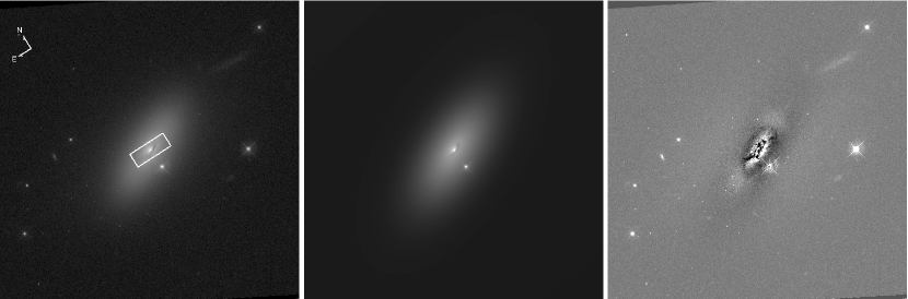
Figure 7.— Left: HST image of the host-galaxy of MCG-06-30-15, displayed with a logarithmic stretch. The scale of is 80″ $\times$80″and is only a portion of the full field of view. The white rectangle centered on the galaxy nucleus shows the ground-based spectroscopic monitoring aperture. Middle: GALFIT model, displayed with the same stretch as the image. Right: Residuals after subtracting the model from the image, displayed with a linear stretch centered around zero counts.

Table 4Surface Brightness Decomposition

#	PSF+sky	$\Delta x$ (″)	$\Delta y$ (″)	$m_{\rm stmag}$	…	Sky (cts)	$\frac{d{\rm sky}}{dx}$ ($10^{-4}$ cts)	$\frac{d{\rm sky}}{dy}$ ($10^{-4}$ cts)	Note
	sersic	$\Delta x$ (″)	$\Delta y$ (″)	$m_{\rm stmag}$	$r_{\rm e}$ (″)	$n$	$b/a$	PA (deg)
	sersic3	$\Delta x$ (″)	$\Delta y$ (″)	$\Sigma_{\rm stmag}$	$r_{\rm e}$ (″)	$n$	$b/a$	PA (deg)
	radial	$\Delta x$ (″)	$\Delta y$ (″)	$\cdots$	$r_{\rm break}$ (″)	$\Delta r_{\rm soft}$ (″)	$b/a$	PA (deg)
	fourier	$\cdots$	mode: $a_{\rm m}$ , $\phi$ (deg)		$\cdots$	$\cdots$	$\cdots$	$\cdots$
(1)	(2)	(3)	(4)	(5)	(6)	(7)	(8)	(9)	(10)
1,2	PSF+sky	0.000	0.000	16.26	$\cdots$	31.72	-3.7	4.2
3	sersic	0.038	-0.008	15.70	1.014	1.9	0.47	-36.8	bulge
	fourier	1: -0.418	-96.2
4	sersic3	0.132	-0.092	18.66	8.216	[1.0]	0.48	-32.1	disk
	radial,inner	1.036	0.764	$\cdots$	2.149	2.195	0.35	-24.7	dust lane
	fourier	1: 0.722	116.5
merit		$\chi^{2}=645340672.0$			$N_{\rm dof}=15783039$		$N_{\rm free}$=29	$\chi^{2}_{\nu}=40.88$

Note. — Values in square brackets were held fixed during the surface brightness model fitting.

Using our best-fit model, we created a sky- and AGN-subtracted image of MCG-06-30-15. From this image, we measured the host-galaxy flux density through the ground-based spectroscopic monitoring aperture (depicted as the white rectangle in the left panel of Figure 7). The scaling factor necessary to correct the flux density from the effective wavelength of the HST filter to 5100$\times$(1+z) was determined with synphot and a template galaxy bulge spectrum (Kinney et al., 1996). Our determination of the host-galaxy flux density at 5100$\times$(1+z) is $f_{\rm gal}=(4.28\pm 0.43)\times 10^{-15}$ erg s^-1 cm^-2 Å^-1. The average flux density at 5100$\times$(1+z) was determined from our scaled spectra to be $f_{\rm obs}=(5.23\pm 0.08)\times 10^{-15}$ erg s^-1 cm^-2 Å^-1. Correcting for the host-galaxy contribution, we deduce an AGN-only flux density of $f_{\rm AGN}=(0.95\pm 0.49)\times 10^{-15}$ erg s^-1 cm^-2 Å^-1.

Unfortunately, the distance to MCG-06-30-15 is not particularly well constrained. The luminosity distance implied by the galaxy redshift is $D_{L}=32.5$ Mpc. However, the Extragalactic Distance Database (Tully et al., 2009) reports $D=25.5\pm 3.5$ from their cosmic flows model and the group membership of MCG-06-30-15 (Tully et al., 2013). Taken at face value, this $\sim 30$% disagreement in distance leads to a factor of 1.6 uncertainty in the luminosity. Additionally, there are only three galaxies contributing to the group distance determination, and the individual distance estimates for these three galaxies range from $20-36$ Mpc. As part of a separate program to determine Tully & Fisher (1977) distances to AGN host galaxies, we observed MCG-06-30-15 with the Green Bank Telescope, but we were unable to detect H I 21 cm emission with 3.5 hrs of on-source time. For our purposes here, we adopt the cosmic flows estimate and its uncertainty, but we note that it will be important to better constrain the distance to this galaxy in order to determine more accurate physical parameters (including, but not limited to, any luminosity measurements). After correcting for Galactic extinction along the line of sight as determined by Schlafly & Finkbeiner (2011), we find $\log\lambda L_{\lambda}(5100\,{\rm\AA})=41.65\pm 0.25$ erg s^-1.

Figure 8 depicts the location of MCG-06-30-15 on the $R_{\rm BLR}$–$L$ relationship. We have not determined a new best fit to the relationship, but have simply recreated the plot from Bentz et al. (2013). MCG-06-30-15 is fairly consistent with the typical scatter around the relationship. We note that if we were to adopt one of the other time delay measurements (such as $\tau_{\rm jav}$), or the luminosity distance from the galaxy redshift, the agreement would be even better. With the adopted assumptions, and furthermore assuming that $L_{\rm bol}=4.9+0.9\lambda L_{\lambda}(5100\,{\rm\AA})$ (Runnoe et al., 2012), we estimate $L/L_{\rm Edd}=0.04$.

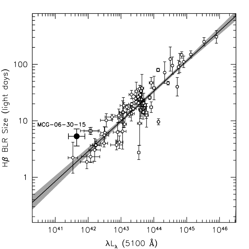
Figure 8.— The radius$-$luminosity relationship for AGNs (open points and fit; Bentz et al. 2013) with the H$\beta$ time delay and AGN luminosity for MCG-06-30-15 from this work plotted as the filled point.

6.2. Black Hole Mass Consistency

Our measurement of $M_{\rm BH}=(1.6\pm 0.4)\times 10^{6}$ M_⊙ for MCG-06-30-15 is in excellent agreement with the value determined by McHardy et al. (2005) of $M_{\rm BH}=2.9^{+1.8}_{-1.6}\times 10^{6}$ M_⊙. Their work assumed a linear scaling between $M_{\rm BH}$ and the X-ray power spectral density break, with the relationship anchored to the measurements for the Galactic black hole Cygnus X-1. This agreement therefore bolsters the claim that supermassive black holes are simply analogs of Galactic black holes, but scaled up in mass (e.g., McHardy et al. 2006).

Raimundo et al. (2013) describe VLT SINFONI integral field spectroscopic observations of the innermost $\sim 0.5$ kpc of the galaxy in the $H$ band. Although their observations were somewhat shallow (total on-source exposure time of 1.3 hours), they attempted to constrain the black hole mass with the Jeans Anisotropic Model method (Cappellari, 2008). Intriguingly, they find a best-fit value of $M_{\rm BH}=4\times 10^{6}$ M_⊙ (assuming $D=37$ Mpc), although they caution that there is actually a stronger constraint on an upper limit of $M_{\rm BH}<6\times 10^{7}$ M_⊙ than on the best-fit mass.

One of our original reasons for targeting MCG-06-30-15 included the fact that it might be possible to determine a black hole mass through both reverberation mapping and stellar dynamical modeling for this nearby AGN. The sample of objects for which we are able to compare these two mass determination methods is extremely small for two reasons: (1) stellar dynamical modeling is limited by spatial resolution, and therefore distance; and (2) broad-lined AGNs in the local Universe are quite rare, and therefore generally far away. Only two galaxies have published masses from both methods thus far — NGC 4151 (Bentz et al., 2006; Onken et al., 2014) and NGC 3227 (Davies et al., 2006; Denney et al., 2010).

A useful metric for determining whether a stellar dynamical mass is likely to be achievable is to determine whether the black hole sphere of influence ($r_{h}$) could be resolved with the observations, where

$$r_{h}=\frac{GM_{BH}}{\sigma_{\star}^{2}}.$$ (6)

Combining our mass with the value of $\sigma_{\star}=109$ km s^-1 determined by Raimundo et al. (2013) and the distance of 25.5 Mpc adopted above, we estimate $r_{h}=0.005$″. This scale is not resolvable with currently-available instruments, although Gültekin et al. (2009) argue that it is not strictly necessary to resolve $r_{h}$ to obtain a useful constraint on $M_{\rm BH}$. Furthermore, the best-fit black hole mass derived by Raimundo et al. (2013), even with shallow observations and a spatial scale of 0.05″, suggests that it could be worthwhile to pursue a stellar dynamical mass constraint for MCG-06-30-15. In this case, an accurate distance will be even more necessary, as dynamical masses scale linearly with the assumed distance.

Time lags between different X-ray energy bands have also been detected in MCG-06-30-15 (Emmanoulopoulos et al., 2011; De Marco et al., 2013; Kara et al., 2014). Of particular interest are soft X-ray lags (where low energy X-rays lag behind higher energy X-rays), likely due to X-ray reverberation (Fabian et al., 2009). Emmanoulopoulos et al. (2011) first detected a soft lag of approximately 20 s in MCG-06-30-15. A systematic search for, and analysis of, soft lags in X-ray variable AGN found that the amplitude of the soft lags and Fourier frequency where they are observed scales with black hole mass (De Marco et al., 2013). MCG-06-30-15 is one of the 15 soft lag detections used to determine the scaling relation, with a black hole mass estimated from the $R_{\rm BLR}$–$L$ relationship. Ignoring that MCG-06-30-15 was used in determined the soft lag scaling relation, and that the scaling relation is subject to selection biases (De Marco et al., 2013), we can use the soft lag to estimate the black hole mass. De Marco et al. (2013) measure a soft lag of $26.4\pm 12.7$ s, which predicts a black hole mass of $1.1\times 10^{6}$ M_⊙, consistent with the reverberation mass we have determined in this work.

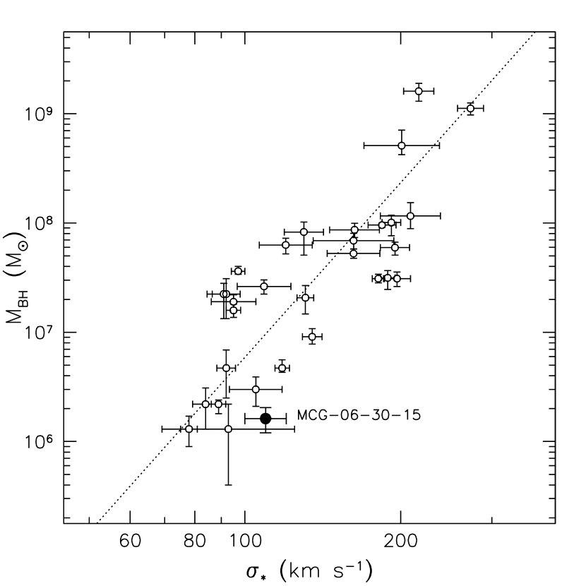
Figure 9.— The $M_{\rm BH}-\sigma_{\star}$ relationship for AGNs (open points and fit; Grier et al. 2013) with MCG-06-30-15 plotted as the filled point.

6.3. AGN $M-\sigma$ Relationship

We also examine the black hole mass we have derived for MCG-06-30-15 in light of the $M_{\rm BH}-\sigma_{\star}$ relationship for other AGNs with reverberation masses. Raimundo et al. (2013) contrained the bulge stellar velocity dispersion from their VLT SINFONI velocity dispersion maps using a pseudoslit geometry and determined $\sigma_{\star}=109$ km s^-1. This value is somewhat larger than the value of $\sigma_{\star}=93.5\pm 8.5$ km s^-1 determined by McHardy et al. (2006) from longslit spectroscopy.

In Figure 9, we show the AGN $M_{\rm BH}-\sigma_{\star}$ relationship from Grier et al. (2013). MCG-06-30-15 sits a bit below and to the right of the relationship, but appears to be fairly consistent within the scatter. Adoption of the McHardy et al. (2006) value of $\sigma_{\star}$ would further bolster the agreement.

We note that we have an independent project currently in progress that will recalibrate the AGN $M_{\rm BH}-\sigma_{\star}$ relationship using velocity dispersions derived solely from integral field spectroscopy, which will be important for removing any rotational broadening effects from the $\sigma_{\star}$ measurements among the rest of the sample (Batiste & Bentz, 2016), as well as any scatter imposed by the selection of a specific position angle for longslit observations. We intend to revisit the location of MCG-06-30-15 on this relationship at that time.

7. Summary

We have determined a reverberation time delay for the broad H$\beta$ emission line in the spectrum of MGC-06-30-15 of $\tau_{\rm cent}=5.3\pm 1.8$ days in the rest-frame of the AGN. The measured time delay is in good agreement with the AGN $R_{\rm BLR}$–$L$ relationship. It also agrees with the relationship between H$\beta$ and near-IR time delays, where the effective optical BLR size is approximately 4-5 times smaller than the inner edge of the dust torus. Combining the H$\beta$ time delay measurement with the width of the emission line in the variable part of the spectrum, we constrain a central black hole mass of $M_{\rm BH}=(1.6\pm 0.4)\times 10^{6}$ M_⊙. This value is in good agreement with estimates from the X-ray power spectral density break and $M_{\rm BH}-\sigma_{\star}$ relationships.

References

- Alard (2000) Alard, C. 2000, A&AS, 144, 363
- Alard & Lupton (1998) Alard, C., & Lupton, R. H. 1998, ApJ, 503, 325
- Antonucci (1993) Antonucci, R. 1993, ARA&A, 31, 473
- Batiste & Bentz (2016) Batiste, M., & Bentz, M. C. 2016, in American Astronomical Society Meeting Abstracts, Vol. 227, American Astronomical Society Meeting Abstracts, 104.07
- Bentz et al. (2013) Bentz, M. C., Denney, K. D., Grier, C. J., et al. 2013, ApJ, 767, 149
- Bentz et al. (2009a) Bentz, M. C., Peterson, B. M., Netzer, H., Pogge, R. W., & Vestergaard, M. 2009a, ApJ, 697, 160
- Bentz et al. (2006) Bentz, M. C., Peterson, B. M., Pogge, R. W., Vestergaard, M., & Onken, C. A. 2006, ApJ, 644, 133
- Bentz et al. (2009b) Bentz, M. C., Walsh, J. L., Barth, A. J., et al. 2009b, ApJ, 705, 199
- Bentz et al. (2008) Bentz, M. C., et al. 2008, ApJ, 689, L21
- Blandford & McKee (1982) Blandford, R. D., & McKee, C. F. 1982, ApJ, 255, 419
- Brenneman & Reynolds (2006) Brenneman, L. W., & Reynolds, C. S. 2006, ApJ, 652, 1028
- Cappellari (2008) Cappellari, M. 2008, MNRAS, 390, 71
- Chiang & Fabian (2011) Chiang, C.-Y., & Fabian, A. C. 2011, MNRAS, 414, 2345
- Clavel et al. (1989) Clavel, J., Wamsteker, W., & Glass, I. S. 1989, ApJ, 337, 236
- Davies et al. (2006) Davies, R. I., Thomas, J., Genzel, R., et al. 2006, ApJ, 646, 754
- De Marco et al. (2013) De Marco, B., Ponti, G., Cappi, M., Dadina, M., Uttley, P., Cackett, E. M., Fabian, A. C., & Miniutti, G. 2013, MNRAS, 431, 2441
- Denney et al. (2010) Denney, K. D., Peterson, B. M., Pogge, R. W., et al. 2010, ApJ, 721, 715
- Edelson et al. (2002) Edelson, R., Turner, T. J., Pounds, K., Vaughan, S., Markowitz, A., Marshall, H., Dobbie, P., & Warwick, R. 2002, ApJ, 568, 610
- Emmanoulopoulos et al. (2011) Emmanoulopoulos, D., McHardy, I. M., & Papadakis, I. E. 2011, MNRAS, 416, L94
- Fabian (2012) Fabian, A. C. 2012, ARA&A, 50, 455
- Fabian et al. (2009) Fabian, A. C., Zoghbi, A., Ross, R. R., et al. 2009, Nature, 459, 540
- Fath (1913) Fath, E. A. 1913, ApJ, 37
- Ferrarese & Ford (2005) Ferrarese, L., & Ford, H. 2005, Space Sci. Rev., 116, 523
- Ferrarese & Merritt (2000) Ferrarese, L., & Merritt, D. 2000, ApJ, 539, L9
- Gaskell & Peterson (1987) Gaskell, C. M., & Peterson, B. M. 1987, ApJS, 65, 1
- Gaskell & Sparke (1986) Gaskell, C. M., & Sparke, L. S. 1986, ApJ, 305, 175
- Gebhardt et al. (2000) Gebhardt, K., Bender, R., Bower, G., et al. 2000, ApJ, 539, L13
- Graham et al. (2011) Graham, A. W., Onken, C. A., Athanassoula, E., & Combes, F. 2011, MNRAS, 412, 2211
- Grier et al. (2013) Grier, C. J., Martini, P., Watson, L. C., et al. 2013, ApJ, 773, 90
- Grier et al. (2012) Grier, C. J., Peterson, B. M., Pogge, R. W., et al. 2012, ApJ, 755, 60
- Gültekin et al. (2009) Gültekin, K., Richstone, D. O., Gebhardt, K., et al. 2009, ApJ, 698, 198
- Hamilton (2014) Hamilton, T. S. 2014, in American Astronomical Society Meeting Abstracts, Vol. 223, American Astronomical Society Meeting Abstracts #223, 145.02
- Heckman & Best (2014) Heckman, T. M., & Best, P. N. 2014, ARA&A, 52, 589
- Kara et al. (2014) Kara, E., Fabian, A. C., Marinucci, A., Matt, G., Parker, M. L., Alston, W., Brenneman, L. W., Cackett, E. M., & Miniutti, G. 2014, MNRAS, 445, 56
- Kaspi et al. (2005) Kaspi, S., Maoz, D., Netzer, H., Peterson, B. M., Vestergaard, M., & Jannuzi, B. T. 2005, ApJ, 629, 61
- Kaspi et al. (2000) Kaspi, S., Smith, P. S., Netzer, H., Maoz, D., Jannuzi, B. T., & Giveon, U. 2000, ApJ, 533, 631
- King & Pounds (2015) King, A., & Pounds, K. 2015, ARA&A, 53, 115
- Kinney et al. (1996) Kinney, A. L., Calzetti, D., Bohlin, R. C., McQuade, K., Storchi-Bergmann, T., & Schmitt, H. R. 1996, ApJ, 467, 38
- Koleva et al. (2009) Koleva, M., Prugniel, P., Bouchard, A., & Wu, Y. 2009, A&A, 501, 1269
- Kormendy & Ho (2013) Kormendy, J., & Ho, L. C. 2013, ARA&A, 51, 511
- Koshida et al. (2014) Koshida, S., Minezaki, T., Yoshii, Y., et al. 2014, ApJ, 788, 159
- Krawczynski & Treister (2013) Krawczynski, H., & Treister, E. 2013, Frontiers of Physics, 8, 609
- Krimm et al. (2013) Krimm, H. A., Holland, S. T., Corbet, R. H. D., et al. 2013, ApJS, 209, 14
- Krist (1993) Krist, J. 1993, in ASP Conf. Ser. 52: Astronomical Data Analysis Software and Systems II, 536
- Lira et al. (2015) Lira, P., Arévalo, P., Uttley, P., McHardy, I. M. M., & Videla, L. 2015, MNRAS, 454, 368
- Magorrian et al. (1998) Magorrian, J., Tremaine, S., Richstone, D., et al. 1998, AJ, 115, 2285
- Marinucci et al. (2014) Marinucci, A., Matt, G., Miniutti, G., et al. 2014, ApJ, 787, 83
- McConnell & Ma (2013) McConnell, N. J., & Ma, C.-P. 2013, ApJ, 764, 184
- McHardy et al. (2005) McHardy, I. M., Gunn, K. F., Uttley, P., & Goad, M. R. 2005, MNRAS, 359, 1469
- McHardy et al. (2006) McHardy, I. M., Koerding, E., Knigge, C., Uttley, P., & Fender, R. P. 2006, Nature, 444, 730
- Morris & Ward (1988) Morris, S. L., & Ward, M. J. 1988, MNRAS, 230, 639
- Netzer (2015) Netzer, H. 2015, ARA&A, 53, 365
- Netzer & Laor (1993) Netzer, H., & Laor, A. 1993, ApJ, 404, L51
- Onken et al. (2004) Onken, C. A., Ferrarese, L., Merritt, D., Peterson, B. M., Pogge, R. W., Vestergaard, M., & Wandel, A. 2004, ApJ, 615, 645
- Onken et al. (2014) Onken, C. A., Valluri, M., Brown, J. S., et al. 2014, ApJ, 791, 37
- Peng et al. (2002) Peng, C. Y., Ho, L. C., Impey, C. D., & Rix, H. 2002, AJ, 124, 266
- Peng et al. (2010) Peng, C. Y., Ho, L. C., Impey, C. D., & Rix, H.-W. 2010, AJ, 139, 2097
- Peterson (1993) Peterson, B. M. 1993, PASP, 105, 247
- Peterson et al. (2002) Peterson, B. M., Berlind, P., Bertram, R., et al. 2002, ApJ, 581, 197
- Peterson et al. (2004) Peterson, B. M., Ferrarese, L., Gilbert, K. M., et al. 2004, ApJ, 613, 682
- Peterson et al. (1998a) Peterson, B. M., Wanders, I., Bertram, R., Hunley, J. F., Pogge, R. W., & Wagner, R. M. 1998a, ApJ, 501, 82
- Peterson et al. (1998b) Peterson, B. M., Wanders, I., Horne, K., Collier, S., Alexander, T., Kaspi, S., & Maoz, D. 1998b, PASP, 110, 660
- Raimundo et al. (2013) Raimundo, S. I., Davies, R. I., Gandhi, P., Fabian, A. C., Canning, R. E. A., & Ivanov, V. D. 2013, MNRAS, 431, 2294
- Rees (1984) Rees, M. J. 1984, ARA&A, 22, 471
- Reynolds et al. (1997) Reynolds, C. S., Ward, M. J., Fabian, A. C., & Celotti, A. 1997, MNRAS, 291, 403
- Rodríguez-Pascual et al. (1997) Rodríguez-Pascual, P. M., Alloin, D., Clavel, J., et al. 1997, ApJS, 110, 9
- Runnoe et al. (2012) Runnoe, J. C., Brotherton, M. S., & Shang, Z. 2012, MNRAS, 422, 478
- Schlafly & Finkbeiner (2011) Schlafly, E. F., & Finkbeiner, D. P. 2011, ApJ, 737, 103
- Siverd et al. (2012) Siverd, R. J., Beatty, T. G., Pepper, J., et al. 2012, ApJ, 761, 123
- Storey & Zeippen (2000) Storey, P. J., & Zeippen, C. J. 2000, MNRAS, 312, 813
- Suganuma et al. (2006) Suganuma, M., Yoshii, Y., Kobayashi, Y., Minezaki, T., Enya, K., Tomita, H., Aoki, T., Koshida, S., & Peterson, B. A. 2006, ApJ, 639, 46
- Tully et al. (2013) Tully, R. B., Courtois, H. M., Dolphin, A. E., et al. 2013, AJ, 146, 86
- Tully & Fisher (1977) Tully, R. B., & Fisher, J. R. 1977, A&A, 54, 661
- Tully et al. (2009) Tully, R. B., Rizzi, L., Shaya, E. J., Courtois, H. M., Makarov, D. I., & Jacobs, B. A. 2009, AJ, 138, 323
- Urry & Padovani (1995) Urry, C. M., & Padovani, P. 1995, PASP, 107, 803
- van Groningen & Wanders (1992) van Groningen, E., & Wanders, I. 1992, PASP, 104, 700
- Vazdekis et al. (2010) Vazdekis, A., Sánchez-Blázquez, P., Falcón-Barroso, J., Cenarro, A. J., Beasley, M. A., Cardiel, N., Gorgas, J., & Peletier, R. F. 2010, MNRAS, 404, 1639
- Walsh et al. (2009) Walsh, J. L., Minezaki, T., Bentz, M. C., et al. 2009, ApJS, 185, 156
- White & Peterson (1994) White, R. J., & Peterson, B. M. 1994, PASP, 106, 879
- Whittle (1992) Whittle, M. 1992, ApJS, 79, 49
- Winkler (1992) Winkler, H. 1992, MNRAS, 257, 677
- Zu et al. (2011) Zu, Y., Kochanek, C. S., & Peterson, B. M. 2011, ApJ, 735, 80