The non-conforming Virtual Element Method for
the Stokes equations

Abstract

We present the non-conforming Virtual Element Method (VEM) for the numerical approximation of velocity and pressure in the steady Stokes problem. The pressure is approximated using discontinuous piecewise polynomials, while each component of the velocity is approximated using the nonconforming virtual element space. On each mesh element the local virtual space contains the space of polynomials of up to a given degree, plus suitable non-polynomial functions. The virtual element functions are implicitly defined as the solution of local Poisson problems with polynomial Neumann boundary conditions. As typical in VEM approaches, the explicit evaluation of the non-polynomial functions is not required. This approach makes it possible to construct nonconforming (virtual) spaces for any polynomial degree regardless of the parity, for two-and three-dimensional problems, and for meshes with very general polygonal and polyhedral elements. We show that the non-conforming VEM is inf-sup stable and establish optimal a priori error estimates for the velocity and pressure approximations. Numerical examples confirm the convergence analysis and the effectiveness of the method in providing high-order accurate approximations.

1 Introduction

We are concerned with the development of the non-conforming virtual element method (VEM) for the Stokes problem in the unknown fields $\mathbf{u}$ and $p$ satisfying

$$-\Delta\mathbf{u}+\nabla p =\mathbf{f}\phantom{0\mathbf{g}}\mbox{in~{}}\Omega,$$ (1)

$$\operatorname{div}\mathbf{u} =0\phantom{\mathbf{f}\mathbf{g}}\mbox{in~{}}\Omega,$$ (2)

$$\mathbf{u} =\mathbf{g}\phantom{0\mathbf{f}}\mbox{on~{}}\Gamma,$$ (3)

where $\Omega$ is a polygonal or polyhedral domain in $\mathbb{R}^{d}$, $d=2,3$ with boundary $\Gamma$. We will refer to $\mathbf{u}$ and $p$ as velocity and pressure, respectively.

Historically, the first non-conforming finite element space dates back to the work of Crouzeix and Raviart in [27]. Their method provides a low-order accurate approximation of the velocity field of the Stokes equations on triangular meshes based on linear polynomials. Later on, higher-order accurate methods were proposed by Fortin and Soulie [29], and Crouzeix and Falk [26], respectively, by using finite element spaces based on polynomials of degree $k=2$ and $3$ on triangles. The functions in these finite element spaces are continuous on a discrete set of points located at the internal mesh edges. These points are the roots of the one-dimensional $k^{th}$-order Legendre polynomials defined over the edges and can be used as the nodes of the $k^{th}$ Gauss-Legendre quadrature rule. This minimal continuity requirement ensures the optimal convergence rate; see, for instance, [27]. The construction of the non-conforming elements for the Stokes problem has been recently generalized on triangles in [37, 6] to consider polynomials of any degree $k>3$, thus resulting in the so-called family of Gauss-Legendre non-conforming methods. Robust a posteriori estimates for such schemes can be found in [3]. A major drawback of the non-conforming Gauss-Legendre elements is that the space construction for even $k$ differs from that of odd $k$. This feature also affects the classical low-order cases for $k\leq 3$, i.e., the formulation of the non-conforming spaces for $k=1$ and $k=3$ in [27, 26] is not the same as for $k=2$ in [29].

The generalization of the non-conforming formulation to elements other than triangles in two and three dimensions is quite a hard task due to the difficulty of the construction of the shape functions for such elements. For example, successful attempts in this direction are found for quadrilaterals, tetrahedra and hexahedra in [36, 22, 35, 34]. Instead, the construction of the non-conforming virtual element space for the Stokes equations that we present in this paper is straightforward for any polynomial degree regardless of its parity, and is the same for elements with very general geometric shape in two and three space dimensions.

The VEM was first introduced as a $C^{0}$-conforming formulation for the Poisson equation with constant coefficients in [7]. The non-conforming formulation for the same problem was developed later in [5, 23]. In both formulations, the trial and test functions are defined implicitly on each mesh element as the solution of a boundary value problem and never explicitly constructed in practice, hence the name “virtual”. In view of obtaining a computable and accurate virtual formulation, two essential ingredients are sought for the virtual element space: $(i)$ it must contain a space of polynomials up to a given degree; $(ii)$ orthogonal $L^{2}$ and $H^{1}$ projections of virtual functions onto the polynomial sub-space must be computable just using the degrees of freedom. Properties $(i)$-$(ii)$ make possible to avoid the explicit construction of the shape functions and allows us to formulate and implement the method on very general polygonal and polyhedral meshes. These features are inherited from the Mimetic Finite Difference (MFD) method [33, 12], which can be seen as a precursor. A conforming low order MFD method for the steady Stokes problem on general polygonal and polyhedral meshes is found in [9, 10], and a higher order MFD method equivalent to the non-conforming VEM in [5] is found in [32].

The objective of this paper is to develop the non-conforming VEM for the weak form of (1)-(3) (see (4)-(5) in the next section) that is suitable for very general mesh partitioning of $\Omega$ in polygons and polyhedra. As is standard in the finite element setting, the VEM approximation of (1)-(3) proposed in this work is based on the construction of a pair of finite element spaces satisfying the inf-sup condition, see [16]. The major features of this VEM are: $(i)$ each component of the velocity is locally approximated by the non-conforming virtual element space of order $k$ that contains the subspace of polynomials of degree at most $k$ and is globally non-conforming in the sense specified in Section 3, see also [5, 23]. The pressure is locally approximated by polynomials of degree at most $k-1$, and is globally discontinuous; $(ii)$ gradient and divergence are approximated by their projection onto polynomials of degree $k-1$. Both projections are computable exactly using only the degrees of freedom of the VEM. Therefore, the divergence-free nature of the Stokes velocity is reproduced in the virtual framework by enforcing the divergence-free condition on the velocity approximation in a weak sense on each element. Moreover, the degree of the polynomials determines the accuracy (convergence rate) of the VEM; $(iii)$ the well-posedness of the VEM is ensured through an additional stabilization term in the discrete weak formulation, which is computable using only the degrees of freedom of the VEM and is zero when applied to polynomials; $(iv)$ the VEM allows for the use of mesh partitionings of $\Omega$ with polygonal elements in 2D or polyhedral elements in 3D of arbitrary shape provided that a few typical shape regularity conditions are satisfied. The formulation of the method is the same in 2D and 3D and for any cell shape. It is worth mentioning that this feature follows from the nonconforming nature of the formulation, since the virtual conforming formulation, which also holds for general meshes, has to be constructed hierarchically in the space dimensions.

A number of relevant numerical approaches for the Stokes problem have been proposed in recent years. The VEM framework has already been applied to the streamline formulation of the Stokes equation in [4], a pseudo-stress velocity formulation can be found in [21], and a divergence free virtual approach can be found in [13]. Among the recent developments in discontinuous Galerkin methods, it is worth mentioning [20], the Hybridized Discontinuous Galerkin [25, 24], and, concerning polygonal meshes, the Hybrid High Order method [1] and the Weak Galerkin method [38]. A comparison between these different approaches is surely worth of investigation and will be the subject of further investigations.

The paper is organized as follows. In Section 2 we state the steady Stokes problem in weak form and introduce the VEM as a Galerkin method. In Section 3 we review the non-conforming virtual element framework used to approximate the velocity field, while implementation details can be found in Section 5. In Section 4 we prove the well-posedness and convergence of the VEM and we derive the error estimates for the velocity and pressure approximation. In Section 6 we numerically assess the performance of the VEM by solving a set of representative problems. In Section 7 we offer our final remarks and conclusions.

2 Continuous Stokes problem and discrete formulation

The primary velocity-pressure formulation of the Stokes problem (1)-(3) takes the variational form:

Find $\mathbf{u}\in\big{[}H^{1}(\Omega)\big{]}^{d}$ with $\mathbf{u}=\mathbf{g}\in\big{[}H^{\frac{1}{2}}(\Gamma)\big{]}^{d}$ on $\Gamma$ and $p\in L^{2}(\Omega)/\mathbb{R}$ such that for $\mathbf{f}\in\big{[}L^{2}(\Omega)\big{]}^{d}$ it holds:

$$a(\mathbf{u},\mathbf{v})+b(\mathbf{v},p) =(\mathbf{f},\mathbf{v})\phantom{0}\qquad\forall\mathbf{v}\in\big{[}H^{1}_{0}(\Omega)\big{]}^{d},$$ (4)

$$b(\mathbf{u},q) =0\phantom{(\mathbf{f},\mathbf{v})}\qquad\forall q\in L^{2}(\Omega)/\mathbb{R},$$ (5)

where $\Gamma$ is the boundary of $\Omega$ and the bilinear forms $a$ and $b$ are defined by:

$$a(\mathbf{u},\mathbf{v})=\int_{\Omega}\nabla\mathbf{v}:\nabla\mathbf{u}\,d\mathbf{x},\qquad b(\mathbf{v},q)=-\int_{\Omega}q\,\operatorname{div}\mathbf{v}\,d\mathbf{x}.$$ (6)

The well-posedness of (4)-(5) follows from the coercivity of the form $a$ on the kernel of the form $b$ and the inf-sup condition [16].

In (4)-(5) and throughout the paper we use the standard definitions and notation of Sobolev spaces, inner products, seminorms and norms. In particular, if $D$ is an open bounded domain with Lipschitz boundary in $\mathbb{R}^{d}$ for $d=2,3$ and $m$ a non-negative integer, $H^{m}(D)$ denotes the standard Sobolev space of order $m$; $(\cdot,\cdot)_{m,D}$ is the associated inner product; ${\left\lVert\,\cdot\,\right\rVert}_{m,D}$ and ${\left\lvert\,\cdot\,\right\rvert}_{m,D}$ are the induced norm and seminorm, respectively. When $D=\Omega$ as in (4)-(5) we drop the subscripted symbol.

Let $k\geq 1$ be a fixed integer. A Virtual Element Method of order $k$ will be defined by two finite dimensional functional spaces ${\mathbf{V}}_{h}^{k}$ and $\Phi^{k-1}_{h}$ of discrete trial velocity and pressure fields and bilinear forms $a_{h}:{\mathbf{V}}_{h}^{k}\times{\mathbf{V}}_{h}^{k}\rightarrow\mathbb{R}$ and $b_{h}:{\mathbf{V}}_{h}^{k}\times\Phi_{h}^{k-1}\rightarrow\mathbb{R}$ discrete counterparts of $a$ and $b$, respectively. Precise definition of the functional spaces ${\mathbf{V}}_{h}^{k}$ and $\Phi^{k}_{h}$ and the construction of the bilinear forms $a_{h}$ and $b_{h}$ will be the focus of most of the remainder of this paper. For the moment, we only anticipate that we shall not assume the inclusion ${\mathbf{V}}_{h}^{k}\subset\big{[}H^{1}(\Omega)\big{]}^{d}$ as our main goal is the development of a non-conforming approximation. Moreover, let $\mathbf{g}_{h}$ be a suitable piecewise polynomial approximation of $\mathbf{g}$ on the mesh partitioning of $\Gamma$. The precise definition is given at the end of section 3.4. The virtual element formulation for the approximate solution of (4)-(5) reads as:

Find $(\mathbf{u}_{h},p_{h})\in{\mathbf{V}}_{h,g}^{k}\times\Phi_{h}^{k-1}$ such that

$$a_{h}(\mathbf{u}_{h},\mathbf{v}_{h})+b_{h}(\mathbf{v}_{h},p_{h}) =(\mathbf{f}_{h},\mathbf{v}_{h})\phantom{0}\qquad\forall\mathbf{v}_{h}\in{\mathbf{V}}_{h,0}^{k},$$ (7)

$$b_{h}(\mathbf{u}_{h},q_{h}) =0\phantom{(\mathbf{f}_{h},\mathbf{v}_{h})}\qquad\forall q_{h}\in\Phi_{h}^{k-1},$$ (8)

with ${\mathbf{V}}_{h,g}^{k}=\{\mathbf{v}_{h}\in{\mathbf{V}}_{h}^{k}:\mathbf{v}_{h}|_{\Gamma}=\mathbf{g}_{h}\}$ and ${\mathbf{V}}_{h,0}^{k}=\{\mathbf{v}_{h}\in{\mathbf{V}}_{h}^{k}:\mathbf{v}_{h}|_{\Gamma}=0\}$, respectively. The vector field $\mathbf{f}_{h}$ in the right-hand side integral of (7) is a suitable approximation of the vector field $\mathbf{f}$. The well-posedness of problem (7)-(8) will follow from a discrete inf-sup condition which shall be established under suitable coercivity and stability properties introduced in the following section.

3 Virtual element framework

3.1 Mesh regularity and polynomial approximation

To ease the exposition, we assume that $\Omega$ is a polygonal domain for $d=2$ and a polyhedral domain for $d=3$. For any fixed $h>0$ we have a finite decomposition (the mesh) $\mathcal{T}_{h}$ of the domain $\Omega$ into non-overlapping simple polygonal/polyhedral elements with maximum size $h$. The adjective “simple” refers to the fact that the boundary of each element in the decomposition must be non-intersecting. Moreover, the boundary $\partial E$ of element $E$ is made of a uniformly bounded number of interfaces (edges/faces), which are either part of the boundary of $\Omega$, or shared with another element of the decomposition. The definition of simple polygons and simple polyhedra is general enough to include, for instance, elements with consecutive co-planar edges/faces, such as those typical of locally refined meshes with hanging nodes and non-convex elements.

Below, we use $s$ to denote a $d-1$ dimensional mesh interface (either an edge when $d=2$ or a face when $d=3$), ${\left\lvert s\right\rvert}$ to denote its length, $\mathbf{n}_{s}$ to denote its unit normal vector with orientation fixed once and for all, and $\mathcal{E}_{h}$ to denote the set of all such mesh interfaces in $\mathcal{T}_{h}$. When referring to the boundary of a specific element $E$ (with $\nu_{E}$ edges/faces) we use the notation $s\in\partial E$ and $\mathbf{n}_{s}$ will have the outward orientation.

Assumption 1 (Mesh regularity).

We assume that there exists a constant $\rho>0$ such that:

• for every element $E$ of $\mathcal{T}_{h}$ and every interface $s\in E$, it holds that $h_{s}\geq\rho h_{E}$;

• every element $E$ of $\mathcal{T}_{h}$ is star-shaped with respect to a ball of radius $\rho h_{E}$;

• for $d=3$, every face $s$ of the mesh is star-shaped with respect to a ball of radius $\rho h_{s}$.

If $s$ is an internal edge/face of $\mathcal{T}_{h}$, then, there exist two elements $E^{+}$ and $E^{-}$ such that $s\subset\partial E^{+}\cap\partial E^{-}$. Consider a scalar function $v$ defined on $\Omega$. We denote by $v^{\pm}$ the trace of $v_{|_{E^{\pm}}}$ on $s$ from within $E^{\pm}$ and by $\mathbf{n}_{s}^{\pm}$ the unit vector orthogonal to $s$ and pointing out of $E^{\pm}$. Then, the jump of the scalar function $v$ across $s$ is defined as ${\left[\!\left[v\right]\!\right]}:=v^{+}\mathbf{n}_{s}^{+}+v^{-}\mathbf{n}_{s}^{-}$. If, on the other hand, $s$ is on the domain boundary $\Gamma$, then ${\left[\!\left[v\right]\!\right]}:=v\mathbf{n}_{s}$, with $v$ representing the trace of $v$ from within the element $E$ having $s$ as an interface and $\mathbf{n}_{s}$ is the unit vector orthogonal to $s$ and pointing out of $\Omega$. Similarly, the jump of the vector quantity $\mathbf{v}_{h}$ at the internal interface $s$ is given by

$${\left[\!\left[\mathbf{v}_{h}\right]\!\right]}=(\mathbf{n}_{s}^{+}\cdot\mathbf{v}_{h}^{+}+\mathbf{n}_{s}^{-}\cdot\mathbf{v}_{h}^{-}),$$ (9)

and for the tensor quantity $\mathbf{n}\mathbf{v}_{h}$ we may consider the jump operator $\widetilde{{\left[\!\left[\,\cdot\,\right]\!\right]}}$ that is such that

$$\widetilde{{\left[\!\left[\mathbf{v}_{h}\right]\!\right]}}:{\bm{\tau}}=\big{(}\mathbf{n}_{s}^{+}\cdot{\bm{\tau}}\big{)}\cdot\mathbf{v}_{h}^{+}+\big{(}\mathbf{n}_{s}^{-}\cdot{\bm{\tau}}\big{)}\cdot\mathbf{v}_{h}^{-}$$ (10)

for every properly sized tensor quantity ${\bm{\tau}}$.

We denote by $\Pi^{E}_{l}\,:\,L^{2}(E)\to\mathbb{P}_{l}(E)$ for $l\geq 0$ the $L^{2}(E)$-orthogonal projection onto the polynomial space $\mathbb{P}_{l}(E)$, defined for any function $v\in L^{2}(E)$ as the unique solution of the problem:

$$(\Pi^{E}_{l}(v),q)_{E}=(v,q)_{E}\quad\forall q\in\mathbb{P}_{l}(E).$$ (11)

For vector fields, i.e., $\mathbf{v}\in\big{[}L^{2}(E)\big{]}^{d}$, definition (11) is applied component-wise, thus giving the vector of polynomials $\Pi^{E}_{l}(\mathbf{v})\in\big{[}\mathbb{P}_{l}(E)\big{]}^{d}$. The well known approximation property of $L^{2}(E)$-orthogonal projection are summarised in the following theorem.

Theorem 1 (Approximation using polynomials).

Under Assumption 1, the two following propositions hold true.

1. Let $E\in\mathcal{T}_{h}$ and let $\Pi^{E}_{l}\,:\,L^{2}(E)\rightarrow\mathbb{P}_{l}(E)$, for $l\geq 0$, denote the $L^{2}(E)$-orthogonal projection onto the polynomial space $\mathbb{P}_{l}(E)$. Then, for any $w\in H^{m}(E)$, with $1\leq m\leq l+1$, it holds that

   $${\left\lVert w-\Pi^{E}_{l}(w)\right\rVert}_{0,E}+h_{E}{\left\lvert w-\Pi^{E}_{l}(w)\right\rvert}_{1,E}\leq Ch_{E}^{m}{\left\lvert w\right\rvert}_{m,E}.$$

2. Let $s$ be an interface shared by $E^{+},E^{-}\in\mathcal{T}_{h}$ and let $\Pi^{E}_{l}\,:\,L^{2}(s)\rightarrow\mathcal{P}_{l}(s)$, for $l\geq 0$, denote the $L^{2}(s)$-orthogonal projector onto the polynomial space $\mathcal{P}_{l}(s)$. Then, for every $w\in H^{m}(E^{+}\cup E^{-})$, with $1\leq m\leq l+1$, it holds

   $$\big{|}w-\Pi^{s}_{l}(w)\big{|}_{0,s}+h_{s}\big{|}w-\Pi^{s}_{l}(w)\big{|}_{1,s}\leq Ch_{s}^{m-1/2}{\left\lVert w\right\rVert}_{m,E^{+}\cup E^{-}}.$$

In both instances $(i)$ and $(ii)$, the positive constant $C$ depends only on the polynomial degree $l$ and the mesh regularity.

Proof.  This theorem can be proven using the theory in [19] for star-shaped domains and its extension to more general shaped elements presented in, e.g., [28].     

3.2 Discrete pressure space

As discrete trial space for pressures we use the standard space of piecewise polynomials of degree up to $k-1$ with respect to the domain partition $\mathcal{T}_{h}$:

$$\Phi_{h}^{k-1}:=\left\{\,q_{h}\in L^{2}(\Omega)/{\mathbb{R}}\,|\,{q_{h}}_{|E}\in\mathbb{P}_{k-1}(E)\,\forall E\in\mathcal{T}_{h}\,\right\}.$$

The local degrees of freedom of $\Phi_{h}^{k-1}$ for a pentagonal cell and the polynomial orders $k=1,\ldots,4$ are illustrated by the right sub-panels in Fig. 1. Note that by definition all functions in $\Phi_{h}^{k-1}$ are with global zero mean. Therefore, if $N_{d,k-1}^{E}$ is the dimension of $\mathbb{P}_{k-1}(E)$, the total number of degrees of freedom that are required for the pressure approximation is equal to $\sum_{E\in\mathcal{T}_{h}}N_{d,k-1}^{E}-1$.

3.3 Scalar non-conforming virtual element space

The scalar non-conforming virtual element space of order $k\geq 1$ on the element $E$ is defined for $d=2,3$ as [5, 23]

$$V_{h}^{k}(E)=\Big{\{}\,v\in H^{1}(E)\,|\,\Delta v\in\mathbb{P}_{k-2}(E),\,\mathbf{n}_{s}\cdot\nabla v\in\mathbb{P}_{k-1}(s)\,\,\forall s\in\partial E\,\Big{\}},$$ (12)

with the usual convention that $\mathbb{P}_{-1}(E)=\{0\}$. The virtual element space $V_{E}^{k}$ contains the space $\mathbb{P}_{k}(E)$ of polynomials of degree up to $k$ on $E$. The complement $V_{h}^{k}(E)\backslash{\mathbb{P}_{k}(E)}$ is made up of functions that are deemed expensive to evaluate, although they can be represented in a discrete form through their degrees of freedom. The choice of the degrees of freedom is crucial to ensure that it is possible to define the bilinear forms in (7)-(8) that are computable just using the degrees of freedom and the polynomial component of space $V_{h}^{k}(E)$. In practice, the discrete representation is sufficient for the construction of the method. To characterize the degrees of freedom of the functions in $V_{h}^{k}(E)$, we first introduce an appropriately scaled basis for $\mathbb{P}_{k}(E)$. Denote by $\mathcal{M}^{\star}_{l}(E)$, $l\in\mathbb{N}$, the set of scaled monomials

$$\mathcal{M}^{\star}_{l}(E):=\left\{\,\Big{(}\frac{\mathbf{x}-\mathbf{x}_{E}}{h_{E}}\Big{)}^{\alpha},\,{\left\lvert\alpha\right\rvert}=l\,\right\},$$

where $\alpha$ is a multi-index and $\mathbf{x}_{E}$ the center of gravity of $E$. Furthermore, we define $\mathcal{M}_{k}(E):=\bigcup_{l\leq k}\mathcal{M}^{\star}_{l}(E)=:\{m_{\alpha}\}_{\alpha=1}^{N_{d,k}}$, a basis of the polynomial space $\mathbb{P}_{k}(E)$ whose size is $N_{d,k}$. Bases for polynomial spaces defined on an interface $s$ can be similarly constructed; the same notation will be used.

The degrees of freedom for the scalar non-conforming space $V_{h}^{k}(E)$ are [5, 23]:

• for $k\geq 1$, the moments of degree $(k-1)$ on each edge/face $s\in\partial E$:

  $$\mu_{s}^{\alpha}(v_{h}):=\frac{1}{|s|}\int_{s}v_{h}\,m_{\alpha}\,ds,\qquad m_{\alpha}\in\mathcal{M}_{k-1}(s);$$ (13)

• for $k\geq 2$, the moments of degree $(k-2)$ inside the element $E$:

  $$\mu_{E}^{\alpha}(v_{h}):=\frac{1}{|E|}\int_{E}v_{h}\,m_{\alpha}\,d\mathbf{x},\qquad m_{\alpha}\in\mathcal{M}_{k-2}(E).$$ (14)

The degrees of freedom for a pentagonal cell and the polynomial orders $k=1,\ldots,4$ are illustrated by the left sub-panels in Fig. 1.

A counting argument shows that the cardinality of the above sets of degrees of freedom is $N_{E}=\nu_{E}N_{d-1,k-1}+N_{d,k-2}$, where we recall that $\nu_{E}$ denotes the number of edges/faces of element $E$. Moreover, they are unisolvent in $V_{h}^{k}(E)$ [5]. Indeed, if all the degrees of freedom of $v_{h}$ are zero we find that

$${\left\lVert\nabla v_{h}\right\rVert}_{0,E}^{2}=(\nabla v_{h},\nabla v_{h})_{E}=-(v_{h},\Delta v_{h})_{E}+\sum_{s\in\partial E}(v_{h},\mathbf{n}_{s}\cdot\nabla v_{h})_{s}=0.$$ (15)

To prove (15), note that for $k=1$ it holds that $\Delta v_{h}=0$; for $k>1$ we have that $\Delta v_{h}\in\mathbb{P}_{k-2}(E)$ and the first term on the right of (15) is a linear combination of the internal degrees of freedom of $v_{h}$, which are zero by hypothesis. The second term on the right is also zero because it is a linear combination of the edge/face degrees of freedom of $v_{h}$, which are zero by hypothesis. From ${\left\lVert\nabla v_{h}\right\rVert}_{0,E}=0$ it follows that $v_{h}$ is constant on $E$ and it must be zero since its value is equal to its zero-th order moment, which is zero by hypothesis.

The definition of the Virtual Element Method relies on the availability of elemental projection operators. The non-conforming VEM for elliptic problems introduced in [5] is based on the Ritz-Galerkin projection operator $\Pi^{\nabla}_{k}:H^{1}(E)\rightarrow\mathbb{P}_{k}(E)$ that for $v\in H^{1}(E)$ gives $\Pi^{\nabla}_{k}v$ as the solution of the problem

$$(\nabla(v-\Pi^{\nabla}_{k}v),\nabla m_{\alpha})_{E}=0\qquad\forall m_{\alpha}\in\mathcal{M}_{k}(E),$$

together with the condition

$$\int_{\partial E}(v-\Pi^{\nabla}_{k}v)ds=0\quad\text{if $k=1$,}\qquad\int_{E}(v-\Pi^{\nabla}_{k}v)d\mathbf{x}=0\quad\text{if $k\geq 2$}.$$

This is shown in [5] to be computable for any $v_{h}\in V_{E}^{k}$ using only the degrees of freedom (13) and (14). Furthermore, we shall prove in the following section that the $L^{2}$-projector $\Pi^{E}_{k-1}$ of Theorem 1 is also computable when applied to first order derivatives of virtual functions. Together, these projectors will permit us to define a virtual formulation for the Stokes problem.

Remark 1.

Instead, we note that an $L^{2}$-projection $\Pi^{E}_{k}(v_{h})$ onto $\mathbb{P}_{k}(E)$ is not available. In view of definition (11), to compute the $L^{2}$-projection we would need the solution of the finite dimensional variational problem: find $\Pi^{E}_{k}v_{h}\in\mathbb{P}_{k}(E)$ such that

$$(\Pi^{E}_{k}(v_{h}),m_{\alpha})_{E}=(v_{h},m_{\alpha})_{E}\qquad\forall m_{\alpha}\in\mathcal{M}_{k}(E),$$ (16)

which needs the internal moments of $v_{h}$ up to order $k$. As the corresponding degrees of freedom are available only up to $k-2$, we need to resort to the strategy originally devised in [2] for the conforming virtual element spaces and extended to the non-conforming space by [23]. The availability of the $L^{2}$-projection becomes essential when low-order terms are present. Since in the present work we do not need this projection, we will not consider this issue anymore.     

The global scalar non-conforming virtual element space is defined as a finite dimensional subspace of the non-conforming Sobolev space $H^{1,\text{nc}}_{k}(\mathcal{T}_{h})$. The latter is a subspace of the broken Sobolev space

$$H^{1}(\mathcal{T}_{h}):=\big{\{}v\in L^{2}(\Omega)\,|\,v_{|E}\in H^{1}(E),\,\,\forall E\in\mathcal{T}_{h}\big{\}}$$

and, for $k\geq 1$, is given by

$$H^{1,\text{nc}}_{k}(\mathcal{T}_{h})=\left\{v\in H^{1}(\mathcal{T}_{h})\,|\,\int_{s}{\left[\!\left[v\right]\!\right]}\cdot\mathbf{n}_{s}\,q\,ds=0\quad\forall q\in\mathbb{P}_{k-1}(s),\,\forall s\in\mathcal{E}_{h}\right\},$$

where ${\left[\!\left[v\right]\!\right]}$ is the jump of $v$ across the mesh interface $s\in\mathcal{E}_{h}$ defined in subsection 3.1. The global scalar non-conforming virtual element space of order $k\geq 1$ is now given by

$$V_{h}^{k}:=\left\{\,v_{h}\in H^{1,\text{nc}}_{k}(\mathcal{T}_{h})\,|\,{v_{h}}_{|E}\in V_{h}^{k}(E)\,\,\forall E\in\mathcal{T}_{h}\,\right\}.$$

The degrees of freedom of $V_{h}^{k}$ are the edge/face moments (13) and the internal moments (14), and the size of $V_{h}^{k}$ is clearly given by $N_{\mathcal{T}_{h}}\,N_{d,k-2}+N_{d-1,k-1}\,N_{\mathcal{E}_{h}}$, where $N_{\mathcal{T}_{h}}$ is the number of cells in $\mathcal{T}_{h}$ and $N_{\mathcal{E}_{h}}$ the number of edges/faces in $\mathcal{E}_{h}$. Note that the edge/face moments are the same for the two mesh cells sharing a given internal edge/face. Therefore, the weak continuity condition on the jumps in the definition of $H^{1,\text{nc}}_{k}(\mathcal{T}_{h})$ is automatically satisfied.

3.4 Discrete velocity space

The discrete velocity space is defined by using the scalar non-conforming virtual element space of the previous subsection for each component. Hence,

$${\mathbf{V}}_{h}^{k}(E)=[V_{h}^{k}(E)\big{]}^{d}\qquad\forall E\in\mathcal{T}_{h},$$

and, similarly, ${\mathbf{V}}_{h}^{k}=[V_{h}^{k}\big{]}^{d}$. The degrees of freedom of ${\mathbf{V}}_{h}^{k}$ are those inherited from each component, and are illustrated by the left sub-panels in Fig. 1 for a pentagonal cell and the polynomial orders $k=1,\ldots,4$.

      

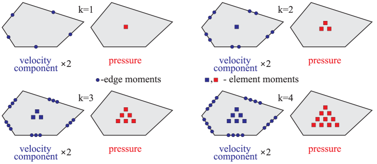
Fig. 1: Illustration of the degrees of freedom for the velocity and pressure solving the two-dimensional Stokes problem.

This choice of degrees of freedom ensures that the discrete differential operators

$$\Pi^{E}_{k-1}\circ\nabla\quad\textrm{and}\quad\Pi^{E}_{k-1}\circ\operatorname{div},$$ (17)

when applied to a vector field $\mathbf{v}_{h}$ in ${\mathbf{V}}_{h}^{k}(E)$ are computable using only the degrees of freedom of $\mathbf{v}_{h}$ on $E$. The projection $\Pi^{E}_{k-1}\nabla\mathbf{v}_{h}$ is defined as

$$(\Pi^{E}_{k-1}(\nabla\mathbf{v}_{h}),\mathbf{m}_{\alpha})_{E}=(\nabla\mathbf{v}_{h},\mathbf{m}_{\alpha})_{E}\qquad\forall\mathbf{m}_{\alpha}\in\big{[}\mathcal{M}_{k-1}(E)\big{]}^{d}.$$

Integration by parts yields:

$$(\nabla\mathbf{v}_{h},\mathbf{m}_{\alpha})_{E}=-(\mathbf{v}_{h},\nabla\mathbf{m}_{\alpha})_{E}+\sum_{s\in\partial E}(\mathbf{n}_{s}\cdot\mathbf{v}_{h},\mathbf{m}_{\alpha})_{s}.$$

Likewise, the projection $\Pi^{E}_{k-1}(\operatorname{div}\mathbf{v}_{h})$ is defined as

$$(\Pi^{E}_{k-1}(\operatorname{div}\mathbf{v}_{h}),m_{\alpha})_{E}=(\operatorname{div}\mathbf{v}_{h},m_{\alpha})_{E}\qquad\forall m_{\alpha}\in\mathcal{M}_{k-1}(E).$$

Integration by parts yields:

$$(\operatorname{div}\mathbf{v}_{h},m_{\alpha})_{E}=-(\mathbf{v}_{h},\nabla m_{\alpha})_{E}+\sum_{s\in\partial E}(\mathbf{n}_{s}\cdot\mathbf{v}_{h},m_{\alpha})_{s}.$$

The components of $\mathbf{m}_{\alpha}\in\big{[}\mathcal{M}_{k-1}(E)\big{]}^{d}$ and $m_{\alpha}\in\mathcal{M}_{k-1}(E)$ are polynomials of degree at most $k-2$ in $E$ and, when restricted to each $s\in\partial E$, are polynomials of degree at most $k-1$. Therefore, the right-hand side of the last equation above is computable using only the internal and the edge/face degrees of freedom of the (scalar) components $\mathbf{v}_{h}$.

Finally, in the virtual element formulation (7)-(8), we use the virtual element space ${\mathbf{V}}_{h,g}^{k}$, whose definition requires the boundary function $\mathbf{g}_{h}$. This function is such that ${\mathbf{g}_{h}}_{|s}$ on every edge/face $s\in\Gamma$ is the $L^{2}$-orthogonal projection of $\mathbf{g}$ on the polynomial space $\mathbb{P}_{k-1}(s)$.

3.5 Approximation of the bilinear forms $a(\cdot,\cdot)$ and $b(\cdot,\cdot)$

In view of the following analysis, it is useful to extend the definition of the continuous bilinear forms $a$ and $b$, to the whole of $H^{1}(\mathcal{T}_{h})$ as a sum of the elemental contributions $a^{E}$ and $b^{E}$,

$$a(\mathbf{u},\mathbf{v})=\sum_{E\in\mathcal{T}_{h}}a^{E}(\mathbf{u},\mathbf{v})\quad\textrm{and}\quad b(\mathbf{u},q)=\sum_{E\in\mathcal{T}_{h}}b^{E}(\mathbf{u},q)\qquad\forall\mathbf{u},\mathbf{v}\in H^{1}(\mathcal{T}_{h}),\,q\in L^{2}(\mathbb{R}),$$

where $a^{E}$ and $b^{E}$ are defined by restricting the integrals in (6) to $E$.

We define the approximate bilinear forms $a_{h}$ and $b_{h}$ used in (7)-(8) by splitting them into local contributions

$$a_{h}(\mathbf{u}_{h},\mathbf{v}_{h}):=\sum_{E\in\mathcal{T}_{h}}a_{h}^{E}(\mathbf{u}_{h},\mathbf{v}_{h})\quad\textrm{and}\quad b_{h}(\mathbf{u}_{h},q_{h}):=\sum_{E\in\mathcal{T}_{h}}b_{h}^{E}(\mathbf{u}_{h},q_{h}),$$

for any $\mathbf{u}_{h},\mathbf{v}_{h}\in{\mathbf{V}}_{h}^{k}$ and $q_{h}\in\Phi_{h}^{k-1}$, where $a_{h}^{E}$ and $b_{h}^{E}$ are bilinear forms on ${\mathbf{V}}_{h}^{k}(E)\times{\mathbf{V}}_{h}^{k}(E)$ and ${\mathbf{V}}_{h}^{k}(E)\times\mathbb{P}_{k-1}(E)$, respectively.

The former bilinear form is defined by:

$$a_{h}^{E}(\mathbf{u}_{h},\mathbf{v}_{h}):=\int_{E}\Pi^{E}_{k-1}(\nabla\mathbf{u}_{h}):\Pi^{E}_{k-1}(\nabla\mathbf{v}_{h})\,d\mathbf{x}+S_{h}^{E}\left(\,(I-\Pi^{\nabla}_{k})\mathbf{u}_{h},(I-\Pi^{\nabla}_{k})\mathbf{v}_{h}\,\right),$$ (18)

where $\Pi^{\nabla}_{k}$ represents the Ritz-Galerkin projection operator introduced in Section 3.3 applied component-wisely. The term $S_{h}^{E}$ is the VEM stabilization term, cf. [7]. This can be any symmetric and coercive bilinear form satisfying

$$c_{*}a(\mathbf{v}_{h},\mathbf{v}_{h})\leq S_{h}^{E}(\mathbf{v}_{h},\mathbf{v}_{h})\leq c^{*}a(\mathbf{v}_{h},\mathbf{v}_{h})\qquad\text{for all}\quad\mathbf{v}_{h}\in{\mathbf{V}}_{h}^{k}(E)\backslash{\big{[}\mathbb{P}_{k}(E)]^{d}},$$ (19)

for two positive constants $c_{*}$ and $c^{*}$ independent of $h$ and the mesh element $E$.

Following [7, 5], in all computations presented in Section 6 we used the choice

$$S_{h}^{E}\left(\,(I-\Pi^{\nabla}_{k})\mathbf{u}_{h},(I-\Pi^{\nabla}_{k})\mathbf{v}_{h}\,\right)=\sum_{i=1}^{N_{E}}\bm{\chi}_{i}\left((I-\Pi^{\nabla}_{k})\mathbf{u}_{h}\right)\cdot\bm{\chi}_{i}\left((I-\Pi^{\nabla}_{k})\mathbf{v}_{h}\right),$$ (20)

where $\bm{\chi}_{i}$ is the vector-valued linear operator that associates any virtual function $\bm{\phi}$ with the vector of its $i$-th local degrees of freedom $\bm{\chi}_{i}(\bm{\phi})\in\mathbb{R}^{d}$.

Remark 2.

Again following [7, 5], we may have defined the consistency term on the right-hand side of (18) as $\int_{E}\nabla\Pi^{\nabla}_{k}\mathbf{u}_{h}:\nabla\Pi^{\nabla}_{k}\mathbf{v}_{h}\,d\mathbf{x}$, but the approach used in (18) is more suitable to generalisations to problems with non-constant coefficients, see, e.g., [23]. Furthermore, the availability of the projection $\Pi^{E}_{k-1}(\nabla\mathbf{v}_{h})$ for all $\mathbf{v}_{h}\in{\mathbf{V}}_{h}^{k}$ proven in the previous section is of its own interest.     

The second bilinear form is defined by:

$$b_{h}^{E}(\mathbf{v}_{h},q_{h}):=\int_{E}q_{h}\Pi^{E}_{k-1}(\operatorname{div}\mathbf{v}_{h})\,d\mathbf{x}.$$ (21)

Remark 3.

We note that $b_{h}^{E}(\cdot,q_{h})=b^{E}(\cdot,q_{h})$ in $H^{1,\text{nc}}_{k}(\mathcal{T}_{h})$ for any $q_{h}\in\Phi_{h}^{k-1}$.     

Definition (18) with the VEM stabilisation term satisfying (19) guarantees that the following polynomial consistency and stability properties are satisfied by the bilinear form $a_{h}^{E}$.

Lemma 1 (Consistency and Stability).

1. Polynomial consistency: If $\mathbf{u}_{h}$ or $\mathbf{v}_{h}$, or both, belong to $\big{[}\mathbb{P}_{k}(E)\big{]}^{d}$, the bilinear form $a_{h}^{E}$ satisfies

   $$a_{h}^{E}(\mathbf{u}_{h},\mathbf{v}_{h})=a^{E}(\mathbf{u}_{h},\mathbf{v}_{h}).$$ (22)

2. Stability: There exist two positive constants $\alpha_{*}$ and $\alpha^{*}$ independent of $h$ and the mesh element $E$ such that, for all $\mathbf{v}_{h}\in{\mathbf{V}}_{h}^{k}(E)$, the bilinear form $a_{h}^{E}$ satisfies

   $$\alpha_{*}a^{E}(\mathbf{v}_{h},\mathbf{v}_{h})\leq a_{h}^{E}(\mathbf{v}_{h},\mathbf{v}_{h})\leq\alpha^{*}a^{E}(\mathbf{v}_{h},\mathbf{v}_{h}).$$ (23)

Proof.  Property $(i)$ is a straightforward consequence of the fact that the stabilization term is zero on polynomial vectors. To prove Property $(ii)$ we first show that $a_{h}^{E}(\mathbf{v}_{h},\mathbf{v}_{h})=0$ implies that $\mathbf{v}_{h}$ is a constant vector, i.e., $a^{E}$ and $a_{h}^{E}$ have the same kernel. Indeed, consider $\mathbf{v}_{h}\in\big{[}V_{h}^{k}(E)\big{]}^{d}$ such that $a_{h}^{E}(\mathbf{v}_{h},\mathbf{v}_{h})=0$. We find that

$$(a)\,\,\int_{E}{\left\lvert\Pi^{E}_{k-1}(\nabla\mathbf{v}_{h})\right\rvert}^{2}\,d\mathbf{x}=0\quad\textrm{and}\quad(b)\,\,S_{h}^{E}\big{(}\,(I-\Pi^{E}_{k})\mathbf{v}_{h},(I-\Pi^{E}_{k})\mathbf{v}_{h}\,\big{)}=0.$$

The coercivity of $S_{h}^{E}$ and property $(b)$ imply that ${\mathbf{v}_{h}}_{|E}=\Pi^{E}_{k}(\mathbf{v}_{h})$, i.e., ${\mathbf{v}_{h}}_{|E}\in\big{[}\mathbb{P}_{k}(E)\big{]}^{d}$, and, thus, ${\nabla\mathbf{v}_{h}}_{|E}=\Pi^{E}_{k-1}(\nabla\mathbf{v}_{h})\in\big{[}\mathbb{P}_{k-1}(E)\big{]}^{d\times d}$. Property $(a)$ implies that $\Pi^{E}_{k-1}(\nabla\mathbf{v}_{h})=0$. Therefore, it holds that ${\nabla\mathbf{v}_{h}}_{|E}=0$; hence, ${\mathbf{v}_{h}}_{|E}$ is a constant vector. Now, (23) follows from (19) as in the scalar case, see [23] for details.     

Remark 4.

As is usual in the virtual element methodology, in order to satisfy conditions (22) and (23), the bilinear form $a_{h}^{E}(\mathbf{u}_{h},\mathbf{v}_{h})$ is built as the sum of a “consistency” and a “stabilising” term, corresponding to the first and the second term in the right-hand side of (18), respectively. The consistency term is exactly computable using only the degrees of freedom of $\mathbf{u}_{h}$ and $\mathbf{v}_{h}$ and satisfies the consistency condition (22). However, the consistency term alone does not satisfy the stability condition (23) on the whole virtual element space due to a rank deficiency of the operator, or equivalently, to the existence of a spurious kernel. Hence, a stabilization term must be added to fix this issue and actually remove the spurious kernel. This latter term is designed to vanish on the polynomial subspace not to affect the consistency property. As such, choice of the stabilization term is not unique [23]. For example, for the closely related MFD method, a number of studies investigated the optimal choice of the stabilization term with respect to a given criterion (reduction of dispersion effects, existence of a discrete maximum/minimum principle), cf. [31, 30, 17]. By exploiting the strict relation existing between the MFD method and the VEM, these alternative constructions of the stabilization term could be optionally considered in the present context.     

3.6 Mesh-dependent energy norms

Hereafter, we shall use the energy semi-norm on the broken Sobolev space $\big{[}H^{1}(\mathcal{T}_{h})\big{]}^{d}$:

$${\left\lvert\mathbf{v}\right\rvert}_{1,h}^{2}:=\sum_{E\in\mathcal{T}_{h}}{\left\lvert\mathbf{v}\right\rvert}_{1,E}^{2}\quad\textrm{with}\quad{\left\lvert\mathbf{v}\right\rvert}_{1,E}^{2}=a^{E}(\mathbf{v},\mathbf{v}).$$

A standard application of the results in [18] shows that a Poincaré inequality holds for the functions in $H_{k}^{1,\text{nc}}(\mathcal{T}_{h})$, $k\geq 1$. Therefore, the semi-norm ${\left\lvert\cdot\right\rvert}_{1,h}$ is a norm in $\big{[}H_{k}^{1,\text{nc}}(\mathcal{T}_{h})\big{]}^{d}$, and for this reason throughout the paper we prefer to use the notation ${\left\lVert\mathbf{v}\right\rVert}_{1,h}$ and ${\left\lVert\mathbf{v}\right\rVert}_{1,E}$ instead of ${\left\lvert\mathbf{v}\right\rvert}_{1,h}$ and ${\left\lvert\mathbf{v}\right\rvert}_{1,E}$. To prove the inf-sup stability, we use the mesh-dependent energy seminorm on ${\mathbf{V}}_{h}^{k}$ given by

$$|||\mathbf{v}_{h}|||^{2}:=\sum_{E\in\mathcal{T}_{h}}|||\mathbf{v}_{h}|||_{E}^{2},$$ (24)

with

$$|||\mathbf{v}_{h}|||_{E}^{2}:=a_{h}^{E}(\mathbf{v}_{h},\mathbf{v}_{h})=\int_{E}{\left\lvert\Pi^{E}_{k-1}(\nabla\mathbf{v}_{h})\right\rvert}^{2}\,d\mathbf{x}+S_{h}^{E}\left(\,(I-\Pi^{E}_{k})\mathbf{v}_{h},(I-\Pi^{E}_{k})\mathbf{v}_{h}\,\right).$$ (25)

Also, we will consider the affine subspace of vector-valued functions ${\mathbf{V}}_{h,g}^{k}=\big{[}V_{h,g}^{k}\big{]}^{d}$ where $V_{h,g}^{k}$ contains the scalar functions of $V_{h}^{k}$ whose trace on the boundary $\Gamma$ is equal to $g$, i.e.,

$$V_{h,g}^{k}:=\Big{\{}v_{h}\in V_{h}^{k}\,|\,{v_{h}}_{|s}=g\textrm{~{}for~{}}s\subset\Gamma\Big{\}},$$ (26)

and the linear subspace $V_{h,0}^{k}$ obtained for $g=0$. On $V_{h,0}^{k}$ we have the following equivalence of norms.

Lemma 2.

The seminorm $|||\,\cdot\,|||$ defined by (24)-(25) is a norm on ${\mathbf{V}}_{h,0}^{k}$ and

$$\sqrt{\alpha_{*}}{\left\lVert\mathbf{v}_{h}\right\rVert}_{1,h}\leq|||\mathbf{v}_{h}|||\leq\sqrt{\alpha^{*}}{\left\lVert\mathbf{v}_{h}\right\rVert}_{1,h}\qquad\forall\mathbf{v}_{h}\in{\mathbf{V}}_{h,0}^{k}.$$ (27)

Proof.  As noted in the proof of the stability condition (23), $|||\mathbf{v}_{h}|||_{E}=0$ implies that ${\mathbf{v}_{h}}_{|E}$ is a constant vector, and, from the definition of $H^{1,\text{nc}}_{k}(\mathcal{T}_{h})$, it follows that $\mathbf{v}_{h}=$ constant. Finally, from $\mathbf{v}_{h}\in{\mathbf{V}}_{h,0}^{k}$ it follows that $\mathbf{v}_{h}=0$. The equivalence between the two norms in (27) is a straightforward consequence of (23).     

3.7 Approximation of the right-hand side $(\mathbf{f},\cdot)$

We approximate the right-hand side term $(\mathbf{f},\,\cdot\,)$ by the linear functional

$$(\mathbf{f}_{h},\mathbf{v}_{h}):=\sum_{E\in\mathcal{T}_{h}}(\mathbf{f}_{h},\mathbf{v}_{h})_{E}\quad\textrm{with}\quad{\mathbf{f}_{h}}_{|E}:=\Pi^{E}_{\max(k-2,0)}(\mathbf{f}).$$ (28)

Since $\Pi^{E}_{\max(k-2,0)}(\mathbf{f})$ is a polynomial of degree at most $k-2$, each local linear functional is bounded and, for $k\geq 2$, it is computable by using the internal degrees of freedom of $\mathbf{v}_{h}$. However, it is not computable for $k=1$. Indeed, the computation of $(\mathbf{f}_{h},\mathbf{v}_{h})_{E}$ above requires the knowledge of the average value of the components of $\mathbf{v}_{h}$ on each element $E$ and such information is only available for $k\geq 2$. Therefore, the case $k=1$ deserves a special treatment. We follow Reference [5] and approximate $\Pi^{E}_{0}(\mathbf{v}_{h})$ by the average of the $0$-th order moments of $\mathbf{v}_{h}$ associated with the edge/face of cell $E$. Namely we consider

$$\overline{\mathbf{v}}_{h}|_{E}=\frac{1}{\nu_{E}}\sum_{s\in\partial E}\frac{1}{|s|}\int_{s}\mathbf{v}_{h}ds,$$

and note that $\overline{\mathbf{v}}_{h}|_{E}$ is a first-order approximation to $\Pi^{E}_{0}(\mathbf{v}_{h})=\frac{1}{|E|}\displaystyle\int_{E}\mathbf{v}_{h}d\mathbf{x}$, i.e., we have that

$${\left\lVert\overline{\mathbf{v}}_{h}|_{E}-\Pi^{E}_{0}(\mathbf{v}_{h})\right\rVert}_{0,E}\leq Ch|\mathbf{v}|_{1,E}.$$

Then, we use $\overline{\mathbf{v}}_{h}$ to compute $(\mathbf{f}_{h},\mathbf{v}_{h})$ through the approximation:

$$\big{(}\Pi^{E}_{0}(\mathbf{f}),\mathbf{v}_{h}\big{)}_{E}=\big{(}\Pi^{E}_{0}(\mathbf{f}),\Pi^{E}_{0}(\mathbf{v}_{h})\big{)}_{E}\approx\big{(}\Pi^{E}_{0}(\mathbf{f}),\overline{\mathbf{v}}_{h}\big{)}_{E}.$$

Therefore, for $k=1$ we take:

$$(\mathbf{f}_{h},\mathbf{v}_{h}):=\sum_{E\in\mathcal{T}_{h}}(\Pi^{E}_{0}(\mathbf{f}),\overline{\mathbf{v}}_{h})_{E}.$$

We collect the results for the approximation of the right-hand side functional $(\mathbf{f},\cdot)$ for $k=1$ and $k>1$ in the following lemma. The proof follows from a straightforward extension of the scalar case, which is found in [5], to $d$-sized vector-valued forcing terms $\mathbf{f}$ and for this reason is omitted.

Lemma 3 (Approximation of the right-hand side $(\mathbf{f},\cdot)$).

Let $m,k\geq 1$ be integer numbers and consider $\mathbf{f}\in\big{[}H^{m-1}(\Omega)\big{]}^{d}$, $r=\min(k,m)$, and $(\mathbf{f}_{h},\cdot)\in\big{[}(V_{h}^{k})^{\prime}\big{]}^{d}$ defined as above. There exists a constant $C$ independent of $h$ such that

$$\sup_{\mathbf{v}_{h}\in{\mathbf{V}}_{h}^{k}}\frac{{\left\lvert(\mathbf{f}_{h},\mathbf{v}_{h})-(\mathbf{f},\mathbf{v}_{h})\right\rvert}}{{\left\lVert\mathbf{v}_{h}\right\rVert}_{1,h}}\leq Ch^{r}{\left\lVert\mathbf{f}\right\rVert}_{r-1}.$$

Proof.  See [5].     

4 Error analysis

The well-posedness of the discrete problem (7)-(8) is discussed in Section 4.1. The non-conformity error is estimated in Section 4.2. The convergence analysis is carried out in Sections 4.3 and 4.4, where error estimates for the approximation of the velocity and pressure fields are respectively derived. For the convergence analysis, we assume that $\mathbf{g}=0$ on $\Gamma$ in (3) through the whole section.

Define the virtual interpolant of the vector field $\mathbf{v}\in\big{[}H^{1,\text{nc}}_{k}(\mathcal{T}_{h})\big{]}^{d}$ as the unique vector field $\mathbf{v}^{\mathtt{I}}\in{\mathbf{V}}_{h}^{k}$ whose degrees of freedom are the internal and edge/face moments of $\mathbf{v}$. Formally,

• for $k\geq 1$, the degrees of freedom of $\mathbf{v}^{\mathtt{I}}$ associated with the edge/face $s\in\mathcal{E}_{h}$ are given by

  $$\mu_{s}^{\alpha}(\mathbf{v}^{\mathtt{I}}):=\int_{s}\mathbf{v}\,m_{\alpha}\,ds,\qquad m_{\alpha}\in\mathcal{M}_{k-1}(s);$$ (29)

• for $k\geq 2$, the degrees of freedom of $\mathbf{v}^{\mathtt{I}}$ associated with the mesh element $E$ are given by

  $$\mu_{E}^{\alpha}(\mathbf{v}^{\mathtt{I}}):=\int_{E}\mathbf{v}\,m_{\alpha}\,d\mathbf{x},\qquad m_{\alpha}\in\mathcal{M}_{k-2}(E).$$ (30)

The above relations must be interpreted component-wise. The unisolvence of the degrees of freedom implies the uniqueness of $\mathbf{v}^{\mathtt{I}}$. Moreover, if $\mathbf{v}\in\big{[}H^{1}_{0}(\Omega)\big{]}^{d}$ all its moments on each edge/face $s$ on $\Gamma$ are zero and, consequently, $\mathbf{v}^{\mathtt{I}}$ belongs to ${\mathbf{V}}_{h,0}^{k}$. We also have the following result regarding the approximation of sufficiently smooth functions by the virtual interpolant, which may be proven as in [5].

Theorem 2 (Approximation using virtual element functions).

Let ${\mathbf{V}}_{h}^{k}$ the non-conforming virtual element space of Section 3.4 for any integer $k\geq 1$, $m$ a positive integer such that $2\leq m\leq k+1$, and $D$ a closed subset of $\Omega$. Under Assumption 1 (mesh regularity), for any $\mathbf{v}\in H^{m}(D)$, there exists an element $\mathbf{v}^{\mathtt{I}}\in{\mathbf{V}}_{h}^{k}$ such that

$${\left\lVert\mathbf{v}-\mathbf{v}^{\mathtt{I}}\right\rVert}_{0,D}+h{\left\lvert\mathbf{v}-\mathbf{v}^{\mathtt{I}}\right\rvert}_{1,D}\leq Ch^{m}{\left\lvert\mathbf{v}\right\rvert}_{m,D},$$

where $C$ is a positive constant that depends only on the polynomial degree $k$ and the mesh regularity constant $\rho$.

4.1 Existence and uniqueness of the virtual element solution

The main result of this section is the existence and uniqueness of the virtual element solution $(\mathbf{u}_{h},p_{h})\in{\mathbf{V}}_{h}^{k}\times\Phi_{h}^{k-1}$, which is stated in Theorem 3. The proof of this theorem is based on the inf-sup property that is proven in the following lemma by adapting a classical argument.

Lemma 4 (Inf-sup).

There exists a strictly positive constant $\beta$ independent of $h$ such that for every $q_{h}$ in $\Phi_{h}^{k-1}$ there exists a vector $\mathbf{v}_{q}$ in ${\mathbf{V}}_{h,0}^{k}$ such that

$$\frac{b_{h}(\mathbf{v}_{q},q_{h})}{|||\mathbf{v}_{q}|||}\geq\beta{\left\lVert q_{h}\right\rVert}_{0}.$$

Proof.  From [16] we know that there exists a strictly positive constant $\widetilde{\beta}$ independent of $h$ such that for every $q$ in $L^{2}(\Omega)/{\mathbb{R}}$ there exists a vector $\hat{\mathbf{v}}_{q}$ in $\big{[}H^{1}_{0}(\Omega)\big{]}^{d}$ such that

$$\frac{b(\hat{\mathbf{v}}_{q},q)}{{\left\lVert\hat{\mathbf{v}}_{q}\right\rVert}_{1}}\geq\widetilde{\beta}{\left\lVert q\right\rVert}_{0}.$$

We can restrict this inequality to $\Phi_{h}^{k-1}\subset L^{2}(\Omega)/{\mathbb{R}}$ and for any $q_{h}\in\Phi_{h}^{k-1}$ consider the corresponding vector $\hat{\mathbf{v}}_{q}$. We will prove that

$$(i)\quad b_{h}(\hat{\mathbf{v}}_{q}^{\mathtt{I}},q_{h})=b(\hat{\mathbf{v}}_{q},q_{h})\quad\forall q_{h}\in\Phi_{h}^{k-1}\quad\textrm{and}\quad(ii)\quad|||\hat{\mathbf{v}}_{q}^{\mathtt{I}}|||\leq\gamma{\left\lVert\hat{\mathbf{v}}_{q}\right\rVert}_{1},$$

where $\hat{\mathbf{v}}_{q}^{\mathtt{I}}$ is the virtual interpolation of $\hat{\mathbf{v}}_{q}$ defined in the previous section and $\gamma=\alpha^{*}/{\sqrt{\alpha_{*}}}$. Such properties easily imply that

$$\frac{b_{h}(\hat{\mathbf{v}}_{q}^{\mathtt{I}},q_{h})}{|||\hat{\mathbf{v}}_{q}^{\mathtt{I}}|||}\geq\frac{b(\hat{\mathbf{v}}_{q},q_{h})}{\gamma{\left\lVert\hat{\mathbf{v}}_{q}\right\rVert}_{1}}\qquad\forall q_{h}\in\Phi_{h}^{k-1},$$

from which the assertion of the lemma follows with $\mathbf{v}_{q}=\hat{\mathbf{v}}_{q}^{\mathtt{I}}$ and $\beta=\widetilde{\beta}/{\gamma}$.

To prove $(i)$, consider the following development that starts from the definition of $b_{h}^{E}$:

$$\begin{array}[]{rll}b_{h}^{E}(\hat{\mathbf{v}}_{q}^{\mathtt{I}},q_{h})&\displaystyle=\int_{E}q_{h}\,\Pi^{E}_{k-1}(\operatorname{div}\hat{\mathbf{v}}_{q}^{\mathtt{I}})d\mathbf{x}&\quad\mbox{[use the definition of $\Pi^{E}_{k-1}$]}\\[7.5pt] &\displaystyle=\int_{E}q_{h}\,\operatorname{div}\hat{\mathbf{v}}_{q}^{\mathtt{I}}d\mathbf{x}&\quad\mbox{[integrate by parts]}\\[7.5pt] &\displaystyle=-\int_{E}\nabla q_{h}\cdot\hat{\mathbf{v}}_{q}^{\mathtt{I}}d\mathbf{x}+\sum_{s\in\partial E}\int_{s}q_{h}\mathbf{n}_{s}\cdot\hat{\mathbf{v}}_{q}^{\mathtt{I}}ds&\quad\mbox{[use the definition of $\hat{\mathbf{v}}_{q}^{\mathtt{I}}$]}\\[7.5pt] &\displaystyle=-\int_{E}\nabla q_{h}\cdot\hat{\mathbf{v}}_{q}d\mathbf{x}+\sum_{s\in\partial E}\int_{s}q_{h}\mathbf{n}_{s}\cdot\hat{\mathbf{v}}_{q}ds&\quad\mbox{[integrate by parts back]}\\[7.5pt] &\displaystyle=\int_{E}q_{h}\,\operatorname{div}\hat{\mathbf{v}}_{q}d\mathbf{x}&\quad\mbox{[use the definition of $b^{E}(\cdot,\cdot)$]}\\[7.5pt] &\displaystyle=b^{E}(\hat{\mathbf{v}}_{q},q_{h})\end{array}$$

Property $(i)$ readily follows from the elemental decomposition of $b_{h}$ and $b$.

To prove $(ii)$, first note that the stability condition of $a_{h}^{E}$ implies that

$$\alpha_{*}{\left\lVert\hat{\mathbf{v}}_{q}^{\mathtt{I}}\right\rVert}_{1,E}^{2}\leq|||\hat{\mathbf{v}}_{q}^{\mathtt{I}}|||_{E}^{2}\leq\alpha^{*}{\left\lVert\hat{\mathbf{v}}_{q}^{\mathtt{I}}\right\rVert}_{1,E}^{2}.$$ (31)

Now, since $\hat{\mathbf{v}}_{q}^{\mathtt{I}}\in V_{h}^{k}(E)$ it holds that $\Delta\hat{\mathbf{v}}_{q}^{\mathtt{I}}$ is a vector of polynomials of degree $k-2$ inside $E$ and $(\mathbf{n}_{s}\cdot\nabla)\hat{\mathbf{v}}_{q}^{\mathtt{I}}$ is a vector of polynomials of degree $k-1$ along each edge $s\in\partial E$ and we have that:

$$\begin{array}[]{rll}a^{E}(\hat{\mathbf{v}}_{q}^{\mathtt{I}},\hat{\mathbf{v}}_{q}^{\mathtt{I}})&\displaystyle=\int_{E}\nabla\hat{\mathbf{v}}_{q}^{\mathtt{I}}:\nabla\hat{\mathbf{v}}_{q}^{\mathtt{I}}\,d\mathbf{x}&\quad\mbox{[integrate by parts]}\\[5.0pt] &\displaystyle=-\int_{E}\hat{\mathbf{v}}_{q}^{\mathtt{I}}\cdot\Delta\hat{\mathbf{v}}_{q}^{\mathtt{I}}\,d\mathbf{x}+\sum_{s\in\partial E}\int_{s}\hat{\mathbf{v}}_{q}^{\mathtt{I}}\cdot(\mathbf{n}_{s}\cdot\nabla)\hat{\mathbf{v}}_{q}^{\mathtt{I}}\,ds&\quad\mbox{[use the definition of $\hat{\mathbf{v}}_{q}^{\mathtt{I}}$]}\\[5.0pt] &\displaystyle=-\int_{E}\hat{\mathbf{v}}_{q}\cdot\Delta\hat{\mathbf{v}}_{q}^{\mathtt{I}}\,d\mathbf{x}+\sum_{s\in\partial E}\int_{s}\hat{\mathbf{v}}_{q}\cdot(\mathbf{n}_{s}\cdot\nabla)\hat{\mathbf{v}}_{q}^{\mathtt{I}}\,ds&\quad\mbox{[integrate by parts back]}\\[5.0pt] &\displaystyle=\int_{E}\nabla\hat{\mathbf{v}}_{q}:\nabla\hat{\mathbf{v}}_{q}^{\mathtt{I}}\,d\mathbf{x}&\quad\mbox{[use the Cauchy-Schwarz inequality]}\\[5.0pt] &\leq\big{(}a^{E}(\hat{\mathbf{v}}_{q},\hat{\mathbf{v}}_{q})\big{)}^{\frac{1}{2}}\big{(}a^{E}(\hat{\mathbf{v}}_{q}^{\mathtt{I}},\hat{\mathbf{v}}_{q}^{\mathtt{I}})\big{)}^{\frac{1}{2}}&\quad\mbox{[use the left inequality of~{}\eqref{eq:stab-vtqI}]}\\[5.0pt] &\leq{\left\lVert\hat{\mathbf{v}}_{q}\right\rVert}_{1,E}\,\frac{1}{\sqrt{\alpha_{*}}}|||\hat{\mathbf{v}}_{q}^{\mathtt{I}}|||_{E}.\end{array}$$

Since ${\left\lVert\hat{\mathbf{v}}_{q}^{\mathtt{I}}\right\rVert}_{1,E}^{2}=a^{E}(\hat{\mathbf{v}}_{q}^{\mathtt{I}},\hat{\mathbf{v}}_{q}^{\mathtt{I}})$, the last inequality and (31) implies that $|||\hat{\mathbf{v}}_{q}^{\mathtt{I}}|||_{E}\leq\alpha^{*}/{\sqrt{\alpha_{*}}}{\left\lVert\hat{\mathbf{v}}_{q}\right\rVert}_{1,E}$ and property $(ii)$ follows from the continuity of $\hat{\mathbf{v}}_{q}$ in $\big{[}H^{1}_{0}(\Omega)\big{]}^{d}$ by summing over all $E\in\mathcal{T}_{h}$ and setting $\gamma=\alpha^{*}/{\sqrt{\alpha_{*}}}$.     

Theorem 3.

The solution of the discrete problem (7)-(8) exists and is unique.

Proof.  Remark 3 implies that $\textsf{ker}(b_{h})=\textsf{ker}(b)$ in $\big{[}H^{1,\text{nc}}_{k}(\mathcal{T}_{h})\big{]}^{d}\times\Phi_{h}^{k-1}$, where

$$\textsf{ker}(b_{h})=\big{\{}\mathbf{v}_{h}\in\big{[}H^{1,\text{nc}}_{k}(\mathcal{T}_{h})\big{]}^{d}\,|\,b_{h}(\mathbf{v}_{h},q_{h})=0\,\,\forall q_{h}\in\Phi_{h}^{k-1}\big{\}}.$$

In view of the stability condition (23), the coercivity of $a_{h}(\cdot,\cdot)$ on $\textsf{ker}(b_{h})$ follows from the coercivity of $a(\cdot,\cdot)$ on $\textsf{ker}(b)$. Therefore, existence and uniqueness of the solution follow from the inf-sup property proved in Lemma 4, cf. [16].     

4.2 Estimate of the non-conformity error

The non-conformity error is controlled as in Lemma 6. The proof of this lemma requires a bound on the jumps of $\mathbf{v}_{h}$ and $\mathbf{n}\mathbf{v}_{h}$ (which, we recall, are defined in (9) and (10)). This bound is provided by Lemma 5.

Lemma 5.

Let $k,m\geq 1$, $r=\min(k,m)$ be integer numbers. Consider $\mathbf{u}\in\big{[}H^{m+1}(\Omega)\big{]}^{d}$ and $p\in L^{2}(\Omega)/{\mathbb{R}}\cap H^{m}(\Omega)$. Then, under Assumption 1 (mesh regularity), for every $\mathbf{v}_{h}\in{\mathbf{V}}_{h,0}^{k}$ it holds

$${\left\lvert\sum_{s\in\mathcal{E}_{h}}\int_{s}\nabla\mathbf{u}:\widetilde{{\left[\!\left[\mathbf{v}_{h}\right]\!\right]}}ds\,\right\rvert}+{\left\lvert\sum_{s\in\mathcal{E}_{h}}\int_{s}p{\left[\!\left[\mathbf{v}_{h}\right]\!\right]}ds\,\right\rvert}\leq Ch^{r}\big{(}{\left\lVert u\right\rVert}_{r+1}+{\left\lVert p\right\rVert}_{r}\big{)}\,{\left\lVert\mathbf{v}_{h}\right\rVert}_{1}.$$

Proof.  Since $\mathbf{v}_{h}\in{\mathbf{V}}_{h}^{k}\subset\big{[}H^{1,\text{nc}}_{k}(\mathcal{T}_{h})\big{]}^{d}$, the jump of the components of $\mathbf{v}_{h}$ on every interface $s$ is orthogonal to the polynomial functions of degree $k-1$ defined along $s$. Thus, it holds that

$$\sum_{s\in\mathcal{E}_{h}}\int_{s}p{\left[\!\left[\mathbf{v}_{h}\right]\!\right]}\,ds=\sum_{s\in\mathcal{E}_{h}}\int_{s}\big{(}p-\Pi^{s}_{k-1}(p)\big{)}\,\big{(}{\left[\!\left[\mathbf{v}_{h}\right]\!\right]}-\Pi^{s}_{k-1}{\left[\!\left[\mathbf{v}_{h}\right]\!\right]}\big{)}ds,$$

for the pressure and

$$\sum_{s\in\mathcal{E}_{h}}\int_{s}\nabla\mathbf{u}:\widetilde{{\left[\!\left[\mathbf{v}_{h}\right]\!\right]}}ds=\sum_{s\in\mathcal{E}_{h}}\int_{s}\big{(}\nabla\mathbf{u}-\Pi^{s}_{k-1}(\nabla\mathbf{u})\big{)}:\big{(}\widetilde{{\left[\!\left[\mathbf{v}_{h}\right]\!\right]}}-\Pi^{s}_{0}\widetilde{{\left[\!\left[\mathbf{v}_{h}\right]\!\right]}}\big{)}ds,$$

for the velocity. Using the Cauchy-Schwartz inequality and then applying component-wise the approximation estimates of Theorem 1 to bound each of the resulting terms, we obtain, cf. [5] or [27],

$${\left\lvert\sum_{s\in\mathcal{E}_{h}}\int_{s}\nabla\mathbf{u}:\widetilde{{\left[\!\left[\mathbf{v}_{h}\right]\!\right]}}ds\,\right\rvert}+{\left\lvert\sum_{s\in\mathcal{E}_{h}}\int_{s}p{\left[\!\left[\mathbf{v}_{h}\right]\!\right]}ds\,\right\rvert}\leq Ch^{r}\sum_{s\in\mathcal{E}_{h}}\Big{(}{\left\lVert\mathbf{u}\right\rVert}_{r+1,E^{+}\cup E^{-}}+{\left\lVert p\right\rVert}_{r,E^{+}\cup E^{-}}\Big{)}{\left\lvert\mathbf{v}_{h}\right\rvert}_{1,E^{+}\cup E^{-}},$$

where for each side $s$ the symbols $E^{+}$ and $E^{-}$ denote the two elements sharing that side. As the number of edges/faces is assumed to be uniformly bounded, the required result follows with a positive constant $C$ independent of $h$ and $\mathbf{u}$.     

Lemma 6 (non-conformity error).

Let $k,m\geq 1$, $r=\min(k,m)$ be integer numbers. Let $\mathbf{u}\in\big{[}H^{1}_{0}(\Omega)\cap H^{m+1}(\Omega)\big{]}^{d}$ and $p\in L^{2}(\Omega)/{\mathbb{R}}\cap H^{m}(\Omega)$ be the velocity and pressure solution of problem (4)-(5), with source term $\mathbf{f}\in\big{[}L^{2}(\Omega)\big{]}^{d}$ and homogeneous boundary condition $\mathbf{g}=0$ on $\Gamma$. Then, for every $\mathbf{v}_{h}\in{\mathbf{V}}_{h,0}^{k}$, it holds that

$${\left\lvert a(\mathbf{u},\mathbf{v}_{h})-(\mathbf{f},\mathbf{v}_{h})\right\rvert}\leq Ch^{r}\Big{(}{\left\lVert\mathbf{u}\right\rVert}_{r+1}+{\left\lVert p\right\rVert}_{r}\Big{)}\,{\left\lVert\mathbf{v}_{h}\right\rVert}_{1}+{\left\lvert b(\mathbf{v}_{h},p)\right\rvert}.$$

Proof.  Test (1) against $\mathbf{v}_{h}\in{\mathbf{V}}_{h,0}^{k}$. For $m\geq 1$ we have at least $\mathbf{u}\in\big{[}H^{2}(\Omega)\big{]}^{2}$ and $p\in H^{1}(\Omega)$ and we can apply the Green’s identity. By rearranging the summation on the internal sides and using the definition of the jump operators given in section 3.1, we obtain:

$$a(\mathbf{u},\mathbf{v}_{h})-(\mathbf{f},\mathbf{v}_{h})=a(\mathbf{u},\mathbf{v}_{h})-(-\Delta\mathbf{u}+\nabla p,\mathbf{v}_{h})=b(\mathbf{v}_{h},p)+\sum_{s\in\mathcal{E}_{h}}\int_{s}\left(\nabla\mathbf{u}:\widetilde{{\left[\!\left[\mathbf{v}_{h}\right]\!\right]}}+p{\left[\!\left[\mathbf{v}_{h}\right]\!\right]}\right)\,ds.$$ (32)

The assertion of the lemma follows by applying the result of Lemma 5.     

4.3 Error estimate for the velocity

Let

$$\mathbf{W}:=\Big{\{}\,\mathbf{w}\in\big{[}H^{1}_{0}(\Omega)\big{]}^{d}\,|\,\operatorname{div}\mathbf{w}=0\,\Big{\}}\quad\textrm{and}\quad\mathbf{W}_{h}^{k}:=\Big{\{}\,\mathbf{w}_{h}\in{\mathbf{V}}_{h,0}^{k}\,|\,\Pi^{E}_{k-1}\circ\operatorname{div}\mathbf{w}_{h}=0\,\Big{\}}.$$ (33)

Using these definitions, problem (4)-(5) is equivalent to [27]:

$$\mbox{\emph{Find $\mathbf{u}\in\mathbf{W}$ such that~{}~{}}}a(\mathbf{u},\mathbf{v})=(\mathbf{f},\mathbf{v})\quad\forall\mathbf{v}\in\mathbf{W},$$ (34)

and problem (7)-(8) is equivalent to [27]:

$$\mbox{\emph{Find $\mathbf{u}_{h}\in\mathbf{W}_{h}^{k}$ such that~{}~{}}}a_{h}(\mathbf{u}_{h},\mathbf{v}_{h})=(\mathbf{f}_{h},\mathbf{v}_{h})\quad\forall\mathbf{v}_{h}\in\mathbf{W}_{h}^{k}.$$ (35)

Theorem 4 ($H^{1}$ abstract a priori error bound for the velocity).

Let $\mathbf{u}\in\mathbf{W}$ be the solution of problem (34), and $\mathbf{u}_{h}\in\mathbf{W}_{h}^{k}$ the solution of problem (35) with $k\geq 1$. Then, it holds that:

$${\left\lVert\mathbf{u}-\mathbf{u}_{h}\right\rVert}_{1,h}\leq \frac{1}{\alpha_{*}}\Bigg{[}\,(1+\alpha^{*})\inf_{\mathbf{v}_{h}\in\mathbf{W}_{h}^{k}}{\left\lVert\mathbf{u}-\mathbf{v}_{h}\right\rVert}_{1,h}+(1+\alpha^{*})\inf_{\mathbf{q}\in[\Phi^{k}_{h}]^{d}}{\left\lVert\mathbf{u}-\mathbf{q}\right\rVert}_{1,h}$$

$$\quad\qquad+\sup_{\begin{subarray}{c}\mathbf{w}_{h}\in\mathbf{W}_{h}^{k}\\ \mathbf{w}_{h}\neq 0\end{subarray}}\frac{{\left\lvert(\mathbf{f}_{h},\mathbf{w}_{h})-(\mathbf{f},\mathbf{w}_{h})\right\rvert}}{{\left\lVert\mathbf{w}_{h}\right\rVert}_{1,h}}\,+\sup_{\begin{subarray}{c}\mathbf{w}_{h}\in\mathbf{W}_{h}^{k}\\ \mathbf{w}_{h}\neq 0\end{subarray}}\frac{{\left\lvert a(\mathbf{u},\mathbf{w}_{h})-(\mathbf{f},\mathbf{w}_{h})\right\rvert}}{{\left\lVert\mathbf{w}_{h}\right\rVert}_{1,h}}\,\Bigg{]}.$$ (36)

The last term in the right-hand side of the above error estimate measures the non-conformity error, i.e. it is non-zero because $\mathbf{W}_{h}^{k}$ is a non-conforming space.

Proof.  Let $\mathbf{v}_{h}$ be an arbitrary element of $\mathbf{W}_{h}^{k}$ and let $\mathbf{w}_{h}=\mathbf{u}_{h}-\mathbf{v}_{h}$. From the stability property of the virtual bilinear form (23) and equation (35) it follows that

$$\alpha_{*}{\left\lVert\mathbf{u}_{h}-\mathbf{v}_{h}\right\rVert}_{1,h}^{2}\leq a_{h}(\mathbf{u}_{h}-\mathbf{v}_{h},\mathbf{w}_{h})=(\mathbf{f}_{h},\mathbf{w}_{h})-a_{h}(\mathbf{v}_{h},\mathbf{w}_{h}).$$

Then, we add and subtract $(\mathbf{f},\mathbf{w}_{h})$ and $a(\mathbf{u},\mathbf{w}_{h})$ and we obtain:

$$\alpha_{*}{\left\lVert\mathbf{u}_{h}-\mathbf{v}_{h}\right\rVert}_{1,h}^{2}\leq\Big{[}(\mathbf{f}_{h},\mathbf{w}_{h})-(\mathbf{f},\mathbf{w}_{h})\Big{]}+\Big{[}(\mathbf{f},\mathbf{w}_{h})-a(\mathbf{u},\mathbf{w}_{h})\Big{]}+\Big{[}a(\mathbf{u},\mathbf{w}_{h})-a_{h}(\mathbf{v}_{h},\mathbf{w}_{h})\Big{]}.$$ (37)

The first term on the right-hand side characterizes the approximation of the source term $\mathbf{f}$ by $\mathbf{f}_{h}$; the second term is the conformity error determined by choosing the test function $\mathbf{w}_{h}$ in $\mathbf{W}_{h}^{k}$ instead of $\mathbf{W}$; the third term simultaneously characterizes the approximation of $\mathbf{u}$ by $\mathbf{v}_{h}$ and $a(\cdot,\cdot)$ by $a_{h}(\cdot,\cdot)$ in $\mathbf{W}_{h}^{k}$. To separate this linked dependence, we reformulate the last term as the summation of local contributions; then, we add and subtract $a^{E}(\mathbf{q},\mathbf{w}_{h})$ and $a_{h}^{E}(\mathbf{q},\mathbf{w}_{h})$ to each summation argument, where $\mathbf{q}$ is a generic vector-valued function in $\big{[}\Phi^{k}_{h}\big{]}^{d}$, and we obtain:

$$a(\mathbf{u},\mathbf{w}_{h})-a_{h}(\mathbf{v}_{h},\mathbf{w}_{h}) =\sum_{E\in\mathcal{T}_{h}}\Big{[}a^{E}(\mathbf{u},\mathbf{w}_{h})-a_{h}^{E}(\mathbf{v}_{h},\mathbf{w}_{h})\Big{]}$$

$$=\sum_{E\in\mathcal{T}_{h}}\Big{[}a^{E}(\mathbf{u}-\mathbf{q},\mathbf{w}_{h})+\big{(}a^{E}(\mathbf{q},\mathbf{w}_{h})-a_{h}^{E}(\mathbf{q},\mathbf{w}_{h})\big{)}+a_{h}^{E}(\mathbf{q}-\mathbf{v}_{h},\mathbf{w}_{h})\Big{]}.$$

Since $\mathbf{q}_{|E}$ is a polynomial vector of degree $k$, the intermediate term above is zero due to the polynomial consistency relation (22). Furthermore, we transform the last term above by using the continuity and stability of the virtual bilinear form:

$$a_{h}^{E}(\mathbf{q}-\mathbf{v}_{h},\mathbf{w}_{h}) \leq\left(a_{h}^{E}(\mathbf{q}-\mathbf{v}_{h},\mathbf{q}-\mathbf{v}_{h})\right)^{\frac{1}{2}}\left(a_{h}^{E}(\mathbf{w}_{h},\mathbf{w}_{h})\right)^{\frac{1}{2}}\leq\alpha^{*}\left(a^{E}(\mathbf{q}-\mathbf{v}_{h},\mathbf{q}-\mathbf{v}_{h})\right)^{\frac{1}{2}}\left(a^{E}(\mathbf{w}_{h},\mathbf{w}_{h})\right)^{\frac{1}{2}}$$

$$=\alpha^{*}{\left\lVert\mathbf{q}-\mathbf{v}_{h}\right\rVert}_{1,E}{\left\lVert\mathbf{w}_{h}\right\rVert}_{1,E}.$$

Hence, for all $\mathbf{v}_{h},\mathbf{w}_{h}\in\mathbf{W}_{h}^{k}$ with $\mathbf{w}_{h}\neq\mathbf{0}$ and $\mathbf{q}\in\big{[}\Phi_{h}^{k}\big{]}^{d}$, using the last inequality and the continuity of $a^{E}(\cdot,\cdot)$, multiplying and dividing by ${\left\lVert\mathbf{w}_{h}\right\rVert}_{1,h}$, and using the triangle inequality ${\left\lVert\mathbf{q}-\mathbf{v}_{h}\right\rVert}_{1,h}\leq{\left\lVert\mathbf{q}-\mathbf{u}\right\rVert}_{1,h}+{\left\lVert\mathbf{u}-\mathbf{v}_{h}\right\rVert}_{1,h}$, we find that

$$\alpha_{*}{\left\lVert\mathbf{u}_{h}-\mathbf{v}_{h}\right\rVert}_{1,h}\leq\frac{{\left\lvert(\mathbf{f}_{h},\mathbf{w}_{h})-(\mathbf{f},\mathbf{w}_{h})\right\rvert}}{{\left\lVert\mathbf{w}_{h}\right\rVert}_{1,h}}+\frac{{\left\lvert(\mathbf{f},\mathbf{w}_{h})-a(\mathbf{u},\mathbf{w}_{h})\right\rvert}}{{\left\lVert\mathbf{w}_{h}\right\rVert}_{1,h}}+\alpha^{*}{\left\lVert\mathbf{u}-\mathbf{v}_{h}\right\rVert}_{1,h}+\big{(}1+\alpha^{*}\big{)}{\left\lVert\mathbf{u}-\mathbf{q}\right\rVert}_{1,h}.$$

The result now follows by applying the estimates above to the triangle inequality

$${\left\lVert\mathbf{u}-\mathbf{u}_{h}\right\rVert}_{1,h}\leq{\left\lVert\mathbf{u}-\mathbf{v}_{h}\right\rVert}_{1,h}+{\left\lVert\mathbf{v}_{h}-\mathbf{u}_{h}\right\rVert}_{1,h},$$

properly taking the supremum upper bound of the terms with $\mathbf{w}_{h}$ and the infimum over the arbitrary vector functions $\mathbf{q}$ and $\mathbf{v}_{h}$.     

Theorem 5 ($H^{1}$ error bound for the velocity).

Let $k,m\geq 1$, $r=\min(k,m)$ be integer numbers. Assuming that $\mathbf{f}\in\big{[}H^{m-1}(\Omega)\big{]}^{d}$, let $\mathbf{u}\in\big{[}H^{1}_{0}(\Omega)\cap H^{m+1}(\Omega)\big{]}^{d}$ and $p\in L^{2}(\Omega)/{\mathbb{R}}\cap H^{m}(\Omega)$ be the exact velocity and pressure solution to problem (4)-(5) (with $\mathbf{g}=0$ on $\Gamma$). Let $(\mathbf{f}_{h},\mathbf{v}_{h}):=\sum_{E\in\mathcal{T}_{h}}(\mathbf{f}_{h},\mathbf{v}_{h})_{E}$, with ${\mathbf{f}_{h}}_{|E}$ defined as in section 3.7. Denote by $\mathbf{u}_{h}\in\mathbf{W}_{h}^{k}$ the virtual element solution to problem (35) under Assumption 1 (mesh regularity), where $\mathbf{W}_{h}^{k}$ is the divergence-free non-conforming virtual element space of vector-valued functions defined in (33). Then, there exists a constant $C$ independent of $h$ such that

$${\left\lVert\mathbf{u}-\mathbf{u}_{h}\right\rVert}_{1,h}\leq Ch^{r}({\left\lVert\mathbf{u}\right\rVert}_{r+1}+{\left\lVert p\right\rVert}_{r}+{\left\lVert\mathbf{f}\right\rVert}_{r-1}).$$

Proof.  Since $\mathbf{u}$ is also solution of problem (34), we start the proof of the theorem by separately bounding the terms of the abstract bound of Theorem 4. The first term on the right-hand side of (36), i.e. $\inf_{\mathbf{v}_{h}\in\mathbf{W}_{h}^{k}}{\left\lVert\mathbf{u}-\mathbf{v}_{h}\right\rVert}_{1,h}$, is easily bounded by introducing the virtual interpolant $\mathbf{u}^{\mathtt{I}}\in{\mathbf{V}}_{h}^{k}$ of $\mathbf{u}$ as in Theorem 2 and noting that $\mathbf{u}^{\mathtt{I}}$ belongs to $\mathbf{W}_{h}^{k}$. Indeed, for any element $E$, we have $\Pi^{E}_{k-1}(\operatorname{div}\mathbf{u}^{\mathtt{I}})\in\mathbb{P}_{k-1}(E)$ and for any polynomial $q\in\mathbb{P}_{k-1}(E)$ we have that:

$$\int_{E}q\Pi^{E}_{k-1}(\operatorname{div}\mathbf{u}^{\mathtt{I}})\,d\mathbf{x} =\int_{E}q\operatorname{div}\mathbf{u}^{\mathtt{I}}d\mathbf{x}=-\int_{E}\nabla q\cdot\mathbf{u}^{\mathtt{I}}d\mathbf{x}+\sum_{s\in\partial E}\int_{s}q\mathbf{n}_{s}\cdot\mathbf{u}^{\mathtt{I}}ds$$

$$=-\int_{E}\nabla q\cdot\mathbf{u}d\mathbf{x}+\sum_{s\in\partial E}\int_{s}q\mathbf{n}_{s}\cdot\mathbf{u}ds=\int_{E}q\operatorname{div}\mathbf{u}\,d\mathbf{x}=0.$$

Hence, $\Pi^{E}_{k-1}(\operatorname{div}\mathbf{u}^{\mathtt{I}})=0$. Likewise, the second term is bounded by using in each cell $E$ the results of Theorem 1 since

$$\inf_{\mathbf{q}\in[\Phi^{k}_{h}]^{d}}{\left\lVert\mathbf{u}-\mathbf{q}\right\rVert}_{1,h}\leq{\left\lVert\mathbf{u}-\Pi^{E}_{k}(\mathbf{u})\right\rVert}_{1,h}.$$

The bound on the third term is given by Lemma 3 since $\mathbf{w}_{h}\in\mathbf{W}_{h}^{k}\subset{\mathbf{V}}_{h}^{k}$. The bound on the fourth term is given by Lemma 6 and noting that $b(\mathbf{w}_{h},p)=0$ for every $\mathbf{w}_{h}\in\mathbf{W}_{h}^{k}$. Finally, the assertion of the theorem follows by combining the bounds derived above and noting that the inequality constant $C$ may depend only on the stability constants $\alpha_{*}$ and $\alpha^{*}$, and the mesh regularity constant $\rho$.     

Remark 5.

Optimal order error estimates for the velocity approximation in the $L^{2}$-norm can be derived by duality arguments, see always [27]. However, a more accurate approximation of the forcing terms than that provided by (28) would be needed for the case $k=1,2$. This can be obtained by following the approach in [8].

4.4 Error estimate for the pressure

Let $p^{\mathtt{I}}$ denote the piecewise polynomial function that is defined on each elements $E$ of mesh $\mathcal{T}_{h}$ by the orthogonal projection of $p$ on the space of polynomials of degree $k-1$; formally, $(p^{\mathtt{I}})_{|E}=\Pi^{E}_{k-1}(p)\in\mathbb{P}_{k-1}(E)$. The accuracy of this approximation is characterized by Theorem 1. To ease the notation we will also use the symbol $p^{\mathtt{I}}_{E}$ to denote the restriction $(p^{\mathtt{I}})_{|E}$.

Theorem 6 (Abstract $L^{2}$ a priori error bound for the pressure).

Let $k\geq 1$ be an integer number. Let $\mathbf{u}\in\big{[}H^{1}_{0}(\Omega)\cap H^{2}(\Omega)\big{]}^{d}$ and $p\in L^{2}(\Omega)/{\mathbb{R}}\cap H^{1}(\Omega)$ be the exact velocity and pressure solution to problem (4)-(5) with the homogeneous boundary condition $\mathbf{g}=0$ on $\Gamma$. Denote the projection of $p$ in $\Phi_{h}^{k-1}$ by $p^{\mathtt{I}}$. Let $(\mathbf{f}_{h},\mathbf{v}_{h}):=\sum_{E\in\mathcal{T}_{h}}(\mathbf{f}_{h},\mathbf{v}_{h})_{E}$, with ${\mathbf{f}_{h}}_{|E}$ defined as in section 3.7. Let $\mathbf{u}_{h}\in{\mathbf{V}}_{h,0}^{k}$ and $p_{h}\in\Phi_{h}^{k-1}$ be the virtual element velocity and pressure solution to problem (7)-(8) under Assumption 1. Then, it holds that

$${\left\lVert p_{h}-p^{\mathtt{I}}\right\rVert}_{0}\leq\frac{\alpha^{*}}{\sqrt{\alpha_{*}}\beta}\left(\,\alpha^{*}{\left\lVert\mathbf{u}-\mathbf{u}_{h}\right\rVert}_{1,h}+(1+\alpha^{*})\inf_{\mathbf{q}\in[\Phi^{k}_{h}]^{d}}{\left\lVert\mathbf{u}-\mathbf{q}\right\rVert}_{1,h}\phantom{\sup_{\begin{subarray}{c}\mathbf{v}_{h}\in{\mathbf{V}}_{h,0}^{k}\\ \mathbf{v}_{h}\neq 0\end{subarray}}\frac{{\Big{\lvert}\sum_{s\in\mathcal{E}_{h}}\int_{s}p{\left[\!\left[\mathbf{v}_{h}\right]\!\right]}ds\Big{\rvert}}}{{\left\lVert\mathbf{v}_{h}\right\rVert}_{1,h}}}\right.$$

$$\quad+\left.\sup_{\begin{subarray}{c}\mathbf{v}_{h}\in{\mathbf{V}}_{h,0}^{k}\\ \mathbf{v}_{h}\neq 0\end{subarray}}\frac{\displaystyle{\big{\lvert}(\mathbf{f}_{h},\mathbf{v}_{h})-(\mathbf{f},\mathbf{v}_{h})\big{\rvert}}+{\big{\lvert}b(\mathbf{v}_{h},p-p^{\mathtt{I}})\big{\rvert}}+{\Big{\lvert}\sum_{s\in\mathcal{E}_{h}}\int_{s}\nabla\mathbf{u}:\widetilde{{\left[\!\left[\mathbf{v}_{h}\right]\!\right]}}ds\Big{\rvert}}+{\Big{\lvert}\sum_{s\in\mathcal{E}_{h}}\int_{s}p{\left[\!\left[\mathbf{v}_{h}\right]\!\right]}ds\Big{\rvert}}}{{\left\lVert\mathbf{v}_{h}\right\rVert}_{1,h}}\right).$$ (38)

Proof.  Take $q=p_{h}-p^{\mathtt{I}}\in\Phi_{h}^{k-1}$. From Lemma 4, we know that there exists a vector $\mathbf{v}_{h}$ such that $\beta{\left\lVert p_{h}-p^{\mathtt{I}}\right\rVert}_{0}\,|||\mathbf{v}_{h}|||\leq b_{h}(\mathbf{v}_{h},p_{h}-p^{\mathtt{I}})$, and, in view of the norm equivalence (27), it holds that

$$\beta{\left\lVert p_{h}-p^{\mathtt{I}}\right\rVert}_{0}\leq\frac{b_{h}(\mathbf{v}_{h},p_{h}-p^{\mathtt{I}})}{\sqrt{\alpha_{*}}{\left\lVert\mathbf{v}_{h}\right\rVert}_{1,h}}\leq\sup_{\begin{subarray}{c}\mathbf{v}_{h}\in{\mathbf{V}}_{h,0}^{k}\\ \mathbf{v}_{h}\neq 0\end{subarray}}\frac{b_{h}(\mathbf{v}_{h},p_{h}-p^{\mathtt{I}})}{\sqrt{\alpha_{*}}{\left\lVert\mathbf{v}_{h}\right\rVert}_{1,h}}.$$ (39)

We use (7), and add and subtract $(\mathbf{f},\mathbf{v}_{h})$ and $a(\mathbf{u},\mathbf{v}_{h})$ to obtain:

$$b_{h}(\mathbf{v}_{h},p_{h}-p^{\mathtt{I}}) =(\mathbf{f}_{h},\mathbf{v}_{h})-a_{h}(\mathbf{u}_{h},\mathbf{v}_{h})-b_{h}(\mathbf{v}_{h},p^{\mathtt{I}})$$

$$=\Big{[}(\mathbf{f}_{h},\mathbf{v}_{h})-(\mathbf{f},\mathbf{v}_{h})\Big{]}+\Big{[}(\mathbf{f},\mathbf{v}_{h})-a(\mathbf{u},\mathbf{v}_{h})\Big{]}+\Big{[}a(\mathbf{u},\mathbf{v}_{h})-a_{h}(\mathbf{u}_{h},\mathbf{v}_{h})\Big{]}-b_{h}(\mathbf{v}_{h},p^{\mathtt{I}}).$$ (40)

We test (1) against $\mathbf{v}_{h}\in{\mathbf{V}}_{h,0}^{k}$, apply the Green’s identity, rearrange the summation on edges/faces in $\mathcal{E}$, and introduce the jump notation (cf. section 3.1) to obtain:

$$(\mathbf{f},\mathbf{v}_{h})-a(\mathbf{u},\mathbf{v}_{h})=(-\Delta\mathbf{u}+\nabla p,\mathbf{v}_{h})-a(\mathbf{u},\mathbf{v}_{h})$$

$$\qquad=b(\mathbf{v}_{h},p)-\left(\sum_{E\in\mathcal{T}_{h}}\int_{\partial E}(\mathbf{n}\cdot\nabla)\mathbf{u}\cdot\mathbf{v}_{h}ds-\sum_{E\in\mathcal{T}_{h}}\int_{\partial E}p\mathbf{n}\cdot\mathbf{v}_{h}ds\right)$$

$$\qquad=b(\mathbf{v}_{h},p)-\sum_{s\in\mathcal{E}_{h}}\int_{s}\Big{(}(\mathbf{n}_{s}^{+}\cdot\nabla)\mathbf{u}\cdot\mathbf{v}_{h}^{+}+(\mathbf{n}_{s}^{-}\cdot\nabla)\mathbf{u}\cdot\mathbf{v}_{h}^{-}\Big{)}\,ds+\sum_{s\in\mathcal{E}_{h}}\int_{s}p(\mathbf{n}_{s}^{+}\cdot\mathbf{v}_{h}^{+}+\mathbf{n}_{s}^{-}\cdot\mathbf{v}_{h}^{-})\,ds$$

$$\qquad=b(\mathbf{v}_{h},p)-\sum_{s\in\mathcal{E}_{h}}\int_{s}\left(\nabla\mathbf{u}:\widetilde{{\left[\!\left[\mathbf{v}_{h}\right]\!\right]}}-p{\left[\!\left[\mathbf{v}_{h}\right]\!\right]}\right)\,ds.$$ (41)

Also, from Remark 3 we know that $b_{h}(\mathbf{v}_{h},p^{\mathtt{I}})=b(\mathbf{v}_{h},p^{\mathtt{I}})$, and using this relation and (41) in (40) we obtain:

$$b_{h}(\mathbf{v}_{h},p_{h}-p^{\mathtt{I}}) =\Big{[}(\mathbf{f}_{h},\mathbf{v}_{h})-(\mathbf{f},\mathbf{v}_{h})\Big{]}+\Big{[}a(\mathbf{u},\mathbf{v}_{h})-a_{h}(\mathbf{u}_{h},\mathbf{v}_{h})\Big{]}+b(\mathbf{v}_{h},p-p^{\mathtt{I}})$$

$$-\sum_{s\in\mathcal{E}_{h}}\int_{s}\left(\nabla\mathbf{u}:\widetilde{{\left[\!\left[\mathbf{v}_{h}\right]\!\right]}}-p{\left[\!\left[\mathbf{v}_{h}\right]\!\right]}\right)\,ds.$$ (42)

The second term on the right-hand side can be further bounded by introducing a generic vector $\mathbf{q}\in[\Phi^{k}_{h}]^{d}$ and reasoning as in the proof of Theorem 4, thus yielding

$${\big{\lvert}a(\mathbf{u},\mathbf{v}_{h})-a_{h}(\mathbf{u}_{h},\mathbf{v}_{h})\big{\rvert}}\leq\left(\alpha^{*}{\left\lVert\mathbf{u}-\mathbf{u}_{h}\right\rVert}_{1,h}+\big{(}1+\alpha^{*}\big{)}{\left\lVert\mathbf{u}-\mathbf{q}\right\rVert}_{1,h}\right){\left\lVert\mathbf{v}_{h}\right\rVert}_{1,h}.$$ (43)

The assertion of the theorem follows from (39) by taking the absolute value of (42) with (43) ${\left\lVert\mathbf{v}_{h}\right\rVert}_{1,h}$ and the supremum on $\mathbf{v}_{h}$ and $\mathbf{q}$.     

Theorem 7 ($L^{2}$ a priori error bound for the pressure).

Under the assumptions and notations of Theorem 5, let $\mathbf{u}_{h}\in{\mathbf{V}}_{h,0}^{k}$ and $p_{h}\in\Phi_{h}^{k-1}$ be the virtual element velocity and solution to problem (7)-(8). Then, there exists a constant $C>0$ depending only on the stability constants $\alpha_{*}$ and $\alpha^{*}$, the inf-sup constant $\beta$ and the mesh regularity constant $\rho$ such that

$${\left\lVert p-p_{h}\right\rVert}\leq Ch^{r}\big{(}{\left\lVert\mathbf{u}\right\rVert}_{r+1}+{\left\lVert p\right\rVert}_{r}+{\left\lVert\mathbf{f}\right\rVert}_{r-1}\big{)}.$$ (44)

Proof.  The proof is just a matter of bounding the terms of the abstract bound of Theorem 6. Bounds for the first, second, and third term are already given in Theorem 5. The bound for the term containing $b(\mathbf{v}_{h},p-p^{\mathtt{I}})$ follows from the polynomial approximation results of Theorem 1. The last two terms are bounded by using Lemma 5.     

5 Implementation details

According to section 3.4, the key component of the VEM implementation is the construction of the projection operators $\Pi^{E}_{k-1}\circ\nabla$, $\Pi^{E}_{k-1}\circ\operatorname{div}$, and $\Pi^{\nabla}_{k}$. Once these projection operators are constructed, all terms in the local bilinear forms can be computed as integrals of polynomials just as in the standard FEM with the only exception of the stabilization term in $a_{h}^{E}$. This latter term does not require any integration but is directly defined through the action of the projector operator $\Pi^{\nabla}_{k}$ on the degrees of freedom.

The matrix representation of $\Pi^{E}_{k-1}\circ\nabla$ and $\Pi^{E}_{k-1}\circ\operatorname{div}$ can be derived from the corresponding representation of the scalar projection operator $\Pi^{E}_{k-1}\circ\tfrac{\partial}{\partial x_{i}}$, $i=1,\ldots,d$, which has already been worked out in [23]. Similarly, we refer to [2] for the details on the computation of $\Pi^{\nabla}_{k}$. In the rest of this section we show how to compute the two terms of the bilinear form $a_{h}^{E}$, i.e., the consistency and stability term, cf. Remark 4, assuming a matrix representation of the projectors is given. The implementation formulas for the bilinear form $b_{h}^{E}$ and the right-hand side linear functional $(\mathbf{f}_{h},\cdot)_{E}$ can be derived similarly and are not shown here.

Consider the Lagrangian basis $\{\phi_{i}\}$ for the scalar virtual element space $V_{h}^{k}(E)$ associated with the degrees of freedom introduced in Section 3.3. We collect the coefficients of the expansion of each monomials $m_{\alpha}$ on the basis $\big{\{}\phi_{i}\big{\}}$ for $\alpha=1,\ldots,N_{d,k}$ on the columns of matrix $\mathbb{D}$, so that $m_{\alpha}=\sum_{j=1}^{N_{E}}\phi_{j}\mathbb{D}_{j,\alpha}$. Similarly, we collect the coefficients of the expansions of the polynomials $\Pi^{\nabla}_{k}\phi_{i}$ and $\Pi^{E}_{k-1}\big{(}{\partial\phi_{i}}/{\partial x_{i}}\big{)}$ with respect to the monomial basis $\big{\{}m_{\alpha}\big{\}}$ on the columns of matrices $\bm{\Pi}_{k}^{\nabla}$ and $\bm{\Pi}_{k-1}^{E,x^{l}}$, respectively. Hence, these projections can be expressed by the formulas

$$\Pi^{E}_{k-1}\left(\frac{\partial\phi_{i}}{\partial x_{l}}\right) =\sum_{\alpha=1}^{N_{d,k}}m_{\alpha}\big{(}\bm{\Pi}_{k-1}^{E,x^{l}}\big{)}_{\alpha,i}\quad\textrm{and}\quad\Pi^{\nabla}_{k}\phi_{i} =\sum_{\alpha=1}^{N_{d,k}}m_{\alpha}\big{(}\bm{\Pi}_{k}^{\nabla}\big{)}_{\alpha,i}=\sum_{j=1}^{N_{E}}\phi_{j}\big{(}\mathbb{D}\bm{\Pi}_{k}^{\nabla}\big{)}_{j,i},$$ (45)

where $(\star)_{i,j}$ denotes the $i,j$-th element of a given matrix argument $\star$. Then, for the local discrete velocity space ${\mathbf{V}}_{h}^{k}(E)$, we consider the set of basis functions $\{\bm{\phi}_{i}^{l}\}$ that are such that $(\bm{\phi}_{i}^{l})_{l^{\prime}}=\phi_{i}$ if $l^{\prime}=l$ and $(\bm{\phi}_{i}^{l})_{l^{\prime}}=0$ otherwise. The generic entry of the consistency term of $a_{h}^{E}$ in (18) is given by

$$\int_{E}\Pi^{E}_{k-1}(\nabla\bm{\phi}_{i}^{l}):\Pi^{E}_{k-1}(\nabla\bm{\phi}_{j}^{l})\,d\mathbf{x}=\sum_{l^{\prime}=1}^{d}\int_{E}\Pi^{E}_{k-1}\left(\frac{\partial\phi_{i}}{\partial x_{l^{\prime}}}\right)\,\Pi^{E}_{k-1}\left(\frac{\partial\phi_{j}}{\partial x_{l^{\prime}}}\right)\,d\mathbf{x}$$

$$\quad=\sum_{l^{\prime}=1}^{d}\sum_{\alpha,\beta=1}^{N_{d,k-1}}\big{(}\bm{\Pi}_{k-1}^{E,x_{l^{\prime}}}\big{)}_{\alpha,i}\big{(}\bm{\Pi}_{k-1}^{E,x_{l^{\prime}}}\big{)}_{\beta,j}\int_{E}m_{\alpha}\,m_{\beta}\,d\mathbf{x}=\sum_{l^{\prime}=1}^{d}\Big{(}\big{(}\bm{\Pi}_{k-1}^{E,x_{l^{\prime}}}\big{)}^{T}\mathbb{H}\big{(}\bm{\Pi}_{k-1}^{E,x_{l^{\prime}}}\big{)}\big{)}_{i,j},$$ (46)

where $\mathbb{H}$ is the matrix with coefficients $\big{(}\mathbb{H}\big{)}_{\alpha,\beta}=\int_{E}m_{\alpha}\,m_{\beta}\,d\mathbf{x}$ for $\alpha,\beta=1,\ldots,N_{d,k-1}$. These coefficients may be computed exactly in special cases or by applying a sufficiently accurate integration rule in general. Similarly, the generic entry of the stabilisation term of $a_{h}^{E}$, which is defined in (20), is given by

$$S_{h}^{E}\left(\,(I-\Pi^{\nabla}_{k})\bm{\phi}_{i}^{l},(I-\Pi^{\nabla}_{k})\bm{\phi_{j}^{l}}\,\right) =\sum_{r=1}^{N_{E}}\bm{\chi}_{r}\left((I-\Pi^{\nabla}_{k})\phi_{i}\right)\cdot\bm{\chi}_{r}\left((I-\Pi^{\nabla}_{k})\phi_{j}\right)$$

$$=\Big{(}\big{(}\mathbb{I}-\mathbb{D}\bm{\Pi}_{k}^{\nabla}\big{)}^{T}\big{(}\mathbb{I}-\mathbb{D}\bm{\Pi}_{k}^{\nabla}\big{)}\Big{)}_{i,j}$$ (47)

since, trivially, $\bm{\chi}_{r}(I-\Pi^{\nabla}_{k})\phi_{i}=\big{(}\mathbb{I}-\mathbb{D}\bm{\Pi}_{k}^{\nabla}\big{)}_{i,r}$.

6 Numerical Results

The numerical experiments that we present in this section are aimed at confirming the a priori analysis developed in the previous sections. In a preliminary stage, the consistency of non-conforming VEM, i.e. the exactness for polynomial solutions, has been tested numerically by solving the Stokes equation with boundary and source data determined by $\mathbf{u}(x,y)=(y^{m},x^{m})$ and $p=x^{m}+y^{m}$ on different set of polygonal meshes and for $m=1$ to $4$. In all the cases, we measure an error whose magnitude is of the order of the arithmetic precision, thus confirming this property.

To study the accuracy of the method we solve the problem with the following solution on the domain $\Omega=]0,1[\times]0,1[$:

$$\mathbf{u}(x,y)=\left(\begin{array}[]{c}2\pi\,f(x)\sin(2\pi y)\\ f^{\prime}(x)\cos(2\pi y)\end{array}\right),\qquad p(x,y)=\sin(2\pi x)\sin(2\pi y),$$ (50)

with $f(x)=x^{5}\,e^{-x}$. The forcing term and the Dirichlet boundary condition are set in accordance with (50).

The performance of the VEM for $k=1,2,3,4$ is investigated by evaluating the rate of convergence on three different sequences of five meshes, labeled by $\mathcal{M}_{1}$, $\mathcal{M}_{2}$ and $\mathcal{M}_{3}$, respectively. The top panels of Fig. 2 show the first mesh of each sequence and the bottom panels show the mesh of the first refinement.

Fig. 2: First (top) and second (bottom) mesh of the three mesh families $\mathcal{M}_{1}$ (left), $\mathcal{M}_{2}$ (middle) and $\mathcal{M}_{3}$ (right).

The meshes in $\mathcal{M}_{1}$ are built by partitioning the domain $\Omega$ into square cells and relocating each interior node to a random position inside a square box centered at that node. The sides of this square box are aligned with the coordinate axis and their length is equal to $0.8$ times the minimum distance between two adjacent nodes of the initial square mesh. The meshes in $\mathcal{M}_{2}$ are built as follows. First, we determine a primal mesh by remapping the position $(\widehat{x},\widehat{y})$ of the nodes of a uniform square partition of $\Omega$ by the smooth coordinate transformation:

$$x =\widehat{x}+(1/{10})\sin(2\pi\widehat{x})\sin(2\pi\widehat{y}),$$

$$y =\widehat{y}+(1/{10})\sin(2\pi\widehat{x})\sin(2\pi\widehat{y}).$$

The corresponding mesh of $\mathcal{M}_{2}$ is built from the primal mesh by splitting each quadrilateral cell into two triangles and connecting the barycenters of adjacent triangular cells by a straight segment. The mesh construction is completed at the boundary by connecting the barycenters of the triangular cells close to the boundary to the midpoints of the boundary edges and these latters to the boundary vertices of the primal mesh. The meshes in $\mathcal{M}_{3}$ are obtained by filling the unit square with a suitably scaled non-convex octagonal reference cell.

All the meshes are parametrised by the number of partitions in each direction. The starting mesh of every sequence is built from a $5\times 5$ regular grid, and the refined meshes are obtained by doubling this resolution. Mesh data for each refinement level, i.e., numbers of mesh elements, number of edges, number of vertices, are reported in Table 1. More details on these mesh constructions can be found in [14, 11]. The mesh data structures are created and managed using the C++ mesh manager tool described in [15].

	Randomised quadrilaterals				Remapped hexagons				Non-convex octagons
$n$	$\mathcal{N}_{E}$	$\mathcal{N}_{e}$	$\mathcal{N}_{v}$	$h$	$\mathcal{N}_{E}$	$\mathcal{N}_{e}$	$\mathcal{N}_{v}$	$h$	$\mathcal{N}_{E}$	$\mathcal{N}_{e}$	$\mathcal{N}_{v}$	$h$
$1$	​$25$	​$60$	​$36$	$0.331$	​$36$	​$125$	​$90$	$0.328$	​$25$	​$120$	​$96$	$0.291$
$2$	​$100$	​$220$	​$121$	$0.186$	​$121$	​$400$	​$280$	$0.185$	​$100$	​$440$	​$341$	$0.146$
$3$	​$400$	​$840$	​$441$	$0.094$	​$441$	​$1400$	​$960$	$0.097$	​$400$	​$1680$	​$1281$	$0.073$
$4$	​$1600$	​$3280$	​$1681$	$0.047$	​$1681$	​$5200$	​$3520$	$0.049$	​$1600$	​$6560$	​$4961$	$0.036$
$5$	​$6400$	​$12960$	​$6561$	$0.024$	​$6561$	​$20000$	​$13440$	$0.025$	​$6400$	​$25920$	​$19521$	$0.018$

Table 1: Mesh data for the meshes in $\mathcal{M}_{1}$, $\mathcal{M}_{2}$, and $\mathcal{M}_{3}$; $\mathcal{N}_{E}$, $\mathcal{N}_{e}$ and $\mathcal{N}_{v}$ are the numbers of mesh elements, interfaces and vertices, respectively, and $h$ is the mesh size parameter.

For the approximation of the velocity, we compare the polynomial quantities $\Pi^{E}_{k}(\mathbf{u}_{h})$ and $\Pi^{E}_{k-1}(\nabla\mathbf{u}_{h})$ with the exact velocity $\mathbf{u}$ and the gradient $\nabla\mathbf{u}$. We recall that we can compute these projections exactly using only the degrees of freedom of the vector and scalar field $\mathbf{u}_{h}$ although we do not know this field. For the approximation of the pressure, we compare the piecewise polynomial fields $p_{h}$ and $\nabla p_{h}$ with the exact pressure $p$ and gradient $\nabla p$.

The relative error curves for pressure and velocity versus the mesh size $h$ are shown respectively in the log-log plots of Figures 3 and 4 for the three mesh sequences as indicated therein. The plots on the left show the relative errors for the approximation of the velocity or pressure field, while the plots on the right show the relative errors for the approximation of the field’s gradient. The expected slopes are shown for each error curve directly on the plots and indicated by numerical labels.

These results are in very good agreement with the convergence rates that are predicted by the analysis of the previous sections.

\begin{overpic}[scale={0.73}]{./pressureL2joint.pdf} \put(75.0,-8.0){{Mesh size $h$}} \put(-12.0,38.0){\begin{sideways}{Pressure $L^{2}$ errors}\end{sideways}} \end{overpic}

\begin{overpic}[scale={0.73}]{./pressureH1joint.pdf} \put(75.0,-8.0){{Mesh size $h$}} \put(-12.0,38.0){\begin{sideways}{Pressure $H^{1}$ errors}\end{sideways}} \end{overpic}

Fig. 3: Relative error curves for the non-conforming VEM approximation of the pressure (left) and its gradient (right) on the three mesh families $\mathcal{M}_{1}$-$\mathcal{M}_{3}$ with $k$ from $1$ to $4$. The expected slopes are indicated by triangles and labels on the plots.

\begin{overpic}[scale={0.73}]{./velocityL2joint.pdf} \put(75.0,-8.0){{Mesh size $h$}} \put(-12.0,38.0){\begin{sideways}{Velocity $L^{2}$ errors}\end{sideways}} \end{overpic}

\begin{overpic}[scale={0.73}]{./velocityH1joint.pdf} \put(75.0,-8.0){{Mesh size $h$}} \put(-12.0,38.0){\begin{sideways}{Velocity $H^{1}$ errors}\end{sideways}} \end{overpic}

Fig. 4: Relative error curves for the non-conforming VEM approximation of the velocity (left) and its gradient (right) on the three mesh families $\mathcal{M}_{1}$-$\mathcal{M}_{3}$ with $k$ from $1$ to $4$. The expected slopes are indicated by triangles and labels on the plots.

7 Conclusions

We presented the non-conforming formulation of the virtual element method for the steady Stokes problem. We have been able to construct approximations of any order in two and three space dimensions in a unified fashion, a feat which is still out of reach for standard non-conforming finite elements. Moreover, the method is naturally defined on general polygonal and polyhedral meshes. In particular non-convex polygons and polyhedra with parallel adjacent interfaces are allowed. The formulation of the method relies on the element-wise construction of virtual approximation spaces for velocity and pressure, which are characterized by a positive integer order $k$. The local approximation space for the velocity contains vectors of polynomials of order $k$ plus other functions that are not computed explicitly and dealt only in terms of their degrees of freedom. The local approximation space for the pressure consists of all polynomials of order $k-1$. We proved that the velocity-pressure pair of global approximation spaces satisfies the inf-sup condition, from which the stability and well-posedness of the scheme follow. We also proved the optimal convergence of the numerical approximation to the velocity and pressure solution fields. The accuracy of the approximation is determined by the degree $k$ of the polynomials and optimal a priori error estimates was derived for the velocity and pressure.

References

- [1] J. Aghili, S. Boyaval, and D. A. Di Pietro. Hybridization of mixed high-order methods on general meshes and application to the Stokes equations, 18 June 2014. Tech. Report. Hal-01009723-v1 (url: https://hal.archives-ouvertes.fr/hal-01009723).
- [2] B. Ahmad, A. Alsaedi, F. Brezzi, L. D. Marini, and A. Russo. Equivalent projectors for virtual element methods. Comput. Math. Appl., 66(3):376–391, 2013.
- [3] M. Ainsworth. Robust a posteriori error estimation for nonconforming finite element approximation. SIAM Journal on Numerical Analysis, 42(6):2320–2341, 2005.
- [4] P. F. Antonietti, L. Beirão da Veiga, D. Mora, and M. Verani. A stream virtual element formulation of the Stokes problem on polygonal meshes. SIAM J. Numer. Anal., 52(1):386–404, 2014.
- [5] B. Ayuso de Dios, K. Lipnikov, and G. Manzini. The nonconforming virtual element method. ESAIM Math. Model. Numer. Anal., (50):879–904, 2016.
- [6] A. E. Baran and G. Stoyan. Gauss-Legendre elements: a stable, higher order non-conforming finite element family. Computing, 79(1):1–21, 2007.
- [7] L. Beirão da Veiga, F. Brezzi, A. Cangiani, G. Manzini, L. D. Marini, and A. Russo. Basic principles of virtual element methods. Math. Models Methods Appl. Sci., 23(1):199–214, 2013.
- [8] L. Beirão da Veiga, F. Brezzi, and L. D. Marini. Virtual elements for linear elasticity problems. SIAM J. Numer. Anal., 51(2):794–812, 2013.
- [9] L. Beirão da Veiga, V. Gyrya, K. Lipnikov, and G. Manzini. Mimetic finite difference method for the Stokes problem on polygonal meshes. J. Comput. Phys., 228(19):7215–7232, 2009.
- [10] L. Beirão da Veiga, K. Lipnikov, and G. Manzini. Error analysis for a mimetic discretization of the steady Stokes problem on polyhedral meshes. SIAM J. Numer. Anal., 48(4):1419–1443, 2010.
- [11] L. Beirão da Veiga, K. Lipnikov, and G. Manzini. Arbitrary-order nodal mimetic discretizations of elliptic problems on polygonal meshes. SIAM J. Numer. Anal., 49(5):1737–1760, 2011.
- [12] L. Beirão da Veiga, K. Lipnikov, and G. Manzini. The mimetic finite difference method for elliptic problems, volume 11 of MS&A. Modeling, Simulation and Applications. Springer, Cham, 2014.
- [13] L. Beirão da Veiga, C. Lovadina, and G. Vacca. Divergence free virtual elements for the Stokes problem on polygonal meshes, 2016. Tech. Report. arXiv:1510.01655. Accepted for publication in ESAIM. Mathematical Modelling and Numerical Analysis. DOI: 10.1051/m2an/2016032.
- [14] L. Beirão da Veiga and G. Manzini. A virtual element method with arbitrary regularity. IMA J. Numer. Anal., 34(2):759–781, 2014.
- [15] E. Bertolazzi and G. Manzini. Algorithm 817: P2MESH: generic object-oriented interface between 2-D unstructured meshes and FEM/FVM-based PDE solvers. ACM Transactions on Mathematical Software (TOMS), 28(1):101–132, 2002.
- [16] D. Boffi, F. Brezzi, and M. Fortin. Mixed finite element methods and applications. Springer series in computational mathematics. Springer, Berlin, Heidelberg, 2013.
- [17] V. A. Bokil, N. L. Gibson, V. Gyrya, and D. A. McGregor. Dispersion reducing methods for edge discretizations of the electric vector wave equation. Journal of Computational Physics, 287:88–109, 2015.
- [18] S. C. Brenner. Poincaré-Friedrichs inequalities for piecewise functions. SIAM J. Numer. Anal., 41(1):306–324, 2003.
- [19] S. C. Brenner and L. R. Scott. The Mathematical Theory of Finite Element Methods. Springer, 2008.
- [20] E. Burman and B. Stamm. Bubble stabilized discontinuous Galerkin method for Stokes’ problem. Math. Models Methods Appl. Sci., 20(02):297–313, 2010.
- [21] E. Cáceres and G. N. Gatica. A mixed virtual element method for the pseudostress-velocity formulation of the Stokes problem. IMA Journal of Numerical Analysis, 2016. Online publication, doi:10.1093/imanum/drw002.
- [22] Z. Cai, J. Douglas, and X. Ye. A stable nonconforming quadrilateral finite element method for the stationary Stokes and Navier–Stokes equations. Calcolo, 36(4):215–232, 1999.
- [23] A. Cangiani, G. Manzini, and O. J. Sutton. Conforming and nonconforming virtual element methods for elliptic problems, June 2016. To appear in IMA Journal of Numerical Analysis.
- [24] B. Cockburn, N. C. Nguyen, and J. Peraire. A comparison of hdg methods for stokes flow. J. Sci. Comput., 45(1–3):215–237, October 2010.
- [25] B. Cockburn and K. Shi. Devising methods for Stokes flow: An overview. Computers & Fluids, 98:221–229, 2014. 12th {USNCCM} mini-symposium of High-Order Methods for Computational Fluid Dynamics - A special issue dedicated to the 80th birthday of Professor Antony Jameson.
- [26] M. Crouzeix and R. S. Falk. Nonconforming finite elements for the Stokes problem. Math. Comp., 52:437–456, 1989.
- [27] M. Crouzeix and P. A. Raviart. Conforming and nonconforming finite element methods for solving the stationary Stokes equations. I. Rev. Francaise Automat. Informat. Recherche Opérationnelle Sér. Rouge, 7(R-3):33–75, 1973.
- [28] T. Dupont and L. R. Scott. Polynomial approximation of functions in Sobolev spaces. Math. Comp., 34(150):441–463, 1980.
- [29] M. Fortin and M. Soulie. A non-conforming piecewise quadratic finite element on triangles. International Journal for Numerical Methods in Engineering, 19(4):505–520, 1983.
- [30] V. Gyrya and K. Lipnikov. M-adaptation method for acoustic wave equation on square meshes. J. Comp. Acoustics, 20(4):1250022:1–23, 2012.
- [31] V. Gyrya, K. Lipnikov, G. Manzini, and D. Svyatskiy. M-adaptation in the mimetic finite difference method. Math. Models Methods Appl. Sci., 24:1621–1663, 2014.
- [32] K. Lipnikov and G. Manzini. A high-order mimetic method on unstructured polyhedral meshes for the diffusion equation. J. Comput. Physics, 272:360–385, 2014.
- [33] K. Lipnikov, G. Manzini, and M. Shashkov. Mimetic finite difference method. J. Comput. Phys., 257(part B):1163–1227, 2014.
- [34] G. Matthies. Inf-sup stable nonconforming finite elements of higher order on quadrilaterals and hexahedra. ESAIM: Mathematical Modelling and Numerical Analysis, 41(5):855–874, 2007.
- [35] G. Matthies and L. Tobiska. Inf-sup stable non-conforming finite elements of arbitrary order on triangles. Numerische Mathematik, 102(2):293–309, 2005.
- [36] R. Rannacher and S. Turek. Simple nonconforming quadrilateral Stokes element. Numerical Methods for Partial Differential Equations, 8(2):97–111, 1992.
- [37] G. Stoyan and A. E. Baran. Crouzeix-Velte decompositions for higher-order finite elements. Comput. Math. Appl., 51(6-7):967–986, 2006.
- [38] J. Wang and X. Ye. A weak Galerkin finite element method for the Stokes equations. Advances in Computational Mathematics, 42(1):155–174, 2016.