Explosive Particle Dispersion in Plasma Turbulence

Abstract

Particle dynamics are investigated in plasma turbulence, using self-consistent kinetic simulations, in two dimensions. In steady state, the trajectories of single protons and proton-pairs are studied, at different values of plasma $\beta$ (ratio between kinetic and magnetic pressure). For single-particle displacements, results are consistent with fluids and magnetic field line dynamics, where particles undergo normal diffusion for very long times, with higher $\beta$’s being more diffusive. In an intermediate time range, with separations lying in the inertial range, particles experience an explosive dispersion in time, consistent with the Richardson prediction. These results, obtained for the first time with a self-consistent kinetic model, are relevant for astrophysical and laboratory plasmas, where turbulence is crucial for heating, mixing and acceleration processes.

The motion of particles in complex fields has been one of the most fascinating problems in physics, with interdisciplinary applications that span from hydrodynamics to astrophysical plasmas. The study of Lagrangian tracers is complementary to the theory of turbulence Kolmogorov (1941) wherein individual tracers undergo a random motion, asymptotically approaching the diffusive Brownian behavior Langevin (1908). The relative motion of a pair of tracers is a different and more subtle problem, as the growth of separation may reflect turbulent correlations Richardson (1926). Both individual and pair particle transport are of great importance in applications ranging from laboratory plasmas Taylor and McNamara (1971); Hauff et al. (2009) to magnetic field wandering and tangling in the galaxy Jokipii and Parker (1969); Eyink et al. (2013); Lazarian et al. (2015), corona Lepreti et al. (2012) and interplanetary medium Ruffolo et al. (2003, 2004). Often discussed in the purely diffusive limit, these varieties of transport may also frequently display nondiffusive (superdiffusive or subdiffusive) behavior (e.g., Perrone et al. (2013)). These subjects have been studied mainly in the test-particle approximation, appropriate, for example, in describing high energy cosmic rays Jokipii (1966).

When the transported particles are elements of the thermal plasma Taylor and McNamara (1971); Balescu et al. (1994), the distribution is often taken as an equilibrium Maxwellian. In this context, test-particles and passive tracers in Magnetohydrodynamics (MHD) have been of interest Dmitruk et al. (2004); Ruffolo et al. (2004); Zimbardo et al. (2006); Busse et al. (2007). However, for low collisonality plasmas where kinetic effects typically generate strong departures from thermal Maxwellian equilibria Marsch (1990), one should treat the transport problem self-consistently. We present first results on this fundamental topic in the present Letter.

In the case of stationary random motion, a single fluid element at position ${\bm{x}}(t)$ and velocity ${\bm{v}(t)}$ has a finite auto-correlation time (or Lagrangian integral time)

$$\tau_{\ell}=\frac{1}{\langle{v(t_{0})}^{2}\rangle}\int_{0}^{\infty}\langle{\bm{v}}(t_{0})\cdot{\bm{v}}(t_{0}+\tau)\rangle d\tau=\frac{D_{s}}{\langle v^{2}\rangle},$$ (1)

where the ensemble $\langle\bullet\rangle$ has been computed over a large number of realizations, positions and times, and $D_{s}$ is the diffusion coefficient. The mean square displacement of $\Delta{\bm{s}}={\bm{x}}(t_{0}+\tau)-{\bm{x}}(t_{0})$, in the limit of $\tau\gg\tau_{\ell}$, obeys

$$\langle\Delta{s}^{2}\rangle=2D_{s}\tau.$$ (2)

The above represents the long-time limit diffusive behavior, typical of Brownian motion. In the opposite limit, $\tau\rightarrow 0$, in the so-called dissipative range, particles conform to ballistic transport, governed by $\langle\Delta{s}^{2}\rangle\sim\tau^{2}$ (Batchelor, 1950; Falkovich et al., 2001).

Together with the asymptotic behavior of single particle motion, it is interesting to consider the motion of two particles, as done by Richardson (1926). In this pioneering work it was predicted that, at intermediate separations, the inner-particle distance $r^{2}\equiv|{\bm{r}}_{1,2}|^{2}=|{\bm{x}}_{1}(\tau)-{\bm{x}}_{2}(\tau)|^{2}$ is super-diffusive in time. Averaging over time and volume, it is observed that

$$\langle r^{2}\rangle\sim\tau^{3}.$$ (3)

This motion is very rapid, explosive in time, and is related to the mixing properties of a turbulent field. Richardson obtained this law from basic principles, computing solutions to the particle-pairs probability distribution, and using hints from observations. Note that this work has been a precursor of Kolmogorov theory of turbulence, and here will be applied to kinetic self-consistent models of plasmas.

Single particle displacement and pair dispersion are here investigated in plasmas, using self-consistent kinetic models of turbulence Servidio et al. (2012); Haynes et al. (2014); Franci et al. (2015). We study the motion of the plasma particles themselves, represented by elements of the proton distribution function, in the phase-space given by position and velocity. We will emphasize a novel study of the particle statistics in a collisionless plasma, in a driven turbulent state, for different plasma parameters.

Driven simulations of the hybrid-PIC model (kinetic ions and fluid electrons) have been performed (ions hereafter are intended to be protons), in a 2.5D geometry, solving (Winske, 1985; Matthews, 1994)

$$\frac{\partial\bm{x}}{\partial t}=\bm{v},~{}~{}\frac{\partial\bm{v}}{\partial t}=\bm{E}+\bm{v}\times\bm{B},$$

$$\frac{\partial\bm{B}}{\partial t}\!=\!-\bm{\nabla}\!\times\!\bm{E}\!=\!\!\bm{\nabla}\!\times\!\!\!\left[\bm{u}\!\times\!\bm{B}\!-\!\frac{1}{\rho}\bm{j}\!\times\!\bm{B}\!+\!\!\frac{1}{\rho}\bm{\nabla}P_{e}\!\!-\!\!\eta\bm{j}\!\right]\!,$$ (4)

where $\bm{x}$ are the proton positions and $\bm{v}$ their velocities, $\bm{B}=\bm{b}+B_{0}{\hat{\bm{z}}}$ is the total (solenoidal) magnetic field, $\bm{j}=\bm{\nabla}\times\bm{B}$ is the current density, $\rho$ and $\bm{u}$ represent the proton (electron) density and the proton bulk velocity, respectively. Electron pressure $P_{e}$ is adiabatic, with $\beta_{e}=\beta_{p}=\beta$, and a small resistivity $\eta$ suppresses small grid-scale activity. Space is normalized to the proton skin depth $d_{p}$, time with the proton cyclotron frequency $\Omega_{cp}$, velocities to the thermal speed $v_{th}$, and magnetic field with Alfvèn speed of the mean magnetic field $B_{0}$. A spatial grid of $N_{x}\times N_{y}=512^{2}$ mesh points is defined in a periodic box of side $L_{0}=128d_{p}$. A large number (1500) of particles-per-cell (ppc) has been chosen to suppress the statistical noise. Three values of plasma $\beta$ (thermal/magnetic pressure) are chosen, as reported in Table 1. The initial fluctuations are chosen with random phases, and with the Fourier modes satisfying $3\leq m\leq 7$, where the $k$-vector is defined as $k=\frac{2\pi}{128d_{p}}m$. Fluctuations have $b_{rms}=v_{rms}=0.5$, with $B_{0}=1$. Proton heating in low-noise simulations is moderate Franci et al. (2015), and the value of the effective $\beta$ at the end of each simulation is increased by $\sim 12\%$.

	$\beta$	$\gamma$	$\tau_{\ell}$	$\tau_{\ell g}$	$D_{s}$	$D_{s}^{(a)}$	$\mu$	$\chi_{0}$
Run I	$0.1$	$1.07$	$11$	$22$	$2.66$	$2.56$	$1.97$	$0.11$
Run II	$0.5$	$1.07$	$5$	$17$	$2.77$	$2.65$	$1.99$	$0.15$
Run III	$5.0$	$1.21$	$1$	$7$	$3.64$	$3.64$	$1.80$	$0.47$

Table 1: Plasma $\beta$; structure function exponent $\gamma$; Lagrangian integral times ($\tau_{\ell}$ and $\tau_{\ell g}$, in units of $\Omega_{cp}^{-1}$); diffusion coefficient $D_{s}$ and its expectation $D_{s}^{(a)}$; pair-dispersion exponent $\mu$ and pair-diffusion coefficient $\chi_{0}$.

To achieve steady state turbulence in a plasma, we borrow ideas from hydrodynamics Chen et al. (1993); Bec et al. (2010); Thalabard et al. (2014). We initially let the system decay freely, and then we introduce a forcing at the peak of nonlinearity $t_{\star}$ (roughly the peak of $\langle j_{z}^{2}\rangle$ Mininni and Pouquet (2009)), with $t_{\star}\sim 25\Omega_{cp}^{-1}$. The forcing consists of “freezing” the amplitude of the large scale modes of the inplane magnetic field, with $1\leq m\leq 4$, leaving the phases unchanged. This corresponds to a large scale input of energy. We perform the analysis described below when a steady state has been achieved, for $50<t\Omega_{cp}<250$.

To characterize turbulence, we computed the second order structure function of the magnetic field $S_{b}({\bm{\delta}})=\langle\left[{\bm{b}}\left({\bm{x}}+{\bm{\delta}},t\right)-{\bm{b}}\left({\bm{x}},t\right)\right]^{2}\rangle_{V,T}$, where $\langle\bullet\rangle_{V,T}$ represents a double average over volume and time. Positions $\bm{x}$ and increments $\bm{\delta}$ are in the $(x,y)$ plane. For an isotropic inertial range of turbulence,

$$S_{b}(\delta)\sim\delta^{\gamma}.$$ (5)

As reported in Fig. 1, the structure function manifests a clear self-similar range. Fitting with Eq. (5), we find that $\gamma$ is quite close to unity, as reported in the Table 1. Note that in classical 3D hydrodynamic turbulence at large Reynolds number, $\gamma=2/3$, corresponding to the celebrated Kolmogorov law Kolmogorov (1941). In plasmas the case is more complex, and it can depend on other factors, such as compressibility, dimensionality and anisotropy, as well as the effective Reynolds numbers. Note, however, that observations and simulations suggest non-universality of plasma turbulence Lee et al. (2010); Tessein et al. (2009).

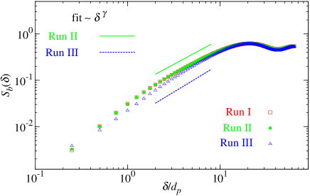
Figure 1: Structure function of the magnetic field as a function of the spatial increment $\delta$, for all the Runs. Full (green) and dashed (blue) lines represent the fit with Eq. (5), for Run II and III, respectively. Exponents $\gamma$ are given in Table 1.

We computed the auto-correlation function $C_{b}({\bm{\delta}})=\langle{\bm{b}}\left({\bm{x}}+{\bm{\delta}},t\right)\cdot{\bm{b}}\left({\bm{x}},t\right)\rangle_{V,T}$, and the auto-correlation length as $\lambda_{C}=\int_{0}^{L_{0}/2}C_{b}(q)dq$. For these simulations $\lambda_{C}\sim 9d_{p}$, which provides a large scale bound to Eq. (5). Analogously, one might identify the small scale termination of the inertial range approximately as the Taylor microscale, which in our case is $\lambda_{T}=\sqrt{\langle b^{2}\rangle/\langle j^{2}\rangle}\sim 1.5d_{p}$. ¿From Fig. 1, Eq. (5) holds for $\lambda_{T}<\delta<\lambda_{C}$. It is interesting to note that, at the highest $\beta$ (Run III), a slightly shorter inertial range is observed, with an higher value of $\gamma$. This is possibly due to an higher damping of the Alfvénic and magnetosonic activity.

We analyzed a subset of $N_{p}$ randomly selected particles, represented by particle-in-cell pseudo-particles, with $N_{p}=10^{5}$. Convergence tests have been performed varying $N_{p}$ from $5\times 10^{4}$ to $N_{p}=2\times 10^{5}$ showing no significant difference. The space-time trajectories of some “puffs” of particles, located at different (randomly selected) regions, are reported in Fig. 2. In the same plot, shaded contours reports $j_{z}$ at $t\Omega_{cp}\sim 50$ and $250$. Particles bunches spread explosively in time, with a very fast departure in the first 10-30 cyclotron times. The inset shows the initial spreading of the central puff, together with some the trajectories of the associated gyro-centers. Gyro-center positions have been computed as ${\bm{x}}_{g}(t)=(1/T)\int_{t-T/2}^{t+T/2}{\bm{x}}(t^{\prime})dt^{\prime}$, using the gyroperiod $T=2\pi{\Omega_{cp}^{-1}}$. The initial separation suggests a superdiffusive behavior, while at very long times the motion seems to be uncorrelated and erratic. Trajectories vary greatly: some remain near the origin; others experience long flights; some rapidly change direction. These differences may reveal interesting correlations between particles and local structures Ruffolo et al. (2003); Tooprakai et al. (2007); Drake et al. (2010); Zank et al. (2015), and will be matter of future investigations. As mentioned above, some trajectories are similar to test particles in MHD or model fields Seripienlert et al. (2010).

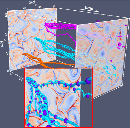
Figure 2: “Puffs” of particles as a function of time, starting from the steady state, located at different regions of 2D plasma turbulence. $j_{z}$ is shown at two times, $t\Omega_{cp}=50,250$ (shaded surfaces). The inset shows the initial spreading of a population (small subset), up to $t\Omega_{cp}\sim 75$ (small spheres), together with the position of some gyrocenters (big spheres). Explosive dispersion is observed.

To understand the ergodic motion in Fig. 2, we analyzed single-particle statistics. We computed the Lagrangian correlation times defined by Eq. (1), for both particles ${\bm{x}}(t)$ and gyro-centers ${\bm{x}}_{g}(t)$. These correlation times $\tau_{\ell}$ and $\tau_{\ell g}$, reported in the Table for all runs, are larger than the cyclotron time and depend on the value of $\beta$, being much smaller for higher $\beta$’s. This faster decorrelation is evidently due to the higher plasma thermal noise which decorrelates the motion earlier. The gyrocenters have longer decorrelation times.

To establish the link between plasma particles and fluid tracers, we analyzed the single-particle displacement $\langle{\Delta s}^{2}\rangle$. Here brackets indicate again an average over particles and times. Following Eq. (2), one can compute the running diffusion coefficient as $D_{s}=\frac{1}{2}\frac{\partial\langle{{\Delta{s}^{2}}}\rangle}{\partial\tau}$. If the displacement is stochastic, for times $\tau\gg\tau_{\ell}$, $D_{s}\rightarrow const.$ On the contrary, for $\tau\rightarrow 0$, $\langle{\Delta s}^{2}\rangle\sim\tau^{2}$, typical of ballistic transport. As reported in Fig. 3, $\langle\Delta s^{2}\rangle$ behaves asymptotically as $\sim\tau$. The horizontal lines indicating $D_{s}$ computed as a fit for very large times, namely $\tau>90\Omega_{cp}^{-1}\gg\tau_{\ell}$. This value can be compared with the asymptotic coefficient, computed from Eq. (1) as $D_{s}^{(a)}=\int_{0}^{\infty}\langle{\bm{v}}(t_{0})\cdot{\bm{v}}(t_{0}+\tau)\rangle d\tau$. As it can be seen, from the figure and the Table, the long-time diffusive limit is evident (Taylor and McNamara, 1971; Okuda and Dawson, 1973). As expected from the Lagrangian correlation times estimation, plasmas with higher $\beta$ (Run III) are more diffusive, with the decorrelation being faster, due to the enhanced importance of fast microscopic particle speeds. (Note that the typical oscillation of running diffusion coefficients, commonly observed in test-particle studies, have a period on the order of the cyclotron time.) In the inset of Fig. 3, the mean square displacement is shown at earlier times, for Run II (all the runs have similar behavior, not shown here). It is evident that the Batchelor regime, where $\sim\tau^{2}$ (Falkovich et al., 2001), is observed for $\tau<1.7\Omega_{cp}^{-1}\ll\tau_{\ell}$.

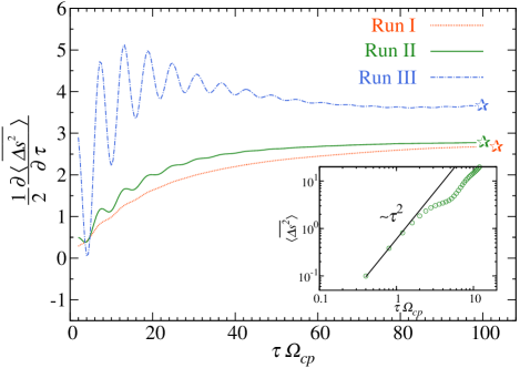
Figure 3: Running diffusion coefficients $\frac{1}{2}\frac{\partial\langle{\Delta s^{2}}\rangle}{\partial\tau}$ for all the runs. Stars indicate $D_{s}$, computed as a fit for very large times $\tau\Omega_{cp}>90$. The inset shows the mean square displacement $\langle\Delta s^{2}\rangle$ in the very initial stage (Run II).

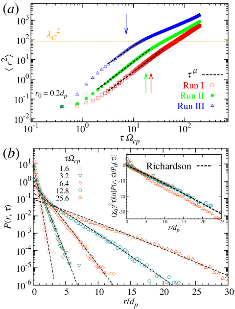
Figure 4: (a) Mean squared gyro-centers separation as a function of time. Inertial range fits $\sim\tau^{\mu}$ are reported (black dashed lines) (see Table I for $\mu$.) The horizontal (orange) dotted line represents $\lambda_{C}$, while arrows indicate $\tau_{\ell g}$. (b) Particle separation probability $P(r,\tau)$ as a function of $r$, at different $\tau$. Results are shown for the intermediate $\beta$ (Run II) but are similar for all the runs. The Richardson fit is reported with dashed (black) lines. Inset of (b): rescaled $P(r,\tau)$ for the same times (symbols) and Richardson expectation ($-r^{\gamma}$) (dashed line). The generalized law is clearly observed for $t\sim\tau_{\ell g}$ , being lost when $t\gg\tau_{\ell g}$ (red triangles).

For times on the order of $\tau_{\ell}$ and $\tau_{\ell g}$, an interesting transient is observed, resembling the super-diffusive behavior typical of fluids. These time ranges correspond to the fast dispersive motion observed in Fig. 2. We study the temporal behavior of gyrocenters distances $r(\tau)$ (in order to avoid the trivial particle gyroperiod), randomly selected in our system, where the initial separation $r_{0}$ has been chosen to be sufficiently small. In ordinary fluids, in order to capture inertial range super-diffusion, this separation must fall in the dissipative length-scales. In our case we chose $r_{0}=0.2d_{p}$, which falls in the secondary (dissipative) range, as it can be observed from Figs. 1-3. Note that results do not depend on this choice for $0.1<r_{0}d_{p}^{-1}<0.5$ (not shown here). In analogy with the single diffusion analysis, we computed the mean squared perpendicular particle pair separation $\langle r^{2}\rangle(\tau)$, reported in Fig. 4-(a). After an initial transient, the mean square separation manifests a self-similar law, with $\langle r^{2}\rangle\sim\tau^{\mu}$. The index slightly depends on the plasma beta, and is between 1.8 and 2 (see Table I).

Fig. 4-(a) also indicates that after the typical separation exceeds the correlation scale $\lambda_{c}$, normal diffusive behavior is established. Analogously, the lower boundary is given by the dispersive-dissipative length, here on the order of the proton skin depth $d_{p}$. The vertical arrows represents the characteristic Lagrangian times $\tau_{\ell g}$, indicating that the diffusive scaling law for plasmas appears on timescales on the order of this decorrelation mechanism. Diffusive asymptotic behavior is observed at very large times. Lower $\beta$’s show a more clear super-diffusive dispersion, while at higher $\beta$ particles are less sensitive to the ${\bf E}\times{\bf B}$ inertial range, which narrows the range of superdiffusion. It is evident that the temporal behavior is “slower” than the hydrodynamic law in Eq. (3), and this apparent difference will be explained as follows.

In analogy with the Richardson work Richardson (1926), and since an exact scaling law for compressible anisotropic Vlasov plasmas has not yet been formulated, we will study $P(r,\tau)$, namely the probability that particles are separated by a distance $r$, at a time $\tau$. Richardson indeed hypothesized that the probability satisfies Richardson (1926); Balkovsky and Lebedev (1998)

$$\frac{\partial P(r,\tau)}{\partial\tau}\!=\!\frac{1}{r}\frac{\partial}{\partial r}\!\left[r\chi(r)\frac{\partial P(r,\tau)}{\partial r}\right],~{}~{}\chi(r)=\chi_{0}r^{2-\gamma}.$$ (6)

Here $\chi(r)$ is a scale-dependent eddy-diffusivity due to turbulence, and in regular fluids, if the Kolmogorov law is observed, $\chi(r)\sim r^{4/3}$. In analogy with his intuition, we infer $\chi(r)$ in Eq. (6) using the exponent in Eq. (5), as suggested by Balkovsky and Lebedev (1998). Given an initial condition $P(r,\tau=0)=\delta(r-r_{0})$, and $\int\!P(r,\tau)rdr\!=\!1$, Eq. (6) admits a general solution Balkovsky and Lebedev (1998):

$$P(r,\tau)=\frac{A}{\left(\chi_{0}\gamma^{2}\tau\right)^{\frac{2}{\gamma}}}e^{-\frac{r^{\gamma}}{\chi_{0}\gamma^{2}\tau}}\equiv P_{0}(\tau)e^{-\frac{r^{\gamma}}{\chi_{0}\gamma^{2}\tau}}.$$ (7)

The above is a solution for $r$ sufficiently larger than $r_{0}$, for separation-times which correspond to inertial range length-scales, and where $\gamma$ is again the exponent of the second order structure function. In Fig. 4-(b), $P(r,\tau)$ is shown, for Run II (all runs have similar results), together with Eq. (7). The latter have been fitted varying $A$, and keeping the same $\chi_{0}$ over for all the inertial range times. As it can be seen, the distribution describes very well the pair dispersion mechanism. In the inset of Fig. 4-(b), the normalized $P(r,\tau)$ are reported, rescaling the distribution in time according to Eq. (7). The generalized law is clearly observed for intermediate times, while is less robust for $\tau\sim 26\Omega_{cp}^{-1}$, where $\langle r^{2}\rangle$ approaches $\lambda_{C}^{2}$ [compare panel (a) and (b)]. Finally, computing moments of Eq. (7),

$$\langle r^{\mu\gamma}\rangle\sim\tau^{\mu},$$ (8)

which gives $\mu=2/\gamma$. The latter expectation is $\mu\sim 1.87$ for Run I and II, and $\sim 1.65$ for Run III. These values are in agreement with the fits of Fig. 4-(a) (see Table I).

Complex diffusive processes have been investigated in 2D plasma turbulence. In particular, using self-consistent simulations of a hybrid-Vlasov plasma, particle diffusion problems have been investigated. Moderately high resolution simulations have been driven for very long times, in order to resolve both short and very long asymptotic behaviors. The plasma $\beta$ has been varied in order to identify the role of the thermal disturbances to the diffusive processes. Particle trajectory show a very interesting and complex behavior, being similar to both random walk of magnetic field lines, and to test-particles in non-self consistent models of magnetic fields in plasmas Jokipii (1966). In agreement with fluids, the Lagrangian integral time scale $\tau_{\ell}$ plays an important role: for times much longer than $\tau_{\ell}$, a classical diffusive behavior is observed, with diffusion quantitatively proportional to the plasma beta and $\tau_{\ell}$ inversely proportional to $\beta$. For $\tau\ll\tau_{\ell}$, the particle free-streaming behavior is observed.

For intermediate timescales ($\tau\sim\tau_{\ell}$), and for inertial range separations, particles (and their gyrocenters) undergo superdiffusion, separating very quickly in time according to Eq.s (6)-(8). The analysis of the probability $P(r,t)$ reveals that dispersion is in agreement with a generalized Richardson law, depending on the exponent of the spectral index (or the exponent of the second-order structure function). The mean square displacement shows super-diffusive behavior, defined by Eq. (8), where $\mu$ is related to the fluctuations scaling. Results are less pronounced for higher $\beta$ where evidently the thermal motion dominates the dispersion and the properties of the inertial range are less influential.

Space plasmas observations and theories suggest than many effects influence the turbulent fluctuations Tessein et al. (2009); Chandran et al. (2010), going from strong to weak turbulent regimes. The solutions described by the present numerical experiments, although have been verified here only in few regimes, indicate for the first time that plasma particles may exhibit a generalized Richardson diffusion. The detailed results vary with parameters, e.g., for Kolmogorov scaling Eq. (8) would predict $\mu\sim 3$, while for Iroshnikov-Kraichnan spectra it would predict $\mu\sim 4$. When this effect is present, bunches of particles undergo a very fast and effective mixing, with the duration of this extraordinary separation being related to the properties of turbulence. The present results must be viewed as a demonstration rather than a universal result, given that, despite covering a wide range of plasma $\beta$, the simulations are restricted to a particular driver, turbulence level, and to 2D. Future work will extend the above parameters, and explore the role of dimensionality. In 3D, for example, the eddy diffusivity in Eq. (6) may display an anisotropic character, leading to further variations in the Richardson solutions.

This qualitative picture suggests that on the solar corona, for example, where more than 4 decades of turbulence are expected, two particles starting at about a proton skin depth will depart very quickly, reaching coronal arch sized, very quickly. A similar behavior can be observed in general in any space and laboratory plasma, where turbulence can be therefore crucial for heating and acceleration processes.