Full mass dependence in Higgs boson production in association with jets at the LHC and FCC

Abstract

The first computation of Higgs production in association with three jets at NLO in QCD has recently been performed using the effective theory, where the top quark is treated as an infinitely heavy particle and integrated out. This approach is restricted to the regions in phase space where the typical scales are not larger than the top quark mass. Here we investigate this statement at a quantitative level by calculating the leading-order contributions to the production of a Standard Model Higgs boson in association with up to three jets taking full top-quark and bottom-quark mass dependence into account. We find that the transverse momentum of the hardest particle or jet plays a key role in the breakdown of the effective theory predictions, and that discrepancies can easily reach an order of magnitude for transverse momenta of about 1 TeV. The impact of bottom-quark loops are found to be visible in the small transverse momentum region, leading to corrections of up to 5 percent. We further study the impact of mass corrections when VBF selection cuts are applied and when the center-of-mass energy is increased to 100 TeV.

1 Introduction

The gluon fusion mechanism yields the largest contribution to the production cross section of a Standard Model (SM) Higgs boson. However, the fact that already at leading order (LO) this process is mediated by a closed loop of heavy fermions, in other words it is a loop-induced process, leads to a tremendous complication in the computation of theoretical predictions and higher order corrections. This holds not only for the production of a Higgs boson alone, but also and especially for the calculation of its production in association with jets.

When the mass of the fermions is much larger than the Higgs boson mass, the heavy fermion can be integrated out and the coupling between gluons and the Higgs can be described by an effective vertex Wilczek:1977zn , simplifying the calculations considerably. Since the top quark is giving the dominant contribution in the heavy fermion loops, this approximation is also referred to as the infinite top-quark mass limit. The validity of the effective theory is however limited. In particular it breaks down when the momentum flow through effective vertex becomes of the order as the fermion masses.

This behaviour can be understood better by comparing the high-energy limit of a pointlike gluon-gluon Higgs interaction, with a resolved interaction mediated via a loop. The latter provides a form factor responsible for softening the amplitude in this limit. More specifically one has to consider the transverse momentum behaviour of the amplitude for producing a Higgs boson out of two off-shell gluons in the effective and in the full theory  Catani:1990eg ; Hautmann:2002tu ; Pasechnik:2006du ; Marzani:2008az . The contribution in the limit of large gluon transverse momenta (much larger than the heavy-quark mass) is suppressed by the massive quark loop in the full theory, whereas in a pointlike interaction the same transverse momenta are allowed to reach the kinematic limit given by the center-of-mass energy $\sqrt{s}$. In the high energy, limit this leads to a different scaling for the two predictions in terms of the leading logarithmic contribution in $(m_{H}^{2}/s)$, where $m_{H}$ is the Higgs boson mass. The effective theory has a double logarithmic scaling, whereas the full theory scales as a single logarithm of $(m_{H}^{2}/s)$. Recently the corresponding scaling in terms of the Higgs boson transverse momentum $p_{T,\,H}$ was derived in the same high energy limit Forte:2015gve ; Caola:2016upw , finding that, as $p_{T,\,H}\to\infty$, the distribution drops as $(p_{T,\,H}^{2})^{-1}$ in the effective theory, whereas it goes as $(p_{T,\,H}^{2})^{-2}$ in the full theory.

The predictions obtained in the infinite top-quark mass limit are therefore an increasingly poor approximation as the transverse momentum of the Higgs boson increases and becomes larger than roughly the top quark mass. This affects an increasing fraction of the phase space when the Higgs boson is produced in association with several jets. The case in which the Higgs boson is produced via the gluon fusion process in association with at least two further jets represents also the most relevant irreducible background to Higgs boson production via vector boson fusion (VBF). These two production mechanisms can be distinguished introducing topological cuts, which may however enhance even more the portion of phase space in which the effective gluon-gluon-Higgs theory is a poor approximation of the full theory prediction.

The purpose of this paper is to investigate the range of validity and the breakdown of the effective theory approach at a more quantitative level, when the Higgs boson is produced in association with up to three jets. In other words, we will pursue the question, if and to what extent the large top-quark mass limit is justified for higher jet multiplicities. Taking full top- and bottom-quark mass dependence in the loop into account, we perform a leading order calculation for the production of a Higgs boson in association with up to three jets and compare this to predictions from the effective theory.

A precise treatment of massive bottom quarks at leading order requires the use of four flavor PDFs and the corresponding removal of initial state bottom quarks. Furthermore, massive b-quarks also invoke a Higgs-bottom Yukawa coupling, which leads to tree-level contributions with massive bottom quarks in the final state. However, in this paper we are interested in the mass effects caused by massive quarks in the loops. In other words we want to determine the effect of taking bottom quarks into account, compared to predictions in which only top quarks are considered. Therefore we keep the external quarks massless and leave the aforementioned approach for further studies.

Leading order results in the full theory for up to two jets have been known for some time Georgi:1977gs ; Baur:1989cm ; Djouadi:1991tka ; Spira:1995rr ; DelDuca:2001eu ; DelDuca:2001fn , and partial results for Higgs boson plus three jet production were first computed in Campanario:2013mga , whereas lately multijet merged predictions for up to two or three jets with full mass dependence were computed in Buschmann:2014sia and Frederix:2016cnl respectively. As already anticipated, very recently predictions of mass effects beyond LO on the Higgs boson transverse momentum spectrum became available too Caola:2016upw . A different study investigated instead the effect of light-quark mediated contributions Melnikov:2016emg .

Studying the effects of mass corrections to the infinite top-quark mass limit becomes even more important for proton colliders with very large center-of-mass energies. Recently, an analysis similar to the one we present here was performed in the context of a comprehensive report about physics at the Future Circular Collider (FCC) for a center-of-mass energy of 100 $\mathrm{TeV}$ Contino:2016spe .

The paper is structured in the following way: in Section 2 we present the setup used to perform the computation, the choice of the phenomenological parameters and the cuts we applied. Section 3 is dedicated to the total cross section results for LHC and FCC, whereas the results at the differential level are presented in Section 4. In Section 5 we conclude and offer an outlook on possible future improvements.

2 Calculational setup

In this paper we will compare predictions for the production of a Higgs boson in association with one, two or three jets at LO and next-to-leading order (NLO) in the effective Higgs-gluon theory, already computed in Cullen:2013saa ; Greiner:2015jha , with predictions at LO in the full SM for all three multiplicities. The latter were computed in two different manners: once considering only massive top-quark loop contributions, and once taking into account both massive top- and bottom-quarks running in the loop.

For $\mathrm{H}$ ​+​ 1​ jet there are two different partonic channels which have to be considered:

$$q\,\bar{q} \to H\,g\,,$$

$$g\,g \to H\,g\;.$$ (1)

For both $\mathrm{H}$ ​+​ 2​ jets and $\mathrm{H}$ ​+​ 3​ jets there are instead four different independent subprocesses, namely

$$q\,\bar{q} \to H\,q^{\prime}\,\bar{q}^{\prime}\,(g)\,,$$

$$q\,\bar{q} \to H\,q\,\bar{q}\,(g)\,,$$

$$q\,\bar{q} \to H\,g\,g\,(g)\,,$$

$$g\,g \to H\,g\,g\,(g)\;.$$ (2)

All the remaining subprocesses are related by crossing symmetry.

Both the one-loop amplitudes for the NLO effective theory results as well as the one-loop amplitudes for the LO results with mass dependence were generated using GoSam Cullen:2011ac ; Cullen:2014yla , a publicly available package for the automated generation of one-loop amplitudes. It is based on an algebraic generation of d-dimensional integrands using a Feynman diagrammatic approach, employing QGRAF Nogueira:1991ex and FORM Vermaseren:2000nd ; Kuipers:2012rf for the diagram generation, and Spinney Cullen:2010jv , Haggies Reiter:2009ts and FORM to write an optimized Fortran output. For the reduction of the tensor integrals we use Ninja Mastrolia:2012bu ; Peraro:2014cba ; vanDeurzen:2013saa , a tool for the integrand reduction via Laurent expansion. Alternatively one can use other reduction techniques such as integrand reduction using the OPP method Ossola:2006us ; Mastrolia:2008jb ; Ossola:2008xq as implemented in Samurai Mastrolia:2010nb or using methods of tensor reduction as offered by the Golem95 Heinrich:2010ax ; Binoth:2008uq ; Cullen:2011kv ; Guillet:2013msa library. The remaining scalar integrals have been evaluated using OneLoop vanHameren:2010cp .

For the NLO prediction in the effective theory the tree-level amplitudes for the Born and real radiation contribution, the subtraction terms and their integrated counterpart were computed with Sherpa Gleisberg:2008ta and the matrix element generator Comix Gleisberg:2008fv ; Hoeche:2014xx . Sherpa and GoSam were linked via the Binoth Les Houches Accord interface Binoth:2010xt ; Alioli:2013nda .

Because of the high statistics needed for such a large multiplicity final state, the Monte Carlo events are stored in the form of Root Ntuples. They are generated by Sherpa and were first used in the context of vector boson production in association with jets Bern:2013zja . Very recently first studies appeared about possible extensions for NNLO computations Badger:2016bpw ; Heinrich:2016jad .

For the calculation in the effective theory, sets of Ntuples files with Born (B), virtual (V), integrate subtraction term (I) and real minus subtraction term (RS) type of events have been generated for $\mathrm{H}$ ​+​ 1, 2 and 3​ jets at the center-of-mass energies of 13 and 100 TeV . The events were generated such that jets can be clustered using the $k_{T}$ or anti-$k_{T}$ algorithm Cacciari:2005hq ; Cacciari:2008gp as implemented in the FastJet package Cacciari:2011ma and with radii that can vary between $R=0.1$ and $R=1$. At 13 $\mathrm{TeV}$ a minimal generation cut was imposed on the jets by requiring

$$p_{T,\,\mathrm{jet}}\;>\;25\mathrm{\>GeV}\qquad\mbox{and}\qquad|\eta_{\mathrm{jet}}|\;<\;4.5~{}\,.$$ (3)

Because of the much wider rapidity span available, at 100 $\mathrm{TeV}$ the generation cuts are:

$$p_{T,\,\mathrm{jet}}\;>\;25\mathrm{\>GeV}\qquad\mbox{and}\qquad|\eta_{\mathrm{jet}}|\;<\;10~{}\,,$$ (4)

which allows to post-process the events in every analysis with more exclusive cuts. Furthermore they allow the user to change a posteriori both the renormalization and the factorization scales as well as the choice of the parton distribution functions (PDFs) . More details about the format of the Ntuples and an extension of their content used for this work is discussed in Appendix A.

2.1 Generation of Ntuples incorporating finite-mass effects

The set of Ntuples with the full mass dependence were generated starting from the available Born type Ntuples used for the study presented in Greiner:2015jha . These Ntuples contain the Born matrix element weight in the effective theory. To obtain a set of LO Ntuples in the full theory we have therefore re-weighted these events using the matrix elements with the full quark mass dependence.

Since the effective theory is obtained by assuming an infinitely heavy top quark, which is integrated out, the one-loop amplitudes could be checked in a robust way by setting the top mass to large values and observing that the effective theory result is reproduced. We have checked this behavior numerically by setting the top mass to 10 TeV and found an agreement at the sub-permille level between the one-loop amplitudes of the full theory with the tree-level amplitudes of the effective theory for random phase space points. This is a strong consistency check for the whole setup, in particular of course for the correctness of the one-loop amplitudes.

2.2 Physical parameters

In the following we will present numerical results for center-of-mass energies of 13 $\mathrm{TeV}$ and for a possible future collider at 100 $\mathrm{TeV}$. As input parameters we use

$$\centering m_{H}\@add@centering =125.0~{}\mathrm{GeV},\quad m_{t} =172.3~{}\mathrm{GeV}\,,$$

$$m_{Z} =91.1876~{}\mathrm{GeV},\quad v =246~{}\mathrm{GeV}\,,$$ (5)

$$\alpha_{\textsc{qed}} =1/128.8022\,.$$

When we consider also bottom quark loops, the bottom-quark mass was set to $m_{b}=4.75$ $\mathrm{GeV}$ in the propagator mass and to $m_{b}(m_{H})=3.38$ $\mathrm{GeV}$ in the Yukawa coupling Hamilton:2015nsa . This allows us to quantify the effect due to bottom-quark loops and its interference with top-quark loops. For external partons we keep working with $n_{f}=5$ light active flavours.

From the input parameters listed above we derive the corresponding values for $m_{W}$ and $\sin_{w}$ that enter in the definition of the gluon-Higgs coupling in the effective theory. We define our central renormalization and factorization scale to be

$$\mu_{F}=\mu_{R}\;\equiv\;\frac{\hat{H}^{\prime}_{T}}{2}\;=\;\frac{1}{2}\left(\sqrt{m_{H}^{2}+p_{T,\,H}^{2}}+\sum_{i}|p_{T,i}|\right)\;,$$ (6)

where the sum is understood to run over partons rather than over jets. Scale uncertainties are obtained by varying both scales simultaneously by factors of $0.5$ and $2$ around the central value. The strong coupling constant is calculated at this scale and taken according to the CT14NLO pdf set Dulat:2015mca .

We investigate two different set of cuts, one that is suited for a general analysis of the gluon fusion scenario with only a basic set of cuts to render the cross section finite, and a second set, which is more suitable in the context of the vector boson fusion scenario. The baseline cuts for the jets consists of

$$p_{T,\,\mathrm{jet}}\;>\;30~{}\mathrm{GeV}~{},\qquad|y_{\mathrm{jet}}|\;<\;4.4~{}.$$ (7)

In addition to these cuts, to investigate the vector boson fusion (VBF) scenario, we further demand

$$m_{j_{1}j_{2}}\;>\;400~{}\mathrm{GeV}~{},\qquad\left|\Delta y_{j_{1},\,j_{2}}\right|\;>\;2.8~{},$$ (8)

where $j_{1}$ and $j_{2}$ are the leading jets for a given tagging scheme. We will refer to them as tagging jets in the following. In the next sections, we will mainly consider a $p_{T}$ jet-tagging strategy, in which jets are order by decreasing transverse momentum. In this case $j_{1}$ and $j_{2}$ are the leading and the second-leading transverse momentum jets. For some specific observables, we will however also consider a $y$ jet-tagging scheme in which the tagging jets are defined as the two jets with the most forward and most backward rapidity.

3 Total cross sections including top and bottom quark contributions

Numbers in [pb]	$p_{T,\,\mathrm{jet}}>30~{}\mathrm{GeV}$|		$p_{T,\,\mathrm{jet}}>100~{}\mathrm{GeV}$
$\sqrt{s}$	$13\,\mathrm{TeV}$	$100\,\mathrm{TeV}$	$100\,\mathrm{TeV}$ |
$\mathrm{H}\!+\!1$ jet|
$\sigma_{\mathrm{LO,\,eff.}}$ |	$8.06^{+38\%}_{-26\%}$	$196^{+21\%}_{-17\%}$	$55.7^{+24\%}_{-19\%}$
$\sigma_{\mathrm{NLO,\,eff.}}$ |	$13.3^{+15\%}_{-15\%}$	$315^{+11\%}_{-10\%}$	$88.8^{+11\%}_{-11\%}$
$\sigma_{\mathrm{LO},\,m_{t,b}}$ |	$8.35^{+38\%}_{-26\%}$	$200^{+20\%}_{-17\%}$	$52.3^{+24\%}_{-19\%}$
$\sigma_{\mathrm{LO},\,m_{t}}$ |	$8.40^{+38\%}_{-26\%}$	$201^{+20\%}_{-17\%}$	$51.3^{+24\%}_{-18\%}$
$\mathrm{H}\!+\!2$ jets|
$\sigma_{\mathrm{LO,\,eff.}}$ |	$2.99^{+58\%}_{-34\%}$	$124^{+39\%}_{-27\%}$	$16.5^{+41\%}_{-28\%}$
$\sigma_{\mathrm{NLO,\,eff.}}$ |	$4.55^{+13\%}_{-18\%}$	$156^{+3\%}_{-10\%}$	$23.3^{+9\%}_{-13\%}$
$\sigma_{\mathrm{LO},\,m_{t,b}}$ |	$3.08^{+58\%}_{-34\%}$	$121^{+39\%}_{-26\%}$	$13.2^{+41\%}_{-27\%}$
$\sigma_{\mathrm{LO},\,m_{t}}$ |	$3.05^{+58\%}_{-34\%}$	$120^{+39\%}_{-26\%}$	$13.0^{+41\%}_{-27\%}$
$\mathrm{H}\!+\!3$ jets|
$\sigma_{\mathrm{LO,\,eff.}}$ |	$0.98^{+76\%}_{-41\%}$	$70.4^{+56\%}_{-34\%}$	$5.13^{+56\%}_{-34\%}$
$\sigma_{\mathrm{NLO,\,eff.}}$ |	$1.45^{+11\%}_{-22\%}$	$72.0^{-16\%}_{-7\%}$	$6.52^{+2\%}_{-14\%}$
$\sigma_{\mathrm{LO},\,m_{t,b}}$ |	$1.00^{+77\%}_{-41\%}$	$63.3^{+56\%}_{-34\%}$	$3.38^{+57\%}_{-34\%}$
$\sigma_{\mathrm{LO},\,m_{t}}$ |	$0.99^{+77\%}_{-41\%}$	$62.7^{+56\%}_{-34\%}$	$3.32^{+56\%}_{-34\%}$

Table 1: Total inclusive cross sections for the production of a Higgs boson in association with one, two or three jets at LO and NLO in QCD in the effective theory and at LO in the full SM for massive top- and bottom-quarks and for massive top quarks only. Numbers are reported for center-of-mass energies of 13 and 100 $\mathrm{TeV}$ and 2 choices of transverse momentum cuts on the jets, namely $p_{T,\,\mathrm{jet}}>30$ and $100~{}\mathrm{GeV}$. The uncertainty estimates are obtained from standard scale variations.

We start the discussion of the numerical results with a comparison of the total cross sections, for which we consider the effective theory predictions at LO and NLO (labeled as $\sigma_{\mathrm{LO,\,eff}}$ and $\sigma_{\mathrm{NLO,\,eff}}$ respectively) and compare them with the full theory results at leading order when considering both top-quark and bottom-quark loops, called $\sigma_{\mathrm{LO},\,m_{t,b}}$, as well as with the case where only top-quark loops are taken into account, labeled $\sigma_{\mathrm{LO},\,m_{t}}$. In Table 1 we summarize the results for the different jet multiplicities and for center-of-mass energies of 13 $\mathrm{TeV}$ and 100 $\mathrm{TeV}$. The effect of varying the renormalization and factorization scales by factors of $0.5$ and $2$ is reported as a relative variation with respect to the nominal value. As expected all the LO results both in the effective and in the full theory suffer from large scale dependencies, which become as large as $70\%$ for $\mathrm{H}$ ​+​ 3​ jets, and which reduce to $10-20\%$ at NLO in the effective theory.

The results of Table 1 are visualized in Figure 1, where we also include the ratios to the leading order result in the effective theory. For a better visibility we show two different ratio plots, both normalized to the LO result in the effective theory. The upper ratio shows the $K$-factor between LO and NLO in the effective theory. The lower one, with a much smaller range on the y-axis, highlights the differences between the LO in the effective and in the full theory.

By combining the LO prediction that includes the exact top-quark mass dependence and the NLO $K$-factor from the effective theory calculation, one could estimate the Higgs boson plus multi-jet cross section with exact top-quark mass dependence at NLO. This approach was used successfully for lower-multiplicity calculations in Buschmann:2014sia . The much more demanding computation of the exact mass dependence of the cross section has been performed for inclusive Higgs production at NLO Spira:1995rr and even at NNLO Harlander:2009bw ; Pak:2009bx ; Harlander:2009mq ; Pak:2009dg ; Harlander:2009my ; Harlander:2012hf , but the exact result at NLO is not within reach for the large jet multiplicities considered here. A combination of the LO result with full top-quark mass dependence and the NLO $K$-factor from the effective theory would constitute the current best estimate of Higgs boson production in association with up to three jets. However, we refrain from quoting the corresponding number, as it does not add new information to our existing predictions.

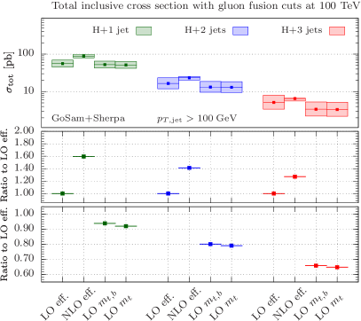
Figure 1: Inclusive cross sections for $\mathrm{H}$ ​+​ 1​ jet, $\mathrm{H}$ ​+​ 2​ jets and $\mathrm{H}$ ​+​ 3​ jets production at center-of-mass energies of $13~{}\mathrm{TeV}$ and $100~{}\mathrm{TeV}$ shown to the left and right, respectively. The width of the bands shows the associated scale uncertainty.

Focusing on the central values, we observe that the leading-order contribution in the effective theory agrees in general very well with the predictions based on the full theory. Taking bottom-quark loops into account leads to corrections, which are as small as one percent for all three final-state multiplicities we are considering, and, as expected, they become even smaller at $100~{}\mathrm{TeV}$. However, it is interesting to note the change in the sign of these corrections with increasing jet multiplicity. While for $\mathrm{H}$ ​+​ 1​ jet production at $13~{}\mathrm{TeV}$ the cross section is reduced when bottom-quark loop contributions are included, for $\mathrm{H}$ ​+​ 2​ jets and $\mathrm{H}$ ​+​ 3​ jets the cross section increases instead. This is clearly visible in the first column of Table 1 and displayed in the second ratio plot on the left in Figure 1. If we compare the predictions at $100~{}\mathrm{TeV}$ given in Table 1 for the two different transverse momentum cuts applied to the jets, we observe a sign flip in the interference effects for $\mathrm{H}$ ​+​ 1​ jet. While for $p_{T,\,\mathrm{jet}}>30~{}\mathrm{GeV}$, the pattern is similar to the $13~{}\mathrm{TeV}$ results, increasing the minimum $p_{T}$ of the jet instead yields a small positive overall contribution once both quark-loop contributions of the heaviest generation are included. This means that the effect of the interference on the cross section is destructive in the low transverse momentum region, whereas at high $p_{T}$ the sum of top-quark and bottom-quark contributions leads to constructive interference effects. We will come back to this in Section 4.2, where we discuss the impact of these interference effects on differential distributions.

4 Heavy-quark mass effects in differential distributions

Recalling the 100 $\mathrm{TeV}$ collider results from Table 1, we have already seen that an increase of the jet $p_{T}$ threshold leads to a noticeable change of the total Higgs boson plus jet cross sections. By studying differential cross sections for various classes of observables, we want to identify the phase-space regions that receive important corrections as a result of the finite-mass treatment of the heavy-quark loops. For a broader understanding of this issue, we consider different scenarios that are of relevance to ongoing and future hadron collider experiments.

4.1 LHC predictions for 13 TeV collisions

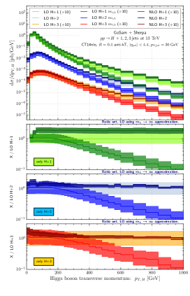
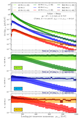
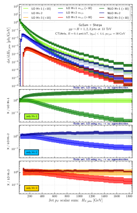
(a) Comparison of effective theory predictions at LO and NLO with LO predictions (indicated by the extra ‘$m_{t,b}$’ label) obtained in the full SM for various observables monitoring the transverse jet activity in the various Higgs boson plus jet production processes. The Higgs boson transverse momentum $p_{T,\,H}$, is shown on the left while the leading jet transverse momentum, $p_{T,\,j_{1}}$, and scalar $p_{T}$ sum of all jets, $H_{T,\,\mathrm{jets}}$, is presented in the middle pane and in the right pane, respectively. Note that the $\mathrm{H}$ ​+​ 1​ jet (green curves) and $\mathrm{H}$ ​+​ 3​ jets (red curves) predictions have been rescaled for better visibility. The smaller plots in the lower part of each panel show the ratios of the three different predictions normalized to the LO effective theory prediction. This is done separately for each of the $\mathrm{H}$ ​+​ 1​ jet, $\mathrm{H}$ ​+​ 2​ jets and $\mathrm{H}$ ​+​ 3​ jets processes.

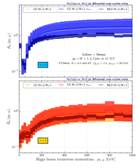
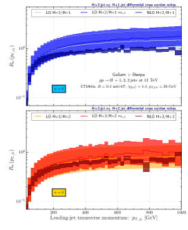
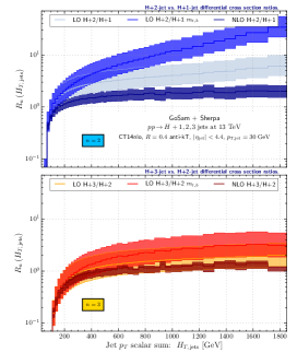
(b) Differential $\mathrm{H}$ ​+​ 2​ jets over $\mathrm{H}$ ​+​ 1​ jet ratios (upper row) and $\mathrm{H}$ ​+​ 3​ jets over $\mathrm{H}$ ​+​ 2​ jets ratios (lower row) for the transverse momentum spectra of the Higgs boson, on the left, and the leading jet, in the middle, as well as the all-jets scalar $p_{T}$ sum, on the right. Each panel shows the ratios for the three theories considered here, the LO and NLO effective theory as well as the full theory at LO.

Figure 2: Various transverse momentum distributions and ratios between successive $n$-jet bins for the production of $\mathrm{H}$ ​+​ $n$​ jets ($n=1,2,3$) at the 13 $\mathrm{TeV}$ LHC.

We start with the discussion of differential distributions relevant for the LHC operated at a collider energy of 13 $\mathrm{TeV}$. In the figures presented here, we compare the effective theory predictions at LO and NLO with results obtained in the full SM. This provides us with a direct comparison of the size of the different corrections. We can decide more easily whether we need to pay attention to including the NLO effects in the effective theory or the finite-mass effects based on the full theory. We are also able to identify observables and/or kinematical environments where it will be mandatory to incorporate both effects in one way or another.

For the full theory calculations, we usually consider both of the heaviest quarks running in the loop, i.e. we take the top quark as well as the bottom quark contributions into account. The associated predictions will hence show the additional label ‘$m_{t,b}$’ in the figures. Depending on the specific observable, we will present all three or two of the $\mathrm{H}$ ​+​ $n$​ jets predictions together in one plot (with $n=3$ being the maximum jet number). In the lower part of these plots, we display for each jet bin separately, the ratios of the three different types of predictions taken with respect to the corresponding LO result in the effective theory. For example, in Figure 2(a), the upper, middle and lower ratio plots show the different ratios based on the predictions for $\mathrm{H}$ ​+​ 1​ jet, $\mathrm{H}$ ​+​ 2​ jets and $\mathrm{H}$ ​+​ 3​ jets, respectively.

Transverse momentum distributions are known to receive significant corrections that lead to a softening of the distribution for larger $p_{T}$ values. We thus investigate this class of observables first, and summarize most of our results in Figure 2. For all three processes, i.e. for the production of $\mathrm{H}$ ​+​ 1​ jet, $\mathrm{H}$ ​+​ 2​ jets and $\mathrm{H}$ ​+​ 3​ jets, Figure 2(a) displays next to each other the transverse momentum distributions of the Higgs boson (left panel) and the hardest jet (center panel), and the scalar sum of the transverse momenta of all jets (right panel). These three distributions clearly show the expected behaviour of $p_{T}$-tail softening. For small transverse momenta (or small $H_{T}$), we find that the leading-order predictions based on the effective theory are in very good agreement with the respective leading-order predictions given by the SM. This is because the heavy top-quark approximation works very well in this low-$p_{T}$ region. Furthermore, we see that this statement holds for all three jet multiplicities considered here. Focusing on the pure $p_{T}$ distributions of Figure 2(a), we observe that the point at which the effective theory approach starts to break down occurs around Higgs boson or lead-jet values of $p_{T}=200~{}\mathrm{GeV}$ and is to a good approximation independent of the jet multiplicity of the Higgs boson production processes. This observation would support a rather simple explanatory model, in which we assume that the resolution of the effective vertex is mainly driven by a quantity, which is very strongly correlated with the event’s hardest single particle $p_{T}$. The inner structure of the $ggH$ vertex will therefore be probed with any interaction where the leading particle-$p_{T}$ exceeds the top-quark mass. In $\mathrm{H}$ ​+​ $n$​ jets production, the hardest particle is either the Higgs boson itself or the leading jet. This right away explains why the breakdown occurs for both the $p_{T,\,H}$ and the $p_{T,\,j_{1}}$ spectra at the same scale. As we will argue further below, this assumption for the main resolution driver seems to also work well for the other examples of transverse observables discussed in this section.

Above the breakdown scale, the deviation from the full SM predictions becomes sizeable very rapidly, resulting in a strong suppression by a factor of 10 at $p_{T}\sim 1~{}\mathrm{TeV}$. Compared to this, the NLO corrections in the effective theory lead to enhancements of the cross section, which are distributed in a relatively uniform way. Since we use $\hat{H}^{\prime}_{T}/2$ as our central scale, the differential $K$-factor between the LO and NLO effective prediction turns out to be flat for the production of $\mathrm{H}$ ​+​ 1​ jet Greiner:2015jha , whereas it has a non-trivial shape for $\mathrm{H}$ ​+​ 2​ jets and $\mathrm{H}$ ​+​ 3​ jets production. The latter two $K$-factors however approach $1$ for transverse momenta that are about or larger than $600~{}\mathrm{GeV}$. It is therefore fair to say that the NLO corrections turn into a subleading effect, already at $p_{T}\sim 400~{}\mathrm{GeV}$, as one has to contrast their behaviour with the strong $p_{T}$ dependence of the finite-mass corrections.

We note that similar observations regarding finite-mass effects have been made before. They have been pointed out in particular for the $p_{T,\,H}$ distribution Buschmann:2014sia ; Frederix:2016cnl ; Badger:2016bpw . In the one-jet case, we can use the leading-order exact statement that $p_{T,\,H}=p_{T,\,j_{1}}$ ($=H_{T,\,\mathrm{jets}}$). It is however interesting to see that the differential ratios associated with $p_{T,\,H}$ and $p_{T,\,j_{1}}$ (see the lower part of Figure 2(a)) are strikingly similar in their characteristics even beyond the one-jet case. In addition, they are also very similar among the different jet bins, suggesting that the relative $1/p^{2}_{T}$ scaling between the effective and full theory at LO can be applied in a more universal manner (cf. Section 1). In fact if we concentrate on the $p_{T,\,H}$ predictions, we observe that the suggested scaling holds to a fairly good extent. For example, at $p_{T,\,H}\approx 400~{}\mathrm{GeV}$, the mass effects reduce the cross section to roughly 60% of the effective theory result. At $p_{T,\,H}>1~{}\mathrm{TeV}$, this reduction then turns into an one-order of magnitude effect, which fixes the related cross section ratio at a value of

$$\dfrac{\tfrac{\mathrm{d}\sigma}{\mathrm{d}p_{T,\,H}}\big{(}p_{T,\,H}=1.0~{}\mathrm{TeV}\big{)}}{\tfrac{\mathrm{d}\sigma}{\mathrm{d}p_{T,\,H}}\big{(}p_{T,\,H}=0.4~{}\mathrm{TeV}\big{)}}\;\approx\;\frac{10\%}{60\%}\;=\;\frac{1}{6}~{}.$$ (9)

The above number (as given by our computation) can be compared with the number one expects from exploiting the relative scaling property between the effective and full theory predictions. Based on the additional suppression of the full result by two powers of $p_{T,\,H}$, the expected value for the same cross section ratio amounts to $(400~{}\mathrm{GeV}/1000~{}\mathrm{GeV})^{2}=4/25$, which is very close to the value extracted from the theory data. This result for the scaling does not change much among the different jet bins because the three ancillary plots in the lower part of Figure 2(a) show that the ratio between full and effective theory predictions only marginally loses some of its steepness for an increasing final-state multiplicity.

The cumulative characteristics of the $H_{T,\,\mathrm{jets}}$ observable shown in the right panel of Figure 2(a) leads to an amplification of the NLO effects in the effective theory (for obvious reasons), while the full theory distributions in the multijet cases fall off less severely at larger scales than they do for the single-object $p_{T}$ spectra discussed above. We also notice that the breakdown of the effective approach occurs at higher scales. In fact an increasing jet multiplicity tames the finite-mass effects further, i.e. yields a weaker scaling and pushes the breakdown scale out to larger values of $H_{T}$. The reason for these changes becomes clear by looking at a fixed $H_{T,\,\mathrm{jets}}$ point, for example $H_{T,\,\mathrm{jets}}=1~{}\mathrm{TeV}$. The transverse hardness is shared among all jets, which also means that the leading jet appears at a scale lower than $1~{}\mathrm{TeV}$. At this lower scale, the deviation of the full theory $p_{T,\,j_{1}}$ prediction has not grown as large as for exactly $1~{}\mathrm{TeV}$. This has to be reflected by the finite-mass $H_{T,\,\mathrm{jets}}$ distribution, which therefore cannot fall as quickly as the $p_{T,\,j_{1}}$ distribution.

As we are interested in the scaling properties of the finite-mass effects, it is beneficial to study the ratios of successive differential jet cross sections. Given a specific observable, we define these ratios as

$$R_{n}(O)\;=\;\dfrac{\dfrac{\mathrm{d}\sigma}{\mathrm{d}O}\big{(}\mathrm{H}\!+\!n\!\mbox{~{}jets}\big{)}}{\dfrac{\mathrm{d}\sigma}{\mathrm{d}O}\big{(}\mathrm{H}\!+\!(n-1)\!\mbox{~{}jets}\big{)}}~{}.$$ (10)

Figure 2(b) visualizes the $R_{2}$ and $R_{3}$ ratios (i.e. the differential ratios for $\mathrm{H}$ ​+​ 2​ jets/$\mathrm{H}$ ​+​ 1​ jet and $\mathrm{H}$ ​+​ 3​ jets/$\mathrm{H}$ ​+​ 2​ jets cross sections) for the transverse momentum observables discussed above. The ratios are shown for each type of our predictions. Figure 2(b) therefore supplements Figure 2(a) greatly, as it clearly exhibits the relative importance of the respective subleading jet multiplicity at higher scales, and the robustness of this feature under finite-mass effects. For all three observables, we essentially find two regimes independent of the type of the prediction: at low transverse scales, the $n$-jet contribution is always significantly smaller than the ($n-1$)-jet contribution, but rises quickly with increasing transverse scales. This has already been pointed out in Ref. Greiner:2015jha . Above a certain scale (which appears around $400~{}\mathrm{GeV}$ for $p_{T,\,H}$ and $p_{T,\,j_{1}}$, and around twice that scale for $H_{T,\,\mathrm{jets}}$), one enters the saturation or scaling regime where the $R_{2}$ and $R_{3}$ can be roughly described by a constant. This indicates (and confirms our earlier statements) that nearly the same scaling is in place in successive jet bins. The largest deviations from this behaviour and between the different predictions can be found for the $R_{2}(H_{T,\,\mathrm{jets}})$, which is no surprise again due to the cumulative nature of the observable. The $R_{2}$ generally level off at higher values than the $R_{3}$ where the inclusion of finite-mass effects yields a slight increase of the respective LO effective ratios. Again, the $R_{2}$ are somewhat more affected by this. The NLO corrections to the effective predictions work in the opposite direction. In all ratio distributions, they stabilize the constant behaviour in the saturation regime.

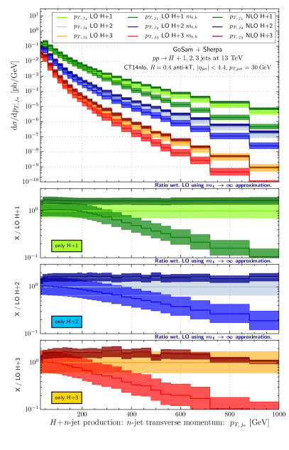
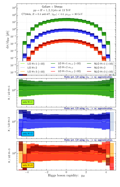
Figure 3: Comparison of the LO and NLO effective theory predictions with the LO predictions in the full SM for the transverse momentum of the $n$-th jet, $p_{T,\,j_{n}}$, in $\mathrm{H}$ ​+​ $n$​ jets production, on the left, and the Higgs boson rapidity, $y_{H}$, on the right. For the three modes of $\mathrm{H}$ ​+​ 1​ jet, $\mathrm{H}$ ​+​ 2​ jets and $\mathrm{H}$ ​+​ 3​ jets production, each column of secondary plots shows the ratios of the three different predictions normalized to the one of the LO effective theory.

Figure 3 depicts, on the left hand side, the transverse momentum distributions of the respective ‘wimpiest’ jet in all three $\mathrm{H}$ ​+​ $n$​ jets channels, i.e. it shows the leading jet in $\mathrm{H}$ ​+​ 1​ jet, the second leading jet in $\mathrm{H}$ ​+​ 2​ jets and the third leading jet in $\mathrm{H}$ ​+​ 3​ jets production. On the right hand side of the same figure, the rapidity distributions of the Higgs boson are presented for the three cases of producing the Higgs boson in association with one jet, two jets or three jets. Compared to the observables discussed so far, the rapidity distributions show a completely different behaviour. Here the full theory and the effective theory agree throughout the entire rapidity range. This is expected since the regions of the phase space where the top-quark loop is resolved are more or less uniformly distributed in rapidity, and their contribution is suppressed by at least one order of magnitude (as shown by the $p_{T}$ spectra in Figure 2(a)) compared to the bulk of events, for which the full and effective theory approaches agree. The NLO corrections regarding the latter are sizeable although they mainly enhance the cross section while leaving the shape more or less unaltered.

As can be seen in the left panel of Figure 3, the effective theory approach starts to deviate at even smaller values of the transverse momentum, namely around $125~{}\mathrm{GeV}$ or $100~{}\mathrm{GeV}$, if one considers the second leading jet in $\mathrm{H}$ ​+​ 2​ jets production or the third leading jet in $\mathrm{H}$ ​+​ 3​ jets production, respectively. This is a consequence of the $p_{T}$ ordering of the jets. In both cases there has to be a harder jet present in the event that is distributed according to $\mathrm{d}\sigma/\mathrm{d}p_{T,\,j_{n-1}}$. For the leading jet in $\mathrm{H}$ ​+​ 2​ jets and $\mathrm{H}$ ​+​ 3​ jets events, the deviation between the effective and full theory results begins around $200~{}\mathrm{GeV}$ (see center panel in Figure 2(a)). The distributions for the second hardest jet must therefore deviate around $(200-X)~{}\mathrm{GeV}$ where $X>0$, and similarly, for $\mathrm{H}$ ​+​ 3​ jets final states, the third-jet distribution must break down around $(200-X-Y)~{}\mathrm{GeV}$ where $Y>0$. Hence, the $p_{T}$ ordering of the jets translates into an ordering of breakdown scales. In other words, if the superior jet does not resolve the heavy-quark loop, the softer one will not do so at all.

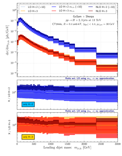
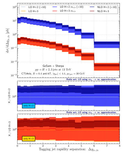
Figure 4: Theoretical predictions based on the LO and NLO effective and the full approach at LO for the invariant mass (left) and the rapidity separation (right) of the two leading jets in $\mathrm{H}$ ​+​ 2​ jets and $\mathrm{H}$ ​+​ 3​ jets production. The layout of the plots corresponds to that of Figure 2(a).

For the two-jet and three-jet processes, it is interesting to study the invariant mass spectrum between the two hardest jets, which are also the tagging jets in the $p_{T}$ jet-tagging scheme. This observable plays an important role in the definition of kinematic constraints for VBF analyses. The other key observable needed in VBF studies is the rapidity separation of the same pair of jets. Both distributions are shown in Figure 4 for $\mathrm{H}$ ​+​ 2​ jets and $\mathrm{H}$ ​+​ 3​ jets final states. For the invariant mass distribution, one observes only a mild deviation between the full and the effective theory predictions, which becomes more pronounced towards the higher end of the kinematical range. As a matter of fact, large invariant tag-jet masses are not only generated in events with hard tagging jets. The geometry of the momentum flow is an important criteria for the production of dijet masses. For example, in a situation where the two jets appear in a back-to-back configuration, large invariant masses can emerge despite the absence of energetic jets. In these cases, the effect of the heavy quarks is significantly reduced, and the effective theory therefore can be used to describe this observable accurately.

For the rapidity separation between the two tagging jets, shown on the right hand side in Figure 4, the situation is similar to that of the rapidity distribution of the Higgs boson discussed above. It is therefore clear that there is a good agreement between the effective theory and the full theory predictions for this observable.

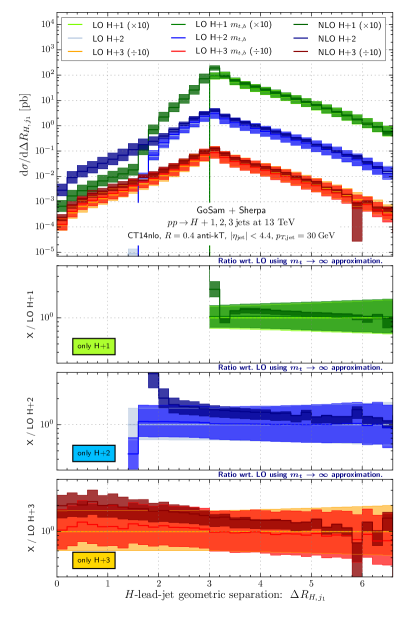
Figure 5: Theoretical predictions based on the LO and NLO effective and the full approach at LO for the geometric separation, in terms of radial distances, between the Higgs boson and the leading transverse momentum jet (left panel), and between the Higgs boson and the closest jet in the event (right panel). The layout of the plots corresponds to one used in Figure 2(a).

Figure 5 shows on the left hand side the radial separation $\Delta R_{H,\,j_{1}}$ between the Higgs boson and the leading jet. On the right hand side, we display the smallest of the radial distances between the Higgs boson and any of the jets in the event, $\Delta R_{\mathrm{min},\,H,\,j_{k}}$. In $\mathrm{H}$ ​+​ 1​ jet production at LO, the Higgs boson and the only jet present in the event are forced into a back-to-back configuration. The $\Delta R_{H,\,j_{1}}$ distribution has therefore a natural cut-off at $\pi$, where it also peaks. At NLO, the presence of a second jet, which can become unresolved, opens up the previously kinematically forbidden range between $0$ and $\pi$. The $\mathrm{H}$ ​+​ 2​ jets distribution at LO also has a kinematical constraint owing to the presence of two jets that must be resolved. The radial distance between the Higgs boson and the leading jet can therefore not be smaller than the minimal azimuthal angle of $\Delta\phi=\pi/2$. The presence of at least a third jet (in $\mathrm{H}$ ​+​ 2​ jets final states at NLO and $\mathrm{H}$ ​+​ 3​ jets final states) allows one to finally populate the full kinematical spectrum. From the distributions, it is however clear that the Higgs boson preferably recoils against the leading jet, because independent of the jet multiplicity, the distributions are all peaked at $\Delta R_{H,\,j_{1}}=\pi$. The finite-mass effects are only very mild in the $\mathrm{H}$ ​+​ 1​ jet and $\mathrm{H}$ ​+​ 2​ jets case. In the $\mathrm{H}$ ​+​ 3​ jets case, they give a small correction that slightly increases the cross section at small radial separation, and decreases it at values larger than $\Delta R_{H,\,j_{1}}=\pi$. This is a consequence of $\Delta R$ being derived from the rather robust variables $\Delta y$ and $\Delta\phi$.

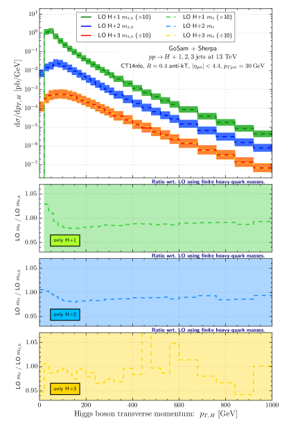
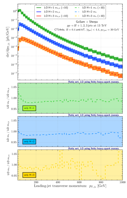
Figure 6: Transverse momentum distributions of the Higgs boson (left) and leading transverse momentum jet (right). The curve show predictions in the full standard model with and without additional bottom-quark loops for the three studied jet multiplicity. The width of the band represents the scale uncertainty. The lower plots show the ratio between the two central values. Because of the very small differences the edges of the scale uncertainty band is not visible in the lower plots.

For the same reason mentioned previously, the minimal radial separation between the Higgs boson and a jet has a kinematic edge at $\pi$ in $\mathrm{H}$ ​+​ 1​ jet production at LO. In all other cases, the distribution is spread over the entire kinematical range. It is interesting to notice that, contrary to the plot on the left, in the $\mathrm{H}$ ​+​ 2​ jets and $\mathrm{H}$ ​+​ 3​ jets final states, the distributions flatten out for $\Delta R_{\mathrm{min},\,H,\,j_{k}}$ values between $2$ and $\pi$. Based on these and earlier findings, a typical event where the Higgs boson is produced in association with several jets will likely have these features: the Higgs boson will tend to recoil against the leading jet, but clearly, as the multiplicity increases, it will occur more often in company of a close, rather soft jet. Finally we remark on the good agreement between the predictions from the effective theory and the predictions including the mass corrections. Only for $\mathrm{H}$ ​+​ 3​ jets production, and for large radial separations between the jets do the two curves start to deviate. In contrast to this, the NLO corrections in the effective approach have a significantly larger impact, and this statement extents to all 2-body correlations considered in this section.

4.2 The case of massless bottom quarks

In this section we compare the predictions for differential distributions in the full theory with and without the $b$-quark loop contribution, with the aim to assess the effects of neglecting the bottom quark contribution. In Table 1 and Figure 1 above we already commented the impact on the total cross sections, and observed a change in the sign of these contribution between the $\mathrm{H}$ ​+​ 1​ jet predictions and $\mathrm{H}$ ​+​ 2​ jets and $\mathrm{H}$ ​+​ 3​ jets predictions. This can now be quantified better at the differential level.

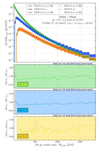
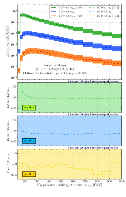
Figure 7: Same as Fig. 6, but for the scalar sum of the jet transverse momenta and the invariant mass of the Higgs boson and the leading transverse momentum jet.

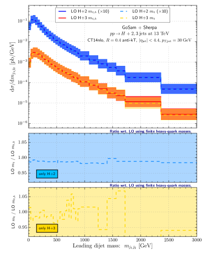
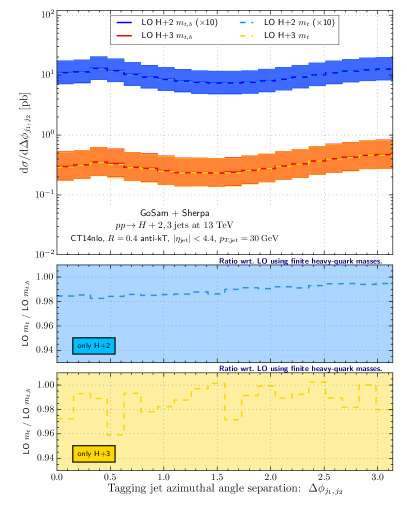
Figure 8: Same as Fig. 6, but for the invariant mass of the leading dijet system (left) and their azimuthal angle separation (right).

For this we focus our attention on a few selected observables. In Figure 6 we show the Higgs boson and the leading jet transverse momenta, in Figure 7 we compare the scalar sum of the jet transverse momenta $H_{T,\mathrm{jets}}$ and the invariant mass of Higgs boson and leading transverse momentum jet, whereas in Figure 8 we plot the invariant mass of the tagging jets and their azimuthal angle difference $\Delta\phi_{j1,j2}$. All the plots show the corresponding observable as well as ratio plots for the three different jet-multiplicities. The ratio is given by the result in which only top-quark loops are considered, divided by the predictions where both top- and bottom-quark contributions are taken into account. The color shaded areas denote the scale uncertainty. For a better visibility we do not show the full scale uncertainty band in the ratios, but rather zoom in around the central scale.

It is clearly visible that the scale uncertainty outweighs the bottom mass effects by far, for all the considered observables. The size of the effects strongly depends on the observable but never exceeds five percent. In general, the bottom-quark mass effects are most visible in the observables involving transverse momenta and sums thereof and in invariant masses involving the Higgs. It is however interesting to observe which of the two predictions is larger as a function of the kinematical region considered. The largest effects can be observed in the soft region of the observables. This is to be expected, since especially when the kinematical scales involved are not too large compared to the bottom-quark mass, bottom-quark loops can lead to sizable corrections to the predictions in which only the top quark is considered. Far away from these kinematic regions the bottom quark can be considered massless. Furthermore, as already discussed in section 3, the size and sign of the effect depends on the jet multiplicity. This can be seen for instance in Figure 7. The destructive interference for $\mathrm{H}$ ​+​ 1​ jet at the level of the total cross section stems from the soft region, whereas the net contribution becomes positive in regions where the b-quark can be considered massless. For $\mathrm{H}$ ​+​ 2​ jets and $\mathrm{H}$ ​+​ 3​ jets the destructive interference is considerably reduced, leading to an increase of the total cross section when bottom-quark loops are taken into account. For angular variables these contributions are instead flat, over the whole kinematical range. This is expected since the effects are uniformly distributed in these variables as already discussed in the previous section.

4.3 VBF measurements at the LHC

The production of a Higgs boson in association with two or more jets in the gluon-fusion channel is also the main background to the VBF production channel. Since the latter has a very characteristic topological signature, in which two jets are produced mainly at high rapidities with a large invariant mass and a large azimuthal separation, leaving little jet activity in the central region of the detector, this channel can be enhanced with respect to the background by additional cuts, similar to the one of Eq. 8. In this section we investigate the impact of the mass effects on the gluon-fusion predictions when these additional cuts are applied.

Numbers in [pb]	$\mathrm{H}\!+\!2$ jets|	$\mathrm{H}\!+\!3$ jets|
$\sigma_{\mathrm{LO,\,eff.}}$ |	$0.397^{+64\%}_{-36\%}$	$0.166^{+82\%}_{-42\%}$
$\sigma_{\mathrm{NLO,\,eff.}}$ |	$0.584^{+10\%}_{-19\%}$	$0.231^{+5\%}_{-22\%}$
$\sigma_{\mathrm{LO},\,m_{t,b}}$ |	$0.404^{+65\%}_{-37\%}$	$0.167^{+82\%}_{-42\%}$
$\sigma_{\mathrm{LO},\,m_{t}}$ |	$0.398^{+65\%}_{-37\%}$	$0.165^{+82\%}_{-42\%}$

Table 2: Total inclusive cross sections for the production of a Higgs boson in association with two or three jets at LO and NLO in QCD in the effective theory and at LO in the full SM for massive top- and bottom-quarks and for massive top quarks only. Numbers are reported for center-of-mass energies of 13 $\mathrm{TeV}$. In addition to the jet transverse momentum cut of $p_{T,\,\mathrm{jet}}>30~{}\mathrm{GeV}$, we demand $m_{j_{1}j_{2}}\,>\,400~{}\mathrm{GeV}$ and $\left|\Delta y_{j_{1},\,j_{2}}\right|\,>\,2.8$. The uncertainty estimates are obtained from standard scale variations.

As already demonstrated by Figure 4, both the $m_{j_{1}j_{2}}$ variable and the $\Delta y_{j_{1},j_{2}}$ variable are almost unaffected by mass corrections. We can therefore expect that at the level of the total cross section the pattern stays similar as the case without VBF cuts. The total cross sections reported in Table 2 confirm this. Also the effect of the massive bottom-quark loops is very small leading to changes in range of $1-2\%$. Therefore, for the remainder of this section, we will not discriminate between top-quark only and combined top-quark and bottom-quark effects, instead always include both massive quark loop contributions at the same time.

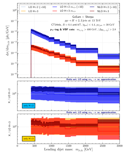
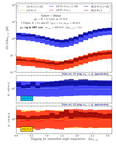
Figure 9: Leading dijet invariant mass distribution (left) and azimuthal angle separation of the tagging jets (right) passing the VBF selection cuts.

Two of the key observables in the VBF scenario are the invariant mass distribution of the tagging jets $m_{j_{1}j_{2}}$ and their azimuthal angular separation $\Delta\phi_{j_{1},j_{2}}$ . These two observables are shown in Figure 9. The comparison between the full theory and the effective theory predictions reveals a good agreement between the two, indicating that mass effects are rather small.

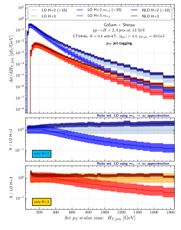
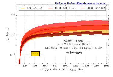
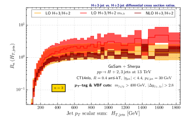
Figure 10: The distribution of the scalar transverse momentum sum of all jets in H+2-jet and H+3-jet events before and after passing the VBF selection cuts.

These effects become, however, considerably larger when one considers observables that have already been seen to be sensitive to heavy-quark loops in the previous sections. In Figure 10 we show the scalar sum of the transverse momenta $H_{T,\mathrm{jets}}$ of the jets before (left hand side) and after applying the VBF cuts (right hand side). The effect is clearly visible when comparing the ratio plots normalized to the LO in the effective theory: after VBF cuts the mass effects become more severe, leading to larger deviations of the effective theory from the full theory for high transverse momenta. In the lowest row we show the differential ratio between $\mathrm{H}$ ​+​ 3​ jets and $\mathrm{H}$ ​+​ 2​ jets, which remains roughly unchanged.

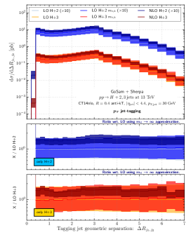
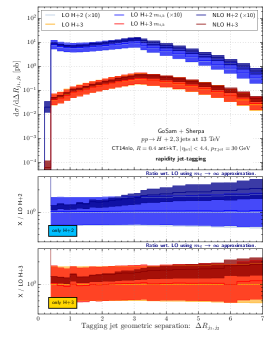
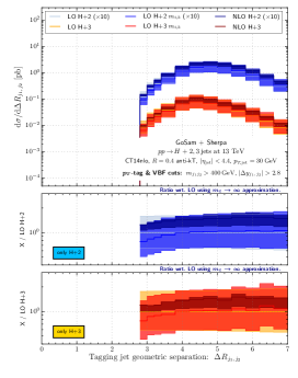
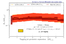
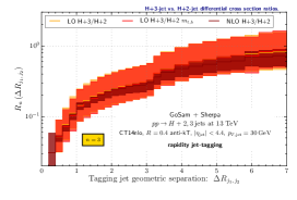
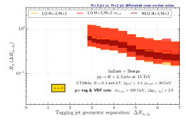
Figure 11: Geometric separation of the tagging jets in $\mathrm{H}$ ​+​ 2​ jets and $\mathrm{H}$ ​+​ 3​ jets events when applying only baseline cuts in the $p_{T}$-jet tagging (left panel), for baseline cuts with rapidity ordering (middle panel) and when applying additional VBF cuts in the $p_{T}$ jet-tagging scheme (right panel).

Another important observable is the radial separation between the two tagging jets $\Delta R_{j_{1},j_{2}}$. This observable is considered in Figure 11. On the left and in the middle column we show this observable before applying VBF cuts. The first plot shows the observable for a $p_{T}$ jet-tagging, whereas in the second plot we adopt a $y$ jet-tagging strategy. Although NLO effects in the effective theory lead to substantial differences between the two tagging schemes, the two leading order results in the full and the effective theory agree very well for both tagging schemes and for both multiplicities. At least at leading order the choice of the tagging scheme is therefore insensitive to mass effects. The plot on the right hand side shows the observable using the original $p_{T}$ jet-tagging but after applying VBF cuts. In this case mass corrections have an impact especially for $\Delta R\approx 3$ , where deviations can become larger than $20\%$. When the two jets are not too far in radial distance, the Higgs boson must in general be harder and recoil against them. This explains the discrepancy between the two LO predictions. The bottom plots show the ratio between the two jet multiplicities. As expected, both the tagging scheme as well as the VBF cuts have a significant impact on this ratio. However, heavy-quark mass effects do not lead to deviations from the prediction of the effective theory.

4.4 FCC predictions for 100 TeV collisions

In view of a possible future circular collider operating at a center-of-mass energy of $100$ $\mathrm{TeV}$, we also investigate the mass effects for such a high collider energy. Values for the total cross section at the different multiplicities were already presented and discussed above in Section 3 and Table 1. In this section we focus on differential distributions.

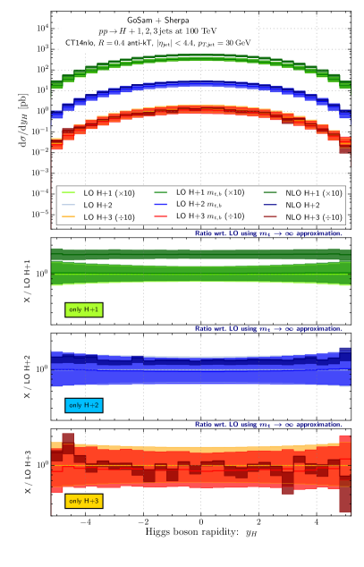
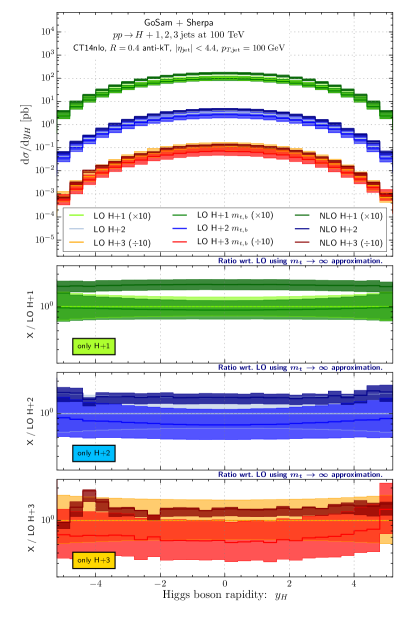
Figure 12: The Higgs boson rapidity distribution for a low and high jet $p_{T}$ threshold.

In Figure 12 we investigate the impact of the mass effects depending on the cut on the jets transverse momentum by looking at the Higgs boson rapidity distribution. On the left the transverse momentum cut on the jets is $p_{T,\,\mathrm{jet}}>30$ $\mathrm{GeV}$, whereas on the right it is increased to $p_{T,\,\mathrm{jet}}>100$ $\mathrm{GeV}$. At $13$ $\mathrm{TeV}$ the leading order contributions of the full and the effective theory agree very well and we find the same good agreement at 100 $\mathrm{TeV}$ for the looser transverse momentum cut. Requiring a minimum transverse momentum of $100$ $\mathrm{GeV}$ leads to visible deviations between full and effective theory. This is clearly related to the fact that the bulk of the cross section comes from the softest allowed region of the phase space, where the mass effects play only a very minor role. Increasing the $p_{T}$ threshold, however, cuts away this large and mass-insensitive part of the cross section and the remaining contribution is much more affected by mass effects.

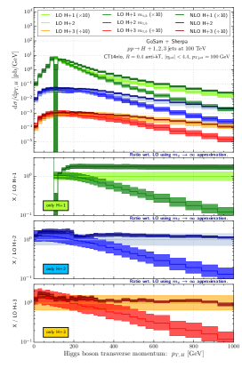
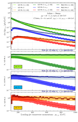
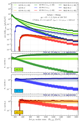
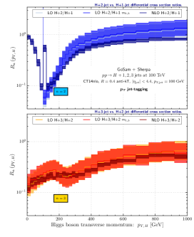
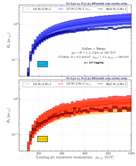
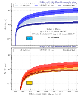
Figure 13: Various transverse momentum distributions for the three Higgs boson plus $n$-jet bins and their associated successive jet bin ratios.

In Figure 13 we show the transverse momentum of the Higgs and the leading jet as well as $H_{T}$ of the jets with a $p_{T}$ cut on the jets of $100$ $\mathrm{GeV}$. Owing to the increase in the cross section and the possibility to produce much harder jets and Higgs bosons, all these observables suffer from large mass effects, which for transverse momenta larger than $1$ $\mathrm{TeV}$ lead to corrections which are bigger than one order of magnitude. The lowest panel shows the inclusive differential $\mathrm{H}$ ​+​ 2​ jets/$\mathrm{H}$ ​+​ 1​ jet and $\mathrm{H}$ ​+​ 3​ jets/$\mathrm{H}$ ​+​ 2​ jets ratios for the three different observables. These ratios remain unchanged for the transverse momentum of the Higgs boson, meaning that the relative importance of higher multiplicity contributions is stable under mass effect corrections, and we also see an only very mild deviation for the transverse momentum of the leading jet. However, for $H_{T}$ the ratio increases when passing from the effective theory predictions to the full SM. The massive quark loop effects are therefore stronger in the high transverse momentum tails for the lower multiplicities than for the higher ones.

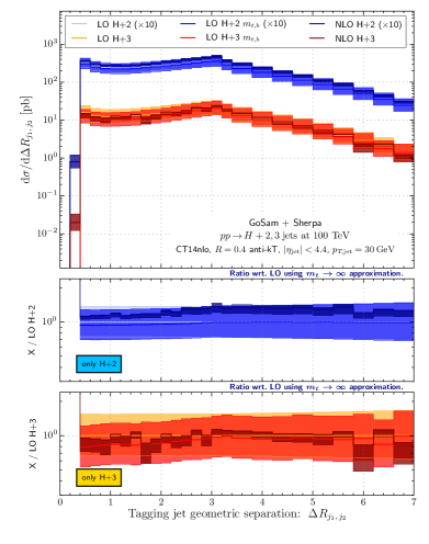
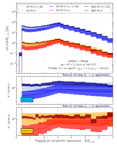
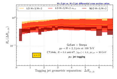
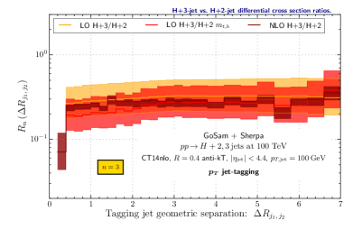
Figure 14: Geometric separation between the leading jets for a low and high jet threshold and the associated $R_{3}$ ratios using $p_{T}$ jet-tagging.

Figure 14 shows again the radial separation between the two leading jets $\Delta R_{j_{1},j_{2}}$, this time for 100 $\mathrm{TeV}$ center of mass energy. The two plots show the impact of the finite mass corrections when the minimum transverse momentum threshold is raised from $p_{T,\,\mathrm{jet}}>30$ $\mathrm{GeV}$ to $p_{T,\,\mathrm{jet}}>100$ $\mathrm{GeV}$. The very small differences between the effective theory predictions and the full SM curve at 13 $\mathrm{TeV}$ (Figure 11 – left) become larger, especially for $\mathrm{H}$ ​+​ 3​ jets, when increasing the collider energy, even if the cuts are kept equal. On the lowest ratio of the left plot we observe a non-trivial shape of the mass corrections, which are minimal when the separation is about $\Delta R_{j_{1},j_{2}}\approx\pi$. For smaller separations the two leading jets must be close in the $(y,\phi)$-plane and combine such that the momentum flow through the effective vertex is increased, leading to a break down of the effective theory prediction. The tiny variations in the shape of the mass corrections dramatically increase when the transverse momentum of the jets is required to be above $100$ $\mathrm{GeV}$. The plots on the right reveal a very non-trivial dependence of the mass corrections from the radial distance, and overall the impact of these corrections is much larger than the NLO corrections in the effective theory.

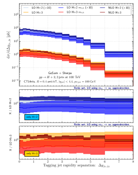
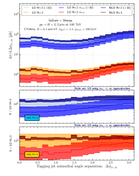
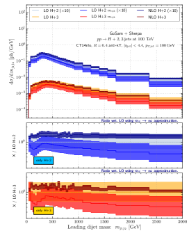
Figure 15: Rapidity and azimuthal angle separation between the leading jets as well as the leading dijet mass for the higher jet threshold.

As can easily be foreseen, the increased deviation of the full SM predictions from the effective theory is present in the observables that we will discuss in the following. We will only present plots for which $p_{T,\,\mathrm{jet}}>100$ $\mathrm{GeV}$, where the effects are much more visible. In Figure 15 we present the two components which combined give rise to the radial distance discussed above: on the left the rapidity separation $\Delta y_{j_{1},j_{2}}$ and in the center the azimuthal angle separation $\Delta\phi_{j_{1},j_{2}}$ between the two leading jets. In the former case the mass corrections are roughly constant over the full kinematical range, whereas in the latter case they are much larger for small angle separation, and become almost negligible when the two jets are back-to-back in azimuth. The reason is similar to the one outlined previously for $\Delta R_{j_{1},j_{2}}$. On the right of the same figure we show the leading invariant dijet mass. As already stressed previously, this observable is particularly important when studying VBF scenarios. Compared to the curve shown for 13 $\mathrm{TeV}$ and a transverse momentum cut of 30 $\mathrm{GeV}$ (Fig. 4), where the mass corrections barely affected the distribution, we observe now a clear decrease of the cross section, which reaches $-50\%$ for invariant masses of the order of $3$ $\mathrm{TeV}$.

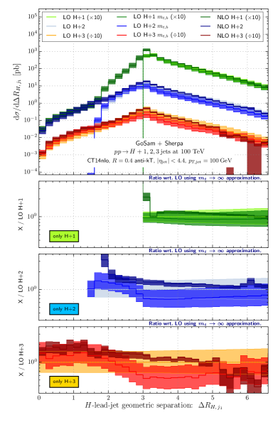
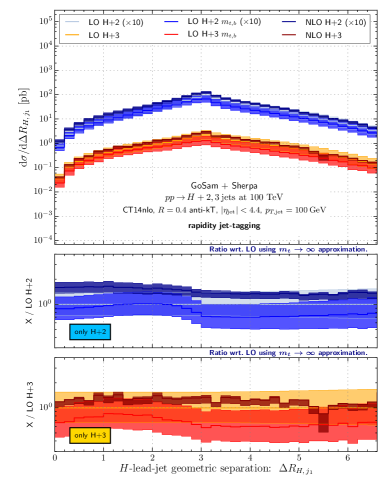
Figure 16: Geometric separation between the Higgs boson and the leading transverse momentum jet for $p_{T,\,\mathrm{jet}}>100$ $\mathrm{GeV}$ and using $p_{T}$-jet tagging (left) as well as $y$-jet tagging (right).

Figure 16 shows the radial separation between the Higgs boson and the leading jet for the two different jet tagging strategies. The plot on the left shows $\Delta R_{H,j_{1}}$ when using a $p_{T}$-jet tagging strategy, whereas on the right we apply the $y$-jet tagging, which by definition needs the presence of at least two jets. This observable demonstrates that mass effects can lead to fairly complicated corrections with respect to the effective theory predictions. Apart from the $\mathrm{H}$ ​+​ 1​ jet predictions, which because of the presence of only a single jet are not affected too much by mass corrections, the full SM predictions increase the cross section at small radial distance and decrease it for larger values of $\Delta R_{H,j_{1}}$. The differences are slightly milder in the right plot when considering a $y$-jet tagging strategy. This is due to the fact that the tagging jets in the rapidity tagging are not necessarily hard jets, which means that the phase space region of hard jets is rather diluted across the observable.

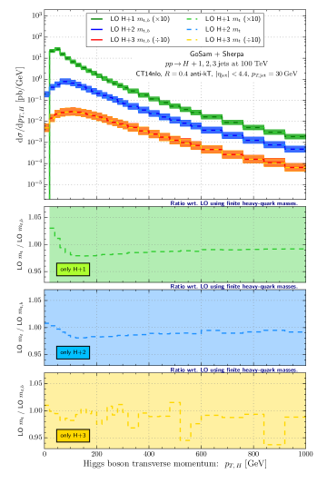
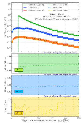
Figure 17: Same as Fig. 6-left but for a center-of-mass energy of 100 $\mathrm{TeV}$ and for $p_{T,\,\mathrm{jet}}>30$ $\mathrm{GeV}$ (left) and $p_{T,\,\mathrm{jet}}>100$ $\mathrm{GeV}$ (right).

To conclude we compare the Higgs boson transverse momentum using full SM predictions with and without bottom-quark loops. Figure 17 shows the two results for a minimum jet transverse momentum of $p_{T,\,\mathrm{jet}}>30$ $\mathrm{GeV}$ on the left, and for $p_{T,\,\mathrm{jet}}>100$ $\mathrm{GeV}$ on the right. The ratios allow to appreciate the difference between the two predictions, which is relevant mainly for $\mathrm{H}$ ​+​ 1​ jet and when the looser jet cut is used. Increasing the jet cut or the final state multiplicity leads to a flatter ratio in which the predictions with only top-quark loops are lower than the one with top- and bottom-quark by $0.5-2\%$.

5 Conclusions

The production of a Higgs boson in association with jets in gluon fusion is one of the key processes in precision Higgs physics. Accurate theoretical predictions are fundamental for a detailed understanding of the electroweak symmetry breaking mechanism. Usually calculations of higher order corrections to the production of a Higgs boson in association with jets rely on the approximation of an infinitely heavy top quark. In this paper we have computed the cross section at LO in perturbation theory in the full Standard Model considering a Higgs boson coupling to both top-quark and bottom-quark loops, including the interference between the two. Furthermore we have compared these results to the NLO predictions in the effective theory approach. We give quantitative predictions for a variety of observables for $\mathrm{H}$ ​+​ 1​ jet, $\mathrm{H}$ ​+​ 2​ jets and $\mathrm{H}$ ​+​ 3​ jets, confirming that transverse-momentum related observables are particularly affected by these corrections for values above the top mass. We have calculated predictions for two center-of-mass energies, for the LHC at $13$ $\mathrm{TeV}$ and for a possible future circular collider of $100$ $\mathrm{TeV}$. For the LHC, we also investigated the impact of finite mass effects when VBF selections cuts are applied on the tagging jets, in order to enhance the VBF signal. We find that mass effects typically play an important role leading to deviations up to one order of magnitude. The breakdown of the effective theory predictions is driven by the particle with the highest transverse momentum in the event and is largely independent of the final state multiplicity. This is of course highly dependent on the specific observable and scenario under consideration. In particular, since the corrections affect the harder transverse momentum regions, choosing a harder $p_{T}$-cut in the analysis results in larger mass effects for all observables. We further find that the effect of including massive bottom-quarks in the loop has a mild impact. For the total cross section, the bottom-quark contribution (including its interference with top-quark loops) is around one percent for a $13$ $\mathrm{TeV}$ LHC. Applying VBF cuts does not lead to significant changes, which is also true for pp-collisions at a $100$ $\mathrm{TeV}$ collider. The bottom-quark effects are particularly visible in the low energy region, where they can lead to deviations of up to five percent.

In summary, the inclusion of mass effects and their control at an accuracy beyond leading order will be indispensable for reliable predictions for both the LHC, but even more for a future collider with considerably higher center-of-mass energy.

Appendix A Root Ntuples

In this section we briefly describe an extension of the Ntuples format, which was introduced recently and partially used for the study presented here.

The original information stored in the Ntuples entries is summarized in Table 3. Recently it was however realized, that a small upgrade could lead to a broader range of applicability and to more flexibility. This was mainly driven by the wish of being able to apply a MiNLO-type Hamilton:2012np ; Badger:2016bpw scale setting on the events stored in the Ntuples. Furthermore, it is of advantage to have the possibility to change a posteriori the matrix element weight stored in the Ntuples, while keeping the same set of events.

Branch	Description
id	Event ID to identify correlated real sub-events
nparticle	Number of outgoing partons
E/px/py/pz	Momentum components of the partons
kf	Parton PDG code
weight	Event weight, if sub-event is treated independently
weight2	Event weight, if correlated sub-events are treated as single event
me_wgt	ME weight (w/o PDF), corresponds to ’weight’
me_wgt2	ME weight (w/o PDF), corresponds to ’weight2’
id1	PDG code of incoming parton 1
id2	PDG code of incoming parton 2
fac_scale	Factorisation scale
ren_scale	Renormalisation scale
x1	Bjorken-x of incoming parton 1
x2	Bjorken-x of incoming parton 2
x1p	x’ for I-piece of incoming parton 1
x2p	x’ for I-piece of incoming parton 2
nuwgt	Number of additional ME weights for loops and integrated subtraction terms
usr_wgt[nuwgt]	Additional ME weights for loops and integrated subtraction terms

Table 3: Branches format of the Ntuples files as generated by Sherpa.

These two requirements led to the development of a new Ntuple format which we will refer to as EDNtuples (Exact Double Ntuples). In this new format an entry called ncount, was introduced, which keeps track of the number of trials between two good events during generation. This allows for an exact statistical treatment when events are reprocessed a posteriori. Furthermore the momenta are stored in double precision instead of float, to allow for a more precise kinematical reconstruction. This is needed for example when the branching history of an event is reconstructed for the MiNLO scale choice. Furthermore, in order to correctly map the subtraction counter-events to the appropriate real radiation events when performing the clustering in MiNLO, additional branches to store the information on the initial state flavours in the subtraction events had to be created. Finally, to be able to change the matrix element weight a posteriori, the phase space weight, which is already multiplied with the weight coming from the amplitude in the branches called me_wgt and me_wgt2, is now also stored separately, giving the possibility to change the weight of the amplitude. This last extension was of particular interests for this work since the events stored in the Ntuples could be reused when computing the amplitude in the full Standard Model theory, when the heavy quark loops are present at LO accuracy. The new entries added in the EDNtuples are summarized in Table 4.

Branch	Description
ncount	Number of trials between the previous and current event during generation
ps_wgt	Phase space weight
id1p	PDG code of incoming parton 1 in subtraction event
id2p	PDG code of incoming parton 2 in subtraction event

Table 4: Additional new branches introduced for the EDNtuples.

References

- (1) F. Wilczek, Decays of Heavy Vector Mesons Into Higgs Particles, Phys.Rev.Lett. 39 (1977) 1304.
- (2) S. Catani, M. Ciafaloni and F. Hautmann, High-energy factorization and small x heavy flavor production, Nucl. Phys. B366 (1991) 135–188.
- (3) F. Hautmann, Heavy top limit and double logarithmic contributions to Higgs production at m(H)**2 / s much less than 1, Phys. Lett. B535 (2002) 159–162, [hep-ph/0203140].
- (4) R. S. Pasechnik, O. V. Teryaev and A. Szczurek, Scalar Higgs boson production in a fusion of two off-shell gluons, Eur. Phys. J. C47 (2006) 429–435, [hep-ph/0603258].
- (5) S. Marzani, R. D. Ball, V. Del Duca, S. Forte and A. Vicini, Higgs production via gluon-gluon fusion with finite top mass beyond next-to-leading order, Nucl. Phys. B800 (2008) 127–145, [0801.2544].
- (6) S. Forte and C. Muselli, High energy resummation of transverse momentum distributions: Higgs in gluon fusion, JHEP 03 (2016) 122, [1511.05561].
- (7) F. Caola, S. Forte, S. Marzani, C. Muselli and G. Vita, The Higgs transverse momentum spectrum with finite quark masses beyond leading order, 1606.04100.
- (8) H. Georgi, S. Glashow, M. Machacek and D. V. Nanopoulos, Higgs Bosons from Two Gluon Annihilation in Proton Proton Collisions, Phys.Rev.Lett. 40 (1978) 692.
- (9) U. Baur and E. W. N. Glover, Higgs Boson Production at Large Transverse Momentum in Hadronic Collisions, Nucl. Phys. B339 (1990) 38–66.
- (10) A. Djouadi, M. Spira and P. Zerwas, Production of Higgs bosons in proton colliders: QCD corrections, Phys.Lett. B264 (1991) 440–446.
- (11) M. Spira, A. Djouadi, D. Graudenz and P. Zerwas, Higgs boson production at the LHC, Nucl.Phys. B453 (1995) 17–82, [hep-ph/9504378].
- (12) V. Del Duca, W. Kilgore, C. Oleari, C. Schmidt and D. Zeppenfeld, Higgs + 2 jets via gluon fusion, Phys.Rev.Lett. 87 (2001) 122001, [hep-ph/0105129].
- (13) V. Del Duca, W. Kilgore, C. Oleari, C. Schmidt and D. Zeppenfeld, Gluon fusion contributions to H + 2 jet production, Nucl.Phys. B616 (2001) 367–399, [hep-ph/0108030].
- (14) F. Campanario and M. Kubocz, Higgs boson production in association with three jets via gluon fusion at the LHC: Gluonic contributions, Phys.Rev. D88 (2013) 054021, [1306.1830].
- (15) M. Buschmann, D. Goncalves, S. Kuttimalai, M. Schonherr, F. Krauss and T. Plehn, Mass Effects in the Higgs-Gluon Coupling: Boosted vs Off-Shell Production, JHEP 02 (2015) 038, [1410.5806].
- (16) R. Frederix, S. Frixione, E. Vryonidou and M. Wiesemann, Heavy-quark mass effects in Higgs plus jets production, 1604.03017.
- (17) K. Melnikov and A. Penin, On the light quark mass effects in Higgs boson production in gluon fusion, JHEP 05 (2016) 172, [1602.09020].
- (18) Editors et al., Physics at a 100 TeV pp collider: Higgs and EW symmetry breaking studies, 1606.09408.
- (19) G. Cullen, H. van Deurzen, N. Greiner, G. Luisoni, P. Mastrolia et al., Next-to-Leading-Order QCD Corrections to Higgs Boson Production Plus Three Jets in Gluon Fusion, Phys.Rev.Lett. 111 (2013) 131801, [1307.4737].
- (20) N. Greiner, S. Hoeche, G. Luisoni, M. Schonherr, J.-C. Winter et al., Phenomenological analysis of Higgs boson production through gluon fusion in association with jets, 1506.01016.
- (21) G. Cullen, N. Greiner, G. Heinrich, G. Luisoni, P. Mastrolia et al., Automated One-Loop Calculations with GoSam, Eur.Phys.J. C72 (2012) 1889, [1111.2034].
- (22) G. Cullen, H. van Deurzen, N. Greiner, G. Heinrich, G. Luisoni et al., GS-2.0: a tool for automated one-loop calculations within the Standard Model and beyond, Eur.Phys.J. C74 (2014) 3001, [1404.7096].
- (23) P. Nogueira, Automatic Feynman graph generation, J.Comput.Phys. 105 (1993) 279–289.
- (24) J. Vermaseren, New features of FORM, math-ph/0010025.
- (25) J. Kuipers, T. Ueda, J. Vermaseren and J. Vollinga, FORM version 4.0, Comput.Phys.Commun. 184 (2013) 1453–1467, [1203.6543].
- (26) G. Cullen, M. Koch-Janusz and T. Reiter, Spinney: A Form Library for Helicity Spinors, Comput.Phys.Commun. 182 (2011) 2368–2387, [1008.0803].
- (27) T. Reiter, Optimising Code Generation with haggies, Comput.Phys.Commun. 181 (2010) 1301–1331, [0907.3714].
- (28) P. Mastrolia, E. Mirabella and T. Peraro, Integrand reduction of one-loop scattering amplitudes through Laurent series expansion, JHEP 1206 (2012) 095, [1203.0291].
- (29) T. Peraro, Ninja: Automated Integrand Reduction via Laurent Expansion for One-Loop Amplitudes, 1403.1229.
- (30) H. van Deurzen, G. Luisoni, P. Mastrolia, E. Mirabella, G. Ossola et al., Multi-leg One-loop Massive Amplitudes from Integrand Reduction via Laurent Expansion, JHEP 1403 (2014) 115, [1312.6678].
- (31) G. Ossola, C. G. Papadopoulos and R. Pittau, Reducing full one-loop amplitudes to scalar integrals at the integrand level, Nucl.Phys. B763 (2007) 147–169, [hep-ph/0609007].
- (32) P. Mastrolia, G. Ossola, C. Papadopoulos and R. Pittau, Optimizing the Reduction of One-Loop Amplitudes, JHEP 0806 (2008) 030, [0803.3964].
- (33) G. Ossola, C. G. Papadopoulos and R. Pittau, On the Rational Terms of the one-loop amplitudes, JHEP 0805 (2008) 004, [0802.1876].
- (34) P. Mastrolia, G. Ossola, T. Reiter and F. Tramontano, Scattering AMplitudes from Unitarity-based Reduction Algorithm at the Integrand-level, JHEP 1008 (2010) 080, [1006.0710].
- (35) G. Heinrich, G. Ossola, T. Reiter and F. Tramontano, Tensorial Reconstruction at the Integrand Level, JHEP 1010 (2010) 105, [1008.2441].
- (36) T. Binoth, J.-P. Guillet, G. Heinrich, E. Pilon and T. Reiter, Golem95: A Numerical program to calculate one-loop tensor integrals with up to six external legs, Comput.Phys.Commun. 180 (2009) 2317–2330, [0810.0992].
- (37) G. Cullen, J. P. Guillet, G. Heinrich, T. Kleinschmidt, E. Pilon et al., Golem95C: A library for one-loop integrals with complex masses, Comput.Phys.Commun. 182 (2011) 2276–2284, [1101.5595].
- (38) J. P. Guillet, G. Heinrich and J. von Soden-Fraunhofen, Tools for NLO automation: extension of the golem95C integral library, Comput.Phys.Commun. 185 (2014) 1828–1834, [1312.3887].
- (39) A. van Hameren, OneLOop: For the evaluation of one-loop scalar functions, Comput.Phys.Commun. 182 (2011) 2427–2438, [1007.4716].
- (40) T. Gleisberg, S. Hoeche, F. Krauss, M. Schonherr, S. Schumann et al., Event generation with SHERPA 1.1, JHEP 0902 (2009) 007, [0811.4622].
- (41) T. Gleisberg and S. Höche, Comix, a new matrix element generator, JHEP 0812 (2008) 039, [0808.3674].
- (42) S. Höche, Efficient dipole subtraction with Comix, .
- (43) T. Binoth, F. Boudjema, G. Dissertori, A. Lazopoulos, A. Denner et al., A Proposal for a standard interface between Monte Carlo tools and one-loop programs, Comput.Phys.Commun. 181 (2010) 1612–1622, [1001.1307].
- (44) S. Alioli, S. Badger, J. Bellm, B. Biedermann, F. Boudjema et al., Update of the Binoth Les Houches Accord for a standard interface between Monte Carlo tools and one-loop programs, Comput.Phys.Commun. 185 (2014) 560–571, [1308.3462].
- (45) Z. Bern, L. Dixon, F. Febres Cordero, S. Hoeche, H. Ita et al., Ntuples for NLO Events at Hadron Colliders, Comput.Phys.Commun. 185 (2014) 1443–1460, [1310.7439].
- (46) J. R. Andersen et al., Les Houches 2015: Physics at TeV Colliders Standard Model Working Group Report, 1605.04692.
- (47) G. Heinrich, M. Johnson and D. Maitre, N(N)LO event files: applications and prospects, 2016. 1607.06259.
- (48) M. Cacciari and G. P. Salam, Dispelling the myth for the jet-finder, Phys.Lett. B641 (2006) 57–61, [hep-ph/0512210].
- (49) M. Cacciari, G. P. Salam and G. Soyez, The Anti-k(t) jet clustering algorithm, JHEP 0804 (2008) 063, [0802.1189].
- (50) M. Cacciari, G. P. Salam and G. Soyez, FastJet User Manual, Eur.Phys.J. C72 (2012) 1896, [1111.6097].
- (51) K. Hamilton, P. Nason and G. Zanderighi, Finite quark-mass effects in the NNLOPS POWHEG+MiNLO Higgs generator, JHEP 05 (2015) 140, [1501.04637].
- (52) S. Dulat, T. J. Hou, J. Gao, M. Guzzi, J. Huston, P. Nadolsky et al., The CT14 Global Analysis of Quantum Chromodynamics, 1506.07443.
- (53) R. V. Harlander and K. J. Ozeren, Top mass effects in Higgs production at next-to-next-to-leading order QCD: Virtual corrections, Phys. Lett. B679 (2009) 467–472, [0907.2997].
- (54) A. Pak, M. Rogal and M. Steinhauser, Virtual three-loop corrections to Higgs boson production in gluon fusion for finite top quark mass, Phys. Lett. B679 (2009) 473–477, [0907.2998].
- (55) R. V. Harlander and K. J. Ozeren, Finite top mass effects for hadronic Higgs production at next-to-next-to-leading order, JHEP 11 (2009) 088, [0909.3420].
- (56) A. Pak, M. Rogal and M. Steinhauser, Finite top quark mass effects in NNLO Higgs boson production at LHC, JHEP 02 (2010) 025, [0911.4662].
- (57) R. V. Harlander, H. Mantler, S. Marzani and K. J. Ozeren, Higgs production in gluon fusion at next-to-next-to-leading order QCD for finite top mass, Eur. Phys. J. C66 (2010) 359–372, [0912.2104].
- (58) R. V. Harlander, T. Neumann, K. J. Ozeren and M. Wiesemann, Top-mass effects in differential Higgs production through gluon fusion at order , JHEP 08 (2012) 139, [1206.0157].
- (59) K. Hamilton, P. Nason and G. Zanderighi, MINLO: Multi-Scale Improved NLO, JHEP 10 (2012) 155, [1206.3572].