Continuous-Time Distributed Algorithms for Extended Monotropic Optimization Problems

Abstract

This paper studies distributed algorithms for the extended monotropic optimization problem, which is a general convex optimization problem with a certain separable structure. The considered objective function is the sum of local convex functions assigned to agents in a multi-agent network, with private set constraints and affine equality constraints. Each agent only knows its local objective function, local constraint set, and neighbor information. We propose two novel continuous-time distributed subgradient-based algorithms with projected output feedback and derivative feedback, respectively, to solve the extended monotropic optimization problem. Moreover, we show that the algorithms converge to the optimal solutions under some mild conditions, by virtue of variational inequalities, Lagrangian methods, decomposition methods, and nonsmooth Lyapunov analysis. Finally, we give two examples to illustrate the applications of the proposed algorithms.

Key Words: Extended monotropic optimization, distributed algorithms, nonsmooth convex functions, decomposition methods, differential inclusions.

I Introduction

Recently, distributed (convex) optimization problems have been studied in many fields including sensor networks, neural learning systems, and power systems [1, 2, 3, 4]. Such problems are often formulated in terms of an objective function in the form of a sum of individual objective functions, each of which represents the contribution of an agent to the global objective function. Various distributed approaches for efficiently solving convex optimization problems in multi-agent networks have been proposed since these distributed algorithms have advantages over centralized ones for large-scale optimization problems, with inexpensive and low-performance computations for each agent/node. Both continuous-time and discrete-time algorithms for distributed optimization without any constraint were extensively studied recently [5, 6, 7].

It is known that continuous-time algorithms are becoming more and more popular, especially when the optimization may be achieved by continuous-time physical systems. In fact, the neurodynamic approach is one of the continuous-time optimization approaches, and has been well developed for numerous neural network models [8, 9, 10, 11]; and the optimization in smart grids has also been studied based on continuous-time dynamical systems [6, 3].

In practice, many optimization problems get involved with various constraints and nonsmooth objective functions [12, 1, 3, 6]. Subgradients and projections have been found to be widely used in the study of distributed nonsmooth optimization with constraints [3, 13, 14]. In fact, different algorithms were proposed in the form of differential inclusions to solve nonsmooth optimization problems in the literature (see [2, 15, 11]).

The monotropic optimization is an optimization problem with separable objective functions, affine equality constraints, and set constraints. As a generalization of linear programming and network programming, it was first introduced and extensively studied by [16, 17]. The extended monotropic optimization (EMO) problem was then studied in [18], but not in a distributed manner. In fact, in many applications such as wireless communication, sensor networks, neural computation, and networked robotics, the optimization problems can be converted to EMO problems [18]. Recently, distributed algorithms and decomposition methods for EMO problems have become more and more important, as pointed out in [19]. However, due to the complicatedness of EMO problems, very few distributed optimization designs for them have been proposed.

This paper aims to investigate EMO problems with nonsmooth objective functions via distributed approaches. Based on Lagrangian functions and decomposition methods, our distributed algorithms are given based on projections to achieve the optimal solutions of the problems. The analysis of the proposed algorithms is carried out by applying the stability theory of differential inclusions to tackle nonsmooth objective functions. The main technical contributions of the paper are three folds. Firstly, we study the distributed EMO problem, and propose two novel distributed continuous-time algorithms for the problem, by using projected output feedback and derivative feedback, respectively, to deal with the nonsmoothness and set constraints. Secondly, based on the Lagrangian function method along with projections, we show that the proposed algorithms have bounded states and solve the EMO problems with any initial condition, by virtue of the stability theory of differential inclusions and nonsmooth analysis techniques. Thirdly, we apply the given algorithms to two practical problems and illustrate their effectiveness.

The rest of the paper is organized as follows: Section II shows the preliminary knowledge related to graph theory, nonsmooth analysis, convex optimization, and projection operators. Next, Section III formulates a class of distributed extended monotropic optimization (EMO) problems with nonsmooth objective functions, while Section IV proposes two distributed algorithms based on projected output feedback and derivative feedback. Then Section V shows the convergence of the proposed algorithms with nonsmooth analysis. Following that, Section VI gives two application examples to illustrate the theoretical results. Finally, Section VII presents some concluding remarks.

II Mathematical Preliminaries

In this section, we introduce relevant notations, concepts, and preliminaries on graph theory, differential inclusions, convex analysis, and projection operators.

II-A Notation

$\mathbb{R}$ denotes the set of real numbers; $\mathbb{R}^{n}$ denotes the set of $n$-dimensional real column vectors; $\mathbb{R}^{n\times m}$ denotes the set of $n$-by-$m$ real matrices; $I_{n}$ denotes the $n\times n$ identity matrix; and $(\cdot)^{\mathrm{T}}$ denotes the transpose. Denote $\mathrm{rank}\,A$ as the rank of the matrix $A$, $\mathrm{range}(A)$ as the range of $A$, $\ker(A)$ as the kernel of $A$, $\mathrm{diag}\{A_{1},\ldots,A_{n}\}$ as the block diagonal matrix of $A_{1},\ldots,A_{n}$, $1_{n}$ ($1_{n\times q}$) as the $n\times 1$ vector ($n\times q$ matrix) with all elements of 1, $0_{n}$ ($0_{n\times q}$) as the $n\times 1$ vector ($n\times q$ matrix) with all elements of 0, and $A\otimes B$ as the Kronecker product of matrices $A$ and $B$. $A>0$ ($A\geq 0$) means that matrix $A\in\mathbb{R}^{n\times n}$ is positive definite (positive semi-definite). Furthermore, $\|\cdot\|$ stands for the Euclidean norm; $\overline{\mathcal{S}}$ ($\mathcal{S}^{\circ}$) for the closure (interior) of the subset $\mathcal{S}\subset\mathbb{R}^{n}$; $\mathcal{B}_{\epsilon}(x),x\in\mathbb{R}^{n},\epsilon>0,$ for the open ball centered at $x$ with radius $\epsilon$. $\mathrm{dist}(p,\mathcal{M})$ denotes the distance from a point $p$ to the set $\mathcal{M}$ (that is, $\mathrm{dist}(p,\mathcal{M})\triangleq\inf_{x\in\mathcal{M}}\|p-x\|$), and $x(t)\rightarrow\mathcal{M}$ as $t\rightarrow\infty$ denotes that $x(t)$ approaches the set $\mathcal{M}$ (that is, for each $\epsilon>0$, there is $T>0$ such that $\mathrm{dist}(x(t),\mathcal{M})<\epsilon$ for all $t>T$).

II-B Graph Theory

A weighted undirected graph is described by $\mathcal{G}$ or $\mathcal{G}(\mathcal{V},\mathcal{E},A)$, where $\mathcal{V}=\{1,\ldots,n\}$ is the set of nodes, $\mathcal{E}\subset\mathcal{V}\times\mathcal{V}$ is the set of edges, $A=[a_{i,j}]\in\mathbb{R}^{n\times n}$ is the weighted adjacency matrix such that $a_{i,j}=a_{j,i}>0$ if $\{j,i\}\in\mathcal{E}$ and $a_{i,j}=0$ otherwise. The weighted Laplacian matrix is $L_{n}=D-A$, where $D\in\mathbb{R}^{n\times n}$ is diagonal with $D_{i,i}=\sum_{j=1}^{n}a_{i,j}$, $i\in\{1,\ldots,n\}$. In this paper, we call $L_{n}$ the Laplacian matrix and $A$ the adjacency matrix of $\mathcal{G}$ for convenience when there is no confusion. Specifically, if the weighted undirected graph $\mathcal{G}$ is connected, then $L_{n}=L_{n}^{\rm T}\geq 0$, $\mathrm{rank}\,L_{n}=n-1$ and $\ker(L_{n})=\{k{1}_{n}:k\in\mathbb{R}\}$ [20].

II-C Differential Inclusion

Following [21], a differential inclusion is given by

$$\dot{x}(t)\in\mathcal{F}(x(t)),\quad x(0)=x_{0},\quad t\geq 0,$$ (1)

where $\mathcal{F}$ is a set-valued map from $\mathbb{R}^{q}$ to the compact, convex subsets of $\mathbb{R}^{q}$. For each state $x\in\mathbb{R}^{q}$, system (1) specifies a set of possible evolutions rather than a single one. A solution of (1) defined on $[0,\tau]\subset[0,\infty)$ is an absolutely continuous function $x:[0,\tau]\rightarrow\mathbb{R}^{q}$ such that (1) holds for almost all $t\in[0,\tau]$ for $\tau>0$. The solution $t\mapsto x(t)$ to (1) is a right maximal solution if it cannot be extended forward in time. Suppose that all right maximal solutions to (1) exist on $[0,\infty)$. A set $\mathcal{M}$ is said to be weakly invariant (resp., strongly invariant) with respect to (1) if, for every $x_{0}\in\mathcal{M}$, $\mathcal{M}$ contains a maximal solution (resp., all maximal solutions) of (1). A point $z\in\mathbb{R}^{q}$ is a positive limit point of a solution $\phi(t)$ to (1) with $\phi(0)=x_{0}\in\mathbb{R}^{q}$, if there exists a sequence $\{t_{k}\}_{k=1}^{\infty}$ with $t_{k}\rightarrow\infty$ and $\phi(t_{k})\rightarrow z$ as $k\rightarrow\infty$. The set $\omega(\phi(\cdot))$ of all such positive limit points is the positive limit set for the trajectory $\phi(t)$ with $\phi(0)=x_{0}\in\mathbb{R}^{q}$.

An equilibrium point of (1) is a point $x_{e}\in\mathbb{R}^{q}$ such that ${0}_{q}\in\mathcal{F}(x_{e})$. It is easy to see that $x_{e}$ is an equilibrium point of (1) if and only if the constant function $x(\cdot)=x_{e}$ is a solution of (1). An equilibrium point $z\in\mathbb{R}^{q}$ of (1) is Lyapunov stable if, for every $\varepsilon>0$, there exists $\delta=\delta(\varepsilon)>0$ such that, for every initial condition $x(0)=x_{0}\in\mathcal{B}_{\delta}(z)$, every solution $x(t)\in\mathcal{B}_{\varepsilon}(z)$ for all $t\geq 0$.

Let $V:\mathbb{R}^{q}\rightarrow\mathbb{R}$ be a locally Lipschitz continuous function, and $\partial{V}$ the Clarke generalized gradient [22] of $V(x)$ at $x$. The set-valued Lie derivative [22] $\mathcal{L}_{\mathcal{F}}V:\mathbb{R}^{q}\to\mathfrak{B}(\mathbb{R})$ of $V$ with respect to (1) is defined as $\mathcal{L}_{\mathcal{F}}V(x)\triangleq\{a\in\mathbb{R}:{\rm{there}}\,\,{\rm{exists}}\,\,v\in\mathcal{F}(x)\,\,{\rm{such}}\,\,{\rm{that}}\,\,p^{\rm{T}}v=a\,\,{\rm{for}}\,\,{\rm{all}}\,\,p\in\partial{V}(x)\}.$ In the case when $\mathcal{L}_{\mathcal{F}}V(x)$ is nonempty, we use $\max\mathcal{L}_{\mathcal{F}}V(x)$ to denote the largest element of $\mathcal{L}_{\mathcal{F}}V(x)$. Recall from reference [23] that, if $\phi(\cdot)$ is a solution of (1) and $V:\mathbb{R}^{q}\to\mathbb{R}$ is locally Lipschitz and regular (see [22, p. 39]), then $\dot{V}(\phi(t))$ exists almost everywhere, and $\dot{V}(\phi(t))\in\mathcal{L}_{\mathcal{F}}V(\phi(t))$ almost everywhere.

Next, we introduce a version of the invariance principle (Theorem 2 of [24]), which is based on nonsmooth regular functions.

Lemma II.1

[24] For the differential inclusion (1), we assume that $\mathcal{F}$ is upper semicontinuous and locally bounded, and $\mathcal{F}(x)$ takes nonempty, compact, and convex values. Let $V:\mathbb{R}^{q}\to\mathbb{R}$ be a locally Lipschitz and regular function, $\mathcal{S}\subset\mathbb{R}^{q}$ be compact and strongly invariant for (1), $\phi(\cdot)$ be a solution of (1),

$$\mathcal{R}=\{x\in\mathbb{R}^{q}:0\in\mathcal{L}_{\mathcal{F}}V(x)\},$$

and $\mathcal{M}$ be the largest weakly invariant subset of $\overline{\mathcal{R}}\cap\mathcal{S}$, where $\overline{\mathcal{R}}$ is the closure of ${\mathcal{R}}$. If $\max\mathcal{L}_{\mathcal{F}}V(x)\leq 0$ for all $x\in\mathcal{S}$, then $\mathrm{dist}(\phi(t),\mathcal{M})\rightarrow 0$ as $t\rightarrow+\infty$.

II-D Convex Analysis

A function $\psi:\mathbb{R}^{q}\rightarrow\mathbb{R}$ is convex if $\psi(\lambda x+(1-\lambda)y)\leq\lambda\psi(x)+(1-\lambda)\psi(y)$ for all $x,y\in\mathbb{R}^{q}$ and $\lambda\in[0,1]$. A function $\psi:\mathbb{R}^{q}\rightarrow\mathbb{R}$ is strictly convex whenever $\psi(\lambda x+(1-\lambda)y)<\lambda\psi(x)+(1-\lambda)\psi(y)$ for all $x,y\in\mathbb{R}^{q}$, $x\not=y$ and $\lambda\in(0,1)$. Let $\psi:\mathbb{R}^{q}\rightarrow\mathbb{R}$ be a convex function. The subdifferential [25, p. 544] $\partial_{\rm sub}\psi$ of $\psi$ at $x\in\mathbb{R}^{q}$ is defined by $\partial_{\rm sub}{\psi}(x)\triangleq\{p\in\mathbb{R}^{q}:\langle p,y-x\rangle\leq{\psi(y)-\psi(x)},\,\forall y\in\mathbb{R}^{q}\},$ and the elements of $\partial_{\rm sub}{\psi}(x)$ are called subgradients of $\psi$ at point $x$. Recall from [25, p. 607] that continuous convex functions are locally Lipschitz continuous, regular, and their subdifferentials and Clarke generalized gradients coincide. Thus, the framework for stability theory of differential inclusions can be applied to the theoretical analysis in this paper.

The following result can be easily verified by the property of strictly convex functions.

Lemma II.2

Let $f:\mathbb{R}^{q}\rightarrow\mathbb{R}$ be a continuous strictly convex function. Then

$$(g_{x}-g_{y})^{\rm T}(x-y)>0,$$ (2)

for all $x\not=y$, where $g_{x}\in\partial f(x)$ and $g_{y}\in\partial f(y)$.

II-E Projection Operator

Define $P_{\Omega}(\cdot)$ as a projection operator given by $P_{\Omega}(u)=\mathrm{arg}\,\min_{v\in\Omega}\|u-v\|$, where $\Omega\subset\mathbb{R}^{n}$ is closed and convex. A basic property [26] of a projection $P_{\Omega}(\cdot)$ on a closed convex set $\Omega\subset\mathbb{R}^{n}$ is

$$(u-P_{\Omega}(u))^{\rm T}(v-P_{\Omega}(u))\leq 0,\quad\forall u\in\mathbb{R}^{n},\quad\forall v\in\Omega.$$ (3)

Using (3), the following results can be easily verified.

Lemma II.3

If $\Omega\subset\mathbb{R}^{n}$ is closed and convex, then $(P_{\Omega}(x)-P_{\Omega}(y))^{\rm T}(x-y)\geq\|P_{\Omega}(x)-P_{\Omega}(y)\|^{2}$ for all $x,y\in\mathbb{R}^{n}$.

Lemma II.4

[11] Let $\Omega\subset\mathbb{R}^{n}$ be closed and convex, and define $V:\mathbb{R}^{n}\rightarrow\mathbb{R}$ as $V(x)=\frac{1}{2}(\|x-P_{\Omega}(y)\|^{2}-\|x-P_{\Omega}(x)\|^{2})$ where $y\in\mathbb{R}^{n}$. Then $V(x)\geq\frac{1}{2}\|P_{\Omega}(x)-P_{\Omega}(y)\|^{2}$, $V(x)$ is differentiable and convex with respect to $x$, and $\nabla V(x)=P_{\Omega}(x)-P_{\Omega}(y)$.

III Problem Description

In this section, we present the distributed extended monotropic optimization (EMO) problem with nonmsooth objective functions, and give the optimality condition for the problem.

Consider a network of $n$ agents interacting over a graph $\mathcal{G}$. There are a local objective function $f^{i}:\Omega_{i}\rightarrow\mathbb{R}$ and a local feasible constraint set $\Omega_{i}\subset\mathbb{R}^{q_{i}}$ for all $i\in\{1,\ldots,n\}$. Let $x_{i}\in\Omega_{i}\subset\mathbb{R}^{q_{i}}$ and denote $x\triangleq[x_{1}^{\rm T},\ldots,x_{n}^{\rm T}]^{\rm T}\in\Omega\triangleq\prod_{i=1}^{n}\Omega_{i}\subset\mathbb{R}^{\sum_{i=1}^{n}q_{i}}$. The global objective function of the network is $f(x)=\sum_{i=1}^{n}f^{i}(x_{i}),\,x\in\Omega\subset\mathbb{R}^{\sum_{i=1}^{n}q_{i}}$.

Here we consider the following distributed EMO problem

$$\min\,f(x),\quad f(x)=\sum_{i=1}^{n}f^{i}(x_{i}),$$ (4a)

$$Wx=\sum_{i=1}^{n}W_{i}x_{i}=d_{0},\quad x_{i}\in\Omega_{i}\subset\mathbb{R}^{q_{i}},\quad i\in\{1,\ldots,n\},$$ (4b)

where $W_{i}\in\mathbb{R}^{m\times q_{i}},\,i\in\{1,\ldots,n\}$ and $W=[W_{1},\ldots,W_{n}]\in\mathbb{R}^{m\times\sum_{i=1}^{n}q_{i}}$. In this problem, agent $i$ has its state $x_{i}\in\Omega_{i}\subset\mathbb{R}^{q_{i}}$, objective function $f_{i}(x_{i})$, set constraint $\Omega_{i}\subset\mathbb{R}^{q_{i}}$, constraint matrix $W_{i}\in\mathbb{R}^{m\times q_{i}}$, and information from neighboring agents.

The goal of the distributed EMO is to solve the problem in a distributed manner. In a distributed optimization algorithm, each agent in the graph $\mathcal{G}$ only uses its own local cost function, its local set constraint, the decomposed information of the global equality constraint, and the shared information of its neighbors through constant local communications. The special case of problem (4), where each component $x_{i}$ is one-dimensional (that is, $q_{i}=1$), is called the monotropic programming problem and has been introduced and studied extensively in [16, 17].

Remark III.1

The distributed EMO problem (4) covers many problems in the recent distributed optimization studies because of the general expression. For example, it generalizes the optimization model in resource allocation problems [3, 14] by allowing nonsmooth objective functions and a more general equality constraint. Moreover, it covers the model proposed in [8] and generalizes the model in the distributed constrained optimal consensus problem [27] by allowing heterogeneous constraints.

For illustration, we introduce two special cases of our problem:

• Consider the following optimization problem investigated in [8]

  $$\min f(x),\quad f(x)=\sum_{i=1}^{n}f^{i}(x_{i}),\quad x_{i}\in\Omega_{i}=\{x_{i}\in\mathbb{R}^{q}:g_{i}(x_{i})\leq 0\},$$ (5a)

  $$A_{i}x_{i}=b_{i},\quad i\in\{1,\ldots,n\},$$ (5b)

  $$Lx=0_{nq},$$ (5c)

  where $x\triangleq[x_{1}^{\rm T},\ldots,x_{n}^{\rm T}]^{\rm T}\in\mathbb{R}^{nq}$, $A_{i}\in\mathbb{R}^{m_{i}\times q}$, $b_{i}\in\mathbb{R}^{m_{i}}$, $L\in\mathbb{R}^{nq\times nq}$, $x_{i}\in\mathbb{R}^{q}$, and $f^{i}:\mathbb{R}^{q}\rightarrow\mathbb{R}$ for all $i\in\{1,\ldots,n\}$. Equation (5b) is the local equality constraint for agent $i$, and equation (5c) is the global equality constraint. Let $d_{0}\triangleq[b_{1}^{\rm T},\ldots,b_{n}^{\rm T},0_{nq}^{\rm T}]^{\rm T}$, $A=\mathrm{diag}[A_{1},\dots,A_{n}]\in\mathbb{R}^{\sum_{i=1}^{n}m_{i}\times nq}$, and $W\triangleq\begin{bmatrix}A\\ L\end{bmatrix}\in\mathbb{R}^{(nq+\sum_{i=1}^{n}m_{i})\times nq}$. Problem (5) can be written in the form of (4). Hence, the EMO problem described by (4) covers the optimization problem with local and global equality constraints given by (5).

• Consider the minimal norm problem of underdetermined linear equation [28]

  $$\min f(x),\quad f(x)=\sum_{i=1}^{n}\|x_{i}\|^{2},\quad\sum_{i=1}^{n}A_{i}x_{i}=b,$$ (6)

  where $x\triangleq[x_{1}^{\rm T},\ldots,x_{n}^{\rm T}]^{\rm T}\in\mathbb{R}^{\sum_{i=1}^{n}q_{i}}$, $A_{i}\in\mathbb{R}^{m\times q_{i}}$, $b\in\mathbb{R}^{m}$, $x_{i}\in\mathbb{R}^{q_{i}}$, and $f^{i}:\mathbb{R}^{q_{i}}\rightarrow\mathbb{R}$ for all $i\in\{1,\ldots,n\}$. Hence, the EMO problem also covers the minimal norm problem of linear algebraic equation. In the description of our problem, each agent knows a block $A_{i}$, which is different from the framework in [29] solving the distributed linear equation, where each agent knows a subset of the rows of $[A_{1},\ldots,A_{n}]$ and $b$. If the number of variables is large, our framework obviously has advantages on reducing the computation and information loads of agents.

To ensure the well-posedness of the problem, the following assumption for problem (4) is needed, which is quite standard.

Assumption III.1

1. The weighted graph $\mathcal{G}$ is connected and undirected.

2. For all $i\in\{1,\dots,n\}$, $f^{i}$ is strictly convex on an open set containing $\Omega_{i}$, and $\Omega_{i}\subset\mathbb{R}^{q_{i}}$ is closed and convex.

3. (Slater’s constraint condition) There exists $x\in\Omega^{\circ}$ satisfying the constraint $Wx=d_{0}$, where $\Omega^{\circ}$ is the interior of $\Omega$.

Lemma III.1

Under Assumption III.1, ${x}^{*}\in\Omega$ is an optimal solution of (4) if and only if there exist $\lambda^{*}_{0}\in\mathbb{R}^{m}$ and $g(x^{*})\in\partial f(x^{*})$ such that

$$x^{*}=P_{\Omega}(x^{*}-g({x^{*}})+W^{\rm T}\lambda_{0}^{*}),$$ (7)

$$Wx^{*}=d_{0}.$$ (8)

Proof:

Consider problem (4). By the KKT optimality condition (Theorem 3.25 of [30]), ${x}^{*}\in\Omega$ is an optimal solution of (4) if and only if there exist $\lambda^{*}_{0}\in\mathbb{R}^{m}$ and $g(x^{*})\in\partial f(x^{*})$ such that (8) holds and

$$-g({x^{*}})+W^{\rm T}\lambda_{0}^{*}\in\mathcal{N}_{\Omega}(x^{*}),$$ (9)

where $\mathcal{N}_{\Omega}(x^{*})$ is the normal cone of $\Omega$ at an element $x^{*}\in\Omega$. Note that (9) holds if and only if (7) holds. Thus, the proof is completed. ∎

IV Optimization Algorithms

In this section, we propose two distributed optimization algorithms to solve the EMO problem with nonsmooth objective functions. To our best knowledge, there are no distributed continuous-time algorithms for such problems with rigorous convergence analysis.

The resource allocation problem, a special case of the EMO problem, was studied for problems with smooth objective functions in [14]. An intuitive extension of the continuous-time algorithm given in [14] to nonsmooth EMO cases may be written as

$$\begin{cases}\dot{x}_{i}(t)&\in\big{\{}p:p=P_{\Omega_{i}}[x_{i}(t)-g_{i}(x_{i}(t))+W_{i}^{\rm T}\lambda_{i}(t)]-x_{i}(t),\,g_{i}(x_{i}(t))\in\partial{f^{i}}(x_{i}(t))\big{\}},\\ \dot{\lambda}_{i}(t)&=d_{i}-W_{i}x_{i}(t)-\sum_{j=1}^{n}a_{i,j}(\lambda_{i}(t)-\lambda_{j}(t))-\sum_{j=1}^{n}a_{i,j}(z_{i}(t)-z_{j}(t)),\\ \dot{z}_{i}(t)&=\sum_{j=1}^{n}a_{i,j}(\lambda_{i}(t)-\lambda_{j}(t)),\end{cases}$$ (10)

where $t\geq 0,\,i\in\{1,\ldots,n\},\,x_{i}(0)=x_{i0}\in\Omega_{i}\subset\mathbb{R}^{q_{i}}$, $\lambda_{i}(0)=\lambda_{i0}\in\mathbb{R}^{m}$, $z_{i}(0)=z_{i0}\in\mathbb{R}^{m}$, $\sum_{i=1}^{n}d_{i}=d_{0}$, and $a_{i,j}$ is the $(i,j)$th element of the adjacency matrix of graph $\mathcal{G}$. However, this algorithm involves the projection of subdifferential set (from $\partial{f^{i}}(x_{i})$ to $\Omega_{i}$), which makes its convergence analysis very hard in the nonsmooth case. To overcome the technical challenges, we propose two different ideas to construct effective algorithms for the EMO problem in the following two subsections.

IV-A Distributed Projected Output Feedback Algorithm (DPOFA)

The first idea is to use an auxiliary variable to avoid the projection of subdifferential set in the algorithm for EMO problem (4). In other words, we propose a distributed algorithm based on projected output feedbacks, and the projected output feedback of the auxiliary variable is adopted to track the optimal solution. To be strict, we propose the continuous-time algorithm of agent $i$ as follows:

$$\begin{cases}\dot{y}_{i}(t)&\in\big{\{}p:p=-y_{i}(t)+x_{i}(t)-g_{i}(x_{i}(t))+W_{i}^{\rm T}\lambda_{i}(t),\,g_{i}(x_{i}(t))\in\partial{f^{i}}(x_{i}(t))\big{\}},\\ \dot{\lambda}_{i}(t)&=d_{i}-W_{i}x_{i}(t)-\sum_{j=1}^{n}a_{i,j}(\lambda_{i}(t)-\lambda_{j}(t))-\sum_{j=1}^{n}a_{i,j}(z_{i}(t)-z_{j}(t)),\\ \dot{z}_{i}(t)&=\sum_{j=1}^{n}a_{i,j}(\lambda_{i}(t)-\lambda_{j}(t)),\\ x_{i}(t)&=P_{\Omega_{i}}(y_{i}(t)),\end{cases}$$ (11)

with the auxiliary variable $y_{i}$(t) for $t\geq 0,\,y_{i}(0)=y_{i0}\in\mathbb{R}^{q_{i}},\,i\in\{1,\ldots,n\}$ and other notations are kept the same as those for (10). The term $x_{i}(t)=P_{\Omega_{i}}(y_{i}(t))$ is viewed as “projected output feedback”, which is inspired by [11]. In this way, we avoid the technical difficulties resulting from the projection of the subdifferential.

Let $x\triangleq[x_{1}^{\rm T},\ldots,x_{n}^{\rm T}]^{\rm T}\in\Omega\subset\mathbb{R}^{\sum_{i=1}^{n}q_{i}}$, $y\triangleq[y_{1}^{\rm T},\ldots,y_{n}^{\rm T}]^{\rm T}\in\mathbb{R}^{\sum_{i=1}^{n}q_{i}}$, $\lambda\triangleq[\lambda_{1}^{\rm T},\ldots,\lambda_{n}^{\rm T}]^{\rm T}\in\mathbb{R}^{nm}$, $d\triangleq[d_{1}^{\rm T},\ldots,d_{n}^{\rm T}]^{\rm T}\in\mathbb{R}^{nm}$, and $z\triangleq[z_{1}^{\rm T},\ldots,z_{n}^{\rm T}]^{\rm T}\in\mathbb{R}^{nm}$, where $\Omega\triangleq\prod_{i=1}^{n}\Omega_{i}$. Let $W=[W_{1},\ldots,W_{n}]\in\mathbb{R}^{m\times\sum_{i=1}^{n}q_{i}}$ and $\overline{W}=\mathrm{diag}\{W_{1},\ldots,W_{n}\}\in\mathbb{R}^{nm\times\sum_{i=1}^{n}q_{i}}$. Then (11) can be written in a compact form

$$\begin{bmatrix}\dot{y}(t)\\ \dot{\lambda}(t)\\ \dot{z}(t)\end{bmatrix} \in \mathcal{F}({y}(t),\lambda(t),z(t)),$$ (12)

$$x(t) = P_{\Omega}(y(t)),$$ (13)

$$\mathcal{F}({y},\lambda,z) \triangleq \Bigg{\{}\begin{bmatrix}-y+x-g({x})+\overline{W}^{\rm T}\lambda\\ d-\overline{W}x-{L}{\lambda}-{L}{z}\\ {L}{\lambda}\end{bmatrix}:g({x})\in\partial{f}({x}),\,x=P_{\Omega}(y)\Bigg{\}},$$ (14)

where ${y}(0)={y}_{0}$, $\lambda(0)=\lambda_{0}$, ${z}(0)={z}_{0}$, ${L}=L_{n}\otimes I_{m}\in\mathbb{R}^{nm\times nm}$, and $L_{n}\in\mathbb{R}^{n\times n}$ is the Laplacian matrix of graph $\mathcal{G}$.

Remark IV.1

In this algorithm, $x(t)=P_{\Omega}(y(t))$ is used to estimate the optimal solution of the EMO problem. Moreover, $x(t)$ stays in the constraint set $\Omega$ for every $t\geq 0$, though $y(t)$ may be out of $\Omega$. Later, we will show that this algorithm can solve the EMO problem with nonsmooth objective functions and private constraints.

IV-B Distributed Derivative Feedback Algorithm (DDFA)

The second idea to facilitate the convergence analysis is to make a copy of the projection term by using the derivative feedback so as to eliminate the “trouble” caused by the projection term somehow. To be strict, we propose the algorithm for the EMO problem (4) as follows:

$$\begin{cases}\dot{x}_{i}(t)&\in\big{\{}p:p=P_{\Omega_{i}}[x_{i}(t)-g_{i}(x_{i}(t))+W_{i}^{\rm T}\lambda_{i}(t)]-x_{i}(t),\,g_{i}(x_{i}(t))\in\partial{f^{i}}(x_{i}(t))\big{\}},\\ \dot{\lambda}_{i}(t)&=d_{i}-W_{i}x_{i}(t)-\sum_{j=1}^{n}a_{i,j}(\lambda_{i}(t)-\lambda_{j}(t))-\sum_{j=1}^{n}a_{i,j}(z_{i}(t)-z_{j}(t))-W_{i}\dot{x}_{i}(t),\\ \dot{z}_{i}(t)&=\sum_{j=1}^{n}a_{i,j}(\lambda_{i}(t)-\lambda_{j}(t)),\end{cases}$$ (15)

where all the notations remain the same as in (10). Note that there is a derivative term $\dot{x}_{i}(t)$, viewed as “derivative feedback”, on the right-hand side of the second equation. The derivative term can be found to be effective in the cancellation of the “trouble” term $P_{\Omega_{i}}[x_{i}(t)-g_{i}(x_{i}(t))+W_{i}^{\rm T}\lambda_{i}(t)]$ in the analysis as demonstrated later.

Denote $x,\;\lambda,\>d,\;z,\;W$, and $\overline{W}$ as in (14). Then (15) can be written in a compact form

$$\begin{bmatrix}\dot{x}(t)\\ \dot{\lambda}(t)\\ \dot{z}(t)\end{bmatrix} \in \mathcal{F}({x}(t),\lambda(t),z(t)),$$ (16)

$$\mathcal{F}({x},\lambda,z) \triangleq \Bigg{\{}\begin{bmatrix}p\\ d-\overline{W}x-{L}{\lambda}-{L}{z}-\overline{W}p\\ {L}{\lambda}\end{bmatrix}:$$ (17)

$$p=P_{\Omega}[x-g(x)+\overline{W}^{\rm T}\lambda]-x,\,g({x})\in\partial{f}({x})\Bigg{\}},$$

where ${x}(0)={x}_{0}\in\Omega$, $\lambda(0)=\lambda_{0}\in\mathbb{R}^{nm}$, ${z}(0)={z}_{0}\in\mathbb{R}^{nm}$, ${L}=L_{n}\otimes I_{m}\in\mathbb{R}^{nm\times nm}$, and $L_{n}\in\mathbb{R}^{n\times n}$ is the Laplacian matrix of graph $\mathcal{G}$.

Assumption IV.1

For algorithm (15), or equivalently, algorithm (16), the set-valued map $\mathcal{F}({x},\lambda,z)$ is with convex values for all $(x,\lambda,z)\in\Omega\times\mathbb{R}^{nm}\times\mathbb{R}^{nm}$.

Note that Assumption IV.1 is given to guarantee the existence of solutions to algorithm (15). In fact, in many situations, it can be satisfied. For example, it holds if $x_{i}\in\mathbb{R}$, or if both $\Omega_{i}$ and $\partial f^{i}_{i}(x_{i})$ are “boxes” for all $i\in\{1,\ldots,n\}$.

Besides the different techniques in algorithms (11) and (15), the proposed algorithms are observed to be different in the following aspects:

• The application situations may be different: Although the convergence of both algorithms is based on the strict convexity assumption of the objective functions, algorithm (15) can also solve the EMO problem with only convex objective functions (which may have a continuum set of optimal solutions) when the objective functions are differentiable (see Corollary V.1 in Section V).

• The dynamic performances may be different: Because algorithm (15) directly changes $x(t)\in\Omega$ to estimate the optimal solution, it may show faster response speed of $x(t)$ than that of algorithm (11) (see simulation results in Section VI-A).

Furthermore, algorithms (11) and (15) are essentially different from existing ones. Compared with the algorithm in [31], our algorithms need not exchange information of subgradients among the agents. Unlike the algorithm given in [3], ours use different techniques (i.e., the projected output feedback in (11) or derivative feedback in (15)) to estimate the optimal solution. Moreover, our algorithms have two advantages compared with previous methods.

• Agent $i$ of the proposed algorithms knows $W_{i}$, which is composed of a subset of columns in $W$. This is different from existing results with assuming that each agent knows a subset of rows of the equality constraints [29]. If $n$ is a sufficiently large number and $m$ is relatively small, the proposed designs make the computation load at each node relatively small compared with previous algorithms in [29].

• Agent $i$ in the proposed algorithms exchanges information of $\lambda_{i}\in\mathbb{R}^{m}$ and $z_{i}\in\mathbb{R}^{m}$ with its neighbors. Compared with algorithms which require exchanging $x_{i}\in\mathbb{R}^{q_{i}}$, this design can greatly reduce the communication cost when $q_{i}$ is much larger than $m$ for $i\in\{1,\ldots,n\}$ and the information of $x_{i}\in\mathbb{R}^{q_{i}}$ is kept confidential.

V Convergence Analysis

In this section, we use the stability analysis of differential inclusions to prove the correctness and convergence of our proposed algorithms.

V-A Convergence Analysis of DPOFA

Consider algorithm (11) (or (12)). Let $(y^{*},\lambda^{*},z^{*})\in\mathbb{R}^{\sum_{i=1}^{n}q_{i}}\times\mathbb{R}^{nm}\times\mathbb{R}^{nm}$ be an equilibrium of (11). Then

$$0_{\sum_{i=1}^{n}q_{i}} \in\{p:p=-y^{*}+x^{*}-g({x^{*}})+\overline{W}^{\rm T}\lambda^{*},\,x^{*}=P_{\Omega}(y^{*}),\,g({x^{*}})\in\partial{f}({x^{*}})\},$$ (18a)

$$0_{nm} =d-\overline{W}x^{*}-Lz^{*},\quad x^{*}=P_{\Omega}(y^{*}),$$ (18b)

$$0_{nm} =L\lambda^{*}.$$ (18c)

The following result reveals the relationship between the equilibrium points of algorithm (11) and the solutions of problem (4).

Theorem V.1

If $(y^{*},\lambda^{*},z^{*})\in\mathbb{R}^{\sum_{i=1}^{n}q_{i}}\times\mathbb{R}^{nm}\times\mathbb{R}^{nm}$ is an equilibrium of (11), then $x^{*}=P_{\Omega}(y^{*})$ is a solution to problem (4). Conversely, if $x^{*}\in\Omega$ is a solution to problem (4), then there exists $(y^{*},\lambda^{*},z^{*})\in\mathbb{R}^{\sum_{i=1}^{n}q_{i}}\times\mathbb{R}^{nm}\times\mathbb{R}^{nm}$ such that $(y^{*},\lambda^{*},z^{*})$ is an equilibrium of (11) with $x^{*}=P_{\Omega}(y^{*})$.

Proof:

($i$) Suppose $(y^{*},\lambda^{*},z^{*})\in\mathbb{R}^{\sum_{i=1}^{n}q_{i}}\times\mathbb{R}^{nm}\times\mathbb{R}^{nm}$ is an equilibrium of (11). Left-multiply both sides of (18b) by $1_{n}^{\rm T}\otimes I_{m}$, it follows that

$$1_{n}^{\rm T}\otimes I_{m}(d-\overline{W}x^{*}-Lz^{*}) = \sum_{i=1}^{n}(d_{i}-W_{i}x_{i}^{*})-(1_{n}^{\rm T}\otimes I_{m})Lz^{*}$$ (19)

$$= d_{0}-Wx^{*}-(1_{n}^{\rm T}\otimes I_{m})Lz^{*}=0_{m}.$$

It follows from the properties of Kronecker product and $L_{n}^{\rm T}{1}_{n}=0_{n}$ that

$$(1_{n}^{\rm T}\otimes I_{m})L=(1_{n}^{\rm T}\otimes I_{m})(L_{n}\otimes I_{m})=(1_{n}^{\rm T}L_{n})\otimes(I_{m})=0_{m\times nm}.$$ (20)

In the light of (19) and (20), (8) holds.

Next, it follows from (18c) that there exists $\lambda_{0}^{*}\in\mathbb{R}^{m}$ such that $\lambda^{*}=1_{n}\otimes\lambda_{0}^{*}$. By taking into consideration (18a) and $\lambda^{*}=1_{n}\otimes\lambda_{0}^{*}$, there exists $g(x^{*})\in\partial f(x^{*})$ such that $x^{*}-g({x^{*}})+\overline{W}^{\rm T}(1_{n}\otimes\lambda_{0}^{*})=x^{*}-g({x^{*}})+{W}^{\rm T}\lambda_{0}^{*}=y^{*}$. Since $x^{*}=P_{\Omega}(y^{*})$, it follows that (7) holds.

By virtue of (7), (8) and Lemma III.1, $x^{*}$ is the solution to problem (4).

($ii$) Conversely, suppose $x^{*}$ is the solution to problem (4). According to Lemma III.1, there exist $\lambda^{*}_{0}\in\mathbb{R}^{q}$ and $g(x^{*})\in\partial f(x^{*})$ such that (7) and (8) hold. Define $\lambda^{*}=1_{n}\otimes\lambda_{0}^{*}$. As a result, (18c) holds.

Take any $v\in\mathbb{R}^{m}$ and let $\mathbf{v}=1_{n}\otimes v$. Since (8) holds, $(d-\overline{W}x^{*})^{\rm T}\mathbf{v}=(\sum_{i=1}^{n}(d_{i}-W_{i}x_{i}^{*}))^{\rm T}v=(d_{0}-Wx^{*})^{\rm T}v=0$. Due to the properties of Kronecker product and $L_{n}{1}_{n}=0_{n}$, $L\mathbf{v}=(L_{n}\otimes I_{m})(1_{n}\otimes v)=(L_{n}1_{n})\otimes(I_{m}v)=0_{n}\otimes v=0_{nm}$ and, hence, $\mathbf{v}\in\ker(L)$. Note that $\ker(L)$ and $\mathrm{range}(L)$ form an orthogonal decomposition of $\mathbb{R}^{nm}$ by the fundamental theorem of linear algebra [32]. It follows from $(d-\overline{W}x^{*})^{\rm T}\mathbf{v}=0$ and $\mathbf{v}\in\ker(L)$ that $d-\overline{W}x^{*}\in\mathrm{range}(L)$. Hence, there exists $z^{*}\in\mathbb{R}^{nm}$ such that (18b) holds.

Because $W^{\rm T}\lambda_{0}^{*}=\overline{W}^{\rm T}(1_{n}\otimes\lambda_{0}^{*})=\overline{W}^{\rm T}\lambda^{*}$, (7) implies $x^{*}=P_{\Omega}(x^{*}-g({x^{*}})+\overline{W}^{\rm T}(1_{n}\otimes\lambda_{0}^{*}))=P_{\Omega}(x^{*}-g({x^{*}})+\overline{W}^{\rm T}\lambda^{*})$ for some $g({x^{*}})\in\partial f(x^{*})$. Choose $y^{*}=x^{*}-g({x^{*}})+\overline{W}^{\rm T}\lambda^{*}$. (18a) holds.

To sum up, if $x^{*}\in\Omega$ is a solution to problem (4), there exists $(y^{*},\lambda^{*},z^{*})\in\mathbb{R}^{\sum_{i=1}^{n}q_{i}}\times\mathbb{R}^{nm}\times\mathbb{R}^{nm}$ such that (18) holds and $x^{*}=P_{\Omega}(y^{*})$. Hence, $(y^{*},\lambda^{*},z^{*})$ is an equilibrium of (11) with $x^{*}=P_{\Omega}(y^{*})$. ∎

Let $x^{*}$ be the solution to problem (4). It follows from Theorem V.1 that there exist $y^{*}$, $\lambda^{*}$ and $z^{*}$ such that $(y^{*},\lambda^{*},z^{*})$ is an equilibrium of (11) with $x^{*}=P_{\Omega}(y^{*})$. Define the function

$$V(y,\lambda,z)\triangleq\frac{1}{2}(\|y-P_{\Omega}(y^{*})\|^{2}-\|y-P_{\Omega}(y)\|^{2})+\frac{1}{2}\|\lambda-\lambda^{*}\|^{2}+\frac{1}{2}\|z-z^{*}\|^{2}.$$ (21)

Lemma V.1

Consider algorithm (11). Under Assumption III.1 with $V(y,\lambda,z)$ defined in (21), if $a\in\mathcal{L}_{{F}}V(y,\lambda,z)$, then there exist $g({x})\in\partial{f}({x})$ and $g({x^{*}})\in\partial{f}({x^{*}})$ with $x=P_{\Omega}(y)$ and $x^{*}=P_{\Omega}(y^{*})$ such that $a\leq-(x-x^{*})^{\rm T}(g({x})-g({x^{*}}))-\lambda^{\rm T}L\lambda\leq 0$.

Proof:

It follows from Lemma II.4 that the gradient of $V(y,\lambda,z)$ with respect to $y$ is $\nabla_{y}V(y,\lambda,z)=x-x^{*}$ where $x=P_{\Omega}(y)$ and $x^{*}=P_{\Omega}(y^{*})$. The gradients of $V(y,\lambda,z)$ with respect to $\lambda$ and $z$ are $\nabla_{\lambda}V(y,\lambda,z)=\lambda-\lambda^{*}$ and $\nabla_{z}V(y,\lambda,z)=z-z^{*}$, respectively.

The function $V(y,\lambda,z)$ along the trajectories of (11) satisfies that

$$\mathcal{L}_{\mathcal{F}}V(y,\lambda,z) = \Big{\{}a\in\mathbb{R}:a=\nabla_{y}V(y,\lambda,z)^{\rm T}(-y+x-g({x})+\overline{W}^{\rm T}\lambda)$$

$$+\nabla_{\lambda}V(y,\lambda,z)^{\rm T}(d-\overline{W}x-{L}{\lambda}-{L}{z})+\nabla_{z}V(y,\lambda,z)^{\rm T}{L}{\lambda},$$

$$\,g({x})\in\partial{f}({x}),\,x=P_{\Omega}(y)\Big{\}}.$$

Suppose $a\in\mathcal{L}_{\mathcal{F}}V(y,\lambda,z)$, then there is $g({x})\in\partial{f}({x})$ such that

$$a=(x-x^{*})^{\rm T}(-y+x-g({x})+\overline{W}^{\rm T}\lambda)+(\lambda-\lambda^{*})^{\rm T}(d-\overline{W}x-{L}{\lambda}-{L}{z})+(z-z^{*})^{\rm T}{L}{\lambda},$$ (22)

where $x=P_{\Omega}(y)$.

Because $(y^{*},\lambda^{*},z^{*})$ is an equilibrium of (11) with $x^{*}=P_{\Omega}(y^{*})$, there exists $g(x^{*})\in\partial f(x^{*})$ such that

$$\begin{cases}0_{nm}&=L\lambda^{*}\\ d&=\overline{W}x^{*}+{L}{z^{*}},\\ 0_{\sum_{i=1}^{n}q_{i}}&=-y^{*}+x^{*}-g({x^{*}})+\overline{W}^{\rm T}\lambda^{*}.\end{cases}$$ (23)

It follows from (22) and (23) that

$$a = (x-x^{*})^{\rm T}\big{[}(-y+x-g({x})+\overline{W}^{\rm T}\lambda)-(-y^{*}+x^{*}-g({x^{*}})+\overline{W}^{\rm T}\lambda^{*})\big{]}$$ (24)

$$+(\lambda-\lambda^{*})^{\rm T}(\overline{W}x^{*}+{L}{z^{*}}-\overline{W}x-{L}{\lambda}-{L}{z})+(z-z^{*})^{\rm T}{L}{\lambda}$$

$$= -(x-x^{*})^{\rm T}(y-y^{*})+\|x-x^{*}\|^{2}-(x-x^{*})^{\rm T}(g({x})-g({x^{*}}))+(x-x^{*})^{\rm T}\overline{W}^{\rm T}(\lambda-\lambda^{*})$$

$$-(x-x^{*})^{\rm T}\overline{W}^{\rm T}(\lambda-\lambda^{*})-\lambda^{\rm T}L\lambda-\lambda^{\rm T}L(z-z^{*})+(z-z^{*})^{\rm T}{L}{\lambda}$$

$$= -(x-x^{*})^{\rm T}(y-y^{*})+\|x-x^{*}\|^{2}-(x-x^{*})^{\rm T}(g({x})-g({x^{*}}))-\lambda^{\rm T}L\lambda.$$

Since $x=P_{\Omega}(y)$ and $x^{*}=P_{\Omega}(y^{*})$, we obtain from Lemma II.3 that $-(x-x^{*})^{\rm T}(y-y^{*})+\|x-x^{*}\|^{2}\leq 0$. Hence,

$$a\leq-(x-x^{*})^{\rm T}(g({x})-g({x^{*}}))-\lambda^{\rm T}L\lambda.$$

The convexity of $f$ implies that $(x-x^{*})^{\rm T}(g({x})-g({x^{*}}))\geq 0$. In addition, $L=L_{n}\otimes I_{q}\geq 0$ since $L_{n}\geq 0$. Hence, $a\leq-(x-x^{*})^{\rm T}(g({x})-g({x^{*}}))-\lambda^{\rm T}L\lambda\leq 0$. ∎

The following result shows the correctness of the proposed algorithm.

Theorem V.2

Consider algorithm (11). If Assumption III.1 holds, then

• every solution $({y}(t),x(t),\lambda(t),z(t))$ is bounded;

• for every solution, ${x}(t)$ converges to the optimal solution to problem (4).

Proof:

($i$) Let $V(y,\lambda,z)$ be as defined in (21). It follows from Lemma V.1 that

$$\max\mathcal{L}_{\mathcal{F}}V(y,\lambda,z)\leq\max\{-(x-x^{*})^{\rm T}(g({x})-g({x^{*}}))-\lambda^{\rm T}L\lambda:g(x)\in\partial f(x)\}\leq 0.$$ (25)

Note that $V(y,\lambda,z)\geq\frac{1}{2}\|x-x^{*}\|^{2}+\frac{1}{2}\|\lambda-\lambda^{*}\|^{2}+\frac{1}{2}\|z-z^{*}\|^{2}$ in view of Lemma II.4. It follows from (25) that $(x(t),\lambda(t),z(t)),\,t\geq 0$ is bounded. Because $\partial f(x)$ is compact, there exists $m=m(y_{0},\lambda_{0},z_{0})>0$ such that

$$\|x(t)-g({x(t)})+\overline{W}^{\rm T}\lambda(t)\|<m,$$ (26)

for all $g({x(t)})\in\partial f(x(t))$ and all $t\geq 0.$

Define $X:\mathbb{R}^{\sum_{i=1}^{n}q_{i}}\rightarrow\mathbb{R}$ by $X(y)=\frac{1}{2}\|y\|^{2}$. The function $X(y)$ along the trajectories of (11) satisfies that

$$\mathcal{L}_{\mathcal{F}}X(y)=\{y^{\rm T}(-y+x-g({x})+\overline{W}^{\rm T}\lambda):g(x)\in\partial f(x)\}.$$

Note that $y^{\rm T}(t)(-y(t)+x(t)-g({x(t)})+\lambda(t))\leq-\|y(t)\|^{2}+m\|y(t)\|$, where $t\geq 0$, $m$ is defined by (26) and $g(x(t))\in\partial f(x(t))$. Hence,

$$\max\mathcal{L}_{\mathcal{F}}X(y(t))\leq-\|y(t)\|^{2}+m\|y(t)\|=-2X(y(t))+m\sqrt{2X(y(t))}.$$

It can be easily verified that $X(y(t)),\,t\geq 0,$ is bounded, so is $y(t),\,t\geq 0$.

Part ($i$) is thus proved.

($ii$) Let $\mathcal{R}=\big{\{}(y,\lambda,z)\in\mathbb{R}^{\sum_{i=1}^{n}q_{i}}\times\mathbb{R}^{nm}\times\mathbb{R}^{nm}:0\in\mathcal{L}_{\mathcal{F}}V(y,\lambda,z)\big{\}}\subset\big{\{}(y,\lambda,z)\in\mathbb{R}^{\sum_{i=1}^{n}q_{i}}\times\mathbb{R}^{nm}\times\mathbb{R}^{nm}:0=\min_{g({x})\in\partial f(x),\,g({x^{*}})\in\partial f(x^{*})}(x-x^{*})^{\rm T}(g({x})-g({x^{*}})),\,L\lambda=0,\,x=P_{\Omega}(y),\,x^{*}=P_{\Omega}(y^{*})\big{\}}$. Note that $(x-x^{*})^{\rm T}(g({x})-g({x^{*}}))>0$ if $x\not=x^{*}$ because of the strict convexity assumption of $f$ and Lemma II.2. Hence, $\mathcal{R}\subset\big{\{}(y,\lambda,z)\in\mathbb{R}^{\sum_{i=1}^{n}q_{i}}\times\mathbb{R}^{nm}\times\mathbb{R}^{nm}:x=P_{\Omega}(y)=x^{*},\,L\lambda=0\big{\}}$.

Let $\mathcal{M}$ be the largest weakly invariant subset of $\overline{\mathcal{R}}$. It follows from Lemma II.1 that $(y(t),\lambda(t),z(t))\rightarrow\mathcal{M}$ as $t\rightarrow\infty$. Hence, $x(t)\rightarrow x^{*}$ as $t\rightarrow\infty$.

Part ($ii$) is thus proved. ∎

V-B Convergence Analysis of DDFA

Consider algorithm (15) (or (16)). $(x^{*},\lambda^{*},z^{*})\in\Omega\times\mathbb{R}^{nm}\times\mathbb{R}^{nm}$ is an equilibrium of (15) if and only if there exists $g({x^{*}})\in\partial{f}({x^{*}})$ such that

$$0_{\sum_{i=1}^{n}q_{i}} =P_{\Omega}[x^{*}-g({x^{*}})+\overline{W}^{\rm T}\lambda^{*}]-x^{*},$$ (27a)

$$0_{nm} =d-\overline{W}x^{*}-Lz^{*},$$ (27b)

$$0_{nm} =L\lambda^{*}.$$ (27c)

Theorem V.3

If $(x^{*},\lambda^{*},z^{*})\in\Omega\times\mathbb{R}^{nm}\times\mathbb{R}^{nm}$ is an equilibrium of (15), then $x^{*}$ is a solution to problem (4). Conversely, if $x^{*}\in\Omega$ is a solution to problem (4), then there exists $\lambda^{*}\in\mathbb{R}^{nm}$ and $z^{*}\in\mathbb{R}^{nm}$ such that $(x^{*},\lambda^{*},z^{*})$ is an equilibrium of (15).

The proof is similar to that of Theorem V.1 and, hence, is omitted.

Suppose $(x^{*},\lambda^{*},z^{*})\in\Omega\times\mathbb{R}^{nm}\times\mathbb{R}^{nm}$ is an equilibrium of (15). Define the function

$$V(x,\lambda,z)=f(x)-f(x^{*})+(\lambda^{*})^{\rm T}(d-\overline{W}x)+\frac{1}{2}\|x-x^{*}\|^{2}+\frac{1}{2}\|\lambda-\lambda^{*}\|^{2}+\frac{1}{2}\|z-z^{*}\|^{2}.$$ (28)

Lemma V.2

Let function $V(x,\lambda,z)$ be as defined in (28) and Assumption III.1 hold. For all $(x,\lambda,z)\in\Omega\times\mathbb{R}^{nm}\times\mathbb{R}^{nm}$, $V(x,\lambda,z)$ is positive definite, $V(x,\lambda,z)=0$ if and only if $(x,\lambda,z)=(x^{*},\lambda^{*},z^{*})$, and $V(x,\lambda,z)\rightarrow\infty$ as $(x,\lambda,z)\rightarrow\infty$.

Proof:

By (27c), there is $\lambda_{0}^{*}\in\mathbb{R}^{m}$ such that $\lambda^{*}=1_{n}\otimes\lambda_{0}^{*}$. It can be easily verified that $(\lambda^{*})^{\rm T}(d-\overline{W}x)=(\lambda_{0}^{*})^{\rm T}(d_{0}-{W}x)$. It follows from (8) that

$$f(x)-f(x^{*})+(\lambda^{*})^{\rm T}(d-\overline{W}x)=f(x)-f(x^{*})+(\lambda^{*}_{0})^{\rm T}{W}(x^{*}-x).$$ (29)

By (28) and (29), it is straightforward that $V(x^{*},\lambda^{*},z^{*})=0$.

Because $f(x)$ is convex, $f(x)-f(x^{*})\geq g(x^{*})^{\rm T}(x-x^{*})$ for all $x\in\Omega$ and $g(x^{*})\in\partial f(x^{*})$. According to (9),

$$(g(x^{*})-W^{\rm T}\lambda^{*}_{0})^{\rm T}(x-x^{*})\geq 0$$ (30)

for all $x\in\Omega$, where $g(x^{*})\in\partial f(x^{*})$ is as chosen in (9). It follows from (29) and (30) that

$$f(x)-f(x^{*})+(\lambda^{*})^{\rm T}(d-\overline{W}x)\geq(g(x^{*})-W^{\rm T}\lambda^{*}_{0})^{\rm T}(x-x^{*})\geq 0$$ (31)

for all $x\in\Omega$, where $g(x^{*})\in\partial f(x^{*})$ is as chosen in (9).

Hence, for all $(x,\lambda,z)\in\Omega\times\mathbb{R}^{nm}\times\mathbb{R}^{nm}$, $V(x,\lambda,z)\geq\frac{1}{2}\|x-x^{*}\|^{2}+\frac{1}{2}\|\lambda-\lambda^{*}\|^{2}+\frac{1}{2}\|z-z^{*}\|^{2}$. Therefore, $V(x,\lambda,z)$ is positive definite, $V(x,\lambda,z)=0$ if and only if $(x,\lambda,z)=(x^{*},\lambda^{*},z^{*})$, and $V(x,\lambda,z)\rightarrow\infty$ as $(x,\lambda,z)\rightarrow\infty$ for all $(x,\lambda,z)\in\Omega\times\mathbb{R}^{nm}\times\mathbb{R}^{nm}$. ∎

Lemma V.3

Consider algorithm (15). Under Assumptions III.1 and IV.1 with $V(x,\lambda,z)$ defined in (28), if $a\in\mathcal{L}_{{F}}V(x,\lambda,z)$, then there exist $g({x})\in\partial{f}({x})$ and $g({x^{*}})\in\partial{f}({x^{*}})$ such that $a\leq-\|p\|^{2}-(x-x^{*})^{\rm T}(g({x})-g({x^{*}}))-\lambda^{\rm T}L\lambda\leq 0$, where $p=P_{\Omega}[x-g({x})+\overline{W}^{\rm T}\lambda]-x$.

Proof:

The function $V(x,\lambda,z)$ along the trajectories of (15) satisfies that

$$\mathcal{L}_{\mathcal{F}}V(x,\lambda,z) = \Big{\{}a\in\mathbb{R}:a=(g(x)-\overline{W}^{\rm T}\lambda^{*}+x-x^{*})^{\rm T}p$$

$$+\nabla_{\lambda}V(x,\lambda,z)^{\rm T}(d-\overline{W}x-{L}{\lambda}-{L}{z}-\overline{W}p)+\nabla_{z}V(x,\lambda,z)^{\rm T}{L}{\lambda},$$

$$\,g({x})\in\partial{f}({x}),\,p=P_{\Omega}[x-g({x})+\overline{W}^{\rm T}\lambda]-x\Big{\}}.$$

Suppose $a\in\mathcal{L}_{\mathcal{F}}V(x,\lambda,z)$, then there exists $g({x})\in\partial{f}({x})$ such that

$$a=(g(x)-\overline{W}^{\rm T}\lambda^{*}+x-x^{*})^{\rm T}p+(\lambda-\lambda^{*})^{\rm T}(d-\overline{W}x-{L}{\lambda}-{L}{z}-\overline{W}p)+(z-z^{*})^{\rm T}{L}{\lambda},$$ (32)

where

$$p=P_{\Omega}[x-g({x})+\overline{W}^{\rm T}\lambda]-x.$$ (33)

By (3), we represent (33) in the form of a variational inequality

$$\langle p+x-(x-g({x})+\overline{W}^{\rm T}\lambda),p+x-\tilde{x}\rangle\leq 0,\quad\forall\tilde{x}\in\Omega.$$

Choose $\tilde{x}=x^{*}$. Then,

$$(g(x)-\overline{W}^{\rm T}\lambda+x-x^{*})^{\rm T}p\leq-\|p\|^{2}-(g(x)-\overline{W}^{\rm T}\lambda)^{\rm T}(x-x^{*}).$$ (34)

Since $(x^{*},\lambda^{*},z^{*})$ is an equilibrium of (15), there is $g(x^{*})\in\partial f(x^{*})$ such that

$$\begin{cases}0_{nm}&=L\lambda^{*}\\ d&=\overline{W}x^{*}+{L}{z^{*}},\\ x^{*}&=P_{\Omega}[x^{*}-g({x}^{*})+\overline{W}^{\rm T}\lambda^{*}].\end{cases}$$ (35)

It follows from (32), (34) and (35) that

$$a = (g(x)-\overline{W}^{\rm T}\lambda+x-x^{*})^{\rm T}p+(\lambda-\lambda^{*})^{\rm T}\overline{W}p$$ (36)

$$+(\lambda-\lambda^{*})^{\rm T}(\overline{W}x^{*}+{L}{z^{*}}-\overline{W}^{\rm T}x-{L}{\lambda}-{L}{z}-\overline{W}p)+(z-z^{*})^{\rm T}{L}{\lambda}$$

$$\leq -\|p\|^{2}-(g(x)-\overline{W}^{\rm T}\lambda)^{\rm T}(x-x^{*})+(\lambda-\lambda^{*})^{\rm T}\overline{W}p-(x-x^{*})^{\rm T}\overline{W}^{\rm T}(\lambda-\lambda^{*})-\lambda^{\rm T}L\lambda$$

$$-\lambda^{\rm T}L(z-z^{*})-(\lambda-\lambda^{*})^{\rm T}\overline{W}p+(z-z^{*})^{\rm T}{L}{\lambda}$$

$$= -\|p\|^{2}-(g(x)-\overline{W}^{\rm T}\lambda)^{\rm T}(x-x^{*})-(x-x^{*})^{\rm T}\overline{W}^{\rm T}(\lambda-\lambda^{*})-\lambda^{\rm T}L\lambda$$

$$= -\|p\|^{2}-(g(x)-g(x^{*}))^{\rm T}(x-x^{*})-(g(x^{*})-\overline{W}^{\rm T}\lambda^{*})^{\rm T}(x-x^{*})-\lambda^{\rm T}L\lambda.$$

Because $x^{*}=P_{\Omega}[x^{*}-g({x}^{*})+\overline{W}^{\rm T}\lambda^{*}]$, $(g(x^{*})-\overline{W}^{\rm T}\lambda^{*})^{\rm T}(x-x^{*})\geq 0$ for all $x\in\Omega$ followed by (3). The convexity of $f$ implies that $(x-x^{*})^{\rm T}(g({x})-g({x^{*}}))\geq 0$. In addition, $L=L_{n}\otimes I_{q}\geq 0$ since $L_{n}\geq 0$. Hence, $a\leq-\|p\|^{2}-(x-x^{*})^{\rm T}(g({x})-g({x^{*}}))-\lambda^{\rm T}L\lambda\leq 0$. ∎

Theorem V.4

Consider algorithm (15). If Assumptions III.1 and IV.1 hold, then

• every solution $(x(t),\lambda(t),z(t))$ is bounded;

• for every solution, ${x}(t)$ converges to the optimal solution to problem (4).

Proof:

($i$) Suppose $(x^{*},\lambda^{*},z^{*})\in\Omega\times\mathbb{R}^{nm}\times\mathbb{R}^{nm}$ is an equilibrium of (15). Let function $V(x,\lambda,z)$ be as defined in (28). It follows from Lemma V.3 that

$$\max\mathcal{L}_{\mathcal{F}}V(x,\lambda,z) \leq \sup\big{\{}a:a=-\|p\|^{2}-(x-x^{*})^{\rm T}(g({x})-g({x^{*}}))-\lambda^{\rm T}L\lambda,$$

$$\,g({x})\in\partial{f}({x}),\,p=P_{\Omega}[x-g({x})+\overline{W}^{\rm T}\lambda]-x\big{\}}\leq 0.$$

It follows from Lemma V.2 that $V(x,\lambda,z)$ is positive definite for all $(x,\lambda,z)\in\Omega\times\mathbb{R}^{nm}\times\mathbb{R}^{nm}$, $V(x,\lambda,z)=0$ if and only if $(x,\lambda,z)=(x^{*},\lambda^{*},z^{*})$, and $V(x,\lambda,z)\rightarrow\infty$ as $(x,\lambda,z)\rightarrow\infty$. Hence, $(x(t),\lambda(t),z(t))$ is bounded for all $t\geq 0$.

($ii$) Let $\mathcal{R}=\big{\{}(x,\lambda,z)\in\Omega\times\mathbb{R}^{nm}\times\mathbb{R}^{nm}:0\in\mathcal{L}_{\mathcal{F}}V(y,\lambda,z)\big{\}}\subset\big{\{}(x,\lambda,z)\in\Omega\times\mathbb{R}^{nm}\times\mathbb{R}^{nm}:\exists g({x})\in\partial{f}({x}),\,L\lambda=0_{nq},(x-x^{*})^{\rm T}(g({x})-g({x^{*}}))=0,\,\,0_{\sum_{i=1}^{n}q_{i}}=P_{\Omega}[x-g({x})+\overline{W}^{\rm T}\lambda]-x\big{\}}$. Let $\mathcal{M}$ be the largest weakly invariant subset of $\overline{\mathcal{R}}$. It follows from Lemma II.1 that $(x(t),\lambda(t),z(t))\rightarrow\mathcal{M}$ as $t\rightarrow\infty$. Note that $(x-x^{*})^{\rm T}(g({x})-g({x^{*}}))>0$ if $x\not=x^{*}$ because of the strict convexity assumption of $f$ and Lemma II.2. Hence, $x(t)\rightarrow x^{*}$ as $t\rightarrow\infty$. ∎

The following gives a convergence result when the objective functions of problem (4) are differentiable. If the objective functions of problem (4) are differentiable, algorithm (15) becomes an ordinary differential equation and the strict convexity requirement of the objective functions can be relaxed, still with our proposed algorithm and technique.

Corollary V.1

Consider algorithm (15). With 1) and 3) of Assumption III.1, if $f_{i}$ is differentiable and convex on an open set containing $\Omega_{i}$, and $\nabla f_{i}$ is Lipschitz continuous on $\Omega_{i}$ for $i\in\{1,\ldots,n\}$, then

• the solution $(x(t),\lambda(t),z(t))$ is bounded;

• the solution $(x(t),\lambda(t),z(t))$ is convergent and ${x}(t)$ converges to an optimal solution to problem (4).

Proof:

($i$) The proof of ($i$) is similar to that of Theorem V.4 ($i$). Hence, it is omitted.

($ii$) It follows from similar arguments in the proof of Theorem V.4 ($ii$) that

$$\frac{\mathrm{d}}{\mathrm{d}t}V(x,\lambda,z)\leq-\|\dot{x}\|^{2}-(x-x^{*})^{\rm T}(\nabla f({x})-\nabla f({x^{*}}))-\lambda^{\rm T}L\lambda\leq 0,$$ (37)

where $\dot{x}=P_{\Omega}[x-\nabla f({x})+\overline{W}^{\rm T}\lambda]-x$.

Let $\mathcal{R}=\big{\{}(x,\lambda,z)\in\Omega\times\mathbb{R}^{nm}\times\mathbb{R}^{nm}:0=\frac{\mathrm{d}}{\mathrm{d}t}V(y,\lambda,z)\big{\}}\subset\big{\{}(x,\lambda,z)\in\Omega\times\mathbb{R}^{nm}\times\mathbb{R}^{nm}:L\lambda=0_{nm},(x-x^{*})^{\rm T}(\nabla f({x})-\nabla f({x^{*}}))=0,\,\,0_{\sum_{i=1}^{n}q_{i}}=P_{\Omega}[x-\nabla f({x})+\overline{W}^{\rm T}\lambda]-x\big{\}}$.

Let $\mathcal{M}$ be the largest invariant subset of $\overline{\mathcal{R}}$. It follows from the invariance principle (Theorem 2.41 of [33]) that $(x(t),\lambda(t),z(t))\rightarrow\mathcal{M}$ as $t\rightarrow\infty$. Note that $\mathcal{M}$ is invariant. The trajectory $(\bar{x}(t),\bar{\lambda}(t),\bar{z}(t))\in\mathcal{M}$ for all $t\geq 0$ if $(\bar{x}(0),\bar{\lambda}(0),\bar{z}(0))=(\bar{x}_{0},\bar{\lambda}_{0},\bar{z}_{0})\in\mathcal{M}$. Assume $(\bar{x}(t),\bar{\lambda}(t),\bar{z}(t))\in\mathcal{M}$ for all $t\geq 0$, $\dot{\bar{x}}(t)\equiv 0_{\sum_{i=1}^{q_{i}}}$ and $\dot{\bar{z}}(t)\equiv 0_{nm}$ and, hence, $\dot{\bar{\lambda}}(t)\equiv d-\overline{W}\bar{x}_{0}-L\bar{z}_{0}$. Suppose $\dot{\bar{\lambda}}(t)\equiv d-\overline{W}\bar{x}_{0}-L\bar{z}_{0}\not=0_{nm}$, then ${\bar{\lambda}}(t)\rightarrow\infty$ as $t\rightarrow\infty$, which contradicts part ($i$). Hence, $\dot{\bar{\lambda}}(t)\equiv 0_{nm}$ and $\mathcal{M}\subset\big{\{}(x,\lambda,z)\in\Omega\times\mathbb{R}^{nm}\times\mathbb{R}^{nm}:P_{\Omega}[x-\nabla f({x})+\overline{W}^{\rm T}\lambda]-x=0_{\sum_{i=1}^{n}q_{i}},\,d-\overline{W}x-Lz=0_{nm},\,L\lambda=0_{nm}\big{\}}$.

Take any $(\bar{x},\bar{\lambda},\bar{z})\in\mathcal{M}$. Obviously, $(\bar{x},\bar{\lambda},\bar{z})$ is an equilibrium point of algorithm (15). Define a new function $\bar{V}(x,\lambda,z)$ by replacing $(x^{*},\lambda^{*},z^{*})$ with $(\bar{x},\bar{\lambda},\bar{z})$ in $V(x,\lambda,z)$. It follows from similar arguments in the proof of Lemma V.3 that $\frac{\mathrm{d}}{\mathrm{d}t}\bar{V}(x,\lambda,z)\leq 0$. Hence, $(\bar{x},\bar{\lambda},\bar{z})$ is Lyapunov stable. By Proposition 4.7 of [33], there exists $(\tilde{x},\tilde{\lambda},\tilde{z})\in\mathcal{M}$ such that $(x(t),\lambda(t),z(t))\rightarrow(\tilde{x},\tilde{\lambda},\tilde{z})$ as $t\rightarrow\infty$. Since $(\tilde{x},\tilde{\lambda},\tilde{z})\in\mathcal{M}$ is an equilibrium point of algorithm (15), $\tilde{x}$ is an optimal solution to problem (4) by Theorem V.3. ∎

VI Numerical Experiments

In this section, we give two numerical examples to illustrate the effectiveness of the proposed algorithms.

VI-A Nonsmooth Optimization Problem

Consider the following nonsmooth optimization problem

$$\min f(x),\quad f(x)=\sum_{i=1}^{n}(|x_{i}|^{2}+|x_{i}|),\quad\sum_{i=1}^{n}A_{i}x_{i}=d_{0},\quad|x_{i}|\leq 1,\quad i\in\{1,\ldots,n\},$$ (38)

where $x=[x_{1},\ldots,x_{n}]^{\rm T}\in\mathbb{R}^{n}$ and $x_{i}\in\mathbb{R}$. Let $n=10$, $d_{0}=[3,2]^{\rm T}$, $d_{i}=[0.3,0.2]^{\rm T}$, $i\in\{1,\ldots,10\}$, and

$$A=\begin{bmatrix}1&1&1&0&0&1&1&1&0&0\\ 1&0&0&1&1&1&0&0&1&1\end{bmatrix}.$$

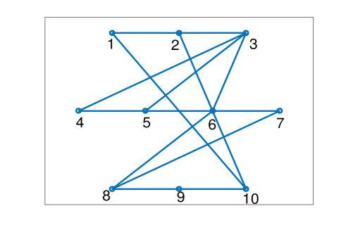
Figure 1: Graph Topology

Take a network of 10 agents interacting over a graph $\mathcal{G}$ to solve this problem. The information sharing graph $\mathcal{G}$ of the optimization algorithms is given in Fig. 1. Some simulation results using DPOFA algorithm (11) proposed in Section IV-A and DDFA algorithm (15) proposed in Section IV-B are shown in Figs. 2-6.

Figs. 2 and 3 show the trajectories of estimates for $x$ and the auxiliary variable $y$ versus time under DPOFA algorithm (11) proposed in Section IV-A, respectively, and Fig. 4 depicts the trajectories of the estimates for $x$ versus time under DDFA algorithm (15) proposed in Section IV-B. Algorithm (11) proposed in Section IV-A uses an auxiliary variable $y$ and estimates the optimal solution using $x=P_{\Omega}(y)$, while algorithm (15) proposed in Section IV-B directly uses $x$ to estimate the solution. Both algorithms are able to find the optimal solution of the optimization problem. Figs. 2-4 indicate that the trajectories of $y$ may be out of the constraint set $\Omega$, but the trajectories of $x$ stays in the constraint set $\Omega$.

Fig. 5 gives the trajectories of the objective function $f(x)$ and constraint $\|Wx-d_{0}\|^{2}$ versus time under DPOFA algorithm (11) and DDFA algorithm (15), and demonstrates that the trajectories of $x$ converge to the equality constraint. Furthermore, Fig. 6 verifies the boundedness of the trajectories of auxiliary variables $\lambda$ and $z$.

In Fig. 5, the trajectories of $f(x)$ and $\|Wx-d_{0}\|^{2}$ versus time under DPOFA algorithm show slow response speed at the beginning of the simulation. This is because the change of $y$ in the algorithm may not generate the changing behavior of $x=P_{\Omega}(y)$ when $y\notin\Omega$ (see the trajectories at the beginning of the simulation in Figs. 2 and 3). Due to the indirect feedback effect on $x$ (changing $x$ by controlling $y$) in DPOFA algorithm, the trajectory of variable $x$ may show slow changing behaviors in applications.

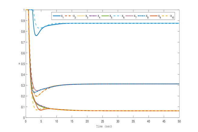
Figure 2: Trajectories of estimates for $x$ versus time under algorithm (11) for problem (38)

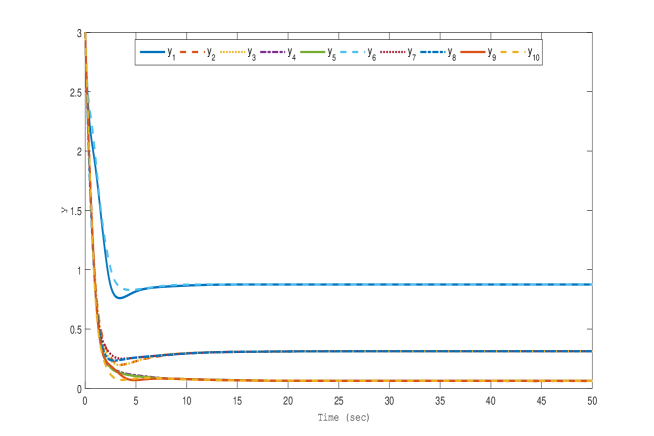
Figure 3: Trajectories of the auxiliary variable $y$ versus time under algorithm (11) for problem (38)

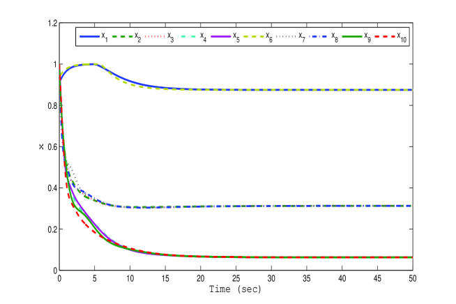
Figure 4: Trajectories of estimates for $x$ versus time under algorithm (15) for problem (38)

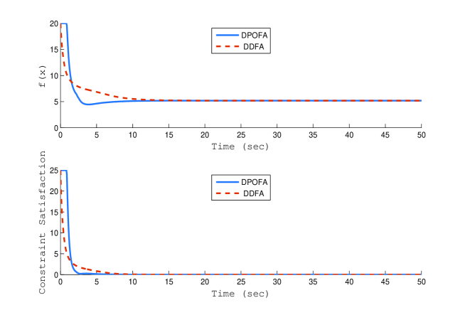
Figure 5: Objective functions $f(x)$ and constraints $\|Wx-d_{0}\|^{2}$ versus time under algorithms (11) and (15) for problem (38)

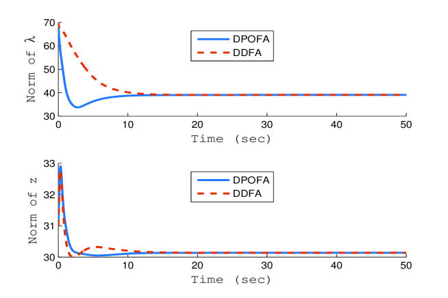
Figure 6: $\|\lambda\|^{2}$ and $\|z\|^{2}$ versus time under algorithms (11) and (15) for problem (38)

VI-B Multi-commodity Network Flow Problem

VI-B1 Problem Description

Consider a directed network consisting of a set $\mathcal{N}=\{1,\ldots,m\}$ of nodes and a set $\mathcal{E}$ of directed arcs. The flows on the arcs are of $S$ different types (commodities). The flows of the $s$th type on the arc $(i,j)$ is denoted by $t_{i,j}(s)\in[l_{i,j}(s),u_{i,j}(s)]$, where $[l_{i,j}(s),u_{i,j}(s)]$ is the capacity constraint for $t_{i,j}(s)$. The flows must satisfy the conservation of flow and supply/demand constraints of the form

$$\sum_{j|(i,j)\in\mathcal{E}}t_{i,j}(s)-\sum_{j|(j,i)\in\mathcal{E}}t_{j,i}(s)=b_{i}(s),$$ (39)

where $i\in\mathcal{N},\,s\in\{1,\ldots,S\},$ $b_{i}(s)$ is the amount of flow of the $s$th type entering the network at node $i$ ($b_{i}(s)>0$ indicates supply, and $b_{i}(s)<0$ indicates demand). The supplies/demands $b_{i}(s)$ are given and satisfy $\sum_{i\in\mathcal{N}}b_{i}(s)=0$ for the feasibility of the problem, which have been studied in the literature (see [18]).

The problem is to minimize $\sum_{(i,j)\in\mathcal{E}}f_{i,j}(t_{i,j}(1),\ldots,t_{i,j}(S))$ subject to the constraints (39), where $f_{i,j}:\mathbb{R}\rightarrow\mathbb{R}$ are continuous, strictly convex functions.

VI-B2 Reformulation of Problem

Let $n$ be the number of arcs in $\mathcal{E}$. We assign an index $k=k(i,j)\in\{1,\ldots,n\}$ to every arc $(i,j)\in\mathcal{E}$. We use $x_{k}=[t_{i,j}(1),\ldots,t_{i,j}(S)]^{\rm T}\in\mathbb{R}^{S}$ to denote the flow vector on arc $k$. Then constraint (39) can be rewritten as

$$A\otimes I_{S}x=\sum_{k=1}^{n}A_{k}\otimes I_{S}x_{k}=b,$$ (40)

with $A$ as the vertex-edge incidence matrix of the graph, $A_{k}$ as the $k$th column of $A$, $x=[x_{1}^{\rm T},\ldots,x_{n}^{\rm T}]^{\rm T}$, $b_{i}=[b_{i}(1),\ldots,b_{i}(S)]^{\rm T}$, and $b=[b_{1}^{\rm T},\ldots,b_{m}^{\rm T}]^{\rm T}$.

Let $f^{k}(x_{k})\triangleq f_{i,j}(t_{i,j}(1),\ldots,t_{i,j}(S))$, $\Omega_{k}=\prod_{s=1}^{S}[l_{i,j}(s),u_{i,j}(s)]$, where $k$ is the index of arc $(i,j)\in\mathcal{E}$. The optimization problem can be reformulated as

$$\min f(x)=\sum_{k=1}^{n}f^{k}(x_{k}),\quad\sum_{k=1}^{n}A_{k}\otimes I_{S}x_{k}=b,\quad x_{k}\in\Omega_{k},\quad k\in\{1,\ldots,n\}.$$ (41)

VI-B3 Numerical Simulation

Consider a network of 6 nodes and 12 arcs as shown in Fig. 7, with $S=1$. Let $f^{k}(x_{k})=\|x_{k}\|^{2}$, $x_{k}\in\mathbb{R}$ be the flows on arc $k$, and $\Omega_{k}=[0,10]$ for $k\in\{1,\ldots,12\}$. Problem (41) can be formulated as

$$\min\sum_{k=1}^{12}\|x_{k}\|^{2},\quad Ax=\sum_{k=1}^{12}A_{k}x_{k}=b,\quad x_{k}\in\Omega_{k},\quad k\in\{1,\ldots,12\},$$ (42)

where $b=[6,\,-7.2,\,-4.8,\,-9.6,\,8.4,\,7.2]^{\rm T}$ and $A_{k}$ is the $k$th column of the vertex-edge incidence matrix $A$ of the network in Fig. 7.

Simulation results using DPOFA algorithm (11) proposed in Section IV-A and DDFA algorithm (15) proposed in Section IV-B are shown in Figs. 8-12.

Fig. 8 shows the trajectories of estimates for $x$ versus time of DPOFA algorithm (11) proposed in Section IV-A, while Fig. 9 shows those of the auxiliary variables $y$ versus time of DPOFA algorithm (11) proposed in Section IV-A. Fig. 10 exhibits the trajectories of estimates for $x$ versus time of DDFA algorithm (15) proposed in Section IV-B. Algorithm (11) proposed in Section IV-A uses an auxiliary variable $y$ and estimates the optimal solution using $x=P_{\Omega}(y)$, while algorithm (15) proposed in Section IV-B directly uses $x$ to estimate the solution. Both algorithms are able to find the optimal solution of the optimization problem. Figs. 8-10 indicate that the trajectories of $y$ may be out of the constraint set $\Omega$, but the trajectories of $x$ stay in the constraint set $\Omega$.

Fig. 11 depicts the trajectories of the objective function $f(x)$ and constraint $\|Ax-b\|^{2}$ versus time under DPOFA algorithm (11) and DDFA algorithm (15), where the trajectories of $x$ converge to the equality constraint. Fig. 12 illustrates the boundedness of the trajectories of auxiliary variables $\lambda$ and $z$. Clearly, both algorithms can solve the problem.

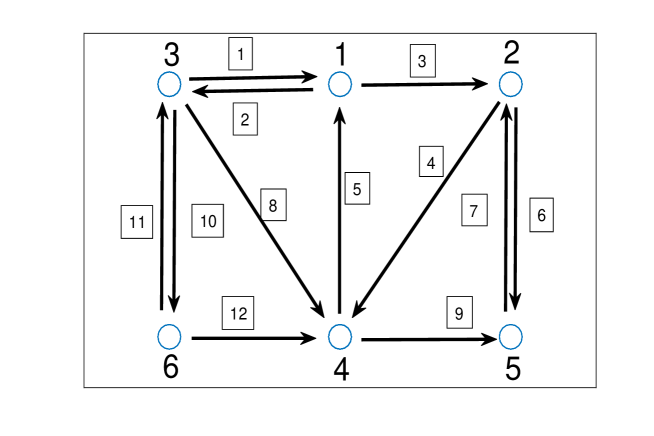
Figure 7: Graph Topology

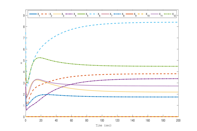
Figure 8: Trajectories of estimates for $x$ versus time under algorithm (11) for problem (42)

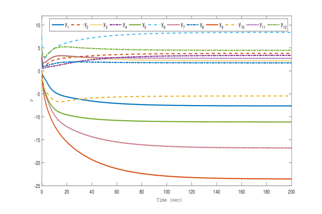
Figure 9: Trajectories of the auxiliary variable $y$ versus time under algorithm (11) for problem (42)

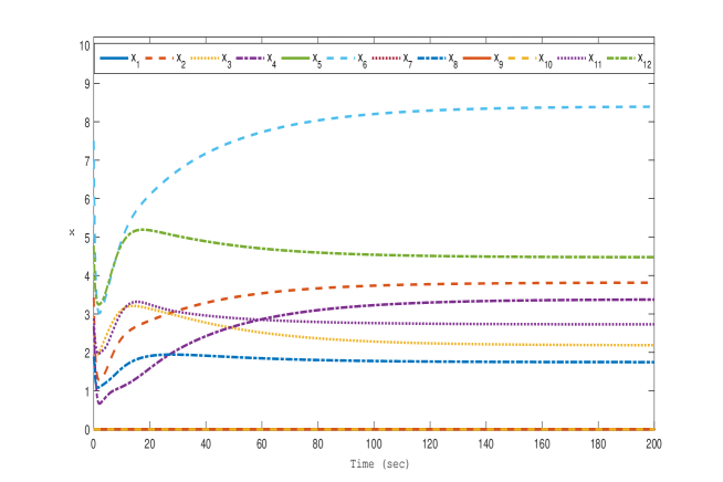
Figure 10: Trajectories of estimates for $x$ versus time under algorithm (15) for problem (42)

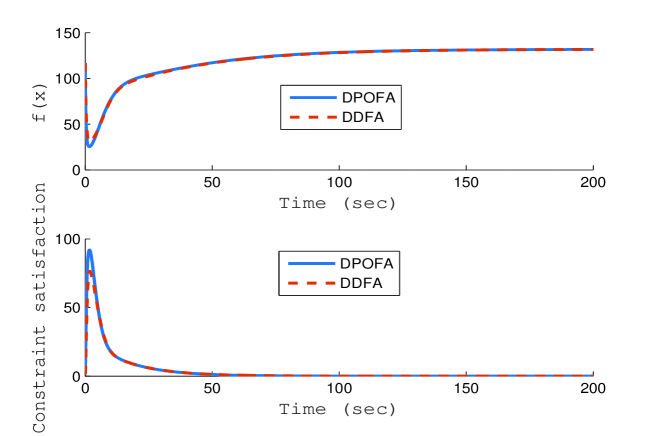
Figure 11: Objective functions $f(x)$ and constraints $\|Ax-b\|^{2}$ versus time under algorithms (11) and (15) for problem (42)

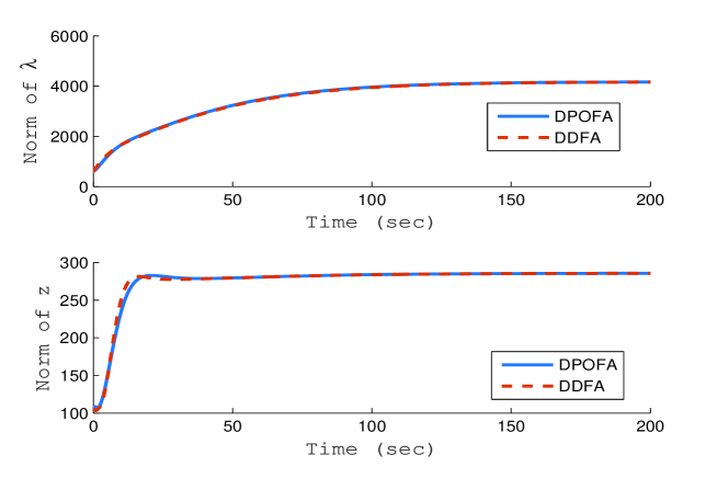
Figure 12: $\|\lambda\|^{2}$ and $\|z\|^{2}$ versus time under algorithms (11) and (15) for problem (42)

VII Conclusions

In this paper, the distributed design for the extended monotropic optimization (EMO) problem has been addressed, which is related to various applications in large-scale optimization and evolutionary computation. In this paper, two novel distributed continuous-time algorithms using projected output feedback design and derivative feedback design have been proposed to solve this problem in multi-agent networks. The design of the algorithms has used the decomposition of problem constraints and distributed techniques. Based on stability theory and invariance principle for differential inclusions, the convergence properties of the proposed algorithms have been established. The trajectories of all the agents have been proved to be bounded and convergent to the optimal solution with any initial condition in mathematical and numerical ways.

The distributed EMO problem definitely deserves more efforts because of its broad range of applications. In the future, distributed EMO problems with more complicated situations such as parameter uncertainties and online concerns will be further investigated.

References

- [1] Q. Liu and J. Wang, “A second-order multi-agent network for bound-constrained distributed optimization,” IEEE Transaction on Automatic Control, vol. 60, no. 12, pp. 3310–3315, 2015.
- [2] W. Bian and X. Xue, “Subgradient-based neural networks for nonsmooth nonconvex optimization problems,” IEEE Transactions on Neural Networks, vol. 20, no. 6, pp. 1024–1038, 2009.
- [3] P. Yi, Y. Hong, and F. Liu, “Distributed gradient algorithm for constrained optimization with application to load sharing in power systems,” Systems & Control Letters, vol. 83, pp. 45–52, 2015.
- [4] D. Yuan, D. W. C. Ho, and S. Xu, “Zeroth-order method for distributed optimization with approximate projections,” IEEE Transactions on Neural Networks and Learning Systems, vol. 27, no. 2, pp. 284–294, 2016.
- [5] A. Nedic, A. Ozdaglar, and P. A. Parrilo, “Constrained consensus and optimization in multi-agent networks,” IEEE Transactions on Automatic Control, vol. 55, pp. 922–938, 2010.
- [6] B. Gharesifard and J. Cortés, “Distributed continuous-time convex optimization on weight-balanced digraphs,” IEEE Transactions on Automatic Control, vol. 59, pp. 781–786, 2014.
- [7] G. Shi, K. Johansson, and Y. Hong, “Reaching an optimal consensus: Dynamical systems that compute intersections of convex sets,” IEEE Transactions on Automatic Control, vol. 55, no. 3, pp. 610–622, 2013.
- [8] Q. Liu, S. Yang, and J. Wang, “A collective neurodynamic approach to distributed constrained optimization,” IEEE Transactions on Neural Networks and Learning Systems, to appear.
- [9] D. Tank and J. Hopfield, “Simple neural optimization networks: An a/d converter, signal decision circuit, and a linear programming circuit,” IEEE Transactions on Circuits and Systems, vol. 33, no. 5, pp. 533–541, 2013.
- [10] E. Chong, S. Hui, and S. Zak, “An analysis of a class of neural networks for solving linear programming problems,” IEEE Transactions on Automatic Control, vol. 28, no. 3, pp. 36–73, 2008.
- [11] Q. Liu and J. Wang, “A one-layer projection neural network for nonsmooth optimization subject to linear equalities and bound constraints,” IEEE Transactions on Neural Networks and Learning Systems, vol. 24, no. 5, pp. 812–824, 2013.
- [12] J. Park, K. Lee, J. Shin, and K. Y. Lee, “Economic load dispatch for non-smooth cost functions using particle swarm optimization,” in IEEE Power Engineering Society 2003 General Meeting, Toronto, Canada, 2003, pp. 938–943.
- [13] E. Ramírez-Llanos and S. Martínez, “Distributed and robust resource allocation algorithms for multi-agent systems via discrete-time iterations,” in Proc. IEEE Conf. Decision Control, Osaka, Japan, 2015, pp. 1390–1396.
- [14] P. Yi, Y. Hong, and F. Liu, “Initialization-free distributed algorithms for optimal resource allocation with feasibility constraints and its application to economic dispatch of power systems,” arXiv:1510.08579, 2015.
- [15] P. N. M. Forti and M. Quincampoix, “Generalized neural network for nonsmooth nonlinear programming problems,” IEEE Transactions on Circuits and Systems-I, vol. 51, no. 9, pp. 1741–1754, 2004.
- [16] R. Rockafellar, Network Flows and Monotropic Optimization. New York: Wiley, 1984.
- [17] ——, “Monotropic programming: A generalization of linear programming and network programming. in: Convexity and duality in optimization,” Lecture Notes in Economics and Mathematical Systems, vol. 256, pp. 226–237, 1985.
- [18] D. P. Bertsekas, “Extended monotropic programming and duality,” Journal of Optimization Theory and Applications, vol. 139, no. 2, pp. 209–225, 2008.
- [19] N. Chatzipanagiotis, D. Dentcheva, and M. M. Zavlanos, “An augmented lagrangian method for distributed optimization,” Mathematical Programming Series A, vol. 152, no. 1, pp. 405–434, 2015.
- [20] C. Godsil and G. F. Royle, Algebraic Graph Theory. New York: Springer-Verlag, 2001.
- [21] J. P. Aubin and A. Cellina, Differential Inclusions. Berlin, Germany: Springer-Verlag, 1984.
- [22] F. H. Clarke, Optimization and Nonsmooth Analysis. New York: Wiley, 1983.
- [23] A. Bacciotti and F. Ceragioli, “Stability and stabilization of discontinuous systems and nonsmooth Lyapunov functions,” ESAIM: Control, Optimisation and Calculus of Variations, vol. 4, pp. 361–376, 1999.
- [24] J. Cortés, “Discontinuous dynamical systems,” IEEE Control Systems Magazine, vol. 44, no. 11, pp. 1995–2006, 1999.
- [25] Z. Denkowski, S. Migórski, and N. S. Papageorgiou, An Introduction to Nonlinear Analysis: Theory. New York, NY: Springer-Verlag New York Inc., 2003.
- [26] D. Kinderlehrer and G. Stampacchia, An Introduction to Variational Inequalities and Their Applications. New York: Academic, 1982.
- [27] Z. Qiu, S. Liu, and L. Xie, “Distributed constrained optimal consensus of multi-agent systems,” Automatica, vol. 68, pp. 209–215, 2016.
- [28] M. Tygert, “A fast algorithm for computing minimal-norm solutions to underdetermined systems of linear equations,” arXiv:0905.4745, 2009.
- [29] S. Mou, J. Liu, and A. S. Morse, “A distributed algorithm for solving a linear algebraic equation,” IEEE Transactions on Automatic Control, vol. 60, no. 11, pp. 2863–2878, 2015.
- [30] A. Ruszczynski, Nonlinear Optimization. Princeton, New Jersey: Princeton University Press, 2006.
- [31] A. Cherukuri and J. Cortés, “Distributed generator coordination for initialization and anytime optimization in economic dispatch,” IEEE Transactions on Control of Network Systems, vol. 2, no. 3, pp. 226–237, 2015.
- [32] G. Strang, “The fundamental theorem of linear algebra,” American Mathematical Monthly, vol. 100, no. 9, pp. 848–855, 1993.
- [33] W. M. Haddad and V. Chellaboina, Nonlinear Dynamical Systems and Control: A Lyapunov-Based Approach. Princeton, NJ: Princeton Univ. Press, 2008.