Classification of scaling limits of uniform quadrangulations with a boundary

Abstract

We study non-compact scaling limits of uniform random planar quadrangulations with a boundary when their size tends to infinity. Depending on the asymptotic behavior of the boundary size and the choice of the scaling factor, we observe different limiting metric spaces. Among well-known objects like the Brownian plane or the infinite continuum random tree, we construct two new one-parameter families of metric spaces that appear as scaling limits: the Brownian half-plane with skewness parameter $\theta$ and the infinite-volume Brownian disk of perimeter $\sigma$. We also obtain various coupling and limit results clarifying the relation between these objects.

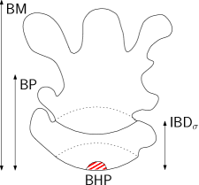
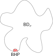
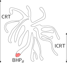
Figure 1: Schematic representation of the non-trivial scaling limits in the regimes $1\ll\sigma_{n}\ll\sqrt{n}$ (left), $\sigma_{n}\approx\sqrt{n}$ (middle), $\sqrt{n}\ll\sigma_{n}\ll n$ (right). See the listings in Section 1.1.

1 Introduction

In this work, we obtain a complete classification of possible scaling limits of finite random planar quadrangulations with a boundary when their size tends to infinity.

Recall that a planar map is a proper embedding of a finite connected graph in the two-dimensional sphere. The graph may have loops and multiple edges. The faces of a map are the connected components of the complement of its edges. A planar quadrangulation with a boundary is a particular planar map where its faces have degree four, i.e., are incident to four oriented edges (an edge is counted twice if it lies entirely in the face), except possibly one face which may have an arbitrary (even) degree. This face is referred to as the external face, where the other faces that form quadrangles are called internal faces. The boundary of the map is given by the oriented edges that are incident to the external face, and the number of such edges is called the size of the boundary, or the perimeter of the map. The size of the map is given by the number of internal faces. We do not ask for the boundary to be a simple curve. We always consider rooted maps with a boundary, which means that we distinguish one oriented edge of the boundary such that the root face lies to the left of that edge. This edge will be called the root edge, and its origin the root vertex. As usual, two (rooted) maps are considered equivalent if they differ by an orientation- and root-preserving homeomorphism of the sphere.

We are interested in scaling limits of planar maps picked uniformly at random among all quadrangulations with a boundary when the size and (possibly) the perimeter of the map tend to infinity. This means that we view the vertex set of the quadrangulation as a metric space for the graph distance and consider (under a suitable rescaling of the distance) distributional limits of such metric spaces, either in the global or local Gromov-Hausdorff topology.

In [29] and independently in [33], it was shown that uniformly chosen quadrangulations of size $n$, equipped with the graph distance $d_{\textup{gr}}$ rescaled by a factor $n^{-1/4}$, converge to a random compact metric space called the Brownian map. The latter turns out to be a universal object which appears as the distributional limit of many classes of random maps. We refer to the recent overview [34] for various aspect of the Brownian map and for more references.

Here we shall deal with quadrangulations of size $n$ having a boundary of size $2\sigma_{n}$, and we will distinguish three boundary regimes as $n$ tends to infinity:

$${\bf a})\,\,\sigma_{n}/\sqrt{n}\rightarrow 0;\quad{\bf b})\,\,\sigma_{n}/\sqrt{n}\rightarrow\sqrt{2}\sigma\;\hbox{ for some }\sigma\in(0,\infty);\quad{\bf c})\,\,\sigma_{n}/\sqrt{n}\rightarrow\infty.$$

Bettinelli [7] showed that in regime a), the boundary becomes negligible in the scale $n^{-1/4}$, and the Brownian map appears in the limit when $n$ tends to infinity. In regime b), he obtained under the same rescaling convergence along appropriate infinite subsequences to a random metric space called the Brownian disk $\textup{{BD}}_{\sigma}$. Uniqueness of this limit was later established by Bettinelli and Miermont in [9]. For the third regime c), it is shown in [7] that a rescaling by $\sigma_{n}^{-1/2}$ leads in the limit to Aldous’s continuum random tree CRT [1, 2].

The scaling factors considered by Bettinelli [7] ensure that the diameter of the rescaled planar map stays bounded in probability. Consequently, the limits he obtains are random compact metric spaces, and the right notion of convergence is the Gromov-Hausdorff convergence in the space of (isometry classes of) compact metric spaces.

We will study all possible scalings $a_{n}\rightarrow\infty$ in all the above boundary regimes. When $a_{n}$ grows slower then the diameter of the map as $n$ tends to infinity, the right notion of convergence is the local Gromov-Hausdorff convergence. Depending on the ratio of perimeter and scaling parameter, the boundary will in the limit be either invisible, or of a size comparable to the full map, or dominate the map.

In the process we obtain two new one-parameter families of limit spaces: the Brownian half-plane $\textup{{BHP}}_{\theta}$ with parameter $\theta\in[0,\infty)$ and the infinite-volume Brownian disk $\textup{{IBD}}_{\sigma}$ with boundary length $\sigma\in(0,\infty)$.

The Brownian disk $\textup{{BD}}_{\sigma}$ and the Brownian half-plane $\textup{{BHP}}=\textup{{BHP}}_{0}$ play a central role in this work. The latter can be seen as the Gromov-Hausdorff tangent cone in distribution of $\textup{{BD}}_{\sigma}$ at its root, and also as the scaling limit of the so-called uniform infinite half-planar quadrangulation UIHPQ, which in turn arises as the local limit in the sense of Benjamini and Schramm of uniform quadrangulations with $n$ faces and a boundary growing slower than $n$.

The space $\textup{{BHP}}_{\theta}$ for $\theta>0$ can be understood as an interpolation between BHP (when $\theta\to 0$) and the so-called infinite continuum random tree ICRT introduced by Aldous [1] (when $\theta\to\infty$). The $\textup{{IBD}}_{\sigma}$ in turn interpolates between BHP (when $\sigma\rightarrow\infty$) and the Brownian plane BP introduced by Curien and Le Gall [19, 20] (when $\sigma\rightarrow 0$). See also the recent work of Budzinski [14] for a hyperbolic version of the Brownian plane. These interpretations are easy consequences of our results. We refer to Remark 3.19 and the exercises there for the exact statements.

For a better overview, we begin with a rough list of our main results on scaling limits of finite-size quadrangulations with a boundary (including results of [7] and [9]). We then mention further results that will be obtained below, including limit statements on $\textup{{BD}}_{\sigma}$. The precise formulations can be found in Section 3, after a proper definition of the limit spaces and a reminder on the notion of convergence in Section 2.

As in many works in this context, our approach is based on the Bouttier-Di Francesco-Guitter bijection [13, 12], which establishes a one-to-one correspondence between (finite-size) quadrangulations with a boundary on the one hand and discrete labeled forests and bridges on the other hand. The bijection is recalled in Section 4. Section 5 contains some more auxiliary results, mostly convergence results on forests and bridges when their size tends to infinity. The statements proved there are of some independent interest, but can also be skipped at first reading. Section 6 contains all the proofs of our main statements.

1.1 Overview over the main results

For any $\sigma_{n}\in\mathbb{N}=\{1,2,\ldots\}$, we write $Q_{n}^{\sigma_{n}}$ for a uniformly distributed rooted quadrangulation with $n$ inner faces and a boundary of size $2\sigma_{n}$. The vertex set of $Q_{n}^{\sigma_{n}}$ is denoted by $V(Q_{n}^{\sigma_{n}})$, $\rho_{n}$ represents the root vertex and $d_{\textup{gr}}$ stands for the graph distance on $V(Q_{n}^{\sigma_{n}})$. For any two sequences $(a_{n},n\in\mathbb{N}),(b_{n},n\in\mathbb{N})$ of reals, we write $a_{n}\ll b_{n}$ or $b_{n}\gg a_{n}$ if and only if $a_{n}/b_{n}\to 0$ as $n\to\infty$, and we write $a_{n}\sim b_{n}$ if $a_{n}/b_{n}\to 1$.

We denote by $\circ$ the trivial one-point metric space and write s-Lim ($\textsf{s-Lim}_{\textup{loc}}$) for the distributional scaling limit of $(V(Q_{n}^{\sigma_{n}}),a_{n}^{-1}d_{\textup{gr}},\rho_{n})$ in the Gromov-Hausdorff topology (in the local Gromov-Hausdorff topology) as $n$ tends to infinity.

The regime $\sigma_{n}\ll\sqrt{n}$.

• If $1\ll a_{n}\ll\sqrt{\sigma_{n}}$, then $\textup{$\textsf{s-Lim}_{\textup{loc}}$}=\textup{{BHP}}.$ • If $1\ll a_{n}\sim(1/9)^{1/4}\sqrt{2\sigma_{n}/\sigma}$, $\sigma\in(0,\infty)$, then $\textup{$\textsf{s-Lim}_{\textup{loc}}$}=\textup{{IBD}}_{\sigma}.$ • If $\sqrt{\sigma_{n}}\ll a_{n}\ll n^{1/4}$, then $\textup{$\textsf{s-Lim}_{\textup{loc}}$}=\textup{{BP}}.$ • If $a_{n}\sim(8/9)^{1/4}n^{1/4}$, then (see [7]) $\textup{$\textsf{s-Lim}$}=\textup{{BM}}.$ • If $a_{n}\gg n^{1/4}$, then $\textup{$\textsf{s-Lim}$}=\circ\,.$

The regime $\sigma_{n}\sim\sigma\sqrt{2n}$, $\sigma\in(0,\infty)$.

• If $1\ll a_{n}\ll n^{1/4}$, then $\textup{$\textsf{s-Lim}_{\textup{loc}}$}=\textup{{BHP}}.$ • If $a_{n}\sim(8/9)^{1/4}n^{1/4}$, then (see [7] and [9]) $\textup{$\textsf{s-Lim}$}=\textup{{BD}}_{\sigma}.$ • If $a_{n}\gg n^{1/4}$, then $\textup{$\textsf{s-Lim}$}=\circ\,.$

The regime $\sigma_{n}\gg\sqrt{n}$.

• If $\sigma_{n}\ll n$ and $\lim_{n\rightarrow\infty}(9/4)^{1/4}a_{n}/\sqrt{2n/\sigma_{n}}=\sqrt{\theta}\in[0,\infty)$, then $\textup{$\textsf{s-Lim}_{\textup{loc}}$}=\textup{{BHP}}_{\theta}.$ • If $\max\{1,\sqrt{n/\sigma_{n}}\}\ll a_{n}\ll\sqrt{\sigma_{n}}$, then $\textup{$\textsf{s-Lim}_{\textup{loc}}$}=\textup{{ICRT}}.$ • If $a_{n}\sim\sqrt{2\sigma_{n}}$ (see [7]), then $\textup{$\textsf{s-Lim}$}=\textup{{CRT}}.$ • If $a_{n}\gg\sqrt{\sigma_{n}}$, then $\textup{$\textsf{s-Lim}$}=\circ\,.$

The new results in these listings are covered by Theorems 3.1, 3.2, 3.3, 3.4 and 3.5 below.

In the regime $\sigma_{n}\ll\sqrt{n}$ in the first list, the last three convergences include the case of bounded $\sigma_{n}$. In the last regime $\sigma_{n}\gg\sqrt{n}$, we allow $\sigma_{n}$ to grow faster than $n$. The scaling constants are chosen in such a way that the description of the limiting objects is the most natural. See also Figure 1 for a schematic representation.

Figure 2 shows all possible regimes in one diagram, in which the $x$-axis denotes the limiting possible values for the logarithm of the boundary length $\log(\sigma_{n})/\log(n)$ in units of $\log(n)$, and the $y$-axis corresponds to the limit of the logarithm of the scaling factor $\log(a_{n})/\log(n)$ in units of $\log(n)$. For the specific value $y=0$, it will be assumed that $a_{n}=1$, so that we are really in the regime of local limits, without any rescaling. Similarly, for some specific values of $(x,y)$, that are shown on the colored lines, we will require some particular scaling behaviors that are detailed in the list above. For instance, for $x=1/2$ and $y=1/4$, we really ask that $\sigma_{n}\sim\sigma\sqrt{2n}$ for some $\sigma>0$ and $a_{n}\sim(8/9)^{1/4}n^{1/4}$.

As it is shown in Theorem 3.6, the BHP can also be obtained from the UIHPQ by zooming-out around the root: $\lambda\cdot\textup{{UIHPQ}}\rightarrow\textup{{BHP}}$ in distribution in the local Gromov-Hausdorff sense as $\lambda\to 0$. Here, $\lambda\cdot\textup{{UIHPQ}}$ is obtained from UIHPQ by keeping the same set of points, but rescaling the metric by a factor $\lambda$, see Section 2.4.2 below.

Many of our results, for example those involving the Brownian half-planes $\textup{{BHP}}_{\theta}$, $\theta\geq 0$, are based on coupling methods, which yield in fact stronger statements than those mentioned above. In particular, couplings will allow us to deduce that the topology of $\textup{{BHP}}_{\theta}$ is that of a closed half-plane, whereas $\textup{{IBD}}_{\sigma}$ is homeomorphic to the pointed closed disk (Corollaries 3.8 and 3.13).

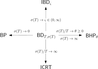
Figure 5: Zooming-in around the root of the Brownian disk $\textup{{BD}}_{T,\sigma(T)}$ of volume $T$ and perimeter $\sigma(T)$. The figure shows all possible weak limits in the local Gromov-Hausdorff sense when $T\rightarrow\infty$ (Corollaries 3.15, 3.16, 3.17, 3.18).

The above results will moreover enable us to determine the limiting behavior of the Brownian disk $\textup{{BD}}_{T,\sigma}$ of volume $T$ and perimeter $\sigma$ when zooming-in around its root vertex, or, equivalently by scaling, by blowing up its volume and perimeter. Depending on the behavior of the “perimeter” function $\sigma(\cdot):(0,\infty)\rightarrow(0,\infty)$ for large volumes $T$, we observe BP, $\textup{{IBD}}_{\varsigma}$, $\textup{{BHP}}_{\theta}$ or the ICRT as the distributional limit in the local Gromov-Hausdorff sense of $\textup{{BD}}_{T,\sigma(T)}$ when $T\rightarrow\infty$. See Figure 5 below and Corollaries 3.15, 3.16, 3.17, 3.18.

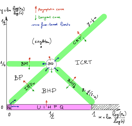
Figure 2: The user’s manual to this paper, displaying all possible regimes and limits for the rescaled pointed space $(V(Q_{n}^{\sigma_{n}}),a_{n}^{-1}d_{\textup{gr}},\rho_{n})$.

2 Definitions

In this section, we define our limit objects and recall some facts about the (local) Gromov-Hausdorff convergence and the local limits of maps.

All our limit metric spaces will be defined in terms of certain random processes. To make the presentation unified, we will denote by $(X,W)$ the canonical continuous process in $\mathcal{C}(I,\mathbb{R})^{2}$, where $I$ will be an interval of the form $I=[0,T]$ for some $T>0$, or $I=\mathbb{R}$. The set $\mathcal{C}(I,\mathbb{R})$ of continuous functions on $I$ is equipped with the compact-open topology (topology of uniform convergence over compact subsets of $I$).

For $t\in I\cap[0,\infty)$, we write $\underline{X}_{t}=\inf_{[0,t]}X,$ and in case $I=\mathbb{R}$, we put for $t<0$ $\underline{X}_{t}=\inf_{(-\infty,t]}X.$

If $Y=(Y_{t}:t\geq 0)$ is a real-valued process indexed by the positive real half-line, we write $\Pi(Y)$ for its Pitman transform defined as $\Pi(Y)_{t}=Y_{t}-2\underline{Y}_{t}$, $t\geq 0$. We will often use the fact that if $B=(B_{t},t\geq 0)$ is a standard Brownian motion, then its Pitman transform $\Pi(B)$ has the law of a three-dimensional Bessel process, and $\inf_{[t,\infty)}\Pi(B)=-\inf_{[0,t]}B$ for every $t\geq 0$. See [36, Theorem 0.1 (ii)].

2.1 Metric spaces coded by real functions

Real trees.

If $f$ is an element of $\mathcal{C}(I,\mathbb{R})$, and $s,t\in I$, we denote by $\underline{f}(s,t)$ the quantity

$$\underline{f}(s,t)=\left\{\begin{array}[]{lcl}\inf_{[s,t]}f&\mbox{ if }&s\leq t\\ \inf_{I\setminus[t,s]}f&\mbox{ if }&s>t\end{array}\right.,$$

and for $s,t\in I$ we let

$$d_{f}(s,t)=f(s)+f(t)-2\max(\underline{f}(s,t),\underline{f}(t,s))\,.$$

This defines a pseudo-metric on $I$, which is a class function for the equivalence relation $\{d_{f}=0\}$. Therefore, we can define the quotient space $\mathcal{T}_{f}=I/\{d_{f}=0\}$, on which $d_{f}$ induces a true distance, still denoted by $d_{f}$ for simplicity. Since we assumed that $I$ contains $0$, it is natural to “root” the space $(\mathcal{T}_{f},d_{f})$ at the point $\rho$ given by the equivalence class $[0]=\{s\in I:d_{f}(0,s)=0\}$ of $0$.

The metric space $(\mathcal{T}_{f},d_{f},\rho)$ is called the continuum tree coded by $f$. In more precise terms, it is a rooted $\mathbb{R}$-tree, which is also compact if $I$ is compact. This fact is well-known in the “classical case” where $f$ is a non-negative function on an interval $[0,T]$, and $f(0)=f(T)=0$, see, e.g. [30, Section 3], but it remains true in this more general context. This fact will not be used in this paper, so we do not prove it here.

Note that the space $(\mathcal{T}_{f},d_{f})$ comes with a natural Borel $\sigma$-finite measure, $\mu_{f}$, which is defined as the push-forward of the Lebesgue measure on $I$ by the canonical projection $p_{f}:I\to\mathcal{T}_{f}$.

Metric gluing of a real tree on another.

Let $f,g$ be two elements of $\mathcal{C}(I,\mathbb{R})$. These functions code two $\mathbb{R}$-trees $\mathcal{T}_{f},\mathcal{T}_{g}$ in the preceding sense. We now define a new metric space $(M_{f,g},D_{f,g})$ by informally quotienting the space $(\mathcal{T}_{g},d_{g})$ by the equivalence relation $\{d_{f}=0\}$. Formally, for $s,t\in I$, we let

$$D_{f,g}(s,t)=\inf\left\{\sum_{i=1}^{k}d_{g}(s_{i},t_{i}):\begin{array}[]{l}k\geq 1,\,s_{1},\ldots,s_{k},t_{1},\ldots,t_{k}\in I,s_{1}=s,t_{k}=t,\\ d_{f}(t_{i},s_{i+1})=0\mbox{ for every }i\in\{1,2,\ldots,k-1\}\end{array}\right\}\,.$$ (2.1)

This defines a pseudo-metric on $I$, and we let $M_{f,g}$ be the quotient space $I/\{D_{f,g}=0\}$, endowed with the true metric inherited from $D_{f,g}$ (and again, still denoted by $D_{f,g}$). Again, this space is naturally pointed at the equivalence class of $0$ for $\{D_{f,g}=0\}$, which we still denote by $\rho$.

Again, the space $(M_{f,g},D_{f,g})$ is naturally endowed with the measure $\mu_{f,g}$, defined as the push-forward of the Lebesgue measure on $I$ by the canonical projection $p_{f,g}:I\to M_{f,g}$.

2.2 Random snakes

The definition for most of our limiting random spaces depend on the notion of a random snake, which we now introduce. Let $f\in\mathcal{C}(I,\mathbb{R})$ be a continuous path on an interval $I$. The random snake driven by $f$ is a random Gaussian process $(Z^{f}_{s},s\in I)$ satisfying $Z^{f}_{0}=0$ a.s. and

$$\mathbb{E}[|Z^{f}_{s}-Z^{f}_{t}|^{2}]=d_{f}(s,t)\,.$$

These specifications characterize the law of $Z^{f}$: roughly speaking, it can be seen as Brownian motion indexed by the tree $\mathcal{T}_{f}$, see, e.g., Section 4 of [30]. It is easy to see and well-known that the process $Z^{f}$ admits a continuous modification as soon as $f$ is a locally Hölder-continuous function on $I$. In this case, we always work with this modification.

The snake driven by a random function $Y$ is then defined as the random Gaussian process $Z^{Y}$ conditionally given $Y$. In all our applications, $Y$ will be considered under probability distributions that make it a Hölder-continuous function with probability one.

More specifically, except for the case of the infinite-volume Brownian disk, see below, we will either let $Y=X$ for $X$ the canonical process on $\mathcal{C}(I,\mathbb{R})$ (namely for the Brownian map and the Brownian plane), or $Y=X-\underline{X}$ (for the Brownian disk and the Brownian half-planes).

2.3 Limit random metric spaces

We apply the preceding constructions to a variety of random versions of the functions $f,g$.

2.3.1 Compact spaces

In this section the processes considered all take values in $\mathcal{C}([0,T],\mathbb{R})$ for some $T>0$.

Continuum random tree $\textup{{CRT}}_{T}$, $T>0$.

The continuum random tree was introduced by Aldous [1, 2] and is defined as follows.

Definition 2.1.

Let $T>0$. The continuum random tree $\textup{{CRT}}_{T}$ with volume $T$ is the random rooted real tree $(\mathcal{T}_{X},d_{x},\rho)$ for the probability distribution that makes the canonical process $X$ of $\mathcal{C}([0,T],\mathbb{R})$ the standard Brownian excursion with duration $T$.

The term “CRT” usually denotes $\textup{{CRT}}_{1}$ with volume $T=1$, in which case $X$ is taken under the law of the normalized Brownian excursion. We simply write CRT instead of $\textup{{CRT}}_{1}$.

Note the scaling relation, for $\lambda,T>0$:

$$\lambda\cdot\textup{{CRT}}_{T}=_{d}\textup{{CRT}}_{\lambda^{2}T}\,.$$

This comes from the fact that, if $\mathbbm{e}^{T}$ is a Brownian excursion with duration $T$, then $\lambda\mathbbm{e}^{T}(\cdot/\lambda^{2})$ has same distribution as $\mathbbm{e}^{\lambda^{2}T}$.

We should also discuss the role of $\rho$ in the above definition. The re-rooting property of $\textup{{CRT}}_{T}$ [2, (20)] states, roughly speaking, that if $\rho^{\prime}$ is a random variable with distribution $\mu_{X}/\mu_{X}(1)$ (the normalized version of the measure defined above), then $(\mathcal{T}_{X},d_{X},\rho^{\prime})$ has same distribution as $(\mathcal{T}_{X},d_{X},\rho)$. In this sense, the point $\rho$ plays no distinguished role in the construction of $\textup{{CRT}}_{T}$.

Brownian map $\textup{{BM}}_{T}$, $T>0$.

The Brownian map is roughly speaking the metric gluing of the tree coded by a snake driven by a normalized Brownian excursion, on the tree coded by the excursion itself.

Definition 2.2.

The Brownian map $\textup{{BM}}_{T}$ with volume $T$ is the metric space $(M_{X,W},D_{X,W},\rho)$ for the probability law that makes $X$ a Brownian excursion of duration $T$, and $W$ is the snake driven by $X$.

We write BM instead of $\textup{{BM}}_{1}$. The scaling properties of Gaussian processes imply easily that for $\lambda>0$,

$$\lambda\cdot\textup{{BM}}_{T}=_{d}\textup{{BM}}_{\lambda^{4}T}\,.$$

Just as for $\textup{{CRT}}_{T}$, the point $\rho$ in $\textup{{BM}}_{T}$ should be seen as a random choice according to the normalized measure $\mu_{X,W}/\mu_{X,W}(1)$, which is known as the re-rooting property of the Brownian map (Theorem 8.1 of [28]). The latter is a crucial property for characterizing the Brownian map, see, e.g., the recent work [35].

Brownian disk $\textup{{BD}}_{T,\sigma}$, $\sigma\in(0,\infty)$, $T>0$.

The Brownian disk first appears in [7] as limiting metric space along suitable infinite subsequences. Uniqueness of the limit and a concrete description of the metric were obtained in [9].

The description is slightly more elaborate than that of the Brownian map. For $t\geq 0$, we let $\underline{X}_{t}=\inf_{[0,t]}X$.

Definition 2.3.

The Brownian disk $\textup{{BD}}_{T,\sigma}$ with volume $T$ and boundary length $\sigma$ is the metric space $(M_{X,W},D_{X,W},\rho)$ under the probability measures that makes $X$ a first-passage Brownian bridge from $0$ to $-\sigma$ of duration $T$, and conditionally given $X$, $(W_{t},0\leq t\leq T)$ has same distribution as $(\sqrt{3}\,\gamma_{-\underline{X}_{t}}+Z_{t},0\leq t\leq T)$, where

• $(Z_{t},0\leq t\leq T)=Z^{X-\underline{X}}$ is the random snake driven by the reflected process $(X_{t}-\underline{X}_{t},0\leq t\leq T)$, i.e., (a continuous modification of) the centered Gaussian process with covariances given by

  $$\mathbb{E}\left[Z_{s}Z_{t}\right]=\min_{[s\wedge t,s\vee t]}(X-\underline{X}).$$

• $(\gamma_{x},0\leq x\leq\sigma)$ is a standard Brownian bridge with duration $\sigma$, independent of $Z^{X-\underline{X}}$.

The Brownian disks are homeomorphic to the closed unit disk $\overline{\mathbb{D}}$, where $\mathbb{D}=\{z\in\mathbb{C}:|z|<1\}$, see [7, Proposition 21] (cited as Lemma 6.12 below). They enjoy the following scaling property: For $\lambda>0$,

$$\lambda\cdot\textup{{BD}}_{T,\sigma}=_{d}\textup{{BD}}_{\lambda^{4}T,\lambda^{2}\sigma}\,.$$

If $T=1$, we will simply write $\textup{{BD}}_{\sigma}$ instead of $\textup{{BD}}_{1,\sigma}$. Contrary to the Brownian tree or the Brownian map, $\rho$ does not play the role of a random point distributed according to $\mu_{X,W}/\mu_{X,W}(1)$. The reason is that $\rho$ is a.s. a point of the boundary of the disk, which is of zero measure, see [9] for more details.

2.3.2 Non-compact spaces

In this subsection, all processes take values in $\mathcal{C}(\mathbb{R},\mathbb{R})$.

Infinite continuum random tree ICRT.

The ICRT is process $2$ in [1] and can be defined as follows.

Definition 2.4.

The infinite continuum random tree ICRT is the random rooted real tree $(\mathcal{T}_{X},d_{X},\rho)$, for the probability distribution under which the canonical process $X$ in $\mathcal{C}(\mathbb{R},\mathbb{R})$ is such that $(X_{t},t\geq 0)$ and $(X_{-t},t\geq 0)$ are two independent standard three-dimensional Bessel processes started at $0$.

This results in an a.s. non-compact real tree, which enjoys the remarkable self-similarity property that $\lambda\cdot\textup{{ICRT}}=_{d}\textup{{ICRT}}$ for every $\lambda>0$.

Note that if we let $Y$ be the canonical process in $\mathcal{C}(\mathbb{R},\mathbb{R})$ such that $(Y_{t},t\geq 0)$ and $(Y_{-t},t\geq 0)$ are two independent standard Brownian motions, then the random rooted real tree $(\mathcal{T}_{Y},d_{Y},[0])$ has same distribution as ICRT. This follows readily from the fact that $\Pi((Y_{t},t\geq 0))$ has the law of a three-dimensional Bessel process.

Brownian plane BP.

The Brownian plane was introduced in [19].

Definition 2.5.

The Brownian plane BP is the pointed space $(M_{X,W},D_{X,W},\rho)$ under the probability distribution such that

• $(X_{t},t\geq 0)$ and $(X_{-t},t\geq 0)$ are two independent three-dimensional Bessel processes.

• Given $X=(X_{t},t\in\mathbb{R})$, $W$ has same distribution as the random snake $Z^{X}$ driven by $X$.

The Brownian plane is a.s. homeomorphic to $\mathbb{R}^{2}$, and is invariant under scaling: for $\lambda>0$,

$$\lambda\cdot\textup{{BP}}=_{d}\textup{{BP}}\,.$$

Brownian half-planes $\textup{{BHP}}_{\theta}$, $\theta\in[0,\infty)$.

The Brownian half-planes are the first truly new limiting metric spaces that we encounter in this study. Recall that $\underline{X}_{t}=\inf_{[0,t]}X$ for $t\geq 0$ and $\underline{X}_{t}=\inf_{(-\infty,t]}X$ for $t<0$.

Definition 2.6.

Let $\theta\geq 0$ be fixed. The Brownian half-plane $\textup{{BHP}}_{\theta}$ with skewness parameter $\theta$ is the pointed space $(M_{X,W},D_{X,W},\rho)$ under the probability distribution such that

• $(X_{t},t\geq 0)$ is a standard Brownian motion with linear drift $-\theta$, and $(X_{-t},t\geq 0)$ is the Pitman transform $\Pi(X^{\prime})$ of an independent copy $X^{\prime}$ of $(X_{t},t\geq 0)$.

• Given $X$, $W$ has same distribution as $(\sqrt{3}\,\gamma_{-\underline{X}_{t}}+Z_{t},t\in\mathbb{R})$, where

  • $(Z_{t},t\in\mathbb{R})=Z^{X-\underline{X}}$ is the snake driven by the process $(X_{t}-\underline{X}_{t},t\in\mathbb{R})$, i.e., the centered Gaussian process with covariances given by

    $$\mathbb{E}\left[Z_{s}Z_{t}\right]=\min_{[s\wedge t,s\vee t]}(X-\underline{X}).$$

  • $(\gamma_{x},x\in\mathbb{R})$ is a two-sided standard Brownian motion with $\gamma_{0}=0$, independent of $Z^{X-\underline{X}}$.

The scaling property enjoyed by $\textup{{BHP}}_{\theta}$ is that for $\lambda>0$,

$$\lambda\cdot\textup{{BHP}}_{\theta}=_{d}\textup{{BHP}}_{\theta/\lambda^{2}}\,.$$

This makes the value $\theta=0$ special in the sense that the space is self-similar in distribution in this case (just as ICRT or BP). Keep in mind that we often write BHP instead of $\textup{{BHP}}_{0}$. We will see in Corollary 3.8 that for every $\theta\geq 0$, $\textup{{BHP}}_{\theta}$ is a.s. homeomorphic to the closed half-plane $\overline{\mathbb{H}}=\mathbb{R}\times\mathbb{R}_{+}$.

Remark 2.7.

Note that a random metric space also called the Brownian half-plane first appeared in the recent work [16], where it is conjectured that it arises as the scaling limit of the uniform infinite half-planar quadrangulation UIHPQ, the definition of which is recalled in Section 4.4. Theorem 3.6 below states indeed that the scaling limit of UIHPQ is the space $\textup{{BHP}}_{0}$. However, an important caveat is that the definition of the Brownian half-plane from [16] is different from ours: it is still of the form $(M_{X,W},D_{X,W},\rho)$, but for processes $(X,W)$ having a very different law from the one presented in Definition 2.6 (with $\theta=0$). We do not actually prove that the two definitions coincide, since we believe that this would require some specific work. Nonetheless, we prefer to stick to the name “Brownian half-plane” since we feel that this should be the proper denomination for the scaling limit of the UIHPQ. See also Remark 3.10 below.

Infinite-volume Brownian disk $\textup{{IBD}}_{\sigma}$, $\sigma\in(0,\infty)$.

The infinite-volume Brownian disk $\textup{{IBD}}_{\sigma}$ should be thought of as a Brownian disk $\textup{{BD}}_{\sigma}$ filled in with a Brownian plane BP. The definition is a bit elaborate; we give some explanation in Remark 2.9 below.

Let $(B_{t},t\geq 0)$ be a standard Brownian motion with $B_{0}=0$, and $T_{x}=\inf\{t\geq 0:B_{t}<-x\}$ the first hitting time of $(-\infty,-x)$. Let $R,R^{\prime}$ be two independent three-dimensional Bessel processes independent of $B$, and $U_{0}$ be a uniform random variable in $[0,\sigma]$, independent of $B,R,R^{\prime}$. We set

$$Y^{\sigma}_{t}=\left\{\begin{array}[]{l@{\quad\mbox{if }\,}l}R^{\prime}_{-t+T_{\sigma}-T_{U_{0}}}+\sigma-U_{0}&t\leq T_{U_{0}}-T_{\sigma}\\ B_{T_{\sigma}+t}+\sigma&T_{U_{0}}-T_{\sigma}\leq t\leq 0\\ B_{t}&0\leq t\leq T_{U_{0}}\\ -U_{0}+R_{t-T_{U_{0}}}&t\geq T_{U_{0}}\end{array}\right..$$

Definition 2.8.

Let $\sigma>0$ be fixed. The infinite-volume Brownian disk $\textup{{IBD}}_{\sigma}$ with boundary length $\sigma$ is the pointed space $(M_{X,W},D_{X,W},\rho)$ under the probability distribution such that

• $(X_{t},t\in\mathbb{R})$ is given by the process $Y^{\sigma}$ described above.

• Given $X$, $W$ has same distribution as $(\sqrt{3}\,\gamma_{-\underline{\underline{X}}^{\sigma}_{t}}+Z_{t},t\in\mathbb{R})$, where

  • $$\underline{\underline{X}}_{t}=\left\{\begin{array}[]{l@{\quad\mbox{if }\,}l}\min\left\{\inf_{(-\infty,t]}X,\,\inf_{[0,\infty)}X+\sigma\right\}&t\leq 0\\ \min_{[0,t]}X&t\geq 0\end{array}\right.,$$

    and $\underline{\underline{X}}^{\sigma}=\underline{\underline{X}}-\sigma$ on $(-\infty,0)$, $\underline{\underline{X}}^{\sigma}=\underline{\underline{X}}$ on $[0,\infty)$.

  • $(Z_{t},t\in\mathbb{R})=Z^{X-\underline{\underline{X}}}$ is the random snake driven by the process $X-\underline{\underline{X}}$.

  • $(\gamma_{x},0\leq x\leq\sigma)$ is a standard Brownian bridge with duration $\sigma$, independent of $Z^{X-\underline{\underline{X}}}$.

The infinite-volume Brownian disks enjoy the scaling property

$$\lambda\cdot\textup{{IBD}}_{\sigma}=_{d}\textup{{IBD}}_{\lambda^{2}\sigma}\,,$$

for $\lambda,\sigma>0$. We will prove in Corollary 3.13 below that for every $\sigma>0$, $\textup{{IBD}}_{\sigma}$ is a.s. homeomorphic to the pointed closed disk $\overline{\mathbb{D}}\setminus\{0\}$.

Remark 2.9.

We give some intuition behind the above definition. Recall that in the case of the Brownian disk $\textup{{BD}}_{T,\sigma}$, the contour process $X$ is given by a first-passage Brownian bridge from $0$ to $-\sigma$ of duration $T$. Here, in the case of $\textup{{IBD}}_{\sigma}$, we consider a Brownian motion $B$ stopped upon first hitting $-\sigma$. When for the first time level $-U_{0}$ is hit, where $U_{0}$ is uniform on $[0,\sigma]$, the encoding of a Brownian plane “inside” the disk starts. The encoding of the latter is given by two independent three-dimensional Bessel processes $R$ and $R^{\prime}$, as in the definition of BP. The part of the Brownian plane encoded by $R^{\prime}$ as well as the trees encoded by $B$ along $(U_{0},\sigma]$ appear in the definition of $Y^{\sigma}$ to the left of zero.

Figure 3: The contour process $X=_{d}Y^{\sigma}$ of the infinite Brownian disk $\textup{{IBD}}_{\sigma}$.

Uniform infinite half-planar quadrangulation UIHPQ.

The (non-compact) random metric space UIHPQ $Q_{\infty}^{\infty}=(V(Q_{\infty}^{\infty}),d_{\textup{gr}},\rho)$ is an infinite rooted random quadrangulation with an infinite boundary. It arises as the distributional limit of $Q_{n}^{\sigma_{n}}$, $1\ll\sigma_{n}\ll n$, for the so-called local metric $d_{\textup{map}}$, see Proposition 3.11. We defer to Section 2.4.3 for a definition of the metric and to Section 4.4 for a precise construction of the UIHPQ.

2.4 Notion of convergence

2.4.1 Gromov-Hausdorff convergence

Given two pointed compact metric spaces $\mathbf{E}=(E,d,\rho)$ and $\mathbf{E}^{\prime}=(E^{\prime},d^{\prime},\rho^{\prime})$, the Gromov-Hausdorff distance between $\mathbf{E}$ and $\mathbf{E}^{\prime}$ is given by

$$d_{\textup{GH}}(\mathbf{E},\mathbf{E}^{\prime})=\inf\left\{d_{\textup{H}}(\varphi(E),\varphi^{\prime}(E))\vee\delta(\varphi(\rho),\varphi^{\prime}(\rho^{\prime}))\right\},$$

where the infimum is taken over all isometric embeddings $\varphi:E\rightarrow F$ and $\varphi^{\prime}:E^{\prime}\rightarrow F$ of $E$ and $E^{\prime}$ into the same metric space $(F,\delta)$, and $d_{\textup{H}}$ denotes the Hausdorff distance between compact subsets of $F$. The space of all isometry classes of pointed compact metric spaces $(\mathbb{K},d_{\textup{GH}})$ forms a Polish space.

We will use a well-known alternative characterization of the Gromov-Hausdorff distance via correspondences, which we recall here for the reader’s convenience. A correspondence between two pointed metric spaces $\mathbf{E}=(E,d,\rho)$, $\mathbf{E}^{\prime}=(E^{\prime},d^{\prime},\rho^{\prime})$ is a subset $\mathcal{R}\subset E\times E^{\prime}$ such that $(\rho,\rho^{\prime})\in\mathcal{R}$, and for every $x\in E$ there exists at least one $x^{\prime}\in E^{\prime}$ such that $(x,x^{\prime})\in E\times E^{\prime}$ as well as for every $y^{\prime}\in E^{\prime}$, there exists at least one $y\in E$ such that $(y,y^{\prime})\in\mathcal{R}$. The distortion of $\mathcal{R}$ with respect to $d$ and $d^{\prime}$ is given by

$$\textup{dis}(\mathcal{R})=\sup\left\{|d(x,y)-d^{\prime}(x^{\prime},y^{\prime})|:(x,x^{\prime}),(y,y^{\prime})\in\mathcal{R}\right\}.$$

Then it holds that (see, for example, [15])

$$d_{\textup{GH}}(\mathbf{E},\mathbf{E}^{\prime})=\frac{1}{2}\inf_{\mathcal{R}}\textup{dis}(\mathcal{R}),$$

where the infimum is taken over all correspondences between $\mathbf{E}$ and $\mathbf{E}^{\prime}$.

The convergences listed in the overview above which involve compact limiting spaces, i.e., BM, $\textup{{BD}}_{\sigma}$, CRT and the trivial one-point space, hold in distribution in $(\mathbb{K},d_{\textup{GH}})$.

2.4.2 Local Gromov-Hausdorff convergence

For non-compact spaces like $\textup{{BHP}}_{\theta}$, $\textup{{IBD}}_{\sigma}$ or ICRT, the Gromov-Hausdorff convergence is too restrictive. Instead, the right notion is convergence in the so-called local Gromov-Hausdorff sense, which, roughly speaking, requires only convergence of balls of a fixed radius seen as compact metric spaces.

We give here a quick reminder of this form of convergence; for more details, we refer to Chapter $8$ of [15]. As in [19], we can restrict ourselves to the case of (pointed) complete and locally compact length spaces (see our discussion below).

More precisely, a metric space $(E,d)$ is a length space if for every pair $(x,y)$ of points in $E$, the distance $d(x,y)$ agrees with the infimum over the lengths of continuous paths from $x$ to $y$. Here, a continuous path from $x$ to $y$ is a continuous function $\gamma:[0,T]\rightarrow E$ with $\gamma(0)=x$ and $\gamma(T)=y$ for some $T\geq 0$, and the length of $\gamma$ is given by

$$L(\gamma)=\sup_{\tau}\sum_{k=1}^{n-1}d(\gamma(t_{k}),\gamma(t_{k+1})),$$

where the supremum is taken over all subdivisions $\tau$ of $[0,T]$ of the form $0=t_{1}<t_{2}<\dots<t_{n}=T$ for some $n\in\mathbb{N}$. Note that in a complete and locally compact length space $(E,d)$, there exists between any two points $x,y\in E$ with $d(x,y)<\infty$ a continuous path of minimal length, see [15, Theorem 2.5.23].

Now let $\mathbf{E}=(E,d,\rho)$ be a pointed metric space, that is a metric space with a distinguished point $\rho\in E$. We denote by $B_{r}(\mathbf{E})$ the closed ball of radius $r$ around $\rho$ in $\mathbf{E}$. Equipped with the restriction of $d$, we view $B_{r}(\mathbf{E})$ as a pointed compact metric space, with distinguished point given by $\rho$. By a small abuse of notation, we shall also view $B_{r}(\mathbf{E})$ as a set and write $x\in B_{r}(\mathbf{E})$ if $x\in E$ is at distance at most $r$ from $\rho$.

Given pointed complete and locally compact length spaces $(\mathbf{E}_{n})_{n}$ and $\mathbf{E}$, the sequence $(\mathbf{E}_{n})_{n}$ converges to $\mathbf{E}$ in the local Gromov-Hausdorff sense if for every $r\geq 0$,

$$d_{\textup{GH}}(B_{r}(\mathbf{E}_{n}),B_{r}(\mathbf{E}))\rightarrow 0\quad\textup{ as }n\rightarrow\infty.$$

This notion of convergence is metrizable (see [19, Section 2.1] for a definition of the metric) and turns the space $\mathbb{K}_{bcl}$ of isometry classes of pointed boundedly compact length spaces into a Polish space.

We are interested in limits of quadrangulations; however, as discrete planar maps the latter are clearly not length spaces. Following [19], we may nonetheless interpret a (finite or infinite) quadrangulation $Q$ as a pointed complete and locally finite length space ${\mathbf{Q}}$. Namely, we replace each edge of $Q$ by an Euclidean segment of length one such that two segments can intersect only at their endpoints, and they do so if and only if the corresponding edges in $E$ share one or two vertices.

The resulting metric space ${\mathbf{Q}}$ is then a union of copies of the interval $[0,1]$, one for each edge of $Q$. The distance between two points is simply given by the length of a shortest path between them. With the root vertex of $Q$ as distinguished point, this new metric space ${\mathbf{Q}}$ is a (pointed) complete and locally compact length space. Moreover, it is easy to see that $d_{\textup{GH}}(B_{r}(Q),B_{r}({\bf Q}))\leq 1$ for every $r\geq 0$.

Notation: Given a pointed metric space $\mathbf{E}=(E,d,\rho)$ and $\lambda>0$, we write $\lambda\cdot\mathbf{E}$ for the dilated (or rescaled) space $(E,\lambda\cdot d,\rho)$. In particular, if $\lambda,\delta>0$, $\lambda\cdot B_{\delta}(\mathbf{E})=B_{\lambda\delta}(\lambda\cdot\mathbf{E})$.

Remark 2.10.

From our observation above, we deduce that our limit results for quadrangulations $Q_{n}^{\sigma_{n}}$ in the local Gromov-Hausdorff sense will follow if we show that for each $r\geq 0$, $B_{r}(a_{n}^{-1}\cdot Q_{n}^{\sigma_{n}})$ converges in distribution in $\mathbb{K}$ towards the ball of radius $r$ in the corresponding limit space (all our limit spaces are already locally compact length spaces). We therefore do not have to deal with the more complicated notion of local Gromov-Hausdorff convergence for general (pointed) metric spaces, see [15, Definition 8.1.1].

2.4.3 Local limits of maps

Local limits of maps in the sense of Benjamini and Schramm [4] concern the convergence of combinatorial balls. More specifically, given a rooted planar map $\mathfrak{m}$ and $r\geq 0$, write $\textup{Ball}_{r}(\textup{$\mathfrak{m}$})$ for the combinatorial of radius $r$, that is the submap of $\mathfrak{m}$ formed by all the vertices $v$ of $\mathfrak{m}$ with $d_{\textup{gr}}(\varrho,v)\leq r$, together with the edges of $\mathfrak{m}$ in between such vertices. For two rooted maps $\mathfrak{m}$ and $\textup{$\mathfrak{m}$}^{\prime}$, the local distance between $\mathfrak{m}$ and $\textup{$\mathfrak{m}$}^{\prime}$ is defined as

$$d_{\textup{map}}(\textup{$\mathfrak{m}$},\textup{$\mathfrak{m}$}^{\prime})=\left(1+\sup\{r\geq 0:\textup{Ball}_{r}(\textup{$\mathfrak{m}$})=\textup{Ball}_{r}(\textup{$\mathfrak{m}$}^{\prime})\}\right)^{-1}.$$

The metric $d_{\textup{map}}$ induces a topology on the space of all finite quadrangulations (with or without boundary). Infinite quadrangulations are the elements in the completion of this space with respect to $d_{\textup{map}}$ that are not finite quadrangulations (the UIHPQ is a random infinite quadrangulation with an infinite boundary). See [21] for more on this.

3 Main results

We formulate now in a proper way our main results, which cover together with the results of [7, 9] all the convergences listed in the introduction. The proofs will be given in Section 6.

3.1 Scaling limits of quadrangulations with a boundary

We let $Q_{n}^{\sigma_{n}}$ be uniformly distributed over the set of all rooted planar quadrangulations with $n$ inner faces and a boundary of perimeter $2\sigma_{n}$, $\sigma_{n}\in\mathbb{N}$. Recall that we write $V(Q_{n}^{\sigma_{n}})$ for the vertex set of $Q_{n}^{\sigma_{n}}$, $\rho_{n}$ for its root vertex and $d_{\textup{gr}}$ for the graph distance on $V(Q_{n}^{\sigma_{n}})$. Always, $(a_{n},n\in\mathbb{N})$ a sequence of (strictly) positive reals. All convergences in this section are in law, with respect to the local Gromov-Hausdorff topology. We always let $n\rightarrow\infty$.

Theorem 3.1.

Assume $\sigma_{n}\ll\sqrt{n}$. If $\sqrt{\sigma_{n}}\ll a_{n}\ll n^{1/4}$, then

$$(V(Q_{n}^{\sigma_{n}}),a_{n}^{-1}d_{\textup{gr}},\rho_{n})\longrightarrow\textup{{BP}}.$$

Theorem 3.2.

Assume $1\ll\sigma_{n}\ll\sqrt{n}$ and $a_{n}\sim(4/9)^{1/4}\sqrt{\sigma_{n}/\sigma}$ for some $\sigma\in(0,\infty)$. Then

$$(V(Q_{n}^{\sigma_{n}}),a_{n}^{-1}d_{\textup{gr}},\rho_{n})\longrightarrow\textup{{IBD}}_{\sigma}.$$

Theorem 3.3.

Assume $1\ll\sigma_{n}\ll n$ and $1\ll a_{n}\ll\min\{\sqrt{\sigma_{n}},\,\sqrt{n/\sigma_{n}}\}$. Then

$$(V(Q_{n}^{\sigma_{n}}),a_{n}^{-1}d_{\textup{gr}},\rho_{n})\longrightarrow\textup{{BHP}}.$$

Theorem 3.4.

Assume $\sqrt{n}\ll\sigma_{n}\ll n$ and $a_{n}\sim 2\sqrt{\theta n/3\sigma_{n}}$ for some $\theta\in(0,\infty)$. Then

$$(V(Q_{n}^{\sigma_{n}}),a_{n}^{-1}d_{\textup{gr}},\rho_{n})\longrightarrow\textup{{BHP}}_{\theta}.$$

Theorem 3.5.

Assume $\sigma_{n}\gg\sqrt{n}$ and $\max\{1,\,\sqrt{n/\sigma_{n}}\}\ll a_{n}\ll\sqrt{\sigma_{n}}$. Then

$$(V(Q_{n}^{\sigma_{n}}),a_{n}^{-1}d_{\textup{gr}},\rho_{n})\longrightarrow\textup{{ICRT}}.$$

When the scaling sequence $(a_{n},n\in\mathbb{N})$ satisfies $a_{n}\gg\max\{\sqrt{\sigma_{n}},n^{1/4}\}$, then the limiting space is the trivial one-point metric space. This is a direct consequence of the results in [7], for example.

The Brownian half-plane BHP does also arise as the weak scaling limit of the UIHPQ (similarly, the Brownian plane BP is the scaling limit of the so-called uniform infinite planar quadrangulation UIPQ, see the first part of [19, Theorem 2]).

Theorem 3.6.

$$\lambda\cdot\textup{{UIHPQ}}\xrightarrow[]{\lambda\rightarrow 0}\textup{{BHP}}.$$

3.2 Couplings and topology

For proving Theorem 3.3, we follow a strategy similar to that in Curien and Le Gall [19]. As an intermediate step, we establish a coupling between the Brownian disk $\textup{{BD}}_{\sigma}$ and the Brownian half-plane $\textup{{BHP}}_{\theta}$, which we also apply to determine the topology of $\textup{{BHP}}_{\theta}$.

Theorem 3.7.

Let $\varepsilon>0$, $r\geq 0$. Let $\sigma(\cdot):(0,\infty)\rightarrow(0,\infty)$ be a function satisfying $\lim_{T\rightarrow\infty}\sigma(T)/T=\theta\in[0,\infty)$ and $\liminf_{T\rightarrow\infty}\sigma(T)/\sqrt{T}>0$. Then there exists $T_{0}=T_{0}(\varepsilon,r,\sigma)$ such that for all $T\geq T_{0}$, one can construct copies of $\textup{{BD}}_{T,\sigma(T)}$ and $\textup{{BHP}}_{\theta}$ on the same probability space such that with probability at least $1-\varepsilon$, there exist two isometric open subsets $O_{\textup{{BD}}}$, $O_{\textup{{BHP}}}$ in these spaces which are both homeomorphic to the closed half-plane $\overline{\mathbb{H}}$ and contain the balls $B_{r}(\textup{{BD}}_{T,\sigma(T)})$ and $B_{r}(\textup{{BHP}}_{\theta})$, respectively.

We remark that for the proof of Theorem 3.3, it would be sufficient to show that the balls of radius $r$ around the root in the corresponding spaces are isometric. From the stronger version of the coupling stated above, we can however additionally deduce

Corollary 3.8.

For every $\theta\geq 0$, the space $\textup{{BHP}}_{\theta}$ is a.s. homeomorphic to the closed half-plane $\overline{\mathbb{H}}=\mathbb{R}\times\mathbb{R}_{+}$.

Since the Brownian half-plane $\textup{{BHP}}=\textup{{BHP}}_{0}$ is scale-invariant, i.e., $\lambda\cdot\textup{{BHP}}=_{d}\textup{{BHP}}$ for every $\lambda>0$, Theorem 3.7 moreover implies that BHP is locally isometric to the disk $\textup{{BD}}_{\sigma}(=\textup{{BD}}_{1,\sigma})$.

Corollary 3.9.

Fix $\sigma\in(0,\infty)$, and let $\varepsilon>0$. Then one can find $\delta>0$ and construct on the same probability space copies of $\textup{{BD}}_{\sigma}$ and BHP such that with probability at least $1-\varepsilon$, $B_{\delta}(\textup{{BHP}})$ and $B_{\delta}(\textup{{BD}}_{\sigma})$ are isometric.

The proof of Corollary 3.9 is immediate from the scaling properties of $\textup{{BD}}_{T,\sigma}$ and BHP, whereas Corollary 3.8 needs an extra argument, which we give in Section 6.2.

Remark 3.10.

The local isometry between BHP and $\textup{{BD}}_{\sigma}$ together with the fact that BHP is scale-invariant uniquely characterizes the law of BHP in the set of all probability measures on $\mathbb{K}_{bcl}$. This follows from the argument in the proof of [20, Proposition 3.2], where a similar characterization of the Brownian plane is given.

For establishing Theorem 3.3, we shall also need a coupling between the UIHPQ and $Q_{n}^{\sigma_{n}}$ when $\sigma_{n}$ grows slower than $n$.

Proposition 3.11.

Assume $1\ll\sigma_{n}\ll n$, and put $\vartheta_{n}=\min\left\{\sigma_{n},\,n/\sigma_{n}\right\}$. Given any $\varepsilon>0$, there exist $\delta>0$ and $n_{0}\in\mathbb{N}$ such that for every $n\geq n_{0}$, one can construct copies of $Q_{n}^{\sigma_{n}}$ and UIHPQ on the same probability space such that with probability at least $1-\varepsilon$, the balls $B_{\delta\sqrt{\vartheta_{n}}}(Q_{n}^{\sigma_{n}})$ and $B_{\delta\sqrt{\vartheta_{n}}}(\textup{{UIHPQ}})$ are isometric. Moreover, we have the local convergence

$$(V(Q_{n}^{\sigma_{n}}),d_{\textup{gr}},\rho_{n})\longrightarrow\textup{{UIHPQ}}$$

in distribution for the metric $d_{\textup{map}}$, as $n\rightarrow\infty$.

Note that the above mentioned UIPQ is in turn the weak limit in the sense of $d_{\textup{map}}$ for uniform quadrangulations without a boundary, see Krikun [24].

For proving Theorem 3.2 and showing that the topology of $\textup{{IBD}}_{\sigma}$ is that of a pointed closed disk, we couple the Brownian disk $\textup{{BD}}_{T,\sigma}$ for large volumes $T$ with the infinite-volume Brownian disk $\textup{{IBD}}_{\sigma}$.

Theorem 3.12.

Fix $\sigma\in(0,\infty)$, and let $\varepsilon>0$, $r\geq 0$. There exists $T_{0}=T_{0}(\varepsilon,r,\sigma)$ such that for all $T\geq T_{0}$, we can construct copies of $\textup{{BD}}_{T,\sigma}$ and $\textup{{IBD}}_{\sigma}$ on the same probability space such that with probability at least $1-\varepsilon$, there exist two isometric open subsets $A_{\textup{{BD}}}$, $A_{\textup{{IBD}}}$ in these spaces which are both homeomorphic to the pointed closed disk $\overline{\mathbb{D}}\setminus\{0\}$ and contain the balls $B_{r}(\textup{{BD}}_{T,\sigma})$ and $B_{r}(\textup{{IBD}}_{\sigma})$, respectively.

It will be straightforward to deduce

Corollary 3.13.

For each $\sigma\in(0,\infty)$, the space $\textup{{IBD}}_{\sigma}$ is a.s. homeomorphic to the pointed closed disk $\overline{\mathbb{D}}\setminus\{0\}$, where $\mathbb{D}=\{z\in\mathbb{C}:|z|<1\}$.

In order to prove Theorem 3.2, we finally need a coupling of balls in the quadrangulations $Q_{n}^{\sigma_{n}}$ and $Q_{R\sigma_{n}^{2}}^{\sigma_{n}}$ of a radius of order $\sqrt{\sigma_{n}}$, when $1\ll\sigma_{n}\ll\sqrt{n}$ and $R$ is large.

Proposition 3.14.

Assume $1\ll\sigma_{n}\ll\sqrt{n}$. Given any $\varepsilon>0$ and $r>0$, there exist $R_{0}>0$ and $n_{0}\in\mathbb{N}$ such that for every integer $R\geq R_{0}$ and every $n\geq n_{0}$, on can construct copies of $Q_{n}^{\sigma_{n}}$ and $Q_{R\sigma_{n}^{2}}^{\sigma_{n}}$ on the same probability space such that with probability at least $1-\varepsilon$, the balls $B_{r\sqrt{\sigma_{n}}}(Q_{n}^{\sigma_{n}})$ and $B_{r\sqrt{\sigma_{n}}}(Q_{R\sigma_{n}^{2}}^{\sigma_{n}})$ are isometric.

Some of our results involving UIHPQ, BHP and $\textup{{BD}}_{\sigma}$ are depicted in Figure 4, which should be compared with [19, Figure 1].

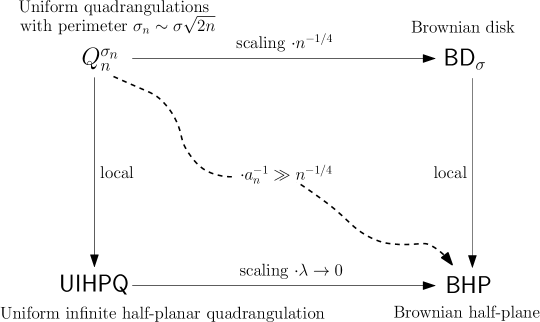
Figure 4: Illustration of [9, Theorem 1] for the regime $\sigma_{n}\sim\sigma\sqrt{2n}$, Theorem 3.3, Theorem 3.6, Corollary 3.17 in the case $\sigma(T)\equiv\sigma\in(0,\infty)$, and Proposition 3.11. Compare with [19, Figure 1].

3.3 Limits of the Brownian disk

Our statements from the last two sections imply various limit results for the Brownian disk $\textup{{BD}}_{T,\sigma(T)}$ when zooming-in around its root. We let $\sigma(\cdot):(0,\infty)\rightarrow(0,\infty)$ be a function of the volume of the Brownian disk that specifies its perimeter. All of the following convergences hold in distribution with respect to the local Gromov-Hausdorff topology when the volume $T$ of the disk tends to infinity.

Corollary 3.15.

Assume $\lim_{T\rightarrow\infty}\sigma(T)=0$. Then

$$\textup{{BD}}_{T,\sigma(T)}\longrightarrow\textup{{BP}}.$$

Corollary 3.16.

Assume $\lim_{T\rightarrow\infty}\sigma(T)=\varsigma\in(0,\infty)$. Then

$$\textup{{BD}}_{T,\sigma(T)}\longrightarrow\textup{{IBD}}_{\varsigma}.$$

Corollary 3.17.

Assume $\sigma(T)\rightarrow\infty$ and $\sigma(T)/T\rightarrow\theta\in[0,\infty)$ as $T\rightarrow\infty$. Then

$$\textup{{BD}}_{T,\sigma(T)}\longrightarrow\textup{{BHP}}_{\theta}.$$

Corollary 3.18.

Assume $\sigma(T)/T\rightarrow\infty$ as $T\rightarrow\infty$. Then

$$\textup{{BD}}_{T,\sigma(T)}\longrightarrow\textup{{ICRT}}.$$

Note that Corollary 3.17 includes the case where $\sigma(T)=\sqrt{T}$. Then $\theta=0$, and since by scaling, $T^{1/4}\cdot\textup{{BD}}_{1}=_{d}\textup{{BD}}_{T,\sqrt{T}}$, it follows that BHP is the tangent cone in distribution of any disk $\textup{{BD}}_{A,L}$ for fixed $A,L>0$. See [15, Section 8.2] for an explanation of this terminology in the context of boundedly compact length spaces, and compare with [19, Theorem 1], where it is shown that the Brownian plane is the tangent cone of the Brownian map at its root.

For completeness, but without going into details, let us mention that identically to the proof of Corollary 3.15 (or Corollary 3.18), a combination of [9, Theorem 1] and [7, Theorem 4] (or  [7, Theorem 4]) leads to the convergences

$$\textup{{BD}}_{T,\sigma}\xrightarrow[]{\sigma\to 0}\textup{{BM}}_{T},\quad\quad\textup{{BD}}_{T,\sigma}\xrightarrow[]{T\to 0}\textup{{CRT}}_{3\sigma}$$

in law in the sense of the global Gromov-Hausdorff topology. The factor $3$ in $\textup{{CRT}}_{3\sigma}$ stems from the particular normalization of the Brownian disk.

Remark/Exercise 3.19.

We leave it as an exercise to the reader to find the right combination of our (or Bettinelli’s, cf. [7]) foregoing results to deduce the following additional results on tangent cones (in distribution, with respect to the local Gromov-Hausdorff topology):

$$\textup{{CRT}}_{T}\xrightarrow[]{T\rightarrow\infty}\textup{{ICRT}},\quad\quad\textup{{BHP}}_{\theta}\xrightarrow[]{\theta\to 0}\textup{{BHP}},\quad\quad\textup{{IBD}}_{\sigma}\xrightarrow[]{\sigma\rightarrow\infty}\textup{{BHP}}.$$

Combining results from the regime $\sigma_{n}\ll\sqrt{n}$ in the first and from $\sigma_{n}\gg\sqrt{n}$ in the second case, one may also prove the following scaling results in law:

$$\textup{{BHP}}_{\theta}\xrightarrow[]{\theta\rightarrow\infty}\textup{{ICRT}}\quad,\quad\quad\textup{{IBD}}_{\sigma}\xrightarrow[]{\sigma\rightarrow 0}\textup{{BP}}.$$

4 Encoding of quadrangulations with a boundary

We will use a variant of the Cori-Vauquelin-Schaeffer [18, 40] bijection developed by Bouttier, Di Francesco and Guitter [12] to encode quadrangulations with a boundary. More specifically, we will encode planar quadrangulation of size $n$ with a boundary of size $2\sigma$ in terms of $\sigma$ trees with $n$ edges in total, which are attached to a discrete bridge of length $\sigma$. We first introduce the encoding objects. Our notation is inspired by [6, 7].

4.1 Encoding in the finite case

4.1.1 Well-labeled tree, forest and bridge

A well-labeled tree $(\tau,(\ell(u))_{u\in\tau})$ of size $|\tau|=n$ consists of a rooted plane tree $\tau$ with $n$ edges together with integer labels $(\ell(u))_{u\in V(\tau)}$ attached to the vertices of $\tau$, such that the root has label $0$, and $|\ell(u)-\ell(v)|\leq 1$ whenever $u$ and $v$ are neighbors.

A well-labeled forest with $\sigma$ trees and $n$ tree edges is a collection $\textup{$\mathfrak{f}$}=(\tau_{0},\ldots,\tau_{\sigma-1})$ of $\sigma$ trees with $n$ edges in total, together with a labeling of vertices $\textup{$\mathfrak{l}$}:\cup_{i=0}^{\sigma-1}V(\tau_{i})\rightarrow\mathbb{Z}$, which has the property that for each $i=0,\ldots,\sigma-1$, the tree $\tau_{i}$ together with the restriction $\textup{$\mathfrak{l}$}\restriction V(\tau_{i})$ forms a well-labeled tree.

The vertex set of $\mathfrak{f}$ is $V(\textup{$\mathfrak{f}$})=\cup_{i=0}^{\sigma-1}V(\tau_{i})$. Note that $|V(\textup{$\mathfrak{f}$})|=n+\sigma$. The size of $\mathfrak{f}$ is given by $|\textup{$\mathfrak{f}$}|=n$, i.e., its number of edges. We write $(0),\ldots,(\sigma-1)$ for the root vertices of $\tau_{0},\ldots,\tau_{\sigma-1}$. If $u$ is a vertex of a tree of $\mathfrak{f}$, $\textup{$\mathfrak{r}$}(u)$ denotes the root of this tree. In particular, the vertex set of the $j$th tree of $\mathfrak{f}$ is the set $\{u\in V(\textup{$\mathfrak{f}$}):\textup{$\mathfrak{r}$}(u)=(j-1)\}$, $j=1,\ldots,\sigma$. We write $t(\textup{$\mathfrak{f}$})=\sigma$ for the number of trees of $\mathfrak{f}$. We will often identify the root vertices with the integers $0,\ldots,\sigma-1$ and consequently regard $\textup{$\mathfrak{r}$}(u)$ as a number.

We call the pair $(\textup{$\mathfrak{f}$},\textup{$\mathfrak{l}$})$ a well-labeled forest and denote by

$$\textup{$\mathfrak{F}$}_{\sigma}^{n}=\{(\textup{$\mathfrak{f}$},\textup{$\mathfrak{l}$}):t(\textup{$\mathfrak{f}$})=\sigma,|\textup{$\mathfrak{f}$}|=n\}$$

the set of all well-labeled forests of size $n$ with $\sigma$ trees.

A bridge of length $\sigma\geq 1$ is a sequence of numbers $(\textup{{b}}(0),\textup{{b}}(1),\ldots,\textup{{b}}(\sigma))$ with $\textup{{b}}(0)=0$ and such that $\textup{{b}}(i+1)-\textup{{b}}(i)\in\mathbb{N}_{0}\cup\{-1\}$, and $\textup{{b}}(\sigma)\leq 0$.

By linear interpolation between integer values, we will view $\textup{{b}}:[0,\sigma]\to\mathbb{R}$ as a continuous function and write $\textup{$\mathfrak{B}$}_{\sigma}\subset\mathcal{C}([0,\sigma],\mathbb{R})$ for the set of all possible bridges of length $\sigma$.

The terminal value $\textup{{b}}(\sigma)$ of a bridge has a special interpretation: It keeps the information where to find the root in the quadrangulation associated to a triplet $((\textup{$\mathfrak{f}$},\textup{$\mathfrak{l}$}),\textup{{b}})\in\textup{$\mathfrak{F}$}_{\sigma}^{n}\times\textup{$\mathfrak{B}$}_{\sigma}$, see Section 4.3 below.

4.1.2 Contour pair and label function

Consider a well-labeled forest $(\textup{$\mathfrak{f}$},\textup{$\mathfrak{l}$})$ of size $n$ with $\sigma$ trees. In order to define its contour pair and label function, it is convenient to associate to $\mathfrak{f}$ a representation in the plane, as depicted in Figure 6: We add $\sigma-1$ edges which link the root vertices $(0),\ldots,(\sigma-1)$, such that vertex $(i-1)$ gets connected to $(i)$ for $i=1,\ldots,\sigma-1$, plus an extra vertex $(\sigma)$ and an extra edge linking $(\sigma-1)$ to $(\sigma)$. We extend $\mathfrak{l}$ to $(\sigma)$ by setting $\textup{$\mathfrak{l}$}((\sigma))=0$. We refer to the segment connecting the roots of $\mathfrak{f}$ and the extra vertex $(\sigma)$ as the floor of $\mathfrak{f}$.

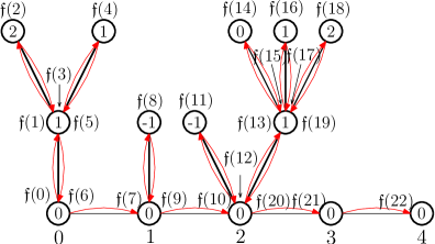
Figure 6: On the left: A proper representation of a finite forest $\mathfrak{f}$ of size $13$ with $4$ trees, together with its facial sequence. The rightmost vertex labeled $4$ is the added extra vertex. On the right: Its contour pair.

The facial sequence $\textup{$\mathfrak{f}$}(0),\ldots,\textup{$\mathfrak{f}$}(2n+\sigma)$ of $\mathfrak{f}$ is the sequence of vertices obtained from exploring (the embedding of) $\mathfrak{f}$ in the contour order, starting from vertex $(0)$. In other words, $\textup{$\mathfrak{f}$}(0),\ldots,\textup{$\mathfrak{f}$}(2n+\sigma-1)$ is given by the sequence of vertices of the discrete contour paths of the trees $\tau_{0},\ldots,\tau_{\sigma-1}$, and the sequence terminates with value $\textup{$\mathfrak{f}$}(2n+\sigma)=(\sigma)$. See, e.g., [30, Section 2] for more on contour paths.

Given a well-labeled forest $(\textup{$\mathfrak{f}$},\textup{$\mathfrak{l}$})$, we define its contour pair $(C_{\textup{$\mathfrak{f}$}},L_{\textup{$\mathfrak{f}$}})$ by

$$C_{\textup{$\mathfrak{f}$}}(j)=d_{\textup{$\mathfrak{f}$}}(\textup{$\mathfrak{f}$}(j),(\sigma))-\sigma,\quad L_{\textup{$\mathfrak{f}$}}(j)=\textup{$\mathfrak{l}$}(\textup{$\mathfrak{f}$}(j)),\quad j=0,\ldots,2n+\sigma.$$

Here, $d_{\textup{$\mathfrak{f}$}}$ denotes the graph distance on the representation of $\mathfrak{f}$ in the plane.

We call $C_{\textup{$\mathfrak{f}$}}$ the contour function of $\mathfrak{f}$, since it is obtained from concatenating the contour paths of the trees $\tau_{0},\ldots,\tau_{\sigma-1}$, with an additional $-1$ step after a tree has been visited. Note that $L_{\textup{$\mathfrak{f}$}}(\textup{$\mathfrak{f}$}(j))=0$ if $\textup{$\mathfrak{f}$}(j)$ lies on the floor of $\mathfrak{f}$. See again Figure 6 for an illustration.

Now consider additionally a bridge $\textup{{b}}\in\textup{$\mathfrak{B}$}_{\sigma}$. Put $\underline{C}_{\textup{$\mathfrak{f}$}}(j)=\min_{[0,j]}C_{\textup{$\mathfrak{f}$}}$. The function

$$\textup{$\mathfrak{L}$}_{\textup{$\mathfrak{f}$}}(j)=L_{\textup{$\mathfrak{f}$}}(j)+\textup{{b}}(-\underline{C}_{\textup{$\mathfrak{f}$}}(j)),\quad j=0,\dots,2n+\sigma,$$

is called the label function associated to $((\textup{$\mathfrak{f}$},\textup{$\mathfrak{l}$}),\textup{{b}})$. The label function plays an important role in measuring distances in the quadrangulation associated through the Bouttier-Di Francesco-Guitter bijection, see Section 4.5.1.

By linear interpolation between integers, we extend all three functions $C_{\textup{$\mathfrak{f}$}}$, $L_{\textup{$\mathfrak{f}$}}$ and $\textup{$\mathfrak{L}$}_{\textup{$\mathfrak{f}$}}$ to continuous real-valued functions on $[0,2n+\sigma]$.

4.2 Encoding in the infinite case

We next introduce the infinite analogs of the objects from the previous section. They will encode certain infinite quadrangulations with an infinite boundary.

4.2.1 Well-labeled infinite forest and infinite bridge

A well-labeled infinite forest is an infinite collection $\textup{$\mathfrak{f}$}=(\tau_{i},i\in\mathbb{Z})$ of finite rooted plane trees, together with a labeling of vertices $\textup{$\mathfrak{l}$}:\cup_{i\in\mathbb{Z}}V(\tau_{i})\rightarrow\mathbb{Z}$ such that for each $i\in\mathbb{Z}$, $\tau_{i}$ together with the restriction of $\mathfrak{l}$ to $V(\tau_{i})$ forms a well-labeled tree.

We write again $(k)$ for the root vertex of $\tau_{k}$ and often identify $(k)$ with $k\in\mathbb{Z}$. We call the pair $(\textup{$\mathfrak{f}$},\textup{$\mathfrak{l}$})$ an well-labeled infinite forest and denote by $\textup{$\mathfrak{F}$}_{\infty}$ the set of all well-labeled infinite forests.

An infinite bridge is a sequence of numbers $\textup{{b}}=(\textup{{b}}(i),i\in\mathbb{Z}\cup\{\partial\})$ with $\textup{{b}}(0)=0$, $\textup{{b}}(i+1)-\textup{{b}}(i)\in\mathbb{N}_{0}\cup\{-1\}$ for all $i\in\mathbb{Z}$ and $\textup{{b}}(\partial)\in\{\textup{{b}}(-1)-1,\ldots,0\}$.

The extra value $\textup{{b}}(\partial)$ will keep track of the position of the root in the quadrangulation. Often, we consider only the values $\textup{{b}}(i)$, $i\in\mathbb{Z}$, and then view b as a continuous function from $\mathbb{R}$ to $\mathbb{R}$, by linear interpolation between integer values. We write $\textup{$\mathfrak{B}$}_{\infty}$ for the set of all infinite bridges b which have the property that $\inf_{i\in\mathbb{N}}\textup{{b}}(i)=-\infty$, and $\inf_{i\in\mathbb{N}}\textup{{b}}(-i)=-\infty$.

4.2.2 Contour pair and label function in the infinite case

We consider a well-labeled infinite forest $(\textup{$\mathfrak{f}$},\textup{$\mathfrak{l}$})\in\textup{$\mathfrak{F}$}_{\infty}$. Again, we view $\mathfrak{f}$ as a graph properly embedded in the plane (Figure 7): We identify the set of roots of the trees of $\mathfrak{f}$ with $\mathbb{Z}$ and connect neighboring roots by an edge. We obtain what we call the floor of $\mathfrak{f}$. The trees $\tau_{i}$ of $\mathfrak{f}$ are drawn in the upper half-plane and attached to the floor.

The facial sequence $(\textup{$\mathfrak{f}$}(i),i\in\mathbb{Z})$ of $\mathfrak{f}$ is defined as follows: $(\textup{$\mathfrak{f}$}(0),\textup{$\mathfrak{f}$}(1),\ldots)$ is the sequence of vertices of the contour paths of the trees $\tau_{i},i\in\mathbb{N}_{0}$, in the contour order, starting from the root of the tree $\tau_{0}$, and $(\textup{$\mathfrak{f}$}(-1),\textup{$\mathfrak{f}$}(-2),\ldots)$ is given by the sequence of vertices of the contour paths $\tau_{-1},\tau_{-2},\ldots$, in the counterclockwise order, starting from the root of the tree $\tau_{-1}$.

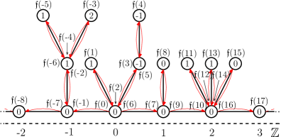
Figure 7: On the left: A proper representation of an infinite forest $\mathfrak{f}$, together with its facial sequence. On the right: Its contour function.

In analogy to the finite case, given a well-labeled infinite tree $(\textup{$\mathfrak{f}$},\textup{$\mathfrak{l}$})$, its contour pair $(C_{\textup{$\mathfrak{f}$}},L_{\textup{$\mathfrak{f}$}})$ is a tuple functions defined via

$$C_{\textup{$\mathfrak{f}$}}(j)=d_{\textup{$\mathfrak{f}$}}(\textup{$\mathfrak{f}$}(j),\textup{$\mathfrak{r}$}(\textup{$\mathfrak{f}$}(j)))-\textup{$\mathfrak{r}$}(\textup{$\mathfrak{f}$}(j)),\quad L_{\textup{$\mathfrak{f}$}}(j)=\textup{$\mathfrak{l}$}(\textup{$\mathfrak{f}$}(j)),\quad j\in\mathbb{Z},$$

where $d_{\textup{$\mathfrak{f}$}}$ is the graph distance on the embedding of $\mathfrak{f}$, and $\textup{$\mathfrak{r}$}(\textup{$\mathfrak{f}$}(j))$ denotes the root of the tree $\textup{$\mathfrak{f}$}(j)$ belongs to. Be aware of the small abuse of notation: In the expression for $C_{\textup{$\mathfrak{f}$}}$, $\textup{$\mathfrak{r}$}(\textup{$\mathfrak{f}$}(j))$ is first viewed as a vertex and then as an integer.

Note that $\lim_{j\rightarrow\infty}C_{\textup{$\mathfrak{f}$}}(j)\rightarrow-\infty$ and $\lim_{j\rightarrow-\infty}C_{\textup{$\mathfrak{f}$}}(j)\rightarrow+\infty$ for every infinite forest. As for a finite forest, we call $C_{\textup{$\mathfrak{f}$}}$ the contour function of $\mathfrak{f}$.

If additionally $\textup{{b}}\in\textup{$\mathfrak{B}$}_{\infty}$, we define the label function associated to $((\textup{$\mathfrak{f}$},\textup{$\mathfrak{l}$}),\textup{{b}})$ by

$$\textup{$\mathfrak{L}$}_{\textup{$\mathfrak{f}$}}(j)=L_{\textup{$\mathfrak{f}$}}(j)+\textup{{b}}(\underline{C}_{\textup{$\mathfrak{f}$}}(j)),\quad j\in\mathbb{Z},\quad\textup{$\mathfrak{L}$}_{\textup{$\mathfrak{f}$}}(\partial)=\textup{{b}}(\partial),$$

where $\underline{C}_{\textup{$\mathfrak{f}$}}(j)=\inf_{(-\infty,j]}C_{\textup{$\mathfrak{f}$}}$ for $j<0$ and $\underline{C}_{\textup{$\mathfrak{f}$}}(j)=\min_{[0,j]}C_{\textup{$\mathfrak{f}$}}$ for $j\geq 0$, as above.

Again by linear interpolation between integers, we view $C_{\textup{$\mathfrak{f}$}},L_{\textup{$\mathfrak{f}$}}$ and $\textup{$\mathfrak{L}$}_{\textup{$\mathfrak{f}$}}$ as continuous functions on $\mathbb{R}$.

4.3 Bouttier-Di Francesco-Guitter bijection

Recall that a rooted quadrangulation with a boundary comes with a distinguished edge along the boundary, the root edge, whose origin is the root vertex. We write $\mathcal{Q}_{n}^{\sigma}$ for the set of all rooted quadrangulations with $n$ inner faces and a boundary of size $2\sigma$.

A pointed quadrangulation with a boundary is a pair $(\textup{$\mathfrak{q}$},v^{\bullet})$, where $\mathfrak{q}$ is a rooted quadrangulation with a boundary and $v^{\bullet}\in V(\textup{$\mathfrak{q}$})$ is a distinguished vertex. The set of all rooted pointed quadrangulations with $n$ internal faces and $2\sigma$ boundary edges is denoted by

$$\mathcal{Q}_{n,\sigma}^{\bullet}=\left\{(\textup{$\mathfrak{q}$},v^{\bullet}):\textup{$\mathfrak{q}$}\in\mathcal{Q}_{n}^{\sigma},v^{\bullet}\in V(\textup{$\mathfrak{q}$})\right\}.$$

4.3.1 The finite case

The Bouttier-Di Francesco-Guitter bijection [12] provides us with a bijection

$$\Phi_{n}:\textup{$\mathfrak{F}$}_{\sigma}^{n}\times\textup{$\mathfrak{B}$}_{\sigma}\longrightarrow\mathcal{Q}_{n,\sigma}^{\bullet}.$$

We shall here content ourselves with the description of the mapping from the encoding objects to the quadrangulations. We follow largely the presentation in [7], where also a description of the reverse direction can be found.

In this regard, let $((\textup{$\mathfrak{f}$},\textup{{b}}),\textup{$\mathfrak{l}$})\in\textup{$\mathfrak{F}$}_{\sigma}^{n}\times\textup{$\mathfrak{B}$}_{\sigma}$. Out of this triplet, we will now construct a rooted pointed quadrangulation $(\textup{$\mathfrak{q}$},v^{\bullet})\in\mathcal{Q}_{n,\sigma}^{\bullet}$. Recall the facial sequence $\textup{$\mathfrak{f}$}(0),\ldots,\textup{$\mathfrak{f}$}(2n+\sigma)$ of $\mathfrak{f}$ obtained from exploring the trees of $\mathfrak{f}$ in the contour order, as well as the associated label function $\textup{$\mathfrak{L}$}_{\textup{$\mathfrak{f}$}}$. We view $\mathfrak{f}$ as embedded in the plane (as explained above) and add an additional vertex $v^{\bullet}$ inside the only face of $\mathfrak{f}$, with label $\textup{$\mathfrak{L}$}_{\textup{$\mathfrak{f}$}}(v^{\bullet})=-\infty$.

The vertex set of $\mathfrak{q}$ is given by $V(\textup{$\mathfrak{f}$})\cup\{v^{\bullet}\}$. Note that by definition, the additional vertex $(\sigma)$ which forms part of the embedding of $\mathfrak{f}$ is not an element of $V(\textup{$\mathfrak{f}$})$. In order to specify the edges between the vertices of $\mathfrak{q}$, we define for $i=0,\ldots,2n+\sigma-1$ the successor $\textup{succ}(i)\in\{0,\ldots,2n+\sigma-1\}\cup\{\infty\}$ of $i$ to be the first number $k$ in the list $(i+1,\ldots,2n+\sigma-1,0,\ldots,i-1)$ with the property that $\textup{$\mathfrak{L}$}_{\textup{$\mathfrak{f}$}}(k)=\textup{$\mathfrak{L}$}_{\textup{$\mathfrak{f}$}}(i)-1$, with $\textup{succ}(i)=\infty$ if there is no such number. Letting $\textup{$\mathfrak{f}$}(\infty)=v^{\bullet}$, we now follow the facial sequence of $\mathfrak{f}$ and draw for every $i=0,\ldots,2n+\sigma-1$ an arc between $\textup{$\mathfrak{f}$}(i)$ and $\textup{$\mathfrak{f}$}(\textup{succ}(i))$, in such a way that it neither crosses arcs that were previously drawn, nor edges of the embedding of $\mathfrak{f}$. Since any vertex of $\mathfrak{f}$ which is not a leaf is visited at least twice in the contour exploration, there can be several arcs connecting $\textup{$\mathfrak{f}$}(i)$ and $\textup{$\mathfrak{f}$}(\textup{succ}(i))$. By a small abuse of language, we therefore speak of the arc connecting $i$ to $\textup{succ}(i)$ and write

$$i\curvearrowright\textup{succ}(i)\quad\hbox{or}\quad i\curvearrowleft\textup{succ}(i)$$

for the oriented arc from $i$ towards $\textup{succ}(i)$ or from $\textup{succ}(i)$ towards $i$, respectively.

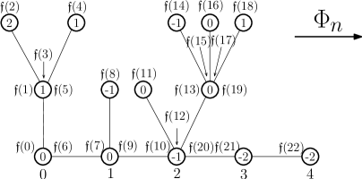
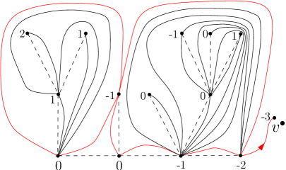
Figure 8: The Bouttier-Di Francesco-Guitter bijection $\Phi_{n}$ applied to an element $((\textup{$\mathfrak{f}$},\textup{$\mathfrak{l}$}),\textup{{b}})\in\textup{$\mathfrak{F}$}_{\sigma}^{n}\times\textup{$\mathfrak{B}$}_{\sigma}$. The forest $\mathfrak{f}$ is the same as in Figure 6, but the labels are shifted by the values of the bridge b. The (non-simple) boundary of the associated quadrangulation on the left is represented in red. Note that the extra vertex $v^{\bullet}$ is in this example a boundary vertex. The rightmost vertex $\textup{$\mathfrak{f}$}(22)=(4)$ on the left is not a vertex of the quadrangulation. Its label $-2$ captures the information where to find the root edge, which is indicated by an arrow.

The arcs between the vertices $V(\textup{$\mathfrak{f}$})\cup\{v^{\bullet}\}$ form the edges of $\mathfrak{q}$, and it remains to specify the root edge of $\mathfrak{q}$: The root vertex is given by $\textup{$\mathfrak{f}$}(\textup{succ}^{-\textup{{b}}(\sigma)}(0))$, and the root edge is in case $\textup{{b}}(\sigma)>\textup{{b}}(\sigma-1)-1$ given by $\textup{succ}^{-\textup{{b}}(\sigma)}(0)\curvearrowright\textup{succ}^{-\textup{{b}}(\sigma)+1}(0)$, and in case $\textup{{b}}(\sigma)=\textup{{b}}(\sigma-1)-1$ by $2n+\sigma-1\curvearrowleft\textup{succ}(2n+\sigma-1)$. Note that in the second case, we have indeed $\textup{$\mathfrak{f}$}(\textup{succ}(2n+\sigma-1))=\textup{$\mathfrak{f}$}(\textup{succ}^{-\textup{{b}}(\sigma)}(0))$, i.e., $\textup{succ}(2n+\sigma-1)$ is the root vertex.

4.3.2 The infinite case

Let $\mathcal{Q}$ denote the completion of the space of all rooted finite quadrangulations with a boundary with respect to $d_{\textup{map}}$. We extend $\Phi_{n}$ to a mapping

$$\Phi:\left({\cup}_{n,\sigma\in\mathbb{N}}\textup{$\mathfrak{F}$}_{\sigma}^{n}\times\textup{$\mathfrak{B}$}_{\sigma}\right)\cup\left(\textup{$\mathfrak{F}$}_{\infty}\times\textup{$\mathfrak{B}$}_{\infty}\right)\longrightarrow\mathcal{Q}$$

as follows. For elements $((\textup{$\mathfrak{f}$},\textup{$\mathfrak{l}$}),\textup{{b}})\in\textup{$\mathfrak{F}$}_{\sigma}^{n}\times\textup{$\mathfrak{B}$}_{\sigma}$, we let $\Phi(((\textup{$\mathfrak{f}$},\textup{$\mathfrak{l}$}),\textup{{b}}))=\Phi_{n}((\textup{$\mathfrak{f}$},\textup{$\mathfrak{l}$}),\textup{{b}})$, where we view the latter as an element in $\mathcal{Q}_{n}^{\sigma_{n}}$, by simply forgetting its distinguished vertex.

Now let $((\textup{$\mathfrak{f}$},\textup{$\mathfrak{l}$}),\textup{{b}})\in\textup{$\mathfrak{F}$}_{\infty}\times\textup{$\mathfrak{B}$}_{\infty}$. For $i\in\mathbb{Z}$, we define the successor $\textup{succ}_{\infty}(i)$ to be the smallest number $k$ greater than $i$ such that $\textup{$\mathfrak{L}$}_{\textup{$\mathfrak{f}$}}(k)=\textup{$\mathfrak{L}$}_{\textup{$\mathfrak{f}$}}(i)-1$. Note that since $\inf_{i\in\mathbb{N}}\textup{{b}}(i)=-\infty$, the definition make sense. We consider a proper embedding of $\mathfrak{f}$ in the plane as described above and draw an arc between $\textup{$\mathfrak{f}$}(i)$ and $\textup{$\mathfrak{f}$}(\textup{succ}_{\infty}(i))$, for any $i\in\mathbb{Z}$, as indicated by Figure 9. Again we can do this in a way such that arcs do not cross. The vertex set of $\Phi(((\textup{$\mathfrak{f}$},\textup{$\mathfrak{l}$}),\textup{{b}}))$ is given by $V(\textup{$\mathfrak{f}$})$, and the edges are the arcs we constructed. Finally, we follow a rooting convention which is analogous to the finite case (we adapt the notion $i\curvearrowright\textup{succ}_{\infty}(i)$ in the obvious way): The root vertex is given by $\textup{$\mathfrak{f}$}(\textup{succ}_{\infty}^{-\textup{{b}}(\partial)}(0))$, and the root edge is in case $\textup{{b}}(\partial)>\textup{{b}}(-1)-1$ given by $\textup{succ}_{\infty}^{-\textup{{b}}(\partial)}(0)\curvearrowright\textup{succ}^{-\textup{{b}}(\partial)+1}(0)$, and in case $\textup{{b}}(\partial)=\textup{{b}}(-1)-1$ by $-1\curvearrowleft\textup{succ}_{\infty}(-1)$.

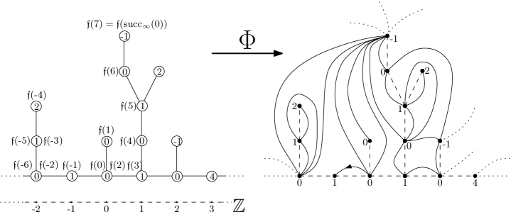
Figure 9: The Bouttier-Di Francesco-Guitter mapping applied to an element $((\textup{$\mathfrak{f}$},\textup{$\mathfrak{l}$}),\textup{{b}})\in\textup{$\mathfrak{F}$}_{\infty}\times\textup{$\mathfrak{B}$}_{\infty}$. The successor of $0$ is $7$, which is also the successor of $-6,-2,1,2,4,6$. The vertex labels are given by $\textup{$\mathfrak{L}$}_{\textup{$\mathfrak{f}$}}$, as in Figure 8. The root edge of the map is the oriented arc $-1\curvearrowleft\textup{succ}_{\infty}(-1)$ indicated by an arrow.

Remark 4.1.

Notice that a triplet $((\textup{$\mathfrak{f}$},\textup{{b}}),\textup{$\mathfrak{l}$})$ in $\textup{$\mathfrak{F}$}_{\sigma}^{n}\times\textup{$\mathfrak{B}$}_{\sigma}$ or in $\textup{$\mathfrak{F}$}_{\infty}\times\textup{$\mathfrak{B}$}_{\infty}$ is uniquely determined by its associated contour and label functions $(C_{\textup{$\mathfrak{f}$}},\textup{$\mathfrak{L}$}_{\textup{$\mathfrak{f}$}})$. In particular, it makes sense to speak of the quadrangulation associated to $(C_{\textup{$\mathfrak{f}$}},\textup{$\mathfrak{L}$}_{\textup{$\mathfrak{f}$}})$. The distinguished vertex $v^{\bullet}$ in the finite case will play no particular role in our statements, since we view quadrangulations as metric spaces pointed at their root vertices.

4.4 Construction of the UIHPQ

We first introduce a $\textup{$\mathfrak{F}$}_{\infty}$-valued random element $(\textup{$\mathfrak{f}$}_{\infty},\textup{$\mathfrak{l}$}_{\infty})$ together with a $\textup{$\mathfrak{B}$}_{\infty}$-valued random element $\textup{{b}}_{\infty}$, which will encode the UIHPQ.

4.4.1 Uniformly labeled critical infinite forest

Let $\tau$ be a finite random plane tree. Conditionally on $\tau$, we assign a sequence of i.i.d random variables with the uniform distribution on $\{-1,0,1\}$ to the edges of $\tau$. The label $\ell(u)$ of a vertex $u$ of $\tau$ is defined to be the sum of the random variables along the edges of the (unique) path from the root to $u$. Such a random labeling $\ell:V(\tau)\rightarrow\mathbb{Z}$ is referred to as a uniform labeling. If the tree $\tau$ is a Galton-Watson tree with a geometric offspring distribution of parameter $1/2$, we say that $\tau$ is a critical geometric Galton-Watson tree. If $\ell$ is a uniform labeling of $\tau$, we refer to the pair $(\tau,(\ell(u))_{u\in\tau})$ as a uniformly labeled critical geometric Galton-Watson tree.

A uniformly labeled critical infinite forest is a random element $(\textup{$\mathfrak{f}$}_{\infty},\textup{$\mathfrak{l}$}_{\infty})$ taking values in $\textup{$\mathfrak{F}$}_{\infty}$ such that the pairs $(\tau_{i},\textup{$\mathfrak{l}$}_{\infty}\restriction V(\tau_{i}))$, $i\in\mathbb{Z}$, are independent uniformly labeled critical geometric Galton-Watson trees.

4.4.2 Uniform infinite bridge

Let $\textup{{b}}_{\infty}=(\textup{{b}}_{\infty}(i),i\in\mathbb{Z})$ be a two-sided random walk starting from $0$ at time $0$, i.e., $\textup{{b}}_{\infty}(0)=0$, which has independent increments given by

$$\mathbb{P}(\textup{{b}}_{\infty}(i)-\textup{{b}}_{\infty}(i-1)=k)=2^{-k-2},\quad k\in\mathbb{N}_{0}\cup\{-1\},\quad\hbox{for }i\in\mathbb{Z}\setminus\{0\},$$

and

$$\mathbb{P}(-\textup{{b}}_{\infty}(-1)=k)=(k+2)2^{-(k+3)},\quad k\in\mathbb{N}_{0}\cup\{-1\}.$$

Note that $-\textup{{b}}_{\infty}(-1)$ has same law as $G+G^{\prime}-1$ for $G$ and $G^{\prime}$ two independent geometric random variables of parameter $1/2$. This follows from the well-known fact that $G+G^{\prime}+1$ is distributed as a size-biased geometric random variable. We refer to Section 4.5.2 for more explanations. Next, given $\textup{{b}}_{\infty}(-1)$, we let $\textup{{b}}_{\infty}(\partial)$ be a uniformly distributed random variable in $\{\textup{{b}}_{\infty}(-1)-1,\ldots,0\}$, independent of everything else.

We call the random element $\textup{{b}}_{\infty}=(\textup{{b}}_{\infty}(i),i\in\mathbb{Z}\cup\{\partial\})$ with values in $\textup{$\mathfrak{B}$}_{\infty}$ the uniform infinite bridge.

We review now the construction of the UIHPQ given in [22]. Note that there, the encoding is defined in a slightly different (but equivalent) manner, and the root edge is oriented in the opposite direction. The following definition is justified by Proposition 3.11.

Definition 4.2.

Let $(\textup{$\mathfrak{f}$}_{\infty},\textup{$\mathfrak{l}$}_{\infty})$ be a uniformly labeled critical infinite forest, and let $\textup{{b}}_{\infty}$ be a uniform infinite bridge independent of $(\textup{$\mathfrak{f}$}_{\infty},\textup{$\mathfrak{l}$}_{\infty})$. The uniform infinite half-planar quadrangulation UIHPQ is the (rooted) random infinite quadrangulation $Q_{\infty}^{\infty}=(V(Q_{\infty}^{\infty}),d_{\textup{gr}},\rho)$ with an infinite boundary obtained from applying the Bouttier-Di Francesco-Guitter mapping $\Phi$ to $((\textup{$\mathfrak{f}$}_{\infty},\textup{$\mathfrak{l}$}_{\infty}),\textup{{b}}_{\infty})$.

In [22], it was shown that in the sense of $d_{\textup{map}}$, there are the weak convergences

$$Q_{n}^{\sigma_{n}}\xrightarrow[]{n\to\infty}Q_{\infty}^{\sigma},\quad Q_{\infty}^{\sigma}\xrightarrow[]{\sigma\to\infty}Q_{\infty}^{\infty},$$

where $Q_{\infty}^{\sigma}$ is the so-called (rooted) uniform infinite planar quadrangulation with a boundary of perimeter $2\sigma$. We also point at the recent work [16], where a construction of the UIHPQ with a positivity constraint on labels is given, similarly to the Chassaing-Durhuus construction [17] of the UIPQ.

Remark 4.3.

We stress that while we use the notation $(\textup{$\mathfrak{f}$},\textup{$\mathfrak{l}$})$ for both a finite or infinite (deterministic) well-labeled forest, and similarly, b represents a finite or infinite bridge, $(\textup{$\mathfrak{f}$}_{\infty},\textup{$\mathfrak{l}$}_{\infty})\in\textup{$\mathfrak{F}$}_{\infty}$ and $\textup{{b}}_{\infty}\in\textup{$\mathfrak{B}$}_{\infty}$ will always stand for random elements with the particular law just described. We will implicitly assume that $\textup{{b}}_{\infty}$ is independent of $(\textup{$\mathfrak{f}$}_{\infty},\textup{$\mathfrak{l}$}_{\infty})$. Similarly, for given $\sigma_{n}$, $((\textup{$\mathfrak{f}$}_{n},\textup{$\mathfrak{l}$}_{n}),\textup{{b}}_{n})$ will denote a random element with the uniform distribution on $\textup{$\mathfrak{F}$}_{n}^{\sigma_{n}}\times\textup{$\mathfrak{B}$}_{\sigma_{n}}$, see Section 4.5.4.

4.5 Some ramifications

We gather here some consequences and remarks which we will tacitly use in the following. We begin with some observations concerning the Bouttier-Di Francesco-Guitter bijection.

4.5.1 Distances

Let $(\textup{$\mathfrak{q}$},v^{\bullet})\in\mathcal{Q}_{n,\sigma}^{\bullet}$ be a (rooted) pointed quadrangulations of size $n$ with a boundary of size $2\sigma$. Then $(\textup{$\mathfrak{q}$},v^{\bullet})$ corresponds to a pair $((\textup{$\mathfrak{f}$},\textup{$\mathfrak{l}$}),\textup{{b}})\in\textup{$\mathfrak{F}$}_{\sigma}^{n}\times\textup{$\mathfrak{B}$}_{\sigma}$ via the Bouttier-Di Francesco-Guitter bijection, and the sets $V(\textup{$\mathfrak{q}$})\setminus\{v^{\bullet}\}$ and $V(\textup{$\mathfrak{f}$})$ are identified through this bijection. Recall that the label function $\textup{$\mathfrak{L}$}=\textup{$\mathfrak{L}$}_{f}$ represents the labels in the forest shifted tree by tree according to the values of the bridge b. By a slight abuse of notation, we will view $\mathfrak{L}$ also as a function on $V(\textup{$\mathfrak{q}$})\setminus\{v^{\bullet}\}$ (or $V(\textup{$\mathfrak{f}$})$): If $v\in V(\textup{$\mathfrak{q}$})\setminus\{v^{\bullet}\}$, there is at least one $i\in\{0,\ldots,2n+\sigma-1\}$ such that $v$ is visited in the $i$th step of the contour exploration, and we let $\textup{$\mathfrak{L}$}(v)=\textup{$\mathfrak{L}$}(i)$. Note that this definition makes sense, since $\textup{$\mathfrak{L}$}(i)=\textup{$\mathfrak{L}$}(j)$ if $\textup{$\mathfrak{f}$}(i)=\textup{$\mathfrak{f}$}(j)$.

Write $d_{{\bf q}}$ for the graph distance on ${\bf q}$. From the description of the bijection above, we deduce that

$$d_{{\bf q}}(u,v^{\bullet})=\textup{$\mathfrak{L}$}(u)-\min\textup{$\mathfrak{L}$}+1.$$ (4.1)

Moreover, if $v_{0}$ is the root vertex of $\mathfrak{q}$, we know that its distance to vertex $\textup{$\mathfrak{f}$}(0)=(0)$ is

$$d_{{\bf q}}(v_{0},(0))=-\textup{{b}}(\sigma).$$ (4.2)

In general, there is no simple formula for distances in $\mathfrak{q}$. However, as we explain next, there exist lower and upper bounds in terms of $\mathfrak{L}$.

We first discuss a lower bound. If $u,v\in V(\textup{$\mathfrak{f}$})$ are vertices of the same tree $\tau$ of $\mathfrak{f}$, i.e., $\textup{$\mathfrak{r}$}(u)=\textup{$\mathfrak{r}$}(v)$, we let $[[u,v]]$ be the vertex set of the unique injective path in $\tau$ connecting $u$ to $v$. If $(i)$, $(j)$ are two tree roots of $\mathfrak{f}$ with $i<j$, we let $[[(i),(j)]]$ denote the sequence of root vertices $(i),(i+1),\ldots,(j)$. For the remaining cases, if $\textup{$\mathfrak{r}$}(u)<\textup{$\mathfrak{r}$}(v)$, we put

$$[[u,v]]=[[u,\textup{$\mathfrak{r}$}(u)]]\cup[[\textup{$\mathfrak{r}$}(u),\textup{$\mathfrak{r}$}(v)]]\cup[[v,\textup{$\mathfrak{r}$}(v)]],$$

whereas if $\textup{$\mathfrak{r}$}(v)<\textup{$\mathfrak{r}$}(u)$, we let

$$[[u,v]]=[[u,\textup{$\mathfrak{r}$}(u)]]\cup[[\textup{$\mathfrak{r}$}(u),(\sigma-1)]]\cup[[(0),\textup{$\mathfrak{r}$}(v)]]\cup[[v,\textup{$\mathfrak{r}$}(v)]].$$

Now let $u,v\in V(\textup{$\mathfrak{q}$})\setminus\{v^{\bullet}\}$. The so-called cactus bound states that

$$d_{{\bf q}}(u,v)\geq\textup{$\mathfrak{L}$}(u)+\textup{$\mathfrak{L}$}(v)-2\max\left\{\min_{[[u,v]]}\textup{$\mathfrak{L}$},\min_{[[v,u]]}\textup{$\mathfrak{L}$}\right\}.$$ (4.3)

See [34, Proposition 2.3.8] for a proof in a slightly different context, which is readily adapted to our setting. Since vertex $(0)$ has label $\textup{$\mathfrak{L}$}(0)=0$ and $\mathfrak{L}$ coincides with the values of the bridge along the floor of $\mathfrak{f}$, the distance $d_{{\bf q}}((0),u)$ for $u\in V(\textup{$\mathfrak{q}$})\setminus\{v^{\bullet}\}$ is lower bounded by

$$d_{{\bf q}}((0),u)\geq-\max\left\{\min_{[0,\textup{$\mathfrak{r}$}(u)]}\textup{{b}},\min_{[\textup{$\mathfrak{r}$}(u),\sigma-1]}\textup{{b}}\right\}.$$ (4.4)

For an upper bound of $d_{{\bf q}}(u,v)$ when $u,v\in V(\textup{$\mathfrak{q}$})\setminus\{v^{\bullet}\}$, choose $i,j\in\{0,\ldots,2n+\sigma-1\}$ such that $\textup{$\mathfrak{f}$}(i)=u$ and $\textup{$\mathfrak{f}$}(j)=v$. Define

$$\overrightarrow{[i,j]}=\left\{\begin{array}[]{l@{\quad\mbox{if }}l}\{i,\ldots,j\}&i\leq j\\ \{i,\ldots,2n+\sigma-1\}\cup\{0,\ldots,j\}&i>j\end{array}\right..$$

Then there is the upper bound (see [32, Lemma 3] for a proof)

$$d_{{\bf q}}(u,v)\leq\textup{$\mathfrak{L}$}(u)+\textup{$\mathfrak{L}$}(v)-2\max\left\{\min_{\overrightarrow{[i,j]}}\textup{$\mathfrak{L}$}(\textup{$\mathfrak{f}$}),\,\min_{\overrightarrow{[j,i]}}\textup{$\mathfrak{L}$}(\textup{$\mathfrak{f}$})\right\}+2.$$ (4.5)

Bounds similar to (4.3), (4.4) and (4.5) can be formulated for infinite quadrangulations $\textup{$\mathfrak{q}$}_{\infty}$ constructed from triplets $((\textup{$\mathfrak{f}$},\textup{{b}}),\textup{$\mathfrak{l}$})\in\textup{$\mathfrak{F}$}_{\infty}\times\textup{$\mathfrak{B}$}_{\infty}$. For example, if $u,v\in V(\textup{$\mathfrak{f}$})$ with $\textup{$\mathfrak{r}$}(u)\leq\textup{$\mathfrak{r}$}(v)$, the cactus bound (4.3) reads

$$d_{{\bf q}_{\infty}}(u,v)\geq\textup{$\mathfrak{L}$}(u)+\textup{$\mathfrak{L}$}(v)-2\min_{[[u,v]]}\textup{$\mathfrak{L}$}.$$ (4.6)

4.5.2 Bridges

We will need some properties of elements in $\textup{$\mathfrak{B}$}_{\sigma}$. Firstly, as it is shown in [7, Lemma 6], by identifying a bridge $(\textup{{b}}(i),0\leq i\leq\sigma)\in\textup{$\mathfrak{B}$}_{\sigma}$ with the sequence

$$\big{(}\underbrace{+1,+1,\dots,+1}_{\textup{{b}}(0)-\textup{{b}}(\sigma)\textup{ times}},-1,\underbrace{+1,+1,\dots,+1}_{\textup{{b}}(1)-\textup{{b}}(0)+1\textup{ times}},-1,\underbrace{+1,+1,\dots,+1}_{\textup{{b}}(2)-\textup{{b}}(1)+1\textup{ times}},\dots,-1,\underbrace{+1,+1,\dots,+1}_{\textup{{b}}(\sigma)-\textup{{b}}(\sigma-1)+1\textup{ times}}\big{)},$$ (4.7)

one obtains a one-to-one correspondence between $\textup{$\mathfrak{B}$}_{\sigma}$ and the set of sequences in $\{-1,+1\}^{2\sigma}$ counting exactly $\sigma$ times the number $-1$. As a consequence, $|\textup{$\mathfrak{B}$}_{\sigma}|={2\sigma\choose\sigma}$.

It is helpful to adopt the following point of view. Imagine that we mark $\sigma$ points on the discrete circle $\mathbb{Z}/\textup{mod}\,2\sigma$ uniformly at random. Marked points obtain label $-1$, unmarked points label $+1$. Now choose uniformly at random one of the $2\sigma$ circle points as the origin. By walking around the circle in the clockwise order starting from the chosen origin, one observes a sequence of consecutive $+1$ and $-1$, which is distributed as (4.7) when b is chosen uniformly at random in $\textup{$\mathfrak{B}$}_{\sigma}$. In particular, $(\textup{{b}}(\sigma)-\textup{{b}}(\sigma-1)+1)+(\textup{{b}}(0)-\textup{{b}}(\sigma)+1)=-\textup{{b}}(\sigma-1)+2$ has the law of a size-biased pick among all $\sigma$ consecutive segments of the form $(+1,+1,\ldots,+1,-1)$. When $\sigma$ tends to infinity, it is readily seen that $-\textup{{b}}(\sigma-1)$ converges in distribution to $G+G^{\prime}-1$, where $G$ and $G^{\prime}$ are two independent geometric random variables of parameter $1/2$. This explains the particular law of the increment $-\textup{{b}}_{\infty}(-1)$ of a uniform infinite bridge $\textup{{b}}_{\infty}$ that forms part of the encoding of the UIHPQ.

Next, let $(X_{i},i\in\mathbb{N})$ be a sequence of i.i.d. random variables with distribution

$$\mathbb{P}(X_{1}=k)=2^{-k-2},\quad k\geq-1.$$

Put $\Sigma_{j}=\sum_{i=1}^{j}X_{i}$, with $\Sigma_{0}=0$. Fix $0\leq k\leq\sigma$, and denote by $S^{(k)}=(S^{(k)}(j),j=0,\ldots,\sigma)$ the discrete bridge distributed as $(\Sigma_{j},j=0,\ldots,\sigma)$ conditioned on $\{\Sigma_{\sigma}=-k\}$. Then the above considerations imply that $S^{(k)}$ is uniformly distributed over the set $\{\textup{{b}}\in\textup{$\mathfrak{B}$}_{\sigma}:\textup{{b}}(\sigma)=-k\}$. Secondly, we can compute

$$\mathbb{P}\left(\textup{{b}}(\sigma)=-k\right)=\frac{1}{2}\frac{(2\sigma-k-1)!}{(2\sigma-1)!}\frac{\sigma!}{(\sigma-k)!}\leq 2^{-k},$$ (4.8)

and $\mathbb{P}\left(\textup{{b}}(\sigma)=-k\right)\rightarrow 2^{-k-1}$ as $\sigma\rightarrow\infty$. See [7, Proof of Proposition 7] for a complete argument.

4.5.3 Forests

In the rest of this paper, we will often use the following well-known fact (see, e.g., [30, Section 2]): If $\textup{$\mathfrak{f}$}=(\tau_{0},\ldots,\tau_{\sigma-1})$ is chosen uniformly at random among all forests with $\sigma$ trees and $n$ edges, then the corresponding discrete contour path $(C_{\textup{$\mathfrak{f}$}}(j),j=0,\ldots,\sigma)$, is distributed as a simple random walk path starting at $0$ and conditioned to end at $-\sigma$ at time $2n+\sigma$. As a consequence, we have for $j\in\{0,\ldots,\sigma\}$ and positive integers $k_{i}$,

$$\mathbb{P}\left(|\tau_{0}|=k_{0},\ldots,|\tau_{j-1}|=k_{j-1}\right)=\mathbb{P}\left(T_{-j}=2(k_{0}+\ldots+k_{j-1})+j\,|\,T_{-\sigma}=2n+\sigma\right),$$ (4.9)

where $T_{-i}$ denotes the first hitting time of $-i$ of a simple random walk started at $0$. Also note that the joint law of the trees $(\tau_{0},\ldots,\tau_{\sigma-1})$ is invariant under permutation of its components. Moreover, the sequence of trees $(\tau_{0},\ldots,\tau_{\sigma-1})$ has the law of $\sigma$ independent critical geometric Galton-Watson trees conditioned to have total size $n$. In this context, we recall (see, e.g., [30, Section 2.2]) that if $\mathbb{P}_{\textup{GW}}$ is the law of critical geometric Galton-Watson tree and $\tau$ a given finite tree, then

$$\mathbb{P}_{\textup{GW}}\left(\tau\right)=(1/2)\,4^{-|\tau|}.$$ (4.10)

Probabilities as in (4.9) can be computed using Kemperman’s formula (see, e.g., [36, Chapter 6]). It tells us that if $(S_{i},i\in\mathbb{N}_{0})$ is a simple random walk started at $0$, then

$$\mathbb{P}\left(T_{j}=k\right)=\frac{|j|}{k}\mathbb{P}(S_{k}=j),\quad j\in\mathbb{Z},\,k\in\mathbb{N}.$$ (4.11)

By applying Kemperman’s formula to $\mathbb{P}(T_{-\sigma}=2n+\sigma)$ and counting paths, we obtain

$$|\textup{$\mathfrak{F}$}_{\sigma}^{n}|=3^{n}\frac{\sigma}{2n+\sigma}{2n+\sigma\choose n}.$$

Note that the factor $3^{n}$ accounts for the $3^{n}$ possible labelings of a forest with $n$ tree edges.

For estimating $\mathbb{P}(S_{k}=j)$ when $k$ and $j$ are large, one typically applies a local central limit theorem. Setting

$$\overline{p}(k,j)=\frac{2}{\sqrt{2\pi k}}\exp\left(-\frac{j^{2}}{2k}\right),\quad j\in\mathbb{Z},\,k\in\mathbb{N},$$

and $\overline{p}(0,j)=\delta_{0}(j)$, one has (see, e.g., [25, Theorem 1.2.1])

$$\mathbb{P}(S_{k}=j)=\overline{p}(k,j)+O\left(1/k^{3/2}\right)$$ (4.12)

if $k+j$ is even, and $\mathbb{P}(S_{k}=j)=0$ otherwise. For us, it will mostly be sufficient to record that $\mathbb{P}(S_{k}=j)\leq Ck^{-1/2}$ for some $C>0$ uniformly in $j$ and $k$.

However, in the boundary regime $\sigma_{n}\gg\sqrt{n}$, we will sometimes find ourselves in an atypical regime for simple random walk, where the control provided by (4.12) is not good enough. In this case, we use the following asymptotic expression due to Beneš [3, Theorem 1.3, first case]. For $x\ll m$ such that $x+m$ is even,

$$\mathbb{P}(S_{m}=x)=\sqrt{\frac{2}{\pi m}}\exp\left(-\sum_{\ell=1}^{\infty}\frac{1}{2\ell(2\ell-1)}\frac{x^{2\ell}}{m^{2\ell-1}}\right)\left(1+O\left(\frac{x^{2}}{m^{2}}+\frac{1}{m}\right)\right).$$ (4.13)

Note that as it is remarked in [3], this expression can also be obtained from [11, Theorem 6.1.6] by an explicit calculation of the rate function.

4.5.4 Remarks on notation

We always let $\mathbb{N}=\{1,2,\ldots\}$, $\mathbb{N}_{0}=\mathbb{N}\cup\{0\}$. Recall that for real sequences $(a_{n},n\in\mathbb{N}),(b_{n},n\in\mathbb{N})$, $a_{n}\ll b_{n}$ or $b_{n}\gg a_{n}$ means that $a_{n}/b_{n}\to 0$ as $n\to\infty$, and $a_{n}\sim b_{n}$ means $a_{n}/b_{n}\to 1$. Moreover, we write $a_{n}\lesssim b_{n}$ if $a_{n}\leq Cb_{n}$ for some constant $C>0$ independent of $n$. Sometimes, we also use the Landau Big-O and Little-o notation, in a way that will be clear from the context.

Given a random variable (or sequence) $U$ and an event $\mathcal{E}$, we write $\mathcal{L}(U)$ and $\mathcal{L}(U|\mathcal{E})$ for the law of $U$ and the conditional law of $U$ given $\mathcal{E}$, respectively. The total variation norm of a probability measure is denoted by $\|\cdot\|_{\textup{TV}}$.

We now specify a (notational) framework in which we will often work. The usual setting. For each $n\in\mathbb{N}$, we let $Q_{n}^{\sigma_{n}}=(V(Q_{n}^{\sigma_{n}}),\rho_{n},d_{\textup{gr}})$ be uniformly distributed over the set $\mathcal{Q}_{n}^{\sigma_{n}}$ of rooted quadrangulations with $n$ internal faces and $2\sigma_{n}$ boundary edges. Given $Q_{n}^{\sigma_{n}}$, we choose $v^{\bullet}_{n}$ uniformly at random among the elements of $V(Q_{n}^{\sigma_{n}})$, and then $(Q_{n}^{\sigma_{n}},v^{\bullet}_{n})$ is uniformly distributed over $Q_{n,\sigma_{n}}^{\bullet}$ and corresponds through the Bouttier-Di Francesco-Guitter bijection to a triplet $((\textup{$\mathfrak{f}$}_{n},\textup{$\mathfrak{l}$}_{n}),\textup{{b}}_{n})$ uniformly distributed over the set $\textup{$\mathfrak{F}$}_{\sigma_{n}}^{n}\times\textup{$\mathfrak{B}$}_{\sigma_{n}}$. We let $(C_{n},L_{n})$ be the contour pair corresponding to $(\textup{$\mathfrak{f}$}_{n},\textup{$\mathfrak{l}$}_{n})$ and write $$\textup{$\mathfrak{L}$}_{n}=\left(L_{n}(t)+\textup{{b}}_{n}(-\underline{C}_{n}(t)),0\leq t\leq 2n+\sigma_{n}\right)$$ for the label function associated to $((\textup{$\mathfrak{f}$}_{n},\textup{$\mathfrak{l}$}_{n}),\textup{{b}}_{n})$. The random triplet $((\textup{$\mathfrak{f}$}_{\infty},\textup{$\mathfrak{l}$}_{\infty}),\textup{{b}}_{\infty})$ represents a uniformly labeled critical infinite forest and an independent uniform infinite bridge and encodes the UIHPQ $Q_{\infty}^{\infty}=(V(Q_{\infty}^{\infty}),\rho,d_{\textup{gr}})$. We write $(C_{\infty},L_{\infty})$ for the corresponding contour pair and $\textup{$\mathfrak{L}$}_{\infty}$ for the label function. While $B_{r}(Q_{n}^{\sigma_{n}})$ denotes the closed ball of radius $r$ around the root $\rho_{n}$ in $Q_{n}^{\sigma_{n}}$, we will also consider the ball $B_{r}^{(0)}(Q_{n}^{\sigma_{n}})$ around the vertex $\textup{$\mathfrak{f}$}_{n}(0)=(0)$, and similarly for the UIHPQ.

5 Auxiliary results

In this part we collect general results and observations which will be useful later on. Our statements on Galton-Watson trees might be of some interest on its own.

5.1 Convergence of forests

The first two lemmas in this section provide the necessary control over the trees of a forest $\textup{$\mathfrak{f}$}_{n}$ chosen uniformly at random in $\textup{$\mathfrak{F}$}^{\sigma_{n}}_{n}$ in the regime $\sigma_{n}\ll\sqrt{n}$.

Lemma 5.1.

Assume $\sigma_{n}\ll\sqrt{n}$. Denote by $(\tau_{i})_{1\leq i\leq\sigma_{n}}$ a family of $\sigma_{n}$ independent critical geometric Galton-Watson trees. Then

$$\liminf_{\delta\downarrow 0}\liminf_{n\rightarrow\infty}\mathbb{P}\left(\exists!\,i\in\{1,\ldots,\sigma_{n}\}\hbox{ with }|\tau_{i}|\geq(1-\delta)n\Big{|}\sum_{i=1}^{\sigma_{n}}|\tau_{i}|=n\right)=1.$$

Proof.

We use the contour function representation of the forest $\textup{$\mathfrak{f}$}_{n}$ as a simple random walk, conditioned on first hitting $-\sigma_{n}$ at time $2n+\sigma_{n}$ (and interpolated linearly between integer times). We let $(S_{i},0\leq i\leq 2n+\sigma_{n})$ denote such a conditioned random walk. Under our assumptions, it holds that

$$\left(\frac{S_{(2n+\sigma_{n})t}}{\sqrt{2n}}\right)_{0\leq t\leq 1}\xrightarrow[n\to\infty]{(d)}\mathbbm{e}\,,$$ (5.1)

in distribution in $\mathcal{C}([0,1],\mathbb{R})$, where $\mathbbm{e}$ is the normalized Brownian excursion. This “folklore” result is implicit in [6], so we recall quickly how to obtain it, omitting some details. First, by [10], one can represent the conditioned random walk as a cyclic shift of a simple random walk that is conditioned to hit $-\sigma_{n}$ at time $2n+\sigma_{n}$, but not necessarily for the first time. More precisely, calling $S^{\prime}$ this new random walk, we let $\nu_{n}$ be a uniform random variable in $\{0,1,\ldots,\sigma_{n}-1\}$, and we let

$$A_{n}=\inf\left\{i\geq 0:S^{\prime}_{i}=\min\{S^{\prime}_{j}:0\leq j\leq 2n+\sigma_{n}\}+\nu_{n}\right\}\,.$$

Then, the sequence $(S^{\prime\prime}_{i},0\leq i\leq 2n+\sigma_{n})$ defined by

$$S^{\prime\prime}_{i}=\left\{\begin{array}[]{lll}S^{\prime}_{A_{n}+i}-S^{\prime}_{A_{n}}&\mbox{ if }&0\leq i\leq 2n+\sigma_{n}-A_{n}\\ -\sigma_{n}+S^{\prime}_{i-2n-\sigma_{n}+A_{n}}-S^{\prime}_{A_{n}}&\mbox{ if }&2n+\sigma_{n}-A_{n}<i\leq 2n+\sigma_{n}\end{array}\right.$$

has same distribution as $(S_{i},0\leq i\leq 2n+\sigma_{n})$. Now it is classical that under the assumption that $\sigma_{n}=o(\sqrt{n})$,

$$\left(\frac{S^{\prime}_{(2n+\sigma_{n})t}}{\sqrt{2n}}\right)_{0\leq t\leq 1}\xrightarrow[n\to\infty]{(d)}\mathbbm{b}\,,$$

where $\mathbbm{b}$ is a standard Brownian bridge. From this, one deduces that

$$\left(\frac{S_{(2n+\sigma_{n})t}}{\sqrt{2n}}\right)_{0\leq t\leq 1}=_{d}\left(\frac{S^{\prime\prime}_{(2n+\sigma_{n})t}}{\sqrt{2n}}\right)_{0\leq t\leq 1}\xrightarrow[n\to\infty]{(d)}V\mathbbm{b}\,,$$

where $V\mathbbm{b}=(\mathbbm{b}_{s+s_{*}}-\mathbbm{b}_{s_{*}},0\leq s\leq 1)$ is the Vervaat transform of $\mathbbm{b}$, that is the cyclic shift of $\mathbbm{b}$ at the a.s. unique time $s_{*}$ where it attains its overall minimum. Here, the bridge $\mathbbm{b}$ is extended periodically by $\mathbbm{b}_{s+1}=\mathbbm{b}_{s}$ for $s\in[0,1]$. Finally, we use the well-known fact that $\mathbbm{e}$ and $V\mathbbm{b}$ have the same distribution.

Now notice that the quantities $\tau_{1},\ldots,\tau_{\sigma_{n}}$ are equal to (half) the lengths of the excursions of $S$ above its infimum process, in the order in which they appear. Hence, the convergence (5.1) clearly implies that the largest of these quantities satisfies

$$\frac{\max\{\tau_{i}:1\leq i\leq\sigma_{n}\}}{n}\longrightarrow 1$$

in probability as $n\to\infty$, while all the other quantities are negligible compared to $n$ in probability. ∎

Lemma 5.2.

Assume $\sigma_{n}\ll\sqrt{n}$. Denote by $(\tau_{i})_{1\leq i\leq\sigma_{n}}$ a family of $\sigma_{n}$ independent critical geometric Galton-Watson trees. Write $i_{\ast}$ for the smallest index such that $|\tau_{i_{\ast}}|\geq\max_{1\leq i\leq\sigma_{n},i\neq i_{\ast}}|\tau_{j}|$. Then

$$\lim_{n\rightarrow\infty}\left\|\mathcal{L}\Big{(}(\tau_{i})_{1\leq i\leq\sigma_{n},i\neq i_{\ast}}\,\Big{|}\,\sum_{i=1}^{\sigma_{n}}|\tau_{i}|=n\Big{)}-\mathcal{L}\left((\tau_{i})_{1\leq i\leq\sigma_{n}-1}\right)\right\|_{\textup{TV}}=0.$$

Proof.

For $\delta>0$, and $F$ a bounded and measurable function,

$$\mathbb{E}\left[F((\tau_{i})_{i\neq i_{\ast}})\,\Big{|}\,\sum_{i=1}^{\sigma_{n}}|\tau_{i}|=n\right]$$

$$=\mathbb{E}\left[F((\tau_{i})_{i\neq i_{\ast}})1\mkern-6.0mu1_{\{|\tau_{i_{\ast}}|\geq\delta n\}\cap\{|\tau_{i_{\ast}}|>|\tau_{i}|\mbox{\small{ for all }}i\neq i_{\ast}\}}\,\Big{|}\,\sum_{i=1}^{\sigma_{n}}|\tau_{i}|=n\right]+\|F\|_{\infty}R_{n}^{(\delta)},$$

where by Lemma 5.1, the error term $R_{n}^{(\delta)}$ satisfies $\limsup_{\delta\downarrow 0}\limsup_{n\rightarrow\infty}R_{n}^{(\delta)}=0$. Therefore it remains to consider the expectation in the last display for small but fixed $\delta$. Put $p(k,m)=\mathbb{P}(\sum_{i=1}^{k}|\tau_{i}|=m)$, and write $\tau$ instead of $\tau_{\sigma}$. Using exchangeability of the trees, the expectation becomes

$$\frac{\sigma_{n}}{p(\sigma_{n},n)}\mathbb{E}\left[F((\tau_{i})_{1\leq i\leq\sigma_{n}-1})1\mkern-6.0mu1_{\{|\tau_{\sigma_{n}}|>\max_{1\leq i\leq\sigma_{n}-1}|\tau_{i}|\}\cap\{|\tau_{\sigma_{n}}|\geq\delta n\}\cap\{\sum_{i=1}^{\sigma_{n}}|\tau_{i}|=n\}}\right]=$$

$$\mathbb{E}\Bigg{[}F((\tau_{i})_{1\leq i\leq\sigma_{n}-1})\underbrace{\frac{\sigma_{n}}{p(\sigma_{n},n)}\mathbb{P}\Big{(}|\tau_{\sigma_{n}}|>\max_{1\leq i\leq\sigma_{n}-1}|\tau_{i}|;|\tau_{\sigma_{n}}|\geq\delta n;\sum_{i=1}^{\sigma_{n}}|\tau_{i}|=n\,\Big{|}\,(\tau_{i})_{1\leq i\leq\sigma_{n}-1}\Big{)}}_{=Z_{n}}\Bigg{]}.$$

In order to conclude, it suffices to show that

$$\limsup_{n\rightarrow\infty}\mathbb{E}\left[\left|Z_{n}-1\right|\right]=0.$$ (5.2)

Let $K\in\mathbb{N}$. We split into

$$\mathbb{E}[|Z_{n}-1|]=\mathbb{E}\left[|Z_{n}-1|1\mkern-6.0mu1_{\{\sum_{i=1}^{\sigma_{n}-1}|\tau_{i}|\leq K\sigma_{n}^{2}\}}\right]+\mathbb{E}\left[|Z_{n}-1|1\mkern-6.0mu1_{\{\sum_{i=1}^{\sigma_{n}-1}|\tau_{i}|>K\sigma_{n}^{2}\}}\right].$$ (5.3)

We first show that

$$\limsup_{K\rightarrow\infty}\limsup_{n\rightarrow\infty}\mathbb{E}\left[|Z_{n}-1|1\mkern-6.0mu1_{\{\sum_{i=1}^{\sigma_{n}-1}|\tau_{i}|>K\sigma_{n}^{2}\}}\right]=0.$$ (5.4)

We estimate

$$\mathbb{E}\left[|Z_{n}-1|1\mkern-6.0mu1_{\{\sum_{i=1}^{\sigma_{n}-1}|\tau_{i}|>K\sigma_{n}^{2}\}}\right]\leq\mathbb{E}\left[Z_{n}1\mkern-6.0mu1_{\{\sum_{i=1}^{\sigma_{n}-1}|\tau_{i}|>K\sigma_{n}^{2}\}}\right]+\mathbb{P}\left(\sum_{i=1}^{\sigma_{n}-1}|\tau_{i}|>K\sigma_{n}^{2}\right).$$

Recall that the last term is equal to $\mathbb{P}(T_{-\sigma_{n}+1}>2K\sigma_{n}^{2}+\sigma_{n}-1)$, where $T_{k}$ is as above the first hitting time of $k$ of a simple random walk $(S_{i},i\in\mathbb{N}_{0})$ started at zero. Standard random walk estimates (e.g., Kemperman’s formula (4.11) together with (4.12)) entail that

$$\limsup_{K\rightarrow\infty}\limsup_{n\rightarrow\infty}\mathbb{P}\left(T_{-\sigma_{n}+1}>2K\sigma_{n}^{2}+\sigma_{n}-1\right)=0.$$

The first term on the right hand side in the next to last display is estimated by

$$\mathbb{E}\left[Z_{n}1\mkern-6.0mu1_{\{\sum_{i=1}^{\sigma_{n}-1}|\tau_{i}|>K\sigma_{n}^{2}\}}\right] \leq\frac{\sigma_{n}}{p(\sigma_{n},n)}\mathbb{P}\left(\sum_{i=1}^{\sigma_{n}-1}|\tau_{i}|>K\sigma_{n}^{2};\,\sum_{i=1}^{\sigma_{n}}|\tau_{i}|=n;\,|\tau_{\sigma_{n}}|\geq\delta n\right)$$

$$\leq\frac{\sigma_{n}}{p(\sigma_{n},n)}\sum_{m=K\sigma_{n}^{2}}^{n-\lceil\delta n\rceil}p(\sigma_{n}-1,m)p(1,n-m)$$

$$\lesssim n^{3/2}\sum_{m=K\sigma_{n}^{2}}^{n-\lceil\delta n\rceil}\frac{\sigma_{n}}{(2m+\sigma_{n}-1)^{3/2}}\frac{1}{(2(n-m)+1)^{3/2}}$$

$$\lesssim\sigma_{n}\sum_{m=K\sigma_{n}^{2}}^{\lceil n/2\rceil}\frac{1}{m^{3/2}}+\sigma_{n}\sum_{m=\lceil n/2\rceil+1}^{n-\lceil\delta n\rceil}\frac{1}{(n-m)^{3/2}}\,\lesssim\,\frac{1}{K^{1/2}}+\frac{\sigma_{n}}{\sqrt{\delta n}}.$$

Recalling that $\sigma_{n}\ll\sqrt{n}$, this finishes the proof of (5.4). We turn to the first term on the right hand side of (5.3). First note that on the event

$$\left\{\sum_{i=1}^{\sigma_{n}-1}|\tau_{i}|\leq K\sigma_{n}^{2};\,\sum_{i=1}^{\sigma_{n}}|\tau_{i}|=n\right\},$$

we have $|\tau_{\sigma_{n}}|\geq\delta n$ and $|\tau_{\sigma_{n}}|>\max_{1\leq i\leq\sigma_{n}-1}|\tau_{i}|$ almost surely, provided $n$ is large enough. Therefore,

$$\mathbb{E}\left[|Z_{n}-1|1\mkern-6.0mu1_{\{\sum_{i=1}^{\sigma_{n}-1}|\tau_{i}|\leq K\sigma_{n}^{2}\}}\right]$$

$$=\mathbb{E}\left[\left|\frac{\sigma_{n}}{p(\sigma_{n},n)}\mathbb{P}\Big{(}|\tau_{\sigma_{n}}|=n-\sum_{i=1}^{\sigma_{n}-1}|\tau_{i}|\,\Big{|}\,(\tau_{i})_{1\leq i\leq\sigma_{n}-1}\Big{)}-1\right|1\mkern-6.0mu1_{\{\sum_{i=1}^{\sigma_{n}-1}|\tau_{i}|\leq K\sigma_{n}^{2}\}}\right]$$

$$=\sum_{m=0}^{K\sigma_{n}^{2}}\left|\frac{\sigma_{n}p(1,n-m)}{p(\sigma_{n},n)}-1\right|p(\sigma_{n}-1,m).$$

We now show that the terms inside the absolute value in the last display are of order $o(1)$ as $n$ tends to infinity, uniformly in $m$ with $m\leq K\sigma_{n}^{2}$. First, by Kemperman’s formula (4.11),

$$\frac{\sigma_{n}p(1,n-m)}{p(\sigma_{n},n)}=\frac{2n+\sigma_{n}}{(2(n-m)+1)}\frac{\mathbb{P}\left(S_{2(n-m)+1}=1\right)}{\mathbb{P}\left(S_{2n+\sigma_{n}}=\sigma_{n}\right)}.$$

Since $\sigma_{n}^{2}\ll n$, we have $2n+\sigma_{n}/(2(n-m)+1)\sim 1$. For the fraction of the two probabilities involving simple random walk, we apply the local central limit theorem (4.12) and obtain

$$\limsup_{n\rightarrow\infty}\sup_{m\leq K\sigma_{n}^{2}}\left|\frac{\mathbb{P}\left(S_{2(n-m)+1}=1\right)}{\mathbb{P}\left(S_{2n+\sigma_{n}}=\sigma_{n}\right)}-1\right|=0.$$

This shows

$$\limsup_{n\rightarrow\infty}\mathbb{E}\left[|Z_{n}-1|1\mkern-6.0mu1_{\{\sum_{i=1}^{\sigma_{n}-1}|\tau_{i}|\leq K\sigma_{n}^{2}\}}\right]=0.$$

With (5.4), we have proved that (5.2) holds, completing thereby the proof of the lemma. ∎

The next statement will prove useful for the regimes $1\ll\sigma_{n}\ll\sqrt{n}$ and $\sigma_{n}\sim\sigma\sqrt{2n}$, $\sigma\in(0,\infty)$, as well as for the local convergence of $Q_{n}^{\sigma_{n}}$ towards the UIHPQ when $1\ll\sigma_{n}\ll n$. We stress that if $\sigma_{n}\ll\sqrt{n}$, the following lemma is already a corollary of Lemmas 5.1 and 5.2.

Lemma 5.3.

Assume $1\ll\sigma_{n}\ll n$. Denote by $(\tau_{i})_{1\leq i\leq\sigma_{n}}$ a family of $\sigma_{n}$ independent critical geometric Galton-Watson trees. If $k_{n}$ is a sequence of positive integers with $k_{n}\leq\sigma_{n}$ and $k_{n}=o(\sigma_{n}\wedge(n/\sigma_{n}))$ as $n\rightarrow\infty$, then

$$\limsup_{n\rightarrow\infty}\left\|\mathcal{L}\Big{(}(\tau_{i})_{1\leq i\leq k_{n}}\,\Big{|}\,\sum_{i=1}^{\sigma_{n}}|\tau_{i}|=n\Big{)}-\mathcal{L}\left((\tau_{i})_{1\leq i\leq k_{n}}\right)\right\|_{\textup{TV}}=0.$$

Proof.

The arguments are similar to those in the proof of Lemma 5.2. We set again $p(k,m)=\mathbb{P}(\sum_{i=1}^{k}|\tau_{i}|=m)$. We have for bounded and measurable $F$

$$\mathbb{E}\left[F((\tau_{i})_{1\leq i\leq k_{n}})\,\Big{|}\,\sum_{i=1}^{\sigma_{n}}|\tau_{i}|=n\right]$$

$$=\mathbb{E}\Bigg{[}F((\tau_{i})_{1\leq i\leq k_{n}})\underbrace{\frac{1}{p(\sigma_{n},n)}\mathbb{P}\left(\sum_{i=1}^{\sigma_{n}}|\tau_{i}|=n\,\,\Big{|}\,(\tau_{i})_{1\leq i\leq k_{n}}\right)}_{=Z_{n}}\Bigg{]},$$

and the claim follows if we show that

$$\limsup_{n\rightarrow\infty}\mathbb{E}\left[|Z_{n}-1|\right]=0.$$

We argue now similarly to Lemma 5.2. With $K\in\mathbb{N}$, we split into

$$\mathbb{E}[|Z_{n}-1|]=\mathbb{E}\left[|Z_{n}-1|1\mkern-6.0mu1_{\{\sum_{i=1}^{k_{n}}|\tau_{i}|\leq Kk_{n}^{2}\}}\right]+\mathbb{E}\left[|Z_{n}-1|1\mkern-6.0mu1_{\{\sum_{i=1}^{k_{n}}|\tau_{i}|>Kk_{n}^{2}\}}\right]$$

and bound the second term by

$$\mathbb{E}\left[|Z_{n}-1|1\mkern-6.0mu1_{\{\sum_{i=1}^{k_{n}}|\tau_{i}|>Kk_{n}^{2}\}}\right]\leq\mathbb{E}\left[Z_{n}1\mkern-6.0mu1_{\{\sum_{i=1}^{k_{n}}|\tau_{i}|>Kk_{n}^{2}\}}\right]+\mathbb{P}\left(\sum_{i=1}^{k_{n}}|\tau_{i}|>Kk_{n}^{2}\right).$$

The last term in the above display is estimated in the same way as the analogous term in Lemma 5.2. For the first term, we have

$$\mathbb{E}\left[Z_{n}1\mkern-6.0mu1_{\{\sum_{i=1}^{k_{n}}|\tau_{i}|>Kk_{n}^{2}\}}\right]\leq\frac{1}{p(\sigma_{n},n)}\sum_{m=Kk_{n}^{2}}^{n}p(k_{n},m)p(\sigma_{n}-k_{n},n-m)$$

$$\lesssim\frac{n^{3/2}}{\sigma_{n}}\sum_{m=Kk_{n}^{2}}^{\lceil n/2\rceil}\frac{k_{n}}{m^{3/2}}\frac{\sigma_{n}-k_{n}}{(n-m)^{3/2}}+\frac{k_{n}}{\sigma_{n}}\sum_{m=\lceil n/2\rceil+1}^{n}p(\sigma_{n}-k_{n},n-m)\lesssim\frac{1}{\sqrt{K}}+\frac{k_{n}}{\sigma_{n}}.$$

Recalling that $k_{n}\ll\sigma_{n}$, we obtain

$$\limsup_{K\rightarrow\infty}\limsup_{n\rightarrow\infty}\mathbb{E}\left[|Z_{n}-1|1\mkern-6.0mu1_{\{\sum_{i=1}^{k_{n}}|\tau_{i}|>Kk_{n}^{2}\}}\right]=0.$$

It remains to show that for fixed $K$,

$$\limsup_{n\rightarrow\infty}\mathbb{E}\left[|Z_{n}-1|1\mkern-6.0mu1_{\{\sum_{i=1}^{k_{n}}|\tau_{i}|\leq Kk_{n}^{2}\}}\right]=0.$$ (5.5)

We write

$$\mathbb{E}\left[|Z_{n}-1|1\mkern-6.0mu1_{\{\sum_{i=1}^{k_{n}}|\tau_{i}|\leq Kk_{n}^{2}\}}\right]$$

$$=\mathbb{E}\left[\left|\frac{1}{p(\sigma_{n},n)}\mathbb{P}\Big{(}\sum_{i=k_{n}+1}^{\sigma_{n}}|\tau_{i}|=n-\sum_{i=1}^{k_{n}}|\tau_{i}|\,\Big{|}\,(\tau_{i})_{1\leq i\leq k_{n}}\Big{)}-1\right|1\mkern-6.0mu1_{\{\sum_{i=1}^{k_{n}}|\tau_{i}|\leq Kk_{n}^{2}\}}\right]$$

$$=\sum_{m=0}^{Kk_{n}^{2}}\left|\frac{p(\sigma_{n}-k_{n},n-m)}{p(\sigma_{n},n)}-1\right|p(k_{n},m).$$

Again, our proof will be complete if we show that the terms inside the absolute value are of order $o(1)$, uniformly in $m$ with $m\leq Kk_{n}^{2}$. For such $m$, let

$$x_{n}=\sigma_{n}-k_{n},\quad y_{n}=2(n-m)+\sigma_{n}-k_{n}.$$

Since the case where $\sigma_{n}$ is much larger than $\sqrt{n}$ is also included in our statement, we apply the refined version (4.13) (and first Kemperman’s formula), which gives

$$\frac{p(\sigma_{n}-k_{n},n-m)}{p(\sigma_{n},n)} \sim\frac{\mathbb{P}\left(S_{y_{n}}=x_{n}\right)}{\mathbb{P}\left(S_{2n+\sigma_{n}}=\sigma_{n}\right)}$$

$$\sim\exp\left(-\sum_{\ell=1}^{\infty}\frac{1}{2\ell(2\ell-1)}\left(\frac{x_{n}^{2\ell}}{{y_{n}}^{2\ell-1}}-\frac{\sigma_{n}^{2\ell}}{(2n+\sigma_{n})^{2\ell-1}}\right)\right),$$ (5.6)

everything uniformly in $m$ with $m\leq Kk_{n}^{2}$. By Taylor’s expansion, we obtain

$$\frac{x_{n}^{2\ell}}{{y_{n}}^{2\ell-1}}-\frac{\sigma_{n}^{2\ell}}{(2n+\sigma_{n})^{2\ell-1}}=\\ \frac{\sigma_{n}^{2\ell}}{(2n+\sigma_{n})^{2\ell-1}}\left[-2\ell\frac{k_{n}}{\sigma_{n}}+(2\ell-1)\frac{2(m+k_{n})}{2n+\sigma_{n}}+O\left(\left(\frac{k_{n}}{\sigma_{n}}\right)^{2}\right)+O\left(\left(\frac{m+k_{n}}{2n+\sigma_{n}}\right)^{2}\right)\right].$$

Since $k_{n}=o(\sigma_{n}\wedge(n/\sigma_{n}))$, we have for $m\leq Kk_{n}^{2}$

$$-2\ell\frac{\sigma_{n}^{2\ell}}{(2n+\sigma_{n})^{2\ell-1}}\frac{k_{n}}{\sigma_{n}} =\frac{\sigma_{n}^{2(\ell-1)}}{(2n+\sigma_{n})^{2(\ell-1)}}\,o(1),\quad\hbox{ and}$$

$$(2\ell-1)\frac{\sigma_{n}^{2\ell}}{(2n+\sigma_{n})^{2\ell-1}}\frac{2(m+k_{n})}{2n+\sigma_{n}} =\frac{\sigma_{n}^{2(\ell-1)}}{(2n+\sigma_{n})^{2(\ell-1)}}\,o(1).$$

In particular, all terms of the sum inside the exponential in (5.6) tend to zero as $n\rightarrow\infty$. Moreover, for $n$ large, each term is bounded by $2^{-2(\ell-1)}$, which is summable. We finish the proof of the lemma by an application of dominated convergence, giving

$$\limsup_{n\rightarrow\infty}\sup_{m\leq Kk_{n}^{2}}\left|\frac{p(\sigma_{n}-k_{n},n-m)}{p(\sigma_{n},n)}-1\right|=0.$$

∎

5.2 Convergence of bridges

Here, we collect two convergence results of a bridge $\textup{{b}}_{n}$ uniformly distributed in $\textup{$\mathfrak{B}$}_{\sigma_{n}}$ which are valid in all regimes $\sigma_{n}\gg 1$. The first lemma follows from [5, Lemma 10] (recall the remarks above on the distribution of $\textup{{b}}_{n}$).

Lemma 5.4.

Assume $\sigma_{n}\rightarrow\infty$, and let $\textup{{b}}_{n}$ be a bridge of length $\sigma_{n}$ uniformly distributed in $\textup{$\mathfrak{B}$}_{\sigma_{n}}$. Then $(\textup{{b}}_{n}(\sigma_{n}s)/\sqrt{2\sigma_{n}},0\leq s\leq 1)$ converges as $n\rightarrow\infty$ to a standard Brownian bridge $\mathbbm{b}$, and the convergence holds in distribution in the space $\mathcal{C}([0,1],\mathbb{R})$.

The next lemma provides a finer convergence without normalization for the bridge restricted to the first and last $k_{n}$ values when $k_{n}=o(\sigma_{n})$.

Lemma 5.5.

Assume $\sigma_{n}\rightarrow\infty$. Let $\textup{{b}}_{n}$ be uniformly distributed in $\textup{$\mathfrak{B}$}_{\sigma_{n}}$, and let $\textup{{b}}_{\infty}$ be a uniform infinite bridge as defined under Section 4.4.2. Then, if $k_{n}$ is a sequence of positive integers with $k_{n}\leq\sigma_{n}$ and $k_{n}=o(\sigma_{n})$ as $n\rightarrow\infty$,

$$\begin{split}\limsup_{n\rightarrow\infty}&\left\|\mathcal{L}((\textup{{b}}_{n}(\sigma_{n}-k_{n}),\ldots,\textup{{b}}_{n}(\sigma_{n}-1),\textup{{b}}_{n}(0),\textup{{b}}_{n}(1),\ldots,\textup{{b}}_{n}(k_{n})))\right.\\ &\left.-\,\mathcal{L}((\textup{{b}}_{\infty}(-k_{n}),\ldots,\textup{{b}}_{\infty}(-1),\textup{{b}}_{\infty}(0),\textup{{b}}_{\infty}(1),\ldots,\textup{{b}}_{\infty}(k_{n})))\right\|_{\textup{TV}}=0.\end{split}$$

Proof.

Let $(b(i):-k_{n}\leq i\leq k_{n})$ be a $\mathbb{Z}$-valued sequence with $b(0)=0$ and $b(i+1)-b(i)\in\mathbb{N}_{0}\cup\{-1\}$. Note that by definition, both $(\textup{{b}}_{n}(\sigma_{n}-k_{n}),\ldots,\textup{{b}}_{n}(0),\ldots,\textup{{b}}_{n}(k_{n}))$ and $(\textup{{b}}_{\infty}(-k_{n}),\ldots,\textup{{b}}_{\infty}(0),\ldots,\textup{{b}}_{\infty}(k_{n}))$ are only supported on such sequences. By definition of $\textup{{b}}_{\infty}$, we obtain

$$\mathbb{P}\left(\textup{{b}}_{\infty}(i)=b(i),\,-k_{n}\leq i\leq k_{n}\right)=(-b(-1)+2)2^{-(b(k_{n})-b(-k_{n}))-4k_{n}-1}.$$

Next recall the interpretation of the increments of $\textup{{b}}_{n}$ explained in Section 4.5.2. We get

$$\mathbb{P}\left(\textup{{b}}_{n}(i)=b(i),\,\textup{{b}}_{n}(\sigma_{n}-i)=b(-i),\,1\leq i\leq k_{n}\right)$$

$$=\sum_{j=b(-1)-1}^{0}\mathbb{P}\left(\textup{{b}}_{n}(i)=b(i),\,\textup{{b}}_{n}(\sigma_{n}-i)=b(-i),\,1\leq i\leq k_{n},\,\textup{{b}}_{n}(\sigma_{n})=j\right)$$

$$=(-b(-1)+2)\mathbb{P}\left(\textup{{b}}_{n}(i)=b(i),\,\textup{{b}}_{n}(\sigma_{n}-i)=b(-i),\,1\leq i\leq k_{n},\,\textup{{b}}_{n}(\sigma_{n})=0\right)$$

$$=(-b(-1)+2){2\sigma_{n}-(b(k_{n})-b(-k_{n}))-4k_{n}-1\choose\sigma_{n}-2k_{n}-1}\Big{/}{2\sigma_{n}\choose\sigma_{n}}.$$

Here, the next to last line follows from the fact that $\textup{{b}}_{n}$ is uniformly distributed in $\textup{$\mathfrak{B}$}_{\sigma_{n}}$, and the last line follows from counting the possibilities to put $(\sigma_{n}-2k_{n}-1)$ times the number $-1$ in the remaining $(2\sigma_{n}-(b(k_{n})-b(-k_{n}))-4k_{n}-1)$ spots.

We now concentrate on $b$ such that $|b(k_{n})-b(-k_{n})|\leq K\sqrt{k_{n}}$ for some fixed constant $K>0$. We put $B_{n}=b(k_{n})-b(-k_{n})+1$. An application of Stirling’s formula shows that

$$\frac{{2\sigma_{n}-4k_{n}-B_{n}\choose\sigma_{n}-2k_{n}-1}}{{2\sigma_{n}\choose\sigma_{n}}}\sim 2^{-4k_{n}-B_{n}}\left(\frac{\sigma_{n}-2k_{n}-B_{n}/2}{\sigma_{n}-2k_{n}-B_{n}}\right)^{\sigma_{n}-2k_{n}-B_{n}}\left(\frac{\sigma_{n}-2k_{n}-B_{n}/2}{\sigma_{n}-2k_{n}}\right)^{\sigma_{n}-2k_{n}}$$

as $n\rightarrow\infty$, uniformly in $b$ with $|b(k_{n})-b(-k_{n})|\leq K\sqrt{k_{n}}$. Next, observe that

$$\left(\frac{\sigma_{n}-2k_{n}-B_{n}/2}{\sigma_{n}-2k_{n}}\right)^{\sigma_{n}-2k_{n}}=\left(1-\frac{B_{n}/2}{\sigma_{n}-k_{n}}\right)^{\sigma_{n}-k_{n}}\sim\exp\left(-\frac{B_{n}}{2}(1+O\left(B_{n}/\sigma_{n})\right)\right),$$

and similarly

$$\left(\frac{\sigma_{n}-2k_{n}-B_{n}/2}{\sigma_{n}-2k_{n}-B_{n}}\right)^{\sigma_{n}-2k_{n}-B_{n}}\sim\exp\left(\frac{B_{n}}{2}\left(1-O(B_{n}/\sigma_{n})\right)\right).$$

Note that $B^{2}_{n}/\sigma_{n}=o(1)$ as $n\rightarrow\infty$ uniformly in the sequences $b$ under consideration. Now let $0<\varepsilon<1$. Putting the above estimates together, we deduce that there exist $n^{\prime}=n^{\prime}(K,\varepsilon)$ sufficiently large such that for all $n\geq n^{\prime}$,

$$(1-\varepsilon)(2^{-(b(k_{n})-b(-k_{n}))-4k_{n}-1}) \leq{2\sigma_{n}-(b(k_{n})-b(-k_{n}))-4k_{n}-1\choose\sigma_{n}-2k_{n}-1}\Big{/}{2\sigma_{n}\choose\sigma_{n}}$$

$$\leq(1+\varepsilon)(2^{-(b(k_{n})-b(-k_{n}))-4k_{n}-1}).$$

Using the aforementioned interpretation of $\textup{{b}}_{n}$ (or Lemma 5.4), it is immediate to check that both $\textup{{b}}_{n}(-k_{n})$ and $\textup{{b}}_{n}(k_{n})$ are of order $\sqrt{k_{n}}$ for large $n$, i.e., we find $K>0$ such that $|\textup{{b}}_{n}(k_{n})-\textup{{b}}_{n}(-k_{n})|\leq K\sqrt{k_{n}}$ with probability at least $1-\varepsilon$, provided $n$ is sufficiently large. By Donsker’s invariance principle, we see that a similar bound holds for $\textup{{b}}_{\infty}$. For any set $\mathcal{E}_{n}$ of $\mathbb{Z}$-valued sequences of length $2k_{n}+1$, we thus obtain

$$\begin{split}&|\,\mathbb{P}\left(\left(\textup{{b}}_{n}(\sigma_{n}-k_{n}),\ldots,\textup{{b}}_{n}(0),\ldots,\textup{{b}}_{n}(k_{n})\right)\in\mathcal{E}_{n}\right)\\ &\,-\,\mathbb{P}\left(\left(\textup{{b}}_{\infty}(-k_{n}),\ldots,\textup{{b}}_{\infty}(0),\ldots,\textup{{b}}_{\infty}(k_{n})\right)\in\mathcal{E}_{n}\right)|\end{split}$$

$$\leq\mathbb{P}\left(|\textup{{b}}_{n}(k_{n})-\textup{{b}}_{n}(-k_{n})|\geq K\sqrt{k_{n}}\right)+\mathbb{P}\left(|\textup{{b}}_{\infty}(k_{n})-\textup{{b}}_{\infty}(-k_{n})|\geq K\sqrt{k_{n}}\right)$$

$$\quad+\sum_{b\in\mathcal{E}_{n}:\atop|b(k_{n})-b(-k_{n})|\leq K\sqrt{k_{n}}}\Bigg{[}\Big{|}\mathbb{P}\left(\textup{{b}}_{\infty}(i)=b(i),\,-k_{n}\leq i\leq k_{n}\right)\cdot$$

$$\quad\quad\quad\frac{\mathbb{P}\left(\textup{{b}}_{n}(i)=b(i),\,\textup{{b}}_{n}(\sigma_{n}-i)=b(-i),\,1\leq i\leq k_{n}\right)}{\mathbb{P}\left(\textup{{b}}_{\infty}(i)=b(i),\,-k_{n}\leq i\leq k_{n}\right)}-1\Big{|}\Bigg{]}$$

$$\quad\leq 2\varepsilon+(1+\varepsilon)-1\leq 3\varepsilon.$$

This finishes the proof. ∎

5.3 Root issues

We work in the usual setting introduced in Section 4.5.4. As the next lemma shows, instead of showing distributional convergence of balls in $Q_{n}^{\sigma_{n}}$ or $Q_{\infty}^{\infty}$ around the roots, we can as well consider the corresponding balls around $(0)$.

Lemma 5.6.

Let $(a_{n})_{n\geq 1}$ be a sequence of reals with $a_{n}\rightarrow\infty$ as $n\rightarrow\infty$. Let $r\geq 0$. Then, in the notation from above, we have the following convergences in probability as $n\rightarrow\infty$.

1. $d_{\textup{GH}}\left(B_{r}\left((a_{n}^{-1}\cdot Q_{n}^{\sigma_{n}}\right),B_{r}^{(0)}\left((a_{n}^{-1}\cdot Q_{n}^{\sigma_{n}}\right)\right)\rightarrow 0,$

2. $d_{\textup{GH}}\left(B_{r}\left((a_{n}^{-1}\cdot Q_{\infty}^{\infty})\right),B_{r}^{(0)}\left((a_{n}^{-1}\cdot Q_{\infty}^{\infty}\right)\right)\rightarrow 0.$

The proof will be a consequence of the following general lemma.

Lemma 5.7.

Let $r\geq 0$, and let $\mathbf{E}=(E,d,\rho)$ and $\mathbf{E}^{\prime}=(E^{\prime},d^{\prime},\rho^{\prime})$ be two pointed complete and locally compact length spaces. Let $\mathcal{R}\subset E\times E^{\prime}$ be a subset with the following properties:

• $(\rho,\rho^{\prime})\in\mathcal{R}$,

• for all $x\in B_{r}(\mathbf{E})$, there exists $x^{\prime}\in E^{\prime}$ such that $(x,x^{\prime})\in\mathcal{R}$,

• for all $y^{\prime}\in B_{r}(\mathbf{E}^{\prime})$, there exists $y\in E$ such that $(y,y^{\prime})\in\mathcal{R}$.

Then, $d_{\textup{GH}}(B_{r}(\mathbf{E}),B_{r}(\mathbf{E}^{\prime}))\leq(3/2)\textup{dis}(\mathcal{R})$.

Remark 5.8.

Note that $\mathcal{R}$ is not necessarily a correspondence; nonetheless, the definition of the distortion $\textup{dis}(\mathcal{R})$ from Section 2.4 makes sense (we allow it to take the value $+\infty$).

Proof of Lemma 5.7.

We construct a correspondence $\tilde{\mathcal{R}}$ between $B_{r}(\mathbf{E})$ and $B_{r}(\mathbf{E}^{\prime})$. For each $x\in B_{r}(\mathbf{E})$, there exists by assumption $x^{\prime}=x^{\prime}_{x}\in E^{\prime}$ such that $(x,x^{\prime})\in\mathcal{R}$. Since $d^{\prime}(x^{\prime},\rho^{\prime})\leq d(x,\rho)+\textup{dis}(\mathcal{R})$, we see that in fact $x^{\prime}\in B_{r+\textup{dis}(\mathcal{R})}(\mathbf{E}^{\prime})$. We choose $z^{\prime}=z^{\prime}(x)\in B_{r}(\mathbf{E}^{\prime})$ that minimizes $d^{\prime}(x^{\prime},z^{\prime})$. Note that such a $z^{\prime}$ exists in a complete and locally compact length space. Then $d^{\prime}(x^{\prime},z^{\prime})\leq\textup{dis}(\mathcal{R})$. In an entirely similar way, using the third property of $\mathcal{R}$ instead of the second, we assign to each $y^{\prime}\in B_{r}(\mathbf{E}^{\prime})$ an element $z=z(y^{\prime})\in B_{r}(\mathbf{E})$. In this notation, we now define

$$\tilde{\mathcal{R}}=\left\{(x,z^{\prime}(x)):x\in B_{r}(\mathbf{E})\right\}\cup\left\{(z(y^{\prime}),y^{\prime}):y^{\prime}\in B_{r}(\mathbf{E}^{\prime})\right\}.$$

Clearly, $\tilde{\mathcal{R}}$ is a correspondence between $B_{r}(\mathbf{E})$ and $B_{r}(\mathbf{E}^{\prime})$, and a straightforward application of the triangle inequality shows that in fact $\textup{dis}(\tilde{\mathcal{R}})\leq 3\textup{dis}(\mathcal{R})$. This proves our claim and hence the lemma. ∎

Proof of Lemma 5.6.

We show only (a), the proof of (b) is similar. We apply Lemma 5.7 as follows. Instead of considering the pointed quadrangulation $(V(Q_{n}^{\sigma_{n}}),d_{\textup{gr}},\rho_{n})$, we may work with the corresponding pointed length space $\mathbf{E}_{n}=(E_{n},d,(0))$ obtained from replacing edges by Euclidean segments of length one, as explained in Section 2.4.2 (the distance $d$ between two points is given by the length of a shortest path between them). Similarly, we replace $(V(Q_{n}^{\sigma_{n}}),d_{\textup{gr}},(0))$ by $\mathbf{E}^{\prime}_{n}=(E_{n},d,\rho_{n})$. Define

$$\mathcal{R}_{n}=\{(\rho_{n},(0))\}\cup\{(x,x):x\in E_{n}\}.$$

Then $\mathcal{R}_{n}$ fulfills trivially the properties of Lemma 5.7, and we have dis$(\mathcal{R}_{n})\leq d(\rho_{n},(0))=-\textup{{b}}_{n}(\sigma_{n})$ by (4.2). Since $\textup{{b}}_{n}(\sigma_{n})$ is stochastically bounded, see (4.8), the claim follows. ∎

6 Main proofs

We start now with the proofs of the main results. To facilitate the reading, we will sometimes include a paragraph “Idea of the proof”, where we informally explain the basic strategy.

6.1 Brownian plane (Theorem 3.1)

Recall that Theorem 3.1 deals with the regime $\sigma_{n}\ll\sqrt{n}$ and $\sqrt{\sigma_{n}}\ll a_{n}$. Idea of the proof. Let $((\textup{$\mathfrak{f}$}_{n},\textup{$\mathfrak{l}$}_{n}),\textup{{b}}_{n})$ be uniformly distributed over the set $\textup{$\mathfrak{F}$}_{\sigma_{n}}^{n}\times\textup{$\mathfrak{B}$}_{\sigma_{n}}$, and let $\textup{$\mathfrak{L}$}_{n}$ be the associated label function. Thanks to Lemmas 5.1 and 5.2, we know that for large $n$, $\textup{$\mathfrak{f}$}_{n}$ has a unique largest tree $\tau$ of a size of order $n$, and all the other $\sigma_{n}-1$ trees behave as independent critical geometric Galton-Watson trees. As a consequence, both the maximal and minimal values of the label function $\textup{$\mathfrak{L}$}_{n}$ restricted to these $\sigma_{n}-1$ non-largest trees are of order $\sqrt{\sigma_{n}}$, see the proof of Lemma 6.3. Under a rescaling of distances by the factor $a_{n}^{-1}$, this implies by a result of Bettinelli [7, Lemma 23] that the part of the quadrangulation encoded by the forest without its largest tree $\tau$ is negligible in the limit $n\rightarrow\infty$ for the local Gromov-Hausdorff topology. Conditionally on its size, $\tau$ is uniformly distributed among all plane trees, and (up to the removal of a single edge) so is the associated quadrangulation among all quadrangulations with $|\tau|$ faces and no boundary. This allows us to apply the second part of [19, Theorem 3], which states that the Brownian plane appears as the scaling limit $m\rightarrow\infty$ of uniform quadrangulations with $m$ faces when the scaling factor approaches zero slower than $m^{-1/4}$.

To make things precise, we recall

Lemma 6.1 (Lemma 23 of [7]).

Let $\sigma\in\mathbb{N}$. Let $((\textup{$\mathfrak{f}$},\textup{$\mathfrak{l}$}),\textup{{b}})\in\textup{$\mathfrak{F}$}_{\sigma}^{n}\times\mathcal{B}_{\sigma}$. Fix any tree $\tau$ of $\mathfrak{f}$. Let $b\in\{-1,0\}$. We view $(\tau,\textup{$\mathfrak{l}$}_{|\tau})$ as an element of $\textup{$\mathfrak{F}$}_{1}^{|\tau|}$ and denote by $\textup{$\mathfrak{q}$}_{\textup{$\mathfrak{f}$}}\in\mathcal{Q}_{n}^{\sigma}$ and $\textup{$\mathfrak{q}$}_{\tau}\in\mathcal{Q}_{|\tau|}^{1}$ the quadrangulations associated to $((\textup{$\mathfrak{f}$},\textup{$\mathfrak{l}$}),\textup{{b}})$ and $((\tau,\textup{$\mathfrak{l}$}_{|\tau}),(0,b))$, respectively, through the Bouttier-Di Francesco-Guitter bijection (the distinguished vertices are omitted). Then

$$d_{\textup{GH}}\left(V(\textup{$\mathfrak{q}$}_{\textup{$\mathfrak{f}$}}),V(\textup{$\mathfrak{q}$}_{\tau})\right)\leq 2\left(\max_{\textup{$\mathfrak{f}$}\setminus\mathring{\tau}}\textup{$\mathfrak{L}$}_{\textup{$\mathfrak{f}$}}-\min_{\textup{$\mathfrak{f}$}\setminus\mathring{\tau}}\textup{$\mathfrak{L}$}_{\textup{$\mathfrak{f}$}}+1\right),$$

where $\mathring{\tau}$ stand for the tree $\tau$ without its root vertex, and $\textup{$\mathfrak{L}$}_{\textup{$\mathfrak{f}$}}$ is the label function associated to $((\textup{$\mathfrak{f}$},\textup{$\mathfrak{l}$}),\textup{{b}})$ as defined in Section 4.1.2.

Remark 6.2.

As always, we interpret $V(\textup{$\mathfrak{q}$}_{\textup{$\mathfrak{f}$}})$ and $V(\textup{$\mathfrak{q}$}_{\tau})$ as pointed metric spaces (pointed at their root vertices and endowed with the graph distance). Note that [7, Lemma 23] is formulated in terms of the unpointed Gromov-Hausdorff distance, but the proof carries over to the pointed version used here.

Let $r\geq 0$. For the balls $B_{r}(\textup{$\mathfrak{q}$}_{\textup{$\mathfrak{f}$}})$ and $B_{r}(\textup{$\mathfrak{q}$}_{\tau})$ around the root vertices, we claim that

$$d_{\textup{GH}}\left(B_{r}(\textup{$\mathfrak{q}$}_{\textup{$\mathfrak{f}$}},B_{r}(\textup{$\mathfrak{q}$}_{\tau}\right)\leq 3d_{\textup{GH}}\left(V(\textup{$\mathfrak{q}$}_{\textup{$\mathfrak{f}$}}),V(\textup{$\mathfrak{q}$}_{\tau})\right)+8.$$ (6.1)

Indeed, we may first replace both $V(\textup{$\mathfrak{q}$}_{\textup{$\mathfrak{f}$}})$ and $V(\textup{$\mathfrak{q}$}_{\tau})$ by the corresponding length spaces ${\mathbf{Q}}_{\textup{$\mathfrak{f}$}}$ and ${\mathbf{Q}}_{\tau}$ as explained in Section 2.4.2. We obtain

$$\left|d_{\textup{GH}}\left(B_{r}(\textup{$\mathfrak{q}$}_{\textup{$\mathfrak{f}$}}),B_{r}(\textup{$\mathfrak{q}$}_{\tau})\right)-d_{\textup{GH}}\left(B_{r}({\mathbf{Q}}_{\textup{$\mathfrak{f}$}}),B_{r}({\mathbf{Q}}_{\tau})\right)\right|\leq 2.$$

For estimating the Gromov-Hausdorff distance on the right, we note that every correspondence between ${\mathbf{Q}_{\textup{$\mathfrak{f}$}}}$ and ${\mathbf{Q}}_{\tau}$ satisfies the requirements of Lemma 5.7, so that by this lemma

$$d_{\textup{GH}}\left(B_{r}({\mathbf{Q}}_{\textup{$\mathfrak{f}$}}),B_{r}({\mathbf{Q}}_{\tau})\right)\leq(3/2)\inf_{\mathcal{R}}\textup{dis}(\mathcal{R})=3d_{\textup{GH}}\left({\mathbf{Q}_{\textup{$\mathfrak{f}$}}},{\mathbf{Q}}_{\tau}\right)\leq 3d_{\textup{GH}}\left(V(\textup{$\mathfrak{q}$}_{\textup{$\mathfrak{f}$}}),V(\textup{$\mathfrak{q}$}_{\tau})\right)+6,$$

where the infimum is taken over all correspondences between ${\mathbf{Q}_{\textup{$\mathfrak{f}$}}}$ and ${\mathbf{Q}}_{\tau}$, and the equality follows from the alternative description of the Gromov-Hausdorff distance in terms of correspondences. We are now in position to prove Theorem 3.1.

Proof of Theorem 3.1.

Recall from[7, Theorem 4] that

$$(V(Q_{n}^{\sigma_{n}}),(8/9)^{-1/4}n^{-1/4}d_{\textup{gr}},\rho_{n})\xrightarrow[n\to\infty]{(d)}\textup{{BM}}$$

in the Gromov-Hausdorff topology, where BM is the Brownian map. This result immediately implies that when $a_{n}\gg n^{1/4}$, then $(V(Q_{n}^{\sigma_{n}}),a_{n}^{-1}d_{\textup{gr}},\rho_{n})$ converges to the trivial metric space consisting of a single point, which proves the second part of the theorem.

For the first part and the rest of this proof, we assume $\sqrt{\sigma_{n}}\ll a_{n}\ll n^{1/4}$. We have to show that for each $r\geq 0$,

$$B_{r}\left(a_{n}^{-1}\cdot Q_{n}^{\sigma_{n}}\right)\xrightarrow[n\to\infty]{(d)}B_{r}(\textup{{BP}})$$ (6.2)

in distribution in $\mathbb{K}$. Let $((\textup{$\mathfrak{f}$}_{n},\textup{$\mathfrak{l}$}_{n}),\textup{{b}}_{n})$ be uniformly distributed in $\textup{$\mathfrak{F}$}_{\sigma_{n}}^{n}\times\textup{$\mathfrak{B}$}_{\sigma_{n}}$, and write $Q_{n}^{\sigma_{n}}$ for the (rooted and pointed) quadrangulation associated through the Bouttier-Di Francesco-Guitter bijection, as usual. We denote by $\tau_{\ast}^{(n)}$ the largest tree of $\textup{$\mathfrak{f}$}_{n}$ (we take that with the smallest index if several trees attain the largest size). We let $b_{n}\in\{-1,0\}$ be uniformly distributed and independent of everything else and denote by $\hat{Q}_{n}$ the quadrangulation encoded by $((\tau_{\ast}^{(n)},{\textup{$\mathfrak{l}$}_{n}}_{|\tau_{\ast}^{(n)}}),(0,b_{n}))$, in the same way as in Lemma 6.1.

We obtain from (6.1) together with Lemma 6.1 that

$$d_{\textup{GH}}\left(B_{r}(a_{n}^{-1}\cdot Q_{n}^{\sigma_{n}}),B_{r}(a_{n}^{-1}\cdot\hat{Q}_{n})\right)\leq\frac{6}{a_{n}}\left(\max_{\textup{$\mathfrak{f}$}_{n}\setminus\mathring{\tau}_{\ast}^{(n)}}\textup{$\mathfrak{L}$}_{n}-\min_{\textup{$\mathfrak{f}$}_{n}\setminus\mathring{\tau}_{\ast}^{(n)}}\textup{$\mathfrak{L}$}_{n}\right)+o(1)$$ (6.3)

as $n\rightarrow\infty$, where in the notation of Lemma 6.1, $\mathring{\tau}_{\ast}^{(n)}$ stands for the tree ${\tau}_{\ast}^{(n)}$ without its root, and $\textup{$\mathfrak{L}$}_{n}$ is the label function of $((\textup{$\mathfrak{f}$}_{n},\textup{$\mathfrak{l}$}_{n}),\textup{{b}}_{n})$. We claim that the right hand side in the last display converges to zero in probability. In this regard, recall that

$$\textup{$\mathfrak{L}$}_{n}=\left(L_{n}(t)+\textup{{b}}_{n}(-\underline{C}_{n}(t)),\,0\leq t\leq 2n+\sigma_{n}\right).$$

By Lemma 5.4, the values of $\textup{{b}}_{n}$ are of order $\sqrt{\sigma_{n}}\ll a_{n}$, so that we may replace $\textup{$\mathfrak{L}$}_{n}$ by $L_{n}$ in (6.3). Denote by $\textup{$\mathfrak{f}$}^{\prime}_{n}=\textup{$\mathfrak{f}$}_{n}\setminus\tau_{\ast}^{(n)}$ the forest obtained from $\textup{$\mathfrak{f}$}_{n}$ by removing $\tau_{\ast}^{(n)}$, i.e., if $\tau_{\ast}^{(n)}$ is the tree of $\textup{$\mathfrak{f}$}_{n}$ with index $i$, then $\textup{$\mathfrak{f}$}^{\prime}_{n}=(\tau_{0}^{(n)},\ldots,\tau_{i-1}^{(n)},\tau_{i+1}^{(n)},\ldots,\tau_{\sigma_{n}-1}^{(n)})$. We let $\textup{$\mathfrak{l}$}^{\prime}$ be the labeling of $\textup{$\mathfrak{f}$}_{n}$ restricted to $\textup{$\mathfrak{f}$}^{\prime}_{n}$, and write $(C^{\prime}_{n},L^{\prime}_{n})$ for the contour pair corresponding to $(\textup{$\mathfrak{f}$}^{\prime}_{n},\textup{$\mathfrak{l}$}^{\prime}_{n})$. We view both $C^{\prime}_{n}$ and $L^{\prime}_{n}$ as continuous functions on $[0,\infty)$ by letting $C^{\prime}_{n}(s)=C^{\prime}_{n}(s\wedge(2(n-|\tau_{\ast}^{(n)}|)+\sigma_{n}-1))$, and similarly with $L^{\prime}_{n}$. The convergence to zero of the right hand side in (6.3) is now a consequence of the following lemma.

Lemma 6.3.

In the notation from above, we have for sequences $a_{n}$ satisfying $a_{n}\gg\sqrt{\sigma_{n}}$,

$$\left(\frac{1}{a^{2}_{n}}C^{\prime}_{n},\frac{1}{a_{n}}L^{\prime}_{n}\right)\xrightarrow[n\to\infty]{(p)}(0,0)\quad\textup{in }\mathcal{C}([0,\infty),\mathbb{R})^{2}.$$

Proof.

Let $(\tilde{\tau}_{i},(\tilde{\ell}_{i}(u))_{u\in\tau_{i}})$, $i=0,\ldots,\sigma_{n}-2$, be a sequence of $\sigma_{n}-1$ uniformly labeled critical geometric Galton-Watson trees. Consider the forest $\tilde{\textup{$\mathfrak{f}$}}_{n}=(\tilde{\tau}_{0},\ldots,\tilde{\tau}_{\sigma_{n}-2})$ together with the labeling $\tilde{\textup{$\mathfrak{l}$}}_{n}$ given by $\tilde{\textup{$\mathfrak{l}$}}_{n}\restriction V(\tilde{\tau_{i}})=\tilde{\ell}_{i}$, for all $i$. Let $(\tilde{C}_{n},\tilde{L}_{n})$ denote the contour pair associated to $(\tilde{\textup{$\mathfrak{f}$}}_{n},\tilde{\textup{$\mathfrak{l}$}}_{n})$, continuously extended to $[0,\infty)$ outside $[0,2\sum_{i=0}^{\sigma_{n}-2}|\tilde{\tau}_{i}|+\sigma_{n}-1]$ as described above.

By Lemma 5.2, we can for each $\varepsilon>0$ couple the pairs $(C_{n}^{\prime},L_{n}^{\prime})$ and $(\tilde{C}_{n},\tilde{L}_{n})$ on the same probability space such that with probability at least $1-\varepsilon$, we have the equality

$$(C^{\prime}_{n},L^{\prime}_{n})=(\tilde{C}_{n},\tilde{L}_{n})$$

as elements of $\mathcal{C}([0,\infty),\mathbb{R})^{2}$, provided $n$ is sufficiently large. Our claim therefore follows if

$$\left(\frac{1}{a^{2}_{n}}\tilde{C}_{n},\frac{1}{a_{n}}\tilde{L}_{n}\right)\xrightarrow[n\to\infty]{(p)}(0,0).$$ (6.4)

From Section 4.5.3, we know that the law of $\tilde{C}_{n}$ agrees with that of a simple random walk started from $0$ and stopped upon hitting $-(\sigma_{n}-1)$, with linear interpolation between integer values. Donsker’s invariance principle thus shows that $((1/\sigma_{n})\tilde{C}_{n}(\sigma_{n}^{2}t),t\geq 0)$ converges in distribution to a standard Brownian motion $(B_{t\wedge T_{-1}},t\geq 0)$ stopped upon hitting $-1$. Arguments like in [30, Proof of Theorem 4.3] then imply convergence of the finite-dimensional laws on $\mathcal{C}([0,\infty),\mathbb{R})^{2}$ of the tuple $((1/\sigma_{n})\tilde{C}_{n}(\sigma_{n}^{2}\cdot),(1/\sqrt{\sigma_{n}})\tilde{L}_{n}(\sigma_{n}^{2}\cdot))$, and tightness of the second component follows via Kolmogorov’s criterion from moment bounds on $\tilde{C}_{n}$ as in [30, Lemma 2.3.1] (in our case, these bounds are in fact easier to establish, since we consider an unconditioned random walk). We do not repeat the arguments here, but refer the reader to [30] or [5, Section 5] for more details. We obtain the convergence in distribution

$$\left(\frac{1}{\sigma_{n}}\tilde{C}_{n}(\sigma^{2}_{n}\cdot),\frac{1}{\sqrt{\sigma_{n}}}\tilde{L}_{n}(\sigma^{2}_{n}\cdot)\right)\xrightarrow[n\to\infty]{(d)}\left(B_{\cdot\wedge T_{-1}},Z\right)\quad\textup{in }\mathcal{C}([0,\infty),\mathbb{R})^{2},$$

where $Z=(Z_{t},t\geq 0)$ is the Brownian snake driven by $(B_{t\wedge T_{-1}},t\geq 0)$. Since $a^{2}_{n}\gg\sigma_{n}$, this last result implies clearly (6.4) and hence the assertion of the lemma. ∎

Going back to (6.3), it remains to show that for $\varepsilon>0$, $F:\mathbb{K}\rightarrow\mathbb{R}$ continuous and bounded and $n\geq n_{0}$,

$$\left|\mathbb{E}\left[F\left(B_{r}\left(a_{n}^{-1}\cdot\hat{Q}_{n}\right)\right)\right]-\mathbb{E}\left[F(B_{r}(\textup{{BP}}))\right]\right|\leq\varepsilon.$$ (6.5)

Let $\delta>0$. We estimate

$$\left|\mathbb{E}\left[F\left(B_{r}\left(a_{n}^{-1}\cdot\hat{Q}_{n}\right)\right)\right]-\mathbb{E}\left[F(B_{r}(\textup{{BP}}))\right]\right|\leq 2\sup|F|\,\mathbb{P}\left(|\tau_{\ast}^{(n)}|\leq\delta n\right)$$

$$\quad+\sum_{k=\lceil\delta n\rceil}^{n}\mathbb{P}\left(|\tau_{\ast}^{(n)}|=k\right)\left|\mathbb{E}\left[F\left(B_{r}\left(a_{n}^{-1}\cdot\hat{Q}_{n}\right)\right)\,\Big{|}\,|\tau_{\ast}^{(n)}|=k\right]-\mathbb{E}\left[F(B_{r}(\textup{{BP}}))\right]\right|.$$

For $\delta=\delta(F,\varepsilon)>0$ small and $n=n(\delta,\varepsilon)\in\mathbb{N}$ sufficiently large, we have by Lemma 5.1

$$2\sup|F|\,\mathbb{P}\left(|\tau_{\ast}^{(n)}|\leq\delta n\right)\leq\varepsilon/2.$$

Concerning the summands in the second term, we note that conditionally on $|\tau_{\ast}^{(n)}|=k$, the quadrangulation $\hat{Q}_{n}^{\sigma_{n}}$ is uniformly distributed among all quadrangulations in $\mathcal{Q}_{k}^{1}$, i.e., those with $k$ inner faces and a boundary of size $2$. Removing the only edge of the boundary which is not the root edge, we obtain a quadrangulation uniformly distributed among all quadrangulations with $k$ faces and no boundary. Clearly, the removal of this edge does not change the underlying metric space. By [19, Theorem 2], we therefore get for $k\geq\lceil\delta n\rceil$ and $n$ sufficiently large, recalling that $a_{n}\ll n^{1/4}$,

$$\left|\mathbb{E}\left[F\left(B_{r}\left(a_{n}^{-1}\cdot\hat{Q}_{n})\right)\right)\,\Big{|}\,|\tau_{\ast}^{(n)}|=k\right]-\mathbb{E}\left[F(B_{r}(\textup{{BP}}))\right]\right|\leq\varepsilon/2.$$

This shows (6.5) and hence (6.2). ∎

6.2 Coupling Brownian disk & half-planes (Theorem 3.7 and Corollary 3.8)

Let us first show how Corollary 3.8 follows from Theorem 3.7.

Proof of Corollary 3.8.

Theorem 3.7 implies that with probability $1$, for every $r>0$, the ball $B_{r}(\textup{{BHP}}_{\theta})$ is included in an open set of $\textup{{BHP}}_{\theta}$ homeomorphic to $\overline{\mathbb{H}}$. This shows that $\textup{{BHP}}_{\theta}$ is a simply connected topological surface with a boundary, and that this boundary is connected and non-compact: it must therefore be homeomorphic to $\mathbb{R}$. We construct a surface $S$ without boundary by gluing a copy $H$ of the closed half-plane $\overline{\mathbb{H}}$ to $\textup{{BHP}}_{\theta}$ along the boundary. This non-compact surface is still simply connected by van Kampens’ Theorem, and in particular, it is one-ended. Therefore, it must be homeomorphic to $\mathbb{R}^{2}$, see [39]. Now if $\phi$ is a homeomorphism from the boundary of $\textup{{BHP}}_{\theta}$ to $\mathbb{R}$, then the Jordan-Schoenflies Theorem (in fact a simple variation of the latter) implies that $\phi$ can be extended to a homeomorphism $\overline{\phi}$ from $S$ to $\mathbb{R}^{2}$, and the two halves $\textup{{BHP}}_{\theta}$ and $H$ of $S$ must be sent via $\overline{\phi}$ to the two half-spaces $\overline{\mathbb{H}}$ and $-\overline{\mathbb{H}}$. In particular, $\overline{\phi}$ induces a homeomorphism from $\textup{{BHP}}_{\theta}$ to a closed half-plane, as wanted. ∎

We turn to Theorem 3.7, and in this regard, we begin with proving the following weaker statement (compare with Proposition 4 of [19] for the Brownian map and plane).

Proposition 6.4.

Let $\varepsilon>0$, $r\geq 0$. Let $\sigma(\cdot):(0,\infty)\rightarrow(0,\infty)$ be a function satisfying $\lim_{T\rightarrow\infty}\sigma(T)/T=\theta\in[0,\infty)$ and $\liminf_{T\rightarrow\infty}\sigma(T)/\sqrt{T}>0$. Then there exists $T_{0}=T_{0}(\varepsilon,r,\sigma)$ such that for all $T\geq T_{0}$, one can construct copies of $\textup{{BD}}_{T,\sigma(T)}$ and $\textup{{BHP}}_{\theta}$ on the same probability space such that with probability at least $1-\varepsilon$, the balls $B_{r}(\textup{{BD}}_{T,\sigma(T)})$ and $B_{r}(\textup{{BHP}}_{\theta})$ of radius $r$ around the respective roots are isometric.

Before proving Proposition 6.4, we recapitulate for the reader’s convenience in the next section the definitions of $\textup{{BD}}_{T,\sigma}$ and $\textup{{BHP}}_{\theta}$.

6.2.1 Brownian half-plane and disk

In order to ease the reading of the proofs which follow, we use a notation which differs slightly from that in Section 2. Let $\sigma(\cdot):(0,\infty)\rightarrow(0,\infty)$ be a perimeter function as given in the statement of Proposition 6.4. Recall that $\sigma(\cdot)$ is a function of the volume $T$ of the disk.

For defining the Brownian disk $\textup{{BD}}_{T,\sigma(T)}$ of volume $T$ and boundary length $\sigma(T)$, we consider a contour function $F=(F_{t},0\leq t\leq T)$ and a label function $W=(W_{t},0\leq t\leq T)$ given as follows.

• $F$ has the law of a first-passage Brownian bridge on $[0,T]$ from $0$ to $-\sigma(T)$.

• Given $F$, the function $W$ has same distribution as $(b_{-\underline{F}_{t}}+Z_{t},0\leq t\leq T)$, where

  • $(Z_{t},t\in\mathbb{R})=Z^{F-\underline{F}}$ is a continuous modification of the centered Gaussian process with covariances given by

    $$\mathbb{E}\left[Z_{s}Z_{t}\right]=\min_{[s\wedge t,s\vee t]}F-\underline{F},$$

    with $\underline{F}_{t}=\inf_{[0,t]}F$.

  • $(b_{x},0\leq x\leq\sigma(T))$ is a standard Brownian bridge with duration $\sigma(T)$ and scaled by the factor $\sqrt{3}$, independent of $Z^{F-\underline{F}}$.

The pseudo-metrics $d_{F}$ and $d_{W}$ on $[0,T]$ are given by

$$d_{F}(s,t)=F_{s}+F_{t}-2\min_{[s\wedge t,s\vee t]}F,$$

and

$$d_{W}(s,t)=W_{s}+W_{t}-2\max\left(\min_{[s\wedge t,s\vee t]}W,\,\min_{[0,s\wedge t]\cup[s\vee t,T]}W\right).$$

We shall write $D$ instead of $D_{F,W}$, i.e.,

$$D(s,t)=\inf\left\{\sum_{i=1}^{k}d_{W}(s_{i},t_{i}):\begin{array}[]{l}k\geq 1,\,s_{1},\ldots,s_{k},t_{1},\ldots,t_{k}\in I,s_{1}=s,t_{k}=t,\\ d_{F}(t_{i},s_{i+1})=0\mbox{ for every }i\in\{1,\ldots,k-1\}\end{array}\right\}\,.$$

The Brownian disk $\textup{{BD}}_{T,\sigma(T)}$ has the law of the pointed metric space $([0,T]/\{D=0\},D,\rho)$, with $\rho$ being the equivalence class of $0$.

The Brownian half-plane $\textup{{BHP}}_{\theta}$, $\theta\in[0,\infty)$ is given in terms of contour and label processes $X^{\theta}=(X^{\theta}_{t},t\in\mathbb{R})$ and $W^{\theta}=(W^{\theta}_{t},t\in\mathbb{R})$ specified as follows:

• $(X^{\theta}_{t},t\geq 0)$ has the law of a one-dimensional Brownian motion $B=(B_{t},t\geq 0)$ with drift $-\theta$ and $B_{0}=0$, and $(X^{\theta}_{-t},t\geq 0)$ has the law of the Pitman transform of an independent copy of $B$.

• Given $X^{\theta}$, the (label) function $W^{\theta}$ has same distribution as $(\gamma_{-\underline{X}_{t}^{\theta}}+Z^{\theta}_{t},t\in\mathbb{R})$, where

  • given $X^{\theta}$, $Z^{\theta}=(Z^{\theta}_{t},t\in\mathbb{R})=Z^{X^{\theta}-\underline{X}^{\theta}}$ is a continuous modification of the centered Gaussian process with covariances given by

    $$\mathbb{E}\left[Z^{\theta}_{s}Z^{\theta}_{t}\right]=\min_{[s\wedge t,s\vee t]}X^{\theta}-\underline{X}^{\theta},$$

    with $\underline{X}_{t}^{\theta}=\inf_{[0,t]}X^{\theta}$ for $t\geq 0$, and $\underline{X}_{t}^{\theta}=\inf_{(-\infty,t]}X^{\theta}$ for $t<0$.

  • $(\gamma_{x},x\in\mathbb{R})$ is a two-sided Brownian motion with $\gamma_{0}=0$ and scaled by the factor $\sqrt{3}$, independent of $Z^{\theta}$.

For notational simplicity, we include here the scaling factor $\sqrt{3}$ already in the definition of $\gamma$. The pseudo-metrics $d_{X^{\theta}}$ and $d_{W^{\theta}}$ on $\mathbb{R}$ are given by

$$d_{X^{\theta}}(s,t)=X^{\theta}_{s}+X^{\theta}_{t}-2\min_{[s\wedge t,s\vee t]}X^{\theta}\quad d_{W^{\theta}}(s,t)=W^{\theta}_{s}+W^{\theta}_{t}-2\min_{[s\wedge t,s\vee t]}W^{\theta},$$

and we write $D_{\theta}$ instead of $D_{X^{\theta},W^{\theta}}$, cf. (2.1), i.e.,

$$D_{\theta}(s,t)=\inf\left\{\sum_{i=1}^{k}d_{W^{\theta}}(s_{i},t_{i}):\begin{array}[]{l}k\geq 1,\,s_{1},\ldots,s_{k},t_{1},\ldots,t_{k}\in I,s_{1}=s,t_{k}=t,\\ d_{X^{\theta}}(t_{i},s_{i+1})=0\mbox{ for every }i\in\{1,\ldots,k-1\}\end{array}\right\}\,.$$

Then the Brownian half-plane $\textup{{BHP}}_{\theta}$ has the law of the pointed metric space $(\mathbb{R}/\{D_{\theta}=0\},D_{\theta},\rho_{\theta})$, with $\rho_{\theta}$ being the equivalence class of $0$.

Remark 6.5.

Be aware that all the quantities in the definition of $\textup{{BD}}_{T,\sigma(T)}$ depend on $T$ or $\sigma(T)$ (like $F,b,W,Z$ or the pseudo-metric $D$). The real $T$ measuring the volume will be chosen sufficiently large later on, but for the ease of reading, we mostly suppress $T$ from the notation.

6.2.2 Absolute continuity relation between contour functions

A key step in proving Proposition 6.4 is to relate the contour function $X^{\theta}$ for $\textup{{BHP}}_{\theta}$ to the contour function $F$ for $\textup{{BD}}_{T,\sigma(T)}$, in spirit of [19, Proposition 3].

We fix once for all a perimeter function $\sigma(\cdot):(0,\infty)\rightarrow(0,\infty)$ as given in the statement of Proposition 6.4, and let $\theta=\lim_{T\rightarrow\infty}\sigma(T)/T\in[0,\infty)$.

For given $T>0$, which we will choose large enough later on, we let $F$ be a first-passage Brownian bridge on $[0,T]$ from $0$ to $-\sigma(T)$, $B$ a one-dimensional Brownian motion on $[0,\infty)$ with drift $-\theta$ and $B_{0}=0$, and, by a small abuse of notation, $\Pi$ the Pitman transform of an independent copy of $B$.

Now assume $\alpha,\beta>0$ with $\alpha+\beta<T$. We consider the pair $((F_{t})_{0\leq t\leq\alpha},(F_{T-t})_{0\leq t\leq\beta})$ as an element of the space $\mathcal{C}([0,\alpha],\mathbb{R})\times\mathcal{C}([0,\beta],\mathbb{R})$. We write $(\omega,\omega^{\prime})$ for the generic element of this space.

We next introduce some probability kernels. Let $t>0$. For $x\in\mathbb{R}$, the heat kernel is denoted

$$p_{t}(x)=\frac{1}{\sqrt{2\pi t}}\exp\left(-\frac{x^{2}}{2t}\right).$$

For $x,y>0$, the transition density of Brownian motion killed upon hitting $0$ is given by

$$p_{t}^{\ast}(x,y)=p_{t}(y-x)-p_{t}(y+x).$$

The density of the first hitting time of level $x>0$ of Brownian motion started at $0$ is

$$g_{t}(x)=\frac{x}{t}p_{t}(x).$$

The transition density of a three-dimensional Bessel process takes the form

$$r_{t}(x,y)=\left\{\begin{array}[]{l@{\quad\mbox{if }}l}2yg_{t}(y)&x=0\\ x^{-1}p_{t}^{\ast}(x,y)y&x,y>0\end{array}\right..$$ (6.6)

In [37, Theorem 1], Pitman and Rogers show that the Pitman transform of a one-dimensional Brownian motion with drift $-\theta$ has the law of the radial part of a three-dimensional Brownian motion with a drift of magnitude $\theta$. In particular, if $\theta=0$, it has the law of a three-dimensional Bessel process, and for all $\theta\geq 0$, it is a transient process. In [37, Theorem 3], it is moreover shown that its transition density is given by

$$q_{t}^{(\theta)}(x,y)=\exp\left(-(t/2)\theta^{2}\right)h^{-1}(x\theta)r_{t}(x,y)h(y\theta),$$ (6.7)

where

$$h(x)=\left\{\begin{array}[]{l@{\quad\mbox{if }}l}x^{-1}\sinh x&x>0\\ 1&x=0\end{array}\right..$$

Recall that $\sigma(\cdot)$ satisfies $\lim_{T\rightarrow\infty}\sigma(T)/T=\theta\in[0,\infty)$, $\liminf_{T\rightarrow\infty}\sigma(T)/\sqrt{T}>0$.

Lemma 6.6.

In the notation from above, the law of

$$\left((F_{t})_{0\leq t\leq\alpha},(F_{T-t})_{0\leq t\leq\beta}\right)$$

is absolutely continuous with respect to the law of

$$\left((B_{t})_{0\leq t\leq\alpha},(\Pi_{t}-\sigma(T))_{0\leq t\leq\beta}\right),$$

with density given by the function

$$\varphi_{T,\alpha,\beta}(\omega,\omega^{\prime})=\mathbbm{1}_{\{\omega_{s}>-\sigma(T)\textup{ for }s\in[0,\alpha]\}}(\omega)\,\,\frac{p^{\ast}_{T-(\alpha+\beta)}(\omega_{\alpha}+\sigma(T),\omega^{\prime}_{\beta}+\sigma(T))}{2(\omega^{\prime}_{\beta}+\sigma(T))g_{T}(\sigma(T))}\,\frac{\exp\left(\omega_{\alpha}\theta+\frac{\alpha+\beta}{2}\theta^{2}\right)}{h((\omega^{\prime}_{\beta}+\sigma(T))\theta)}.$$

Moreover, with $\mathbb{P}_{\alpha,\beta}$ denoting the joint (product) law of $((B_{t})_{0\leq t\leq\alpha},(\Pi_{t})_{0\leq t\leq\beta})$, the following holds true: For each $\varepsilon>0$, there exists $T_{0}>0$ and a measurable set $E=E(\varepsilon,T_{0})\subset\mathcal{C}([0,\alpha],\mathbb{R})\times\mathcal{C}([0,\beta],\mathbb{R})$ with $\mathbb{P}_{\alpha,\beta}(E)\geq 1-\varepsilon$ such that for $T\geq T_{0}$,

$$\sup_{(\omega,\omega^{\prime}+\sigma(T))\in E}\left|\varphi_{T,\alpha,\beta}(\omega,\omega^{\prime})-1\right|\leq\varepsilon.$$

Note that $\varphi_{T,\alpha,\beta}$ depends on the second coordinate $\omega^{\prime}$ only through its endpoint $\omega^{\prime}_{\beta}$.

Proof.

We show that the finite-dimensional distributions of $F$ agree with those of

$$\varphi_{T,\alpha,\beta}(\omega,\omega^{\prime})\mathbb{P}_{\alpha,\beta}(\textup{d}\omega,\textup{d}\omega^{\prime}).$$

Note that the law of the first-passage Brownian bridge $F$ is specified by $F_{T}=-\sigma(T)$ and

$$\mathbb{E}\left[f\left((F_{t})_{0\leq t\leq T^{\prime}}\right)\right]=\mathbb{E}\left[f\left((\tilde{\gamma})_{0\leq t\leq T^{\prime}}\right)\mathbbm{1}_{\{\underline{\tilde{\gamma}}_{T^{\prime}}>-\sigma(T)\}}\frac{g_{T-T^{\prime}}(\tilde{\gamma}_{T^{\prime}}+\sigma(T))}{g_{T}(\sigma(T))}\right]$$ (6.8)

for all $0\leq T^{\prime}<T$ and all functions $f\in\mathcal{C}([0,T^{\prime}],\mathbb{R})$, where $\tilde{\gamma}$ is a standard one-dimensional Brownian motion started from zero (without drift).

Let us next simplify notation. For $x\in\mathbb{R}$, write $\tilde{x}=x+\sigma(T)$. For $0<t_{1}<t_{2}<\dots<t_{p}$ and $x_{1},\dots,x_{p}>-\sigma(T)$, let

$$G_{t_{1},\dots,t_{p}}(x_{1},\dots,x_{p})=p_{t_{1}}^{\ast}(\sigma(T),\tilde{x}_{1})p_{t_{2}-t_{1}}^{\ast}(\tilde{x}_{1},\tilde{x}_{2})\dots p_{t_{p}-t_{p-1}}^{\ast}(\tilde{x}_{p-1},\tilde{x}_{p}).$$

For $0<t^{\prime}_{1}<t^{\prime}_{2}<\dots<t^{\prime}_{q}$ and $x_{p+1},\dots,x_{p+q}>-\sigma(T)$, let

$$H_{t^{\prime}_{1},\dots,t^{\prime}_{q}}(x_{p+q},\dots,x_{p+1})=g_{t^{\prime}_{1}}(\tilde{x}_{p+q})p_{t^{\prime}_{2}-t^{\prime}_{1}}^{\ast}(\tilde{x}_{p+q},\tilde{x}_{p+q-1})\dots p_{t^{\prime}_{q}-t^{\prime}_{q-1}}^{\ast}(\tilde{x}_{p+2},\tilde{x}_{p+1}).$$

Now fix $0<t_{1}<t_{2}<\dots<t_{p}=\alpha$ and $0<t^{\prime}_{1}<t^{\prime}_{2}<\dots<t^{\prime}_{q}=\beta$. We infer from (6.8) that the density of the $(p+q)$-tuple $(F_{t_{1}},\dots,F_{t_{p}},F_{T-t^{\prime}_{q}},\dots,F_{T-t^{\prime}_{1}})$ is given by the function

$$f_{t_{1},\dots,t_{p},t^{\prime}_{1},\dots,t^{\prime}_{q}}(x_{1},\dots,x_{p+q})=G_{t_{1},\dots,t_{p}}(x_{1},\dots,x_{p})H_{t^{\prime}_{1},\dots,t^{\prime}_{q}}(x_{p+q},\dots,x_{p+1})\cdot\frac{p^{\ast}_{T-(\alpha+\beta)}(\tilde{x}_{p},\tilde{x}_{p+1})}{g_{T}(\sigma(T))}.$$ (6.9)

From Girsanov’s theorem, we know that the finite-dimensional laws $(B_{t_{1}},\dots,B_{t_{p}})$ of a one-dimensional Brownian motion $B$ with drift $-\theta$ are absolutely continuous with respect to those of a standard Brownian motion $\gamma$ without drift, with a density given by

$$\exp\left(-\theta\gamma_{t_{p}}-\alpha\theta^{2}/2\right).$$

Next, we see from (6.7) that the finite-dimensional laws of $(\Pi_{t_{1}^{\prime}}-\sigma(T),\dots,\Pi_{t_{q}^{\prime}}-\sigma(T))$ have density

$$\pi_{t^{\prime}_{1},\dots,t^{\prime}_{q}}(x_{p+q},\dots,x_{p+1})=2\tilde{x}_{p+1}\exp\left(-(\beta/2)\theta^{2}\right)h(\tilde{x}_{p+1}\theta)H_{t^{\prime}_{1},\dots,t^{\prime}_{q}}(x_{p+q},\dots,x_{p+1}),$$

for $x_{p+q},\dots,x_{p+1}>-\sigma(T)$. By (6.9) and the last two observations, the first claim of the statement follows.

For the second, for every $\delta>0$, by continuity of $B$ and $\Pi$, we can find a constant $K=K(\delta,\alpha,\beta)>0$ such that

$$\mathbb{P}_{\alpha,\beta}\left(\min_{[0,\alpha]}B>-K,\,\max_{[0,\beta]}\Pi<K\right)\geq 1-\delta.$$ (6.10)

The second claim now follows from (6.10) and the fact that for every $\delta^{\prime}>0$, if $T$ is large enough, we have

$$\left|\frac{p^{\ast}_{T-(\alpha+\beta)}(x+\sigma(T),y+\sigma(T))}{2(y+\sigma(T))g_{T}(\sigma(T))}\,\frac{\exp\left(x\theta+\frac{\alpha+\beta}{2}\theta^{2}\right)}{h((y+\sigma(T))\theta)}-1\right|\leq\delta^{\prime}$$ (6.11)

uniformly in $x\in\mathbb{R}$ with $|x|\leq K$ and $y\geq-\sigma(T)$ with $|y+\sigma(T)|\leq K$. The last display in turn follows from a straightforward but somewhat tedious calculation; we give some indication for the case $\lim_{T\rightarrow\infty}\sigma(T)/T=\theta>0$. First, as $T\rightarrow\infty$,

$$\frac{p^{\ast}_{T-(\alpha+\beta)}(x+\sigma(T),y+\sigma(T))}{2(y+\sigma(T))g_{T}(\sigma(T))}\,\frac{\exp\left(x\theta+\frac{\alpha+\beta}{2}\theta^{2}\right)}{h((y+\sigma(T))\theta)}$$

$$\sim\left(\frac{\exp\left(-\frac{(y-x)^{2}}{2(T-(\alpha+\beta))}\right)-\exp\left(-\frac{(x+y+2\sigma(T))^{2}}{2(T-(\alpha+\beta))}\right)}{\exp\left(-\theta^{2}T/2\right)}\right)\frac{\exp\left(x\theta+\frac{\alpha+\beta}{2}\theta^{2}\right)}{2\sinh\left(\theta(y+\sigma(T))\right)}.$$

Then, uniformly in $x$ and $y$ as specified above, we find

$$\exp\left(-\frac{(y-x)^{2}}{2(T-(\alpha+\beta))}+\theta^{2}T/2\right)\sim\exp\left((-x+y+\sigma(T))\theta-(\alpha+\beta)\theta^{2}/2\right),$$

and

$$\exp\left(-\frac{(x+y+2\sigma(T))^{2}}{2(T-(\alpha+\beta))}+\theta^{2}T/2\right)\sim\exp\left((-x-y-\sigma(T))\theta-(\alpha+\beta)\theta^{2}/2\right).$$

Putting these three estimates together, (6.11) follows. The case $\lim_{T\rightarrow\infty}\sigma(T)/T=0$ with $\liminf_{T\rightarrow\infty}\sigma(T)/\sqrt{T}>0$ is similar but easier (note that the expression for $\varphi_{T,\alpha,\beta}$ simplifies when $\theta=0$). ∎

We need a similar absolute continuity property for the Brownian bridge $b$ on $[0,\sigma(T)]$ from $0$ to $0$ with respect to two independent linear Brownian motions $\gamma$ and $\gamma^{\prime}$ scaled by $\sqrt{3}$. Let $\alpha,\beta>0$ such that $\alpha+\beta<\sigma(T)$.

Lemma 6.7.

The law of

$$\left((b_{t})_{0\leq t\leq\alpha},(b_{L-t})_{0\leq t\leq\beta}\right)$$

is absolutely continuous with respect to the law of

$$\left((\gamma_{t})_{0\leq t\leq\alpha},(\gamma^{\prime}_{t})_{0\leq t\leq\beta}\right),$$

with density given by the function

$$\tilde{\varphi}_{T,\alpha,\beta}(\omega,\omega^{\prime})=\frac{p_{\sigma(T)-(\alpha+\beta)}(\omega^{\prime}_{\beta}-\omega_{\alpha})}{p_{\sigma(T)}(0)}.$$

Moreover, with $\mathbb{P}_{\alpha,\beta}$ denoting the joint law of $((\gamma_{t})_{0\leq t\leq\alpha},(\gamma^{\prime}_{t})_{0\leq t\leq\beta})$, the following holds true: For each $\varepsilon>0$, there is $T_{0}>0$ and a measurable set $E=E(\varepsilon,T_{0})\subset\mathcal{C}([0,\alpha],\mathbb{R})\times\mathcal{C}([0,\beta],\mathbb{R})$ with $\mathbb{P}_{\alpha,\beta}(E)\geq 1-\varepsilon$ such that for $T\geq T_{0}$,

$$\sup_{(\omega,\omega^{\prime})\in E}\left|\tilde{\varphi}_{T,\alpha,\beta}(\omega,\omega^{\prime})-1\right|\leq\varepsilon.$$

Proof.

The first part is immediate from the fact that the law of the Brownian bridge $b$ is specified by $b_{\sigma(T)}=0$ and

$$\mathbb{E}\left[f\left((b_{t})_{0\leq t\leq T^{\prime}}\right)\right]=\mathbb{E}\left[f\left((\gamma_{t})_{0\leq t\leq T^{\prime}}\right)\frac{p_{\sigma(T)-T^{\prime}}(\gamma_{T^{\prime}})}{p_{\sigma(T)}(0)}\right]$$ (6.12)

for all $0\leq T^{\prime}<\sigma(T)$ and all $f\in\mathcal{C}([0,T^{\prime}],\mathbb{R})$. The proof of the second part is very similar to that of Lemma 6.6. We omit the details. ∎

6.2.3 Isometry of balls in $\ \textup{{BD}}_{T,\sigma(T)}$ and $\textup{{BHP}}_{\theta}$

Recall the definition of $\sigma(T)$ and $\theta$ from the statement of the proposition. In the proof that follows, we will choose $T>0$ sufficiently large. We work with the following processes:

• $F$ a first-passage Brownian bridge on $[0,T]$ from $0$ to $-\sigma(T)$;

• $b$ a Brownian bridge on $[0,\sigma(T)]$ from $0$ to $0$, multiplied by $\sqrt{3}$, independent of $F$;

• $B$ a Brownian motion on $[0,\infty)$ with drift $-\theta$, started from $B_{0}=0$;

• $\Pi$ the Pitman transform of an independent copy of $B$;

• $\gamma$ a two-sided Brownian motion on $\mathbb{R}$ with $\gamma_{0}=0$, scaled by the factor $\sqrt{3}$, independent of $(B,\Pi)$;

• $Z,W$ and $Z^{\theta},W^{\theta}$ the random processes associated with $F,b$ and $B,\Pi,\gamma$ as described in Section 6.2.1.

Proof of Proposition 6.4.

For $x\in\mathbb{R}$, let

$$\eta_{\textup{l}}(x)=\inf\{t\geq 0:B_{t}\leq-x\},\quad\eta_{\textup{r}}(x)=\sup\{t\geq 0:\Pi_{t}=x\}.$$

We fix $\varepsilon>0$ and $r\geq 0$ and first introduce some auxiliary events. For $A>0$, define

$$\mathcal{E}^{1}(A)=\left\{\begin{split}&\min_{[0,A]}\gamma<-6r,\,\min_{[A,A^{2}]}\gamma<-6r,\,\min_{[A^{2},A^{3}]}\gamma<-6r,\\ &\min_{[-A,0]}\gamma<-6r,\,\min_{[-A^{2},-A]}\gamma<-6r,\,\min_{[-A^{3},-A^{2}]}\gamma<-6r\end{split}\right\}.$$

Next, for $u_{0}>0$, $A>0$, let

$$\mathcal{E}^{2}(A,u_{0})=\left\{\eta_{\textup{l}}(A^{3})\leq u_{0}\right\},\quad\mathcal{E}^{3}(A,u_{0})=\left\{\eta_{\textup{r}}(A^{3})\leq u_{0}\right\}.$$

For $u_{2}\geq u_{1}>0$, let

$$\mathcal{E}^{4}(u_{1},u_{2})=\left\{\inf_{[u_{2},\infty)}\Pi>\min_{[u_{1},u_{2}]}\Pi\right\}.$$

For $u_{4}\geq u_{3}>0$ and $T\geq u_{4}$, let

$$\mathcal{E}^{5}(u_{3},u_{4},T)=\left\{\min_{[0,T-u_{4}]}F>\min_{[T-u_{4},T-u_{3}]}F\right\}.$$

Standard properties of Brownian motion imply that there exist $A>0$ such that $\mathbb{P}(\mathcal{E}^{1})\geq 1-\varepsilon/10$, and we fix $A$ accordingly. Then, we can find $u_{0}>0$ such that $\mathbb{P}(\mathcal{E}^{2})\geq 1-\varepsilon/10$ and $\mathbb{P}(\mathcal{E}^{3})\geq 1-\varepsilon/10$, due to the fact that $\Pi$ is transient. Then, we can find $u_{1}$ and $u_{2}$ with $u_{2}\geq u_{1}\geq u_{0}$ such that $\mathbb{P}(\mathcal{E}^{4})\geq 1-\varepsilon/10$.

At last,we claim that we can find $u_{4}$, $u_{3}$ satisfying $u_{4}\geq u_{3}\geq u_{2}$ and $T^{\prime}_{0}$ with $T^{\prime}_{0}\geq 2u_{4}$ such that for $T\geq T^{\prime}_{0}$, $\mathbb{P}(\mathcal{E}^{5})\geq 1-\varepsilon/10$. To see this, one can use the fact that $F+\sigma(T)$ is a bridge of a three-dimensional Bessel process from $\sigma(T)$ to $0$ with duration $T$, see, e.g., [10]. Its time-reversal $\tilde{F}=F(T-\cdot)+\sigma(T)$ is then a Bessel bridge from $0$ to $\sigma(T)$ with duration $T$, see [38, Chapter XI $\S 3$]. Write $\tilde{F}^{1}$ for a Bessel bridge from $0$ to $\sigma(T)/\sqrt{T}$ with duration $1$. Using this representation we have

$$1-\mathbb{P}(\mathcal{E}^{5}(u_{3},u_{4},T)) =\mathbb{P}\left(\min_{[u_{3},u_{4}]}\tilde{F}\geq\min_{[u_{4},T]}\tilde{F}\right)=\mathbb{P}\left(\min_{[u_{3}/T,u_{4}/T]}\tilde{F}^{1}\geq\min_{[u_{4}/T,1]}\tilde{F}^{1}\right)$$

$$=\mathbb{P}\left(\min_{[u_{3}/T,u_{4}/T]}\tilde{F}^{1}\geq\min_{[u_{4}/T,1/2]}\tilde{F}^{1}\right)+o(1)$$ (6.13)

as $T\rightarrow\infty$, where we used scaling at the second step and for the last equality that $u_{4}/T\rightarrow 0$ for a fixed $u_{4}$ as $T\to\infty$. Note that the law of $(\tilde{F}^{1}_{t_{1}},\ldots,\tilde{F}^{1}_{t_{k}})$ for $0<t_{1}<\dots<t_{k}<1$ has density

$$r_{t_{1}}(0,x_{1})r_{t_{2}-t_{1}}(x_{1},x_{2})\dots r_{t-t_{k}}\left(x_{k},\sigma(T)/\sqrt{T}\right)\Big{/}r_{1}\left(0,\sigma(T)/\sqrt{T}\right),$$

see again [38, Chapter XI $\S 3$]. For a moment, let us denote by $\tilde{\Pi}^{1}$ the Pitman transform of a Brownian motion with drift $-\sigma(T)/\sqrt{T}$. Its transition kernel is given by $q_{t}^{(\sigma(T)/\sqrt{T})}$, see (6.7) above. A small calculation involving the last display and the explicit form of $q_{t}^{(\sigma(T)/\sqrt{T})}$ shows that the Bessel bridge $\tilde{F}^{1}$ restricted to $[0,1/2]$ is absolutely continuous with respect to $\tilde{\Pi}^{1}$, with a density that can be written as $\Xi(\tilde{\Pi}_{1/2}^{1})$ for some measurable and bounded function $\Xi$. The probability on the right hand side in (6.2.3) is therefore bounded from above by

$$\|\Xi\|_{\infty}\mathbb{P}\left(\min_{[u_{3}/T,u_{4}/T]}\tilde{\Pi}^{1}\geq\min_{[u_{4}/T,1/2]}\tilde{\Pi}^{1}\right)+o(1) =\|\Xi\|_{\infty}\mathbb{P}\left(\min_{[u_{3},u_{4}]}\Pi\geq\min_{[u_{4},T/2]}\Pi\right)+o(1)$$

$$=\|\Xi\|_{\infty}\mathbb{P}\left(\min_{[u_{3},u_{4}]}\Pi\geq\inf_{[u_{4},\infty)}\Pi\right)+o(1),$$

where for the first equality, we used scaling again and the fact that $\sigma(T)/T\rightarrow\theta$, and for the second equality transience of $\Pi$. Identically to the event $\mathcal{E}^{4}$, transience of $\Pi$ implies that the last probability on the right can be made as small as we wish if we choose $u_{4}$ large enough. This shows that for each choice of $u_{3}\geq u_{2}$, we find $u_{4}\geq u_{3}$ and $T^{\prime}_{0}$ such that $\mathcal{E}^{5}(u_{3},u_{4},T)\geq 1-\varepsilon$ for all $T\geq T^{\prime}_{0}$.

We now fix numbers $A,u_{4}\geq u_{3}\geq\dots\geq u_{0}$ and $T^{\prime}_{0}$ as discussed above. By Lemmas 6.6 and 6.7, we deduce that we can find $T_{0}>T^{\prime}_{0}$ such that every for $T\geq T_{0}$, the processes $F,b,B,\Pi,\gamma$ can be coupled on the same probability space such that the event

$$\mathcal{E}^{6}(T)=\left\{\begin{split}&F_{t}=B_{t},\,F_{T-t}=\Pi_{t}-\sigma(T)&\hbox{ for }t\in[0,u_{4}]\\ &b_{x}=\gamma_{x},\,b_{L-x}=\gamma_{-x}&\hbox{ for }x\in[0,A^{3}]\end{split}\right\}.$$

has probability at least $1-\varepsilon/2$, $F$ is independent of $b$, $B$ is independent of $\Pi$, and $\gamma$ is independent of $(B,\Pi)$.

Now fix $T\geq T_{0}$. We assume that $F,b,B,\Pi,\gamma$ have been coupled as above. Recall that the snake $(Z_{t},0\leq t\leq T)$ and the label function $(W_{t},0\leq t\leq T)$ of the Brownian disk $\textup{{BD}}_{T,\sigma(T)}$ are defined in terms of $F$ and $b$, see Section 6.2.1. We put

$$\mathbb{W}_{t}=\left\{\begin{array}[]{l@{\quad\mbox{if }}l}W_{t}&t\in[0,u_{1}]\\ W_{T+t}&t\in[-u_{1},0]\end{array}\right..$$

Given $F$, the process $(\mathbb{W}_{t})_{t\in[-u_{1},u_{1}]}$ is Gaussian; moreover, if we restrict ourselves to the event $\mathcal{E}^{5}$, we have

$${\underline{F}}_{T-t}=\min_{[T-u_{4},T-t]}F\quad\hbox{for }t\in[0,u_{1}].$$

Hence the covariance of $(\mathbb{W}_{t})_{t\in[-u_{1},u_{1}]}$ is on $\mathcal{E}^{5}$ a function of the tuple

$$\left((F_{t})_{0\leq t\leq u_{4}},(F_{T-t})_{0\leq t\leq u_{4}}\right).$$ (6.14)

We turn to the Brownian half-plane and its label function $W^{\theta}=(W^{\theta}_{t},t\in\mathbb{R})$, which we define in terms of $B$, $\Pi$ and $\gamma$, see again Section 6.2.1. Conditionally on $(B,\Pi)$, $W^{\theta}$ is a Gaussian process. Moreover, since on the event $\mathcal{E}^{4}$,

$$\inf_{[t,\infty)}\Pi=\min_{[t,u_{4}]}\Pi\quad\hbox{for }t\in[0,u_{1}],$$

the covariance of the restriction of $W^{\theta}$ to $[-u_{1},u_{1}]$ is on $\mathcal{E}^{4}$ given by exactly the same function of the tuple $((B_{t})_{0\leq t\leq u_{4}},(\Pi_{t})_{0\leq t\leq u_{4}})$ as the covariance of $(\mathbb{W}_{t})_{t\in[-u_{1},u_{1}]}$. Since a shift of $\Pi$ does not affect the covariance, we can instead consider the tuple

$$\left((B_{t})_{0\leq t\leq u_{4}},(\Pi_{t}-\sigma(T))_{0\leq t\leq u_{4}}\right).$$ (6.15)

On the event $\mathcal{E}^{5}$, both tuples of processes (6.14) and (6.15) coincide. On the event $\mathcal{E}^{4}\cap\mathcal{E}^{5}\cap\mathcal{E}^{6}$, we can therefore construct $W$ and $W^{\theta}$ such that

$$W_{t}=W^{\theta}_{t},\quad W_{T-t}=W^{\theta}_{-t}\quad\hbox{ for all }t\in[0,u_{1}],\quad$$ (6.16)

We shall now work on the event $\mathcal{F}=\mathcal{E}^{1}\cap\mathcal{E}^{2}\cap\mathcal{E}^{3}\cap\mathcal{E}^{4}\cap\mathcal{E}^{5}\cap\mathcal{E}^{6}$, which has probability at least $1-\varepsilon$, and assume that the identity (6.16) holds true.

We follow a strategy similar to [19]. Let $s,t\in[0,T]$. If either $s,t\in[0,T/2]$, or $s,t\in[T/2,T]$, we let

$$\tilde{d}_{W}(s,t)=W_{s}+W_{t}-2\min_{[s\wedge t,s\vee t]}W.$$

Otherwise, we set

$$\tilde{d}_{W}(s,t)=W_{s}+W_{t}-2\min_{[0,s\wedge t]\cup[s\vee t,T]}W.$$

We shall need the continuous analog of the cactus bound (4.3) for the pseudo-metric $D$ belonging to the Brownian disk $\textup{{BD}}_{T,\sigma(T)}$. It reads

$$D(s,t)\geq W_{s}+W_{t}-2\max\left\{\min_{[s\wedge t,s\vee t]}W,\min_{[0,s\wedge t]\cup[s\vee t,T]}W\right\},\quad{s,t\in[0,T]}.$$ (6.17)

See, for example, [19] for a proof of the corresponding bound in the context of the Brownian map, which can easily be adapted to the Brownian disk. In the notation from above, we have the following

Lemma 6.8.

Assume $\mathcal{F}$ holds.

1. For every $t\in[\eta_{\textup{l}}(A),T-\eta_{\textup{r}}(A)]$, $D(0,t)>r$.

2. For every $s,t\in[0,\eta_{\textup{l}}(A)]\cup[0,T-\eta_{\textup{r}}(A)]$ with $\max\{D(0,s),D(0,t)\}\leq r$, it holds that

   $$D(s,t)=\inf_{s_{1},t_{1},\dots,s_{k},t_{k}}\sum_{i=1}^{k}\tilde{d}_{W}(s_{i},t_{i}),$$ (6.18)

   where the infimum is over all possible choices of $k\in\mathbb{N}$ and reals $s_{1},\dots,s_{k},t_{1},\dots,t_{k}\in[0,\eta_{\textup{l}}(A^{2})]\cup[T-\eta_{\textup{r}}(A^{2}),T]$ such that $s_{1}=s,t_{k}=t$, and $d_{F}(t_{i},s_{i+1})=0$ for $1\leq i\leq k-1$.

Proof.

(a) If $t\in[\eta_{\textup{l}}(A),T-\eta_{\textup{r}}(A)]$, then by the cactus bound (6.17) in the first inequality,

$$D(0,t)\geq W_{t}-2\max\left\{\min_{[0,t]}W,\min_{[t,T]}W\right\}\geq-\max\left\{\min_{[0,\eta_{\textup{l}}(A)]}W,\min_{[T-\eta_{\textup{r}}(A),T]}W\right\}.$$ (6.19)

Let us show how to bound the first minimum on the right hand side. On the event $\mathcal{E}^{6}$, $b_{x}=\gamma_{x}$ for $x\in[0,A^{3}]$ and $F_{t}=B_{t}$ for $t\in[0,u_{4}]$. On the event $\mathcal{E}^{2}$, we know that $\eta_{\textup{l}}(A)$, the first instant when $B$ attains the value $-A$, is bounded from above by $u_{0}$, which satisfies $u_{0}\leq u_{1}\leq u_{4}$. Moreover, on $\mathcal{E}^{1}$, $\min_{[0,A]}\gamma<-6r$. Going back to the definition of $W$ (and using the fact that $Z_{t}$ equals zero if $\underline{F}$ attains a new minimum at $t$), we obtain that the first minimum on the right hand side is bounded from above by $-6r$.

For the second minimum on the right of (6.19), we first observe that on the event $\mathcal{E}^{6}$, we have also $b_{L-x}=\gamma_{-x}$ for $x\in[0,A^{3}]$ and $F_{T-t}=\Pi_{t}-\sigma(T)$ for $t\in[0,u_{4}]$. Now on $\mathcal{E}^{5}\cap\mathcal{E}^{6}$, we have

$$\underline{F}_{T-t}=\min_{[T-u_{4},T-t]}F=\min_{[t,u_{4}]}(\Pi-\sigma(T))\quad\hbox{ for }t\in[0,u_{1}].$$

But on $\mathcal{E}^{3}$, $\eta_{\textup{r}}(A)\leq u_{0}\leq u_{1}$, so that in particular

$$\underline{F}_{T-\eta_{\textup{r}}(A)}=\min_{[\eta_{\textup{r}}(A),u_{4}]}(\Pi-\sigma(T))\geq A-\sigma(T),$$

where for the last inequality we used the fact that $\Pi_{t}\geq A$ for $t\geq\eta_{\textup{r}}(A)$. Since on $\mathcal{E}^{1}$, also $\min_{[-A,0]}\gamma<-6r$, the second minimum is bounded above again by $-6r$. This proves $D(0,t)\geq 6r$ whenever $t\in[\eta_{\textup{l}}(A),T-\eta_{\textup{r}}(A)]$, which is more than we claimed.
(b) Recall that

$$D(s,t)=\inf\left\{\sum_{i=1}^{k}d_{W}(s_{i},t_{i}):\begin{split}&k\geq 1,s_{1},\dots,s_{k},t_{1},\dots,t_{k}\in[0,T],s_{1}=s,t_{k}=t,\\ &d_{F}(t_{i},s_{i+1})=0\hbox{ for every }i\in\{1,\ldots,k-1\}\end{split}\right\}.$$ (6.20)

Since $D(s,t)\leq D(0,s)+D(0,t)\leq 2r$ for $s,t$ as in the statement, it suffices to look at $s_{1},\dots,s_{k},t_{1},\dots,t_{k}\in[0,T]$ with

$$\sum_{i=1}^{k}d_{W}(s_{i},t_{i})\leq 3r.$$ (6.21)

We now argue that on the right hand side of (6.20), we can restrict ourselves to reals $s_{1},\dots,s_{k},t_{1},\dots,t_{k}\in[0,\eta_{\ell}(A^{2})]\cup[T-\eta_{\textup{r}}(A^{2}),T].$ Suppose that there is $i\in\{1,\ldots,k\}$ such that $t_{i}$ is not included in $[0,\eta_{\ell}(A^{2})]\cup[T-\eta_{\textup{r}}(A^{2}),T]$. Note that from the cactus bound and the fact that $W_{0}=W_{T}=0$, we have $|W_{s}|\leq r$ whenever $D(0,s)\leq r$. Therefore, the cactus bound gives

$$D(s,t_{i})\geq-r-\max\left\{\min_{[s\wedge{t_{i}},s\vee t_{i}]}W,\min_{[0,s\wedge t_{i}]\cup[s\vee t_{i},T]}W\right\}.$$

Recall that by assumption $s\in[0,\eta_{\ell}(A)]\cup[T-\eta_{\textup{r}}(A),T]$. If $t_{i}\in[0,T]\setminus([0,\eta_{\ell}(A^{2})]\cup[T-\eta_{\textup{r}}(A^{2}),T])$, then both minima on the right hand side are taken over subsets which include either $[\eta_{\ell}(A),\eta_{\ell}(A^{2})]$ or $[T-\eta_{\textup{r}}(A^{2}),T-\eta_{\textup{r}}(A)]$. Therefore,

$$D(s,t_{i})\geq-r-\max\left\{\min_{[\eta_{\ell}(A),\eta_{\ell}(A^{2})]}W,\min_{[T-\eta_{\textup{r}}(A^{2}),T-\eta_{\textup{r}}(A)]}W\right\}.$$ (6.22)

We can now argue similarly to (a) to show that both minima are bounded from above by $-6r$. Concerning the first minimum, we know on $\mathcal{E}^{6}$ that $b_{x}=\gamma_{x}$ for $x\in[0,A^{3}]$ and $F_{t}=B_{t}$ for $t\in[0,u_{4}]$. On $\mathcal{E}^{2}$, we have $\eta_{\textup{l}}(A^{2})\leq u_{0}$. Since $[-A^{2},-A]\subset B([\eta_{\textup{l}}(A),\eta_{\textup{l}}(A^{2})]$, the bound on the first minimum follows from the fact that on $\mathcal{E}^{1}$, $\min_{[A,A^{2}]}\gamma<-6r$. The second minimum is treated similarly and left to the reader.

With these bounds, we obtain $D(s,t_{i})\geq 5r$. On the other hand, we know from (6.21) that $D(s,t_{i})\leq 3r$, a contradiction. The case where $s_{i}$ is not included in $[0,\eta_{\ell}(A^{2})]\cup[T-\eta_{\textup{r}}(A^{2}),T]$ for some $i\in\{1,\ldots,k\}$ is analogous.

Therefore, we can restrict ourselves in (6.20) to reals $s_{1},\dots,s_{k},t_{1},\dots,t_{k}\in[0,\eta_{\ell}(A^{2})]\cup[T-\eta_{\textup{r}}(A^{2}),T]$. We still have to show that we can replace $d_{W}$ in (6.20) by $\tilde{d}_{W}$. Let $s_{1},\dots,s_{k},t_{1},\dots,t_{k}\in[0,\eta_{\ell}(A^{2})]\cup[T-\eta_{\textup{r}}(A^{2}),T]$ with $s_{1}=s$, $t_{k}=t$ and such that (6.21) holds. Assume first that there is $i\in\{1,\ldots,k\}$ such that $s_{i}\in[0,\eta_{\ell}(A^{2})]$ and $t_{i}\in[T-\eta_{\textup{r}}(A^{2}),T]$, and let us show that then $d_{W}(s_{i},t_{i})=\tilde{d}_{W}(s_{i},t_{i})$. First, by (6.21) in the first inequality,

$$3r\geq d_{W}(s,s_{i})\geq W_{s}-W_{s_{i}}.$$

Since $W_{s}\geq-r$, this shows $W_{s_{i}}\geq-4r$, and identically one obtains $W_{t_{i}}\geq-4r$. Using again (6.21),

$$3r\geq d_{W}(s_{i},t_{i}) =W_{s_{i}}+W_{t_{i}}-2\max\left\{\min_{[s_{i},t_{i}]}W,\,\min_{[0,s_{i}]\cup[t_{i},T]}W\right\}$$

$$\geq-8r-2\max\left\{\min_{[s_{i},t_{i}]}W,\,\min_{[0,s_{i}]\cup[t_{i},T]}W\right\}$$

We claim that this last inequality can only hold if the maximum is attained at the second minimum (which means precisely $d_{W}(s_{i},t_{i})=\tilde{d}_{W}(s_{i},t_{i})$). Indeed, if $s_{i}\in[0,\eta_{\ell}(A^{2})]$ and $t_{i}\in[T-\eta_{\textup{r}}(A^{2}),T]$, then $[s_{i},t_{i}]$ contains the interval $[\eta_{\ell}(A^{2}),\eta_{\ell}(A^{3})]$. Arguing in the same way as for the first minimum in (6.22), we deduce that $\min_{[s_{i},t_{i}]}W\leq-6r$, which proves our claim.

The case where $t_{i}\in[0,\eta_{\ell}(A^{2})]$ and $s_{i}\in[T-\eta_{\textup{r}}(A^{2}),T]$ is treated by symmetry. Assume now both $s_{i},t_{i}$ lie in $[0,\eta_{\ell}(A^{2})]$. Then the interval $[s_{i}\vee t_{i},T]$ contains the interval $[\eta_{\ell}(A^{2}),\eta_{\ell}(A^{3})]$, so that $\min_{[s_{i}\vee t_{i},T]}W\leq-6r$ by the same reasoning, which gives again $d_{W}(s_{i},t_{i})=\tilde{d}_{W}(s_{i},t_{i})$. If both $s_{i},t_{i}$ lie in $[T-\eta_{\textup{r}}(A^{2}),T]$, then $[0,s_{i}\wedge t_{i}]$ contains $[T-\eta_{\textup{r}}(A^{3}),T-\eta_{\textup{r}}(A^{2})]$, and the minimum of $W$ over this interval is again bounded from above by $-6r$, using arguments as for the second minimum in (6.19) (or (6.22)). This leads to $d_{W}(s_{i},t_{i})=\tilde{d}_{W}(s_{i},t_{i})$ also in this case, which completes the proof of (b). ∎

We turn to the analogous statement for the pseudo-distance function $D_{\theta}$ of the Brownian half-plane. Recall the definition of $(X^{\theta},W^{\theta})$ for the case of the Brownian half-plane $\textup{{BHP}}_{\theta}$, cf. Section 6.2.1.

Lemma 6.9.

Assume $\mathcal{F}$ holds.

1. For every $t^{\prime}\in(-\infty,-\eta_{\textup{r}}(A)]\cup[\eta_{\textup{l}}(A),\infty)$, $D_{\theta}(0,t^{\prime})>r$.

2. For every $s^{\prime},t^{\prime}\in[-\eta_{\textup{r}}(A),\eta_{\textup{l}}(A)]$ with $\max\{D_{\theta}(0,s^{\prime}),D_{\theta}(0,t^{\prime})\}\leq r$, it holds that

   $$D_{\theta}(s^{\prime},t^{\prime})=\inf_{s^{\prime}_{1},t^{\prime}_{1},\dots,s^{\prime}_{k},t^{\prime}_{k}}\sum_{i=1}^{k}d_{W^{\theta}}(s^{\prime}_{i},t^{\prime}_{i}),$$ (6.23)

   where the infimum is over all possible choices of $k\in\mathbb{N}$ and reals $s^{\prime}_{1},\dots,s^{\prime}_{k},t^{\prime}_{1},\dots,t^{\prime}_{k}\in[-\eta_{\textup{r}}(A^{2}),\eta_{\textup{l}}(A^{2})]$ such that $s^{\prime}_{1}=s^{\prime},t^{\prime}_{k}=t^{\prime}$, and $d_{X^{\theta}}(t^{\prime}_{i},s^{\prime}_{i+1})=0$ for $1\leq i\leq k-1$.

Proof.

Essentially, one can rely on the identity (6.16) and then follow the proof of Lemma 6.8. The starting point is the cactus bound for $D_{\theta}$, which reads

$$D_{\theta}(s^{\prime},t^{\prime})\geq W^{\theta}_{s^{\prime}}+W^{\theta}_{t^{\prime}}-2\min_{[s^{\prime}\wedge t^{\prime},s^{\prime}\vee t^{\prime}]}W^{\theta},\quad s^{\prime},t^{\prime}\in\mathbb{R}.$$

We refer again to the proof in [19], which can be transferred to this setting.

Let us now sketch how to prove (a); the proof of (b) is left to the reader. If $t^{\prime}\in(-\infty,-\eta_{\textup{r}}(A)]$, the cactus bound gives

$$D_{\theta}(0,t^{\prime})\geq-\min_{[t^{\prime},0]}W^{\theta}.$$

The very definitions of $W^{\theta}$ and $\eta_{\textup{r}}(A)$ together with the fact that on $\mathcal{E}^{1}$, $\min_{[-A,0]}\gamma<-6r$, entail that the minimum is bounded from above by $-6r$. The same bound holds if $t^{\prime}\in[\eta_{\textup{l}}(A),\infty)$, which proves (a). ∎

Combining Lemmas 6.8 and 6.9, we obtain the following corollary. For the rest of the proof of Proposition 6.4, we put for a point $u\in[0,T]$

$$I(u)=\left\{\begin{array}[]{l@{\quad\mbox{if }}l}u&u\in[0,T/2]\\ u-T&u\in[T/2,T]\end{array}\right..$$

Corollary 6.10.

Assume $\mathcal{F}$ holds. Let $s,t\in[0,\eta_{\ell}(A)]\cup[T-\eta_{\textup{r}}(A),T]$. Then it holds that $\max\{D(0,s),D(0,t)\}\leq r$ if and only if $\max\{D_{\theta}(0,I(s)),D_{\theta}(0,I(t))\}\leq r$. Under these conditions,

$$D(s,t)=D_{\theta}(I(s),I(t)).$$

Proof.

Take $s,t\in[0,\eta_{\ell}(A)]\cup[T-\eta_{\textup{r}}(A),T]$ with $\max\{D(0,s),D(0,t)\}\leq r$. We claim that the right hand side of the expression (6.18) for $D(s,t)$ agrees with the right hand side of (6.23) for $s^{\prime}_{1}=I(s),t^{\prime}_{k}=I(t)$. First note that we have $\max\{\eta_{\textup{l}}(A^{2}),\eta_{\textup{r}}(A^{2})\}\leq T/2$ and thus $u\in[0,\eta_{\textup{l}}(A^{2})]\cup[T-\eta_{\textup{r}}(A^{2}),T]$ if and only if $I(u)\in[-\eta_{\textup{r}}(A^{2}),\eta_{\textup{l}}(A^{2})]$. Now let $s_{1},\dots,s_{k},t_{1},\dots,t_{k}\in[0,\eta_{\textup{l}}(A^{2})]\cup[T-\eta_{\textup{r}}(A^{2}),T]$ such that $s_{1}=s$ and $t_{k}=t$. On $\mathcal{F}$, we have $d_{F}(t_{i},s_{i+1})=0$ if and only if $d_{X^{\theta}}(I(t_{i}),I(s_{i+1}))=0$, and $D(s_{i},t_{i})=D_{\theta}(I(s_{i}),I(t_{i+1}))$ for each $i\in\{1,\ldots,k\}$, which proves our claim.

In order to see that the right hand side of (6.23) for $s^{\prime}_{1}=I(s),t^{\prime}_{k}=I(t)$ agrees with $D_{\theta}(I(s),I(t))$, we still have to show that

$$I(s),I(t)\in[-\eta_{\textup{r}}(A),\eta_{\textup{l}}(A)]\quad\hbox{and}\quad\max\{D_{\theta}(0,I(s)),D_{\theta}(0,I(t))\}\leq r.$$ (6.24)

The first statement is clear since $s,t\in[0,\eta_{\ell}(A)]\cup[T-\eta_{\textup{r}}(A),T]$. For the second statement, the right hand side of (6.23) specialized to $s^{\prime}_{1}=I(s),t^{\prime}_{k}=0$ yields an upper bound on $D_{\theta}(0,I(s))$, and then the equality of the right hand sides (6.18) and (6.23) shows $D_{\theta}(0,I(s))\leq D(0,s)\leq r$. Entirely similar, one sees $D_{\theta}(0,I(t))\leq r$. A symmetry argument shows that (6.24) implies $\max\{D(0,s),D(0,t)\}\leq r$. Finally, invoking again the equality of the right hand sides (6.18) and (6.23) shows $D(s,t)=D_{\theta}(I(s),I(t))$. ∎

We finish now the proof of Proposition 6.4 by showing that the balls $B_{r}(\textup{{BD}}_{T,\sigma(T)})$ and $B_{r}(\textup{{BHP}}_{\theta})$ are isometric on the event $\mathcal{F}$. Write Y for the pointed metric space $([0,T]/\{D=0\},D,\rho)$, so that Y has the law of $\textup{{BD}}_{T,\sigma(T)}$. By Lemma 6.8 (a), points in $B_{r}(\textup{{Y}})$ are on $\mathcal{F}$ equivalence classes of the form $[s]$ for $s\in[-\eta_{\textup{r}}(A),\eta_{\textup{l}}(A)]$. By the last statement of Corollary 6.10, we deduce that the map $I$ from above can be viewed as an isometric map from $B_{r}(\textup{{Y}})$ to the quotient $\textup{{Z}}=(\mathbb{R}/\{D_{\theta}=0\},D_{\theta},\rho_{\theta})$, which has the law of $\textup{{BHP}}_{\theta}$. Moreover, from Lemma 6.9 (a) we see that $I$ maps $B_{r}(\textup{{Y}})$ onto $B_{r}(\textup{{Z}})$, and it sends $\rho$, the equivalence class of $0$ in Y, to $\rho_{\theta}$, the equivalence class of $0$ in Z. This completes the proof of the proposition. ∎

We end this section by improving Proposition 6.4 to the statement of Theorem 3.7.

6.2.4 Proof of Theorem 3.7

We will need some known facts about the Brownian disks of finite volume, mostly from Bettinelli [7, 8]. With $\textup{{Y}}=([0,T]/\{D=0\},D,\rho)$ as in the previous section, we let $p_{\textup{{Y}}}:[0,T]\to\textup{{Y}}$ be the canonical projection.

Lemma 6.11 (Proposition 17 in [8]).

Let $s,t\in[0,T]$ with $s\neq t$ be such that $p_{\textup{{Y}}}(s)=p_{\textup{{Y}}}(t)$ (equivalently $D(s,t)=0$). Then either $d_{F}(s,t)=0$ or $d_{W}(s,t)=0$. Moreover, the topology of Y is equal to the quotient topology of $[0,T]/\{D=0\}$.

Lemma 6.12 (Theorem 2 and Proposition 21 in [7]).

Almost surely, the space Y is homeomorphic to the closed unit disk $\overline{\mathbb{D}}$, and the boundary of Y as a topological surface is determined by

$$p_{\textup{{Y}}}^{-1}(\partial\textup{{Y}})=\{s\in[0,T]:F_{s}=\underline{F}_{s}\}\,.$$

Let a real-valued function $f$ be defined on an interval $J$, and $t\in J$. We say that $t$ is a right-increase point of $f$ if there exists $\varepsilon>0$ such that $[t,t+\varepsilon]\subset J$ and $f(s)\geq f(t)$ for every $s\in[t,t+\varepsilon]$. Left-increase points are defined similarly, and a unilateral increase point is a time $t$ which is either a left-increase point or a right increase point. Note for instance that the preceding lemma implies that a point of $\partial\textup{{Y}}$ is necessarily of the form $p_{\textup{{Y}}}(s)$ where $s$ is a unilateral increase point of $F$.

Lemma 6.13 (Lemma 12 in [7]).

Almost surely, the sets of unilateral increase points of $F$ and $W$ are disjoint.

The following lemma is not strictly needed but useful. See also [31].

Lemma 6.14 (Lemma 11 in [7]).

Almost surely, there exists a unique $s_{\ast}\in(0,T)$ such that $W_{s_{\ast}}=\min_{[0,T]}W$.

For $t\in[0,T)$, define

$$\Phi_{t}(r)=\inf\{s\geq_{\circ}t:W_{s}=W_{t}-r\}\,,\qquad 0\leq r\leq W_{t}-W_{s_{\ast}}\,,$$

where in the notation $\geq_{\circ}$, it should be understood that we consider the cyclic order in $[0,T]$ when $T$ and $0$ are identified. More precisely, identifying $[0,T)$ with $\mathbb{R}/T\mathbb{Z}$, for $s,t\in[0,T)$, let $[s,t]_{\circ}$ be the cyclic interval from $s$ to $t$, namely, $[s,t]_{\circ}=[s,t]$ if $s\leq t$ and $[s,t]_{\circ}=[s,T)\cup[0,t]$ if $t<s$. Then $\Phi_{t}(r)=s$ if and only if $W_{u}>W_{t}-r$ for every $u\in[t,s]_{\circ}\setminus\{s\}$, and $W_{s}=W_{t}-r$. The properties that we will need are summarized in the following statement. For the rest of the proof, the time $s_{\ast}\in(0,T)$ is specified as in Lemma 6.14.

Lemma 6.15.

The following properties hold almost surely.

1. For every $t\in[0,T]$, the path $\Gamma_{t}=p_{\textup{{Y}}}\circ\Phi_{t}$ is a geodesic path from $p_{\textup{{Y}}}(t)$ to $x_{\ast}=p_{\textup{{Y}}}(s_{\ast})$.

2. For every geodesic path $\Gamma$ to $x_{\ast}$ in Y, there exists a unique $t\in[0,T)$ such that $\Gamma_{t}=\Gamma$.

3. For every $t\in[0,T]$, the path $\Gamma_{t}$ intersects $\partial\textup{{Y}}$, if at all, only at its origin $\Gamma_{t}(0)$.

4. Let $s,t\in[0,T]$. Then the intersection of the images $\{\Gamma_{s}(r):0<r<D(s_{\ast},s)\}$ and $\{\Gamma_{t}(r):0<r\leq D(s_{\ast},t)$ (excluding the starting point) is the set

   $$\left\{\Gamma_{s}(D(s_{\ast},s)-r):0\leq r\leq\max\left\{\inf_{[s,t]_{\circ}}W,\inf_{[t,s]_{\circ}}W\right\}-W_{s_{\ast}}\right\}.$$

   In particular, as soon as $s,t\in[0,T)$ and $s\neq t$, there exists $\varepsilon>0$ such that $\{\Gamma_{s}(r):0<r\leq\varepsilon\}$ and $\{\Gamma_{t}(r):0<r\leq\varepsilon\}$ are disjoint.

Proof.

(a) and (b) are proved in [8, Proposition 23]. To prove (c), we notice that from the definition of $\Phi_{t}$, every point in the set $\{\Gamma_{t}(r):0<r\leq D(s_{\ast},t)\}$ must be of the form $p_{\textup{{Y}}}(s)$, where $s$ is a left-increase point of $W$. By Lemma 6.13 it cannot be a unilateral increase point of $F$, and thus $p_{\textup{{Y}}}(s)$ is not in $\partial\textup{{Y}}$ by Lemma 6.12.

To prove (d) we first note that whenever $a<\max\left\{\inf_{[s,t]_{\circ}}W,\,\inf_{[t,s]_{\circ}}W\right\}$, it must hold that $\inf\{u\geq_{\circ}s:W_{u}=a\}=\inf\{u\geq_{\circ}t:W_{u}=a\}$, and the fact that $\Gamma_{s}(D(s_{\ast},s)-r)=\Gamma_{t}(D(s_{\ast},t)-r)$ for $r$ in the range given in the statement is a simple rewriting of this property and of the fact that $D(s_{\ast},s)=W_{s}-W_{s_{\ast}}$, which is the length of the geodesic $\Gamma_{s}$. On the other hand, if $a>\max\left\{\inf_{[s,t]_{\circ}}W,\,\inf_{[t,s]_{\circ}}W\right\}$, then it is simple to see that $s_{a}=\inf\{u\geq_{\circ}s:W_{u}=a\}$ and $t_{a}=\inf\{u\geq_{\circ}t:W_{u}=a\}$ are such that $d_{W}(s_{a},t_{a})>0$, and since both points are left increase points for $W$, this implies that $p_{\textup{{Y}}}(s_{a})\neq p_{\textup{{Y}}}(t_{a})$ by Lemmas 6.13 and 6.11. We leave to the reader to check that this implies (d). ∎

Let $a_{0}>0$, which will be fixed later on, and let $O^{0}_{\textup{{BD}}}=[0,\eta_{\textup{l}}(a_{0})]\cup[T-\eta_{\textup{r}}(a_{0}),T]$, where $\eta_{\textup{l}}$ and $\eta_{\textup{r}}$ are defined as in the proof of Proposition 6.4. We reason on the event that $s_{\ast}\notin O^{0}_{\textup{{BD}}}$, which will later be granted (with high probability) by the fact that $T$ is bound to go to $\infty$. For now we only assume that $\sigma(T)>2a_{0}$ so that by Lemma 6.12, the points $x_{\textup{l}}=p_{\textup{{Y}}}(\eta_{\textup{l}}(a_{0}))$ and $x_{\textup{r}}=p_{\textup{{Y}}}(T-\eta_{\textup{r}}(a_{0}))$ are distinct elements of $\partial\textup{{Y}}$ (outside an event of zero probability). Let $t_{\ast}\in O^{0}_{\textup{{BD}}}$ be such that $W_{t_{\ast}}=\min_{O^{0}_{\textup{{BD}}}}W$ (this defines $t_{\ast}$ uniquely a.s. , but we are not going to need this fact explicitly.) By (d) in Lemma 6.15, together with the fact that $s_{\ast}\notin O^{0}_{\textup{{BD}}}$, the paths $\Gamma_{\eta_{\textup{l}}(a_{0})}$ and $\Gamma_{T-\eta_{\textup{r}}(a_{0})}$ are disjoint until they first meet at the point $y_{\ast}=p_{\textup{{Y}}}(t_{\ast})$. We let $P$ be the union of the segments of $\Gamma_{\eta_{\textup{l}}(a_{0})}$ and $\Gamma_{T-\eta_{\textup{r}}(a_{0})}$ between $x_{\textup{l}},x_{\textup{r}}$ and $y_{\ast}$.

Lemma 6.16.

The set $P$ is a simple curve in Y from $x_{\textup{l}}$ to $x_{\textup{r}}$, that intersects $\partial\textup{{Y}}$ only at $x_{\textup{l}}$ and $x_{\textup{r}}$. Letting $O_{\textup{{BD}}}$ be the connected component of $\textup{{Y}}\setminus P$ that contains $p_{\textup{{Y}}}(0)$, then $O_{\textup{{BD}}}$ is a.s. homeomorphic to the closed half-plane $\overline{\mathbb{H}}$, and is the interior of the set $p_{\textup{{Y}}}(O^{0}_{\textup{{BD}}})$ in Y.

Proof.

The fact that $P$ is a simple path follows from the discussion around its definition, and the fact that it intersects the boundary only at its extremities follows at once from (c) in Lemma 6.15. The fact that $O_{\textup{{BD}}}$ is a.s. homeomorphic to $\overline{\mathbb{H}}$ follows at once from this and the fact that Y is homeomorphic to $\overline{\mathbb{D}}$. It remains to show that $O_{\textup{{BD}}}$ is the interior of the set $p_{\textup{{Y}}}(O^{0}_{\textup{{BD}}})$.

Note that the curve $\beta:x\mapsto p_{\textup{{Y}}}(\inf\{s\in[0,T]:F_{s}=-x\})$ is a continuous curve from $[0,\sigma(T)]$ to $\partial\textup{{Y}}$ with same starting and ending point, and taking distinct values otherwise. If we view $\beta$ as defined on a circle $\mathbb{R}/\sigma(T)\mathbb{Z}$, then it realizes a homeomorphism onto $\partial\textup{{Y}}$. In particular, $p_{\textup{{Y}}}(O^{0}_{\textup{{BD}}})$ contains the segment $S$ of $\partial\textup{{Y}}$ between $x_{\textup{l}}$ and $x_{\textup{r}}$ that contains $\rho=p_{\textup{{Y}}}(0)$ (including $x_{\textup{l}}$, $x_{\textup{r}}$), while $p_{\textup{{Y}}}([0,T]\setminus O^{0}_{\textup{{BD}}})$ contains the other segment which is equal to $S^{\prime}=\partial\textup{{Y}}\setminus S$. For every $s\in[0,T]$, let

$$\Xi_{s}(r)=\sup\{t\leq s:F_{t}=F_{s}-r\}\,,\qquad 0\leq r\leq F_{s}-\underline{F}_{s}\,.$$

Then $p_{\textup{{Y}}}\circ\Xi_{s}$ defines a continuous path in Y from $p_{\textup{{Y}}}(s)$ to the point $\pi(s)=p_{\textup{{Y}}}(\sup\{t\leq s:F_{t}=\underline{F}_{t}\})$ which is in $\partial\textup{{Y}}$. Moreover, for every $r\in(0,F_{s}-\underline{F}_{s}]$, the point $\Xi_{s}(r)$ is a right-increase point of $F$, so by Lemma 6.13 it does not belong to $P\setminus\{x_{\textup{l}},x_{\textup{r}}\}$, since the latter set contains only points of the form $p_{\textup{{Y}}}(t)$ where $t$ is a unilateral increase point of $W$. Clearly, $\pi(s)\in S$ if $s\in O^{0}_{\textup{{BD}}}$, while $\pi(s)\in S^{\prime}$ otherwise. We have proved that there exists a continuous path from $x$ to $p_{\textup{{Y}}}(0)$ not intersecting $P$ for every $x\in O_{\textup{{BD}}}$, while there exists a continuous path from $x$ to $S^{\prime}$ not intersecting $P$ for every $x\in\textup{{Y}}\setminus p_{\textup{{Y}}}(O^{0}_{\textup{{BD}}})$, and this shows that $O_{\textup{{BD}}}$ and $\textup{{Y}}\setminus p_{\textup{{Y}}}(O^{0}_{\textup{{BD}}})$ are the two connected components of $\textup{{Y}}\setminus P$. ∎

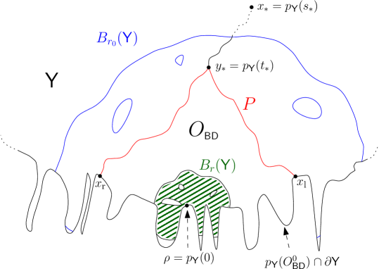
Figure 10: Proof of Theorem 3.7: The ball $B_{r}(\textup{{Y}})$ (shaded in green) itself is not simply connected, but it is included in a simply connected and open set $O_{\textup{{BD}}}\subset\textup{{Y}}$, which is homeomorphic to the closed half-plane $\overline{\mathbb{H}}$. The set $O_{\textup{{BD}}}$ is bordered by the simple curve $P$ (in red) in Y, which is the union of two geodesic segments starting from $x_{\textup{l}}$ and $x_{\textup{r}}$, respectively, and by the boundary segment $S=p_{\textup{{Y}}}(O_{\textup{{BD}}}^{0})\cap\partial\textup{{Y}}$. The larger ball $B_{r_{0}}(\textup{{Y}})$ encompasses $O_{\textup{{BD}}}$.

To finish the proof of Theorem 3.7, fix $r>0$, and let $a_{0}$ be large enough so that

$$\mathbb{P}\left(\min_{[0,a_{0}]}\gamma<-2r,\min_{[-a_{0},0]}\gamma<-2r\right)>1-\varepsilon/4\,.$$

Then, we choose $r_{0}>r$ such that, with $W^{\theta}$ the label function of $\textup{{BHP}}_{\theta}$,

$$\mathbb{P}(\omega(W^{\theta},[-\eta_{\textup{r}}(a_{0}),\eta_{\textup{l}}(a_{0})])\leq r_{0}/2)\geq 1-\varepsilon/4\,,$$

where $\omega(f,I)=\sup_{I}f-\inf_{I}f$ is the modulus of continuity of $f$ over the set $I$. We use this value of $r_{0}$ to apply Proposition 6.4. Fix $\varepsilon>0$. Then for every $T\geq T_{0}(\varepsilon/2)$ large enough, we can construct copies of $\textup{{Y}}=\textup{{BD}}_{T,\sigma(T)}$ and $\textup{{BHP}}_{\theta}$ such that $B_{r_{0}}(\textup{{Y}})$ and $B_{r_{0}}(\textup{{BHP}}_{\theta})$ are isometric with probability at least $1-\varepsilon/2$. More precisely, we are going to use the event $\mathcal{F}$ specified in the proof of Proposition 6.4 on which this property holds (in the definition of $\mathcal{F}$ we have to make sure that $A$ is chosen so that $A>a_{0}$), and which implies the property that $s_{\ast}\notin O^{0}_{\textup{{BD}}}$, on which our analysis so far is based. The probability of

$$\mathcal{F}^{\prime}=\mathcal{F}\cap\left\{\min_{[0,a_{0}]}\gamma<-2r,\min_{[-a_{0},0]}\gamma<-2r\right\}\cap\{\omega(W^{\theta},[-\eta_{\textup{r}}(a_{0}),\eta_{\textup{l}}(a_{0})])\leq r_{0}/2\}$$

is then at least $1-\varepsilon$. On this event we claim that

$$B_{r}(\textup{{Y}})\subset O_{\textup{{BD}}}\subset B_{r_{0}}(\textup{{Y}})\,.$$

The second inclusion comes from the fact that $D(0,s)\leq d_{W}(0,s)\leq 2\omega(W^{\theta},[-\eta_{\textup{r}}(a_{0}),\eta_{\textup{l}}(a_{0})])$ for every $s\in[0,\eta_{\textup{l}}(a_{0})]\cup[T-\eta_{\textup{r}}(a_{0}),T]$ (recall that $\mathbb{W}=W^{\theta}$ on the set $[-\eta_{\textup{r}}(A^{3}),\eta_{\textup{l}}(A^{3})]$ on $\mathcal{F}$). The first inclusion comes from the cactus bound, with the fact that $\min_{[0,a_{0}]}\gamma<-2r$ and $\min_{[-a_{0},0]}\gamma<-2r$, just as in the proof of (a) in Lemma 6.8. To be more precise, this shows that $B_{2r}(\textup{{Y}})\subset p_{\textup{{Y}}}([0,\eta_{\textup{l}}(a_{0})]\cup[T-\eta_{\textup{r}}(a_{0}),T])$, and since $O_{\textup{{BD}}}$ is equal to the interior of the latter set, the wanted inclusion follows. We refer to Figure 10 for an illustration.

Finally, we prove that $O_{\textup{{BHP}}}=I(O_{\textup{{BD}}})$ is an open subset of $\textup{{BHP}}_{\theta}$, where $I$ is the isometry defined before Corollary 6.10, or more precisely the induced map on Y. Let $x\in O_{\textup{{BHP}}}$, so that $x=I(y)$ for some $y\in O_{\textup{{BD}}}\subset B_{r_{0}}(\textup{{Y}})$. Let $\delta>0$ be such that $y+B_{\delta}(\textup{{Y}})\subset O_{\textup{{BD}}}$, and $x^{\prime}\in\textup{{BHP}}_{\theta}$ be such that $D_{\theta}(x,x^{\prime})<\delta$. Then $D_{\theta}(0,x^{\prime})\leq D_{\theta}(0,x)+\delta<r_{0}$, so that $x^{\prime}\in B_{r_{0}}(\textup{{BHP}}_{\theta})$. Therefore, there exists $y^{\prime}\in B_{r_{0}}(\textup{{Y}})$ with $x^{\prime}=I(y^{\prime})$, and one has $D(y,y^{\prime})=D_{\theta}(x,x^{\prime})<\delta$, so that $y^{\prime}\in O_{\textup{{BD}}}$, and thus $x^{\prime}\in O_{\textup{{BHP}}}$. This proves that $O_{\textup{{BHP}}}$ is open and concludes the proof of Theorem 3.7.

6.3 Coupling quadrangulations of large volumes (Propositions 3.11 and 3.14)

We begin with the proof of Proposition 3.11, which is in spirit of [19, Lemma 8 and Proposition 9].

Proof of Proposition 3.11.

Assume $1\ll\sigma_{n}\ll n$. Set $\vartheta_{n}=\min\{\sigma_{n},\,n/\sigma_{n}\}$, and let $\varepsilon>0$. Let $((\textup{$\mathfrak{f}$}_{n},\textup{$\mathfrak{l}$}_{n}),\textup{{b}}_{n})$ be uniformly distributed over the set $\textup{$\mathfrak{F}$}_{\sigma_{n}}^{n}\times\textup{$\mathfrak{B}$}_{\sigma_{n}}$, and consider a triplet $((\textup{$\mathfrak{f}$}_{\infty},\textup{$\mathfrak{l}$}_{\infty}),\textup{{b}}_{\infty})$ of a uniformly labeled critical infinite forest and a uniform infinite bridge.

We first argue that we can find $\delta>0$ and $n_{0}$ such that for all $n\geq n_{0}$, we can construct $((\textup{$\mathfrak{f}$}_{n},\textup{$\mathfrak{l}$}_{n}),\textup{{b}}_{n})$ and $((\textup{$\mathfrak{f}$}_{\infty},\textup{$\mathfrak{l}$}_{\infty}),\textup{{b}}_{\infty})$ on the same probability space such that on an event of probability at least $1-\varepsilon$, the corresponding balls of radius $2\delta\sqrt{\vartheta_{n}}$ around the vertices $\textup{$\mathfrak{f}$}_{n}(0)$ and $\textup{$\mathfrak{f}$}_{\infty}(0)$ in the associated quadrangulations are isometric.

For $0\leq k\leq\sigma_{n}-1$, write $\tau(\textup{$\mathfrak{f}$}_{n},k)$ for the tree of $\textup{$\mathfrak{f}$}_{n}$ rooted at $(k)$, and put $\tau(\textup{$\mathfrak{f}$}_{n},\sigma_{n})=\tau(\textup{$\mathfrak{f}$}_{n},0)$. Similarly, define $\tau(\textup{$\mathfrak{f}$}_{\infty},k)$ to be the tree of $\textup{$\mathfrak{f}$}_{\infty}$ rooted at $(k)$, where now $k\in\mathbb{Z}$.

As a consequence of Lemmas 5.3 and 5.5, there exist $\delta^{\prime}>0$ and $n^{\prime}_{0}\in\mathbb{N}$ such that for $n\geq n^{\prime}_{0}$, with $A_{n}=\lfloor\delta^{\prime}\vartheta_{n}\rfloor$, we can construct $((\textup{$\mathfrak{f}$}_{n},\textup{$\mathfrak{l}$}_{n}),\textup{{b}}_{n})$ and $((\textup{$\mathfrak{f}$}_{\infty},\textup{$\mathfrak{l}$}_{\infty}),\textup{{b}}_{\infty})$ on the same probability space such that if we let

$$\mathcal{E}^{1}(n,\delta^{\prime}) =\quad\left\{\tau(\textup{$\mathfrak{f}$}_{n},i)=\tau(\textup{$\mathfrak{f}$}_{\infty},i),\,\tau(\textup{$\mathfrak{f}$}_{n},\sigma_{n}-i)=\tau(\textup{$\mathfrak{f}$}_{\infty},-i),\,0\leq i\leq A_{n}\right\}$$

$$\,\quad\cap\left\{\textup{{b}}_{n}(i)=\textup{{b}}_{\infty}(i),\,\textup{{b}}_{n}(\sigma_{n}-i)=\textup{{b}}_{\infty}(-i),\,1\leq i\leq A_{n}\right\}$$

$$\,\quad\cap\left\{\textup{$\mathfrak{l}$}_{n}|_{\tau(\textup{$\mathfrak{f}$}_{n},i)}=\textup{$\mathfrak{l}$}_{\infty}|_{\tau(\textup{$\mathfrak{f}$}_{\infty},i)},\,\textup{$\mathfrak{l}$}_{n}|_{\tau(\textup{$\mathfrak{f}$}_{n},\sigma_{n}-i)}=\textup{$\mathfrak{l}$}_{\infty}|_{\tau(\textup{$\mathfrak{f}$}_{\infty},-i)},\,0\leq i\leq A_{n}\right\},$$

then $\mathcal{E}^{1}(n,\delta^{\prime})$ has probability at least $1-\varepsilon/3$. We fix such a $\delta^{\prime}$. For $\delta>0$ and $n\in\mathbb{N}$, put

$$\mathcal{E}^{2}(n,\delta)=\left\{\min_{[0,\,A_{n}]}\textup{{b}}_{\infty}<-5\delta\sqrt{\vartheta_{n}},\,\min_{[-A_{n},\,0]}\textup{{b}}_{\infty}<-5\delta\sqrt{\vartheta_{n}}\right\}\cap\left\{-\textup{{b}}_{\infty}(-1)<\delta^{-1}\right\},$$

and let

$$\mathcal{E}^{3}(n,\delta)=\left\{\min_{[A_{n}+1,\,\sigma_{n}-(A_{n}+1)]}\textup{{b}}_{n}<-5\delta\sqrt{\vartheta_{n}}\right\}.$$

Donsker’s invariance principle applied to $(\textup{{b}}_{\infty}(i),i\in\mathbb{Z})$ guarantees that we can find $\delta>0$ such that for all sufficiently large $n$,

$$\mathbb{P}\left(\mathcal{E}^{2}(n,\delta)\right)\geq 1-\varepsilon/3.$$

Moreover, provided $n$ is large enough and $\delta>0$ is sufficiently small, Lemma 5.4 ensures that

$$\mathbb{P}\left(\mathcal{E}^{3}(n,\delta)\right)\geq 1-\varepsilon/3.$$

We fix $n_{0}\geq n^{\prime}_{0}$ and $\delta>0$ such that for all $n\geq n_{0}$, the bounds in the last two displays hold.

From now on, we work on the event $\mathcal{E}^{1}(n,\delta^{\prime})\cap\mathcal{E}^{2}(n,\delta)\cap\mathcal{E}^{3}(n,\delta)$. Let $(Q_{n}^{\sigma_{n}},v^{\bullet})=\Phi_{n}(((\textup{$\mathfrak{f}$}_{n},\textup{$\mathfrak{l}$}_{n}),\textup{{b}}_{n}))$ and $Q_{\infty}^{\infty}=\Phi_{\infty}(((\textup{$\mathfrak{f}$}_{\infty},\textup{$\mathfrak{l}$}_{\infty}),\textup{{b}}_{\infty}))$ be the quadrangulations constructed from the triplets $((\textup{$\mathfrak{f}$}_{n},\textup{$\mathfrak{l}$}_{n}),\textup{{b}}_{n})$ and $((\textup{$\mathfrak{f}$}_{\infty},\textup{$\mathfrak{l}$}_{\infty}),\textup{{b}}_{\infty})$ via the Bouttier-Di Francesco-Guitter mapping. We denote by $d_{n}$ and $d_{\infty}$ the graph distances on $V(Q_{n}^{\sigma_{n}})$ and $V(Q_{\infty}^{\infty})$. We write

$$\textup{$\mathfrak{f}$}^{\prime}_{n}=\left(\tau(\textup{$\mathfrak{f}$}_{n},\sigma_{n}-A_{n}),\ldots,\tau(\textup{$\mathfrak{f}$}_{n},\sigma_{n}-1),\tau(\textup{$\mathfrak{f}$}_{n},0),\ldots,\tau(\textup{$\mathfrak{f}$}_{n},A_{n})\right)$$

for the forest obtained from restricting $\textup{$\mathfrak{f}$}_{n}$ to the last $A_{n}$ and the first $A_{n}+1$ trees, and identically

$$\textup{$\mathfrak{f}$}^{\prime}_{\infty}=\left(\tau(\textup{$\mathfrak{f}$}_{\infty},-A_{n}),\ldots,\tau(\textup{$\mathfrak{f}$}_{\infty},-1),\tau(\textup{$\mathfrak{f}$}_{\infty},0),\ldots,\tau(\textup{$\mathfrak{f}$}_{\infty},A_{n})\right).$$

Recall the cactus bounds (4.3) and (4.6) for $Q_{n}^{\sigma_{n}}$ and $Q_{\infty}^{\infty}$, respectively. For vertices $v\in V(\textup{$\mathfrak{f}$}_{n})\setminus V(\textup{$\mathfrak{f}$}^{\prime}_{n})$, we obtain, with $(0)=\textup{$\mathfrak{f}$}_{n}(0)$,

$$d_{n}((0),v)\geq-\max\left\{\min_{[0,A_{n}]}\textup{{b}}_{n},\min_{[-A_{n},0]}\textup{{b}}_{n}\right\}\geq 5\delta\sqrt{\vartheta_{n}},$$

and identically, for vertices $v\in V(\textup{$\mathfrak{f}$}_{\infty})\setminus V(\textup{$\mathfrak{f}$}^{\prime}_{\infty})$, writing now $(0)$ for $\textup{$\mathfrak{f}$}_{\infty}(0)$, $d_{\infty}((0),v)\geq 5\delta\sqrt{\vartheta_{n}}.$ We argue now similarly to the second part in the proof of [19, Lemma 8]. Firstly, if $u\in V(\textup{$\mathfrak{f}$}_{n})$ is any vertex with $d_{n}((0),u)\leq 5\delta\sqrt{\vartheta_{n}}-1$, then any vertex on a geodesic path from $(0)$ to $u$ in $Q_{n}^{\sigma_{n}}$ satisfies the same bound and must therefore belong to one of the trees in $\textup{$\mathfrak{f}$}^{\prime}_{n}$. From the construction of edges in the Bouttier-Di Francesco-Guitter mapping, we deduce that any edge of $Q_{n}^{\sigma_{n}}$ on such a geodesic path corresponds to an edge of $Q_{\infty}^{\infty}$ with the same endpoints, provided none of these edges in $Q_{n}^{\sigma_{n}}$ connect two vertices $w$ and $w^{\prime}$ such that the set of vertices between $w$ and $w^{\prime}$ in the cyclic contour order around the forest $\textup{$\mathfrak{f}$}_{n}$ contains the vertices of $\textup{$\mathfrak{f}$}_{n}\setminus\textup{$\mathfrak{f}$}_{n}^{\prime}$. But on the event $\mathcal{E}^{3}(n,\delta)$, the set of vertices between $w$ and $w^{\prime}$ would in particular contain a (root) vertex of $\textup{$\mathfrak{f}$}_{n}\setminus\textup{$\mathfrak{f}$}_{n}^{\prime}$ with label less than $-5\delta\sqrt{\vartheta_{n}}$. This would imply that both vertices $w$ and $w^{\prime}$ of such an edge have a label which is smaller than $-5\delta\sqrt{\vartheta_{n}}$, too, in contradiction to the fact that $d_{n}((0),v)\leq 5\delta\sqrt{\vartheta_{n}}-1$ for all vertices $v$ on a geodesic between $(0)$ and $u$. We deduce that if $u\in V(\textup{$\mathfrak{f}$}_{n})$ satisfies $d_{n}((0),u)\leq 5\delta\sqrt{\vartheta_{n}}-1$, then $d_{\infty}((0),u)\leq d_{n}((0),u)$. Since in turn any edge of $Q_{\infty}^{\infty}$ on a geodesic between $(0)$ and a vertex $u\in V(\textup{$\mathfrak{f}$}_{\infty})$ with $d_{\infty}((0),u)\leq 5\delta\sqrt{\vartheta_{n}}-1$ does correspond to an edge of $Q_{n}^{\sigma_{n}}$ with the same endpoints, we obtain also $d_{n}((0),u)\leq d_{\infty}((0),u)$. Therefore, we have that vertices with distance at most $5\delta\sqrt{\vartheta_{n}}-1$ from $(0)$ are the same in $Q_{n}^{\sigma_{n}}$ and $Q_{\infty}^{\infty}$. We claim that

$$d_{n}(u,v)=d_{\infty}(u,v)\quad\hbox{whenever }u,v\in B^{(0)}_{2\delta\sqrt{\vartheta_{n}}}(Q_{n}^{\sigma_{n}}).$$ (6.25)

Indeed, if $u,v$ are vertices in $B^{(0)}_{2\delta\sqrt{\vartheta_{n}}}(Q_{n}^{\sigma_{n}})$, then any geodesic connecting $u$ to $v$ in $Q_{n}^{\sigma_{n}}$ must lie entirely in $B^{(0)}_{4\delta\sqrt{\vartheta_{n}}}(Q_{n}^{\sigma_{n}})$, and any edge on such a geodesic corresponds to an edge in $Q_{\infty}^{\infty}$. Since the converse is also true, we obtain (6.25), and with the correspondence of edges between $Q_{n}^{\sigma_{n}}$ and $Q_{\infty}^{\infty}$ alluded to above we deduce that the balls $B^{(0)}_{2\delta\sqrt{\vartheta_{n}}}(Q_{n}^{\sigma_{n}})$ and $B^{(0)}_{2\delta\sqrt{\vartheta_{n}}}(Q_{\infty}^{\infty})$ are isometric on an event of probability at least $1-\varepsilon$.

Finally, recall from the Bouttier-Di Francesco-Guitter bijection that the root vertex $\rho_{n}$ of $Q_{n}^{\sigma_{n}}$ is given by $\textup{$\mathfrak{f}$}_{n}(\textup{succ}^{-\textup{{b}}_{n}(\sigma_{n})}(0))$, where conditionally on $\textup{{b}}_{n}(\sigma_{n}-1)$, $\textup{{b}}_{n}(\sigma_{n})$ is uniformly distributed on $\{\textup{{b}}_{n}(\sigma_{n}-1)-1,\ldots,0\}$. Similarly, the root vertex $\rho$ of $Q_{\infty}^{\infty}$ is given by $\textup{$\mathfrak{f}$}_{\infty}(\textup{succ}^{-\textup{{b}}_{\infty}(\partial)}(0))$, where conditionally on $\textup{{b}}_{\infty}(-1)$, $\textup{{b}}_{\infty}(\partial)$ is uniformly distributed on $\{\textup{{b}}_{\infty}(-1)-1,\ldots,0\}$. On the event $\mathcal{E}^{1}(n,\delta^{\prime})\cap\mathcal{E}^{2}(n,\delta)$, we can couple $\textup{{b}}_{n}(\sigma_{n})$ and $\textup{{b}}_{\infty}(\partial)$ such that $\textup{{b}}_{n}(\sigma_{n})=\textup{{b}}_{\infty}(\partial)$. Moreover, for $n$ large enough, we have on this event $B_{\delta\sqrt{\vartheta_{n}}}(Q_{n}^{\sigma_{n}})\subset B^{(0)}_{2\delta\sqrt{\vartheta_{n}}}(Q_{n}^{\sigma_{n}})$ and $B_{\delta\sqrt{\vartheta_{n}}}(Q_{\infty}^{\infty})\subset B_{2\delta\sqrt{\vartheta_{n}}}^{(0)}(Q_{\infty}^{\infty})$. Therefore, we have equality of $B_{\delta\sqrt{\vartheta_{n}}}(Q_{n}^{\sigma_{n}})$ and $B_{\delta\sqrt{\vartheta_{n}}}(Q_{\infty}^{\infty})$ on the event $\mathcal{E}^{1}(n,\delta^{\prime})\cap\mathcal{E}^{2}(n,\delta)\cap\mathcal{E}^{3}(n,\delta)$. Local convergence of $Q_{n}^{\sigma_{n}}$ towards UIHPQ in the sense of $d_{\textup{map}}$ is a direct consequence of this, and the proposition is proved. ∎

We now turn to the proof of Proposition 3.14. We will adopt the notion of [19, Section 4.3.1] concerning pruned (pointed) trees. More precisely, a (finite) pointed tree consists of a pair $\boldsymbol{\tau}=(\tau,\xi)$, where $\tau$ is a tree of finite size and $\xi$ is a distinguished vertex of $\tau$. Given such a pointed tree $\boldsymbol{\tau}=(\tau,\xi)$ and $h$ an integer with $0\leq h<|\xi|$, $\mathscr{P}(\boldsymbol{\tau},h)$ represents the subtree of $\tau$ containing all the vertices $u\in V(\tau)$ such that the height of the most recent common ancestor of $u$ and $\xi$ is strictly less than $h$, together with the ancestor $\left[\xi\right]_{h}$ of $\xi$ at height exactly $h$. By pointing $\mathscr{P}(\boldsymbol{\tau},h)$ at $\left[\xi\right]_{h}$, this subtree is itself considered as a pointed tree. If $h\geq|\xi|$, we agree that $\mathscr{P}(\boldsymbol{\tau},h)=(\{\emptyset\},\emptyset)$, where $\emptyset$ represents the root vertex of $\tau$. It is straightforward to see that if $\boldsymbol{\tau}=(\tau,\xi)$ is a pointed tree and $h$ and $h^{\prime}$ are two integers with $h^{\prime}\geq h\geq 0$, then

$$\mathscr{P}\left((\boldsymbol{\tau},h^{\prime}),h\right)=\mathscr{P}\left(\boldsymbol{\tau},h\right).$$ (6.26)

Proof of Proposition 3.14.

We assume $1\ll\sigma_{n}\ll\sqrt{n}$ and fix $\varepsilon>0$ and $r>0$ for the rest of this proof. We let $((\textup{$\mathfrak{f}$}_{n},\textup{$\mathfrak{l}$}_{n}),\textup{{b}}_{n})$ be uniformly distributed over the set $\textup{$\mathfrak{F}$}_{\sigma_{n}}^{n}\times\textup{$\mathfrak{B}$}_{\sigma_{n}}$, and for given $R\in\mathbb{N}$, we let $((\textup{$\mathfrak{f}$}^{\prime}_{n},\textup{$\mathfrak{l}$}^{\prime}_{n}),\textup{{b}}^{\prime}_{n})$ be uniformly distributed over $\textup{$\mathfrak{F}$}_{\sigma_{n}}^{R\sigma_{n}^{2}}\times\textup{$\mathfrak{B}$}_{\sigma_{n}}$. Identically to the proof of Proposition 3.11, it suffices to show that we can find $R_{0}>0$ and $n_{0}\in\mathbb{N}$ such that for all integers $R\geq R_{0}$ and all $n\geq n_{0}$, we can construct $((\textup{$\mathfrak{f}$}_{n},\textup{$\mathfrak{l}$}_{n}),\textup{{b}}_{n})$ and $((\textup{$\mathfrak{f}$}^{\prime}_{n},\textup{$\mathfrak{l}$}^{\prime}_{n}),\textup{{b}}^{\prime}_{n})$ on the same probability space such that on an event of probability at least $1-\varepsilon$, the corresponding balls of radius $2r\sqrt{\sigma_{n}}$ around the vertices $\textup{$\mathfrak{f}$}_{n}(0)$ and $\textup{$\mathfrak{f}$}^{\prime}_{n}(0)$ in the associated quadrangulations are isometric.

For $0\leq k\leq\sigma_{n}-1$, we let $\tau(\textup{$\mathfrak{f}$}_{n},k)$ be the tree of $\textup{$\mathfrak{f}$}_{n}$ rooted at $(k)$ and denote by $i_{\ast}$ the smallest index such that $|\tau(\textup{$\mathfrak{f}$}_{n},i_{\ast})|\geq|\tau(\textup{$\mathfrak{f}$}_{n},k)|$ for all $0\leq k\leq\sigma_{n}-1$. We shall point the tree $\tau(\textup{$\mathfrak{f}$}_{n},i_{\ast})$, by choosing conditionally on $\tau(\textup{$\mathfrak{f}$}_{n},i_{\ast})$ a vertex $\xi_{n}\in V(\tau(\textup{$\mathfrak{f}$}_{n},i_{\ast}))$ uniformly at random. We write $(\tau(\textup{$\mathfrak{f}$}_{n},i_{\ast}),\xi_{n})$ for the pointed tree obtained in this way, and for $h\in\mathbb{N}$, we write $\textup{$\mathfrak{l}$}_{n}|_{\mathscr{P}((\tau(\textup{$\mathfrak{f}$}_{n},i_{\ast}),\xi_{n}),h)}$ for the restriction of the labels $\textup{$\mathfrak{l}$}_{n}$ of $\textup{$\mathfrak{f}$}_{n}$ to the subtree $\mathscr{P}((\tau(\textup{$\mathfrak{f}$}_{n},i_{\ast}),\xi_{n}),h)$ of $(\tau(\textup{$\mathfrak{f}$}_{n},i_{\ast}),\xi_{n})$ pruned at height $h$, see the notation above. Finally, we let $(\tau_{i},\ell_{i})$, $0\leq i\leq\sigma_{n}-1$, be a sequence of independent uniformly labeled critical geometric Galton-Watson trees.

For $H\in\mathbb{N}$, set $H_{n}=H\sigma_{n}$. Recall that the law of $((\textup{$\mathfrak{f}$}^{\prime}_{n},\textup{$\mathfrak{l}$}^{\prime}_{n}),\textup{{b}}^{\prime}_{n})$ depends on $R\in\mathbb{N}$. We claim that for each fixed integer $H\in\mathbb{N}$, provided $n$ and $R$ are sufficiently large, we can construct $((\textup{$\mathfrak{f}$}_{n},\textup{$\mathfrak{l}$}_{n}),\textup{{b}}_{n})$, $((\textup{$\mathfrak{f}$}^{\prime}_{n},\textup{$\mathfrak{l}$}^{\prime}_{n}),\textup{{b}}^{\prime}_{n})$, $\xi_{n}$, $\xi^{\prime}_{n}$ and $(\tau_{i},\ell_{i})$ for $0\leq i\leq\sigma_{n}-1$ on the same probability space such that the event

$$\mathcal{E}_{1}(n,R,H) =\left\{i_{\ast}=i^{\prime}_{\ast}\right\}\cap\left\{\tau(\textup{$\mathfrak{f}$}_{n},i)=\tau(\textup{$\mathfrak{f}$}^{\prime}_{n},i)=\tau_{i},\,0\leq i\leq\sigma_{n}-1,\,i\neq i_{\ast}\right\}$$

$$\,\quad\cap\left\{\mathscr{P}\left((\tau(\textup{$\mathfrak{f}$}_{n},i_{\ast}),\xi_{n}),H_{n}\right)=\mathscr{P}\left((\tau(\textup{$\mathfrak{f}$}^{\prime}_{n},i^{\prime}_{\ast}),\xi^{\prime}_{n}),H_{n}\right)\neq(\{\emptyset\},\emptyset)\right\}$$

$$\,\quad\cap\left\{\textup{{b}}_{n}(i)=\textup{{b}}^{\prime}_{n}(i),\,0\leq i\leq\sigma_{n}\right\}$$

$$\,\quad\cap\left\{\textup{$\mathfrak{l}$}_{n}|_{\tau(\textup{$\mathfrak{f}$}_{n},i)}=\textup{$\mathfrak{l}$}^{\prime}_{n}|_{\tau(\textup{$\mathfrak{f}$}^{\prime}_{n},i)}=\ell_{i},\,0\leq i\leq\sigma_{n}-1,i\neq i_{\ast}\right\}$$

$$\,\quad\cap\left\{\textup{$\mathfrak{l}$}_{n}|_{\mathscr{P}\left((\tau(\textup{$\mathfrak{f}$}_{n},i_{\ast}),\xi_{n}),H_{n}\right)}=\textup{$\mathfrak{l}$}^{\prime}_{n}|_{\mathscr{P}\left((\tau(\textup{$\mathfrak{f}$}^{\prime}_{n},i^{\prime}_{\ast}),\xi^{\prime}_{n}),H_{n}\right)}\right\}$$

has probability at least $1-\varepsilon/2$. Let us look separately at the different sets on the right hand side. Firstly, from Lemma 5.1 we know that $\textup{$\mathfrak{f}$}_{n}$ has with high probability a unique largest tree of order $\sigma_{n}^{2}$, and its index is uniform in $\{0,\ldots,\sigma_{n}-1\}$. Moreover, Lemma 5.2 asserts that the other trees of $\textup{$\mathfrak{f}$}_{n}$ are close in total variation to $\sigma_{n}-1$ critical geometric Galton-Watson trees. The same holds for $\textup{$\mathfrak{f}$}^{\prime}_{n}$, from which we deduce that $\textup{$\mathfrak{f}$}_{n},\textup{$\mathfrak{f}$}^{\prime}_{n}$ and $\tau_{i}$, $0\leq i\leq\sigma_{n}-1$, can be coupled such that the intersection of the first two events on the right hand side has probability at least $1-\varepsilon/3$, say. For the event on the second line concerning the pruned trees, we use that fact that conditionally on $|\tau(\textup{$\mathfrak{f}$}_{n},i_{\ast})|=m_{n}$, $(\tau(\textup{$\mathfrak{f}$}_{n},i_{\ast}),\xi_{n})$ is uniformly distributed over the set of all pointed trees of size $m_{n}$. A similar statement holds for $\tau(\textup{$\mathfrak{f}$}^{\prime}_{n},i^{\prime}_{\ast})$. Now by Lemma 5.1, for any $K>0$, the probability that $|\tau(\textup{$\mathfrak{f}$}_{n},i_{\ast})|\geq K\sigma^{2}_{n}$ tends to one with increasing $n$, since $n\gg\sigma_{n}^{2}$. Similarly, for any given $K>0$, by choosing $R$ large enough, we can ensure that $|\tau(\textup{$\mathfrak{f}$}^{\prime}_{n},i^{\prime}_{\ast})|\geq K\sigma^{2}_{n}$ holds with a probability as close to one as we wish for large $n$. An application of Proposition $7$ of [19] therefore shows that both $\mathscr{P}\left((\tau(\textup{$\mathfrak{f}$}_{n},i_{\ast}),\xi_{n}),H_{n}\right)$ and $\mathscr{P}\left((\tau(\textup{$\mathfrak{f}$}^{\prime}_{n},i^{\prime}_{\ast}),\xi^{\prime}_{n}),H_{n}\right)$ are for large $R$ and $n$ close in total variation to the so-called uniform infinite tree (or Kesten’s tree) pruned at height $H_{n}$. Applying the triangle inequality, we see that the total variation distance between $\mathscr{P}\left((\tau(\textup{$\mathfrak{f}$}_{n},i_{\ast}),\xi_{n}),H_{n}\right)$ and $\mathscr{P}\left((\tau(\textup{$\mathfrak{f}$}^{\prime}_{n},i^{\prime}_{\ast}),\xi^{\prime}_{n}),H_{n}\right)$ can be made as small as we wish, provided $R$ and $n$ are taken sufficiently large.

Combining the above coupling with this last observation, we infer that we can in fact couple $\textup{$\mathfrak{f}$}_{n}$, $\textup{$\mathfrak{f}$}^{\prime}_{n}$, $\xi_{n}$, $\xi_{n}^{\prime}$ and $\tau_{i}$ for $0\leq i\leq\sigma_{n}-1$ such that the intersection of the first three events on the right hand side has probability at least $1-\varepsilon/2$ for large $R$ and $n$. Since the bridges $\textup{{b}}_{n}$ and $\textup{{b}}^{\prime}_{n}$ have both the same law and are independent of the trees, we can additionally assume that the probability space carries realizations of $\textup{{b}}_{n}$ and $\textup{{b}}^{\prime}_{n}$ such that $\textup{{b}}_{n}\equiv\textup{{b}}^{\prime}_{n}$. A similar arguments allows us to couple the labelings $\textup{$\mathfrak{l}$}_{n}$, $\textup{$\mathfrak{l}$}^{\prime}_{n}$, and $\ell_{i}$ such that the last two events on the right hand side in the definition of $\mathcal{E}_{1}(n,R,H)$ hold true. This proves the claim about $\mathcal{E}_{1}(n,R,H)$.

We will now work on the event $\mathcal{E}_{1}(n,R,H)$ and let $(Q_{n}^{\sigma_{n}},v^{\bullet})=\Phi_{n}(((\textup{$\mathfrak{f}$}_{n},\textup{$\mathfrak{l}$}_{n}),\textup{{b}}_{n}))$ and $(Q_{R\sigma_{n}^{2}}^{\sigma_{n}},w^{\bullet})=\Phi_{R\sigma_{n}^{2}}(((\textup{$\mathfrak{f}$}^{\prime}_{n},\textup{$\mathfrak{l}$}^{\prime}_{n}),\textup{{b}}^{\prime}_{n}))$ be the quadrangulations constructed from the triplets $((\textup{$\mathfrak{f}$}_{n},\textup{$\mathfrak{l}$}_{n}),\textup{{b}}_{n})$ and $((\textup{$\mathfrak{f}$}^{\prime}_{n},\textup{$\mathfrak{l}$}^{\prime}_{n}),\textup{{b}}^{\prime}_{n})$, respectively. Recall that $[\xi_{n}]_{H_{n}}$ denotes the ancestor of $\xi_{n}$ in $\tau(\textup{$\mathfrak{f}$}_{n},i_{\ast})$ at height $H_{n}$. Let

$$M_{n}=-\min_{[[\emptyset,[\xi_{n}]_{H_{n}}]]}\textup{$\mathfrak{l}$}_{n},$$

where $[[\emptyset,[\xi_{n}]_{H_{n}}]]$ is the vertex set of the unique injective path in $\tau(\textup{$\mathfrak{f}$}_{n},i_{\ast})$ connecting the (tree) root $\emptyset$ to $[\xi_{n}]_{H_{n}}$. By definition of the labeling $\textup{$\mathfrak{l}$}_{n}$, conditionally on the tree, $M_{n}$ has the law of the maximum attained by a random walk started at zero and stopped after $H_{n}$ many steps, with increments uniformly distributed in $\{-1,0,1\}$. Setting

$$\mathcal{E}_{2}(n,H)=\left\{M_{n}\geq 5r\sqrt{\sigma_{n}}\right\},$$

we can ensure by an application of Donsker’s invariance principle that for $H\in\mathbb{N}$ sufficiently large (recall that $r$ was fixed at the beginning, and $H_{n}=H\sigma_{n}$), the event $\mathcal{E}_{2}(n,H)$ has probability at least $1-\varepsilon/2$. In particular, by choosing $H\in\mathbb{N}$ large enough, we obtain that $\mathcal{E}_{1}(n,R,H)\cap\mathcal{E}_{2}(n,H)$ has probability at least $1-\varepsilon$ for all $R$, $n\in\mathbb{N}$ sufficiently large.

It remains to convince ourselves that on the event $\mathcal{E}_{1}(n,R,H)\cap\mathcal{E}_{2}(n,H)$, the balls $B^{(0)}_{2r\sqrt{\sigma_{n}}}(Q_{n}^{\sigma_{n}})$ and $B^{(0)}_{2r\sqrt{\sigma_{n}}}(Q_{R\sigma_{n}^{2}}^{\sigma_{n}})$ are isometric. Since the arguments are very close to those provided in the proofs of Proposition 3.11 above and [19, Lemma 8], we only sketch them in order to avoid too much repetition. Write $\emptyset=u_{0},u_{1},\ldots,u_{H_{n}}=[\xi_{n}]_{H_{n}}$ for the vertices of the non-backtracking path connecting $\emptyset$ to $[\xi_{n}]_{H_{n}}$ in $\tau(\textup{$\mathfrak{f}$}_{n},i_{\ast})$. Let $k_{n}\in\{0,\ldots,H_{n}\}$ such that

$$\textup{$\mathfrak{l}$}_{n}(u_{k_{n}})=-\min_{[[\emptyset,[\xi_{n}]_{H_{n}}]]}\textup{$\mathfrak{l}$}_{n}.$$

Recall the identification of $V(Q_{n}^{\sigma_{n}})\setminus\{v^{\bullet}\}$ with $V(\textup{$\mathfrak{f}$}_{n})$. Denote by $d_{n}$ the graph distance on $V(Q_{n}^{\sigma_{n}})$. If $v$ is a vertex of $\tau(\textup{$\mathfrak{f}$}_{n},i_{\ast})$ that does not belong to the subtree $\mathscr{P}\left((\tau(\textup{$\mathfrak{f}$}_{n},i_{\ast}),\xi_{n}),k_{n}\right)$, then the ancestral lines of $v$ and $\xi_{n}$ coincide at least up to level $k_{n}$. In particular, they both contain the vertex $u_{k_{n}}$. For such vertices $v$, we obtain from the cactus bound (4.3) on the event $\mathcal{E}_{1}(n,R,H)\cap\mathcal{E}_{2}(n,H)$ the bound

$$d_{n}((0),v)\geq 5r\sqrt{\sigma_{n}},$$

with $(0)=\textup{$\mathfrak{f}$}_{n}(0)$. See [19, Proof of Lemma 8] for the complete argument (note however that $(0)$ might be the root of a tree different from $\tau(\textup{$\mathfrak{f}$}_{n},i_{\ast})$). On $\mathcal{E}_{1}(n,R,H)$, using additionally (6.26),

$$\mathscr{P}\left((\tau(\textup{$\mathfrak{f}$}_{n},i_{\ast}),\xi_{n}),k_{n}\right)=\mathscr{P}\left((\tau(\textup{$\mathfrak{f}$}^{\prime}_{n},i^{\prime}_{\ast}),\xi^{\prime}_{n}),k_{n}\right),$$

and the labelings $\textup{$\mathfrak{l}$}_{n}$ and $\textup{$\mathfrak{l}$}^{\prime}_{n}$ restricted to the subtrees on the left and right, respectively, agree. Therefore, a similar inequality holds for $Q_{R\sigma^{2}_{n}}^{\sigma_{n}}$, for vertices $v^{\prime}$ of $\tau(\textup{$\mathfrak{f}$}^{\prime}_{n},i^{\prime}_{\ast}))$ which do not belong to the subtree $\mathscr{P}\left((\tau(\textup{$\mathfrak{f}$}^{\prime}_{n},i^{\prime}_{\ast}),\xi^{\prime}_{n}),k_{n}\right)$. Adapting now the reasoning of [19, Proof of Lemma 8] to our situation (see also the proof of Proposition 3.11 above), we obtain that vertices with distance at most $5r\sqrt{\sigma_{n}}-1$ from $(0)$ are the same in $Q_{n}^{\sigma_{n}}$ and $Q_{R\sigma^{2}_{n}}^{\sigma_{n}}$ on the event $\mathcal{E}_{1}(n,R,H)\cap\mathcal{E}_{2}(n,H)$, and, with $d_{n}^{\prime}$ being the graph distance in $Q_{R\sigma^{2}_{n}}^{\sigma_{n}}$,

$$d_{n}(u,v)=d^{\prime}_{n}(u,v)\quad\hbox{whenever }u,v\in B^{(0)}_{2r\sqrt{\sigma_{n}}}(Q_{n}^{\sigma_{n}}).$$

This finishes our proof. ∎

6.4 Brownian half-plane with zero skewness (Theorems 3.3 and 3.6)

We work in the usual setting from Section 4.5.4. In particular, $Q_{n}^{\sigma_{n}}$ denotes a random variable with the uniform distribution over the set $\mathcal{Q}_{n}^{\sigma_{n}}$ of rooted quadrangulations with $n$ internal faces and $2\sigma_{n}$ boundary edges.

Our proofs of Theorems 3.3 and 3.6 are essentially consequences of the coupling of balls between the Brownian disk $\textup{{BD}}_{T,\sqrt{T}}$ and the Brownian half-plane BHP (Proposition 6.4), of the fundamental convergence

$$\left(V(Q_{n}^{\sigma_{n}}),(8/9)^{-1/4}n^{-1/4}d_{\textup{gr}},\rho_{n}\right)\xrightarrow[n\to\infty]{(d)}\textup{{BD}}_{\sigma}=\textup{{BD}}_{1,\sigma}$$ (6.27)

proved in [9, Theorem 1] for the regime $\sigma_{n}\sim\sigma\sqrt{2n}$ when $\sigma\in(0,\infty)$ is a fixed real and of the coupling between $Q_{n}^{\sigma_{n}}$ and the UIHPQ $Q_{\infty}^{\infty}$ (Proposition 3.11).

Proof of Theorem 3.6.

In view of Remark 2.10, the result follows if we show that for every $r\geq 0$ and every sequence of positive reals $a_{n}\rightarrow\infty$,

$$B_{r}\left(a_{n}^{-1}\cdot Q_{\infty}^{\infty}\right)\xrightarrow[n\to\infty]{(d)}B_{r}(\textup{{BHP}})$$

in distribution in $\mathbb{K}$. For notational simplicity, we restrict ourselves to the case $r=1$. Fix $\varepsilon>0$. By Proposition 6.4, we find $T_{0}=T_{0}(\varepsilon)>0$ such that for all $T\geq T_{0}$, we can construct copies of $\textup{{BD}}_{T,\sqrt{T}}$ and BHP on the same probability space such that

$$B_{1}\left(\textup{{BD}}_{T,\sqrt{T}}\right)=B_{1}(\textup{{BHP}})$$ (6.28)

with probability at least $1-\varepsilon$.

Let $\sigma_{n}=\lceil\sqrt{2n}\rceil$. By Proposition 3.11, there exists $\delta>0$ such that for $n$ large enough, we can couple $Q_{n}^{\sigma_{n}}$ and $Q_{\infty}^{\infty}$ on the same probability space such that with probability at least $1-\varepsilon$, $B_{\delta\sqrt{\sigma_{n}}}\left(Q_{n}^{\sigma_{n}}\right)=B_{\delta\sqrt{\sigma_{n}}}\left(Q_{\infty}^{\infty}\right).$ We can and will assume that $\delta<2T_{0}^{-1/4}$. We put $m_{n}=\lceil\delta^{-4}a_{n}^{4}\rceil$. Then $a_{n}\leq\delta\sqrt{\sigma_{m_{n}}}$. With $m_{n}$ taking the role of $n$, the last observation enables us to find a coupling between $Q_{m_{n}}^{\sigma_{m_{n}}}$ and $Q_{\infty}^{\infty}$ on the same probability space such that for large $n$, we have with probability at least $1-\varepsilon$

$$B_{a_{n}}\left(Q_{m_{n}}^{\sigma_{m_{n}}}\right)=B_{a_{n}}\left(Q_{\infty}^{\infty}\right).$$ (6.29)

Let $F:\mathbb{K}\rightarrow\mathbb{R}$ be bounded and continuous, and put $T=\delta^{-4}(8/9)$. Note that $T\geq T_{0}$. We work with a coupling of $Q_{m_{n}}^{\sigma_{m_{n}}}$ and $Q_{\infty}^{\infty}$ as well as with a coupling of $\textup{{BD}}_{T,\sqrt{T}}$ and BHP such that the properties just mentioned hold. Then

$$\left|\mathbb{E}\left[F\left(B_{1}\left(a_{n}^{-1}\cdot Q_{\infty}^{\infty}\right)\right)\right]-\mathbb{E}\left[F\left(B_{1}(\textup{{BHP}})\right)\right]\right|$$

$$\quad\quad\leq\left|\mathbb{E}\left[F\left(a_{n}^{-1}\cdot B_{a_{n}}\left(Q_{\infty}^{\infty}\right)\right)-F\left(a_{n}^{-1}\cdot B_{a_{n}}\left(Q_{m_{n}}^{\sigma_{m_{n}}}\right)\right)\right]\right|$$

$$\quad\quad\quad+\left|\mathbb{E}\left[F\left(B_{1}\left(a_{n}^{-1}\cdot Q_{m_{n}}^{\sigma_{m_{n}}}\right)\right)\right]-\mathbb{E}\left[F\left(B_{1}\left(\textup{{BD}}_{T,\sqrt{T}}\right)\right)\right]\right|$$

$$\quad\quad\quad+\left|\mathbb{E}\left[F\left(B_{1}\left(\textup{{BD}}_{T,\sqrt{T}}\right)\right)-F\left(B_{1}\left(\textup{{BHP}}\right)\right)\right]\right|.$$

Using the coupling (6.29) for the first and the coupling (6.28) for the third summand on the right hand side, we see that both of them are bounded from above by $2\varepsilon\sup F$. The second summand converges to zero as $n\rightarrow\infty$, using (6.27) and the scaling relation $\textup{{BD}}_{T,\sqrt{T}}=_{d}T^{1/4}\textup{{BD}}_{1}$. This concludes the proof of Theorem 3.6. ∎

Proof of Theorem 3.3.

We have to show that when $1\ll\sigma_{n}\ll n$, we have for every $r\geq 0$ and any sequence $1\ll a_{n}\ll\min\{\sqrt{\sigma_{n}},\,\sqrt{n/\sigma_{n}}\}$, $B_{r}(a_{n}^{-1}\cdot Q_{n}^{\sigma_{n}})\longrightarrow B_{r}(\textup{{BHP}})$ in distribution in $\mathbb{K}$ as $n\rightarrow\infty$. Let $\varepsilon>0$ and $r\geq 0$. By Proposition 3.11, we can couple $Q_{n}^{\sigma_{n}}$ and $Q_{\infty}^{\infty}$ on the same probability space such that with probability at least $1-\varepsilon$, for $n\geq n_{0}$, $B_{ra_{n}}\left(Q_{n}^{\sigma_{n}}\right)=B_{ra_{n}}\left(Q_{\infty}^{\infty}\right).$ Then, for $F:\mathbb{K}\rightarrow\mathbb{R}$ bounded and continuous,

$$\left|\mathbb{E}\left[F\left(B_{r}\left(a_{n}^{-1}\cdot Q_{n}^{\sigma_{n}}\right)\right)-F\left(B_{r}(\textup{{BHP}})\right)\right]\right| \leq\left|\mathbb{E}\left[F\left(a_{n}^{-1}\cdot B_{ra_{n}}\left(Q_{n}^{\sigma_{n}}\right)\right)-F\left(a_{n}^{-1}\cdot B_{ra_{n}}\left(Q_{\infty}^{\infty}\right)\right)\right]\right|$$

$$\quad+\left|\mathbb{E}\left[F\left(B_{r}\left(\textup{{BHP}}\right)\right)-F\left(a_{n}^{-1}\cdot B_{ra_{n}}\left(Q_{\infty}^{\infty}\right)\right)\right]\right|.$$

Under our coupling, the first summand behind the inequality is bounded by $2\varepsilon\sup|F|$ provided $n\geq n_{0}$. By Theorem 3.6, the second summand converges to zero as $n\rightarrow\infty.$ ∎

Remark 6.17.

Notice that in our proofs of the couplings Proposition 6.4 (between $\textup{{BD}}_{\sigma}$ and BHP) and Proposition 3.11 (between $Q_{n}^{\sigma_{n}}$ and UIHPQ), we construct in fact joint couplings of contour functions, label functions and balls in the corresponding metric spaces. As a consequence, the theorems proved in this section can be strengthened in a way we now exemplify based on Theorem 3.6.

Recall that we view the contour and label functions $C_{\infty}$ and $\textup{$\mathfrak{L}$}_{\infty}$ which specify the UIHPQ $Q_{\infty}^{\infty}$ as (random) continuous functions on $\mathbb{R}$. The Brownian half-plane BHP is constructed from contour and label functions $X^{0}=(X^{0}_{t},t\in\mathbb{R})$ and $W^{0}=(W^{0}_{t},t\in\mathbb{R})$ as specified in Section 6.2.1.

We now claim that for each $r\geq 0$ and any positive sequence $a_{n}\rightarrow\infty$,

$$\left(\frac{C_{\infty}((9/4)a_{n}^{4}\cdot)}{(3/2)a_{n}^{2}},\frac{\textup{$\mathfrak{L}$}_{\infty}\left((9/4)a_{n}^{4}\cdot\right)}{a_{n}},B_{r}\left(a_{n}^{-1}\cdot Q_{\infty}^{\infty}\right)\right)\xrightarrow[n\to\infty]{(d)}\left(X^{0},W^{0},B_{r}(\textup{{BHP}})\right)$$ (6.30)

jointly in the space $\mathcal{C}(\mathbb{R},\mathbb{R})^{2}\times\mathbb{K}$. The convergence does also hold with $B_{r}(a_{n}^{-1}\cdot Q_{\infty}^{\infty})$ replaced by $B_{r}^{(0)}(a_{n}^{-1}\cdot Q_{\infty}^{\infty})$.

To see why (6.30) holds, one has to slightly enhance the proof of Theorem 3.6. Since all the necessary arguments were already given, we restrict ourselves to a sketch proof and leave it to the reader to fill in the details. We assume $r=1$ for simplicity. Let $T>0$, denote by $(F,W)$ the contour and label function of $\textup{{BD}}_{T,\sqrt{T}}$, and set $F(-t)=F(T-t)+\sqrt{T}$ and $W(-t)=W(T-t)$ for $t\in[-T,0]$. Now fix $K>0$.

Firstly, the arguments in the proof of Proposition 6.4 show that for $T>0$ large, one can construct a coupling such that with high probability, Equality (6.28) holds jointly with an equality of $(F,W)$ and $(X^{\theta},W^{\theta})$ on $[-K,K]^{2}\subset[-T,T]^{2}$.

Secondly, let $m_{n}=\lceil\delta^{-4}a_{n}^{4}\rceil$ and $\sigma_{m_{n}}=\lceil\sqrt{2m_{n}}\rceil$ as in the proof of Theorem 3.6. We extend the contour function $C_{m_{n}}$ of $Q_{m_{n}}^{\sigma_{m_{n}}}$ to $t\in[-(2m_{n}+\sigma_{m_{n}}),0]$ by setting $C_{m_{n}}(t)=C_{m_{n}}(2m_{n}+\sigma_{m_{n}}+t)+\sigma_{m_{n}}$. Similarly, we extend the label function $\textup{$\mathfrak{L}$}_{m_{n}}$ by letting $\textup{$\mathfrak{L}$}_{m_{n}}(t)=\textup{$\mathfrak{L}$}_{m_{n}}(2m_{n}+\sigma_{m_{n}}+t)$ for $t\in[-(2m_{n}+\sigma_{m_{n}}),-1]$, and then by linear interpolation on $[-1,0]$ between $\textup{$\mathfrak{L}$}_{m_{n}}(-1)$ and $\textup{$\mathfrak{L}$}_{m_{n}}(0)=0$.

From the proof of Proposition 3.11 we see that for $\delta$ small and $n$ large, one can construct a coupling such that with high probability, Equality (6.29) holds jointly with an equality of $(C_{m_{n}},\textup{$\mathfrak{L}$}_{m_{n}})$ and $(C_{\infty},\textup{$\mathfrak{L}$}_{\infty})$ on $[-Ka_{n}^{4},Ka_{n}^{4}]^{2}$.

Thanks to [7, 9], we already know that the convergence of $a_{n}^{-1}\cdot Q_{m_{n}}^{\sigma_{m_{n}}}$ to $\textup{{BD}}_{T,\sqrt{T}}$ (with $T=\delta^{-4}(8/9)$) holds jointly with the convergence

$$\left(\frac{C_{m_{n}}((9/4)a_{n}^{4}\cdot)}{(3/2)a_{n}^{2}},\frac{\textup{$\mathfrak{L}$}_{m_{n}}((9/4)a_{n}^{4}\cdot)}{a_{n}}\right)\xrightarrow[n\to\infty]{(d)}\left(F,W\right)$$

on $\mathcal{C}([-T,T]^{2},\mathbb{R})^{2}$. Putting these observations together, (6.30) follows.

We come back to Display (6.30) in the proof of Theorem 3.4 below.

6.5 Brownian half-plane with non-zero skewness (Theorem 3.4)

Theorem 3.4 covers the regime $\sqrt{n}\ll\sigma_{n}\ll n$ when $a_{n}\sim 2\sqrt{\theta n/3\sigma_{n}}$ for some $\theta\in(0,\infty).$ The parameter $\theta$ measures the skewness of the limiting Brownian half-plane. Note that the regimes where BHP corresponding to the choice $\theta=0$ appears is already treated in Theorem 3.3.

We work in the usual setting introduced Section 4.5.4; in particular, the pair $(Q_{n}^{\sigma_{n}},v^{\bullet})$ consisting of a quadrangulation and a distinguished vertex is uniformly distributed over $\mathcal{Q}_{n,\sigma_{n}}^{\bullet}$ and encoded by a triplet $((\textup{$\mathfrak{f}$}_{n},\textup{$\mathfrak{l}$}_{n}),\textup{{b}}_{n})\in\textup{$\mathfrak{F}$}_{\sigma_{n}}^{n}\times\mathcal{B}_{\sigma_{n}}$. The associated contour pair is denoted $(C_{n},L_{n})$, and the corresponding label function takes the form $\textup{$\mathfrak{L}$}_{n}(t)=L_{n}(t)+\textup{{b}}_{n}(-\underline{C}_{n}(t))$, $0\leq t\leq 2n+\sigma_{n}$.

It will be convenient to view both $C_{n}$ and $\textup{$\mathfrak{L}$}_{n}$ as continuous functions on $\mathbb{R}$. Let $N=2n+\sigma_{n}$. We extend $C_{n}$ first to $[-N,N]$ by $C_{n}(t)=C_{n}(N+t)+\sigma_{n}$ for $t\in[-N,0]$, and then to all reals $t$ by setting $C_{n}(t)=C_{n}(t\vee(-N)\wedge N)$. Similarly, we let $\textup{$\mathfrak{L}$}_{n}(t)=\textup{$\mathfrak{L}$}_{n}(N+t)$ for $t\in[-N,-1]$, with linear interpolation on $[-1,0]$ between $\textup{$\mathfrak{L}$}_{n}(-1)$ and $0$. Outside $[-N,N]$, we set $\textup{$\mathfrak{L}$}_{n}(t)=\textup{$\mathfrak{L}$}_{n}(t\vee(-N)\wedge N)$. In this way, we interpret $C_{n}$ and $\textup{$\mathfrak{L}$}_{n}$ as functions in $\mathcal{C}(\mathbb{R},\mathbb{R})$. Recall that they completely determine $(Q_{n}^{\sigma_{n}},v^{\bullet})$.

Idea of the proof. Fix $r\geq 0$. The ball $B_{ra_{n}}(Q_{n}^{\sigma_{n}})$ of radius $ra_{n}$ around the root in $Q_{n}^{\sigma_{n}}$ is with high probability encoded by the union of the first $ca_{n}^{2}$ and last $ca_{n}^{2}$ trees of $\textup{$\mathfrak{f}$}_{n}$ for some $c>0$, together with their labels and the corresponding bridge values along the floor of $\textup{$\mathfrak{f}$}_{n}$. In Lemma 6.18, we calculate the Radon-Nikodym derivative of the law of these $2ca_{n}^{2}$ trees with respect to the law of $2ca_{n}^{2}$ independent critical geometric Galton-Watson trees. In this way, we explicitly relate the laws of $B_{ra_{n}}(Q_{n}^{\sigma_{n}})$ and $B_{ra_{n}}(Q_{\infty}^{\infty})$ to each other. Since we already know that $a_{n}^{-1}\cdot B_{ra_{n}}(Q_{\infty}^{\infty})$ converges to $B_{r}(\textup{{BHP}}_{0})$ jointly with its properly rescaled contour and label functions, see Remark 6.17, it remains to identify the limiting Radon-Nikodym derivative, which we find to be the Radon-Nikodym derivative of a (two-sided) Brownian motion with drift $-\theta$ with respect to standard Brownian motion. An application of the Pitman transform then concludes the proof.

Let us now give the details and first introduce some supplementary notation. Given a continuous function $f:\mathbb{R}\rightarrow\mathbb{R}$ and $x\in\mathbb{R}$, let

$$U_{x}(f)=\inf\{t\leq 0:f(t)=x\}\in[-\infty,0],\quad T_{x}(f)=\inf\{t\geq 0:f(t)=x\}\in[0,\infty].$$

In words, $U_{x}(f)$ is the time of the last visit to $x$ to the left of $0$, with $U_{x}(f)=-\infty$ if there is no such time, and $T_{x}(f)$ is the first time $f$ visits $x$ to the right of $0$, with $T_{x}(f)=\infty$ if there is no such time. Of course, we can also apply $T_{x}$ to functions in $\mathcal{C}([0,\infty),\mathbb{R})$, and $U_{x}$ to functions in $\mathcal{C}((-\infty,0],\mathbb{R})$.

For $f\in\mathcal{C}(\mathbb{R},\mathbb{R})$ and $x>0$, set

$$v(f,x)=\frac{1}{2}\left(T_{-x}(f)-U_{x}(f)-2x\right)$$

whenever all terms on the right hand side are finite, and $v(f,x)=\infty$ otherwise. Note that if $x$ is an integer and $f$ is the contour path of an infinite forest, then $v(f,x)$ is the total number of edges of the $2x$ trees that are encoded by $f$ along the interval $[U_{x}(f),T_{-x}(f)]$.

Let $s>0$ be given. For the rest of this section, we will always set $s_{n}=\lfloor(3/2)sa_{n}^{2}\rfloor$. Since $a_{n}^{2}\ll\sigma_{n}\ll n$, we will implicitly assume that $n$ is so large such that $s_{n}<\sigma_{n}<n$.

We first prove an absolute-continuity relation on the interval $[U_{s_{n}},T_{-s_{n}}]$ between $C_{n}$ and the contour function $C_{\infty}$ of a critical infinite forest. For that purpose, we define two probability laws $\mathbb{P}_{n,r}$, $\mathbb{Q}_{n,r}$ on $\mathcal{C}(\mathbb{R},\mathbb{R})$ as follows:

$$\mathbb{P}_{n,s} =\mathcal{L}\left(\left(C_{n}(t\vee U_{s_{n}}(C_{n})\wedge T_{-s_{n}}(C_{n})),t\in\mathbb{R}\right)\right),$$

$$\mathbb{Q}_{n,s} =\mathcal{L}\left(\left(C_{\infty}(t\vee U_{s_{n}}(C_{\infty})\wedge T_{-s_{n}}(C_{\infty})),t\in\mathbb{R}\right)\right).$$

Lemma 6.18.

Let $s>0$. The laws $\mathbb{P}_{n,s}$ and $\mathbb{Q}_{n,s}$ are absolutely continuous with respect to each other. Moreover, given $\varepsilon>0$, there exists $n_{0}\in\mathbb{N}$ such that for all $n\geq n_{0}$, with $s_{n}=\lfloor(3/2)sa_{n}^{2}\rfloor$,

$$\sum_{f\in\textup{supp}(\mathbb{P}_{n,s})}\left|\mathbb{P}_{n,s}(f)-{\rm e}^{2s\theta-\frac{v(f,s_{n})}{(9/4)a_{n}^{4}}\theta^{2}}\mathbb{Q}_{n,s}(f)\right|\leq\varepsilon,$$

where supp$(\mathbb{P}_{n,s})\subset\mathcal{C}(\mathbb{R},\mathbb{R})$ denotes the support of $\mathbb{P}_{n,s}$ (which is equal to supp$(\mathbb{Q}_{n,s})$).

Proof.

From the constructions of $C_{n}$ and $C_{\infty}$, it is clear that each realization of $\mathbb{P}_{n,s}$ is a realization of $\mathbb{Q}_{n,s}$, and vice versa. Now let $s>0$ and $\varepsilon>0$. We first show that there exists $c_{v}>0$ such that for $n$ sufficiently large,

$$\sum_{f\in\textup{supp}(\mathbb{P}_{n,s}):\atop v(f,s_{n})>c_{v}a_{n}^{4}}\left|\mathbb{P}_{n,s}(f)-{\rm e}^{2s\theta-\frac{v(f,s_{n})}{(9/4)a_{n}^{4}}\theta^{2}}\mathbb{Q}_{n,s}(f)\right|\leq\varepsilon/2.$$ (6.31)

Since $\theta$ and $s$ are fixed, the last display follows if we show that for some $c_{v}>0$,

$$\mathbb{P}_{n,s}\left(f\in\mathcal{C}(\mathbb{R},\mathbb{R}):v(f,s_{n})>c_{v}a_{n}^{4}\right)\leq\varepsilon/4,\quad\mathbb{Q}_{n,s}\left(f\in\mathcal{C}(\mathbb{R},\mathbb{R}):v(f,s_{n})>c_{v}a_{n}^{4}\right)\leq\varepsilon/4.$$

Write $T_{k}$ for the first hitting time of $k$ of a simple random walk started at zero. By construction of $C_{\infty}$, we have

$$\mathbb{Q}_{n,s}\left(\{v(f,s_{n})>c_{v}a_{n}^{4}\}\right)=\mathbb{P}\left(T_{-2s_{n}}>2c_{v}a_{n}^{4}+2s_{n}\right),$$

and standard random walk estimates give the existence of $n_{0}\in\mathbb{N}$ and $c_{v}>0$ (depending on $s$, but $s$ is fixed) such that for $n\geq n_{0}$, $\mathbb{Q}_{n,s}(\{v(f,s_{n})>c_{v}a_{n}^{4}\})\leq\varepsilon/4.$ Similarly,

$$\mathbb{P}_{n,s}\left(\{v(f,s_{n})>c_{v}a_{n}^{4}\}\right)=\mathbb{P}\left(T_{-2s_{n}}>2c_{v}a_{n}^{4}+2s_{n}\,|\,T_{-\sigma_{n}}=2n+\sigma_{n}\right),$$

and since $\sigma_{n}\gg\sqrt{n}$, it is easy to check that the probability on the right is bounded by the unconditioned probability $\mathbb{P}\left(T_{-2s_{n}}>2c_{v}a_{n}^{4}+2s_{n}\right)\leq\varepsilon/4$. This shows (6.31).

It remains to argue that for fixed $c_{v}$ and all $n$ large enough, we have also

$$\sum_{f\in\textup{supp}(\mathbb{P}_{n,s}):\atop v(f,s_{n})\leq c_{v}a_{n}^{4}}\left|\mathbb{P}_{n,s}(f)-{\rm e}^{2s\theta-\frac{v(f,s_{n})}{(9/4)a_{n}^{4}}\theta^{2}}\mathbb{Q}_{n,s}(f)\right|\leq\varepsilon/2.$$ (6.32)

In this regard, consider a sequence $f_{n}\in\mathcal{C}(\mathbb{R},\mathbb{R})$ of functions in the support of $\mathbb{P}_{n,s}$ such that $v_{n}=v(f_{n},s_{n})\leq c_{v}a_{n}^{4}$. Let

$$x_{n}=\sigma_{n}-2s_{n},\quad y_{n}=2(n-v_{n})+\sigma_{n}-2s_{n}.$$

We can assume that both $x_{n}$ and $y_{n}$ are positive numbers. Let $(S(i),i\in\mathbb{N}_{0})$ denote a simple random walk started at $S(0)=0$. The probability $\mathbb{P}_{n,s}(f_{n})$ is given by the probability to observe $2s_{n}$ particular trees of total size $v_{n}$ in a forest of size $n$ with $\sigma_{n}$ trees. By Kemperman’s formula (4.11), we obtain

$$\mathbb{P}_{n,s}(f_{n}) =\frac{\frac{x_{n}}{y_{n}}2^{y_{n}}\mathbb{P}(S(y_{n})=x_{n})}{\frac{\sigma_{n}}{2n+\sigma_{n}}2^{2n+\sigma_{n}}\mathbb{P}(S(2n+\sigma_{n})=\sigma_{n})}$$

$$=\frac{x_{n}}{y_{n}}\frac{2n+\sigma_{n}}{\sigma_{n}}2^{-2(v_{n}+s_{n})}\frac{\mathbb{P}(S(y_{n})=x_{n})}{\mathbb{P}(S(2n+\sigma_{n})=\sigma_{n})}\,.$$ (6.33)

By definition of $C_{\infty}$, $\mathbb{Q}_{n,s}(f_{n})$ is given by a particular realization of $2s_{n}$ independent critical geometric Galton-Watson trees with $v_{n}$ edges in total. Therefore, by (4.10),

$$\mathbb{Q}_{n,s}(f_{n})=2^{-2(v_{n}+s_{n})}.$$ (6.34)

Moreover, by assumption on $\sigma_{n}$ and $a_{n}$, we have uniformly in all possible choices of $f_{n}$ that satisfy $v_{n}\leq c_{v}a_{n}^{4}$,

$$\left|\frac{x_{n}}{y_{n}}\frac{2n+\sigma_{n}}{\sigma_{n}}-1\right|=o(1).$$ (6.35)

Since $\sigma_{n}\gg\sqrt{n}$, the fraction of random walk probabilities in (6.33) is not controlled well-enough by a standard local central limit theorem as formulated in (4.12). Instead, we use (4.13) and obtain

$$\frac{\mathbb{P}(S(y_{n})=x_{n})}{\mathbb{P}(S(2n+\sigma_{n})=\sigma_{n})}=\exp\left(-\sum_{\ell=1}^{\infty}\frac{1}{2\ell(2\ell-1)}\left(\frac{x_{n}^{2\ell}}{{y_{n}}^{2\ell-1}}-\frac{\sigma_{n}^{2\ell}}{(2n+\sigma_{n})^{2\ell-1}}\right)\right)\left(1+o(1)\right).$$ (6.36)

We now analyze the terms in the sum inside the exponential in the last display, similarly to the proof of Lemma 5.3. Firstly,

$$\frac{x_{n}^{2\ell}}{{y_{n}}^{2\ell-1}}-\frac{\sigma_{n}^{2\ell}}{(2n+\sigma_{n})^{2\ell-1}}=\\ \frac{\sigma_{n}^{2\ell}}{(2n+\sigma_{n})^{2\ell-1}}\left[-2\ell\frac{2s_{n}}{\sigma_{n}}+(2\ell-1)\frac{2(v_{n}+s_{n})}{2n+\sigma_{n}}+O\left(\left(\frac{s_{n}}{\sigma_{n}}\right)^{2}\right)+O\left(\left(\frac{v_{n}+s_{n}}{2n+\sigma_{n}}\right)^{2}\right)\right].$$ (6.37)

We now observe that

$$-2\ell\frac{\sigma_{n}^{2\ell}}{(2n+\sigma_{n})^{2\ell-1}}\frac{2s_{n}}{\sigma_{n}} =(-4\ell s\theta+o(1))\frac{\sigma_{n}^{2(\ell-1)}}{(2n+\sigma_{n})^{2(\ell-1)}},\quad\hbox{ and}$$

$$(2\ell-1)\frac{\sigma_{n}^{2\ell}}{(2n+\sigma_{n})^{2\ell-1}}\frac{2(v_{n}+s_{n})}{2n+\sigma_{n}} =(2\ell-1)\frac{2v_{n}}{(9/4)a_{n}^{4}}\left(\theta^{2}+o(1)\right)\frac{\sigma_{n}^{2(\ell-1)}}{(2n+\sigma_{n})^{2(\ell-1)}}.$$

Since $\sigma_{n}\ll n$, we deduce from the last display that if $\ell\geq 2$, all the terms in (6.37) converge to $0$ as $n\rightarrow\infty$. If $\ell=1$,

$$-2\ell\frac{\sigma_{n}^{2\ell}}{(2n+\sigma_{n})^{2\ell-1}}\frac{2s_{n}}{\sigma_{n}} =-4s\theta+o(1),\quad\hbox{ and}$$

$$(2\ell-1)\frac{\sigma_{n}^{2\ell}}{(2n+\sigma_{n})^{2\ell-1}}\frac{2(v_{n}+s_{n})}{2n+\sigma_{n}} =\frac{2v_{n}}{(9/4)a_{n}^{4}}\theta^{2}+o(1).$$

For $n$ large enough, $\sigma_{n}/(2n+\sigma_{n})<1/2$, so that each term in the sum in (6.36) is bounded by $C(1/2)^{2(\ell-1)}$ for some universal constant $C>0$, which is summable. Therefore, by dominated convergence

$$\frac{\mathbb{P}(S(y_{n})=x_{n})}{\mathbb{P}(S(2n+\sigma_{n})=\sigma_{n})}=\exp\left(2s\theta-\frac{v_{n}}{(9/4)a_{n}^{4}}\theta^{2}\right)+o(1).$$

Note that all the error terms above do depend on $f_{n}$ only through the constant $c_{v}$. Combining the last display with (6.34) and (6.35), (6.32) and hence the claim of the lemma follow. ∎

Remark 6.19.

Note that $C_{\infty}$ is a discrete analog of the contour function of the Brownian half-plane BHP: The process $(C_{\infty}(i),i\in\mathbb{N}_{0})$ is a simple random walk, and if $S=(S(i),i\in\mathbb{N}_{0})$ denotes another (independent) simple random walk, then it is straightforward to check that

$$(C_{\infty}(-i),i\in\mathbb{N})=_{d}\left(S(i+1)-2\min_{0\leq\ell\leq i+1}S(\ell)+1,\,i\in\mathbb{N}\right),$$

i.e., $(C_{\infty}(-i),i\in\mathbb{N})$ is a discrete Pitman-type transform of a simple random walk. In particular, $-U_{k}(C_{\infty})=_{d}T_{-k}(S)$.

For proving Theorem 3.4, it is convenient to introduce some more notation. Let us first define rescaled versions of the contour and label functions $C_{n}$ and $\textup{$\mathfrak{L}$}_{n}$ that capture the information encoded by the first $s_{n}=\lfloor(3/2)sa_{n}^{2}\rfloor$ trees $(\tau_{0},\ldots,\tau_{s_{n}-1})$ and the last $s_{n}$ trees $(\tau_{\sigma_{n}-s_{n}},\ldots,\tau_{\sigma_{n}-1})$ of $\textup{$\mathfrak{f}$}_{n}$,

$$C_{n,s}=\left(C_{n,s}(t),t\in\mathbb{R}\right) =\left(\frac{1}{(3/2)a_{n}^{2}}C_{n}\left((9/4)a_{n}^{4}t\vee U_{s_{n}}(C_{n})\wedge T_{-s_{n}}(C_{n})\right),t\in\mathbb{R}\right),$$

$$\textup{$\mathfrak{L}$}_{n,s}=\left(\textup{$\mathfrak{L}$}_{n,s}(t),t\in\mathbb{R}\right) =\left(\frac{1}{a_{n}}\textup{$\mathfrak{L}$}_{n}\left((9/4)a_{n}^{4}t\vee U_{s_{n}}(C_{n})\wedge T_{-s_{n}}(C_{n})\right),t\in\mathbb{R}\right).$$

Let $((\textup{$\mathfrak{f}$}_{\infty},\textup{$\mathfrak{l}$}_{\infty}),\textup{{b}}_{\infty})$ encode the UIHPQ, with $C_{\infty}$ and $\textup{$\mathfrak{L}$}_{\infty}$ denoting the associated contour and label functions. In analogy to the last display, we set

$$C^{\infty}_{n,s}=\left(C^{\infty}_{n,s}(t),t\in\mathbb{R}\right) =\left(\frac{1}{(3/2)a_{n}^{2}}C_{\infty}\left((9/4)a_{n}^{4}t\vee U_{s_{n}}(C_{\infty})\wedge T_{-s_{n}}(C_{\infty})\right),t\in\mathbb{R}\right),$$

$$\textup{$\mathfrak{L}$}_{n,s}^{\infty}=\left(\textup{$\mathfrak{L}$}_{n,s}^{\infty}(t),t\in\mathbb{R}\right) =\left(\frac{1}{a_{n}}\textup{$\mathfrak{L}$}_{\infty}\left((9/4)a_{n}^{4}t\vee U_{s_{n}}(C_{\infty})\wedge T_{-s_{n}}(C_{\infty})\right),t\in\mathbb{R}\right).$$

We recapitulate the definition of the contour and label functions $X^{\theta}=(X^{\theta}(t),t\in\mathbb{R})$ and $W^{\theta}=(W^{\theta}(t),t\in\mathbb{R})$ which encode the Brownian half-plane $\textup{{BHP}}_{\theta}$: $(X^{\theta}(t),t\geq 0)$ is given by a Brownian motion with linear drift $-\theta$, and $(X^{\theta}(-t),t\geq 0)$ is the Pitman transform of an (independent) copy of $(X^{\theta}(t),t\geq 0)$. Moreover, conditionally on $X^{\theta}$, the label function $W^{\theta}=(W^{\theta}(t),t\in\mathbb{R})$ is given by $W^{\theta}(t)=\gamma(-\underline{X}^{\theta}(t))+Z^{\theta}(t)$, $t\in\mathbb{R}$, where $Z^{\theta}=(Z^{\theta}(t),t\in\mathbb{R})$ is the random snake driven by $X^{\theta}-\underline{X}^{\theta}$, and $\gamma=(\gamma(t),t\in\mathbb{R})$ is a two-sided Brownian motion with $\gamma(0)=0$ and scaled by the factor $\sqrt{3}$, independent of $Z^{X^{\theta}-\underline{X}^{\theta}}$.

We set

$$X^{\theta,s}=\left(X^{\theta,s}(t),t\in\mathbb{R}\right) =\left(X^{\theta}\left(t\vee U_{s}(X^{\theta})\wedge T_{-s}(X^{\theta})\right),t\in\mathbb{R}\right),$$

$$W^{\theta,s}=\left(W^{\theta,s}(t),t\in\mathbb{R}\right) =\left(W^{\theta}\left(t\vee U_{s}(X^{\theta})\wedge T_{-s}(X^{\theta})\right),t\in\mathbb{R}\right).$$

Finally, for $f\in\mathcal{C}(\mathbb{R},\mathbb{R})$, put

$$\lambda_{n,s}(f)=\exp\left(2s\theta-\frac{v(f,s_{n})}{(9/4)a_{n}^{4}}\theta^{2}\right).$$

Proof of Theorem 3.4.

Let $r\geq 0$. By Lemma 5.6, our claim follows if we show that

$$B_{r}^{(0)}\left(a_{n}^{-1}\cdot Q_{n}^{\sigma_{n}}\right)\xrightarrow[n\to\infty]{(d)}B_{r}(\textup{{BHP}}_{\theta})$$

in distribution in $\mathbb{K}$, where we recall that $\theta=\lim_{n\rightarrow\infty}(3/2)a_{n}^{2}\sigma_{n}/2n.$ For $n\in\mathbb{N}$ and $s>0$, define the events

$$\mathcal{E}^{1}(n,s)=\left\{\min_{[0,\,s_{n}]}\textup{{b}}_{n}<-3ra_{n},\,\min_{[\sigma_{n}-s_{n},\,\sigma_{n}-1]}\textup{{b}}_{n}<-3ra_{n}\right\}\cap\left\{\min_{[s_{n}+1,\sigma_{n}-(s_{n}+1)]}\textup{{b}}_{n}<-3ra_{n}\right\}$$

and similarly

$$\mathcal{E}^{2}(n,s) =\left\{\min_{[0,\,s_{n}]}\textup{{b}}_{\infty}<-\,3ra_{n},\,\min_{[-s_{n},\,0]}\textup{{b}}_{\infty}<-3ra_{n}\right\},$$

$$\mathcal{E}^{3}(s) =\left\{\min_{[0,s]}\gamma<-3r,\,\min_{[-s,0]}\gamma<-3r\right\}.$$

Let $\varepsilon>0$ be given. Applying Lemma 5.4, we find $n_{0}\in\mathbb{N}$ and $s>0$ sufficiently large such that for $n\geq n_{0}$, $\mathbb{P}(\mathcal{E}^{1}(n,s))\geq 1-\varepsilon$. For possibly larger values of $n$ and $s$, Donsker’s invariance principle shows that also $\mathbb{P}(\mathcal{E}^{2}(n,s))\geq 1-\varepsilon$, and standard properties of Brownian motion give $\mathbb{P}(\mathcal{E}^{3}(s))\geq 1-\varepsilon$ for $s$ large enough. We now fix $s>0$ and $n_{0}\in\mathbb{N}$ such that for all $n\geq n_{0}$, each of the events $\mathcal{E}^{1},\mathcal{E}^{2},\mathcal{E}^{3}$ has probability at least $1-\varepsilon$.

As in the proof of Proposition 3.11, we write $\tau(\textup{$\mathfrak{f}$}_{\infty},k)$ for the tree of $\textup{$\mathfrak{f}$}_{\infty}$ which is attached to $(k)$, $k\in\mathbb{Z}$. We identify $V(\textup{$\mathfrak{f}$}_{\infty})$ with $V(Q_{\infty}^{\infty})$, as usual. Recall that the root $\rho$ of UIHPQ is at distance at most $-\textup{{b}}_{\infty}(-1)+1$ away from $(0)$. On the event $\mathcal{E}^{2}(n,s)$, the cactus bound (4.6) thus gives for vertices $v\in V(Q_{\infty}^{\infty})$ which do not belong to any of the trees $\tau(\textup{$\mathfrak{f}$}_{\infty},k)$, $k=-s_{n},\ldots,s_{n}$,

$$d_{\infty}(0,v)\geq-\max\left\{\min_{[0,s_{n}]}\textup{{b}}_{\infty},\min_{[-s_{n},0]}\textup{{b}}_{\infty}\right\}\geq 3ra_{n}$$

for large $n$. Since for vertices $u,v$ in $B_{ra_{n}}^{(0)}(Q_{\infty}^{\infty})$, any geodesic between $u$ and $v$ in $Q_{\infty}^{\infty}$ lies entirely in $B_{2ra_{n}}^{(0)}(Q_{\infty}^{\infty})$, we obtain from the construction of edges in the Bouttier-Di Francesco-Guitter mapping that the submap $B_{ra_{n}}^{(0)}(Q_{\infty}^{\infty})$ is a measurable function of $(C_{n,s}^{\infty},\textup{$\mathfrak{L}$}_{n,s}^{\infty})$. A similar argument which we leave to the reader (see also the first part of the proof of Proposition 3.11) shows that on $\mathcal{E}^{1}(n,s)$, the submap $B_{ra_{n}}^{(0)}(Q_{n}^{\sigma_{n}})$ is given by the same function of $(C_{n,s},\textup{$\mathfrak{L}$}_{n,s})$. Moreover, on $\mathcal{E}^{3}(s)$, $B_{r}(\textup{{BHP}})$ is determined by $(X_{0,s},W_{0,s})$.

By Lemma 5.5, recalling that $a^{2}_{n}\ll\sigma_{n}$, we have for large $n$

$$\begin{split}&\left\|\mathcal{L}((\textup{{b}}_{n}(\sigma_{n}-s_{n}),\ldots,\textup{{b}}_{n}(\sigma_{n}-1),\textup{{b}}_{n}(0),\textup{{b}}_{n}(1),\ldots,\textup{{b}}_{n}(s_{n})))\right.\\ &\quad\left.-\,\mathcal{L}((\textup{{b}}_{\infty}(-s_{n}),\ldots,\textup{{b}}_{\infty}(-1),\textup{{b}}_{\infty}(0),\textup{{b}}_{\infty}(1),\ldots,\textup{{b}}_{\infty}(s_{n})))\right\|_{\textup{TV}}\leq\varepsilon.\end{split}$$

Combining this bound with Lemma 6.18, the above observations entail that for any measurable and bounded $F:\mathcal{C}(\mathbb{R},\mathbb{R})^{2}\times\mathbb{K}\rightarrow\mathbb{R}$ and $n$ large enough

$$\left|\mathbb{E}\left[F\left(C_{n,s},\textup{$\mathfrak{L}$}_{n,s},B_{r}^{(0)}\left(a_{n}^{-1}\cdot Q_{n}^{\sigma_{n}}\right)\right)1\mkern-6.0mu1_{\mathcal{E}^{1}(n,s)}\right]-\right.\\ \left.\mathbb{E}\left[\lambda_{n,s}(C_{\infty})F\left(C^{\infty}_{n,s},\textup{$\mathfrak{L}$}_{n,s}^{\infty},B_{r}^{(0)}\left(a_{n}^{-1}\cdot Q_{\infty}^{\infty}\right)\right)1\mkern-6.0mu1_{\mathcal{E}^{2}(n,s)}\right]\right|\leq C\varepsilon,$$ (6.38)

where $C>0$ is a constant that depends only on $F$ and $\theta,s$, which are fixed. Recall from the proof of Lemma 6.18 that for each $\delta>0$, we find $c_{\delta}>0$ such that $\mathbb{P}(v(C_{\infty},s_{n})>c_{\delta}a_{n}^{4})\leq\delta$. The joint convergence (6.30) thus implies

$$\left(C^{\infty}_{n,s},\textup{$\mathfrak{L}$}_{n,s}^{\infty},B_{r}^{(0)}\left(a_{n}^{-1}\cdot Q_{\infty}^{\infty}\right)\right)\xrightarrow[n\to\infty]{(d)}\left(X^{0,s},W^{0,s},B_{r}(\textup{{BHP}})\right)$$

in $\mathcal{C}(\mathbb{R},\mathbb{R})^{2}\times\mathbb{K}$, and

$$\frac{v(C_{\infty},s_{n})}{(9/4)a_{n}^{4}}\xrightarrow[n\to\infty]{(d)}\frac{1}{2}\left(T_{-s}-U_{s}\right)(X^{0}),$$

where, in hopefully obvious notation, $X^{0}$ stands for the contour function of the Brownian half-plane with zero skewness, and $X^{0,s}$,$W^{0,s}$ were defined above in terms of BHP. For large $n$, we can therefore ensure that

$$\Big{|}\mathbb{E}\left[\lambda_{n,s}(C_{\infty})F\left(C^{\infty}_{n,s},\textup{$\mathfrak{L}$}_{n,s}^{\infty},B_{r}^{(0)}\left(a_{n}^{-1}\cdot Q_{\infty}^{\infty}\right)\right)\right]-\\ \mathbb{E}\left[\exp\left(2s\theta-(T_{-s}-U_{s})(X^{0})\theta^{2}/2\right)F\left(X^{0,s},W^{0,s},B_{r}\left(\textup{{BHP}}\right)\right)\right]\Big{|}\leq\varepsilon.$$ (6.39)

We will now rewrite the second expectation in the last display using Girsanov’s (and implicitly Pitman’s) transform. More specifically, an application of Girsanov’s theorem for Brownian motion with drift $-\theta$ (see, e.g., [23, Chapter 3.5]) shows that for $G:\mathcal{C}(\mathbb{R},\mathbb{R})\rightarrow\mathbb{R}$ continuous and bounded,

$$\mathbb{E}\left[\exp\left(2s\theta-(T_{-s}-U_{s})(X^{0})\theta^{2}/2\right)G\left(X^{0,s}\right)\right]=\mathbb{E}\left[G\left(X^{\theta,s}\right)\right].$$

Since on the event $\mathcal{E}^{3}(s)$, $B_{r}(\textup{{BHP}})$ is a measurable function of $(X^{0,s},W^{0,s})$ (and $B_{r}(\textup{{BHP}}_{\theta})$ is given by the same measurable function of $(X^{\theta,s},W^{\theta,s})$), we obtain

$$\mathbb{E}\left[\exp\left(2s\theta-(T_{-s}-U_{s})(X^{0})\theta^{2}/2\right)F\left(X^{0,s},W^{0,s},B_{r}\left(\textup{{BHP}}\right)\right)1\mkern-6.0mu1_{\mathcal{E}^{3}(s)}\right]\\ =\mathbb{E}\left[F\left(X^{\theta,s},W^{\theta,s},B_{r}\left(\textup{{BHP}}_{\theta}\right)\right)1\mkern-6.0mu1_{\mathcal{E}^{3}(s)}\right].$$ (6.40)

Using that the three events $\mathcal{E}^{1}(n,s)$, $\mathcal{E}^{2}(n,s)$ and $\mathcal{E}^{3}(s)$ have all probability at least $1-\varepsilon$, a combination of (6.38), (6.39) and (6.40) shows that for large $n$

$$\left|\mathbb{E}\left[F\left(C_{n,s},\textup{$\mathfrak{L}$}_{n,s},B_{r}^{(0)}\left(a_{n}^{-1}\cdot Q_{n}^{\sigma_{n}}\right)\right)\right]-\mathbb{E}\left[F\left(X^{\theta,s},W^{\theta,s},B_{r}\left(\textup{{BHP}}_{\theta}\right)\right)\right]\right|\leq C^{\prime}\varepsilon$$

for some $C^{\prime}$ depending only on $F$ and $s,\theta$. Clearly, this implies our claim. ∎

6.6 Coupling Brownian disks (Theorem 3.12 and Corollary 3.13)

The main ideas are similar to those of Section 6.2, but closer in spirit to those of [19]. We begin with showing how Theorem 3.12 implies that $\textup{{IBD}}_{\sigma}$ is homeomorphic to the pointed closed disk $\overline{\mathbb{D}}\setminus\{0\}$.

Proof of Corollary 3.13.

The arguments are similar to the proof of Corollary 3.8. First, Theorem 3.12 shows that with probability $1$, for every $r>0$, the ball $B_{r}(\textup{{IBD}}_{\sigma})$ is contained in a set homeomorphic to $\overline{\mathbb{D}}\setminus\{0\}$. In particular, $\textup{{IBD}}_{\sigma}$ is a non-compact surface with a boundary homeomorphic to the circle $\mathbb{S}^{1}$, and it has only one end. Let us glue a copy $D$ of $\overline{\mathbb{D}}$ along the boundary of $\textup{{IBD}}_{\sigma}$, hence obtaining a non-compact surface $S$ without boundary, which is now simply connected. This surface is thus homeomorphic to $\mathbb{R}^{2}$. Again, the Jordan-Schoenflies theorem shows that any homeomorphism from the boundary of $\textup{{IBD}}_{\sigma}$ to $\mathbb{S}^{1}$ can be extended to a homeomorphism from $S$ to $\mathbb{R}^{2}$, and this homeomorphism must send $\textup{{IBD}}_{\sigma}$ to the unbounded region $\{z:|z|\geq 1\}$, which in turn is homeomorphic to $\overline{\mathbb{D}}\setminus\{0\}$, as wanted. ∎

As in Section 6.2, we first prove the following simplification of Theorem 3.12.

Proposition 6.20.

Fix $\sigma\in(0,\infty)$, and let $\varepsilon>0$, $r\geq 0$. There exists $T_{0}=T_{0}(\varepsilon,r,\sigma)$ such that for all $T\geq T_{0}$, we can construct copies of $\textup{{BD}}_{T,\sigma}$ and $\textup{{IBD}}_{\sigma}$ on the same probability space such that with probability at least $1-\varepsilon$, the balls $B_{r}(\textup{{BD}}_{T,\sigma})$ and $B_{r}(\textup{{IBD}}_{\sigma})$ of radius $r$ around the respective roots are isometric.

The crucial step in the proof of the proposition is to show how one can couple the processes encoding $\textup{{BD}}_{T,\sigma}$ and $\textup{{IBD}}_{\sigma}$. The rest of the proof then uses arguments very close to those given in [19, Section 3.2] and in Section 6.2 above.

6.6.1 Coupling of contour and label functions

Throughout this section, $\sigma\in(0,\infty)$ is fixed, and $T$ denotes always a strictly positive real. We recall that the main building block of the Brownian disk $\textup{{BD}}_{T,\sigma}$ is a first-passage Brownian bridge from $0$ to $-\sigma$ and duration $T$. Let $B=(B_{t},t\geq 0)$ be a standard Brownian motion. In this section, it will be convenient to write $T_{x}=\inf\{t\geq 0:B_{t}<-x\}$ for the first hitting time of $(-\infty,-x)$ of the process $B$, so that $(T_{x},0\leq x\leq\sigma)$ is a stable subordinator of index $1/2$ and Laplace exponent $-\log\mathbb{E}[\exp(-\lambda T_{1})]=\sqrt{2\lambda}$.

Let us write the jump sizes of $(T_{x},0\leq x\leq\sigma)$, together with the times in $[0,\sigma]$ at which they occur, as a point measure

$$\mathcal{M}=\sum_{i\geq 1}\delta_{(\Delta_{i},U_{i})}\,,$$

so that $T_{U_{i}}-T_{U_{i}-}=\Delta_{i}$. By well-known properties of subordinators, this measure is Poisson with intensity measure $(2\pi y^{3})^{-1/2}\mathrm{d}y\otimes\mathrm{d}u1\mkern-6.0mu1_{[0,\sigma]}(u)$. As a consequence, the random variables $U_{i},i\geq 1$, are i.i.d. uniform in $[0,\sigma]$ and independent of $(\Delta_{1},\Delta_{2},\ldots)$. This property will remain true when we condition the measure $\mathcal{M}$ on events that involve only the sequence $(\Delta_{1},\Delta_{2},\ldots)$.

The first-passage bridge consists in the process $(B_{t},0\leq t\leq T)$ conditioned on the event $\{T_{\sigma}=T\}=\{\sum_{i}\Delta_{i}=T\}$. In order to describe the conditional law of $\mathcal{M}$, we follow Pitman [36, Chapter 4] and fix the ordering $\Delta_{1},\Delta_{2},\ldots$ as the size-biased ordering of the jumps, so that conditionally given $(\Delta_{1},\ldots,\Delta_{i})$, $\Delta_{i+1}$ is chosen from all the remaining jumps with probability that is proportional to its size.

Lemma 6.21 ([36]).

Conditionally given $\{T_{\sigma}=T\}$, the law of $\Delta_{1}$ is

$$\mathbb{P}(\Delta_{1}\in\mathrm{d}y|T_{\sigma}=T)=\frac{\sigma\mathrm{d}y}{T\,(2\pi y)^{1/2}}\frac{q_{\sigma}(T-y)}{q_{\sigma}(T)}={\rm e}^{\sigma^{2}/2T}\sqrt{\frac{T}{y}}q_{\sigma}(T-y)\mathrm{d}y\,,$$

and conditionally given $\{T_{\sigma}=T\,,\,\Delta_{1}=y\}$, the remaining jumps $(\Delta_{2},\Delta_{3},\ldots)$ have the same distribution as $(\Delta_{1},\Delta_{2},\ldots)$ conditionally given $\{T_{\sigma}=T-y\}$.

This allows us to obtain the main technical lemma of this section, which one should see as the continuum version of Lemmas 5.1 and 5.2: it says that given, $T_{\sigma}=T$, the jumps behave as those of the unconditioned subordinator $(T_{x},0\leq x\leq\sigma)$, with the exception of the largest jump of size approximately $T$.

Lemma 6.22.

1. For every $\delta\in(0,1)$, one has

   $$\liminf_{T\to\infty}\mathbb{P}\left(\Delta_{1}>(1-\delta)T\,\bigg{|}\,\sum_{i}\Delta_{i}=T\right)=1\,.$$

2. One has

   $$\lim_{T\rightarrow\infty}\left\|\mathcal{L}\left(\Delta_{2},\Delta_{3},\ldots\,\bigg{|}\,\sum_{i}\Delta_{i}=T\right)-\mathcal{L}(\Delta_{1},\Delta_{2},\ldots)\right\|_{\mathrm{TV}}=0.$$

Proof.

From the description of the conditional law of $\Delta_{1}$ given in Lemma 6.21, we obtain

$$\mathbb{P}(\Delta_{1}>(1-\delta)T\,|\,\sum_{i}\Delta_{i}=T)={\rm e}^{\sigma^{2}/2T}\int_{0}^{\delta T}\mathrm{d}x\sqrt{\frac{T}{T-x}}q_{\sigma}(x)\mathrm{d}x\underset{T\to\infty}{\longrightarrow}\int_{0}^{\infty}q_{\sigma}(x)\mathrm{d}x=1\,,$$

by dominated convergence since $\sqrt{T/(T-x)}\leq(1-\delta)^{-1/2}$. This proves (a). For (b), one can use the second part of Lemma 6.21 to obtain the disintegration

$$\mathcal{L}\left(\Delta_{2},\Delta_{3},\ldots\,\bigg{|}\,\sum_{i}\Delta_{i}=T\right)=\int_{0}^{T}\mathrm{d}x\,{\rm e}^{\sigma^{2}/2T}\sqrt{\frac{T}{T-x}}\,q_{\sigma}(x)\mathcal{L}\left(\Delta_{1},\Delta_{2},\ldots\,\bigg{|}\,\sum_{i}\Delta_{i}=x\right)\,.$$

Since $q_{\sigma}$ is the density function of $T_{\sigma}=\sum_{i}\Delta_{i}$, we also have the disintegration

$$\mathcal{L}\left(\Delta_{1},\Delta_{2},\ldots\right)=\int_{0}^{\infty}\mathrm{d}x\,q_{\sigma}(x)\mathcal{L}\left(\Delta_{1},\Delta_{2},\ldots\,\bigg{|}\,\sum_{i}\Delta_{i}=x\right)\,,$$

which entails that

$$\left\|\mathcal{L}\left(\Delta_{2},\Delta_{3},\ldots\,\bigg{|}\,\sum_{i}\Delta_{i}=T\right)-\mathcal{L}(\Delta_{1},\Delta_{2},\ldots)\right\|_{\mathrm{TV}}$$

$$\leq\int_{T}^{\infty}q_{\sigma}(x)\mathrm{d}x+\int_{0}^{T}\left|{\rm e}^{\sigma^{2}/2T}\sqrt{\frac{T}{T-x}}-1\right|q_{\sigma}(x)\,\mathrm{d}x\,.$$

The first integral obviously converges to $0$, and we can split that second integral at $T/2$ and rewrite it, after simple manipulations, as

$$\int_{0}^{T/2}\left|{\rm e}^{\sigma^{2}/2T}\sqrt{\frac{T}{T-x}}-1\right|q_{\sigma}(x)\,\mathrm{d}x+T\int_{0}^{1/2}\left|{\rm e}^{\sigma^{2}/2T}\sqrt{\frac{1}{x}}-1\right|q_{\sigma}(T(1-x))\mathrm{d}x\,.$$

The first term converges to $0$ by dominated convergence, and the second vanishes as well since $q_{\sigma}(T(1-x))\leq 2\sigma/\sqrt{\pi T^{3}}$ for every $x\in[0,1/2]$. ∎

In the next proposition, we let $(F_{t},0\leq t\leq T)$ be a first-passage bridge of Brownian motion hitting $-\sigma$ for the first time at $T$. We will let $T^{F}(x)=\inf\{t\geq 0:F_{t}<-x\}\wedge T$ for $0\leq x\leq\sigma$. Similarly, we let $\Delta_{0}^{F},\Delta_{1}^{F},\Delta_{2}^{F},\ldots$ be the jump sizes of $T^{F}$ ranked in size-biased order, and $U^{F}_{0},U^{F}_{1},\ldots$ be the corresponding levels. For $i\geq 0$, we let

$$e^{F}_{i}(t)=U_{i}^{F}+F(T^{F}(U_{i}^{F}-)+t)\,,\qquad 0\leq t\leq\Delta_{i}^{F},$$

be the excursion of $F$ above level $-U_{i}$ — note that $\Delta_{i}^{F}=T^{F}(U_{i})-T^{F}(U_{i}-)$.

We also let $B$ be a (unconditioned) standard Brownian motion, and let $\Delta_{1},\Delta_{2},\ldots$ be the jump sizes of the first-hitting time subordinator $(T_{x},0\leq x\leq\sigma)$. We let $R,R^{\prime}$ be two independent three-dimensional Bessel processes, independent of $B$. Finally, we let $U_{0}$ be a uniform random variable in $[0,\sigma]$, independent of $B,R,R^{\prime}$. Figure 11 illustrates the following proposition.

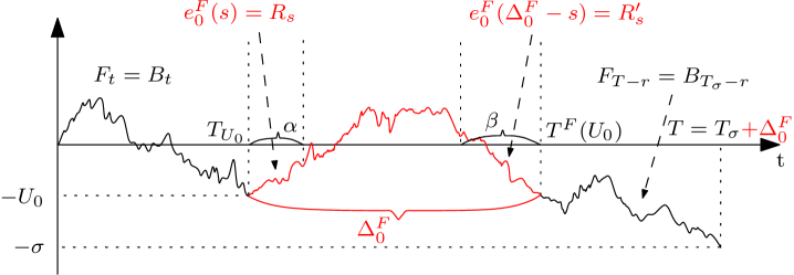
Figure 11: The coupling of contour functions stated as Proposition 6.23, with $s=s(t)=t-T_{U_{0}}$, $r=r(t)=T-t$.

Proposition 6.23.

For every $\varepsilon\in(0,1)$ and $\alpha,\beta>0$, there exists $T^{0}>0$ such that for every $T>T^{0}$, it is possible to couple $F,B,R,R^{\prime},U_{0}$ on the same probability space in such a way that with probability at least $1-\varepsilon$, one has $U_{0}=U_{1}^{F}$ and

$$F_{t}=B_{t},\,0\leq t\leq T^{F}(U_{0}-)=T_{U_{0}}\,,\qquad F_{T-t}=B_{T_{\sigma}-t},\,0\leq t\leq T-T^{F}(U_{0})=T_{\sigma}-T_{U_{0}}\,,$$

and

$$e^{F}_{0}(t)=R_{t},\quad 0\leq t\leq\alpha\,,\qquad e^{F}_{0}(\Delta_{0}^{F}-t)=R^{\prime}_{t},\quad 0\leq t\leq\beta\,,$$

and finally

$$\inf_{[\alpha,\infty)}R\wedge\inf_{[\beta,\infty)}R^{\prime}=\min_{[\alpha,\Delta^{F}_{0}-\beta]}e^{F}_{0}\,.$$

Proof.

By Lemma 6.22, for $T$ large enough, say $T>T^{1}$, it is possible to couple two sequences $\Delta_{1},\Delta_{2},\ldots$ and $\Delta^{\prime}_{0},\Delta^{\prime}_{1},\Delta^{\prime}_{2},\ldots$ on the same probability space such that

• $(\Delta_{1},\Delta_{2},\ldots)$ has the law of the jump sizes of $(T_{x},0\leq x\leq\sigma)$ ranked in size-biased order, and

• $(\Delta^{\prime}_{0},\Delta^{\prime}_{1},\Delta^{\prime}_{2},\ldots)$ has the law of $(\Delta_{1},\Delta_{2},\ldots)$ conditionally given $\sum_{i\geq 1}\Delta_{i}=T$,

in such a way that on an event $\mathcal{E}_{1}$ of probability at least $1-\varepsilon/2$, one has

$$\Delta_{i}=\Delta^{\prime}_{i}\,,\qquad i\geq 1\,,\qquad\mbox{ and }\qquad\Delta^{\prime}_{0}>T/2\,.$$

Extending the probability space if necessary, we can assume that it also supports an independent family of random variables $e_{0},e_{1},e_{2},\ldots$ that are independent normalized Brownian excursions, and $U_{0},U_{1},U_{2},\ldots$ that are independent uniform random variables in $[0,\sigma]$, independent of all the rest.

By Itô’s synthesis of Brownian motion from its excursions, if we set, for $i\geq 1$,

$$B_{t}=-U_{i}+\frac{e_{i}(\Delta_{i}(t-\sum_{j:U_{j}<U_{i}}\Delta_{j}))}{\sqrt{\Delta_{i}}}\,,$$

whenever $\sum_{j\geq 1:U_{j}<U_{i}}\Delta_{i}<t\leq\sum_{j\geq 1:U_{j}\leq U_{i}}\Delta_{j}$, then this a.s. extends to a continuous path $(B_{t},0\leq t\leq\sum_{i\geq 1}\Delta_{i})$ which is a trajectory of Brownian motion stopped when first hitting $-\sigma$, which occurs at time $T_{\sigma}=\sum_{i\geq 1}\Delta_{i}$. Similarly, setting, this time for $i\geq 0$,

$$F(t)=-U_{i}+\frac{e_{i}(\Delta_{i}^{\prime}(t-\sum_{j:U_{j}<U_{i}}\Delta^{\prime}_{j}))}{\sqrt{\Delta^{\prime}_{i}}}\,,$$

whenever $\sum_{j\geq 0:U_{j}<U_{i}}\Delta^{\prime}_{i}<t\leq\sum_{j\geq 0:U_{j}\leq U_{i}}\Delta^{\prime}_{j}$, this extends to a trajectory of a first-passage bridge $(F(t),0\leq t\leq T)$ from $0$ to $-\sigma$, as the notation suggests, and if we set $\Delta^{F}_{i}=\Delta^{\prime}_{i}$ for $i\geq 0$ then $(\Delta^{F}_{i},i\geq 0)$ is indeed a size-biased ordering of the jumps of the first hitting time process of negative values of $F$.

On the event $\mathcal{E}_{1}$, the two processes $B$ and $F$ coincide on the interval $[0,\sum_{j\geq 1:U_{j}<U_{0}}\Delta_{j}]$, and likewise, $B_{T_{\sigma}-\cdot}$ and $F(T-\cdot)$ coincide on $[0,\sum_{j\geq 1:U_{j}>U_{0}}\Delta_{j}]$. This yields the first displayed identity in the statement, since by construction

$$\sum_{j\geq 1:U_{j}<U_{0}}\Delta^{\prime}_{j}=T^{F}(U_{0}-)\,,\qquad\sum_{j\geq 1:U_{j}<U_{0}}\Delta_{j}=\sum_{j\geq 1:U_{j}\leq U_{0}}\Delta_{j}=T_{U_{0}}\,,$$

while we have

$$\sum_{j\geq 1:U_{j}>U_{0}}\Delta^{\prime}_{j}=T-T^{F}(U_{0})\,,\qquad\sum_{j\geq 1:U_{j}>U_{0}}\Delta_{j}=\sum_{j\geq 1:U_{j}\geq U_{0}}\Delta_{j}=T_{\sigma}-T_{U_{0}}\,.$$

Finally, in this construction, and still in restriction to $\mathcal{E}_{1}$, $e_{0}^{F}=e_{0}(\Delta_{0}^{\prime}\cdot)/\sqrt{\Delta_{0}^{\prime}}$ is an excursion of Brownian motion with duration $\Delta^{\prime}_{0}>T/2$. At this point, we can apply Proposition 3 in [19], in the same way as in the proof of Proposition 4 therein. Up to a further extension of the probability space, as soon as $T$ is chosen large enough, say $T>T^{2}$, we can couple this “long” excursion with two independent Bessel processes $R,R^{\prime}$ (and independent of all previously defined random variables) in such a way that the three last identities of the statement are satisfied on an event $\mathcal{E}_{2}$ with probability at least $1-\varepsilon/2$. This yields the wanted result with $T^{0}=T^{1}\vee T^{2}$, since the intersection $\mathcal{E}_{1}\cap\mathcal{E}_{2}$ has probability at least $1-\varepsilon$. ∎

6.6.2 Isometry of balls in $\textup{{BD}}_{T,\sigma}$ and $\textup{{IBD}}_{\sigma}$

We fix $\sigma\in(0,\infty)$, $\varepsilon>0$ and let $r\geq 0$. With the coupling from the preceding section at hand, the proof the proposition is a minor modification of [19, Proof of Proposition 4] (see also Proposition 6.4 and its proof). We will point at the necessary modifications and then leave it to reader to fill in the remaining details.

We work in the notation and with the processes of Proposition 6.23 and denote additionally by $\gamma=(\gamma_{u},0\leq u\leq\sigma)$ a standard Brownian bridge with duration $\sigma$, multiplied by $\sqrt{3}$.

Proof of Proposition 6.20.

Let us first introduce a few events. For $K>0$, put

$$\mathcal{E}^{1}(K)=\left\{\max_{[0,\sigma]}\gamma<K\right\}.$$

Then, given $A>0$, with $\zeta=(\zeta_{t},t\geq 0)$ denoting a Brownian motion started at $0$, let

$$\mathcal{E}^{2}(A,K)=\left\{\min_{[0,A]}\zeta<-10r-K,\,\min_{[A,A^{2}]}\zeta<-10r-K,\,\min_{[A^{2},A^{4}]}\zeta<-10r-K\right\},$$

and for $A>0$ and $\alpha>0$, set

$$\mathcal{E}^{3}(A,\alpha)=\left\{\inf_{[\alpha,\infty)}R\wedge\inf_{[\alpha,\infty)}R^{\prime}>A^{4}\right\}.$$

We first choose $K$ sufficiently large such that $\mathbb{P}(\mathcal{E}^{1})\geq 1-\varepsilon/6.$ Then, standard properties of Brownian motion allow us to find $A>0$ such that $\mathbb{P}(\mathcal{E}^{2})\geq 1-\varepsilon/6$ as well, and with such a fixed $A$, we find by transience of the Bessel process an $\alpha>0$ large enough such that $\mathbb{P}(\mathcal{E}^{3})>1-\varepsilon/3$.

Let us next recall the contour process $Y^{\sigma}$ of $\textup{{IBD}}_{\sigma}$ specified just before Definition 2.8 in terms of the Bessel processes $R$ and $R^{\prime}$ and the Brownian motion $B$ stopped at times $T_{U_{0}}$ and $T_{\sigma}$. We obtain that on the coupling event $\mathcal{E}^{4}=\mathcal{E}^{4}(\alpha,T)$ described in the statement of Proposition 6.23 (with $\beta=\alpha$), in the notation from there,

$$F_{t}=Y^{\sigma}_{t}\quad\mbox{for }t\in[0,T_{U_{0}}+\alpha]\,,\quad\mbox{ and }\quad F_{T-t}+\sigma=Y^{\sigma}_{-t}\quad\mbox{for }t\in[0,T_{\sigma}-T_{U_{0}}+\alpha]\,.$$

Concerning $\textup{{BD}}_{T,\sigma}$, we use the notation from Section 6.2.1 (note however that $\sigma$ is now a constant not depending on the volume $T$). We build the label process of $\textup{{BD}}_{T,\sigma}$ in the following way: Consider a Brownian bridge $\gamma$ as specified above, independent of $(F,B,R,R^{\prime},U_{0})$. Then let $Z=Z^{F-\underline{F}}$ be the random snake driven by $F-\underline{F}$, and set

$$W_{t}=\gamma_{-\underline{F}_{t}}+Z_{t},\quad 0\leq t\leq T.$$

Concerning $\textup{{IBD}}^{\sigma}$, we write $Z^{\textup{I}}=Z^{Y^{\sigma}-\underline{\underline{Y}}^{\sigma}}$ for the random snake driven by $Y^{\sigma}-\underline{\underline{Y}}^{\sigma}$, see Definition 2.8, and $W^{\textup{I}}_{t}=\gamma_{-\underline{\underline{Y}}^{\sigma}_{t}}+Z^{\textup{I}}$ for the label process associated with $\textup{{IBD}}_{\sigma}$. Of course, we choose to use the same bridge $\gamma$ to construct $W$ and $W^{\textup{I}}$.

We now work always conditionally on $(F,B,R,R^{\prime},U_{0})$. Similarly to the considerations around (6.14) and (6.15) in the proof of Proposition 6.4, one checks that on the event $\mathcal{E}^{4}$, the covariance function of

$$(W_{t},0\leq t\leq T_{U_{0}}+\alpha),(W_{T-t},0\leq t\leq T_{\sigma}-T_{U_{0}}+\alpha)$$

on the one hand, and

$$(W^{\textup{I}}_{t},0\leq t\leq T_{U_{0}}+\alpha),(W^{\textup{I}}_{-t},0\leq t\leq T_{\sigma}-T_{U_{0}}+\alpha)$$

on the other hand, are the same. Consequently, we may assume that $W$ and $W^{\textup{I}}$ are coupled in such a way that, on the event $\mathcal{E}^{4}$,

$$W_{t}=W^{\textup{I}}_{t}\quad\hbox{ for all }t\in[0,T_{U_{0}}+\alpha],\quad W_{T-t}=W^{\textup{I}}_{-t}\quad\hbox{ for all }t\in[0,T_{\sigma}-T_{U_{0}}+\alpha].$$

From Proposition 6.23, we derive that for the choice of $\alpha$ from above, the coupling event $\mathcal{E}^{4}(\alpha,T)$ has probability at least $1-\varepsilon/3$ provided $T$ is sufficiently large, and we shall work with such a $T$. The reminder of the proof is now close to [19, Proof of Proposition 4]. For every $x\geq 0$, let

$$\eta_{\textup{l}}(x) =\sup\{0\leq t\leq\Delta_{0}^{F}/2:e_{0}^{F}(t)=x\}+T_{U_{0}},$$

$$\eta_{\textup{r}}(x) =\Delta_{0}^{F}-\inf\{\Delta_{0}^{F}/2\leq t\leq\Delta_{0}^{F}:e_{0}^{F}(t)=x\}+T_{\sigma}-T_{U_{0}},$$

and

$$\eta_{\textup{l}}^{\textup{I}}(x) =\sup\{t\geq 0:R_{t}=x\}+T_{U_{0}},$$

$$\eta_{\textup{r}}^{\textup{I}}(x) =\sup\{t\geq 0:R_{t}^{\prime}=x\}+T_{\sigma}-T_{U_{0}}.$$ (6.41)

Then the process $(Z^{\textup{I}}_{\eta_{\textup{l}}^{\textup{I}}(x)},x\geq 0)$ has the law of a standard Brownian motion started at $Z^{\textup{I}}_{T_{U_{0}}}=0$. Choosing this Brownian motion in the definition of the event $\mathcal{E}^{2}$ from above, so that on $\mathcal{E}^{2}$, we have

$$\min_{x\in[0,A]}Z^{\textup{I}}_{\eta_{\textup{l}}^{\textup{I}}(x)}<-6r-K,\,\min_{x\in[A,A^{2}]}Z^{\textup{I}}_{\eta_{\textup{l}}^{\textup{I}}(x)}<-6r-K,\,\min_{x\in[A^{2},A^{4}]}Z^{\textup{I}}_{\eta_{\textup{l}}^{\textup{I}}(x)}<-6r-K,$$ (6.42)

we shall from now on work on the intersection of events

$$\mathcal{F}=\mathcal{E}^{1}\cap\mathcal{E}^{2}\cap\mathcal{E}^{3}\cap\mathcal{E}^{4},$$ (6.43)

which has probability at least $1-\varepsilon$.

On $\mathcal{E}^{3}\cap\mathcal{E}^{4}$, we note that $\min_{[\alpha,\Delta_{0}^{F}-\alpha]}e^{F}_{0}=\inf_{[\alpha,\infty)}R\wedge\inf_{[\alpha,\infty)}R^{\prime}>A^{4}$, whence for $x\in[0,A^{4}]$, $\eta_{\textup{l}}(x)=\eta_{\textup{l}}^{\textup{I}}(x)<T_{U_{0}}+\alpha$ and $\eta_{\textup{r}}(x)=\eta_{\textup{r}}^{\textup{I}}(x)<T_{\sigma}-T_{U_{0}}+\alpha$. It follows that for any $x\in[0,A^{4}]$,

$$Z_{\eta_{\textup{l}}(x)}=Z_{\eta_{\textup{l}}^{\textup{I}}(x)}^{\textup{I}}=Z_{-\eta_{\textup{r}}^{\textup{I}}(x)}^{\textup{I}}=Z_{T-\eta_{\textup{r}}(x)}.$$

We are now almost in a setting where we can appeal to the reasoning in [19, Section 3.2]. We should still adapt the definition of $\tilde{d}_{W}(s,t)$ given just before Lemma 6.8 to the setting considered here. Let $s,t\in[0,T]$. If $s,t$ lie both in either $[0,T_{U_{0}}+\Delta_{0}^{F}/2]$ or in $[T_{U_{0}}+\Delta_{0}^{F}/2,T]$, we let

$$d^{\prime}_{W}(s,t)=W_{s}+W_{t}-2\min_{[s\wedge t,s\vee t]}W.$$

Otherwise, we set

$$d^{\prime}_{W}(s,t)=W_{s}+W_{t}-2\min_{[0,s\wedge t]\cup[s\vee t,T]}W.$$

Recall the definition of the pseudo-metric $D(s,t)$ associated to the Brownian disk $\textup{{BD}}_{T,\sigma}$. The following statement replaces Lemma 6.8 and is close to [19, Lemma 5(i)].

Lemma 6.24.

Assume $\mathcal{F}$ holds.

1. For every $t\in[\eta_{\textup{l}}(A),T-\eta_{\textup{r}}(A)]$, $D(0,t)>r$.

2. For every $s,t\in[0,\eta_{\textup{l}}(A)]\cup[0,T-\eta_{\textup{r}}(A)]$ with $\max\{D(0,s),D(0,t)\}\leq r$, it holds that

   $$D(s,t)=\inf_{s_{1},t_{1},\dots,s_{k},t_{k}}\sum_{i=1}^{k}d^{\prime}_{W}(s_{i},t_{i}),$$

   where the infimum is over all possible choices of $k\in\mathbb{N}$ and reals $s_{1},\dots,s_{k},t_{1},\dots,t_{k}\in[0,\eta_{\textup{l}}(A^{2})]\cup[T-\eta_{\textup{r}}(A^{2}),T]$ such that $s_{1}=s,t_{k}=t$, and $d_{F}(t_{i},s_{i+1})=0$ for $1\leq i\leq k-1$.

Proof.

One can follow the same line of reasoning as in [19, Proof of Lemma 5(i)], with one small modification, which is apparent from the proof of (a), so let us prove this part. If $t\in[\eta_{\textup{l}}(A),T-\eta_{\textup{r}}(A)]$, then by the cactus bound (6.17),

$$D(0,t)\geq W_{t}-2\max\left\{\min_{[0,t]}W,\min_{[t,T]}W\right\}\geq-\max\left\{\min_{[0,\eta_{\textup{l}}(A)]}W,\min_{[T-\eta_{\textup{r}}(A),T]}W\right\}.$$

Recalling that $W_{t}=\gamma_{-\underline{F}_{t}}+Z_{t}$, we first remark that on the event $\mathcal{E}^{3}\cap\mathcal{E}^{4}$, since $\eta_{\textup{l}}(A)<T_{U_{0}}+\alpha$, we have $Z=Z^{\textup{I}}$ on $[0,\eta_{\textup{l}}(A)]$. Since $\eta_{\textup{l}}([0,A])\subset[0,\eta_{\textup{l}}(A)]$, it follows now from (6.42) that the minimum of $Z$ on $[0,\eta_{\textup{l}}(A)]$ is bounded from above by $-6r-K$. But on $\mathcal{E}^{1}$, $\max\gamma<K$, so that $\min_{[0,\eta_{\textup{l}}(A)]}W\leq-6r$. A similar argument holds for the second minimum, so that in fact $D(0,t)\geq 6r$ whenever $t\in[\eta_{\textup{l}}(A),T-\eta_{\textup{r}}(A)]$. For (b), one can follow [19, Proof of Lemma 5(i)], or modify the proof of (b) in Lemma 6.8. ∎

Entirely similar, one finds the corresponding statement for the pseudo-metric $D^{\textup{I}}$ of $\textup{{IBD}}_{\sigma}$ that replaces Lemma 6.9: In the statement there, $\eta_{\textup{r}}$ and $\eta_{\textup{l}}$ have to be replaced by $\eta_{\textup{r}}^{\textup{I}}$ and $\eta_{\textup{l}}^{\textup{I}}$ as defined under (6.6.2), and $D_{\theta}$, $d_{W^{\theta}}$ by $D^{\textup{I}}$ and $d_{W^{\textup{I}}}$. Following again [19], or adapting the second part of the proof of Proposition 6.4, these two lemmas lead to the stated isometry between $B_{r}(\textup{{BD}}_{T,\sigma})$ and $B_{r}(\textup{{IBD}}_{\sigma})$ on the event $\mathcal{F}$ of probability at least $1-\varepsilon$, finishing thereby the proof of Proposition 6.20. ∎

It remains to show how Proposition 6.20 can be improved to the coupling stated in Theorem 3.12.

6.6.3 Proof of Theorem 3.12

The proof is close in spirit to that of Theorem 3.7: for a fixed $r>0$, we must find some $r_{0}>r$ large enough so that for all $T$ sufficiently large, the ball $B_{r_{0}}(\textup{{BD}}_{T,\sigma})$ contains with high probability an open set $A_{\textup{{BD}}}$ that is homeomorphic to the pointed closed disk $\overline{\mathbb{D}}\setminus\{0\}$ and that, in turn, contains the ball $B_{r}(\textup{{BD}}_{T,\sigma})$ with high probability. Then we will apply the coupling Proposition 6.20 in order to couple the balls $B_{r_{0}}(\textup{{BD}}_{T,\sigma})$ and $B_{r_{0}}(\textup{{IBD}}_{\sigma})$. The set $A_{\textup{{BD}}}$ will be defined as a region bounded by certain geodesic paths.

We use a similar notation to that of the proof of Theorem 3.7, setting $\textup{{Y}}=([0,T]/\{D=0\},D,\rho)$ and letting $p_{\textup{{Y}}}$ be the associated canonical projection, so that $Y$ has the law of the Brownian disk $\textup{{BD}}_{T,\sigma}$ with root $\rho=p_{\textup{{Y}}}(0)$. We will also use the geodesic paths $\Gamma_{s},s\in[0,T]$, in Y respectively from $p_{\textup{{Y}}}(s)$ to $x_{*}=p_{\textup{{Y}}}(s_{*})$ defined around Lemma 6.15, together with the properties stated there.

Let $a_{0}>0$ be a large number to be specified later on. We let $A_{\textup{{BD}}}^{0}=[0,\eta_{\textup{l}}(a_{0})]\cup[T-\eta_{\textup{r}}(a_{0}),T]$, where $\eta_{\textup{l}},\eta_{\textup{r}}$ are defined in the proof of Proposition 6.20. We will work on the event that $s_{*}\notin A_{\textup{{BD}}}^{0}$, a fact that will be granted later with high probability by the fact that $T$ is going to infinity. With our notation, the definition of $A_{\textup{{BD}}}^{0}$ is the exact same as $O_{\textup{{BD}}}^{0}$ in the proof of Theorem 3.7, but note that by contrast, the points $p_{\textup{{Y}}}(\eta_{\textup{l}}(a_{0}))$ and $p_{\textup{{Y}}}(T-\eta_{\textup{r}}(a_{0}))$ are now equal, and we denote it by $x_{0}$. Note in passing that $x_{0}\notin\partial\textup{{Y}}$ by Lemma 6.12. We let $t_{*}\in A^{0}_{\textup{{BD}}}$ be such that $W_{t_{*}}=\min_{A^{0}_{\textup{{BD}}}}W$. The geodesic paths $\Gamma_{\eta_{l}(a_{0})}$ and $\Gamma_{T-\eta_{r}(a_{0})}$ both start from $x_{0}$, but by (d) in Lemma 6.15, they become disjoint until they meet again for the first time at the point $p_{\textup{{Y}}}(t_{*})$. Therefore, the segments of these geodesics between $x_{0}$ and $p_{\textup{{Y}}}(t_{*})$ form a simple loop $P$, which is disjoint from the boundary $\partial\textup{{Y}}$ by (c) in Lemma 6.12. We point at Figure 12 for an illustration. The analog of Lemma 6.16 is the following.

Lemma 6.25.

The set $P$ is a simple loop in Y containing $x_{0}$, and that does not intersect $\partial\textup{{Y}}$. Letting $A_{\textup{{BD}}}$ be the connected component of $\textup{{Y}}\setminus P$ that contains $p_{\textup{{Y}}}(0)$, then $A_{\textup{{BD}}}$ is almost surely homeomorphic to the pointed closed disk $\overline{\mathbb{D}}\setminus\{0\}$, and is the interior of the set $p_{\textup{{Y}}}(A^{0}_{\textup{{BD}}})$ in Y.

Proof.

The proof is very similar to that of Lemma 6.16. The fact that $A_{\textup{{BD}}}$ is a.s. homeomorphic to $\overline{\mathbb{D}}\setminus\{0\}$ is a direct consequence of the fact that Y is homeomorphic to $\overline{\mathbb{D}}$ and that $P$ is a simple loop not intersecting $\partial\textup{{Y}}$. The only thing that remains to be proved given our discussion so far is that $A_{\textup{{BD}}}$ is indeed the interior of $p_{\textup{{Y}}}(A^{0}_{\textup{{BD}}})$. However, using the exact same definition of the paths $\Xi_{s}$, it is simple to see that a point in $p_{\textup{{Y}}}(A^{0}_{\textup{{BD}}})$ is linked to $\partial\textup{{Y}}$, and hence to $p_{\textup{{Y}}}(0)$, by a simple path that intersects $P$, if at all, only at its starting point. It remains to verify that for every $x\in\textup{{Y}}\setminus p_{\textup{{Y}}}(A^{0}_{\textup{{BD}}})$, we can find a simple path from $x$ to $p_{\textup{{Y}}}(s_{*})$ that possibly intersects $P$ only at its origin. Writing $x=p_{\textup{{Y}}}(s)$, we leave it to the reader that such a path can be obtained by concatenating segments of the paths $p_{\textup{{Y}}}\circ\Xi_{s}$ and $p_{\textup{{Y}}}\circ\Xi_{s_{*}}$. The conclusion follows. ∎

Now for a fixed $r>0$ and $\varepsilon>0$, we choose $a_{0}>0$ large enough so that

$$\mathbb{P}\left(\min_{[0,a_{0}]}Z^{\textup{I}}_{\eta^{\textup{I}}_{\textup{l}}(\cdot)}<-2r\right)\geq 1-\varepsilon/4,$$

and then let $r_{0}>r$ be large enough so that

$$\mathbb{P}\left(\omega(W^{\textup{I}},[-\eta_{r}^{\textup{I}}(a_{0}),\eta_{l}^{\textup{I}}(a_{0})])\leq r_{0}/2\right)\geq 1-\varepsilon/4\,.$$

We use this value of $r_{0}$ to apply the coupling of $\textup{{Y}}=\textup{{BD}}_{T,\sigma}$ and $\textup{{IBD}}_{\sigma}$ of Proposition 6.20, guaranteeing that the balls of radius $r_{0}$ in these pointed spaces are isometric with probability at least $1-\varepsilon/2$. From there, we conclude exactly as in the end of the proof of Theorem 3.7, replacing $O_{\textup{{BD}}}$ and $O_{\textup{{BHP}}}=I(O_{\textup{{BD}}})$ by $A_{\textup{{BD}}}$ and $A_{\textup{{BHP}}}=I(A_{\textup{{BD}}})$, where $I$ is defined as before Corollary 6.10 and defines an isometry between $B_{r_{0}}(\textup{{Y}})$ and $B_{r_{0}}(\textup{{IBD}}_{\sigma})$ on the coupling event $\mathcal{F}$ given by (6.43) (note that on this event, one has in particular $\eta_{\textup{l}}(x)=\eta^{\textup{I}}_{\textup{l}}(x)$ and $\eta_{\textup{r}}(x)=\eta_{\textup{r}}^{\textup{I}}(x)$ for every $x\leq A^{4}$, and without loss of generality, we can choose $A$ so that $A^{4}>a_{0}$.) This completes the proof of Theorem 3.12.

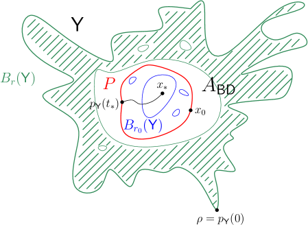
Figure 12: Illustration of the proof of Theorem 3.12. Note that in this figure, we look at the disk $\textup{{Y}}=\textup{{BD}}_{T,\sigma}$ from above. The ball $B_{r}(\textup{{Y}})$ contains the full boundary of Y and is included in the larger ball $B_{r_{0}}(\textup{{Y}})$, whose boundary in Y is indicated by the loops in blue. The ball $B_{r_{0}}(\textup{{Y}})$ encompasses the open set $A_{\textup{{BD}}}$, which is homeomorphic to the pointed disk $\overline{\mathbb{D}}\setminus\{0\}$. The set $A_{\textup{{BD}}}$ is bordered by the boundary of Y and the simple loop $P$ (in red) in Y. The loop $P$ is formed by two segments of geodesics between $x_{0}$ and $p_{\textup{{Y}}}(t_{\ast})$.

6.7 Infinite-volume Brownian disk (Theorem 3.2)

For proving Theorem 3.2, we will combine the convergence towards the Brownian disk $\textup{{BD}}_{T,\sigma}$ proved in [9, Theorem 1] (see Display (6.27)) with the couplings Theorem 3.12 and Proposition 3.14. We work in the usual setting specified in Section 4.5.4.

Proof of Theorem 3.2.

Assume $1\ll\sigma_{n}\ll\sqrt{n}$ and $a_{n}\sim(4/9)^{1/4}\sqrt{\sigma_{n}/\sigma}$ for some $\sigma\in(0,\infty)$. We have to show that for each $r\geq 0$,

$$B_{r}\left(a_{n}^{-1}\cdot Q_{n}^{\sigma_{n}}\right)\xrightarrow[n\to\infty]{(d)}B_{r}(\textup{{IBD}}_{\sigma})$$

in distribution in $\mathbb{K}$. We fix $\varepsilon>0$ and $r\geq 0$. By Theorem 3.12, we find $T_{0}$ such that for all $T\geq T_{0}$, we can construct on the same probability space copies of $\textup{{BD}}_{T,\sigma}$ and $\textup{{IBD}}_{\sigma}$ such that with probability at least $1-\varepsilon$, we have an isometry of balls

$$B_{r}(\textup{{BD}}_{T,\sigma})=B_{r}(\textup{{IBD}}_{\sigma}).$$ (6.44)

By Proposition 3.14, we find $R_{0}\geq T_{0}/(2\sigma^{2})$ such that for $R\geq R_{0}$ and $n$ sufficiently large, we can construct on the same probability space copies of $Q_{n}^{\sigma_{n}}$ and $Q_{R\sigma_{n}^{2}}^{\sigma_{n}}$ such that with probability at least $1-\varepsilon$, there is the isometry

$$B_{ra_{n}}(Q_{n}^{\sigma_{n}})=B_{ra_{n}}\left(Q_{R\sigma_{n}^{2}}^{\sigma_{n}}\right).$$ (6.45)

Now let $F:\mathbb{K}\rightarrow\mathbb{R}$ be a bounded and continuous function and $R\geq R_{0}$. We assume that $Q_{n}^{\sigma_{n}}$ and $Q_{R\sigma_{n}^{2}}^{\sigma_{n}}$ are constructed on the same probability space such that (6.45) holds, and similarly $\textup{{BD}}_{2R\sigma^{2},\sigma}$ and $\textup{{IBD}}_{\sigma}$ so that (6.44) is satisfied. We write

$$\left|\mathbb{E}\left[F\left(B_{r}\left(a_{n}^{-1}\cdot Q_{n}^{\sigma_{n}}\right)\right)\right]-\mathbb{E}\left[F\left(B_{r}\left(\textup{{IBD}}_{\sigma}\right)\right)\right]\right|$$

$$\quad\quad\leq\left|\mathbb{E}\left[F\left(a_{n}^{-1}\cdot B_{ra_{n}}\left(Q_{n}^{\sigma_{n}}\right)\right)-F\left(a_{n}^{-1}\cdot B_{ra_{n}}\left(Q_{R\sigma_{n}^{2}}^{\sigma_{n}}\right)\right)\right]\right|$$

$$\quad\quad\quad+\left|\mathbb{E}\left[F\left(a_{n}^{-1}\cdot B_{ra_{n}}\left(Q_{R\sigma_{n}^{2}}^{\sigma_{n}}\right)\right)\right]-\mathbb{E}\left[F\left(B_{r}\left(\textup{{BD}}_{2\sigma^{2}R,\sigma}\right)\right)\right]\right|$$

$$\quad\quad\quad+\left|\mathbb{E}\left[F\left(B_{r}(\textup{{BD}}_{2\sigma^{2}R,\sigma})\right)-F\left(B_{r}\left(\textup{{IBD}}_{\sigma}\right)\right)\right]\right|.$$

Using (6.45) and (6.44) (note that $2\sigma^{2}R\geq T_{0}$), the first and third summand on the right hand side are bounded from above by $2\varepsilon\sup F$. The scaling property $\lambda\cdot\textup{{BD}}_{1,\sigma}=_{d}\textup{{BD}}_{\lambda^{4},\lambda^{2}\sigma}$ for $\lambda>0$ combined with the convergence (6.27) implies that the second summand converges to zero as $n\rightarrow\infty$. This finishes the proof of Theorem 3.2. ∎

6.8 Brownian disk limits (Corollaries 3.15, 3.16, 3.17 and 3.18).

Proof of Corollaries 3.15, 3.16, 3.17 and 3.18..

We have to show that for each $r\geq 0$, when $T$ tends to infinity, $B_{r}(\textup{{BD}}_{T,\sigma(T)})$ converges in law to the ball of radius $r$ around the root in the limit space $\mathcal{X}$ that appears in the corresponding corollary. As usual, we consider only the case $r=1$.

Let $F:\mathbb{K}\rightarrow\mathbb{R}$ be bounded and continuous. For $T\in\mathbb{N}$ and $n\in\mathbb{N}$, we set

$$m_{n}(T)=Tn,\quad\sigma_{n}(T)=\lfloor\sigma(T)\sqrt{2n}\rfloor,\quad a_{n}=(8/9)^{1/4}n^{1/4}.$$

We write

$$\left|\mathbb{E}\left[F\left(B_{1}\left(\textup{{BD}}_{T,\sigma(T)}\right)\right)\right]-\mathbb{E}\left[F\left(B_{1}\left(\mathcal{X}\right)\right)\right]\right|$$

$$\quad\quad\leq\left|\mathbb{E}\left[F\left(B_{1}\left(\textup{{BD}}_{T,\sigma(T)}\right)\right)\right]-\mathbb{E}\left[F\left(a_{n}^{-1}\cdot B_{a_{n}}\left(Q_{m_{n}(T)}^{\sigma_{n}(T)}\right)\right)\right)\right|$$

$$\quad\quad\quad+\left|\mathbb{E}\left[F\left(a_{n}^{-1}\cdot B_{a_{n}}\left(Q_{m_{n}(T)}^{\sigma_{n}(T)}\right)\right)\right]-\mathbb{E}\left[F\left(B_{1}\left(\mathcal{X}\right)\right)\right]\right|.$$

For each fixed $T\in\mathbb{N}$, the convergence [9, Theorem 1] towards the Brownian disk with volume $T$ and perimeter $\sigma(T)$ (see (6.27) above) implies that the first summand on the right hand side is bounded by $\varepsilon$, provided $n\geq n_{0}(T)$.

Concerning the second summand, we argue by contradiction that for large enough $T$, there exists $n_{0}=n_{0}=(T,\varepsilon)$ such that for any $n\geq n_{0}$, the second summand is bounded by $\varepsilon$ as well. Indeed, assuming this is not the case, we find a sequence of integers $(T_{k},k\in\mathbb{N})$ with $T_{k}\rightarrow\infty$ and a sequence of integers $(n_{k},k\in\mathbb{N})$ with $n_{k}$ depending on $T_{k}$ and $n_{k}\rightarrow\infty$, such that

$$\left|\mathbb{E}\left[F\left(a_{n_{k}}^{-1}\cdot B_{a_{n_{k}}}\left(Q_{m_{n_{k}}(T_{k})}^{\sigma_{n_{k}}(T_{k})}\right)\right)\right]-\mathbb{E}\left[F\left(B_{1}\left(\mathcal{X}\right)\right)\right]\right|>\varepsilon.$$ (6.46)

We put $T_{0}=n_{0}=0$ and for $n\in\mathbb{N}$,

$$\tilde{a}_{n}=(8/9)^{1/4}\left(n/T_{k}\right)^{1/4},\quad\tilde{\sigma}_{n}=\lfloor\sigma(T_{k})\sqrt{2n/T_{k}}\rfloor,\quad\textup{ if }T_{k}n_{k-1}<n\leq T_{k}n_{k}.$$

For concreteness, we now consider the framework of Corollary 3.15, where $\mathcal{X}=\textup{{BP}}$ and $\sigma(T)\rightarrow 0$ as $T$ tends to infinity. Then $\tilde{\sigma}_{n}\ll\sqrt{n}$, and $\sqrt{\tilde{\sigma}_{n}}\ll\tilde{a}_{n}\ll n^{1/4}$, so that we can apply the convergence towards BP proved in Theorem 3.1 (with $\sigma_{n}$ and $a_{n}$ there replaced by $\tilde{\sigma}_{n}$ and $\tilde{a}_{n}$). However, observing the quadrangulations at sizes $m_{k}=T_{k}n_{k}$, (6.46) contradicts the convergence towards BP.

In the setting of Corollary 3.16, we use Theorem 3.2 instead of Theorem 3.1 and the fact that $\sigma(T)\rightarrow\varsigma\in(0,\infty)$ as $T\rightarrow\infty$. An identical argument allows us to finish the proof in this case, with $\mathcal{X}$ given by $\textup{{IBD}}_{\varsigma}$. In the framework of Corollary 3.18 where $\sigma(T)/T\rightarrow\infty$ as $T$ tends to infinity, we apply Theorem 3.5 instead.

Let us finally look at Corollary 3.17. There, $\sigma(T)\rightarrow\infty$ and $\sigma(T)/T\rightarrow\theta\in[0,\infty)$. If $\theta=0$, then, along sequences $(T_{m},m\in\mathbb{N})$ tending to infinity for which $\sigma(T_{m})/\sqrt{T_{m}}\rightarrow 0$ as $m\rightarrow\infty$, we follow the same argumentation by contradiction and use Theorem 3.3, whereas if $\liminf_{m\rightarrow\infty}\sigma(T_{m})/\sqrt{T_{m}}>0$, the corollary is a direct consequence of Theorem 3.7, and so is it in the case $\theta>0$. ∎

6.9 Infinite continuum random tree (Theorem 3.5)

We use the second construction of $\textup{{ICRT}}=(\mathcal{T}_{Y},d_{Y},[0])$ from Section 2 in terms of a standard two-sided Brownian motion $(Y_{t},t\in\mathbb{R})$ with $Y_{0}=0$. Recall that Theorem 3.5 treats the regime $\sigma_{n}\gg\sqrt{n}$, and we explicitly allow $\sigma_{n}$ to grow faster than $n$.

Idea of the proof. Let $(\textup{$\mathfrak{f}$}_{n},\textup{$\mathfrak{l}$}_{n})$ be a random uniform element of $\textup{$\mathfrak{F}$}_{\sigma_{n}}^{n}$. We show that under the rescaling by a factor $\max\{1,\sqrt{n/\sigma_{n}}\}\ll a_{n}\ll\sqrt{\sigma_{n}}$, the labels of the first and last $ca_{n}^{2}$ trees of $\textup{$\mathfrak{f}$}_{n}$ converge to zero. For the rescaled submap $a_{n}^{-1}B_{ra_{n}}(Q_{n}^{\sigma_{n}})$, this means that for large $n$, the boundary dominates and folds the map into a tree-shaped object, which we identify with the ICRT in the limit $n\rightarrow\infty$.

Proof of Theorem 3.5.

We work in the usual setting, cf. 4.5.4. We will construct a set $\mathcal{R}_{n}$ which shares the properties of Lemma 5.7, and for that reason, we shall consider both $V(Q_{n}^{\sigma_{n}})$ and the corresponding length space ${\mathbf{Q}}_{n}^{\sigma_{n}}$, cf. Section 2.4.2.

Let $r\geq 0$. Still the vertex set $V(\textup{$\mathfrak{f}$}_{n})$ is naturally identified with points of ${\mathbf{Q}}_{n}^{\sigma_{n}}$, and we may consider the ball $B_{r}^{(0)}({\mathbf{Q}}_{n}^{\sigma_{n}})$ in ${\mathbf{Q}}_{n}^{\sigma_{n}}$ of radius $r$ around $\textup{$\mathfrak{f}$}_{n}(0)=(0)$ (with respect to the shortest-path metric $d$). Since the Gromov-Hausdorff distance between $B_{r}^{(0)}(Q_{n}^{\sigma_{n}})$ and $B_{r}^{(0)}({\mathbf{Q}}_{n}^{\sigma_{n}})$ is bounded by one, the theorem follows from Lemma 5.6 if we show that

$$B_{r}^{(0)}\left(a_{n}^{-1}\cdot{\mathbf{Q}}_{n}^{\sigma_{n}}\right)\xrightarrow[n\to\infty]{(d)}B_{r}(\mathcal{T}_{Y}),$$

for any scaling sequence $a_{n}$ with $\max\{1,\sqrt{n/\sigma_{n}}\}\ll a_{n}\ll\sqrt{\sigma_{n}}$.

For ease of reading, we restrict ourselves to the case $r=1$. Define

$$Y_{n}(t)=\left\{\begin{array}[]{l@{\quad\mbox{if }}l}\textup{{b}}_{n}(\sigma_{n}-1+(a_{n}^{2}/2)t)&-(\sigma_{n}-2)/a_{n}^{2}\leq t<0\\ \textup{{b}}_{n}((a_{n}^{2}/2)t)&0\leq t\leq\sigma_{n}/a_{n}^{2}\end{array}\right..$$

We extend the definition of $Y_{n}$ to all reals by letting $Y_{n}\equiv\textup{{b}}_{n}(\sigma_{n}/2)$ on $\{|t|>\sigma_{n}/a_{n}^{2}\}$. Note that $Y_{n}$ is càdlàg, with only one possible jump at $t=0$ of height $-\textup{{b}}_{n}(\sigma_{n}-1)$, which is stochastically bounded in probability as $n\rightarrow\infty$.

From Lemma 5.4 we know that $(1/\sqrt{2\sigma_{n}})(\textup{{b}}_{n}(\sigma_{n}t),0\leq t\leq 1)$ converges to a standard Brownian bridge $\mathbbm{b}$ in $\mathcal{C}([0,1],\mathbbm{R})$ as $n\rightarrow\infty$. From this and the fact that $a_{n}\ll\sqrt{\sigma_{n}}$, we obtain by standard reasoning (see, e.g., the proof of [5, Lemma 10])

$$\left(\frac{Y_{n}(t)}{a_{n}},t\in\mathbb{R}\right)\xrightarrow[n\to\infty]{(d)}\left(Y_{t},t\in\mathbb{R}\right),$$ (6.47)

where $Y=(Y_{t},t\in\mathbb{R})$ is a two-sided Brownian motion with $Y_{0}=0$, and the convergence holds in the space of càdlàg functions on $\mathbb{R}$ equipped with the compact-open topology.

By the Skorokhod representation theorem, we may assume that (6.47) holds almost surely uniformly over compacts. Let $\varepsilon>0$. By standard properties of Brownian motion, we find $\alpha>0$ and $n_{0}\in\mathbb{N}$ such that

$$\max\left\{\min_{[0,\alpha]}Y_{,}\min_{[-\alpha,0]}Y\right\}<-1\quad\textup{and}\quad\max\left\{\min_{[0,\alpha]}Y_{n},\min_{[-\alpha,0]}Y_{n}\right\}<-a_{n}$$ (6.48)

with probability at least $1-\varepsilon$ for $n\geq n_{0}$. We fix such an $\alpha$ and work on the event where (6.48) holds true. In the following, we make no difference between the root vertices $(0),\ldots,(\sigma_{n}-1)$ and the integers $0,\ldots,\sigma_{n}-1$. Moreover, recall that if $v$ is a vertex of a tree of $\textup{$\mathfrak{f}$}_{n}$, $\textup{$\mathfrak{r}$}(v)$ denotes the root vertex of that tree. For $v\in V(\textup{$\mathfrak{f}$}_{n})$, the cactus bound (4.4) gives

$$d_{\textup{gr}}((0),v)\geq-\max\left\{\min_{[0,\textup{$\mathfrak{r}$}(v)]}\textup{{b}}_{n},\min_{[\textup{$\mathfrak{r}$}(v),\sigma_{n}-1]}\textup{{b}}_{n}\right\}.$$ (6.49)

Every point $v$ in the length space ${\mathbf{Q}}_{n}^{\sigma_{n}}$ lies on a segment $e$ of length one connecting two vertices in $V(Q_{n}^{\sigma_{n}})$. We associate to each $v\in{\mathbf{Q}}_{n}^{\sigma_{n}}$ that endpoint $v^{\prime}\in V(Q_{n}^{\sigma_{n}})$ of $e$ which satisfies $d(0,v)\geq d_{\textup{gr}}(0,v^{\prime})$. We then extend the definition of $\mathfrak{r}$ to all points $v$ in ${\mathbf{Q}}_{n}^{\sigma_{n}}$ by letting $\textup{$\mathfrak{r}$}(v)=\textup{$\mathfrak{r}$}(v^{\prime})$, where we agree that $\textup{$\mathfrak{r}$}(v^{\bullet})=\infty$. Next define the subset of vertices

$$A_{n}=\left\{v\in{\mathbf{Q}}_{n}^{\sigma_{n}}:\textup{$\mathfrak{r}$}(v)\in[0,\alpha a_{n}^{2}/2]\cup[\sigma_{n}-1-\alpha a_{n}^{2}/2,\sigma_{n}-1]\right\}.$$

On the event where (6.48) holds, we have for vertices $v\in{\mathbf{Q}}_{n}^{\sigma_{n}}\setminus A_{n}$ by (6.49) (and by (4.1) for $v$ with $v^{\prime}=v^{\bullet}$) for $n$ sufficiently large

$$d(0,v)\geq d_{\textup{gr}}(0,v^{\prime})>a_{n}.$$

In words, $A_{n}$ contains the ball of radius $a_{n}$ around $(0)$ in $({\mathbf{Q}}_{n}^{\sigma_{n}},d)$.

We now consider the ICRT $(\mathcal{T}_{Y},d_{Y},[0])$ defined in terms of $Y$ and write $p_{Y}:\mathbb{R}\rightarrow\mathcal{T}_{Y}$ for the canonical projection. Define a subset $\mathcal{R}_{n}\subset{\mathbf{Q}}_{n}^{\sigma_{n}}\times\mathcal{T}_{Y}$ by putting

$$\mathcal{R}_{n}=\left\{(v,p_{Y}(t)):\begin{split}&v\in A_{n},t\in[0,\alpha]\hbox{ with }\textup{$\mathfrak{r}$}(v)=\lfloor(a_{n}^{2}/2)t\rfloor,\hbox{ or }\\ &v\in A_{n},t\in[-\alpha,0]\hbox{ with }\textup{$\mathfrak{r}$}(v)=\lfloor\sigma_{n}-1-(a_{n}^{2}/2)t\rfloor\end{split}\right\}.$$

On the event where (6.48) is true, the set $\mathcal{R}_{n}$ fulfills the conditions of Lemma 5.7 (with $\rho=(0)$, $\rho^{\prime}=p_{Y}(0)$, $r=a_{n}$). Thus it remains to show that $\lim_{n\rightarrow\infty}a_{n}^{-1}\textup{dis}(\mathcal{R}_{n})=0$ in probability. Note that in the notation from above, we have $|d(v,w)-d_{\textup{gr}}(v^{\prime},w^{\prime})|\leq 2$. Recall that the label function $\textup{$\mathfrak{L}$}_{n}$ is given by the labels $\textup{$\mathfrak{l}$}_{n}$ of the tree vertices, shifted according to the label of the corresponding root vertex which is carried by the bridge $\textup{{b}}_{n}$. By the distance bounds (4.3) and (4.5), we obtain for $v,w\in A_{n}$ with $\textup{$\mathfrak{r}$}(v)\leq\textup{$\mathfrak{r}$}(w)$,

$$\begin{split}\left|d(v,w)-\left(\textup{{b}}_{n}(\textup{$\mathfrak{r}$}(v))+\textup{{b}}_{n}(\textup{$\mathfrak{r}$}(w))-2\max\left\{\min_{[\textup{$\mathfrak{r}$}(v),\textup{$\mathfrak{r}$}(w)]}\textup{{b}}_{n},\min_{[0,\textup{$\mathfrak{r}$}(v)]\cup[\textup{$\mathfrak{r}$}(w),\sigma_{n}-1]}\textup{{b}}_{n}\right\}\right)\right|\\ \leq 3\left(\sup_{A_{n}}\textup{$\mathfrak{l}$}_{n}-\inf_{A_{n}}\textup{$\mathfrak{l}$}_{n}\right)+4.\end{split}$$

Since $Y_{n}$ converges to $Y$, cf. (6.47), the last display entails that

$$\limsup_{n\rightarrow\infty}\frac{1}{a_{n}}\textup{dis}(\mathcal{R}_{n})\leq\limsup_{n\rightarrow\infty}\frac{3\left(\sup_{A_{n}}\textup{$\mathfrak{l}$}_{n}-\inf_{A_{n}}\textup{$\mathfrak{l}$}_{n}\right)}{a_{n}},$$ (6.50)

and we are reduced to show that the right hand side equals zero. For that purpose, recall that $(C_{n},L_{n})$ denotes the contour pair associated to $(\textup{$\mathfrak{f}$}_{n},\textup{$\mathfrak{l}$}_{n})$, where $C_{n}=(C_{n}(t),0\leq t\leq 2n+\sigma_{n})$ is distributed as a (linearly interpolated) simple random walk conditioned to first hit $-\sigma_{n}$ at time $N=2n+\sigma_{n}$. For $t\geq 0$, put

$$\tilde{C}_{n}(t)=\frac{1}{a_{n}^{2}}C_{n}\left(\left(N/\sigma_{n}\right)a_{n}^{2}t\wedge N\right),\quad\tilde{L}_{n}(t)=\frac{1}{a_{n}}L_{n}\left(\left(N/\sigma_{n}\right)a_{n}^{2}t\wedge N\right).$$

The following lemma will complete our proof of Theorem 3.5.

Lemma 6.26.

In the regime $\sigma_{n}\gg\sqrt{n}$, we have for sequences $a_{n}$ of positive reals that satisfy $\max\{1,\sqrt{n/\sigma_{n}}\}\ll a_{n}\ll\sqrt{\sigma_{n}}$

$$\left((\tilde{C}_{n}(t),\tilde{L}_{n}(t)),t\geq 0\right)\xrightarrow[n\to\infty]{(p)}\left((-t,0),t\geq 0\right)\quad\textup{in }\mathcal{C}([0,\infty),\mathbb{R})^{2}.$$

Splitting the set $A_{n}$ from above into the disjoint sets $A_{n}=A_{n}^{+}\cup A_{n}^{-}$, where

$$A_{n}^{+}=\{v\in{\mathbf{Q}}_{n}^{\sigma_{n}}:\textup{$\mathfrak{r}$}(v)\in[0,\alpha a_{n}^{2}/2]\},\quad A_{n}^{-}=\{v\in{\mathbf{Q}}_{n}^{\sigma_{n}}:\textup{$\mathfrak{r}$}(v)\in[\sigma_{n}-1-\alpha a_{n}^{2}/2,\sigma_{n}-1]\},$$

Lemma 6.26 shows that $\sup_{A_{n}^{+}}\textup{$\mathfrak{l}$}_{n}-\inf_{A_{n}^{+}}\textup{$\mathfrak{l}$}_{n}=o(a_{n})$ in probability as $n\rightarrow\infty$. By exchangeability of the trees of $\textup{$\mathfrak{f}$}_{n}$, we obtain however also that $\sup_{A_{n}^{-}}\textup{$\mathfrak{l}$}_{n}-\inf_{A_{n}^{-}}\textup{$\mathfrak{l}$}_{n}=o(a_{n})$. Thus the right hand side of (6.50) is equal to zero, and the proof of the theorem follows. ∎

It remains to prove Lemma 6.26.

Proof of Lemma 6.26.

We first prove convergence of the first component. Let $0<\varepsilon<1$. We have to show that for each $K>0$, as $n\rightarrow\infty$,

$$\mathbb{P}\left(\sup_{t\in[0,K]}\left|\tilde{C}_{n}(t)+t\right|\geq\varepsilon\right)\longrightarrow 0.$$ (6.51)

Set $N=2n+\sigma_{n}$, and denote by $(S_{i},i\in\mathbb{N}_{0})$ a simple random walk started from $S_{0}=0$. Write $T_{-\sigma_{n}}$ for its first hitting time of $-\sigma_{n}$. Fix $K\geq 1$, and set $K_{n}=\lceil(N/\sigma_{n})a_{n}^{2}K\rceil$. Note that $K_{n}\ll N$. By definition of $\tilde{C}_{n}$, we obtain

$$\mathbb{P}\left(\sup_{t\in[0,K]}\left|\tilde{C}_{n}(t)+t\right|\geq\varepsilon\right)\leq\mathbb{P}\left(\sup_{0\leq i\leq K_{n}}\left|S_{i}+\frac{\sigma_{n}}{N}i\right|\geq\varepsilon a_{n}^{2}\,\big{|}\,T_{-\sigma_{n}}=N\right).$$ (6.52)

With the abbreviation

$$\mathcal{E}_{n}=\left\{\sup_{0\leq i\leq K_{n}}\left|S_{i}+\frac{\sigma_{n}}{N}i\right|\geq\varepsilon a_{n}^{2}\right\},$$

we claim that as $n\rightarrow\infty$,

$$\mathbb{P}\left(\mathcal{E}_{n}\,\big{|}\,T_{-\sigma_{n}}=N\right)\leq 3\mathbb{P}\left(\mathcal{E}_{n}\,\big{|}\,S_{N}=-\sigma_{n}\right)+o(1).$$ (6.53)

Indeed, on the one hand, we have by the Markov property at time $K_{n}$,

$$\mathbb{P}\left(\mathcal{E}_{n}\cap\{S_{K_{n}}<\sigma_{n}\}\big{|}\,T_{-\sigma_{n}}=N\right)$$

$$=\mathbb{E}\left[1\mkern-6.0mu1_{\mathcal{E}_{n}\cap\{S_{K_{n}}<\sigma_{n}\}\cap\{S_{i}>-\sigma_{n}\hbox{\small{ for all }}i\leq K_{n}\}}\frac{\mathbb{P}\left(T_{-(\sigma_{n}+S_{K_{n}})}=N-K_{n}\,|\,S_{K_{n}}\right)}{\mathbb{P}\left(T_{-\sigma_{n}}=N\right)}\right].$$

By Kemperman’s formula, we obtain on the event $\{|S_{K_{n}}|<\sigma_{n}\}$ for $n$ sufficiently large

$$\frac{\mathbb{P}\left(T_{-(\sigma_{n}+S_{K_{n}})}=N-K_{n}\,|\,S_{K_{n}}\right)}{\mathbb{P}\left(T_{-\sigma_{n}}=N\right)} =\frac{|\sigma_{n}+S_{K_{n}}|}{N-K_{n}}\frac{N}{\sigma_{n}}\frac{\mathbb{P}\left(S_{N-K_{n}}=-(\sigma_{n}+S_{K_{n}})\,|\,S_{K_{n}}\right)}{\mathbb{P}\left(S_{N}=-\sigma_{n}\right)}$$

$$\leq 3\frac{\mathbb{P}\left(S_{N-K_{n}}=-(\sigma_{n}+S_{K_{n}})\,|\,S_{K_{n}}\right)}{\mathbb{P}\left(S_{N}=-\sigma_{n}\right)}.$$

Plugging this into the expression above, we arrive at

$$\mathbb{P}\left(\mathcal{E}_{n}\cap\{S_{K_{n}}<\sigma_{n}\}\big{|}\,T_{-\sigma_{n}}=N\right)\leq 3\mathbb{P}\left(\mathcal{E}_{n}\cap\{S_{K_{n}}<\sigma_{n}\}\big{|}\,S_{N}=-\sigma_{n}\right).$$

On the other hand, arguing as above, we obtain

$$\mathbb{P}\left(\mathcal{E}_{n}\cap\{S_{K_{n}}\geq\sigma_{n}\}\big{|}\,T_{-\sigma_{n}}=N\right)=\mathbb{P}\left(S_{K_{n}}\geq\sigma_{n}\big{|}\,T_{-\sigma_{n}}=N\right)$$

$$\quad=\frac{N}{(N-K_{n})\sigma_{n}}\mathbb{E}\left[(\sigma_{n}+S_{K_{n}})\frac{\mathbb{P}\left(S_{N-K_{n}}=-(\sigma_{n}+S_{K_{n}})\,|\,S_{K_{n}}\right)}{\mathbb{P}\left(S_{N}=-\sigma_{n}\right)}1\mkern-6.0mu1_{\{S_{K_{n}}\geq\sigma_{n}\}}\right].$$

Clearly, on the event $\{S_{K_{n}}\geq\sigma_{n}\}$, the fraction of the two probabilities inside the expectation is bounded by $1$. Moreover, keeping in mind that $K_{n}\ll\sigma_{n}^{2}$, we have by the local central limit theorem (4.12)

$$\mathbb{E}\left[(\sigma_{n}+S_{K_{n}})1\mkern-6.0mu1_{\{S_{K_{n}}\geq\sigma_{n}\}}\right]\leq 2\sum_{\ell=\sigma_{n}}^{K_{n}}\ell\,\mathbb{P}\left(S_{K_{n}}=\ell\right)\lesssim K_{n}^{1/2}.$$

We obtain $\mathbb{P}\left(\mathcal{E}_{n}\cap\{S_{K_{n}}\geq\sigma_{n}\}\big{|}\,T_{-\sigma_{n}}=N\right)=o(1),$ and (6.53) follows.

In order to conclude the convergence of the first component, we now show that the probability on the right hand side of (6.53) tends to zero as $n\rightarrow\infty$. Our proof is based on a change-of-measure argument in spirit of [7, Proof of Lemma 24]. We consider the random walk $\tilde{S}=(\tilde{S}_{i},i\in\mathbb{N}_{0})$ started at zero with step distribution

$$\mathbb{P}\left(\tilde{S}_{i+1}-\tilde{S}_{i}=1+\frac{\sigma_{n}}{N}\right)=\frac{1-\sigma_{n}/N}{2},\quad\mathbb{P}\left(\tilde{S}_{i+1}-\tilde{S}_{i}=-1+\frac{\sigma_{n}}{N}\right)=\frac{1+\sigma_{n}/N}{2}.$$

The walk $\tilde{S}$ is a martingale, and a direct computation shows that for every measurable function $f$ and any $\ell\in\mathbb{N}_{0}$,

$$\mathbb{E}\left[f\left(\left(S_{i}+\frac{\sigma_{n}}{N}i\right)_{0\leq i\leq\ell}\right)\right]=\mathbb{E}\left[\left(1-\frac{\sigma_{n}^{2}}{N^{2}}\right)^{-\ell/2}\left(\frac{1-\sigma_{n}/N}{1+\sigma_{n}/N}\right)^{-\frac{1}{2}(\tilde{S}_{\ell}-\ell\sigma_{n}/N)}f\left((\tilde{S}_{i})_{0\leq i\leq\ell}\right)\right].$$

With the last display, we can rewrite the probability on the right hand side of (6.53) as

$$\mathbb{P}\left(\sup_{0\leq i\leq K_{n}}\left|S_{i}+\frac{\sigma_{n}}{N}i\right|\geq\varepsilon a_{n}^{2}\,\Big{|}\,S_{N}=-\sigma_{n}\right)=\mathbb{P}\left(\sup_{0\leq i\leq K_{n}}\left|\tilde{S}_{i}\right|\geq\varepsilon a_{n}^{2}\,\Big{|}\,\tilde{S}_{N}=0\right).$$

We estimate

$$\mathbb{P}\left(\sup_{0\leq i\leq K_{n}}\left|\tilde{S}_{i}\right|\geq\varepsilon a_{n}^{2}\,\Big{|}\,\tilde{S}_{N}=0\right)$$

$$\leq\mathbb{P}\left(\inf_{0\leq i\leq K_{n}}\tilde{S}_{i}\leq-\varepsilon a_{n}^{2}\,\Big{|}\,\tilde{S}_{N}=0\right)+\mathbb{P}\left(\sup_{0\leq i\leq K_{n}}\tilde{S}_{i}\geq\varepsilon a_{n}^{2}\,\Big{|}\,\tilde{S}_{N}=0\right),$$ (6.54)

and we show next that the first summand on the right tends to zero as $n\rightarrow\infty$. First, note that for $k\in\mathbb{Z}$, $(\tilde{S}_{i},0\leq i\leq N)$ is under $\mathbb{P}(\cdot\,|\,\tilde{S}_{N}=2k)$ uniformly distributed among all paths starting at $0$ at time $0$, ending at $2k$ at time $N$ and making upward steps of size $1+\sigma_{n}/N$ and downward steps of size $-1+\sigma_{n}/N$. Switching an upward step chosen uniformly at random into a downward step gives a path with law $\mathbb{P}(\cdot\,|\,\tilde{S}_{N}=2(k-1))$, which lies below the original one. Therefore, for all $k\leq 0$ such that $\mathbb{P}(\tilde{S}_{N}=2k)>0$,

$$\mathbb{P}\left(\inf_{0\leq i\leq K_{n}}\tilde{S}_{i}\leq-\varepsilon a_{n}^{2}\,\Big{|}\,\tilde{S}_{N}=0\right)\leq\mathbb{P}\left(\inf_{0\leq i\leq K_{n}}\tilde{S}_{i}\leq-\varepsilon a_{n}^{2}\,\Big{|}\,\tilde{S}_{N}=2k\right).$$

From this inequality, we deduce that

$$\mathbb{P}\left(\inf_{0\leq i\leq K_{n}}\tilde{S}_{i}\leq-\varepsilon a_{n}^{2}\,\Big{|}\,\tilde{S}_{N}=0\right)$$

$$\leq{\mathbb{P}\left(\tilde{S}_{N}\leq 0\right)}^{-1}\sum_{k=0}^{\infty}\mathbb{P}\left(\tilde{S}_{N}=-2k\right)\mathbb{P}\left(\inf_{0\leq i\leq K_{n}}\tilde{S}_{i}\leq-\varepsilon a_{n}^{2}\,\Big{|}\,\tilde{S}_{N}=2k\right)$$

$$\leq{\mathbb{P}\left(\tilde{S}_{N}\leq 0\right)}^{-1}\mathbb{P}\left(\inf_{0\leq i\leq K_{n}}\tilde{S}_{i}\leq-\varepsilon a_{n}^{2}\right).$$

The central limit theorem bounds the probability $\mathbb{P}(\tilde{S}_{N}\leq 0)$ from below by $1/3$ for $n$ large enough. From Doob’s inequality, we get

$$\mathbb{P}\left(\inf_{0\leq i\leq K_{n}}\tilde{S}_{i}\leq-\varepsilon a_{n}^{2}\right)\leq\mathbb{P}\left(\sup_{0\leq i\leq K_{n}}|\tilde{S}_{i}|\geq\varepsilon a_{n}^{2}\right)\leq\frac{1}{\varepsilon^{2}a_{n}^{4}}\mathbb{E}\left[\tilde{S}_{K_{n}}^{2}\right]\leq\frac{4K_{n}}{\varepsilon^{2}a_{n}^{4}}=o(1),$$

where we have used that $a_{n}^{2}\gg\max\{1,n/\sigma_{n}\}$. The second term of (6.9) involving the supremum of $\tilde{S}$ up to time $K_{n}$ is treated similarly, by switching downward into upward steps. We conclude that the probability on the right hand side of (6.52) converges to zero as $n$ tends to infinity.

It remains to prove the joint convergence of $(\tilde{C}_{n},\tilde{L}_{n})$ stated in the lemma. Let again $K>0$. By what we just have proved and Skorokhod’s theorem, we can assume that $(\tilde{C}_{n}(t),t\geq 0)$ converges almost surely to $(t,t\geq 0)$ in $\mathcal{C}([0,K])$. Finite-dimensional convergence of $(\tilde{C}_{n},\tilde{L}_{n})$ then follows from standard arguments as for example given in [30, Proof of Theorem 4.3]. We are left with showing tightness of the laws of $\tilde{L}_{n}$ on $\mathcal{C}([0,K])$. By the theorem of Arzelà-Ascoli, we have to show that for every $\varepsilon>0$,

$$\lim_{\delta\downarrow 0}\limsup_{n\rightarrow\infty}\mathbb{P}\left(\sup_{s,t\in[0,K],|s-t|\leq\delta}\left|\tilde{L}_{n}(s)-\tilde{L}_{n}(t)\right|\geq\varepsilon\right)=0.$$ (6.55)

Recall that $K_{n}=\lceil(N/\sigma_{n})a_{n}^{2}K\rceil$. Since by the first part of the lemma,

$$\mathbb{P}\left(\sup_{i\leq K_{n}}|C_{n}(i)|>2Ka_{n}^{2}\right)\longrightarrow 0$$

as $n$ tends to infinity, we may instead show tightness of the laws of $\tilde{L}_{n}$ given the event $\mathcal{E}_{n}^{\prime}=\{\sup_{i\leq K_{n}}|C_{n}(i)|\leq 2Ka_{n}^{2}\}$. By Kolmogorov’s criterion, tightness follows if we show that there exists a constant $M<\infty$ such that for all $n$ and all $s,t\in[0,K]$,

$$\mathbb{E}\left[|\tilde{L}_{n}(s)-\tilde{L}_{n}(t)|^{4}\,\Big{|}\,\mathcal{E}_{n}^{\prime}\right]\leq M|s-t|^{2}.$$ (6.56)

Since $L_{n}$ is Lipschitz, we can restrict ourselves to the case where $(N/\sigma_{n})a_{n}^{2}s$ and $(N/\sigma_{n})a_{n}^{2}t$ are integers. Let

$$\Delta\tilde{C}_{n}(s,t)=\tilde{C}_{n}(s)+\tilde{C}_{n}(t)-2\min_{[s,t]}\tilde{C}_{n}.$$

By definition of the contour pair $(C_{n},L_{n})$, conditionally given $C_{n}$, the difference $a_{n}(\tilde{L}_{n}(s)-\tilde{L}_{n}(t))$ is distributed as a sum of i.i.d. variables $\eta_{i}$ with the uniform law on $\{-1,0,1\}$. By construction, the sum involves at most $a_{n}^{2}\Delta\tilde{C}_{n}(s,t)$ summands. We thus obtain for some $M^{\prime}>0$

$$\mathbb{E}\left[|\tilde{L}_{n}(s)-\tilde{L}_{n}(t)|^{4}\,\Big{|}\,\mathcal{E}_{n}^{\prime}\right]\leq\frac{1}{a_{n}^{4}}\mathbb{E}\left[\left(\sum_{i=1}^{a_{n}^{2}\Delta\tilde{C}_{n}(s,t)}\eta_{i}\right)^{4}\,\Big{|}\,\mathcal{E}_{n}^{\prime}\right]\leq M^{\prime}\mathbb{E}\left[|\Delta\tilde{C}_{n}(s,t)|^{2}\,\Big{|}\,\mathcal{E}_{n}^{\prime}\right].$$

By the first part of the lemma, $|\Delta\tilde{C}_{n}(s,t)|$ converges to $|s-t|$ in probability, and $|\Delta\tilde{C}_{n}(s,t)|$ is uniformly bounded on $\mathcal{E}_{n}^{\prime}$ by $8K$. Therefore, the expectation on the right converges to $|s-t|^{2}$, and (6.56) follows. This completes the proof of the lemma. ∎

Acknowledgments. We would like to thank Loïc Richier for helpful discussions, and for introducing EB to IPE.

References

- [1] Aldous, D.: The continuum random tree I. Ann. Probab. 19 (1991), 1–28.
- [2] Aldous, D.: The continuum random tree III. Ann. Probab. 21(1) (1993), 248–289.
- [3] Beneš, G.C.: A Local Central Limit Theorem and Loss of Rotational Symmetry of Planar Simple Random Walk. Preprint (2013), arXiv:1302.2971v1.
- [4] Benjamini, I., Schramm, O.: Recurrence of distributional limits of finite planar graphs. Electron. J. Probab. 6(23) (2001), 13 pp.
- [5] Bettinelli, J.: Scaling Limits for Random Quadrangulations of Positive Genus. Electron. J. Probab. 15(52) (2010), 1594–1644.
- [6] Bettinelli, J.: The topology of scaling limits of positive genus random quadrangulations. Ann. Probab. 40(5) (2012), 1897–1944.
- [7] Bettinelli, J.: Scaling limit of random planar quadrangulations with a boundary. Ann. Inst. H. Poincaré 51(2) (2015), 432–477.
- [8] Bettinelli, J.: Geodesics in Brownian surfaces (Brownian maps). Ann. Inst. H. Poincaré 52(2) (2016), 612–646.
- [9] Bettinelli, J., Miermont, G.: Compact Brownian surfaces I. Brownian disks. Preprint (2015). arXiv:1507.08776.
- [10] Bertoin, J., Chaumont, L., Pitman, J.: Path transformations of first passage bridges. Elect. Comm. Probab. 8 (2003), 155–166.
- [11] Borovkov, A. A., Borovkov, K. A.: Asymptotic Analysis of Random Walks. Encyclopedia of Mathematics and its Applications (118). Cambridge, Cambridge University Press (2008).
- [12] Bouttier, J., Di Francesco, P., Guitter, E.: Planar maps as labeled mobiles. Electron. J. Combin. 11(1) (electronic) (2004).
- [13] Bouttier, J., Guitter, E.: Distance statistics in quadrangulations with a boundary, or with a self-avoiding loop. J. Phys. A. 42(46) (2009), 465208, 44 pp.
- [14] Budzinski, T.: The hyperbolic Brownian plane. Preprint (2016). arXiv:1604.06622.
- [15] Burago, D., Burago, I., Ivanov, S.: A course in metric geometry. Graduate Studies in Mathematics (Book 33), AMS (2001).
- [16] Caraceni, A., Curien, N.: Geometry of the uniform infinite half-planar quadrangulation. Preprint (2015), arXiv:1508.00133.
- [17] Chassaing, P., Durhuus, B.: Local limit of labeled trees and expected volume growth in a random quadrangulation. Ann. Probab. 34(3) (2006), 879–917.
- [18] Cori, R., Vauquelin, B.: Planar maps are well labeled trees. Canad. J. Math. 33(5) (1981), 1023–1042.
- [19] Curien, N., Le Gall, J.-F.: The Brownian plane. J. Theor. Probab. 27(4) (2014), 1249–1291.
- [20] Curien, N., Le Gall, J.-F.: The hull process of the Brownian plane. Preprint (2014), arXiv:1409.4026. To appear in Probab. Theory Related Fields.
- [21] Curien, N., Ménard, L., Miermont, G.: A view from infinity of the uniform infinite planar quadrangulation. Lat. Am. J. Probab. Math. Stat. 10(1) (2013), 45–88.
- [22] Curien, N., Miermont, G.: Uniform infinite planar quadrangulations with a boundary. Random Structures Algorithms. 47(1) (2015), 30–58.
- [23] Karatzas, I., Shreve, S. E.: Brownian Motion and Stochastic Calculus. Graduate Texts in Mathematics (Book 113), Springer, 2nd edition (1991).
- [24] Krikun, M.: Local structure of random quadrangulations. arXiv:math/0512304 (2005).
- [25] Lawler, G. F.: Intersections of Random Walks. Birkhäuser, Boston (1991).
- [26] Le Gall, J.-F.: Spatial branching processes, random snakes and partial differential equations. Lectures in Mathematics ETH Zürich. Birkhäuser, Basel (1999).
- [27] Le Gall, J.-F.: The topological structure of scaling limits of large planar maps. Invent. Math. 169(4) (2007), 621–670.
- [28] Le Gall, J.-F.: Geodesics in large planar maps and in the Brownian map. Acta Math. 205 (2010), 287–360.
- [29] Le Gall, J.-F.: Uniqueness and universality of the Brownian map. Ann. Probab. 41(4) (2013), 2880–2960.
- [30] Le Gall, J.-F., Miermont, G.: Scaling Limits of Random Trees and Planar Maps. Clay Mathematics Proceedings 15 (2012).
- [31] Le Gall, J.-F., Weill, M.: Conditioned Brownian trees. Ann. Inst. Henri Poincaré 42 (2006), 455–489.
- [32] Miermont, G.: Tesselations of random maps of arbitrary genus. Ann. Sci. Éc. Norm. Supér. (4) 42(5) (2009), 725–781.
- [33] Miermont, G.: The Brownian map is the scaling limit of uniform random plane quadrangulations. Acta Math. 210(2) (2013), 319–401.
- [34] Miermont, G.: Aspects of random planar maps. École d’été de Probabilités de St. Flour. Available at http://perso.ens- lyon.fr/gregory.miermont/coursSaint-Flour.pdf (2014).
- [35] Miller, J., Sheffield, S.: An axiomatic characterization of the Brownian map. Preprint (2015), arXiv:1506.03806.
- [36] Pitman, J. W.: Combinatorial Stochastic Processes. École d’été de Probabilités de St. Flour. Lecture Notes in Mathematics 1875, Springer (2006).
- [37] Pitman, J. W., Rogers, L. C. G.: Markov functions. Ann. Probab. 9(4) (1981), 573–582.
- [38] Revuz, D., Yor, M.: Continuous Martingales and Brownian Motion. Grundlehren der mathematischen Wissenschaften (Book 293), Springer, 3rd edition (2004).
- [39] Richards, I.: On the classification of noncompact surfaces. Trans. Amer. Math. Soc. 106 (1963), 259–269.
- [40] Schaeffer, G.: Conjugaison d’arbres et cartes combinatoires aléatoires. PhD thesis (1998).