Effect of collisions on the two-stream instability in a finite length plasma

Abstract

The instability of a monoenergetic electron beam in a collisional one-dimensional plasma bounded between grounded walls is considered both analytically and numerically. Collisions between electrons and neutrals are accounted for the plasma electrons only. Solution of a dispersion equation shows that the temporal growth rate of the instability is a decreasing linear function of the collision frequency which becomes zero when the collision frequency is two times the collisionless growth rate. This result is confirmed by fluid simulations. Practical formulas are given for the estimate of the threshold beam current which is required for the two-stream instability to develop for a given system length, neutral gas pressure, plasma density, and beam energy. Particle-in-cell simulations carried out with different neutral densities and beam currents demonstrate good agreement with the fluid theory predictions for both the growth rate and the threshold beam current.

I Introduction

In plasma discharges, surfaces of objects immersed in the plasma may emit electrons. This emission may be caused by direct heating of the material (thermal cathodes), intense light (photoemission), or by bombardment by energetic electrons or ions (secondary electron emission). If the electrostatic potential of the object is much lower than the potential of the plasma, the emitted electrons are accelerated by the electric field and form an electron beam in the plasma. If the two-stream instability develops, the intense plasma oscillations will heat the plasma and modify the electron velocity distribution function (EVDF). This includes, in particular, production of suprathermal electrons which are very important in material processing. Xu et al. (2008)

The presence of the electron beam itself does not guarantee that the intense oscillations will appear. If the dissipation, e.g. due to collisions between electrons and neutrals, is strong, the instability may not develop at all. In an experiment of Sato and Heider,Sato and Heider (1975) a 1000 eV electron beam was creating a plasma in a chamber filled with neutral gas (hydrogen or helium). Various values of neutral pressure were used. An energy analyzer placed at the exit end was measuring the energy spectrum of the beam particles. For neutral pressures below 70 mTorr, it was found that the higher the beam current the greater the width of the spectrum. Similar effect was caused by the increase of the neutral density since this was accompanied with the plasma density increase and the corresponding increase of the instability growth rate. The growth of the energy spectrum width was attributed to the nonlinear interactions between the beam and the plasma. However, when the neutral pressure exceeded 70 mTorr, the spectrum broadening disappeared which was interpreted as suppression of the instability by the collisions.

The effect of collisions of plasma electrons on the two-stream instability has been studied previously in infinite or semi-infinite plasmas. SinghausSinghaus (1964) considered a relativistic electron beam with a Gaussian velocity distribution in a relatively cold plasma. The system was infinite and initially uniform. Only collisions for plasma electrons were accounted for. Electron beams with different temperatures were used. The beam was considered hot or cold depending on the value of parameter $\tau=({n_{p}}{T_{b}}/{n_{b}}{W_{b}})^{1/2}$, where $n_{b}$ and $n_{p}$ are the beam and the plasma electron densities, and $W_{b}$ and $T_{b}$ are the average energy and temperature of the beam. For the cold beam $\tau\ll 1$ and low collision frequency $\nu\ll Im(\omega)$, the growth rate is

$$Im(\omega)=0.69(\omega_{p}\omega_{b}^{2})^{1/3}~{},$$ (1)

where $\omega_{p}$ and $\omega_{b}$ are the Langmuir frequencies of the plasma and the beam electrons. For the large collision frequency $\nu\gg Im(\omega)$, the growth rate of the cold beam instability is

$$Im(\omega)=0.8\left(\omega_{p}\omega_{b}^{2}/\nu\right)^{1/2}~{}.$$ (2)

Growth rate (1) is essentially an ordinary collisionless growth rate of the two-stream instability in an infinite plasma. Growth rate (2) remains nonzero for any value of $\nu$ and therefore the collisions cannot stabilize the cold beam. The reason for this is the strong resonance between the cold beam and the plasma wave in the infinite plasma. In warm beams, however, this resonance is weaker and the collisions may prevent the instability. According to Singhaus,Singhaus (1964) for high-temperature beams $\tau\gg 1$ this occurs if the collision frequency satisfies condition

$$\nu\gtrsim 0.76\omega_{p}\tau^{-2}~{}.$$ (3)

These conclusions, with minor corrections, were later confirmed by Self, Shoucri, and Crawford. Self, Shoucri, and Crawford (1971) In particular, they provide the following convenient expression for the growth rate of the instability of a hot Maxwellian beam consistent with the criterion (3):

$$Im(\omega)=0.38\omega_{p}\tau^{-2}-\nu/2~{}.$$ (4)

Abe et al. Abe et al. (1979) used a one-dimensional particle-in-cell (PIC) code to study injection of a beam into a long (15 to 17 resonance beam wavelengths $\lambda_{b}=2\pi v_{b}/\omega_{e}$ where $v_{b}$ is the beam velocity and $\omega_{e}$ is the electron plasma frequency) plasma-filled region approximating a semi-infinite plasma. They focused on spatial rather than temporal growth and found that while the linear spatial growth rate (observed in the region few $\lambda_{b}$ wide near the emission boundary) was barely affected by collisions, the amplitude of oscillations in the area where the particle dynamics is nonlinear (downstream of the first wave amplitude maximum) was reduced compared to the collisionless case. It is necessary to mention that the collisions considered were due to electrostatic forces existing in the numerical model. In general, the frequency of such collisions is a function of the grid size, time step, and the number of particles.Dawson (1964); Lewis, Sykes, and Wesson (1972)

Andriyash, Bychenkov, and RozmusAndriyash, Bychenkov, and Rozmus (2008) considered analytically and numerically the two-stream instability which appears when an ultra-short linearly-polarized X-ray laser pulse produces streams of photoionized electrons in a gas target. They shown that for higher collision frequencies, the saturation of the instability occurs faster and at lower levels.

Cottrill et al.Cottrill et al. (2008) considered relativistic electron beams with different temperatures and distribution functions propagating in a dense plasma where electron-ion colisions for the bulk electrons are important. This problem is relevant to the fast ignition scheme in fusion applications where the plasma is heated by a relativistic beam created by a short high-intensity laser pulse. Numerical solution of the dispersion equation showed that the two-stream instability growth rate is reduced due to collisions for the cold beam. For a high-temperature beam the collisions can cancel the two-stream instability. Similar results were obtained by Hao et al. Hao et al. (2009) who also solved a kinetic dispersion relation for a relativistic electron beam propagating in a cold dense plasma with Coulomb collisions.

Lesur and IdomuraLesur and Idomura (2012) studied the bump-on-tail instability in an infinite 1D plasma using a Vlasov code with the collisional operator containing drag and diffusion. They showed that the collisions strongly affect nonlinear stochastic dynamics of plasma oscillations in such a system.

Unlike papers mentioned above, the present paper considers a low pressure beam-plasma system of the length of only few beam resonance wavelengths. Previously, a short beam-plasma system was considered by Pierce.Pierce (1944) In Pierce diode, however, the beam electron density is equal to the density of background ions, while in the present paper there is also the electron background while the beam density is small compared to the density of ambient electrons. For theoretical analysis, the electron beam is considered as monoenergetic. This is justified if the beam energy is much higher than both the plasma and the beam temperature. The beam temperature may increase as the beam propagates through the plasma due to scattering on neutrals and due to interaction with strong plasma wave if the two-stream instability is excited. However, the size of the system considered is small compared to the mean free path of beam electrons associated with electron-neutral collisions. Beam electrons perturbed by the wave also quickly leave the system and perturbations of the beam velocity remain small compared to the initial velocity for a large part of the linear growth stage. Whether the two-stream instability develops or not depends on the competition between the two time scales – the growth rate of the instability without collisions and the collision frequency. The growth rate of the instability in such a short plasma is much lower than that in an infinite plasma.Kaganovich and Sydorenko (2015) Therefore, the suppression of the instability occurs for a lower neutral gas pressures than in an infinite plasma for the same beam and plasma density and the beam energy.

The paper is organized as follows. In Section II, the linear theory of the two-stream instability in a bounded plasma with collisions is given. In Section III, fluid simulation confirms the theory. Kinetic simulations are described in Section IV. The results are summarized in Section V.

II Fluid theory

Consider a cold uniform plasma bounded between two grounded walls at $x=0$ and $x=L$. A beam of electrons is emitted by the wall $x=0$ with velocity $v_{b,0}$ and absorbed by the wall $x=L$. The walls reflect plasma electrons. This boundary condition approximates a sheath appearing in a real plasma at the plasma-wall interface. The beam motion is collisionless while the plasma electrons are scattered, for example by neutrals, with the collision frequency $\nu_{e}$. The ion motion is omitted. The ion density $n_{i}$ is uniform, constant, and it ensures that the plasma is initially neutral $n_{i}=n_{e,0}+n_{b,0}$, where $n_{e,0}$ and $n_{b,0}$ are the initial densities of the bulk and beam electrons. Full dynamics of such a system is described by the following set of equations:

$$\frac{\partial}{\partial t}n_{e,b}+\frac{\partial}{\partial x}n_{e,b}v_{e,b}=0~{},$$ (5)

$$\frac{\partial}{\partial t}v_{e}+v_{e}\frac{\partial}{\partial x}v_{e}=-\frac{e}{m}E-\nu_{e}v_{e}~{},$$ (6)

$$\frac{\partial}{\partial t}v_{b}+v_{b}\frac{\partial}{\partial x}v_{b}=-\frac{e}{m}E~{},$$ (7)

$$\frac{\partial^{2}}{\partial x^{2}}\Phi=\frac{e}{\varepsilon_{0}}(n_{e}+n_{b}-n_{i})~{},$$ (8)

where subscripts e and b denote bulk and beam electrons, $-e$ and $m$ are the electron charge and mass, the electric field is $E=-\partial\Phi/\partial x$, and $\Phi$ is the electrostatic potential.

Note that in the beam motion equation (7) the collisional term is omitted. This is reasonable if (a) for the given beam energy and neutral density the electron mean free path is much larger than the size of the system $L$, and (b) the energy of the beam is high (typically hundreds of eV) so that the scattering occurs at small angles Okhrimovskyy, Bogaerts, and Gijbels (2002); Khrabrov and Kaganovich (2012) and the velocity of the scattered beam electron is close to its initial velocity. Collisions for the plasma electrons are retained, however, since these electrons are trapped by the sheath inside the plasma volume and they suffer collisions even though they have to bounce several times between the walls before that. These conditions are satisfied in kinetic simulations described in Section IV.

The linear dispersion equation is obtained in a procedure similar to the one used by Pierce Pierce (1944) and recently in Ref. Kaganovich and Sydorenko, 2015. The plasma and the beam densities and velocities are represented as sums of unperturbed values $n_{e,0}$, $n_{b,0}$, $v_{b,0}$ and perturbations $\delta n_{e}$, $\delta n_{b}$, $\delta v_{b}$, and $\delta v_{e}$ (the unperturbed value of the plasma electron velocity is zero). The perturbations are described by linearized equations (5-8):

$$\frac{\partial}{\partial t}\delta n_{e}+n_{e,0}\frac{\partial}{\partial x}\delta v_{e}=0~{},$$ (9)

$$\frac{\partial}{\partial t}\delta v_{e}=-\frac{e}{m}E-\nu_{e}\delta v_{e}~{},$$ (10)

$$\frac{\partial}{\partial t}\delta n_{b}+\frac{\partial}{\partial x}(n_{b,0}\delta v_{b}+\delta n_{b}v_{b,0})=0~{},$$ (11)

$$\frac{\partial}{\partial t}\delta v_{b}+v_{b,0}\frac{\partial}{\partial x}\delta v_{b}=-\frac{e}{m}E~{},$$ (12)

$$\frac{\partial^{2}}{\partial x^{2}}\Phi=\frac{e}{\varepsilon_{0}}(\delta n_{e}+\delta n_{b})~{},$$ (13)

Note that for perturbations proportional to $\exp(-i\omega t+ikx)$, equations (9-13) give a usual dispersion equation

$$1=\frac{\omega_{e,0}^{2}}{\omega(\omega+i\nu_{e})}+\frac{\omega_{b,0}^{2}}{(\omega-kv_{b,0})^{2}}~{},$$ (14)

where $\omega_{e,0}^{2}\equiv n_{e,0}e^{2}/\varepsilon_{0}m$ and $\omega_{b,0}^{2}\equiv n_{b,0}e^{2}/\varepsilon_{0}m$ are the electron plasma frequencies of the plasma and the beam electrons, respectively.

In the bounded system one looks for a solution for the potential in the form

$$\Phi(t,x)=\left({Ax+Be^{ik_{+}x}+Ce^{ik_{-}x}+D}\right)e^{-i\omega t},$$ (15)

where coefficients $A,B,C,D$ are complex constants and wave vectors $k_{\pm}$ of the two waves propagating in the system satisfy dispersion equation (14):

$$(\omega-k_{\pm}v_{b,0})^{2}=\frac{\omega_{b,0}^{2}}{1-{\omega_{e,0}^{2}}/{\omega(\omega+i\nu_{e})}}~{}.$$ (16)

The corresponding density and velocity perturbations of plasma and beam electrons are

$$\begin{split}\delta{n_{e,b}}(t,x)&=\left(\delta{n_{e,b}^{\prime}}+\delta{n_{e,b}^{+}}e^{ik_{+}x}+\delta{n_{e,b}^{-}}e^{ik_{-}x}\right)e^{-i\omega t},\\ \delta{v_{e,b}}(t,x)&=\left(\delta{v_{e,b}^{\prime}}+\delta{v_{e,b}^{+}}e^{ik_{+}x}+\delta{v_{e,b}^{-}}e^{ik_{-}x}\right)e^{-i\omega t}.\end{split}$$ (17)

Substituting (15) and (17) into Eqs. (9-12) gives

$$\begin{split}\delta n_{e}^{\prime}&=0,~{}\delta n_{e}^{\pm}=\frac{n_{e,0}k_{\pm}}{\omega}\delta v_{e}^{\pm},~{}\delta v_{e}^{\prime}=\frac{e}{m}\frac{A}{(-i\omega+\nu_{e})},\\ \delta v_{e}^{+}&=-\frac{e}{m}\frac{k_{+}B}{(\omega+i\nu_{e})},~{}\delta v_{e}^{-}=-\frac{e}{m}\frac{k_{-}C}{(\omega+i\nu_{e})},\end{split}$$ (18)

and

$$\begin{split}\delta n_{b}^{\prime}&=0,~{}\delta n_{b}^{\pm}=\frac{n_{b,0}k_{\pm}}{\omega-k_{\pm}v_{b,0}}\delta v_{b}^{\pm},~{}\delta v_{b}^{\prime}=\frac{e}{m}\frac{A}{(-i\omega)},\\ \delta v_{b}^{+}&=-\frac{e}{m}\frac{k_{+}B}{(\omega-k_{+}v_{b,0})},~{}\delta v_{b}^{-}=-\frac{e}{m}\frac{k_{-}C}{(\omega-k_{-}v_{b,0})}.\end{split}$$ (19)

Combining (15), (18), and (19) with boundary conditions $\delta n_{b}(0)=0$, $\delta v_{b}(0)=0$, $\Phi(0)=0$, and $\Phi(L)=0$, one obtains

$$\begin{split}k_{+}^{2}B+k_{-}^{2}C=0,\\ \frac{A}{\omega}+\frac{e}{m}\frac{ik_{+}B}{(\omega-k_{+}v_{b,0})}+\frac{e}{m}\frac{ik_{-}C}{(\omega-k_{-}v_{b,0})}=0,\\ B+C+D=0,\\ AL+Be^{ik_{+}L}+Ce^{ik_{-}L}+D=0,\end{split}$$ (20)

which results in the following dispersion equation:

$$-i\frac{2(1-\chi)}{\chi(1+\chi)}+e^{i(1-\chi)L_{n}}-1-\frac{(1-\chi^{2})}{(1+\chi^{2})}\left[e^{i(1+\chi)L_{n}}-1\right]=0~{},$$ (21)

where

$$L_{n}\equiv L\omega_{e,0}/v_{b,0}$$ (22)

and

$$\chi=\frac{\omega_{b,0}/\omega_{e,0}}{\sqrt{1-{\omega_{e,0}^{2}}/{\omega(\omega+i\nu_{e})}}}.$$ (23)

Equations (21-23) define frequency $\omega$ as a function of the distance between the walls $L$ while the wavenumbers $k_{\pm}$ can be obtained from (16) and (23) as

$$k_{\pm}v_{b,0}=(1\mp\chi)\omega_{e,0}.$$ (24)

Dispersion equation (21) exactly matches the dispersion equation for $\chi$ obtained in Ref. Kaganovich and Sydorenko, 2015 for the collisionless system. Therefore, $\chi$ itself is a universal parameter depending on the normalized system length (22) only. The difference, however, is in the definition (23) of variable $\chi$ as a function of $\omega$ which in the present paper involves the collision frequency. Note that if $\nu_{e}=0$, equation (23) defines $\chi$ in exactly the same way as Ref. Kaganovich and Sydorenko, 2015. Introduce the frequency of oscillations in the collisionless system as

$$\omega_{ncl}^{2}=\frac{\omega_{e,0}^{2}}{1-\alpha/\chi^{2}}~{},$$ (25)

where subscript “ncl” stands for “no collisions”, $\alpha=n_{b,0}/n_{e,0}$ is the relative beam density, and $\chi$ is found from (21). Then (23) can be transformed to

$$\omega(\omega+i\nu_{e})-\omega_{ncl}^{2}=0~{},$$ (26)

which in the limit $\nu_{e}\ll\omega_{e,0}$ gives $\omega=\omega_{ncl}-i\nu_{e}/2$ so that

$$Im(\omega)=Im(\omega_{ncl})-\nu_{e}/2~{}.$$ (27)

Therefore, the instability will not develop if the collision frequency exceeds a threshold value

$$\nu_{e,thr}=2Im(\omega_{ncl})~{},$$ (28)

where $Im(\omega_{ncl})$ is the temporal growth rate in the system without collisions which can be estimated using the approximate formula provided in Ref. Kaganovich and Sydorenko, 2015:

$$\frac{Im(\omega_{ncl})}{\omega_{e,0}}=\frac{\alpha}{13}L_{n}\ln(L_{n})\left[1-0.18\cos\left(L_{n}+\frac{\pi}{2}\right)\right]~{}.$$ (29)

It is necessary to mention that Eq. 27 is similar to Eq. 4 originally obtained in Ref. Self, Shoucri, and Crawford, 1971 except for the definition of the growth rate without collisions.

For practical use, criterion (28) can be written in a form which involves the neutral gas pressure and the beam current. To do this, first, assume a linear relation between the electron collision frequency $\nu_{e}$ and the neutral gas pressure $p_{n}$ for the selected neutral species:

$$\nu_{e}=\kappa(T_{e})p_{n}~{},$$ (30)

where the coefficient $\kappa(T_{e})$ depends on the scattering cross sections and the electron temperature (or on the EVDF if it is not Maxwellian). Using (30) and replacing $\alpha$ in (29) with $J_{b,thr}/en_{e,0}v_{b,0}$, where $J_{b,thr}$ is the threshold beam current density, criterion (28) can be written as follows:

$$J_{b,thr}=\frac{6.5\kappa(T_{e})\sqrt{2e\varepsilon_{0}n_{e,0}W_{b,0}}}{L_{n}\ln(L_{n})\left[1-0.18\cos\left(L_{n}+{\pi}/{2}\right)\right]}p_{n}~{},$$ (31)

where the beam energy $W_{b,0}$ is in electronvolts. For a given neutral gas pressure, the two-stream instability does not develop if the beam current density is below this threshold.

III Fluid simulation

Theoretical predictions of Section II are tested in fluid simulations. The numerical fluid model solves equations (5-8) on a regular grid. The model uses SHASTA method Boris and Book (1973) to advance densities in Eqs. (5) and a simple upwind scheme to advance velocities in Eqs. (6) and (7). In order to include reflection of plasma electrons from the sheath, condition $v_{e}=0$ is introduced at the ends of the system $x=0$ and $x=L$. The potential at the system ends is set to zero, $\Phi(0)=\Phi(L)=0$. The beam injection at boundary $x=0$ is ensured by conditions $n_{b}(x=0)=n_{b,0}$ and $v_{b}(x=0)=v_{b,0}$. No boundary condition is imposed on the plasma density at both ends of the system and on the beam density and velocity at the exit end $x=L$. Initially, the bulk and beam electron densities are uniform, the beam flow velocity is $v_{b,0}$ everywhere, the bulk electron flow velocity in the inner nodes has a harmonic perturbation $v_{e,0}=v_{0}\sin(x\omega_{e,0}/v_{b,0})$ where the amplitude $v_{0}$ is very small, $v_{0}\ll v_{b,0}$. Previously this model was used to study the dispersion of oscillations excited by an electron beam in a collisionless finite length plasma.Kaganovich and Sydorenko (2015)

Simulations discussed in this section are carried out with the following common parameters: the initial plasma electron density $n_{e,0}=2\cdot 10^{17}~{}\text{m}^{-3}$, the Langmuir plasma frequency corresponding to this density $\omega_{e,0}=2.523\cdot 10^{10}\text{s}^{-1}$, beam energy $W_{b,0}=800\text{~{}eV}$ (the velocity corresponding to this energy is $v_{b,0}=1.678\cdot 10^{7}\text{m/s}$), beam-to-plasma density ratio $\alpha=0.0001$, numerical grid cell size $\Delta x=4.156\cdot 10^{-6}\text{~{}m}$ which is 1/8 of the Debye length for the electron density as above and the temperature 2 eV, time step $\Delta t=8.258\cdot 10^{-14}\text{~{}s}$. The selected values of $\Delta x$ and $\Delta t$ ensure stability of the SHASTA algorithm for electron flows with velocity $\Delta x/2\Delta t$ which corresponds to the energy of $1800\text{~{}eV}$. The classical resonance beam wavelength is $\lambda_{b}=2\pi v_{b,0}/\omega_{e,0}=4.178\text{~{}mm}$.

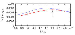
Figure 1: Temporal growth rate of the two-stream instability versus system length in a collisionless beam-plasma system. The red markers connected by the red curve represent values obtained in the simulation. The solid blue curve is calculated with the approximate formula (29). The arrow marks the length selected for fluid simulations with non-zero collision frequency shown in Figures 2 and 3.

In general, both the frequency and the wavenumber are complex numbers and functions of $L$ with band structure, as studied in detail in Ref. Kaganovich and Sydorenko, 2015. The present paper considers a single band with $3.9\leq L/\lambda_{b}\leq 4.6$. This makes the plasma size near 18 mm which is close to the size of the density plateau in the recent study of beam-plasma interaction in Ref. ?? and the size of the plasma in a dc-rf etcher considered in Ref. Xu et al., 2008. The growth rate obtained in collisionless fluid simulation for the selected band is shown by the red curve in Fig 1. Note that there is good agreement between the simulation and the approximate formula (29), compare the red and the blue curves in Fig. 1.

To study the effect of collisions with the fluid model, the value of $L=4.4\lambda_{b}$ is selected corresponding to the maximum of the collisionless growth rate marked by the arrow in Fig. 1. A set of simulations is performed with the frequency of collisions gradually increasing from zero until the growth of the amplitude of oscillations cancels completely, as shown in Fig. 2.

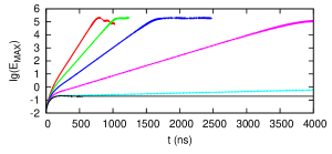
Figure 2: Logarithm of the amplitude of electric field in V/m versus time in fluid simulations with the following relative values of the collision frequency $\nu/\omega_{e,0}$: 0 (red), $0.0004$ (green), $0.0008$ (blue), $0.00119$ (magenta), $0.00146$ (cyan), and $0.00148$ (black). The dependencies are obtained at $x=4.178\lambda_{b}$. The system length is $L=4.4\lambda_{b}$, see the arrow in Figure 1.

The temporal growth rate decreases linearly with the collision frequency in good agreement with Eq. 27, compare the red and the blue curves in Fig. 1. Note that the temporal growth rate is obtained during time intervals of exponential growth with a constant rate (including the zero growth rate). One can easily identify such intervals in Fig. 2. The initial stage when the growth rate rapidly decreases with time and the saturation stage are excluded from consideration.

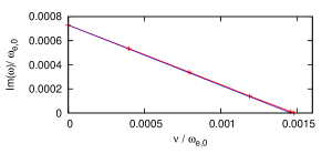
Figure 3: Temporal growth rate of the two-stream instability versus collision frequency in a finite-length beam-plasma system. The red markers connected by the red curve represent values obtained in fluid simulations. The blue curve corresponds to Eq. 27. The system length is $L=4.4\lambda_{b}$, the collisionless growth rate is marked by the arrow in Figure 1.

It is instructive to compare the results presented above with the predictions of Refs. Singhaus, 1964; Self, Shoucri, and Crawford, 1971. Equations (1) and (2) for cold beam are of no use here: the low-collision frequency limit growth rate (1) is too high and independent on the collision frequency while the expression for the high-collision frequency growth rate (2) cannot be used since the collision frequency is too low. Threshold condition for a warm beam (3), however, produces a reasonable estimate. The collision frequency which sets the growth rate to zero in the fluid simulation with $L=4.4\lambda_{b}$ above is $\nu=3.736\times 10^{7}\text{s}^{-1}$. For the selected beam and plasma parameters, according to (3), such a collision frequency cancels the instability in an infinite plasma if the beam temperature exceeds 41 eV. Similar energy spread of an 800 eV beam is observed in Ref. Xu et al., 2008. Note that using a warm electron beam reduces the growth rate of the two-stream instability even without collisions, compare equations (4) and (1). The estimate above shows that for plasma parameters used in the present paper, which are typical for plasma processing applications, the finite beam temperature and the finite system length have similar effect for a reasonable value of the beam temperature. Therefore, in future studies it is necessary to consider a finite temperature beam in a finite length plasma.

IV Kinetic simulation

In low-pressure plasmas, kinetic effects are important for the electron dynamics. The frequency of collisions with neutrals and the scattering angle for each electron depend on the electron energy. Reflection from the sheath near the wall changes the direction of the electron velocity but does not stop the particle. The electron velocity at each point is the result of action of the electric field not only in this point, but along the whole trajectory before that. These effects are omitted in the simple fluid approximation used in Section II. Therefore, it is necessary to check whether the results of the fluid theory, in particular the expressions for the growth rate (27) and the threshold current (31), remain valid if the kinetic effects are accounted for. Below, for kinetic description of the interaction of an electron beam with a low-pressure finite length plasma, a 1d3v particle-in-cell (PIC) code EDIPIC Sydorenko (2006) is used.

The PIC simulation setup is very similar to the one in the fluid simulations above: a uniform plasma is bounded by grounded walls with a distance $L$ between them and wall $x=0$ emits an electron beam with constant flux and energy. At the beginning of simulation, both beam and bulk electrons are uniformly distributed along the system. The bulk electrons and the beam electrons are represented by macroparticles with different charge which greatly improves resolution of beam dynamics for low beam currents. The ions are represented by a uniform constant immobile positively charged background which ensures quasineutrality at $t=0$. The motion of beam electrons is collisionless, they are injected at $x=0$ with the given beam energy and can freely penetrate through the boundaries. The bulk electrons may collide elastically with neutrals and are reflected specularly at the boundaries. The cross section of the collisions corresponds to Argon.

Initial plasma and beam parameters, such as $n_{e,0}$, $W_{b}$, and grid resolution $\Delta x$ are the same as in Section III. The time step is $\Delta t=1.65\times 10^{-13}\text{~{}s}$. The plasma electrons have finite initial temperature of $T_{e,0}=2\text{~{}eV}$. This value is selected as a compromise between the desire to have a cold plasma as in the fluid simulation and the growth of the numerical cost when the Debye length (and therefore the size of a cell in the computational grid) decreases for low electron temperature. Note that $T_{e,0}$ is well below the thresholds for the excitation (11.5 eV) and ionization (15.76 eV) electron-neutral collisions for Argon which justifies omitting them for the plasma electrons.

One unpleasant consequence of using plasma with a finite electron temperature is that the level of noise in PIC simulations is much higher than that in the fluid simulation. The noise, in particular, reduces time interval when the exponential growth of oscillations is visible, see Fig. 4.

Kinetic simulation reveals that the beam-plasma system is very sensitive to the length of the plasma. A set of collisionless simulations is performed with the relative beam density $\alpha=0.0001$ and $L=4.3\lambda_{b}$, $4.4\lambda_{b}$, $4.5\lambda_{b}$, and $4.6\lambda_{b}$. The selected values of $L$ correspond to the same band of the dispersion as shown in Fig. 1. Only for $L=4.5\lambda_{b}$ the exponential growth of the amplitude of oscillations has a constant rate from the start till the first amplitude maximum, see the blue curve in Fig. 4. For other values of $L$, the growth rate oscillates, see the red, green, and magenta curves in Fig. 4. Note that simulations with $L=4.4\lambda_{b}$ has a noticeable time interval where the growth rate is very close to the one in the fluid simulation with the same $L$, compare the green and the black curves in Fig. 4. It is necessary to mention that oscillations of the growth rate are observed for certain intervals of $L$ in fluid simulations as well,Kaganovich and Sydorenko (2015) but these intervals are more narrow. In view of the above, for PIC simulation with collisions described below the system length $L=4.5\lambda_{b}$ is selected.

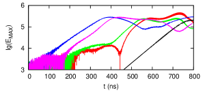
Figure 4: Logarithm of the amplitude of electric field in V/m versus time in collisionless PIC simulations with $\alpha=0.0001$ and the system length $L=4.3\lambda_{b}$ (red, obtained at $x=4.16\lambda_{b}$), $4.4\lambda_{b}$ (green, obtained at $x=4.26\lambda_{b}$), $4.5\lambda_{b}$ (blue, obtained at $x=4.31\lambda_{b}$), and $4.6\lambda_{b}$ (magenta, obtained at $x=4.36\lambda_{b}$). For comparison, the black curve represents a fluid simulation with $L=4.4\lambda_{b}$ (same as the red curve in Figure 2). Note that the blue curve corresponds to simulation 5 of Table 1.

Table 1: Parameters of PIC simulations with $L=4.5\lambda_{b}$. The neutral pressure $p_{n}$ corresponds to the given neutral gas density $n_{n}$ and the neutral gas temperature of $300\text{~{}K}$. In the growth rate column, “N/A” means that the instability is suppressed and a sufficiently long time interval with exponential growth cannot be identified.

Number	$\alpha$	$J_{b}$	$n_{n}$	$p_{n}$	$Im(\omega)$	$p_{thr}$
	($10^{-4}$)	[$\text{A/m}^{2}$]	[$10^{20}\text{~{}m}^{-3}$]	[mTorr]	[$10^{7}\text{~{}s}^{-1}$]	[mTorr]
1	0.5	26.83	0.805	2.5	0.63	8.8
2			1.61	5	0.33
3			2.415	7.5	0.08
4			3.22	10	N/A
5	1	53.67	0	0	1.41	15.2
6			1.61	5	1.01
7			3.22	10	0.38
8			4.83	15	N/A
9			6.44	20	N/A
10	1.5	80.51	3.22	10	1.34	25.0
11			4.83	15	1.01
12			6.44	20	0.5
13			8.05	25	N/A
14			9.66	30	N/A

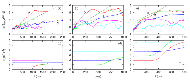
Figure 5: The logarithm of amplitude of electric field in V/m (a,c,e) and the bulk electron collision frequency (b,d,f) versus time in PIC simulations with parameters shown in Table 1. In (a) and (b), the red, green, blue, and magenta curves are for simulations 1, 2, 3, and 4 of Table 1, respectively. In (a), dashed black straight lines A, B, and C show exponential growth in simulations 1, 2, and 3, respectively. In (c) and (d), the red, green, blue, magenta, and cyan curves are for simulations 5, 6, 7, 8, and 9, respectively. In (c), dashed black straight lines D, E, and F show exponential growth in simulations 5, 6, and 7, respectively. In (e) and (f), the red, green, blue, magenta, and cyan curves are for simulations 10, 11, 12, 13, and 14, respectively. In (e), dashed black straight lines G, H, and I show exponential growth in simulations 10, 11, and 12, respectively. The growth rates for lines A to I correspond to the ones shown in Table 1.

In order to obtain a dependence of the threshold beam current on the neutral gas pressure equivalent to (31), a set of fourteen simulations is carried out with $L=4.5\lambda_{b}$, three values of electron beam density $\alpha$, and various values of neutral density $n_{n}$. The summary of these simulation parameters is given in Table 1. Note, since the threshold current (31) depends on the neutral pressure $p_{n}$, below the pressure is used instead of the density.

The behavior of the system in PIC simulations is qualitatively similar to that of the fluid system considered above. For each value of $\alpha$, the lower values of $p_{n}$ allow development of the instability with a pronounced time interval of the exponential growth with an approximately constant rate, see red, green, and blue curves in Figs. 5(a), (c), and (e). Increasing $p_{n}$ reduces the growth rate and eventually prevents oscillations from growing after a relatively short initial transitional stage which lasts no more than 200 ns, see magenta and cyan curves in Figs. 5(a), (c), and (e). The higher the value of $\alpha$, the higher is the value of $p_{n}$ which suppresses the instability.

It is necessary to mention that intense oscillations produced by the two stream instability heat plasma electrons which gradually increases the frequency of collisions, see the red and the green curves in Fig. 5(b), the green and the blue curves in Fig. 5(d), the red, green, and blue curves in Fig. 5(f). The collision frequency produced by the code diagnostics is the frequency of scattering of electrons by neutrals averaged over all electron particles. Usually the growth of the collision frequency is a clear sign that the intense oscillations are excited. Only in simulation 3 of Table 1, where the oscillations were growing at a very low rate, no significant modification of the collision frequency occurs till the end of simulation, see the blue curves in Figs. 5(a) and (b). In simulations where the prolonged exponential growth of oscillations was not identified, the collision frequency stays constant, see magenta and cyan curves in Figs. 5(b), (d), and (f). Note that the growth of the collision frequency starts when the amplitude approaches its maximum and does not affect the initial stages of the instability. The effect of the collisions on the nonlinear stage of the instability is out of the scope of this paper.

The simulation parameters are selected in such a way that for a single value of $\alpha$ there are several values of $p_{n}$. In this case, it is easier to find the threshold value of the neutral pressure $p_{n,thr}$ preventing the instability for a given beam current rather then the threshold current for a given pressure. To find the threshold pressures, the following procedure is involved. First, for each simulation where the exponential growth is observed, the growth rate is identified by fitting the dependence of the electric field amplitude versus time $E(t)$ with an exponent $\exp(Im(\omega)t)$, see the dashed black lines A-I in Figs. 5(a), (c), and (e). This gives growth rates $Im(\omega)$ for different $\alpha$ and $p_{n}$, see Table 1.

Second, values of $Im(\omega)$ from simulations with the same $\alpha$ but different $p_{n}$ are fitted with a straight line

$$Im(\omega)=Im(\omega_{ncl}^{kin})-\kappa p_{n}/2~{},$$ (32)

where $Im(\omega_{ncl}^{kin})$ has the meaning of the growth rate without collisions in the kinetic description, $\kappa$ is the coefficient of proportionality between $\nu$ and $p_{n}$ introduced in Eq. 30. In the present paper, $\kappa=1.839\times 10^{6}\text{~{}s}^{-1}\text{mTorr}^{-1}$ for electrons with a Maxwellian EVDF of temperature 2 eV performing elastic scattering in an Argon gas with temperature 300 K. This value is obtained by approximating the initial collision frequencies from simulations 6, 7, 8, and 9 of Table 1 with a linear law, as shown in Fig. 6. Equation (32) is equivalent to equation (27). Note that while the slope $\kappa/2$ of line (32) is enforced to match that of (27), the growth rates in PIC simulations fit this slope surprisingly well, compare markers with dashed straight lines of the same color in Fig. 7. The difference from the fluid theory is that the collisionless growth rates $Im(\omega_{ncl}^{kin})$ are lower than the fluid values (29) by up to to $24\%$, compare the dashed and the solid curves of the same color in Fig. 7.

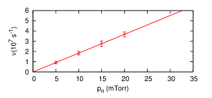
Figure 6: The average frequency of elastic electron-neutral collisions versus the neutral pressure. Markers with error bars represent values obtained in simulations 6, 7, 8, and 9 of Table 1, the error bars correspond to the amplitude of noise in the simulation. The solid line is described by equation (30) with $\kappa=1.839\times 10^{6}\text{~{}s}^{-1}\text{mTorr}^{-1}$.

Finally, with $Im(\omega_{ncl}^{kin})$ known for each $\alpha$, the threshold pressure values giving $Im(\omega)=0$ are calculated as

$$p_{n,thr}=2Im(\omega_{ncl}^{kin})/\kappa~{},$$ (33)

which is equivalent to (28). These threshold pressures are given in Table 1 and are marked by arrows in Fig. 7.

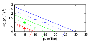
Figure 7: Temporal growth rate of the two-stream instability versus the neutral gas pressure. The solid straight lines are obtained with fluid theory equations (27) and (29) where $\nu_{e}(p_{n})$ is defined by equation (30); the red, green, and blue solid lines are for $\alpha=5\times 10^{-5}$, $10^{-4}$, and $1.5\times 10^{-4}$, respectively. Red markers represent simulations 1, 2, and 3 of Table 1, respectively (see also lines A, B, and C in Fig. 5(a)). Green markers represent simulations 5, 6, and 7 of Table 1, respectively (see also lines D, E, and F in Fig. 5(c)). Blue markers represent simulations 10, 11, and 12 of Table 1, respectively (see also lines G, H, and I in Fig. 5(e)). Dashed red, green, and blue straight lines are the approximate dependencies “growth rate versus pressure” for $\alpha=5\times 10^{-5}$, $10^{-4}$, and $1.5\times 10^{-4}$, respectively, plotted as the best fit of the PIC simulation data. The arrows mark threshold pressures which turn the growth rate of the instability into zero for the three values of the beam density mentioned above.

The three values of $p_{n,thr}$ for the three values of beam current (shown by open black markers connected by a solid black line in Fig. 8) are fitted with a linear law

$$J_{b,thr}^{kin}=3.4p_{n}$$ (34)

shown by the black dashed straight line in Fig. 8. In (34), the current density is in $\text{A}/\text{m}^{2}$ and the neutral pressure is in mTorr. This curve represents the threshold current predicted by the PIC simulation. For comparison, with $\kappa$, $W_{b,0}$, $n_{e,0}$, and $L_{n}$ as in the kinetic simulations with $L=4.5\lambda_{b}$ above, the fluid threshold current (31) is

$$J_{b,thr}=2.695p_{n}~{},$$ (35)

where the current density and the pressure units are the same as in (34). Thus, for the same pressure, the value of the threshold current predicted by PIC simulations is about $26\%$ higher than the value given by the fluid theory, compare the dashed black and the solid magenta lines in Fig. 8. This difference corresponds to the lower collisionless growth rates in kinetic simulation which is reasonable since kinetic effects have a tendency to disrupt the resonance between the wave and the particles and reduce the growth rate. Overall, for the selected parameters there is a very reasonable agreement between the kinetic simulations and the simple fluid theory given in Section II.

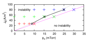
Figure 8: Phase plane “emission current density vs neutral gas pressure”. Red markers in ascending pressure order represent simulations 1, 2, 3, and 4 of Table 1, respectively. Green markers in ascending pressure order represent simulations 5, 6, 7, 8, and 9, respectively. Blue markers in ascending pressure order represent simulations 10, 11, 12, 13, and 14, respectively. Everywhere, the vertical crosses mark simulations where the exponential growth is identified while the diagonal crosses mark simulations where the instability is suppressed. Open boxes connected by a solid black line represent threshold pressures given in Table 1 and marked by arrows in Fig. 7. The dashed black straight line is the threshold current (34) plotted using these threshold pressure values. The solid magenta line is the threshold curent (35) calculated using the fluid theory.

V Summary

The two-stream instability in a plasma bounded between walls is quite different from that in an infinite plasma. The oscillations grow both in time and space, and the growth rates are functions of the distance between the bounding walls. If this distance is only few resonance wavelengths, the temporal growth rate is very small. Scattering of plasma bulk electrons further reduces this growth rate. The present paper finds that the rate becomes zero if the collision frequency is equal to the doubled growth rate without collisions. Unlike the results of previous studies,Singhaus (1964); Self, Shoucri, and Crawford (1971) this criterion predicts that the instability may be completely suppressed for cold beams. The proposed fluid theory allows to calculate a threshold beam current density for the given neutral gas pressure $p_{n}$, the collision frequency as a function of the pressure $\nu_{e}=\kappa p_{n}$, the electron density $n_{e}$, the beam energy $W_{b}$, and the normalized system length $L_{n}$:

$$J_{b,thr}=\frac{6.5\kappa\sqrt{2e\varepsilon_{0}n_{e}W_{b}}}{L_{n}\ln(L_{n})\left[1-0.18\cos\left(L_{n}+{\pi}/{2}\right)\right]}p_{n}~{},$$

where $W_{b}$ is in electronvolts while the units of $p_{n}$ depend on the method of calculation of the coefficient $\kappa$. The instability will not develop if the beam current is below this threshold. The quantitative effect of collisions on both the growth rate and the threshold current predicted by the fluid theory is in good agreement with the results of kinetic simulations.

References

- Xu et al. (2008) L. Xu, L. Chen, M. Funk, A. Ranjan, M. Hummel, R. Bravenec, R. Sundararajan, D. J. Economou, and V. M. Donnelly, Appl. Phys. Lett. 93, 261502 (2008).
- Sato and Heider (1975) M. Sato and J. Heider, J. Phys. D: Appl. Phys. 8, 1632 (1975).
- Singhaus (1964) H. E. Singhaus, Phys. Fluids 7, 1534 (1964), doi: 10.1063/1.1711408.
- Self, Shoucri, and Crawford (1971) S. A. Self, M. M. Shoucri, and F. W. Crawford, J. Appl. Phys. 42, 704 (1971).
- Abe et al. (1979) H. Abe, O. Fukumasa, R. Itatani, and H. Naitou, Phys. Fluids 22, 310 (1979), doi: 10.1063/1.862582.
- Dawson (1964) J. M. Dawson, Phys. Fluids 7, 419 (1964), doi: 10.1063/1.1711214.
- Lewis, Sykes, and Wesson (1972) H. R. Lewis, A. Sykes, and J. A. Wesson, J. Comp. Phys. 10, 85 (1972).