Fuzzy c-Shape: A new algorithm for clustering finite time series waveforms

Abstract

The existence of large volumes of time series data in many applications has motivated data miners to investigate specialized methods for mining time series data. Clustering is a popular data mining method due to its powerful exploratory nature and its usefulness as a preprocessing step for other data mining techniques. This article develops two novel clustering algorithms for time series data that are extensions of a crisp c-shapes algorithm. The two new algorithms are heuristic derivatives of fuzzy c-means (FCM). Fuzzy c-Shapes plus (FCS+) replaces the inner product norm in the FCM model with a shape-based distance function. Fuzzy c-Shapes double plus (FCS++) uses the shape-based distance, and also replaces the FCM cluster centers with shape-extracted prototypes. Numerical experiments on 48 real time series data sets show that the two new algorithms outperform state-of-the-art shape-based clustering algorithms in terms of accuracy and efficiency. Four external cluster validity indices (the Rand index, Adjusted Rand Index, Variation of Information, and Normalized Mutual Information) are used to match candidate partitions generated by each of the studied algorithms. All four indices agree that for these finite waveform data sets, FCS++ gives a small improvement over FCS+, and in turn, FCS+ is better than the original crisp c-shapes method. Finally, we apply two tests of statistical significance to the three algorithms. The Wilcoxon and Friedman statistics both rank the three algorithms in exactly the same way as the four cluster validity indices.

I Introduction

Increasing, large volumes of time series data are becoming available from a diverse range of sources, including smart phones, environmental sensors and biological devices. Techniques for analyzing time series data include dimensionality reduction [jadid15], indexing [2],[3], and segmentation [jadid16]. In addition, techniques have been developed to extract the underlying shape or trends in the data, for tasks such as pattern discovery [4, 5, 6], classification[7, 8], rule discovery and summarization. An open challenge in time series analysis is how to cluster a set of time series according to the similarity of their underlying shape. The basic objective of this article is to generalize the fuzzy c-means (FCM) model [1] to accommodate clustering in finite time series data.
In general, clustering is an analytic tool that can identify interesting patterns and correlation in the underlying data [9]. For example in ECG signals the goal may be to cluster the ECG signals so that normal heart signals can be distinguished from abnormal signals based on the shape and phase of the time series signals. A key problem in finite time series clustering is the choice of an appropriate distance measure, which can be used to analyze the similarities/dissimilarities of finite time series. Such a distance measure should be able to address questions such as: (i) how to describe the underlying shape or trend in the time series? and (ii) how to handle distortion in the amplitude and phase of the time series, such as noise or jitter?
Among different distance measurement methods that have been used for time series clustering, Euclidean distance (ED) and Dynamic Time Warping (DTW) are the most popular methods. In most of clustering techniques for time series data, Euclidean distance is used for measuring the similarities/dissimilarities of time series. However, this distance is most useful when we have time series in the form of equal length records. Euclidean distance in time series clustering only compares the points of the time series in a fixed order, so it cannot be used for clustering time series with time shifts. The DTW distance can be used for evaluating similarities/dissimilarities of time series data based on their shape information. However, this method is computationally expensive, since the cost of computing the similarity/dissimilarity between each pair of time series is quadratic in the length of the records.
Most state-of-the-art approaches for shape-based clustering suffer from two main drawbacks: (i) they are computationally expensive and thus, not suitable for large volumes of data [6, 10, 5, 11]; and (ii) these approaches are limited to specific domains [11], or their effectiveness has only been evaluated over a small number of datasets [6, 10].
k-Shape [12] is a novel method that has been proposed to address the problem of finding a suitable distance measure and clustering method for finite time series data, where time series sequences belong to the same cluster, exhibiting similar patterns, regardless of differences in amplitude and phase. Paparizos and Gravano [12] select a statistical measure, cross-correlation, as a shape similarity distance measure for comparing time series sequences. For clustering time series data, they modify the classical crisp k-means clustering algorithm (also called hard c-means (HCM)) with a new centroid computation technique based on a shape extraction method while computing the clusters. These two novel modifications seem highly effective in terms of clustering accuracy and efficiency. To demonstrate the robustness of k-Shape clustering [12], the authors perform an extensive evaluation over 48 different time series datasets and demonstrate the superiority of their technique against fifteen existing schemes.
In this paper, we introduce two novel clustering algorithms. The first substitutes the Shape Based Distance (SBD) measure introduced in [12] for the model norm in the standard fuzzy c-means [13] algorithm, and the second uses the SBD measure and shape extraction method in [12] to update prototypes in the fuzzy c-means clustering algorithm [13]. These two modifications result in $\displaystyle 4.5\%$ and $\displaystyle 58.5\%$ improvement respectively in accuracy and efficiency in comparison to k-Shape clustering. We make a direct comparison with the results reported in the k-Shape paper, by evaluating our methods on the same UCR time series classification archive [14], which consists of 48 labeled time series datasets from various real-world domains.
The rest of the paper is organized as follows: Section II reviews related work on time series clustering, Section III presents the relevant theoretical background on fuzzy c-means and k-Shape clustering that are based of our two new algorithms. Section IV introduces our two novel clustering methods FCS++ and FCS+. Section V discusses the four external cluster validity indices used for measuring the accuracy of clustering methods. Section VI evaluates our proposed methods with extensive numerical experiments, and shows that our algorithms outperform the crisp k-Shape clustering algorithm in terms of accuracy and efficiency. Sections VII and Section VIII contain a short discussion of our conclusions and some future research directions.

II Related Work

Among different techniques for analyzing time series data, clustering is a popular data mining method due to its usefulness as a preprocessing step for other data mining techniques. There are comprehensive literature surveys on time series clustering such as[15, 16, 17]. Generally time series clustering algorithms fall in to two categories: Statistical-based and shape-based methods. Statistical-based methods, use characteristic measures [18], varying coefficient models [19], and subsequences of time series as approaches for extracting features to cluster time series data. However, there are two general drawbacks of using these methods: first, applying these methods usually leads to trial and error problems because of their requirement for adjusting multiple parameters; second, they are not domain-independent [12]. On the other hand, shape-based methods do not have these limitations and they have been used in a variety of studies. Therefore, in this paper we focus on shape-based clustering. In the following we briefly review shape-based distance functions for time series data as well as relevant clustering techniques that have been reported in the literature.
An efficient shape-based distance function that measures the similarities/dissimilarities between time series data, should not be sensitive to the time of appearance of similar sequences [17]. Indeed, a distance function that measures the shape similarity should be invariant to phase and amplitude. Therefore, elastic methods [20, 21] like DTW [22] are more suitable for shape-based time series clustering.
Next, we review relevant shape-based distance functions that have been introduced in previous studies. In [23] the authors introduced an indexing method using Euclidean distance in a lock-step measurement (one-to-one) manner. Sensitivity to scaling is the drawback of this method. The DTW distance has better accuracy but lower efficiency than this method. In [24] the authors proposed a cross-correlation based distance function that is very efficient for noise reduction. In addition, this distance function can summarize the temporal structure of the time series data. In [25, 26] a non-metric similarity measure is proposed based on the Longest Common Sub-Sequence (LCSS), which has very good noise robustness. In this method, the similarity between trajectories is considered by giving more weight to similar segments of the sequences.
In [27] the Edit Distance with Real Penalty (ERP) is introduced as a metric that can handle local shifting in time series data. The ERP approach is a robust method against noise and is shift- and scale-invariant. In [28] the Minimal Variance Matching (MVM) method is proposed which is able to skip outliers automatically. MVM uses the DTW method for calculating the similarity between two time series, but MVM, unlike DTW, can skip some target series. In addition, MVM, like the LCSS method, can allow the query sequences to match to only sub-sequence of the target sequence.
In [29] the authors introduced the Edit Distance on Real sequence (EDR) method, which is robust against noise, shifts, and scaling of the time series data. This method is more robust than the ED, DTW, and ERP methods, and it is outperforms the LCSS method. EDR measures the similarity between two trajectories based on the edit distance on strings. By assigning penalties to the unmatched segments, EDR improves its accuracy, and by quantizing the distance between 0 and 1 effectively removes the noise. In [30] the Sequence Weighted Alignment (Swale) model is proposed to score similarities between time series data based on rewards for matching portions, and penalties for mismatching portion of sequences.
In [15, 31] the authors conducted extensive experiments on 38 data sets from a wide variety of application domains to compare distance functions. They concluded that the constrained Dynamic Time Warping (cDTW) method [32] outperforms all other distance measurement methods in term of accuracy.
The Shape Based Distance (SBD) [12] is a novel measurement approach that handles distortions in amplitude and phase accurately, by efficiently using cross-correlation through normalization of a shape-based distance measure. According to the authors of [12], SBD achieves similar accuracy to cDTW but it does not require any tuning, and it is an order of magnitude faster. In this paper we use SBD as the distance function in our algorithms.
Many studies have focused on partitional models of clustering using a shape-based distance function that is shift- and scale-invariant. Among partitional clustering methods, k-medoids [33] clustering has been used widely because of its ease of incorporating a shape-based distance measure [15, 31]. However, k-medoids is a computationally expensive and non-scalable method. Alternatively, other studies [6, 10, 5, 11] have focused on k-means (aka hard c-means (HCM)) [34] with various choices of centroid computation and/or distance measure. The best performing k-means approaches have used DTW while proposing a new centroid extraction method[6, 10, 5, 11, 12].
Recently, a novel partitional clustering algorithm, k-Shape, that uses the SBD distance, was proposed in [12]. The k-Shape algorithm preserves the shapes of time series when comparing them, and computes centroids in a scale- and phase- invariant way. The authors of [12] showed that k-Shape partitioning of 48 finite, labeled time series data sets was superior to 15 other methods based on spectral, partitional, and hierarchical clustering approaches. k-Shape appears to be a scalable and accurate approach for time series clustering that can be applied to a wide variety of domains.
There are also fuzzy approaches to clustering in time series based on algorithms such as FCM. Studies based on fuzzy clustering of time series data include [35, 24, 36]. In [35] a short time series (STS) distance is proposed to measure similarities between time series that are short in length, based on their shape. By changing the Euclidean distance to STS distance in the standard fuzzy c-means algorithm, they modified the membership matrix and centroid computation algorithm, thus producing a fuzzy time series clustering algorithm for short time series data. In [24] the cross-correlation method is considered as the distance measure in the fuzzy c-means clustering algorithm and arithmetic means are used for prototype computation to cluster functional MRI data. The authors in [37] used the DTW method as distance measure and applied k-means and c-medoids algorithms as clustering methods. Comparing the results of these two methods, led them to conclude that k-means cannot produce satisfactory results whereas c-medoids obtained good accuracy. In this paper, we propose two novel shape-based clustering methods of time series data based on heuristic derivatives of FCM.

III Preliminaries

Many clustering algorithms exist for numerical feature vector data such as $\displaystyle X=\{x_{1},x_{2},\dots,x_{n}\}\subset\Re^{p}$. There are three basic problems associated with clustering in $\displaystyle X:$ $\displaystyle(i)$ pre-clustering assessment of tendency (what value of c, the number of clusters, to use?); $\displaystyle(ii)$ partitioning the data (finding the c clusters); and $\displaystyle(iii)$ post-clustering validation (are the clusters useful, realistic, etc.?). Good presentations on each of the three basic problems include the general texts [38, 39, 1, 40]. This study concerns itself with three algorithms for clustering in data where each $\displaystyle x_{k}\in X$ is a vector of length $\displaystyle p$ that represents a finite portion of a waveform or time series. Data of this type are prevalent in many fields: for example, stock market analysis [41], satellite imagery [42], computational finance [43] and neuroscience, [44, 45, 46].
In this section we review the relevant theoretical background for our new clustering algorithms. In Section  III-A, we review fuzzy c-means clustering, which is the basis of our work. In Section  III-B, we introduce the shape-based distance (SBD) [12]. Section  III-C introduces a new method for assigning a center to clusters based on the shape of the time series and briefly explains the k-Shape clustering method[12].

III-A The Generalized Fuzzy c-Means Model

Crisp and fuzzy/probabilistic c-partitions of $\displaystyle n$ objects are, respectively, the sets of matrices defined as

$$\displaystyle M_{fcn}=\{U\in\Re^{cn}:for\,1\leq i\leq c,1\leq k\leq n;0\leq u_{ik}\leq 1;$$

$$\displaystyle\qquad\displaystyle\sum_{i=1}^{c}u_{ik}=1\,\,\forall k;\,\displaystyle\sum_{k=1}^{n}u_{ik}>0\,\,\forall i\}$$ (1a)

$$\displaystyle\qquad M_{hcn}=\{U\in M_{fcn}:u_{ik}\in\{0,1\}\forall i,k\}.$$ (1b)

The Generalized Least Squares Error (GLSE) clustering model is the constrained optimization problem

$$\displaystyle min_{(U,P)}\{J_{m}(U,P;X)=\displaystyle\sum_{k=1}^{n}\displaystyle\sum_{i=1}^{c}(u_{ik})^{m}[\Delta(x_{k},p_{i})]^{2}\}.$$ (2)

In equation (2), $\displaystyle m$ is a weighting parameter, $\displaystyle m\geq 1$, $\displaystyle U\in M_{fcn}$, $\displaystyle P=\{p_{1},\dots,p_{c}\}$ is a set of cluster prototypes, and $\displaystyle[\Delta(x_{k},p_{i})]^{2}$ is a measure of the squared error incurred by representing input $\displaystyle x_{k}$ by prototype $\displaystyle p_{i}$. Optimal partitions $\displaystyle U^{*}$ of $\displaystyle X$ are taken from pairs $\displaystyle(U^{*},V^{*})$ that are local minimizers of $\displaystyle J_{m}$.
There are dozens of instances of equation (2) for specific choices of $\displaystyle P$ and $\displaystyle\Delta$. For example, the prototypes $\displaystyle P$ may be points, lines, planes, linear varieties [1], hyperquadrics [47], or even regression functions [48]. The dissimilarity measure $\displaystyle\Delta$ may be an inner product norm [1], a Minkowski norm [49], or a shape-based distance [12] such as the one used in this paper.
For many choices of $\displaystyle(P,\Delta)$, there is a theory to guide approximate solutions of the model in equation (2) by an alternating optimization $\displaystyle(AO)$ algorithm based on Picard iteration through necessary conditions for its local extrema. The most familiar case is the original fuzzy c-means (FCM) model with accompanying FCM/AO algorithm, first reported in [13] and described at length in [1]. This case is covered by:

Theorem (1) (FCM)[13]: Let $\displaystyle X=\{x_{1},\dots,x_{n}\}\subset\Re^{p}$ contain at least $\displaystyle c$ distinct points. Let $\displaystyle P=V=\{v_{1},\dots,v_{c}\}\subset\Re^{p}$, and $\displaystyle A$ be a positive-definite norm inducing $\displaystyle p\times p$ weight matrix, $\displaystyle\Delta(x_{k},p_{i})^{2}=\|x_{k}-v_{i}\|_{A}^{2}=(x_{k}-v_{i})^{T}A(x_{k}-v_{i})>0\quad\forall i,k$. If $\displaystyle m>1$, then $\displaystyle(U,V)\in M_{fcn}\times\Re^{p}$ may minimize $\displaystyle J_{m}(U,V;X)$ only if

$$\displaystyle u_{ik}=\left(\displaystyle\sum_{j=1}^{c}\left(\frac{\|x_{k}-v_{i}\|_{A}}{\|x_{k}-v_{j}\|_{A}}\right)^{\frac{2}{m-1}}\right)^{-1};1\leq i\leq c;1\leq k\leq n,$$ (3a)

$$\displaystyle v_{i}=\displaystyle\sum_{k=1}^{n}u_{ik}^{m}x_{k}/\displaystyle\sum_{k=1}^{n}u_{ik}^{m};\,1\leq i\leq c.$$ (3b)

It is also well known that when $\displaystyle m=1$ the partition matrix $\displaystyle U$ is necessarily crisp, $\displaystyle U\in M_{hcn}$, and under the remaining hypotheses in Theorem (1), that equation (2) reduces to the classical hard c-means (HCM, or classical k-means) model which was first discussed by Lloyd in [50]. In this case, there are several ways to show that conditions (3) reduce to the following well known necessary conditions for minimizing $\displaystyle J_{1}$.

Theorem (2) (HCM) [13] : Let $\displaystyle X=\{x_{1},\dots,x_{n}\}\subset\Re^{p}$ contain at least $\displaystyle c$ distinct points, $\displaystyle P=V=\{v_{1},\dots,v_{c}\}\subset\Re^{cp}$ , and $\displaystyle m=1$. If $\displaystyle\Delta(x_{k},p_{i})^{2}=\|x_{k}-v_{i}\|_{A}^{2}>0\quad\forall i,k$, then $\displaystyle(U,V)\in M_{fcn}\times\Re^{cp}$ may minimize $\displaystyle J_{1}(U,V;X)$ only if $\displaystyle U\in M_{hcn}$ is a hard c-partition of $\displaystyle X$, and

$$\displaystyle u_{ik}=\begin{Bmatrix}1&\quad\|x_{k}-v_{i}\|_{A}<\|x_{k}-v_{j}\|_{A}\forall j\neq i\\ 0&\quad\text{otherwise }\\ \end{Bmatrix}$$ (4a)

$$\displaystyle v_{i}=\displaystyle\sum_{k=1}^{n}u_{ik}x_{k}/\displaystyle\sum_{k=1}^{n}u_{ik};\,1\leq i\leq c\,\,$$ (4b)

The content of Theorem (2) is often given by denoting the partition $\displaystyle U\in M_{hcn}$ by its equivalent set-theoretic form,
$\displaystyle X=\bigcup_{i=1}^{c}X_{i}$; $\displaystyle\oslash=X_{i}\bigcap_{i\neq j}X_{j}$; $\displaystyle\displaystyle\sum_{i=1}^{c}\mid X_{i}\mid=\displaystyle\sum_{i=1}^{c}n_{i}=n$. Using this representation, equations (4) take the alternate form

$$\displaystyle u_{ik}=\begin{Bmatrix}1&\quad x_{k}\in X_{i}\\ 0&\quad\text{otherwise }\\ \end{Bmatrix};1\leq i\leq c,\,1\leq k\leq n$$ (5a)

$$\displaystyle v_{i}=\bar{v}_{i}=\displaystyle\sum_{x_{k}\in X_{i}}\left(\frac{x_{k}}{n_{i}}\right);1\leq i\leq c.$$ (5b)

The advantage of using equations (4) instead of (5) is that the role of the partition matrix $\displaystyle U$ is clearly seen in the more general fuzzy case. Note that (5a) labels each point in $\displaystyle X$ with the nearest prototype rule; and (5b) shows that the point prototypes are none other than the geometric centroids (sample means) of the $\displaystyle c$ clusters in $\displaystyle X$.
There are various ways to estimate solutions for the GLSE problem (2) for the choice $\displaystyle[\Delta(x_{k},p_{i})]^{2}=\|x_{k}-v_{i}\|_{A}^{2}$. The most popular method is Picard iteration through necessary conditions (3) or (4). For the fuzzy case, these are first order necessary conditions (FONCs, the gradient must vanish at extreme points). For the crisp case, looping through conditions (4) or (5) is sometimes called Lloyd iteration: (4b), (5b) is a FONC, and (4a), (5a) is necessary, but not first order. This method is summarized as Algorithm 1.

Algorithm 1 AO c-means for HCM and FCM

0:   $\displaystyle X=\{x_{1},\dots,x_{n}\}\subset\Re^{p}$

0:  $\displaystyle(U,V)$

1:  Pick  $\displaystyle 1<c<n:m\geq 1$ $\displaystyle T_{M}=iterationLimit$

2:  Model Norm: $\displaystyle\parallel x-v\parallel_{A}=\sqrt{(x-v)^{T}A(x-v)}$

3:  $\displaystyle E_{t}=\mid J_{m}(U_{t},V_{t})-J_{m}(U_{t-1},V_{t-1})\mid$

4:  $\displaystyle 0<\varepsilon=terminationCriteria$

5:  Guess  $\displaystyle V_{0}=\{v_{10},\dots,v_{c0}\}\subset\Re^{cp}$

6:  Calculate $\displaystyle U_{0}$ with $\displaystyle V_{0}$ and (3a) or (4a)

7:  $\displaystyle t=1$: $\displaystyle E_{1}=bigNumber$

8:  while $\displaystyle t<T_{m}\quad and\quad E_{t}>\varepsilon$ do

9:     Calculate $\displaystyle U_{t}$ with $\displaystyle V_{t-1}$ and (3a) or (4a)

10:     Calculate $\displaystyle V_{t}$ with (3b) or (4b)

11:     $\displaystyle t=t+1$

12:  end while

13:  $\displaystyle(U,V)\leftarrow(U_{t},V_{t})$

Reference [1] contains details about most of the issues that arise concerning the use of these two clustering models and Algorithm 1. Our interest is confined to three algorithms for clustering finite time series in the special case when each $\displaystyle x_{k}\in X$ is a vector of length $\displaystyle p$ that represents a finite portion of a waveform or time series. All three algorithms are ad hoc methods that depend on equations (4) or (5) and use Algorithm 1 with appropriate modifications to find approximate solutions.

III-B Shape Based Distance

The quality of clustering in feature vector data almost always depends on finding a good way to measure similarity or distance between the items represented by the data. Waveform data presents some special challenges, when represented by fixed length vectors of finite time series. Most of the extant literature on clustering in time series data modifies a classic clustering algorithm such as k-means by (i) substituting a suitable distance measure on the raw data; or (ii) by extracting features from the data that convert it into vectors that can be inserted directly into a classic algorithm. This paper follows the approach taken in [12], which concentrates attention on SBD as the distance of choice for waveform clustering.
The underlying desire in waveform clustering is to use a distance measure that capture shapes differences that are invariant to phase and amplitude changes in the data. Constrained dynamic time warping is often recommended for this job [32]. Forty six (46) such measures for time series data are discussed in [51]! This gives some idea of how long and hard the path towards a good waveform distance measure has been. The shape-based distance (SBD) measure introduced in [12] for time series data forms the basis for our two new algorithms.
The new algorithms begin by modifying the GLSE model at (2) by introducing the SBD, which is tailored to the time series case to define $\displaystyle\Delta(x_{k},p_{i})$. Specifically, this distance is introduced for a pair of z-normalized vectors $\displaystyle x$ and $\displaystyle y$ of length $\displaystyle p$ in Algorithm 2:

Algorithm 2 [12]: $\displaystyle[dist,y^{\prime}]=SBD(x,y)$

0:  Two z-normalized sequences $\displaystyle x,y\in\Re^{p}$

0:  Dissimilarity dist = SBD(x,y) $\displaystyle\in\Re^{+}$;Aligned sequence y’ of y towards x

1:  length = $\displaystyle 2^{nextpower2(2*length(x)-1)}$

2:  $\displaystyle CC=IFFT\{FFT(x,length)^{*}FFT(y,length)\}$%(A)

3:  $\displaystyle NCC_{c}=CC/\parallel x\parallel\bullet\parallel y\parallel$

4:  [value,index] = max($\displaystyle NCC_{c}$)

5:  dist= 1 - value               % (B)

6:  shift = index - length(x)

7:  if $\displaystyle shift\geq 0$ then

8:     y’= [zeros(1,shift), y(1:end-shift)]      %(C)

9:  else

10:     y’= [y(1-shift:end), zeros(1,-shift)]      %(C)

11:  end if

Notes about Algorithm 2 The z-normalization mentioned in the input line is the standard $\displaystyle(0,1)$ statistical normalization, i.e., the $\displaystyle n$ input vectors are linearly transformed by subtracting their feature means and dividing by their standard deviations for each of the $\displaystyle p$ features in the input data. Lines $\displaystyle 2$, $\displaystyle 5$, and $\displaystyle 8$ correspond to the following equations from [12].
$\displaystyle(A)$ $\displaystyle CC(X,Y)=\mathcal{F}^{-1}\{\mathcal{F}(x)^{*}\mathcal{F}(y)\}$, where $\displaystyle\mathcal{F}$ and $\displaystyle\mathcal{F}^{-1}$ are forward (inverse) discrete Fourier transforms, $\displaystyle*$ is convolution.
$\displaystyle(B)$ $\displaystyle dist=SBD(x,y)=1-max_{w}\{CC_{w}(x,y)/\|x\|\bullet\|y\|\}$, where $\displaystyle w\in\{1,2,\dots,2p-1\}$; $\displaystyle CC_{w}(x,y)=R_{w-p}(x,y)$; and

$\displaystyle R_{k}(x,y)=\begin{Bmatrix}\displaystyle\sum_{j=1}^{p-k}x_{j+k}y_{j};&\quad k\geq 0\\ R_{-k}(x,y);&\quad k<0\\ \end{Bmatrix}$.
$\displaystyle(C)$ $\displaystyle x_{(s)}=\begin{Bmatrix}(\overbrace{0,\dots,0}^{\mid s\mid},x_{1},\dots,x_{p-s});&\quad s\geq 0\\ (x_{1-s},\dots,x_{p},\underbrace{0,\dots,0}_{\mid s\mid});&\quad s<0\\ \end{Bmatrix}$.

Equation $\displaystyle(C)$ shows how a sliding window passes across a vector, while looking for the optimal alignment between $\displaystyle x$ and $\displaystyle y$. The inputs to Algorithm 2 are vectors in $\displaystyle\Re^{p}$, so the distance $\displaystyle\|x_{k}-v_{i}\|_{A}$ in equations (4a) and (5a) can be directly replaced by $\displaystyle SBD(x,y)$, which is called a distance in [12]. Since $\displaystyle SBD(x,y)$ is produced by Algorithm 2, it is not immediately obvious whether the function $\displaystyle\Delta=SBD$ is really a metric on $\displaystyle\Re^{p}$. Moreover, it is not clear whether the distance emerging from Algorithm 2 should be regarded as a squared distance or not, although the authors of [12] state that it replaces $\displaystyle[\Delta(x,v)]^{2}$ in the GLSE problem. The authors of [12] make this substitution in (4a) and in line 3 of Algorithm 1 with $\displaystyle m=1$, and call the resultant algorithm the $\displaystyle k-AVG+ED$ algorithm, where $\displaystyle AVG$ means (4b) or (5b) is used to compute the prototype updates, and $\displaystyle ED$ stands for Euclidean distance.
Paparrizos and Gravano argue in [12] that most of the research on waveform clustering has used distances like DTW to the exclusion of cross correlation $\displaystyle(CC)$ between time series because this time honored statistical method suffers from normalization and registration issues. They assert that to be useful, the data and the $\displaystyle CC$ applied to it must be appropriately normalized. The z-normalization of the inputs to Algorithm 2 gives it scale invariance, and takes care of inherent distortion in the data. They tackle the normalization of $\displaystyle CC$ with equations (A)-(C) that follow Algorithm 2. Shift invariance is addressed by computing $\displaystyle CC_{w}(x,y)=R_{w-p}(x,y)$, which maximizes $\displaystyle CC$ at the best match between $\displaystyle x$ and $\displaystyle y$ by testing each position offered by the sliding window in equation (C). They discuss three ways to normalize $\displaystyle CC$, but only use $\displaystyle CC_{w}$, shown and used here, which produces values in the closed interval $\displaystyle[-1,1]$. Consequently, $\displaystyle SBD(x,y)\in[0,2]$, and it takes the value $\displaystyle 0$ when $\displaystyle x$ and $\displaystyle y$ are perfectly similar (corresponding to zero distance, i.e., $\displaystyle x=y$). Efficiency of finding $\displaystyle CC_{w}$ is addressed by using the discrete forward and inverse Fourier transforms and padding the input data so its length is always a power of $\displaystyle 2$. The overall complexity of Algorithm 2 is given as $\displaystyle O(plog(p))$.

III-C Shape Based Prototypes and k-Shape Clustering

The second major alteration of k-means introduced in [12] is to compute prototypes that attempt to capture shape information, based on the fact that input vectors represent finite time series waveforms. To begin, we revisit equation (3a) for $\displaystyle v_{i}$. This prototype arises for FCM by zeroing the gradient of the function $\displaystyle J_{m}(U^{*},V;X)$ in the reduced optimization problem

$$\displaystyle min_{V\in\Re^{cp}}\left\{J_{m}(U^{*},V;X)=\displaystyle\sum_{k=1}^{n}\displaystyle\sum_{i=1}^{c}(u_{ik}^{*})^{m}\|x_{k}-v_{i}\|_{A}^{2}\right\}.$$ (6)

$\displaystyle U^{*}$ is fixed in (6), and minimization of $\displaystyle J_{m}(U^{*},V;X)$ is unconstrained, so solving $\displaystyle\nabla_{v_{i}}J_{m}(U^{*},V;X)=0$ for $\displaystyle v_{i}$ leads directly to (3a) in the fuzzy case, and (4a) in the crisp case. When the distance in equation (6) is not an inner product norm, $\displaystyle J_{m}(U^{*},V;X)$ is generally not differentiable with respect to $\displaystyle v_{i}$. In this more general case, the reduced problem for the crisp case ($\displaystyle m=1$ in (6)) of the GLSE model becomes:

$$\displaystyle min_{v\in\Re^{p}}\left\{J_{1}(v;X)=\displaystyle\sum_{x_{k}\in X_{i}}\Delta(x_{k}-v)^{2}\right\}.$$ (7)

The method of solving (7), sometimes referred to as the Steiner sequence problem [52], depends on the nature of the distance function $\displaystyle\Delta(x_{k}-v)$. When alignment of the observations $\displaystyle\{x_{k}\}$ with prototype $\displaystyle v$ is required, this becomes the multiple sequence alignment problem, known to be NP-complete [53]. Bypassing some intermediate steps given in [12], (7) eventually becomes an instance of maximization of the famous Rayleigh Quotient [38], viz,

$$\displaystyle v_{i}=max_{v\in\Re^{p}}\left\{\frac{v^{T}Q^{T}SQV}{v^{T}v}\right\}=max_{v\in\Re^{p}}\left\{\frac{v^{T}Mv}{v^{T}v}\right\}$$ (8)

where $\displaystyle M=Q^{T}SQ$, $\displaystyle Q=I-(1/p)[$1$\displaystyle]$, and $\displaystyle[$1$\displaystyle]$ is the $\displaystyle p\times p$ matrix of $\displaystyle 1^{\prime}s$. The solution of (8) is the eigenvector corresponding to the largest eigenvalue of the real symmetric matrix $\displaystyle M$, which is computed in the last line of Algorithm 3, which records this procedure as shown in [12].

Algorithm 3 [12]: $\displaystyle V_{i,t+1}$= Shape Extraction($\displaystyle X,v_{i,t}$)

0:  $\displaystyle X=\{x_{1},\dots,x_{n}\}\subset\Re^{p}$ as a $\displaystyle n\times p$ matrix $\displaystyle X$ whose columns are z-normalized time series vectors. $\displaystyle v_{i,t}\in\Re^{p}$ is the reference sequence against which time series of $\displaystyle X$ are aligned

0:  $\displaystyle v_{i,t}\in\Re^{p}$      % new $\displaystyle i^{th}$ shape prototype

1:  $\displaystyle X^{\prime}\leftarrow$ $\displaystyle[\quad]$

2:  for $\displaystyle i=1$ to $\displaystyle n$ do

3:    [dist,$\displaystyle x^{\prime}$] $\displaystyle\leftarrow$ SBD($\displaystyle v_{i,t},X(i)$)  %Algorithm 2

4:    $\displaystyle X^{\prime}$ $\displaystyle\leftarrow$ $\displaystyle[X^{\prime};x^{\prime}]$

5:  end for

6:    $\displaystyle S$ $\displaystyle\leftarrow$ $\displaystyle X^{\prime T}\bullet X^{\prime}$       %$\displaystyle S$, Eq (8)

7:    $\displaystyle Q$ $\displaystyle\leftarrow$ $\displaystyle I-\frac{1}{p}$[1]       %$\displaystyle Q$, Eq (8)

8:    $\displaystyle M$ $\displaystyle\leftarrow$ $\displaystyle Q^{T}\bullet$ $\displaystyle S$ $\displaystyle\bullet$ $\displaystyle Q$     %$\displaystyle M$, Eq (8)

9:    $\displaystyle v_{i,t}$ $\displaystyle\leftarrow$ $\displaystyle Eig(M,1)$     %Extract $\displaystyle 1^{st}$ev

Notes about Algorithm 3. Lines 6, 7 and 8 compute the quantities $\displaystyle S$, $\displaystyle Q$ and $\displaystyle M$ needed in equation (8) to realize line 9, which produces updated prototype $\displaystyle v_{i,t+1}$ for cluster $\displaystyle i$ given the points $\displaystyle(X_{i})$ currently in it and the current prototype $\displaystyle v_{i,t}$. Since there are $\displaystyle c$ prototypes, the k-Shapes (of course $\displaystyle k=c$ here) algorithm in [12] returns to Algorithm 3, $\displaystyle c$ times during the prototype refinement step of the k-Shape clustering iteration.
Now everything is in place for Papparrizos and Gravano to define their k-Shape method, repeated here from [12].

Algorithm 4 [12]: $\displaystyle[u,V]$= k-Shape($\displaystyle X,c$)

0:  $\displaystyle X=\{x_{1},\dots,x_{n}\}\subset\Re^{p}$ as a $\displaystyle n\times p$ matrix $\displaystyle X$ whose columns are z-normalized time series vectors: $\displaystyle c$ is the number of clusters produced

0:  u is a $\displaystyle n\times 1$ label vector that partitions $\displaystyle X$ into $\displaystyle c$ crisp clusters. $\displaystyle V$ is a $\displaystyle c\times p$ matrix containing $\displaystyle c$ shape extracted centroids of length $\displaystyle p$.

1:  $\displaystyle iter\leftarrow 0$

2:  $\displaystyle u^{\prime}\leftarrow[\quad]$

3:  while $\displaystyle u!=u^{\prime}$ and $\displaystyle iter<100$ do

4:     $\displaystyle u^{\prime}\leftarrow u$ % Refinement step

5:      for $\displaystyle j\leftarrow 1$ to $\displaystyle c$ do

6:       $\displaystyle X^{\prime}\leftarrow[\quad]$

7:       for $\displaystyle i\leftarrow 1$ to $\displaystyle n$ do

8:        if u(i)= j then

9:         $\displaystyle X^{\prime}\leftarrow[X^{\prime},X(i)]$

10:        end if

11:       end for

12:      $\displaystyle v(j)\leftarrow$ Shape Extraction $\displaystyle(X^{\prime};v(j))$ %Algorithm3

13:      end for % Assignment step

14:      for $\displaystyle i\leftarrow 1$ to $\displaystyle n$ do

15:       $\displaystyle mindist\leftarrow\infty$

16:       for $\displaystyle j\leftarrow 1$ to $\displaystyle c$ do

17:        $\displaystyle[dist,x^{\prime}]\leftarrow$ SBD ($\displaystyle v(j),X(i)$) %Algorithm2

18:        if $\displaystyle dist<mindist$ then

19:         $\displaystyle mindist\leftarrow dist$

20:         $\displaystyle u(i)\leftarrow j$

21:       end if

22:       end for

23:      end for

24:     $\displaystyle iter\leftarrow iter+1$

25:  end while

IV FCS+ and FCS++ Clustering

The SBD algorithm, in conjunction with Theorem (1), offers a way to immediately modify the basic FCM algorithm for waveform inputs. We can replace the inner product norm in Line 2 of Algorithm 1 with the SBD computed by Algorithm 2. This results in our first heuristic generalization, which we will call fuzzy c-Shape plus (FCS+). We have added the ”+” to the acronym FCS so that you won’t confuse this new shape-based distance algorithm with an older one bearing the acronym FCS (fuzzy c-shells, [55]), in which the prototypes are shell boundaries and the model norm is an inner product A-norm.

Algorithm 5 FCS+

1:  Replace: line 3 in Algorithm FCM with: 3 Model Norm: SBD($\displaystyle x,v$) $\displaystyle\leftarrow\parallel x-v\parallel_{A}^{2}$

2:  Do: Algorithm 1

3:  $\displaystyle[optional]$ Harden $\displaystyle U$, line $\displaystyle 13$, Algorithm 1 with Eq$\displaystyle(11)$

4:  $\displaystyle[optional]$ Output: $\displaystyle H_{mm}(U)\in M_{hcn}$

Note about Algorithm 5. The optional lines of Algorithm 5 harden the terminal fuzzy partition. This option is NOT necessary, since there are soft versions of all four CVIs based on the contingency matrix discussed in the next section [57]. However, we will use this option for FCS+ in our numerical experiments so that the comparison of FCS+ to k-Shape (which has only crisp partitioning) is equitable. Algorithm 4 represents the crisp partition of $\displaystyle X$ that it produces as the $\displaystyle n\times 1$ label vector u (not bold in Algorithm 4). This is an efficient way to carry the information in the crisp case. To see how a fuzzy generalization would make sense, let us represent the partition information possessed by the crisp vector u as a matrix $\displaystyle U\in M_{hcn}$. For example, suppose the output of Algorithm 4 is $\displaystyle\textbf{u}=[12131]$, so there are $\displaystyle c=3$ crisp labels for $\displaystyle n=5$ objects. The matrix representation for this u is

$$\displaystyle U=\begin{bmatrix}1&0&1&0&1\\ 0&1&0&0&0\\ 0&0&0&1&0\\ \end{bmatrix}$$ (9)

During the refinement step, Algorithm 4 will update the three cluster centers by calling Algorithm 3 three times. Each prototype update uses only the data vectors in its cluster, illustrated graphically as follows:

$$\displaystyle U=\begin{bmatrix}1&0&1&0&1\\ 0&1&0&0&0\\ 0&0&0&1&0\\ \end{bmatrix}\quad\begin{matrix}\implies&v_{1,t}&\to&v_{1,t+1}\\ \implies&v_{2,t}&\to&v_{2,t+1}\\ \implies&v_{3,t}&\to&v_{3,t+1}\\ \end{matrix}$$ (10)

Equation (10) shows how crisp membership in each cluster is used to control which vectors in the data set are accessed during the update procedure. At each $\displaystyle j$, lines 6-9 of Algorithm 4 picks out only the vectors in current cluster $\displaystyle X_{j}$ (corresponding to the 1’s in the $\displaystyle j^{th}$ row of $\displaystyle U$) and writes them into $\displaystyle X^{{}^{\prime}}$, so when Algorithm 3 is called in line 12 of Algorithm 4, only the points in $\displaystyle X_{j}$ are sent to it via array $\displaystyle X^{{}^{\prime}}$ to update the shape based prototype for the $\displaystyle j^{th}$ cluster.
The representation of the partition produced by Algorithm 4 at (10) shows how to generalize the k-Shape algorithm to the fuzzy case. Algorithm FCS+ produces a fuzzy $\displaystyle U\in M_{fcn}$, which we can harden using the maximum membership function $\displaystyle\textbf{H}_{mm}:M_{fcn}\to M_{hcn}$, which operates on the columns of $\displaystyle U.$ $\displaystyle\textbf{H}_{mm}(U)=[\textbf{h}(\textbf{U}^{(1)})\cdots\textbf{h}(\textbf{U}^{(n)})]$ is a hardening of $\displaystyle U$ defined on the $\displaystyle n$ columns $\displaystyle\{\textbf{U}^{(k)}\}$ of $\displaystyle U$ as follows:

$$\displaystyle\textbf{h}(\textbf{U}^{(k)})=(0,0,\dots,\underbrace{1}_{i^{th}},\dots)^{T}$$

$$\displaystyle\iff\begin{Bmatrix}1&\quad u_{ik}>u_{jk};j\neq i\\ 0&\quad\text{otherwise}\\ \end{Bmatrix}.$$ (11)

In words: h replaces the largest value in each column of $\displaystyle U$ with a $\displaystyle 1$, and place $\displaystyle 0$’s in the other $\displaystyle c-1$ slots in each column of $\displaystyle U$. When ties occur, assign the membership $\displaystyle 1$ arbitrarily to any winner, and treat the other maximums as non-winners. For example if we apply $\displaystyle H_{mm}$ to the matrix

$$\displaystyle U^{\prime}=\begin{bmatrix}0.9&0.1&0.6&0.3&0.65\\ 0.1&0.8&0.3&0.22&0\\ 0&0.1&0.1&0.75&0.35\\ \end{bmatrix}$$ (12)

the result is that $\displaystyle\textbf{H}_{mm}(U^{{}^{\prime}})=U$, the matrix at (10).
Once this conversion is made, it is a simple matter to convert $\displaystyle\textbf{H}_{mm}(U^{{}^{\prime}})$ back to the list form row by row, u$\displaystyle\leftarrow$$\displaystyle\textbf{H}_{mm}(U^{{}^{\prime}})$, required as one of the inputs to Algorithm 4. With this conversion in hand, we can define the fuzzy c-Shape double plus (FCS++) algorithm, where the first $\displaystyle+$ stands for the use of the SBD distance function (Algorithm 2), and the second $\displaystyle+$ represents the use of SE prototypes via Algorithms 3 and  4.

Algorithm 6 FCS++

0:  $\displaystyle X=\{x_{1},\dots,x_{n}\}\subset\Re^{p}$

0:  $\displaystyle(U,V)$

1:  Pick $\displaystyle 1<c<n:m\geq 1:T_{M}$= iteration limit

2:  Model Norm: $\displaystyle\Delta(x,v)=$ SBD($\displaystyle x,v$)

3:  Error Norm: $\displaystyle E_{t}=$ $\displaystyle\parallel V_{t}-V_{t-1}\parallel$

4:  $\displaystyle 0<\varepsilon=$ termination criterion

5:  Guess  $\displaystyle V_{0}=\{v_{10},\dots,v_{c0}\}\subset\Re^{cp}$

6:  $\displaystyle t=1:$ $\displaystyle E_{1}=$ big number

7:  while $\displaystyle T<T_{M}$ and $\displaystyle E_{t}>\varepsilon$ do

8:     Calculate $\displaystyle U_{t}$ with $\displaystyle V_{t-1}$ and (3a)

9:     u$\displaystyle\leftarrow$ H($\displaystyle u_{t}$)       %Harden $\displaystyle U_{t}$ with Eq(11) %SE Refinement step

10:     for $\displaystyle j\leftarrow 1$ to $\displaystyle c$ do

11:      $\displaystyle X^{\prime}\leftarrow[\quad]$

12:      for $\displaystyle i\leftarrow 1$ to $\displaystyle n$ do

13:       if $\displaystyle u(i)=j$ then

14:        $\displaystyle X^{\prime}\leftarrow[X^{\prime},X(i)]$

15:       end if

16:       $\displaystyle v(j)\leftarrow$ Shape Extraction ($\displaystyle X^{\prime};v(j)$) %Algorithm3

17:      end for

18:     end for

19:      $\displaystyle V_{t}=[V(1)V(2)\cdots v(c)]$

20:      $\displaystyle t=t+1$

21:  end while

22:  $\displaystyle(U,V)\leftarrow(u_{t},V_{t})$   % $\displaystyle U\in M_{hcn}$ is crisp

V Cluster Validity Indices

The quality of our experimental outputs can be judged in a number of ways. To make direct comparisons between the k-Shape outputs in [12] to those found by FCS+ and FCS++, we will follow [12] by using external cluster validity indices (CVIs), which are functions that identify a ”best” member amongst a set of candidate partitions $\displaystyle CP=\{U\in M_{fcn}:c_{m}\leq c\leq c_{M}\}$ of any set of $\displaystyle O=\{o_{1},\dotsc,o_{n}\}$ of $\displaystyle n$ objects.
There are two basic types of CVIs. Internal CVIs use only the information available from the algorithmic outputs to assess the quality of each $\displaystyle U\in CP$. External CVIs use the information available to internal indices, but also use ”outside” information about the data, which almost always means that the data are labeled by a crisp ground truth partition. So, external CVIs basically compare partitions in CP obtained by a clustering algorithm to the crisp partition of ground truth labels. This is rightly regarded as ”fake clustering,” since the subsets in the labeled data are, presumably, already clustered (but please note that these are labeled subsets, which may or may not be regarded as clusters by a specific model and algorithm). But this is a good way to compare different clustering algorithms (which is our aim here), and so many studies of this kind exist in the literature.
Chapter $\displaystyle 16$ in [38] is an excellent source of general information about CVIs. The seminal paper by Milligan and Cooper [56] was the first comprehensive study of the selection of an internal CVI. The use of external CVIs to choose a ”good” internal CVI as discussed in [57, 58]. Many other internal CVIs that are popular for validation of crisp partitions are compared in [59], which offers a wide choice of potential CVIs that might be adapted to the present application. Here we briefly summarize the four external indices we use to evaluate our algorithms.
Let $\displaystyle U\in M_{hrn}$, $\displaystyle Q\in M_{hcn}$ and $\displaystyle N=UQ^{T}$ (in general, $\displaystyle r\neq c$). When a reference (ground truth) partition is available, it will be $\displaystyle Q$ in the transformation $\displaystyle N=UQ^{T}$. The matrix $\displaystyle N$ forms a contingency table between the two partitions, so is sometimes called a contingency matrix. Given $\displaystyle Q$, we match $\displaystyle Q$ to candidate $\displaystyle U\in CP$ using $\displaystyle CVI(U\mid Q)$. The Rand index [60], one of the first (and still most popular) crisp external CVIs, is based on (4) paired comparison values derived from the elements of $\displaystyle N$ :

$$\displaystyle a=\frac{1}{2}\displaystyle\sum_{i=1}^{r}\displaystyle\sum_{j=1}^{c}n_{ij}(n_{ij}-1);$$ (13a)

$$\displaystyle b=\frac{1}{2}\left(\displaystyle\sum_{j=1}^{c}n_{\bullet j}^{2}-\displaystyle\sum_{i=1}^{r}\displaystyle\sum_{j=1}^{c}n_{ij}^{2}\right);$$ (13b)

$$\displaystyle c=\frac{1}{2}\left(\displaystyle\sum_{i=1}^{r}n_{i\bullet}^{2}-\displaystyle\sum_{i=1}^{r}\displaystyle\sum_{j=1}^{c}n_{ij}^{2}\right);$$ (13c)

$$\displaystyle d=\frac{1}{2}\left(n^{2}+\displaystyle\sum_{i=1}^{r}\displaystyle\sum_{j=1}^{c}n_{ij}^{2}-(\displaystyle\sum_{i=1}^{r}n_{i\bullet}^{2}+\displaystyle\sum_{j=1}^{c}n_{\bullet j}^{2})\right).$$ (13d)

CVIs are notoriously fickle, so we use four CVIs here based on different combinations of the values in the contingency matrices to see if they will all rank the three algorithms the same way. The Rand Index (RI) is computed with these four values as

$$\displaystyle RI(U\mid Q)=\frac{(a+d)}{(a+d)+(b+c)}$$ (14)

The numerator $\displaystyle(a+d)$ is the number of $\displaystyle agreements$ between pairs in $\displaystyle U$ and $\displaystyle Q$; $\displaystyle(b+c)$ is the number of $\displaystyle disagreements$. The $\displaystyle RI$ is valued in $\displaystyle[0,1]$, taking its maximum if and only if $\displaystyle U=Q$. So, the heuristic for this index is that the maximum value of the RI over the partitions in $\displaystyle CP$ points to the best match among the candidates. We call such an index a $\displaystyle max-optimal\quad CVI$, indicated as $\displaystyle(\uparrow)$. Several adjustments of (14) have been proposed in the literature that attempt to rectify the tendency of the RI to increase monotonically with $\displaystyle c$. Of these, the Adjusted Rand Index (ARI) of Hubert and Arabie [61] is the most popular:

$$\displaystyle ARI(U\mid Q)=\frac{\left(a-\frac{(a+c)(a+b)}{a+b+c+d}\right)}{\left(\frac{(a+c)+(a+b)}{2}-\frac{(a+c)(a+b)}{a+b+c+d}\right)}.$$ (15)

The $\displaystyle ARI$ is also max-optimal $\displaystyle(\uparrow)$: it maximizes at $\displaystyle 1$, but its minimum may be negative if the index is less than its expected value of zero. The third external CVI we will use is the variation of information (VI) introduced in [62]:

$$\displaystyle VI(U\mid Q)= \displaystyle-\displaystyle\sum_{i=1}^{r}\displaystyle\sum_{j=1}^{c}\frac{n_{ij}}{n}log\frac{n_{ij}}{n}$$

$$\displaystyle-\left[\displaystyle\sum_{i=1}^{r}\displaystyle\sum_{j=1}^{c}\frac{n_{ij}}{n}log\frac{n_{ij}/n}{(n_{i\bullet}/n)(n_{\bullet j}/n)}\right].$$ (16)

In equation (V) $\displaystyle n_{i\bullet}$, $\displaystyle n_{\bullet j}$ are, respectively, the $\displaystyle i^{th}$ row and $\displaystyle j^{th}$ column sums of the contingency matrix $\displaystyle N$.
The $\displaystyle VI$ index is a metric valued in $\displaystyle[0,log(n)]$ which takes the value $\displaystyle 0$ when $\displaystyle U=Q$, so the heuristic for $\displaystyle VI$ is to accept the partition achieving the minimum value over $\displaystyle CP$: the $\displaystyle VI$ is min-optimal $\displaystyle(\downarrow)$.
The last external $\displaystyle CVI$ we use is a form of mutual information, which is normalized by a maximum calculation, so this index bears the notation $\displaystyle NMI_{M}(U\mid Q)$:

$$\displaystyle NMI_{M}(U\mid Q)= \displaystyle\frac{\displaystyle\sum_{i=1}^{r}\displaystyle\sum_{j=1}^{c}\frac{n_{ij}}{n}log\frac{n_{ij}/n}{(n_{i\bullet}/n)(n_{\bullet j}/n)}}{max\{H_{S}(U),H_{S}(Q)\}},$$ (17)

where, for example, $\displaystyle n_{i}=\displaystyle\sum_{k=1}^{n}u_{ik}$ is the number of points in the $\displaystyle i^{th}$ cluster in $\displaystyle U$, and $\displaystyle H_{S}(U)=-\displaystyle\sum_{k=1}^{r}\displaystyle\sum_{i=1}^{c}\frac{n_{i}}{n}log\frac{n_{i}}{n}$ is Shannon’s entropy of $\displaystyle U$ [38], and likewise for $\displaystyle H_{S}(Q)$. This index has been a good performer in several cluster validity studies [63], and provides a nice contrast to the other three indices. The range of $\displaystyle NMI_{M}(U\mid Q)$ is $\displaystyle[0,1]$, and it is a max-optimal $\displaystyle(\uparrow)$ $\displaystyle CVI$, so larger values point to better matches between $\displaystyle U$ and $\displaystyle Q$.  
The four CVIs we use can all be generalized to compare soft $\displaystyle U$’s to crisp $\displaystyle Q$ by the method discussed in [57]. However, we will convert FCS+ outputs to the crisp partition $\displaystyle H_{mm}(U)$ per Equation  (IV) before computing these indices. And we MUST convert $\displaystyle U$ to $\displaystyle H_{mm}(U)$ to implement FCS++. Consequently, all three clustering algorithms will be evaluated using the same type of information.

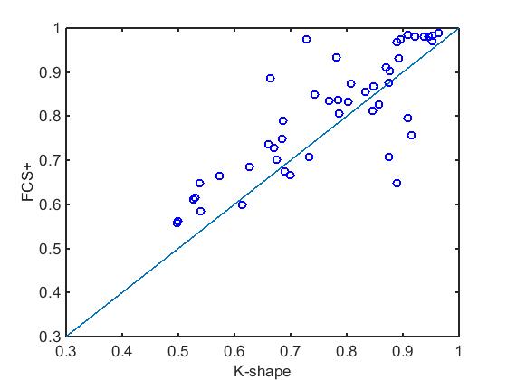
(a) FCS+ vs. k-Shape. Circles above the diagonal indicate datasets for which FCS+ has a better average Rand Index than k-Shape.

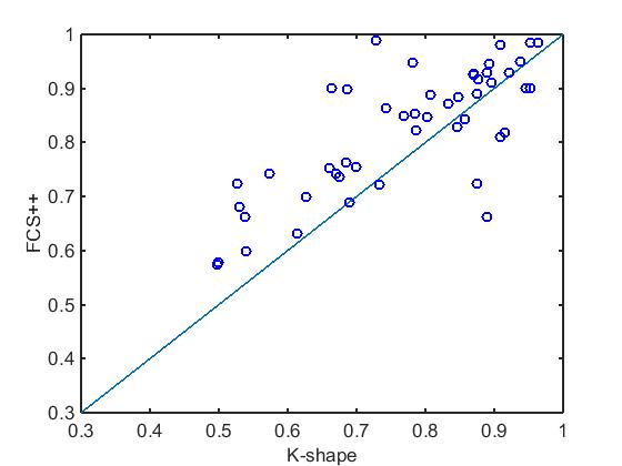
(b) FCS++ vs. k-Shape. Circles above the diagonal indicate datasets for which FCS++ has a better average Rand Index than k-Shape.

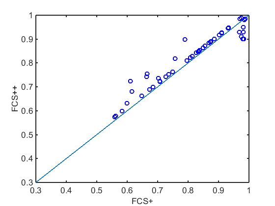
(c) FCS++ vs. FCS+. Circles above the diagonal indicate datasets for which FCS++ has better average Rand Index than FCS+.

Figure 1: Comparisons of k-Shape, FCS+ and FCS++ : average RI values of ten runs over 48 data sets.

VI Numerical Experiments

We use the same 48 synthetic and real data sets that were used in [12]. The 48 sets are all z-normalized, crisply labeled, split into training and test sets, and are collected in the UCR time series database [14]. Our experiments are based on merged versions of the training and test sets. The length of the time series (number of points sampled from the waveforms) in each set is fixed and equal, ranging from $\displaystyle p=24$ to $\displaystyle p=1882$. The number of sample waveforms in the data sets ranges from $\displaystyle n=56$ to $\displaystyle n=9236$. Since all 48 of these data sets are class-labeled, we do not use the external CVIs to select a best candidate from a set of c-partitions at different values of $\displaystyle c$. Here we simply run FCS+ and FCS++ using the specified number of target labels for each of the 48 data sets, acknowledging that the number of labeled classes does not automatically identify the number of clusters that any model and algorithm might think are present in the data. We ran the experiments for each clustering method ten times for each data set. We implemented the clustering methods in MATLAB R2014b (64bits) using the platform: Intel(R) with core(TM)i7 processor and clock speed at 3.60 GHz and 16 GB RAM.
Table I shows the grand averages over $\displaystyle 480$ trials for each of the four crisp external CVIs. Each index was evaluated 10 times for different runs of FCS+ and FCS++ on each of the $\displaystyle 48$ labeled data sets. The ordering for the three algorithms is the same for all four indices. Table I shows that FCS++ is slightly better than FCS+, and in turn, FCS+ outperforms k-Shape by a small margin for all four indices. This demonstrates that the overall quality of both of the new fuzzy methods for clustering waveform data is superior to the k-Shape algorithm in [12].

TABLE I: Grand Average of (480) CVI values
(10 runs per data set x 48 data sets)

CVI	Type	Range	FCS++	FCS+	k-Shape
$\displaystyle\overline{\overline{RI}}$	$\displaystyle(\uparrow)$	$\displaystyle[0,1]$	0.822	0.807	0.772
$\displaystyle\overline{\overline{ARI}}$	$\displaystyle(\uparrow)$	$\displaystyle[-a,1]$	0.461	0.403	0.321
$\displaystyle\overline{\overline{NMI_{M}}}$	$\displaystyle(\uparrow)$	$\displaystyle[0,1]$	0.641	0.534	0.413
$\displaystyle\overline{\overline{VI}}$	$\displaystyle(\downarrow)$	$\displaystyle[0,logn]$	1.010	1.463	2.455

Figure 1 compares each pair of methods graphically. The line through the origin at $\displaystyle 45$ degrees in each view separates $\displaystyle[0,1]\times[0,1]$ into two half-spaces. Each of the views  1(a),  1(b) and  1(c) plots the average values of the Rand Index over $\displaystyle 10$ runs for each of the 48 data sets. The dots represent the $\displaystyle 48$ data sets, and the coordinates of each dot are the average values of the Rand index for the algorithm pair in each view.
For example, the coordinates of points in Figure 1(a) are: horizontal coordinate x = average RI value achieved by $\displaystyle 10$ runs of k-Shape; vertical coordinate y = average RI value achieved by $\displaystyle 10$ runs of FCS+. There are 10 points below the line y = x in Figure  1(a), 1 point on the line, and 37 points above the line. This means that FCS+ achieved a better average result with the RI than k-Shape on 37 of the 48 data sets, they were tied on one data set, and k-Shape had a better average RI than FCS+ on 10 data sets. Figure 1(b) shows that FCS++ is slightly better, with 38 data sets above the line. And Figure 1(c) shows that FCS++ achieves a better result than FCS+ on $\displaystyle 38$ of the $\displaystyle 48$ data sets.
Time complexity analysis: Assume that $\displaystyle n$ and $\displaystyle p$ are the number and the length of the finite time series respectively and $\displaystyle c$ is the number of clusters. All three algorithms use the SBD function to measure dissimilarity between data points and centroids. The SBD function requires $\displaystyle O(plog(p))$ time to calculate this measurement. The implementation of FCM as shown in Algorithm 1 is $\displaystyle O(npc^{2})$. k-Shape uses the k-means algorithm as its underlying clustering algorithm, where the time complexity of k-means is $\displaystyle O(npc)$. Now, the time complexity for the FCS+ algorithm can be calculated as $\displaystyle O(ncplog(p))$ time. In FCS++ and k-Shape clustering algorithms, there is a refinement step, which for every cluster calculates matrix $\displaystyle M$ with $\displaystyle O(p^{2})$ time complexity, and then computes an eigenvalue decomposition on $\displaystyle M$ with $\displaystyle O(p^{3})$ time complexity. Therefore, the complexity of the refinement step is $\displaystyle O(max\{np^{2},cp^{3}\})$. As a result, the per iteration time complexity of FCS++ and k-Shape are $\displaystyle O(max\{nc^{2}plog(p),np^{2},cp^{3}\})$ and $\displaystyle O(max\{ncplog(p),np^{2},cp^{3}\})$ time respectively. Thus, all three algorithms are linear in the number of time series, and the major portion of the computational cost rests with $\displaystyle p$, the length of the time series.
Table II shows the average CPU time taken by each of the three algorithms to evaluate the Rand index for 10 runs of FCM on each of the $\displaystyle 48$ data sets. FCS+ takes roughly $\displaystyle 9.5$ secs per run, whereas the other two required about three times that, FCS++ topping out at about $\displaystyle 25$ secs per run. This is easy to understand: FCS+ does not use SE Algorithm 3, so it is considerably less expensive computationally than the other two algorithms. Overall, these algorithms are reasonable fast for the $\displaystyle 48$ data sets used in our experiments.

TABLE II: Average run time for 480 values of the Rand Index (48 data sets, 10 runs each)

Algorithm	Ave. CPU Time (in seconds)
FCS+	9.51
k-Shape	22.95
FCS++	25.04

TABLE III: Wilcoxon test to compare three clustering methods in terms of accuracy based on $\displaystyle RI$, $\displaystyle ARI$, and $\displaystyle NMI_{M}$ validity method. $\displaystyle R^{+}$ corresponds to the sum of the ranks for the method on the left and $\displaystyle R^{-}$ for the right

	$\displaystyle RI$ Accuracy			$\displaystyle ARI$ Accuracy			$\displaystyle NMI_{M}$ Accuracy
Method	$\displaystyle R^{+}$	$\displaystyle R^{-}$	$\displaystyle\rho$-value	$\displaystyle R^{+}$	$\displaystyle R^{-}$	$\displaystyle\rho$-value	$\displaystyle R^{+}$	$\displaystyle R^{-}$	$\displaystyle\rho$-value
k-Shape vs FCS++	215	913	$\displaystyle 1.304e^{-04}$	66.5	1061.5	$\displaystyle 1.403e^{-07}$	75	1053	$\displaystyle 1.426e^{-07}$
k-Shape vs FCS+	238	813	$\displaystyle 3.309e^{-04}$	154	897	$\displaystyle 6.848e^{-06}$	81	970	$\displaystyle 1.991e^{-07}$
FCS++ vs FCS+	931	245	$\displaystyle 2.608e^{-04}$	1036.5	139.5	$\displaystyle 4.199e^{-06}$	1009	167	$\displaystyle 4.199e^{-05}$

Statistical analysis: We used two statistical tests that assess the statistical significance of the performance of the various methods. First, we perform pairwise comparisons between different methods using the Wilcoxon signed-rank test[64]. The test returns a $\displaystyle\rho$-value associated with each comparison, representing the lowest level of significance of a hypothesis that results in a rejection. This value can be used to determine whether two algorithms have significantly different performance and to what extent. For all the comparisons in this study the significance level $\displaystyle\alpha$ is set to $\displaystyle 0.05$. Table III summarizes these comparisons on all the accuracy results from the three algorithms over 48 datasets. In the three mentioned tables, the $\displaystyle\rho$-value is less than the significance level ($\displaystyle\alpha=0.05$), which means that there is a significant difference between the accuracy of algorithms. To illustrate, consider the RI Accuracy, where the first row compares k-Shape with FCS++. The sum of ranks for k-Shape is less than the sum of ranks for FCS++. Therefore, the accuracy of FCS++ is better than k-Shape clustering. Another statistical test that enables us to compare the three clustering algorithms is Friedman’s test [65]. The Friedman test is a non-parametric statistical test for differences between groups. Figure 2 shows the results of applying Friedman’s test to the three clustering algorithms with respect to the three max optimal CVIs used in our study. Friedman’s test supports the conclusions drawn from Wilcoxon’s test, viz., that FCS++ is superior to FCS+, which is in turn superior to k-Shape.

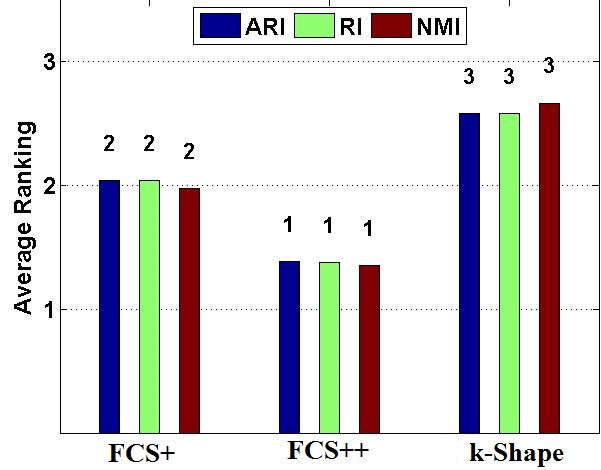
Figure 2: Comparison for rankings of clustering accuracy methods for 3 metrics. The bars represent average rankings based on the Friedman test, and the number on the top of the bars indicates the ranking of the algorithm, from the best (1) to the worst (3) for each given measure. The ranking is determined for all datasets and finally an average is calculated as the mean of all rankings.

VII Discussion

The authors of [12] assert that k-Shape effectively minimizes the classical HCM objective function $\displaystyle J_{1}(U,P;X)$ when $\displaystyle P$ is computed with SE Algorithm 3 and the model norm is replaced by $\displaystyle SBD(x,y)$. However, (i) no theory is given to support their statement about minimization; (ii) Algorithm 2 was not shown to represent an actual metric distance; and (iii) it is not clear whether the distances from Algorithm 2 should properly be interpreted as squared.
The convergence properties of FCM and HCM are well known [66], and the basic theory for both depends on iterate sequences having the descent property, i.e., that for successive iterates, $\displaystyle J_{m}(U_{t+1},V_{t+1})\leq J_{m}(U_{t},V_{t})$. The objective functions that might be optimized by these three heuristic algorithms are all related in principle to the LSE function at Equation (2), i.e.,

$$\displaystyle J_{m}(U,P;X)=\displaystyle\sum_{k=1}^{n}\displaystyle\sum_{i=1}^{c}(u_{ik})^{m}[\Delta(x_{k},p_{i})]^{2}.$$

Table IV lists the components of $\displaystyle J_{m}(U,P;X)$ for each of the three methods tested in this paper, along with the corresponding information for HCM and FCM. In all cases $\displaystyle P$ is a set of $\displaystyle c$ vectors $\displaystyle V\subset\Re^{cp}$. For FCM, HCM and FCS+ they are unconstrained centroids in $\displaystyle p$ space; for k-Shape and FCS++ the $\displaystyle V$’s are found by shape extraction (Algorithm 3).
Do any of the heuristic methods discussed here generate iterative sequences that endow the objective function obtained by replacing $\displaystyle V\subset\Re^{cp}$ and $\displaystyle\Delta(x_{k},p_{i})^{2}$ in Equation (2) with the parameters shown in Table IV with the descent property? The answer is no. The last column $\displaystyle(\downarrow?)$ of Table IV summarizes what is known about the descent property for each of the five methods.
Figure 3 plots presumptive objective functions based on the parameters in Table II for one run of k-Shape, FCS+, and FCS++ on three different data sets. Each view in this figure shows that the objective function for each algorithm is not always monotone decreasing on successive iterates. Consequently, the descent property (and in turn, any convergence theory that requires it) is ruled out by counterexample for all three of these heuristic schemes.

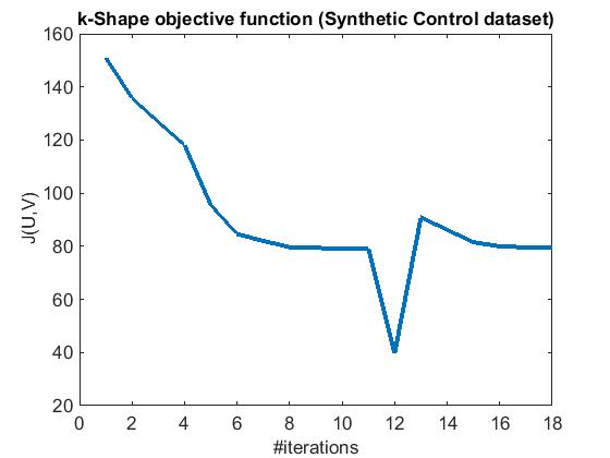
(a) $\displaystyle J(U,V;X)$ for one run of k-Shape: X=Synthetic Control Data

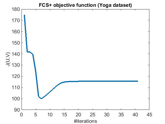
(b) $\displaystyle J(U,V;X)$ for one run of FCS+: X=Yoga Data

(c) $\displaystyle J(U,V;X)$ for one run of FCS++: X=Face (All) Data

Figure 3: Objective functions for algorithms k-Shape, FCS+,and FCS++, are not always monotone decreasing on successive iterates

TABLE IV: Presumptive Objective Function Components

Method	U	$\displaystyle[\Delta(x_{k},p_{i})]^{2}$	P	$\displaystyle\downarrow?$
$\displaystyle FCM(m>1)$	$\displaystyle M_{fcn}$	$\displaystyle\|x-v\|_{A}^{2}$	V	✓
$\displaystyle FCM(m=1)$	$\displaystyle M_{hcn}$	$\displaystyle\|x-v\|_{A}^{2}$	V	✓
$\displaystyle(c-means)$
$\displaystyle k-Shape$	$\displaystyle M_{hcn}$	$\displaystyle SBD(x_{k},p_{i})$	SE V	✗
$\displaystyle FCS+$	$\displaystyle H_{mm}(U)$	$\displaystyle SBD(x_{k},p_{i})$	V	✗
$\displaystyle FCS++$	$\displaystyle H_{mm}(U)$	$\displaystyle SBD(x_{k},p_{i})$	SE V	✗

VIII CONCLUSIONS AND FUTURE REASERCH

Two new fuzzy variants of k-Shape were defined. FCS+ arises by substituting $\displaystyle SBD(x_{k},p_{i})$ for $\displaystyle\parallel x-v\parallel_{A}^{2}$ in FCM. FCS++ is FCS+ with the additional substitution of SE V for the prototypes in FCM. For FSC++, partitioning is adapted to the k-Shape algorithm by hardening the fuzzy partitions produced by FCM at each assignment step. We performed the same experiments with $\displaystyle 48$ labeled waveform data sets that were done using k-Shape in [12], and compared the two fuzzy methods to k-Shape using four crisp external cluster validity indices and two statistical tests of significance. All four indices indicate that FCS++ performs somewhat better than FCS+, and in turn, FCS+ is slightly superior to k-Shape. While our numerical results are encouraging, they are by no means definitive. More experiments are needed with other waveform data, including unlabeled data. Another avenue of pursuit is the theory: is SBD a metric? Is there any convergence theory for k-Shape, FCS+ or FCS++? Figure 3 suggests that the short answer is ”probably not.” Moreover, any satisfactory convergence theory has to overcome the fact that the SBD and SE schemes are computer programs, not functions. Finally, we have not capitalized fully on the fuzzy information available at each assignment step of the two new methods, instead opting to harden $\displaystyle U$ so that $\displaystyle H_{mm}(U)$ can be used directly by Algorithm 3. Surely there is a better use of this information? This is the enterprise we will turn to next.

References

- [1] J. C. Bezdek, Pattern recognition with fuzzy objective function algorithms. Springer Science & Business Media, 2013.
- [2] E. Keogh, “A decade of progress in indexing and mining large time series databases,” in Proceedings of the 32nd international conference on Very large data bases. VLDB Endowment, 2006, pp. 1268–1268.
- [3] E. Keogh and C. A. Ratanamahatana, “Exact indexing of dynamic time warping,” Knowledge and information systems, vol. 7, no. 3, pp. 358–386, 2005.
- [4] E. Keogh and J. Lin, “Clustering of time-series subsequences is meaningless: implications for previous and future research,” Knowledge and information systems, vol. 8, no. 2, pp. 154–177, 2005.
- [5] F. Petitjean, A. Ketterlin, and P. Gançarski, “A global averaging method for dynamic time warping, with applications to clustering,” Pattern Recognition, vol. 44, no. 3, pp. 678–693, 2011.
- [6] W. Meesrikamolkul, V. Niennattrakul, and C. A. Ratanamahatana, “Shape-based clustering for time series data,” in Advances in knowledge discovery and data mining. Springer, 2012, pp. 530–541.
- [7] B. Hu, Y. Chen, and E. J. Keogh, “Time series classification under more realistic assumptions.” in SDM. SIAM, 2013, pp. 578–586.
- [8] C. A. Ratanamahatana and E. Keogh, “Making time-series classification more accurate using learned constraints.” SIAM, 2004.
- [9] M. Halkidi, Y. Batistakis, and M. Vazirgiannis, “On clustering validation techniques,” Journal of intelligent information systems, vol. 17, no. 2, pp. 107–145, 2001.
- [10] V. Niennattrakul and C. A. Ratanamahatana, “Shape averaging under time warping,” in Electrical Engineering/Electronics, Computer, Telecommunications and Information Technology, 2009. ECTI-CON 2009. 6th International Conference on, vol. 2. IEEE, 2009, pp. 626–629.
- [11] J. Yang and J. Leskovec, “Patterns of temporal variation in online media,” in Proceedings of the fourth ACM international conference on Web search and data mining. ACM, 2011, pp. 177–186.
- [12] J. Paparrizos and L. Gravano, “k-shape: Efficient and accurate clustering of time series,” in Proceedings of the 2015 ACM SIGMOD International Conference on Management of Data. ACM, 2015, pp. 1855–1870.
- [13] J. C. Bezdek, “Fuzzy mathematics in pattern classification,” 1973.
- [14] E. Keogh, X. Xi, L. Wei, and C. A. Ratanamahatana, “The ucr time series classification/clustering homepage,” URL= http://www. cs. ucr. edu/eamonn/time series data, 2006.
- [15] H. Ding, G. Trajcevski, P. Scheuermann, X. Wang, and E. Keogh, “Querying and mining of time series data: experimental comparison of representations and distance measures,” Proceedings of the VLDB Endowment, vol. 1, no. 2, pp. 1542–1552, 2008.
- [16] S. Rani and G. Sikka, “Recent techniques of clustering of time series data: a survey,” International Journal of Computer Applications, vol. 52, no. 15, 2012.
- [17] S. Aghabozorgi, A. S. Shirkhorshidi, and T. Y. Wah, “Time-series clustering–a decade review,” Information Systems, vol. 53, pp. 16–38, 2015.
- [18] X. Wang, K. Smith, and R. Hyndman, “Characteristic-based clustering for time series data,” Data mining and knowledge Discovery, vol. 13, no. 3, pp. 335–364, 2006.
- [19] K. Kalpakis, D. Gada, and V. Puttagunta, “Distance measures for effective clustering of arima time-series,” in Data Mining, 2001. ICDM 2001, Proceedings IEEE International Conference on. IEEE, 2001, pp. 273–280.
- [20] R. Agrawal, C. Faloutsos, and A. Swami, “Efficient similarity search in sequence databases,” in International Conference on Foundations of Data Organization and Algorithms. Springer, 1993, pp. 69–84.
- [21] W. G. Aref, M. G. Elfeky, and A. K. Elmagarmid, “Incremental, online, and merge mining of partial periodic patterns in time-series databases,” IEEE Transactions on Knowledge and Data Engineering, vol. 16, no. 3, pp. 332–342, 2004.
- [22] S. Chu, E. J. Keogh, D. M. Hart, M. J. Pazzani et al., “Iterative deepening dynamic time warping for time series.” in SDM. SIAM, 2002, pp. 195–212.
- [23] C. Faloutsos, M. Ranganathan, and Y. Manolopoulos, Fast subsequence matching in time-series databases. ACM, 1994, vol. 23, no. 2.
- [24] X. Golay, S. Kollias, G. Stoll, D. Meier, A. Valavanis, and P. Boesiger, “A new correlation-based fuzzy logic clustering algorithm for fmri,” Magnetic Resonance in Medicine, vol. 40, no. 2, pp. 249–260, 1998.
- [25] M. Vlachos, G. Kollios, and D. Gunopulos, “Discovering similar multidimensional trajectories,” in Data Engineering, 2002. Proceedings. 18th International Conference on. IEEE, 2002, pp. 673–684.
- [26] A. Banerjee and J. Ghosh, “Clickstream clustering using weighted longest common subsequences,” in Proceedings of the web mining workshop at the 1st SIAM conference on data mining, vol. 143. Citeseer, 2001, p. 144.
- [27] L. Chen and R. Ng, “On the marriage of lp-norms and edit distance,” in Proceedings of the Thirtieth international conference on Very large data bases-Volume 30. VLDB Endowment, 2004, pp. 792–803.
- [28] L. J. Latecki, V. Megalooikonomou, Q. Wang, R. Lakaemper, C. A. Ratanamahatana, and E. Keogh, “Elastic partial matching of time series,” in European Conference on Principles of Data Mining and Knowledge Discovery. Springer, 2005, pp. 577–584.
- [29] L. Chen, M. T. Özsu, and V. Oria, “Robust and fast similarity search for moving object trajectories,” in Proceedings of the 2005 ACM SIGMOD international conference on Management of data. ACM, 2005, pp. 491–502.
- [30] M. D. Morse and J. M. Patel, “An efficient and accurate method for evaluating time series similarity,” in Proceedings of the 2007 ACM SIGMOD international conference on Management of data. ACM, 2007, pp. 569–580.
- [31] X. Wang, A. Mueen, H. Ding, G. Trajcevski, P. Scheuermann, and E. Keogh, “Experimental comparison of representation methods and distance measures for time series data,” Data Mining and Knowledge Discovery, vol. 26, no. 2, pp. 275–309, 2013.
- [32] H. Sakoe and S. Chiba, “Dynamic programming algorithm optimization for spoken word recognition,” Acoustics, Speech and Signal Processing, IEEE Transactions on, vol. 26, no. 1, pp. 43–49, 1978.
- [33] L. Kaufman and P. J. Rousseeuw, Finding groups in data: an introduction to cluster analysis. John Wiley & Sons, 2009, vol. 344.
- [34] J. MacQueen et al., “Some methods for classification and analysis of multivariate observations,” in Proceedings of the fifth Berkeley symposium on mathematical statistics and probability, vol. 1, no. 14. Oakland, CA, USA., 1967, pp. 281–297.
- [35] C. S. Möller-Levet, F. Klawonn, K.-H. Cho, and O. Wolkenhauer, “Fuzzy clustering of short time-series and unevenly distributed sampling points,” in Advances in Intelligent Data Analysis V. Springer, 2003, pp. 330–340.
- [36] Q. Song and B. S. Chissom, “Fuzzy time series and its models,” Fuzzy sets and systems, vol. 54, no. 3, pp. 269–277, 1993.
- [37] V. Niennattrakul and C. A. Ratanamahatana, “On clustering multimedia time series data using k-means and dynamic time warping,” in 2007 International Conference on Multimedia and Ubiquitous Engineering (MUE’07). IEEE, 2007, pp. 733–738.
- [38] S. Theodoridis and K. Koutroumbas, “Pattern recognition–fourth edition, 2009.”
- [39] A. K. Jain and R. C. Dubes, Algorithms for clustering data. Prentice-Hall, Inc., 1988.
- [40] R. O. Duda, P. E. Hart et al., Pattern classification and scene analysis. Wiley New York, 1973, vol. 3.
- [41] M. Gavrilov, D. Anguelov, P. Indyk, and R. Motwani, “Mining the stock market (extended abstract): which measure is best?” in Proceedings of the sixth ACM SIGKDD international conference on Knowledge discovery and data mining. ACM, 2000, pp. 487–496.
- [42] R. Honda, S. Wang, T. Kikuchi, and O. Konishi, “Mining of moving objects from time-series images and its application to satellite weather imagery,” Journal of Intelligent Information Systems, vol. 19, no. 1, pp. 79–93, 2002.
- [43] E. J. Ruiz, V. Hristidis, C. Castillo, A. Gionis, and A. Jaimes, “Correlating financial time series with micro-blogging activity,” in Proceedings of the fifth ACM international conference on Web search and data mining. ACM, 2012, pp. 513–522.
- [44] C. Pouzat, O. Mazor, and G. Laurent, “Using noise signature to optimize spike-sorting and to assess neuronal classification quality,” Journal of neuroscience methods, vol. 122, no. 1, pp. 43–57, 2002.
- [45] U. Rutishauser, E. M. Schuman, and A. N. Mamelak, “Online detection and sorting of extracellularly recorded action potentials in human medial temporal lobe recordings, in vivo,” Journal of neuroscience methods, vol. 154, no. 1, pp. 204–224, 2006.
- [46] A. Friedman, M. D. Keselman, L. G. Gibb, and A. M. Graybiel, “A multistage mathematical approach to automated clustering of high-dimensional noisy data,” Proceedings of the National Academy of Sciences, vol. 112, no. 14, pp. 4477–4482, 2015.
- [47] R. Krishnapuram, H. Frigui, and O. Nasraoui, “Fuzzy and possibilistic shell clustering algorithms and their application to boundary detection and surface approximation. i,” Fuzzy Systems, IEEE Transactions on, vol. 3, no. 1, pp. 29–43, 1995.
- [48] R. J. Hathaway and J. C. Bezdek, “Switching regression models and fuzzy clustering,” Fuzzy Systems, IEEE Transactions on, vol. 1, no. 3, pp. 195–204, 1993.
- [49] L. Bobrowski and J. C. Bezdek, “c-means clustering with the l l and l∞ norms,” Systems, Man and Cybernetics, IEEE Transactions on, vol. 21, no. 3, pp. 545–554, 1991.
- [50] S. P. Lloyd, “Least squares quantization in pcm,” Information Theory, IEEE Transactions on, vol. 28, no. 2, pp. 129–137, 1982.
- [51] R. Giusti and G. E. Batista, “An empirical comparison of dissimilarity measures for time series classification,” in Intelligent Systems (BRACIS), 2013 Brazilian Conference on. IEEE, 2013, pp. 82–88.
- [52] F. Petitjean and P. Gançarski, “Summarizing a set of time series by averaging: From steiner sequence to compact multiple alignment,” Theoretical Computer Science, vol. 414, no. 1, pp. 76–91, 2012.
- [53] L. Wang and T. Jiang, “On the complexity of multiple sequence alignment,” Journal of computational biology, vol. 1, no. 4, pp. 337–348, 1994.
- [54] T. A. Runkler and J. C. Bezdek, “Alternating cluster estimation: a new tool for clustering and function approximation,” Fuzzy Systems, IEEE Transactions on, vol. 7, no. 4, pp. 377–393, 1999.
- [55] R. N. Dave and K. Bhaswan, “Adaptive fuzzy c-shells clustering and detection of ellipses,” Neural Networks, IEEE Transactions on, vol. 3, no. 5, pp. 643–662, 1992.
- [56] G. W. Milligan and M. C. Cooper, “An examination of procedures for determining the number of clusters in a data set,” Psychometrika, vol. 50, no. 2, pp. 159–179, 1985.
- [57] D. T. Anderson, J. C. Bezdek, M. Popescu, and J. M. Keller, “Comparing fuzzy, probabilistic, and possibilistic partitions,” Fuzzy Systems, IEEE Transactions on, vol. 18, no. 5, pp. 906–918, 2010.
- [58] Y. Lie, J. C. Bezdek, J. Chan, N. X. Nguyen, S. Romano, and J. Bailey, “Extending information-theoretic validity indices for fuzzy clustering,” in press, Fuzzy Systems, IEEE Transactions on, 2016.
- [59] O. Arbelaitz, I. Gurrutxaga, J. Muguerza, J. M. Pérez, and I. Perona, “An extensive comparative study of cluster validity indices,” Pattern Recognition, vol. 46, no. 1, pp. 243–256, 2013.
- [60] W. M. Rand, “Objective criteria for the evaluation of clustering methods,” Journal of the American Statistical association, vol. 66, no. 336, pp. 846–850, 1971.
- [61] L. Hubert and P. Arabie, “Comparing partitions,” Journal of classification, vol. 2, no. 1, pp. 193–218, 1985.
- [62] M. Meilă, “Comparing clusterings—an information based distance,” Journal of multivariate analysis, vol. 98, no. 5, pp. 873–895, 2007.
- [63] N. X. Vinh, J. Epps, and J. Bailey, “Information theoretic measures for clusterings comparison: Variants, properties, normalization and correction for chance,” The Journal of Machine Learning Research, vol. 11, pp. 2837–2854, 2010.
- [64] F. Wilcoxon, “Individual comparisons by ranking methods,” Biometrics bulletin, vol. 1, no. 6, pp. 80–83, 1945.
- [65] M. Friedman, “The use of ranks to avoid the assumption of normality implicit in the analysis of variance,” Journal of the american statistical association, vol. 32, no. 200, pp. 675–701, 1937.
- [66] J. C. Bezdek, “A convergence theorem for the fuzzy isodata clustering algorithms,” IEEE Transactions on Pattern Analysis & Machine Intelligence, no. 1, pp. 1–8, 1980.