Analyzing Linear Dynamical Systems:
From Modeling to Coding and Learning

Abstract

Encoding time-series with Linear Dynamical Systems (LDSs) leads to rich models with applications ranging from dynamical texture recognition to video segmentation to name a few. In this paper, we propose to represent LDSs with infinite-dimensional subspaces and derive an analytic solution to obtain stable LDSs. We then devise efficient algorithms to perform sparse coding and dictionary learning on the space of infinite-dimensional subspaces. In particular, two solutions are developed to sparsely encode an LDS. In the first method, we map the subspaces into a Reproducing Kernel Hilbert Space (RKHS) and achieve our goal through kernel sparse coding. As for the second solution, we propose to embed the infinite-dimensional subspaces into the space of symmetric matrices and formulate the sparse coding accordingly in the induced space. For dictionary learning, we encode time-series by introducing a novel concept, namely the two-fold LDSs. We then make use of the two-fold LDSs to derive an analytical form for updating atoms of an LDS dictionary, i.e., each atom is an LDS itself. Compared to several baselines and state-of-the-art methods, the proposed methods yield higher accuracies in various classification tasks including video classification and tactile recognition.

Keywords: Linear Dynamical System (LDS), sparse coding, dictionary learning, infinite-dimensional subspace, time-series, two-fold LDS

1 Introduction

This paper introduces techniques to encode and learn from Linear Dynamical Systems (LDSs). Analyzing, classifying and prediction from time-series is an active and multi-disciplinary research area. Examples include financial time-series forecasting Kim (2003), the analysis of video data Afsari et al. (2012) and biomedical data Brunet et al. (2011).

Inference from time-series is not, by any measure, an easy task Afsari and Vidal (2014); Ravichandran et al. (2013). A reasonable and advantageous strategy, from both theoretical and computational points of view, is to simplify the problem by assuming that time-series are generated by models from a specific parametric class. Modeling time-series by LDSs is of one such attempt, especially when facing high-dimensional time-series (e.g. videos). The benefits of modeling with LDSs are twofold: I. the LDS model enables a rich representation, meaning LDSs can approximate a large class of stochastic processes Afsari and Vidal (2014), II. compared to vectorial ARMA models Johansen (1995), LDSs are less prone to the curse of dimensionality. This is an attractive property for vision applications where data is usually high-dimensional.

In the past decade, sparse coding has been successfully exploited in various vision tasks such as image restoration Mairal et al. (2008), face recognition Wright et al. (2009), and texture classification Mairal et al. (2009b) to name a few. In sparse coding, natural signals such as images are represented by a combination of a few basis elements (or atoms of a dictionary). While being extensively studied, little is known on combining sparse coding techniques with LDS modeling to yield robust techniques. In this paper, we generalize sparse coding from Euclidean spaces to the space of LDSs. In particular, we show how an LDS can be reconstructed by a superposition of LDS atoms, while the coefficients of the superposition are enforced to be sparse. We also show how a dictionary of LDS atoms can be learned from data. Sparse coding with the learned LDS dictionary can then be seamlessly used to categorize spatio-temporal data. The importance of our work lies in the fact that to achieve our goals, we need to develop techniques that work with the non-Euclidean space of LDSs Afsari et al. (2012); Ravichandran et al. (2013).

Contributions.

1. Unlike previous attempts that model LDSs with finite-dimensional subspaces, we propose to describe LDSs by infinite-dimensional subspaces. It will be shown that infinite-dimensional modeling not only encodes the full evolution of the sequences but also reduces the computational cost.

2. We propose a simple, yet effective way to stabilize the transition matrix of an LDS. We show that while the stabilization is done in closed-form, the transition matrices maintain sufficient discriminative information to accommodate classification.

3. To perform sparse coding, we propose two techniques that work with infinite-dimensional subspaces. As for the first technique, we map the infinite-dimensional subspaces into a Reproducing Kernel Hilbert Space (RKHS) and formulate the coding problem as a kernel sparse coding problem. In the second approach, we make use of a diffeomorphic mapping to embed the infinite-dimensional subspaces into the space of symmetric matrices and formulate the sparse coding in the induced space.

4. For dictionary learning, we propose to encode the time-series with a novel concept, namely the two-fold LDS. A two-fold LDS can be understood as an structured LDS and enables us to derive an analytical form for updating the dictionary atoms.

Before concluding this part, we would like to highlight that the proposed algorithms outperform state-of-the-art methods on various recognition tasks including video classification and tactile recognition; Figure 1 demonstrates a conceptual diagram of the methods developed in this paper.

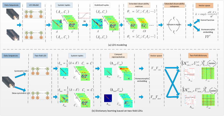
Figure 1: The flowcharts of our LDS modeling formulation and dictionary learning algorithm.

2 Related Work

To analyze LDSs, one should start with a proper geometry. As a result of an invariance property (will be discussed in § 4.3), the space of LDSs is not Euclidean Afsari et al. (2012); Ravichandran et al. (2013). Worse is the fact that the proper geometry, i.e., a structure capturing the invariances imposed by LDSs, is still not fully developed Ravichandran et al. (2013). Nevertheless, various metrics such as Kullback-Leibler divergence Chan and Vasconcelos (2005), Chernoff distance Woolfe and Fitzgibbon (2006), Binet-Cauchy kernel Vishwanathan et al. (2007) and group distance Afsari et al. (2012) have been proposed to measure the distances between LDSs. An alternative solution is to make use of the extended observability subspace to represent an LDS Saisan et al. (2001); Chan and Vasconcelos (2007); Ravichandran et al. (2013); Turaga et al. (2011). Comparing LDSs is then achieved by measuring the subspace angles as applied for example in the Martin distance Martin (2000); De Cock and De Moor (2002).

Recent studies attempt to approximate the extended observability matrix of an LDS by a finite-dimensional subspace Turaga et al. (2011); Harandi et al. (2013, 2015). With such modeling, the geometry of finite-dimensional Grassmannians can be used to analyze LDSs. For example, the geometry of finite-dimensional Grassmannian is used to perform sparse coding and dictionary learning in Harandi et al. (2015) and clustering in Turaga et al. (2011).

One obvious drawback of the aforementioned school of thought and what we avoid in this paper is modeling with finite-dimensional Grassmannians. For example and in the context of dictionary learning, with the finite approximation, only a dictionary of finite observability matrices can be learned. In general, an LDS is identified by its measurement and transition matrices, both are necessary for further analysis (e.g., video registration Ravichandran and Vidal (2011)). To the best of our knowledge, while a finite approximation to the observability matrix can be obtained from the measurement and transition matrices, the reverse action (i.e., obtaining the measurement and transition matrices from the finite observability matrix) is not possible. On the contrary and as we will see later, infinite-dimensional modeling enables us to learn the system parameters of the dictionary explicitly and reduces the computational cost significantly. We draw the reader’s attention to similar observations made in the context of classification (see for example  Saisan et al. (2001); Chan and Vasconcelos (2007); Ravichandran et al. (2013)), hinting that coding and dictionary learning with infinite LDSs can be fruitful.

In our preliminary study Huang et al. (2016b), to learn an LDS dictionary, we assumed that the transition matrices of LDS models are symmetric. Encoding sequences with symmetric LDSs limits the generalization power to some extent. In this work, we extend the methods developed in Huang et al. (2016b) and model sequences via two-fold LDSs. A two-fold LDS enriches the symmetric models Huang et al. (2016b) by having a skew-symmetric part along with the symmetric one. We show that the system parameters of a two-fold LDS can be obtained similar to a conventional LDS, hence richer models can be obtained without incurring heavy computations. Furthermore, by two-fold LDS modeling, we are able to derive efficient algorithms to update an LDS dictionary with two-fold LDS atoms.

3 Notation

Throughout the paper, bold capital letters denote matrices (e.g., ${\boldsymbol{X}}$) and bold lower-case letters denote column vectors (e.g., ${\boldsymbol{x}}$). $\mathbf{I}_{n}$ is the $n\times n$ identity matrix, $\|\cdot\|_{1}$, $\|\cdot\|_{2}$ and $\|\cdot\|_{F}$ denote $\ell_{1}$, $\ell_{2}$ and Frobenius norm, respectively. ${\boldsymbol{X}}^{\mathrm{T}}$ computes the matrix transposition of ${\boldsymbol{X}}$. The Hermitian transpose of a matrix is shown ^∗, i.e., ${\boldsymbol{X}}^{\ast}$; and $\mathop{\rm Tr}\nolimits({\boldsymbol{X}})$ is the trace operator. $[{\boldsymbol{X}}]_{k}$ returns the $k$-th column of a general matrix ${\boldsymbol{X}}$, and returns only the $k$-th diagonal element if ${\boldsymbol{X}}$ is diagonal; $x_{i,j}$ shows the element at $i$-th row and $j$-th column of ${\boldsymbol{X}}$; $x_{i}$ returns the $i$-th element of the vector ${\boldsymbol{x}}$. The symbol $1i$ is the imaginary unit.

4 LDS Modeling

4.1 LDSs

An LDS describes a time series through the following model:

$$\left\{\begin{aligned} &{\boldsymbol{x}}(t+1)&={\boldsymbol{A}}{\boldsymbol{x}}(t)+{\boldsymbol{B}}{\boldsymbol{v}}(t),\\ &{\boldsymbol{y}}(t)&={\boldsymbol{C}}{\boldsymbol{x}}(t)+{\boldsymbol{w}}(t)+\overline{{\boldsymbol{y}}},\end{aligned}\right.$$ (1)

where ${\boldsymbol{X}}=[{\boldsymbol{x}}(1),\cdots,{\boldsymbol{x}}(\tau)]\in\mathbb{R}^{n\times\tau}$ is a sequence of $n$-dimensional hidden state vectors, and ${\boldsymbol{Y}}=[{\boldsymbol{y}}(1),\cdots,{\boldsymbol{y}}(\tau)]\in\mathbb{R}^{m\times\tau}$ is a sequence of $m$-dimensional observed variables. The model is parameterized by $\Theta=\{{\boldsymbol{A}},{\boldsymbol{B}},{\boldsymbol{C}},{\boldsymbol{R}},\overline{{\boldsymbol{y}}}\}$, where ${\boldsymbol{A}}\in\mathbb{R}^{n\times n}$ is the transition matrix; ${\boldsymbol{C}}\in\mathbb{R}^{m\times n}$ is the measurement matrix; ${\boldsymbol{B}}\in\mathbb{R}^{n\times n_{v}}(n_{v}\leq n)$ is the noise transformation matrix; ${\boldsymbol{v}}(t)\sim\mathcal{N}(0,{\boldsymbol{I}}_{n_{v}})$ and ${\boldsymbol{w}}(t)\sim\mathcal{N}(0,{\boldsymbol{R}})$ denote the process and measurement noise components, respectively; $\overline{{\boldsymbol{y}}}\in\mathbb{R}^{m}$ represents the mean of ${\boldsymbol{Y}}$.

Given the observed sequence, several methods Van Overschee and De Moor (1994); Shumway and Stoffer (1982) have been proposed to learn the optimal system parameters, while the method in Doretto et al. (2003) is widely used. This approach first estimates the state sequence by performing PCA on the observations, and then learns the dynamics in the state space via the least square method. We denote the centered observation matrix as ${\boldsymbol{Y}}^{\prime}=[{\boldsymbol{y}}(1)-\overline{{\boldsymbol{y}}},\cdots,{\boldsymbol{y}}(\tau)-\overline{{\boldsymbol{y}}}]$. Factorizing ${\boldsymbol{Y}}^{\prime}$ by Singular Value Decomposition (SVD) yields ${\boldsymbol{Y}}^{\prime}={\boldsymbol{U}}_{Y}{\boldsymbol{S}}_{Y}{\boldsymbol{V}}_{Y}^{\mathrm{T}}$ where ${\boldsymbol{U}}_{Y}\in\mathbb{R}^{m\times n}$, ${\boldsymbol{U}}_{Y}^{\mathrm{T}}{\boldsymbol{U}}_{Y}={\boldsymbol{I}}_{n}$, ${\boldsymbol{S}}_{Y}\in\mathbb{R}^{n\times n}$, ${\boldsymbol{V}}_{Y}\in\mathbb{R}^{n\times\tau}$, and ${\boldsymbol{V}}_{Y}^{\mathrm{T}}{\boldsymbol{V}}_{Y}={\boldsymbol{I}}_{\tau}$. The measurement matrix ${\boldsymbol{C}}$ and the hidden states ${\boldsymbol{X}}$ are then estimated as ${\boldsymbol{U}}_{Y}$ and ${\boldsymbol{S}}_{Y}{\boldsymbol{V}}_{Y}^{\mathrm{T}}$, respectively. The transition matrix ${\boldsymbol{A}}$ is learned by minimizing the state reconstruction error $J^{2}({\boldsymbol{A}})=\|{\boldsymbol{X}}(1)-{\boldsymbol{A}}{\boldsymbol{X}}(0)\|_{F}^{2}$, where ${\boldsymbol{X}}(0)=[{\boldsymbol{x}}(1),\cdots,{\boldsymbol{x}}(\tau-1)]$, ${\boldsymbol{X}}(1)=[{\boldsymbol{x}}(2),\cdots,{\boldsymbol{x}}(\tau)]$. The optimal ${\boldsymbol{A}}$ is given by ${\boldsymbol{A}}={\boldsymbol{X}}(1){\boldsymbol{X}}(0)^{\dagger}$ with ${\dagger}$ denoting the pseudo-inverse of a matrix. Other parameters of LDSs like ${\boldsymbol{B}}$ and ${\boldsymbol{R}}$ can be estimated when ${\boldsymbol{A}}$ and ${\boldsymbol{C}}$ are obtained (see for example Doretto et al. (2003) for details).

4.2 Learning stable LDSs

An LDS is stable if and only if the eigenvalues of its transition matrix are smaller than $1$ Siddiqi et al. (2007). The stability is an important property, because an unstable LDS can cause significant distortion to an input sequence Huang et al. (2016a). Also, we will show later that having stable LDSs is required when it comes to computing the extended observability subspaces. Since the transition matrix ${\boldsymbol{A}}$ leaned by the method discussed in Doretto et al. (2003) is not naturally stable, various methods have been proposed to enforce stability on LDSs Lacy and Bernstein (2002, 2003); Siddiqi et al. (2007); Huang et al. (2016a). All these methods iteratively update the transition matrix by minimizing the state reconstruction error while satisfying the stability constraint. In this paper, however, we devise an analytic and light-weight method to obtain stable LDSs. To be specific, given the transition matrix ${\boldsymbol{A}}$ computed by the method in Doretto et al. (2003), we factorize ${\boldsymbol{A}}$ using SVD as ${\boldsymbol{A}}={\boldsymbol{U}}_{{\boldsymbol{A}}}{\boldsymbol{S}}_{{\boldsymbol{A}}}{\boldsymbol{V}}_{{\boldsymbol{A}}}^{\mathrm{T}}$. Then, we smooth out the diagonal elements of ${\boldsymbol{S}}_{{\boldsymbol{A}}}$ to be within $(-1,1)$ using

$${\boldsymbol{S}}_{{\boldsymbol{A}}}^{\prime} = 2\mathrm{Sig}(a{\boldsymbol{S}}_{{\boldsymbol{A}}})-1.$$ (2)

Here $\mathrm{Sig}(\cdot)$ is the Sigmoid function and $a>0$ is a scale factor. The new transition matrix is ${\boldsymbol{A}}^{\prime}={\boldsymbol{U}}_{{\boldsymbol{A}}}{\boldsymbol{S}}_{{\boldsymbol{A}}}^{\prime}{\boldsymbol{V}}_{{\boldsymbol{A}}}^{\mathrm{T}}$ and is obviously strictly stable. We call this method as Soft-Normalization (SN). Compared to previous methods, SN involves no optimization process, making it scalable to large-scale problems. Besides, due to the saturation property of the Sigmoid function, SN penalizes the singular values that are near or outside the stable bound, without heavily sacrificing the information encoded in the original transition matrix. The effectiveness of SN will be further demonstrated by our experiments in § 9.2.

Figure 2: Illustration of SN on a sequence from the Cambridge dataset Kim and Cipolla (2009). (a) The complex plane displaying the original eigenvalues; (b) The SN function with various scaling values $a$; (c) The distribution of the transition eigenvalues after SN stabilization with $a=2.5$.

4.3 LDS Descriptors

In an LDS, ${\boldsymbol{C}}$ describes the spatial appearance (${\boldsymbol{C}}$ needs to be orthogonal) and ${\boldsymbol{A}}$ represents the dynamics (${\boldsymbol{A}}$ needs to be stable). Therefore, the tuple $({\boldsymbol{A}},{\boldsymbol{C}})$ can be used describe an LDS. A difficulty in analyzing LDSs stems from the fact that the tuple $({\boldsymbol{A}}$,${\boldsymbol{C}})$ does not lie in a vector space Turaga et al. (2011). In particular, for any orthogonal matrix ${\boldsymbol{P}}\in\mathbb{R}^{n\times n}$, $({\boldsymbol{A}},{\boldsymbol{C}})$ is equivalent to $({\boldsymbol{P}}^{\mathrm{T}}{\boldsymbol{A}}{\boldsymbol{P}},{\boldsymbol{CP}})$ as they represent the very same system. To circumvent this difficulty, a family of approaches opts for the extended observability subspace to represent an LDS Saisan et al. (2001); Chan and Vasconcelos (2007); Ravichandran et al. (2013); Turaga et al. (2011). However and to our best of knowledge, the exact form of the extended observability subspace has never been used before. Below, we will derive the exact form of the extended observability subspace in a systematic way.

The Extended Observability Matrix.
Starting from the initial state ${\boldsymbol{x}}(1)$, the expected observation sequence is obtained as

$$[\mathrm{E}[{\boldsymbol{y}}(1)];\mathrm{E}[{\boldsymbol{y}}(2)];\mathrm{E}[{\boldsymbol{y}}(3)];\cdots]=[{\boldsymbol{C}};{\boldsymbol{C}}{\boldsymbol{A}};{\boldsymbol{C}}{\boldsymbol{A}}^{2};\cdots]{\boldsymbol{x}}(1),$$ (3)

where the extended observability matrix is given by ${\boldsymbol{O}}=[{\boldsymbol{C}};{\boldsymbol{C}}{\boldsymbol{A}};{\boldsymbol{C}}{\boldsymbol{A}}^{2};\cdots]\in\mathbb{R}^{\infty\times n}$. It soon becomes clear that the extended observability matrix can encode the (expected) temporal evolution of the LDS till the infinity. Besides, the column space of ${\boldsymbol{O}}$, i.e. the extended observability subspace, is invariant to the choice of the basis of the state space. Such two properties make the extended observability subspaces suitable for describing LDSs. From here onwards, we show the set of extended observability matrices with $n$-dimensional hidden states by $\mathcal{O}(n,\infty)$.

Inner-product between Observability Matrices.
The inner-product between two extended observability matrices ${\boldsymbol{O}}_{1}$ and ${\boldsymbol{O}}_{2}$, i.e., ${\boldsymbol{O}}_{12}={\boldsymbol{O}}_{1}^{\mathrm{T}}{\boldsymbol{O}}_{2}=\sum_{t=0}^{\infty}({\boldsymbol{A}}_{1}^{t})^{\mathrm{T}}{\boldsymbol{C}}_{1}^{\mathrm{T}}{\boldsymbol{C}}_{2}{\boldsymbol{A}}_{2}^{t}$, can be computed by solving the following Lyapunov Equation

$${\boldsymbol{A}}_{1}^{\mathrm{T}}{\boldsymbol{O}}_{12}{\boldsymbol{A}}_{2}-{\boldsymbol{O}}_{12}=-{\boldsymbol{C}}_{1}^{\mathrm{T}}{\boldsymbol{C}}_{2},$$ (4)

whose solution exists and is unique if both ${\boldsymbol{A}}_{1}$ and ${\boldsymbol{A}}_{2}$ are strictly stable De Cock and De Moor (2002).

Extended Observability Matrix with Orthonormal Columns.
To derive the extended observability subspace, we need to orthonormalize ${\boldsymbol{O}}$. In our preliminary study, orthonormalization was done using the Cholesky decomposition Huang et al. (2016b). Different from Huang et al. (2016b), we propose to perform orthonormalization using SVD as we observed that SVD is more flexible than the Cholesky decomposition even when the system is unstable. To this end, we use SVD to factorize ${\boldsymbol{O}}^{\mathrm{T}}{\boldsymbol{O}}={\boldsymbol{U}}_{o}{\boldsymbol{S}}_{o}{\boldsymbol{U}}_{o}^{\mathrm{T}}$. The columns of ${\boldsymbol{V}}={\boldsymbol{O}}{\boldsymbol{L}}^{-\mathrm{T}}$ are orthogonal and span the same subspace as the columns of ${\boldsymbol{O}}$, where the factor matrix ${\boldsymbol{L}}={\boldsymbol{U}}_{o}{\boldsymbol{S}}_{o}^{1/2}$. Thus, ${\boldsymbol{V}}$ is the orthonormal extended observability matrix. We denote the set of the orthogonal extended observability matrices by $\mathcal{V}(n,\infty)$.

Extended Observability Subspaces.
Let $\mathcal{S}(n,\infty)$ be the set of extended observability subspaces. $\mathcal{S}(n,\infty)$ is the quotient space of $\mathcal{V}(n,\infty)$ with the equivalence relation $\sim$ being: for any ${\boldsymbol{V}}_{1},{\boldsymbol{V}}_{2}\in\mathcal{V}(n,\infty)$, ${\boldsymbol{V}}_{1}\sim{\boldsymbol{V}}_{2}$ if and only if $\mathrm{Span}({\boldsymbol{V}}_{1})=\mathrm{Span}({\boldsymbol{V}}_{2})$, where $\mathrm{Span}({\boldsymbol{V}})$ denotes the subspace spanned by the columns of ${\boldsymbol{V}}$. From the definition of $\mathcal{S}(n,\infty)$, one can conclude immediately that $\mathcal{S}(n,\infty)$ is a special case of infinite Grassmannian $\mathcal{G}(n,\infty)$ Ye and Lim (2014) with an extra intrinsic structure due to the stability and orthonormality constraints on ${\boldsymbol{A}}$ and ${\boldsymbol{C}}$, respectively.

A valid distance between subspaces must be a function of their principle angles Ye and Lim (2014). The definition of principle angles for extended observability subspaces have been provided in De Cock and De Moor (2002), where the $n$ principal angles $0\leq\alpha_{1}\leq\alpha_{2}\leq\cdots\leq\alpha_{n}\leq\pi/2$ between two extended observability subspaces $\mathrm{Span}({\boldsymbol{V}}_{1})$ and $\mathrm{Span}({\boldsymbol{V}}_{2})$ are defined recursively by

$$\begin{aligned} &\cos\alpha_{k}&=&\max_{{\boldsymbol{u}}_{k}\in\mathrm{Span}({\boldsymbol{V}}_{1})}\max_{{\boldsymbol{v}}_{k}\in\mathrm{Span}({\boldsymbol{V}}_{2})}{\boldsymbol{u}}_{k}^{\mathrm{T}}{\boldsymbol{v}}_{k}\\ &~{}~{}~{}\mathrm{s.t.}&&{\boldsymbol{u}}_{k}^{\mathrm{T}}{\boldsymbol{u}}_{k}={\boldsymbol{v}}_{k}^{\mathrm{T}}{\boldsymbol{v}}_{k}=1\\ &&&{\boldsymbol{u}}_{k}^{\mathrm{T}}{\boldsymbol{u}}_{j}={\boldsymbol{v}}_{k}^{\mathrm{T}}{\boldsymbol{v}}_{j}=0,j=1,2,\cdots,k-1\end{aligned}$$ (5)

Principal angles can be calculated more efficiently using $\cos\alpha_{k}=s_{k}({\boldsymbol{V}}_{1}^{\mathrm{T}}{\boldsymbol{V}}_{2})$, with $s_{k}(\cdot)$ denoting the $k$-th singular values and ${\boldsymbol{V}}_{1}^{\mathrm{T}}{\boldsymbol{V}}_{2}={\boldsymbol{L}}_{1}^{-1}{\boldsymbol{O}}_{1}^{\mathrm{T}}{\boldsymbol{O}}_{2}{\boldsymbol{L}}_{2}^{\mathrm{-T}}$. Having principal angles at our disposal, various distances between LDSs can be defined. A widely used one is the Martin distance Martin (2000) defined as:

$$d({\boldsymbol{V}}_{1},{\boldsymbol{V}}_{2})=\sqrt{-\log\prod_{k=1}^{n}\cos^{2}\alpha_{k}}.$$ (6)

5 Sparse Coding with LDSs

In this section, we will show how a given LDS can be sparsely coded if an LDS dictionary (i.e., each atom is an LDS) is at our disposal. We recall that the extended observability subspaces are points on an infinite-dimensional Grassmannian. As such, conventional sparse coding techniques designed for vectorial data cannot be used to solve the coding problem. Here, we propose two strategies to perform sparse coding on LDSs. First, we propose a kernel solution by making use of an implicit mapping from the infinite-dimensional Grassmannian to RKHS. In doing so, we design a subspace kernel function which enables us to perform kernel sparse coding Gao et al. (2010) on LDSs. One drawback of the kernel solution is that, the feature map is implicit. This makes learning an LDS dictionary intractable, when the goal is to have explicit atoms. We thus develop another method for sparse coding by embedding the infinite Grassmannian into the space of symmetric matrices by a diffemorphic mapping. We will then show how sparse coding and dictionary learning can be performed in the space defined by the diffemorphic mapping.

5.1 Kernel Sparse Coding

The idea of sparse coding is to approximate a given sample ${\boldsymbol{x}}\in\mathbb{R}^{n}$ with atoms $\{{\boldsymbol{d}}_{j}\in\mathbb{R}^{n}\}_{j=1}^{J}$ of an over-complete dictionary. Moreover, we want the solution to be sparse, meaning that only a few elements of the solution are non-zero. In the Euclidean space, sparse codes can be obtained by solving the following optimization problem

$$\min_{{\boldsymbol{z}}}l({\boldsymbol{z}},{\boldsymbol{d}})=\|{\boldsymbol{x}}-\sum_{j=1}^{J}z_{j}{\boldsymbol{d}}_{j}\|_{2}^{2}+\lambda\|{\boldsymbol{z}}\|_{1},$$ (7)

where $\lambda$ is the sparsity penalty factor.

Directly plugging the extended observability matrices into (7) is obviously not possible. To get around the difficulty of working with points in $\mathcal{S}(n,\infty)$, we propose to implicitly map the subspaces in $\mathcal{S}(n,\infty)$ to an RKHS $\mathcal{H}$. Let us denote the implicit mapping and its associated kernel by $\phi:\mathcal{S}(n,\infty)\rightarrow\mathcal{H}$ and $k(\cdot,\cdot):\mathcal{S}(n,\infty)\times\mathcal{S}(n,\infty)\to\mathbb{R}$ with the property $k({\boldsymbol{X}}_{1},{\boldsymbol{X}}_{2})=\phi({\boldsymbol{X}}_{1})^{T}\phi({\boldsymbol{X}}_{2})$, respectively. This enables us to formulate sparse coding in $\mathcal{H}$ as

$$\min_{{\boldsymbol{z}}}l({\boldsymbol{z}},{\boldsymbol{D}})=\|\phi({\boldsymbol{X}})-\sum_{j=1}^{J}z_{j}\phi({\boldsymbol{D}}_{j})\|_{2}^{2}+\lambda\|{\boldsymbol{z}}\|_{1},$$ (8)

where ${\boldsymbol{X}}\in\mathcal{S}(n,\infty)$ and $\{{\boldsymbol{D}}_{j}\in\mathcal{S}(n,\infty)\}_{j=1}^{J}$ is the LDS dictionary. The problem in (8) can be simplified into Gao et al. (2010)

$$\min_{{\boldsymbol{z}}}l({\boldsymbol{z}},{\boldsymbol{D}})={\boldsymbol{z}}^{\mathrm{T}}{\boldsymbol{K}}_{{\boldsymbol{D}}}{\boldsymbol{z}}-2{\boldsymbol{z}}^{\mathrm{T}}{\boldsymbol{k}}_{{\boldsymbol{XD}}}+\lambda\parallel{\boldsymbol{z}}\parallel_{1},$$ (9)

with ${\boldsymbol{K}}_{{\boldsymbol{D}}}\in\mathbb{R}^{J\times J},{\boldsymbol{K}}_{{\boldsymbol{D}}}(i,j)=k({\boldsymbol{D}}_{i},{\boldsymbol{D}}_{j})$ and ${\boldsymbol{k}}_{{\boldsymbol{XD}}}\in\mathbb{R}^{J},{\boldsymbol{k}}_{{\boldsymbol{XD}}}(j)=k({\boldsymbol{X}},{\boldsymbol{D}}_{j})$. In our experiments, we use the Radial-Basis-Function (RBF) kernel based on Martin distance as

$$k({\boldsymbol{X}}_{1},{\boldsymbol{X}}_{2})=\exp(-\frac{d^{2}({\boldsymbol{X}}_{1},{\boldsymbol{X}}_{2})}{\sigma^{2}}),$$ (10)

where $d({\boldsymbol{X}}_{1},{\boldsymbol{X}}_{2})$ is the Martin distance defined in Eq. (6). Once the kernel values are computed, methods like homotopy-LARS algorithm Donoho and Tsaig (2008) can be used to solve (9). The RBF kernel was also used by Chan et al. Chan and Vasconcelos (2007); however, the positive definiteness of this kernel was neither proven nor discussed. Fortunately, this kernel are always positive definite for the experiments in the paper.

5.2 Sparse Coding by Diffemorphic Embedding

Different form the kernel-based method mentioned in the previous section, we construct an explicit and diffemorphic mapping to facilitate sparse coding. Inspired by the method proposed in Harandi et al. (2015), we embed $\mathcal{S}(n,\infty)$ into the space of symmetric matrices via the mapping $\Pi:\mathcal{S}(n,\infty)\rightarrow\text{Sym}(\infty),\Pi({\boldsymbol{V}})={\boldsymbol{V}}{\boldsymbol{V}}^{\mathrm{T}}$. The metric on Sym($\infty$) is naturally induced by the Frobenius norm: $\|{\boldsymbol{W}}\|_{F}^{2}=\text{Tr}({\boldsymbol{W}}^{\mathrm{T}}{\boldsymbol{W}})$, ${\boldsymbol{W}}\in\text{Sym}(\infty)$. We note that in general the Frobenius norm of a point on $\mathrm{Sym}(\infty)$ is infinite as a result of infinite dimensionality. However, the Frobenius norm of an embedded point $\Pi(\mathcal{S}(n,\infty))$ is guaranteed to be finite. To prove this, we make use of the following theorem.

Theorem 1

Suppose ${\boldsymbol{V}}_{1},{\boldsymbol{V}}_{2},\cdots,{\boldsymbol{V}}_{M}\in\mathcal{S}(n,\infty)$, and $y_{1},y_{2},\cdots,y_{M}\in\mathbb{R}$. Then,

$$\|\sum_{i=1}^{M}y_{i}\Pi({\boldsymbol{V}}_{i})\|_{F}^{2} = \sum_{i,j=1}^{M}y_{i}y_{j}\|{\boldsymbol{V}}_{i}^{\mathrm{T}}{\boldsymbol{V}}_{j}\|_{F}^{2},$$

Proof  The proof is provided in the appendix.  
Based on this Theorem, the following corollary can be drawn:

Corollary 2

For any ${\boldsymbol{V}}_{1},{\boldsymbol{V}}_{2}\in\mathcal{S}(n,\infty)$, we have

$$\|\Pi({\boldsymbol{V}}_{1})-\Pi({\boldsymbol{V}}_{2})\|_{F}^{2} = 2\left(n-\|{\boldsymbol{V}}_{1}^{\mathrm{T}}{\boldsymbol{V}}_{2}\|_{F}^{2}\right).$$

Furthermore, $\|\Pi({\boldsymbol{V}}_{1})-\Pi({\boldsymbol{V}}_{2})\|_{F}^{2}=2\sum_{k=1}^{n}\sin^{2}\alpha_{k}$, where $\{\alpha_{k}\}_{k=1}^{n}$ are subspace angles between ${\boldsymbol{V}}_{1}$ and ${\boldsymbol{V}}_{2}$. This also indicates that $0\leq\|\Pi({\boldsymbol{V}}_{1})-\Pi({\boldsymbol{V}}_{2})\|_{F}^{2}\leq 2n$.

We note that the mapping $\Pi({\boldsymbol{V}})$ is diffeomorphism (a one-to-one, continuous, and differentiable mapping with a continuous and differentiable inverse), meaning that $\mathcal{S}(n,\infty)$ is topologically isomorphic to the embedding $\Pi(\mathcal{S}(n,\infty))$, i.e., $\mathcal{S}(n,\infty)\cong\Pi(\mathcal{S}(n,\infty))$.

With $\Pi(\cdot)$ at our disposal, the sparse coding can be formulated as $\min\limits_{{\boldsymbol{z}}}l({\boldsymbol{z}},{\boldsymbol{D}})$ where,

$$l({\boldsymbol{z}},{\boldsymbol{D}})=\|{\boldsymbol{X}}{\boldsymbol{X}}^{\mathrm{T}}-\sum_{j=1}^{J}z_{j}{\boldsymbol{D}}_{j}{\boldsymbol{D}}_{j}^{\mathrm{T}}\|_{F}^{2}+\lambda\|{\boldsymbol{z}}\|_{1},$$ (11)

Here ${\boldsymbol{X}}\in\mathcal{S}(n,\infty)$, $\{{\boldsymbol{D}}_{j}\in\mathcal{S}(n,\infty)\}_{j=1}^{J}$ is the LDS dictionary, and ${\boldsymbol{z}}=[z_{1};z_{2};\cdots;z_{J}]$ is the vector of sparse codes. We note that by making use of Thm. 1, we can rewrite $l({\boldsymbol{z}},\mathbb{D})$ as

$$l({\boldsymbol{z}},\mathbb{D})={\boldsymbol{z}}^{\mathrm{T}}{\boldsymbol{K}}_{{\boldsymbol{D}}}{\boldsymbol{z}}-2{\boldsymbol{z}}^{\mathrm{T}}{\boldsymbol{k}}_{{\boldsymbol{X}}{\boldsymbol{D}}}+\lambda\parallel{\boldsymbol{z}}\parallel_{1},$$ (12)

where ${\boldsymbol{K}}_{{\boldsymbol{D}}}(i,j)=\parallel{\boldsymbol{D}}_{i}^{\mathrm{T}}{\boldsymbol{D}}_{j}\parallel_{F}^{2}$ and ${\boldsymbol{k}}_{{\boldsymbol{X}}{\boldsymbol{D}}}(j)=\parallel{\boldsymbol{X}}^{\mathrm{T}}{\boldsymbol{D}}_{j}\parallel_{F}^{2}$. This problem is convex as ${\boldsymbol{K}}_{{\boldsymbol{D}}}$ is positive semi-definite.

Interestingly, Eq. (12) has a very similar form to the general kernel sparse coding presented in (9). The difference is that here we explicitly construct the feature mapping, i.e., $\Pi(\mathcal{S}(n,\infty))$. The kernel function $k({\boldsymbol{X}}_{1},{\boldsymbol{X}}_{2})=\|{\boldsymbol{X}}_{1}^{\mathrm{T}}{\boldsymbol{X}}_{2}\|_{F}^{2}$, known as projection kernel Harandi et al. (2014) is well-known for finite-dimensional Grassmannian. We emphasize that this mapping will enable us to devise an algorithm for dictionary learning in § 6.

5.3 Prediction with Labelled Dictionary

Generally speaking, sparse codes obtained by any of the aforementioned methods can be fed into a generic classifier (resp. regressor) for classification (resp. regression) purposes. However, if a labeled dictionary (i.e., a dictionary where each atom comes with a label) is at our disposal, the reconstruction error can be utilized for classification. This is inspired by the Sparse Representation Classifier (SRC) introduced in Wright et al. (2009). Below, we customize SRC for our case of interest, i.e., LDSs. Let us denote all the dictionary atoms belonging to class $c$ by $\{{\boldsymbol{D}}_{k}^{(c)}\}_{k=1}^{J_{c}}$, with $J_{c}$ showing the total number of atoms in class $c$. The reconstruction error of a sample ${\boldsymbol{X}}$ with respect to class $c$ is defined as

$$e_{c}({\boldsymbol{X}}) = \Big{\|}\Pi({\boldsymbol{X}})-\sum_{j=1}^{J_{c}}{\boldsymbol{z}}_{k}^{(c)}\Pi({\boldsymbol{D}}_{k}^{(c)})\Big{\|}_{F}^{2},$$ (13)

where ${\boldsymbol{z}}_{k}^{(c)}$ is the coefficient associated with atom ${\boldsymbol{D}}_{k}^{(c)}$. The label of ${\boldsymbol{X}}$ is then determined by the class that has the minimum reconstruction error, i.e., $y=\arg\min_{c}e_{c}({\boldsymbol{X}})$.

6 Dictionary learning with LDSs

Assume a set of LDS models $\{{\boldsymbol{X}}_{i}\in\mathcal{S}(n,\infty)\}_{i=1}^{N}$ is given. The problem of dictionary learning is to identify a set $\{{\boldsymbol{D}}_{j}\in\mathcal{S}(n,\infty)\}_{j=1}^{J}$ to best reconstruct the observations according to the cost defined in (11). Formally, this can be written as:

$$\min_{{\boldsymbol{Z}},{\boldsymbol{D}}}L({\boldsymbol{Z}},{\boldsymbol{D}})=\sum_{i=1}^{N}l([{\boldsymbol{Z}}]_{i},{\boldsymbol{D}}),$$ (14)

with ${\boldsymbol{Z}}\in\mathbb{R}^{J\times N}$ denoting the coding matrix and $l([{\boldsymbol{Z}}]_{i},{\boldsymbol{D}})$ as in (12). In general, dictionary learning is an involved problem Aharon et al. (2006); Mairal et al. (2009a). The case here is of course as a result of non-Euclidean structure and infinite-dimensionality of the LDS space.

In the following, we first make use of the diffemorphic embedding proposed in § 5.2 to derive a general formulation for the problem of dictionary learning. As it turns out, the general form of dictionary learning is still complicated to work with so we impose further structures to simplify the problem. This leads to the notion of two-fold LDSs and thus a neat and tractable optimization problem for obtaining the LDS dictionary.

6.1 LDS Dictionary: The General Form

A general practice in dictionary learning is to solve the problem alternatively, meaning learning by repeating the following two steps 1) optimizing the codes when the dictionary is fixed and 2) updating the dictionary atoms when the codes are given. The first is indeed the sparse coding problem in (12) which we already know how to solve. As for the second step, we break the minimization problem into $J$ sub-minimization problems by updating each atom independently. To update the r-th atom, ${\boldsymbol{D}}_{r}$, rearranging (14) and keeping the terms that are dependent on ${\boldsymbol{D}}_{r}$ leads to the sub-problem $\min\limits_{{\boldsymbol{D}}_{r}}\Gamma_{r}$ with

$$\Gamma_{r}=\sum_{i=1}^{N}z_{r,i}\sum_{\begin{subarray}{c}j=1,j\neq r\end{subarray}}^{J}\left(z_{j,i}k({\boldsymbol{D}}_{r},{\boldsymbol{D}}_{j})-k({\boldsymbol{D}}_{r},{\boldsymbol{X}}_{i})\right).$$ (15)

Based on the modeling done in § 4.3, each atom ${\boldsymbol{D}}_{r}$ is an infinite subspace and can be parameterized by its transition and measurement matrices, i.e., the tuple $({\boldsymbol{A}}_{r}^{(d)},{\boldsymbol{C}}_{r}^{(d)})$. Our goal is to determine this tuple to identify ${\boldsymbol{D}}_{r}$. Imposing stability and orthonormality constraints on ${\boldsymbol{A}}_{r}^{(d)}$ and ${\boldsymbol{C}}_{r}^{(d)}$, respectively, results in

$$\min_{{\boldsymbol{A}}_{r}^{(d)},{\boldsymbol{C}}_{r}^{(d)}}\Gamma_{r},~{}~{}~{}~{}\mathrm{s.t.}~{}~{}({\boldsymbol{C}}_{r}^{(d)})^{\mathrm{T}}{\boldsymbol{C}}_{r}^{(d)}=\mathbf{I}_{n};~{}|\mu({\boldsymbol{A}}_{r}^{(d)})|<1.$$ (16)

to determine the r-th atom. Here, $\mu({\boldsymbol{A}}_{r}^{(d)})$ denotes the eigenvalue of ${\boldsymbol{A}}_{r}^{(d)}$ with the largest magnitude. Our goal in dictionary learning is to find the optimal tuples of the dictionary atoms.

There are mainly two difficulties in solving (16): 1. As discussed in § 4.3, $({\boldsymbol{A}}_{r}^{(d)},{\boldsymbol{C}}_{r}^{(d)})$ do not lie in an Euclidean space. This is because for any orthogonal ${\boldsymbol{P}}$, $({\boldsymbol{P}}^{\mathrm{T}}{\boldsymbol{A}}_{r}^{(d)}{\boldsymbol{P}},{\boldsymbol{C}}_{r}^{(d)}{\boldsymbol{P}})$ results in the same objective $\Gamma_{r}$ as that of $({\boldsymbol{A}}_{r}^{(d)},{\boldsymbol{C}}_{r}^{(d)})$. 2. As discussed in Huang et al. (2016a), the stability constraint on ${\boldsymbol{A}}_{r}^{(d)}$ makes the feasible region non-convex. Below, we show how the aforementioned difficulties can be addressed.

6.2 Dictionary learning with Two-fold LDSs

To facilitate the optimization in (16), we propose to impose further, yet beneficial structures on the original problem. In particular, we propose to 1. encoding data sequences with two-fold LDSs where the transition matrix is decomposed into symmetric and skew-symmetric parts; and 2. updating symmetric and skew-symmetric dictionaries separately. We will show that with these modifications, not only stable transition matrices can be obtained but also the measurement matrices can be updated in closed-form.

6.2.1 Encoding Sequences with Two-fold LDSs

The two-fold LDS models the input time series with two independent sub-LDSs

$$\left\{\begin{aligned} {\boldsymbol{x}}_{1}(t+1)&={\boldsymbol{A}}_{sym}{\boldsymbol{x}}_{1}(t)+{\boldsymbol{B}}_{1}{\boldsymbol{v}}_{1}(t),\\ {\boldsymbol{y}}(t)&={\boldsymbol{C}}_{1}{\boldsymbol{x}}_{1}(t)+{\boldsymbol{w}}(t)+\overline{{\boldsymbol{y}}},\end{aligned}\right.$$ (17)

$$\left\{\begin{aligned} {\boldsymbol{x}}_{2}(t+1)&={\boldsymbol{A}}_{skew}{\boldsymbol{x}}_{2}(t)+{\boldsymbol{B}}_{2}{\boldsymbol{v}}_{2}(t),\\ {\boldsymbol{y}}(t)&={\boldsymbol{C}}_{2}{\boldsymbol{x}}_{2}(t)+{\boldsymbol{w}}(t)+\overline{{\boldsymbol{y}}},\end{aligned}\right.$$ (18)

where ${\boldsymbol{A}}_{sym}$ and ${\boldsymbol{A}}_{skew}$, as the names imply, are symmetric and skew-symmetric matrices, respectively. Obviously the two-fold LDS encodes a sequence with two decoupled processes, whose transition matrices are constrained to be symmetric and skew-symmetric, respectively. To learn the system tuples for the two-fold LDS, we can apply the method introduced in Doretto et al. (2003) by additionally enforcing the symmetric and skew-symmetric constraints on the transition matrices of the symmetric and skew-symmetric LDSs, respectively. However, this will involve heavy computations. In this paper, we simply choose ${\boldsymbol{C}}_{1}={\boldsymbol{C}}_{2}={\boldsymbol{C}}$, ${\boldsymbol{A}}_{sym}=\frac{1}{2}({\boldsymbol{A}}+{\boldsymbol{A}}^{\mathrm{T}})$ and ${\boldsymbol{A}}_{skew}=\frac{1}{2}({\boldsymbol{A}}-{\boldsymbol{A}}^{\mathrm{T}})$ where ${\boldsymbol{C}}$ and ${\boldsymbol{A}}$ are given by the original LDS defined in Eq. (1). Our experiments show that such solutions still obtain satisfied results. Furthermore, if all ${\boldsymbol{A}}$’s singular-values have the magnitude less than 1 so do those of ${\boldsymbol{A}}_{sym}$ and ${\boldsymbol{A}}_{skew}$. The details are presented in the appendix.

Table 1: The canonical tuples for data and dictionary systems.

Denotation	Definition
$({\boldsymbol{\Lambda}}_{1,i}^{(x)},{\boldsymbol{U}}_{1,i}^{(x)})$	The symmetric canonical tuples of data ${\boldsymbol{X}}_{i}$
$({\boldsymbol{\Lambda}}_{2,i}^{(x)},{\boldsymbol{U}}_{2,i}^{(x)})$	The skew-symmetric canonical tuples of data ${\boldsymbol{X}}_{i}$
$({\boldsymbol{\Lambda}}_{1,j}^{(d)},{\boldsymbol{U}}_{1,j}^{(d)})$	The canonical tuples of symmetric dictionary ${\boldsymbol{D}}_{j}$
$({\boldsymbol{\Lambda}}_{2,j}^{(d)},{\boldsymbol{U}}_{2,j}^{(d)})$	The canonical tuples of skew-symmetric dictionary ${\boldsymbol{D}}_{j}$

Table 2: Intermediate variables for dictionary learning. $({\boldsymbol{\Lambda}}_{j}^{(d)},{\boldsymbol{U}}_{j}^{(d)})$ and $({\boldsymbol{\Lambda}}_{i}^{(x)},{\boldsymbol{U}}_{i}^{(x)})$ denote the canonical tuples of the $j$-th dictionary atoms and the $i$-th data, respectively. They are corresponded to the symmetric parts of two-fold LDSs when updating symmetric dictionary and skew-symmetric parts when updating skew-symmetric dictionary.

Denotation	Definition
${\boldsymbol{E}}(\lambda,{\boldsymbol{\Lambda}})$	${\boldsymbol{E}}(\lambda,{\boldsymbol{\Lambda}})=\mathrm{diag}([\frac{(1-|\lambda|^{2})(1-|\lambda_{1}|^{2})}{|1-\lambda\lambda_{1}^{*}|^{2}},\cdots,$ $\frac{(1-|\lambda|^{2})(1-|\lambda_{n}|^{2})}{|1-\lambda\lambda_{n}^{*}|^{2}}])$ and $\lambda_{k}=[{\boldsymbol{\Lambda}}]_{k}$
${\boldsymbol{F}}_{r,j,k}$	${\boldsymbol{F}}_{r,j,k}={\boldsymbol{U}}_{j}^{(d)}{\boldsymbol{E}}([{\boldsymbol{\Lambda}}_{r}^{(d)}]_{k},{\boldsymbol{\Lambda}}_{j}^{(d)})({\boldsymbol{U}}_{j}^{(d)})^{*}$
${\boldsymbol{F^{\prime}}}_{r,i,k}$	${\boldsymbol{F^{\prime}}}_{r,i,k}={\boldsymbol{U}}_{i}^{(x)}{\boldsymbol{E}}([{\boldsymbol{\Lambda}}_{r}^{(d)}]_{k},{\boldsymbol{\Lambda}}_{i}^{(x)})({\boldsymbol{U}}_{i}^{(x)})^{*}$
$k({\boldsymbol{D}}_{r},{\boldsymbol{D}}_{j})$	$k({\boldsymbol{D}}_{r},{\boldsymbol{D}}_{j})=\sum_{k=1}^{n}[{\boldsymbol{U}}_{r}^{(d)}]_{k}^{*}{\boldsymbol{F}}_{r,j,k}[{\boldsymbol{U}}_{r}^{(d)}]_{k}$
$k({\boldsymbol{D}}_{r},{\boldsymbol{X}}_{i})$	$k({\boldsymbol{D}}_{r},{\boldsymbol{X}}_{i})=\sum_{k=1}^{n}[{\boldsymbol{U}}_{r}^{(d)}]_{k}^{*}{\boldsymbol{F^{\prime}}}_{r,i,k}[{\boldsymbol{U}}_{r}^{(d)}]_{k}$
${\boldsymbol{S}}_{r,k}$	${\boldsymbol{S}}_{r,k}=\sum_{i=1}^{N}z_{r,i}(\sum_{j=1,j\neq r}^{J}z_{j,i}{\boldsymbol{F}}_{r,j,k}-{\boldsymbol{F^{\prime}}}_{r,i,k})$

6.2.2 Learning a Two-fold Dictionary

Assuming that the dictionary atoms are also generated by two-fold LDSs, we define the reconstruction error over a set of data two-fold LDSs described by $\{{\boldsymbol{X}}_{i}\}_{i=1}^{N}$ as

$$L({\boldsymbol{Z}},{\boldsymbol{D}}_{1,\cdot},{\boldsymbol{D}}_{2,\cdot})\coloneqq$$ (19)

$$\sum_{i=1}^{N}\Big{\|}\Pi({\boldsymbol{X}}_{1,i})-\sum_{j=1}^{J}z_{j,i}^{(1)}\Pi({\boldsymbol{D}}_{1,j})\Big{\|}_{F}^{2}+\|\Pi({\boldsymbol{X}}_{2,i})-\sum_{j=1}^{J}z_{j,i}^{(2)}\Pi({\boldsymbol{D}}_{2,j})\Big{\|}_{F}^{2}.$$

Here, ${\boldsymbol{X}}_{1,i}$ and ${\boldsymbol{X}}_{2,i}$ are respectively the symmetric and skew-symmetric parts of data ${\boldsymbol{X}}_{i}$; ${\boldsymbol{D}}_{1,j}$ and ${\boldsymbol{D}}_{2,j}$ are respectively the symmetric and skew-symmetric parts of the dictionary atom ${\boldsymbol{D}}_{j}$. Note that the codes for ${\boldsymbol{D}}_{1,j}$ and ${\boldsymbol{D}}_{2,j}$ are not necessary equal to each other so as to improve the modeling flexibility. For simplicity, we concatenate the codes for the symmetric and skew-symmetric dictionary atoms into one single code matrix as ${\boldsymbol{Z}}=[{\boldsymbol{z}}_{\cdot,1}^{(1)};\cdots;{\boldsymbol{z}}_{\cdot,N}^{(1)};{\boldsymbol{z}}_{\cdot,1}^{(2)};\cdots;{\boldsymbol{z}}_{\cdot,N}^{(2)}]$. As discussed in § 6.1, Problem (19) can be solved by alternatively updating the codes and dictionary atoms. Given the codes, the dictionary atoms can be learned one by one, leading to the sub-problem given by (15) and (16). To address the sub-problem, we make use of the following lemma (see the appendix for the proof).

Lemma 3

For a symmetric or skew-symmetric transition matrix ${\boldsymbol{A}}$, the system tuple $({\boldsymbol{A}},{\boldsymbol{C}})\in\mathbb{R}^{n\times n}\times\mathbb{R}^{m\times n}$ has the canonical form $({\boldsymbol{\Lambda}},{\boldsymbol{U}})\in\mathbb{R}^{n}\times\mathbb{R}^{m\times n}$, where ${\boldsymbol{\Lambda}}$ is diagonal and ${\boldsymbol{U}}$ is unitary, i.e. ${\boldsymbol{U}}^{\ast}{\boldsymbol{U}}=\mathbf{I}$. Moreover, both ${\boldsymbol{\Lambda}}$ and ${\boldsymbol{U}}$ are real if ${\boldsymbol{A}}$ is symmetric and complex if ${\boldsymbol{A}}$ is skew-symmetric. For the skew-symmetric ${\boldsymbol{A}}$, $({\boldsymbol{\Lambda}},{\boldsymbol{U}})$ is parameterized by a real matrix-pair $({\boldsymbol{\Theta}},{\boldsymbol{Q}})\in\mathbb{R}^{n/2}\times\mathbb{R}^{m\times n}$ where ${\boldsymbol{\Theta}}$ is diagonal, ${\boldsymbol{Q}}$ is orthogonal, and $n$ is even.

For the sake of convenience, we denote the canonical tuples for data and dictionary as in Table 1. We denote the system tuple of ${\boldsymbol{D}}_{j}$ by $({\boldsymbol{\Lambda}}_{j}^{(d)},{\boldsymbol{U}}_{j}^{(d)})$ if specifying the symmetric or skew-symmetric part is not required.

In the conventional LDS modeling, the exact form of the kernel functions in Eq. (15) cannot be obtained due to the implicit calculation of the Lyapunov equation. In contrast, the extra structure imposed on the transition matrices enables us to compute the inner-products between observability matrices and derive the kernel values as required by Eq. (15). In Table 2, we provide the form of $k({\boldsymbol{D}}_{r},{\boldsymbol{D}}_{j})$ and $k({\boldsymbol{D}}_{r},{\boldsymbol{X}}_{i})$ along ${\boldsymbol{E}}(\lambda,{\boldsymbol{\Lambda}}_{j})$, ${\boldsymbol{F}}_{r,j,k}$, ${\boldsymbol{F}}_{r,i,k}^{(1)}$ and ${\boldsymbol{F}}_{r,i,k}^{(2)}$ which are required for computing the kernel functions (see the appendix for the details).

With the kernel functions at our disposal, we make use of the following theorem to recast Eq. (16) into a form that suits our purpose better.

Theorem 4

For the two-fold LDS modeling defined in Eq. (17) and Eq. (18), the sup-problem in Eq. (16) is equivalent to

$$\begin{aligned} &\min_{{\boldsymbol{U}}_{r}^{(d)},{\boldsymbol{\Lambda}}_{r}^{(d)}}&&\sum_{k=1}^{n}[{\boldsymbol{U}}_{r}^{(d)}]_{k}^{*}{\boldsymbol{S}}_{r,k}[{\boldsymbol{U}}_{r}^{(d)}]_{k}\\ &~{}~{}~{}\mathrm{s.t.}&&({\boldsymbol{U}}_{r}^{(d)})^{*}{\boldsymbol{U}}_{r}^{(d)}=\mathbf{I}_{n};\\ &&&-1<[{\boldsymbol{\Lambda}}_{r}^{(d)}]_{k}<1,~{}1\leq k\leq n.\end{aligned}$$ (20)

Here, the matrix ${\boldsymbol{S}}_{r,k}$ (see Table 2) is not dependent on the measurement matrix ${\boldsymbol{U}}_{r}^{(d)}$.

Updating the Symmetric Dictionary

For a symmetric dictionary atom $({\boldsymbol{\Lambda}}_{1,r}^{(d)},{\boldsymbol{U}}_{1,r}^{(d)})$, both ${\boldsymbol{\Lambda}}_{1,r}^{(d)}$ and ${\boldsymbol{U}}_{1,r}^{(d)}$ are real matrices. The matrix ${\boldsymbol{S}}_{r,k}$ in (20) is also guaranteed to be real and symmetric. We further break the optimization in (20) into $n$ sub-minimization problems. That is, to find the optimal pair $([{\boldsymbol{\Lambda}}_{1,r}^{(d)}]_{k},[{\boldsymbol{U}}_{1,r}^{(d)}]_{k})$, we fix all the other pairs $\{[{\boldsymbol{\Lambda}}_{1,r}^{(d)}]_{o},[{\boldsymbol{U}}_{1,r}^{(d)}]_{o})\}_{o=1,o\neq k}^{n}$. As such, we need to optimize the following sub-problem,

$$\begin{aligned} &\min_{[{\boldsymbol{U}}_{1,r}^{(d)}]_{k},[{\boldsymbol{\Lambda}}_{1,r}^{(d)}]_{k}}&&[{\boldsymbol{U}}_{1,r}^{(d)}]_{k}^{\mathrm{T}}{\boldsymbol{S}}_{r,k}[{\boldsymbol{U}}_{1,r}^{(d)}]_{k}\\ &~{}~{}~{}~{}~{}~{}\mathrm{s.t.}&&({\boldsymbol{U}}_{1,r}^{(d)})^{\mathrm{T}}{\boldsymbol{U}}_{1,r}^{(d)}=\mathbf{I}_{n},\\ &&&-1<[{\boldsymbol{\Lambda}}_{1,r}^{(d)}]_{k}<1.\end{aligned}$$ (21)

The optimal $[{\boldsymbol{U}}_{1,r}^{(d)}]_{k}$ is obtained by the following theorem.

Theorem 5

Let $[{\boldsymbol{U}}_{1,r}^{(d)}]_{-k}\in\mathbb{R}^{m\times(n-1)}$ denote the sub-matrix obtained from ${\boldsymbol{U}}_{1,r}^{(d)}$ by removing the $k$-th column, i.e.,

$$[{\boldsymbol{U}}_{1,r}^{(d)}]_{-k}=\Big{(}[{\boldsymbol{U}}_{1,r}^{(d)}]_{1};\cdots;[{\boldsymbol{U}}_{1,r}^{(d)}]_{k-1};[{\boldsymbol{U}}_{1,r}^{(d)}]_{k+1};\cdots;[{\boldsymbol{U}}_{1,r}^{(d)}]_{n}\Big{)}.$$

Define ${\boldsymbol{W}}=[{\boldsymbol{w}}_{1},\cdots,{\boldsymbol{w}}_{m-n+1}]\in\mathbb{R}^{m\times(m-n+1)}$ as the orthogonal complement basis of $[{\boldsymbol{U}}_{1,r}^{(d)}]_{-k}$. If ${\boldsymbol{u}}\in\mathbb{R}^{(m-n+1)}$ is the eigenvector of ${\boldsymbol{W}}^{\mathrm{T}}{\boldsymbol{S}}_{r,k}{\boldsymbol{W}}$ corresponding to the smallest eigenvalue, then ${\boldsymbol{W}}{\boldsymbol{u}}$ is the optimal solution of $[{\boldsymbol{U}}_{1,r}^{(d)}]_{-k}$ for Eq. (21).

Proof  See the appendix for the proof of this theorem.  
In terms of the transition term $[{\boldsymbol{\Lambda}}_{1,r}^{(d)}]_{k}$, solving (21) is actually to solve a minimization problem with bound constraints. Here, we transform (21) to an unconstrained problem using an auxiliary variable $\rho$ satisfying

$$[{\boldsymbol{\Lambda}}_{1,r}^{(d)}]_{k}=2\mathrm{Sig}(a\rho)-1.$$ (22)

This is indeed similar to the SN stabilization method introduced in § 4.2. With this trick $[{\boldsymbol{\Lambda}}_{1,r}^{(d)}]_{k}$ is naturally bounded in $(-1,1)$, hence enabling us to apply gradient-descent methods to update $[{\boldsymbol{\Lambda}}_{1,r}^{(d)}]_{k}$. More specifically, let $\Phi(r,k)=[{\boldsymbol{U}}_{1,r}^{(d)}]_{k}^{\mathrm{T}}{\boldsymbol{S}}_{r,k}[{\boldsymbol{U}}_{1,r}^{(d)}]_{k}$. Then,

$$\frac{\partial\Phi(r,k)}{\partial\rho}=2\frac{\partial\Phi(r,k)}{\partial[{\boldsymbol{\Lambda}}_{1,r}^{(d)}]_{k}}\frac{\partial[{\boldsymbol{\Lambda}}_{1,r}^{(d)}]_{k}}{\partial\rho}\;.$$

In practice, We first update $\rho$ with its gradient, and then return back to $[{\boldsymbol{\Lambda}}_{1,r}^{(d)}]_{k}$ via Eq. (22).

Updating the Skew-symmetric Dictionary

For a skew-symmetric atom $({\boldsymbol{\Lambda}}_{2,r}^{(d)},{\boldsymbol{U}}_{2,r}^{(d)})$, both ${\boldsymbol{\Lambda}}_{2,r}^{(d)}$ and ${\boldsymbol{U}}_{2,r}^{(d)}$ are complex matrices. As such, Theorem 5 and Eq.(22) cannot be directly used to update the dictionary. However, since $({\boldsymbol{\Lambda}}_{2,r}^{(d)},{\boldsymbol{U}}_{2,r}^{(d)})$ can be parametrized by a real tuple $({\boldsymbol{\Theta}},{\boldsymbol{Q}})$, a similar approach to that of symmetric dictionary can be utilized for updates. More specifically, fixing the contribution of all the other pairs, to update the pairs $([{\boldsymbol{\Theta}}]_{k},[{\boldsymbol{Q}}]_{2k-1})$ and $([{\boldsymbol{\Theta}}]_{k},[{\boldsymbol{Q}}]_{2k})$, we need to solve

$$\begin{aligned} &\min_{\begin{subarray}{c}[{\boldsymbol{Q}}]_{2k-1:2k}\\ [{\boldsymbol{\Theta}}]_{k}\end{subarray}}&&[{\boldsymbol{Q}}]_{2k-1}^{\mathrm{T}}{\boldsymbol{S^{\prime}}}_{r,k}[{\boldsymbol{Q}}]_{2k-1}+[{\boldsymbol{Q}}]_{2k}^{\mathrm{T}}{\boldsymbol{S^{\prime}}}_{r,k}[{\boldsymbol{Q}}]_{2k}+\delta_{r,k}\\ &~{}~{}~{}~{}~{}~{}\mathrm{s.t.}&&{\boldsymbol{Q}}^{\mathrm{T}}{\boldsymbol{Q}}=\mathbf{I}_{n},\\ &&&-1<[{\boldsymbol{\Theta}}]_{k}<1.\end{aligned}$$ (23)

Here, ${\boldsymbol{S^{\prime}}}_{r,k}=\frac{1}{2}({\boldsymbol{S}}_{r,2k-1}+{\boldsymbol{S}}_{r,2k})$ is a real symmetric matrix. As shown in the appendix, $\delta_{r,k}$ is small and can be neglected in practice. As such, the optimal $[{\boldsymbol{Q}}]_{2k-1}$ and $[{\boldsymbol{Q}}]_{2k}$ are given by the following theorem.

Theorem 6

Let $[{\boldsymbol{Q}}]_{-2}\in\mathbb{R}^{m\times(n-2)}$ be a sub-matrix of ${\boldsymbol{Q}}$ obtained by removing the $(2k-1)$-th and $2k$-th columns, i.e.,

$$[{\boldsymbol{Q}}]_{-2}=\Big{(}[{\boldsymbol{Q}}]_{1};\cdots;[{\boldsymbol{Q}}]_{2k-2};[{\boldsymbol{Q}}]_{2k+1};\cdots;[{\boldsymbol{Q}}]_{n}\Big{)}.$$

Define ${\boldsymbol{W}}=[{\boldsymbol{w}}_{1},\cdots,{\boldsymbol{w}}_{m-n+2}]\in\mathbb{R}^{m\times(m-n+2)}$ as the orthogonal complement basis of $[{\boldsymbol{Q}}]_{-2}$. If ${\boldsymbol{u}}_{1},{\boldsymbol{u}}_{2}\in\mathbb{R}^{(m-n+1)}$ are the eigenvectors of ${\boldsymbol{W}}^{\mathrm{T}}{\boldsymbol{S^{\prime}}}_{r,k}{\boldsymbol{W}}$ corresponding to the smallest two eigenvalues, then ${\boldsymbol{W}}{\boldsymbol{u}}_{1}$ and ${\boldsymbol{W}}{\boldsymbol{u}}_{2}$ are the solutions of $[{\boldsymbol{Q}}]_{2k-1}$ and $[{\boldsymbol{Q}}]_{2k}$ in Eq. (23), respectively.

Proof  See the appendix for the proof of this theorem.  
To update ${\boldsymbol{\Theta}}_{r}$, we also apply the gradient-based method by first smoothing out its value using

$$[{\boldsymbol{\Theta}}]_{k}=2\mathrm{Sig}(a\rho)-1,$$ (24)

and then passing the gradient of the objective with respect to $\rho$. Once $([{\boldsymbol{\Theta}}]_{k},[{\boldsymbol{Q}}]_{2k-1})$ are updated, the dictionary atom $({\boldsymbol{\Lambda}}_{2,r}^{(d)},{\boldsymbol{U}}_{2,r}^{(d)})$ can be obtained from Lemma 3. All the aforementioned details are summarized in Algorithm 1.

Algorithm 1 Dictionary learning with LDSs

  Input: ${\boldsymbol{X}}$

  Extract the system parameters of the data sequences by the two-fold LDS: ${\boldsymbol{C}}_{1}={\boldsymbol{C}}_{2}={\boldsymbol{C}},{\boldsymbol{A}}_{sym}=\frac{1}{2}({\boldsymbol{A}}+{\boldsymbol{A}}^{\mathrm{T}}),{\boldsymbol{A}}_{skew}=\frac{1}{2}({\boldsymbol{A}}-{\boldsymbol{A}}^{\mathrm{T}})$;

  Initialize the symmetric and skew-symmetric dictionary atoms by random;

  for $t=1$ to $MaxNumIters$ do

     Learn the sparse codes ${\boldsymbol{Z}}$ by solving Eq. (12), where the kernels are computed as shown in Table 2;

     for $r=1$ to $J$ do

        % update the symmetric dictionary

        for $k=1$ to $n$ do

           Compute ${\boldsymbol{S}}_{r,k}$ as defined in Eq. (20);

           Update $[{\boldsymbol{U}}_{1,r}^{(d)}]_{k}$ according to Theorem 5;

           Update $[{\boldsymbol{\Lambda}}_{1,r}^{(d)}]_{k}$ according to Eq. (22);

        end for

        % update the skew-symmetric dictionary

        for $k=1$ to $\frac{n}{2}$ do

           Compute ${\boldsymbol{S^{\prime}}}_{r,k}$ as defined in Eq. (23);

           Update $[{\boldsymbol{Q}}]_{2k-1:2k}$ according to Theorem 6;

           Update $[{\boldsymbol{\Theta}}]_{k}$ according to Eq. (24);

           Compute $[{\boldsymbol{U}}_{2,r}^{(d)}]_{2k-1:2k}$ via Lemma 3;

           Compute $[{\boldsymbol{\Lambda}}_{2,r}^{(d)}]_{2k-1:2k}$via Lemma 3;

        end for

     end for

  end for

7 Models Considering State Covariances

In our preliminary study Huang et al. (2016b), we incorporate the state covariance matrix ${\boldsymbol{B}}$ into kernel functions as the symmetric structure on the transition matrices might be restrictive in certain cases. Generally speaking and compared to conventional LDSs, the two-fold LDS can model a time-series better. However, we observe that adding the state covariance matrix ${\boldsymbol{B}}$ can boost the performances further (see Fig. 12 for empirical evaluations).

From Eq. (1), the conditional probability of ${\boldsymbol{y}}_{t+1}$ given ${\boldsymbol{x}}(t)$ is $p({\boldsymbol{y}}(t+1)\mid{\boldsymbol{x}}(t))=\mathcal{N}({\boldsymbol{y}}(t+1);{\boldsymbol{CA}}{\boldsymbol{x}}(t)+{\boldsymbol{\bar{y}}},{\boldsymbol{CB}}{\boldsymbol{B}}^{\mathrm{T}}{\boldsymbol{C}}^{\mathrm{T}}+{\boldsymbol{R}})$. Since, the covariance of the state dynamic is our main concern, we assume ${\boldsymbol{R}}\simeq{\boldsymbol{0}}$. Empirically, we observe that stable performances can be attained if ${\boldsymbol{B}}$ is orthogonalized. This can be done by first factorizing ${\boldsymbol{B}}$ using SVD as ${\boldsymbol{B}}={\boldsymbol{U}}_{B}{\boldsymbol{S}}_{B}{\boldsymbol{V}}_{B}^{\mathrm{T}}$, followed by orthogonalizing in the form ${\boldsymbol{B}}={\boldsymbol{B}}{\boldsymbol{U}}_{B}{\boldsymbol{S}}_{B}^{-1/2}$. We define a hybrid kernel function by making use of the covariance term as

$$k({\boldsymbol{X}}_{1},{\boldsymbol{X}}_{2})=\beta k_{m}({\boldsymbol{X}}_{1},{\boldsymbol{X}}_{2})+(1-\beta)k_{cov}({\boldsymbol{X}}_{1},{\boldsymbol{X}}_{2}).$$ (25)

Here, $k_{m}({\boldsymbol{X}}_{1},{\boldsymbol{X}}_{2})$ is the kernel for the extended observability subspaces defined in Eq. (12), $k_{cov}({\boldsymbol{X}}_{1},{\boldsymbol{X}}_{2})=\|{\boldsymbol{H}}_{1}^{\mathrm{T}}{\boldsymbol{H}}_{2}\|_{F}^{2}$ is the kernel value between covariances with ${\boldsymbol{H}}={\boldsymbol{CB}}^{\prime}\in\mathcal{R}^{m\times n_{v}}$ being an orthogonal matrix , and $\beta$ is a weight to trade-off between $k_{m}({\boldsymbol{X}}_{1},{\boldsymbol{X}}_{2})$ and $k_{cov}({\boldsymbol{X}}_{1},{\boldsymbol{X}}_{2})$.

Replacing the kernel function in Eq. (15) with the hybrid kernel in Eq. (25) does not change the algorithm described in Alg. 1 dramatically. The only additional calculation is the update of the covariance term ${\boldsymbol{H}}_{r}^{(d)}$ for the $r$-th atom. We can derive that, when the covariances of other atoms are given. That is to obtain ${\boldsymbol{H}}_{r}^{(d)}$, we can minimize $\mathrm{Tr}(({\boldsymbol{H}}_{r}^{(d)})^{\mathrm{T}}{\boldsymbol{S}}_{cov,r}{\boldsymbol{H}}_{r}^{(d)})$, where ${\boldsymbol{S}}_{cov,r}=\sum_{i=1}^{N}z_{r,i}\sum_{j=1,j\neq r}^{J}(z_{j,i}{\boldsymbol{H}}_{j}^{(d)}({\boldsymbol{H}}_{j}^{(d)})^{\mathrm{T}}-{\boldsymbol{H}}_{i}^{(x)}({\boldsymbol{H}}_{i}^{(x)})^{\mathrm{T}})$. The optimal ${\boldsymbol{H}}_{r}^{(d)}$ is obtained as the eigenvectors of ${\boldsymbol{S}}_{cov,r}$ corresponding to the smallest $n_{v}$ eigenvalues.

8 Computational Complexity

For sparse coding (Eq. (12)), computing the kernel-values is required. In doing so, we need to I) perform the SVD decomposition, II) solve the Lyapunov equation and III) calculate the matrix multiplication, with the complexity of $O(n^{3})$, $O(n^{3})$ and $O(mn^{2})$, respectively. Since usually $n\ll m$, all these computations cost $O(mn^{2})$. Thus computing ${\boldsymbol{K}}_{{\boldsymbol{D}}}$ and ${\boldsymbol{k}}_{{\boldsymbol{DX}}}$ costs $O((NJ+J^{2})mn^{2})$.

As shown in Algorithm 1, for each dictionary atom, we need to calculate ${\boldsymbol{S}}_{r,k}$ and ${\boldsymbol{U}}_{1,r}^{(d)}$ to update the symmetric dictionary and ${\boldsymbol{S}}^{\prime}_{r,k}$ and ${\boldsymbol{U}}_{2,r}^{(d)}$ to update the skew-symmetric dictionary. Computing ${\boldsymbol{S}}_{r,k}$ and ${\boldsymbol{S^{\prime}}}_{r,k}$ requires $O(2J(N+nm^{2})+\gamma nm^{2})$ flops, where $\gamma$ denotes the number of non-zero elements in the $r$-th row of ${\boldsymbol{Z}}$. We apply the Grassmannian-based Conjugate Gradient Method Edelman et al. (1998) to find the smallest eigenvector of ${\boldsymbol{W}}^{\mathrm{T}}{\boldsymbol{S}}_{r,k}{\boldsymbol{W}}$, which has a computational cost of $O(m^{2})$. This operation needs to be repeated $n$ times until all the columns of ${\boldsymbol{U}}_{1,r}^{(d)}$ are updated. Thus updating ${\boldsymbol{U}}_{1,r}^{(d)}$ costs $O(nm^{2})$ in total. Similarly, updating ${\boldsymbol{U}}_{2,r}^{(d)}$ costs $O(nm^{2})$. Computing the terms associated to a transition matrix, i.e., ${\boldsymbol{\Lambda}}_{1,r}^{(d)}$ and ${\boldsymbol{\Lambda}}_{2,r}^{(d)}$ and the covariance terms, i.e., ${\boldsymbol{H}}_{r}^{(d)}$ are much cheaper than those of the measurement terms. Hence, updating a dictionary atom costs $O(2J(N+nm^{2})+\gamma nm^{2})$ for one iteration.

Compared to the finite-approximation method proposed in Harandi et al. (2015), our sparse coding and dictionary learning algorithms can scale up better when the $L$-order observability is employed to representat LDSs. To be precise, the complexity of the finite method is $O(L(NJ+J^{2})mn^{2})$ for sparse coding and $O(J(N+nL^{2}m^{2})+\gamma nL^{2}m^{2})$ for updating one dictionary atom, respectively. Roughly, our methods are $L$ times faster than the finite-approximation method for sparse coding; and $L^{2}/2$ times faster for dictionary learning.

9 Empirical Evaluations

In this section, we assess and contrast the proposed coding and dictionary learning methods against state-of-the-art techniques on two groups of experiments. First, we study the performance of the sparse coding algorithms on various tasks including hand gesture recognition, dynamical scene classification, dynamic texture categorization and tactile recognition. Later, we turn our attention to dictionary learning and evaluate the effectiveness of the proposed learning method. Hereafter, we refer to 1. the kernel-based sparse coding on LDSs with Martin kernel (§ 5.1) by LDS-SC-Martin, 2. sparse coding based on the diffeomorphic-embedding (§ 5.2) by LDS-SC-Grass, 3. the dictionary learning on LDSs (§ 6) by LDS-DL and 4. the dictionary learning equipped with the state covariance (§ 7) by covLDS-DL.

The baselines are 1. the basic LDS model Saisan et al. (2001); Chan and Vasconcelos (2007) with the Martin distance denoted by LDS-Martin and LDS-SVM, where the Nearest-Neighbor (NN) method and SVM are utilized as the classifier, respectively, 2. sparse coding and dictionary learning on finite Grassmannian Harandi et al. (2015) denoted by gLDS-SC and gLDS-DL, respectively and 3. our preliminary work on dictionary learning with symmetric transition matrices Huang et al. (2016b) denoted by LDSST-DL.

In all our experiments, $n_{v}=2$ (see Eq. (1)); the scaling parameter of the Gaussian kernel, i.e., $\sigma^{2}$ in Eq. (10) is set to 200 and the sparsity penalty factor $\lambda=0.1$ (see Eq. (12)). Other parameters, e.g., $n$ in Eq. (1) are application-dependent and their values are reported accordingly later. All experiments are carried out with Matlab 8.1.0.604 (R2013a) on an Intel Core i5, 2.20-GHz CPU with 8-GB RAM.

Table 3: The specification of the benchmark datasets.

Datasets	#Sequences	Spatial size	#Frames per Seq.	#Classes
Cambridge	900	$320\times 240$	37-119	9
UCSD	254	$320\times 240$	42-52	3
UCLA	200	$160\times 110$	75	50
DynTex++	3600	$50\times 50$	50	36
SD	100	$27\times 18$	325-526	10
SPr	97	$8\times 16$	503-549	10
BDH	100	$8\times 9$	203-486	2

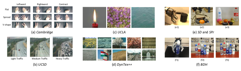
Figure 3: Samples of the benchmark datasets. (a) Cambridge: the image sequences are performed by $3$ primitive hand shapes with $3$ primitive motions; (b) UCSD: representative examples of the three classes; (c) UCLA: candle, flower and Sea; (d) DynTex++: flowers, sea, naked trees, foliage, escalator, calm water, flags, grass, traffic, and fountains; (e) SD and SPr: (e1) the 3-finger Schunk Dextrous hand, (e2) the 2-finger Schunk Parallel hand, (e3) objects in SD and SPr including rubber ball, balsam bottle, rubber duck, empty bottle, full bottle, bad orange, rresh orange, joggling ball, tape, and wood block; (f) BDH: (f1) the BH8-280 Hand, (f2) bottles without water, (f3) bottles with water.

9.1 Benchmark Datasets

We consider two types of benchmark datasets, namely vision datasets and tactile datasets in our experiments. The specification of each dataset is provided in Table 3.

Vision datasets

As for the vision tests, we make use of four widely used datasets, namely, Cambridge, UCSD, UCLA, and DynTex++ (see Fig. 3 for examples).

Cambridge. The Cambridge hand gesture dataset Kim and Cipolla (2009) consists of $900$ images sequences of $9$ gesture classes generated by $3$ primitive hand shapes and $3$ primitive motions. Each class contains $100$ image sequences performed by $2$ subjects, with $10$ arbitrary camera motions and under $5$ illumination conditions. Sample images are demonstrated in Fig. 3 (a). Similar to Harandi and Salzmann (2015), we resize all images to $20\times 20$, and use the first $80$ images of each class for testing while the remaining images are used for training purposes.

UCSD. The experiment of scene analysis is performed using the UCSD traffic dataset Chan and Vasconcelos (2005) (see Fig. 3 (b) for sample images). UCSD dataset consists of 254 video sequences of highway traffic with a variety of traffic patterns in various weather conditions. Each video is recorded with a resolution of $320\times 240$ pixels for a duration between $42$ and $52$ frames. We use the cropped version of the dataset where each video is cropped and resized to $48\times 48$. The dataset is labeled into three classes with respect to the severity of traffic congestion in each video. The total number of sequences with heavy, medium and light traffic is 44, 45 and 165, respectively. We use the four splits suggested in Chan and Vasconcelos (2005) in our tests.

UCLA. The UCLA dataset Saisan et al. (2001) contains 50 categories of dynamic textures (see Fig. 3 (c) for sample images). Each category consists of 4 gray-scale videos captured from different viewpoints. Each video has 75 frames and cropped to $48\times 48$ by keeping the associated motion. Four random splits of the dataset, as provided in Saisan et al. (2001) are used in our experiments.

DynTex++. Dynamic textures are video sequences of complex scenes that exhibit certain stationary properties in the time domain, such as water on the surface of a lake, a flag fluttering in the wind, swarms of birds, humans in crowds, etc. The constant change poses a challenge for applying traditional vision algorithms to these videos. The dataset DynTex++ Ghanem and Ahuja (2010) (see Fig. 3 (d) for sample images) is a variant of the original DynTex Péteri et al. dataset. It contains $3600$ videos of $36$ classes ($100$ videos of size $50\times 50\times 50$ per class). In this paper, we apply the same test protocol as Ghanem and Ahuja (2010), namely, half of the videos are applied as the training set and the other half as the testing set over 10 trials. We utilize the histogram of LBP from Three Orthogonal Planes (LBP-TOP) Zhao and Pietikainen (2007) as the input feature by splitting each video into sub-videos of length $8$, with a 6-frame overlap.

Tactile datasets

Recognizing objects that a robot grasps via the tactile series is an active research area in robotics Madry et al. (2014). The tactile series obtained from the force sensors can be used to determine properties of an object (e.g., shape or softness). In our experiments, the recognition tasks are evaluated on three datasets: namely SD Yang et al. (2015), SPr Madry et al. (2014) and BDH Madry et al. (2014). The SD dataset contains $100$ tactile series of $10$ household objects grasped by a 3-finger Schunk Dextrous (SD) hand. The SPr dataset composed of $97$ sequences with the same object classes as SD, but is captured with a 2-finger Schunk Parallel (SPr) hand (see Fig. 3 (e) for sample images). BDH consists of $100$ tactile sequences generated by controlling the BH8-280 Hand to grasp $5$ different bottles with water or without water (see Fig. 3 (f) for sample images). The task is to predict whether the bottle is empty or is filled with water. All datasets are split randomly into the training and testing sets with a ratio of $9:1$ over $10$ trials Madry et al. (2014); Yang et al. (2015).

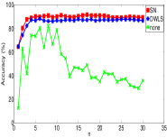
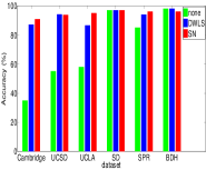
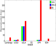
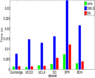
Figure 4: Comparisons between stable and non-stable LDSs. The left panel shows the average classification accuracies for non-stable LDSs (denoted by none) and stabilized LDSs by SN and DWLS methods on the Cambridge dataset. The horizontal axis represents the state dimensionality $n$ here. The second panel from left shows the average classification accuracies for the Cambridge, UCSD, UCLA, SD, SPR, and BDH datasets with $n=20$. The third and fourth diagrams show the average reconstruction errors and average learning times for the studied datasets. The parameter $a$ in SN is set to $4$ for the UCSD, UCLA, SD, SPR and BDH datasets and $2.5$ for the Cambridge dataset.

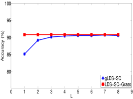
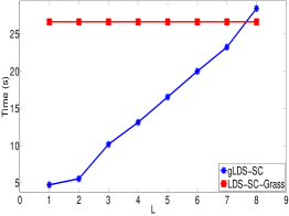
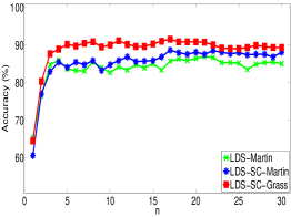
Figure 5: Performance of the proposed sparse coding methods on Cambridge. (a) The classification accuracies of LDS-SC-Grass and gLDS-SC versus observability order $L$ (here, $n=20$). (b) Training time of LDS-SC-Grass and gLDS-SC versus the observability order $L$. (c) Performances of LDS-Martin, LDS-SC-Martin and LDS-SC-Grass versus state dimensionality $n$.

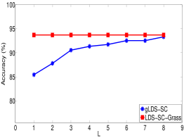
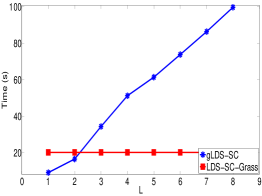
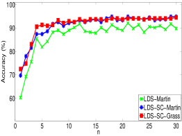
Figure 6: Performance of the proposed sparse coding methods on UCSD. (a) The classification accuracies of LDS-SC-Grass and gLDS-SC versus observability order $L$ (here, $n=20$). (b) Training time of LDS-SC-Grass and gLDS-SC versus the observability order $L$. (c) Performances of LDS-Martin, LDS-SC-Martin and LDS-SC-Grass versus state dimensionality $n$.

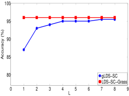
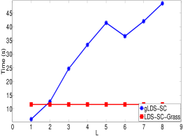
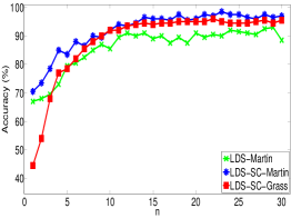
Figure 7: Performance of the proposed sparse coding methods on the UCLA dataset. (a) The classification accuracies of LDS-SC-Grass and gLDS-SC versus observability order $L$ (here, $n=20$). (b) Training time of LDS-SC-Grass and gLDS-SC versus the observability order $L$. (c) Performances of LDS-Martin, LDS-SC-Martin and LDS-SC-Grass versus state dimensionality $n$.

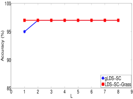
Figure 8: Performance of the proposed sparse coding methods on SD. (a) The classification accuracies of LDS-SC-Grass and gLDS-SC versus observability order $L$ (here, $n=20$). (b) Training time of LDS-SC-Grass and gLDS-SC versus the observability order $L$. (c) Performances of LDS-Martin, LDS-SC-Martin and LDS-SC-Grass versus state dimensionality $n$.

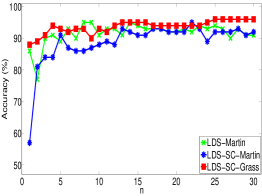
Figure 9: Performance of the proposed sparse coding methods on SPR. (a) The classification accuracies of LDS-SC-Grass and gLDS-SC versus observability order $L$ (here, $n=20$). (b) Training time of LDS-SC-Grass and gLDS-SC versus the observability order $L$. (c) Performances of LDS-Martin, LDS-SC-Martin and LDS-SC-Grass versus state dimensionality $n$.

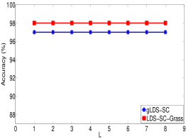
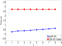
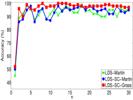
Figure 10: Performance of the proposed sparse coding methods on BDH. (a) The classification accuracies of LDS-SC-Grass and gLDS-SC versus observability order $L$ (here, $n=20$). (b) Training time of LDS-SC-Grass and gLDS-SC versus the observability order $L$. (c) Performances of LDS-Martin, LDS-SC-Martin and LDS-SC-Grass versus state dimensionality $n$.

Table 4: Averaged classification accuracies of the proposed sparse coding methods compared with the state-of-the-arts.

Datasets	References	LDS-SVM	LDS-Martin	Proposed models
				Our best	LDS-SC-Martin	LDS-SC-Grass
Cambridge	90.71 ; 83.12	86.5	86.9	91.7	88.6	91.7
UCSD	94.53 ; 87.84	94.5	92.1	94.9	94.9	94.5 9
UCLA	96.03 ; 97.55	95.0	93.0	98.5	98.5	96.0
SD	976 ; 927	98	95	98	97	98
SPR	916 ; 897	94	95	96	95	96
BDH	816 ; 878	80	98	100	98	100

• KSLCC: Harandi and Salzmann (2015).

• SSSC: Mahmood et al. (2014).

• KL-SVM: Chan and Vasconcelos (2005).

• CS-LDS: Sankaranarayanan et al. (2013).

• KDT-SVM: Chan and Vasconcelos (2007).

• ST-HMP: Madry et al. (2014).

• DTW: Drimus et al. (2014).

• JKSC: Yang et al. (2015).

• The result of LDS-SC-Grass on UCSD is better than our earlier work Huang et al. (2016b), as here we employe the SN stabilization before coding while in Huang et al. (2016b) we simply stabilize $A$ by dividing it with a scale factor.

9.2 Sparse coding

In this part, we assess the performance of the proposed sparse coding techniques by constructing the LDS dictionary directly from the training data, meaning each atom in the dictionary is one sample from the training set. Classification is done using the approach presented in § 5.3. The experiments are carried out on Cambridge, UCSD, UCLA, SD, SPR, and BDH.

Non-stable vs. Stable. We start by studying the stability procedure proposed in § 4.2 for classification purposes. Thus, we extract dynamical features in two different ways: one with and one without SN. Though our SN method avoids any optimization procedure, it is interesting to compare it against optimization-based methods to show its full potential. Among LDS stabilization methods that benefit from optimization techniques, WLS shows to be fast while achieving small reconstruction errors Huang et al. (2016a). Here, we only consider the diagonal form of WLS, i.e., DWLS. The stable bound in DWLS is set to 0.99 to make the computation of the Lyapunov equation possible. The exacted features are fed to LDS-SC-Grass for classification. As shown in Fig. 4, stabilization can promote the classification accuracies on Cambridge, UCSD, UCLA, SPR datasets while not helping on SD and BDH datasets. In terms of the state reconstruction errors (see Huang et al. (2016a) for details), SN underperforms in comparison to DWLS. However, when classification accuracy is considered, SN generally yields better results while being remarkably faster. We conjecture that SN can preserve the discriminative information contained in the data sequences. Based to the results here, we will only perform SN on Cambridge, UCSD, UCLA, SPR datasets in the following experiments.

Infinite vs. Finite.
As discussed in § 5, LDS-SC-Grass can be understood as a generalization of gLDS-SC from finite-dimensional Grassmannian to infinite Grassmannian. Here, we are interested in the asymptotic behavior of gLDS-SC when the observability order $L$ increases. For this purpose, we report the results in Figures 5-10. As expected, the classification accuracy of gLDS-SC converges to that of LDS-SC when $L$ increases. In § 8, we have shown that the computational complexity of gLDS-SC ($O(L(NJ+J^{2})mn^{2})$) is $L$ times more than that of LDS-SC ($O((NJ+J^{2})mn^{2})$). Larger $L$ demands for more computational resources in gLDS-SC. As shown in Fig. 7 (b), gLDS-SC takes more coding time than LDS-SC when $L>2$. On tactile datasets, LDS-SC-Grass performs much slower than gLDS-SC when $L<8$. This is because LDS-SC-Grass additionally requires SVD decomposition and solving the Lyapunov equation, both are $O(n^{3})$ computation-wise. When the dimensions of the data $m$ is large (e.g., UCSD and UCLA datasets), additional computations have a small impact in the coding time.

Varying $n$.
To evaluate the sensitivity of the coding algorithms with respect to the hidden dimensionality (i.e., $n$), we performed an experiment using LDS-Martin, LDS-SC-Martin and LDS-SC-Grass methods. From Fig. 7 (c), we can see that the proposed methods, i.e., LDS-SC-Martin and LDS-SC-Grass, perform consistently when $n$ is greater than a certain value. Also both proposed methods outperform the LDS-Martin when $n$ is sufficiently large. LDS-SC-Martin performs better than LDS-SC-Grass on UCLA and UCSD, indicating that applying a Gaussian kernel plus Martin distance on these two datasets is beneficial. However, on other datasets (including all the tactile datasets), LDS-SC-Grass is better than LDS-SC-Martin. The take-home message here is that, while employing different kernel functions can lead to slight improvements, sparse coding is a robust and powerful method for analyzing LDSs.

Comparison with the state-of-the-art.
We compare the proposed sparse coding methods, i.e., LDS-SC-Martin and LDS-SC-Martin, against the state-of-the-art in this part. Beside the dataset-dependent state-of-the-arts, we use two baselines, namely LDS-Martin and LDS-SVM. For the proposed methods and also LDS-Martin and LDS-SVM, we vary the parameter $n$ and report the best results in Table 4. We first note that the best results of our proposed algorithms outperform all other baselines and state-of-the-arts on all datasets. On the UCSD dataset, the method proposed in Chan and Vasconcelos (2005) achieves a similar performance to that of LDS-SC-Martin. As discussed in our preliminary study Huang et al. (2016b), one can combine the state covariance term into the sparse coding formulation (see Eq. (25)) to boost the accuries more. With such combination, the accuracy of LDS-SC-Grass increases from 98% and 96% to 100% and 97% on the SD and SPR datasets, respectively.

9.3 Dictionary learning

In this part, we analyze the effectiveness of the proposed dictionary learning algorithms. Experiments are carried out on the Cambridge and DynTex++ datasets. For the Cambridge dataset, we considered a different testing protocol compared to that of the sparse coding. In particular, we split the videos of each class into two non-overlapping and equal-sized sets and used the first half for learning the dictionary. The random splitting is repeated $10$ times and the average accuracies over $10$ trials are reported here. The sparse codes for training and test data with respect to a learned dictionary are fed to a linear SVM Fan et al. (2008) for classification. The parameter $n$ is fixed to $10$ in all the experiments.

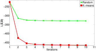
Figure 11: The cost of LDS-DL with Algorithm 1 on Cambridge. The vertical axis represents the cost (Eq. (20)) and the horizontal axis denotes the iteration number where each iteration refers to a complete update of all dictionary atoms. $J=8$.

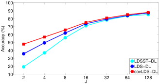
Figure 12: Comparison between LDSST-DL, LDS-DL and covLDS-DL with varying values of $J$ on Cambridge. For covLDS-DL, $\beta=0.2$.

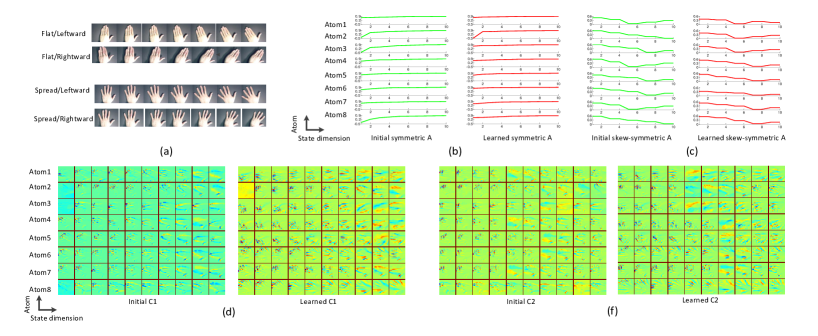
Figure 13: Visualization of the initial and the learned dictionaries on Cambridge. $J=8$. (a) Samples of the $4$ sub-categories in Cambridge. (b-c) Plots of ${\boldsymbol{A}}$: different plots display the values of the transition eigenvalues of different atoms; (d-f) Visualization of A: rows corresponds to atoms and columns to the state dimensions.

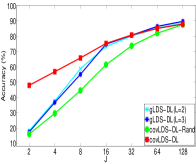
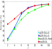
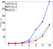
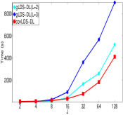
Figure 14: Comparisons between covLDST-DLs and gLDS-DLs for various dictionary size $J$ on the Cambridge and DynTex++ (the $9$-classes subset) datasets. The first two panels show the average classification accuracies, while the right two ones display the training time for a one update of all atoms.

Convergence analysis.
At each step of our dictionary learning algorithm (Algorithm 1), the updated columns of the measurement matrices are optimal according to Theorems 5 and 6. Each diagonal element of the transition matrices is updated in the opposite direction of the gradient, thus reducing the cost function. To further show this, we randomly initialize the dictionary atoms with the training data and plot the convergence behavior of LDS-DL in Fig. 11. This plot suggests that the algorithm convergences in a few iterations.

In addition to random initialization, we are also interested in developing a K-means-like approach to cluster data sequences prior to dictionary learning. Once such mechanism is at our disposal, we can make use of the clustering centers to initialize the dictionary. Recalling that the traditional K-means paradigm consists of two alternative phases: first assigning the data to the closest centers under the given distance metric and then updating the centers with the new assigned data Bishop et al. (2006). Extending the first step is straightforward for LDS clustering; the second one entails a delicate method for computing the clustering centers. Suppose the extended observability subspaces in a cluster are $\{{\boldsymbol{V}}_{i}\}_{i=1}^{q}$. We define the center of this set as ${\boldsymbol{V}}_{c}=\arg\min_{{\boldsymbol{V}}_{c}}\parallel{\boldsymbol{V}}_{c}{\boldsymbol{V}}_{c}^{\mathrm{T}}-\frac{1}{q}\sum_{i=1}^{q}{\boldsymbol{V}}_{i}{\boldsymbol{V}}_{i}^{\mathrm{T}}\parallel_{F}^{2}$. Unfolding this equation actually leads to a special case of Eq. (15) by setting the number of the dictionary atoms $J$ to be 1 and the values of the codes ${\boldsymbol{Z}}_{i,r}$ to $1/q$. This means that we can calculate the system tuples of the centers with Algorithm 1. The convergence curve of LDS-DL with the K-means initialization is shown in Fig. 11. We find that the objective decreases significantly after the K-means initialization, leading to superior performances compared to random initialization. Thus, in the following experiments, we employ K-means to initialize the dictionary unless mentioned otherwise.

To learn an LDS dictionary, our preliminary study Huang et al. (2016b) opts for symmetric LDSs to model data. In this study, we introduce the notion of a two-fold LDS, decomposing an LDS into symmetric and screw-symmetric parts. In Fig. 12, we compare the two methods, namely LDSST-DL and LDS-ST, on the Cambridge dataset for various size of dictionary. This experiment shows the superiority of LDS-DL over LDSST-DL. In § 7, we show how to consider the state covariances for learning a more discriminative dictionary. As shown in Fig. 12, equipping LDS-DL with state covariances, i.e., covLDS-DL, can further boost the performances.

Visualizing the Dictionary.
The LDS-DL algorithm learns the measurement (i.e., ${\boldsymbol{C}}$) and the transition (i.e., ${\boldsymbol{A}}$) matrices explicitly and separately. Thus, we can visualize the learned system tuples $({\boldsymbol{A}},{\boldsymbol{C}})$ to demonstrate what patterns have been captured. For simplicity, we perform LDS-DL on the $4$-class subset of Cambridge, namely, Flat-Leftward, Flat-Rightward, Spread-Leftward, and Spread-Rightward. Dictionary atoms are initialized randomly by choosing $8$ videos from the class Flat-Leftward.

Fig. 13 (a) visualizes both the initial and the learned pairs. As the system tuples of the skew-symmetric dictionary are complex, we visualize the corresponded real pairs, i.e., $({\boldsymbol{\Theta}},{\boldsymbol{Q}})$. Clearly, more spatial patterns such as the spread-hand shape and the hand-rightward state, have been captured by the learned measurement matrices. There are also slight changes in transition matrices after training. The transition matrices of different atoms have a small difference, indicating that there is not much dynamic, presumably because the speed of hand and the sampling frequency of the camera are consistent.

Is training useful?
To verify whether learning a dictionary is helpful towards classification purposes or not, we compare covLDS-DL against a baseline, namely covLDS-Rand, in which the dictionary atoms are chosen from the training set randomly (no training is involved). In addition to covLDS-Rand, we use gLDS-DL with $L=2,3$ as another baseline. For fair comparisons, we use a linear SVM and set $n=10$ for covLDS-DL, covLDS-Rand and gLDS-DL.

To compare covLDS-DL with covLDS-Rand and gLDS-DL, we use the Cambridge and a smaller subset of DynTex++ dataset (only the videos from the first $9$ classes). By cross-validation, $\beta$ is 0.2 in the Cambridge and 0.8 in the DynTex++ dataset in covLDS-DL. Fig. 14 shows that covLDS-DL consistently outperforms covLDS-Rand for various number of the dictionary atoms. Compared to gLDS-DLs, covLDS-DL achieves higher accuracies when the dictionary size $J$ is small (e.g., $J<16$), and obtains on par performances when $J$ is large. As discussed in § 7, the computational complexity of gLDS-DL is higher than covLDS-DL. We also plot the training time of gLDS-DLs and covLDS-DL in Fig. 14, showing that gLDS-DL is more computationally exhaustive as $L$ increases.

In addition to the $9$-classes subset, we also evaluate LDS-DL on the whole DynTex++ dataset. To speed up the convergence rate, we learn the dictionary in a hierarchical manner, i.e., separately learning $J_{c}$ dictionary atoms for each class. Fig. 15 shows the performance of the hierarchical dictionary for various values of $J_{c}$. LDS-DL achieves the accuracy of $91.7\%$ when $J_{c}=32$, which is better than that of the Grassmaniann-based method (i.e., $90.3\%$) Harandi et al. (2013) and comparable to Grassmannian-kernel-based method (i.e., $92.8\%$) Harandi et al. (2013). By choosing $J_{c}=50$ the classification accuracy increases to $93.06\%$ (see Fig. 15).

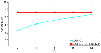
Figure 15: Classification performance on the DynTex++ dataset.

10 Conclusion

In this paper, we address several shortcomings in modeling Linear Dynamical Systems (LDS). In particular, we formulate the extended observability subspace of an LDS explicitly and devise an efficient method called SN to stabilize LDSs. We then tackle two challenging problems, namely LDS coding and learning an LDS dictionary. In the former, the goal is to describe an LDS with a sparse combination of a set of LDSs, known as a dictionary. In the latter, we show how an LDS dictionary can be obtained from a set of LDSs. Towards solving the aforementioned problems, we introduce the novel concept of two-fold LDSs and make use of it to obtain closed-form updates for learning an LDS dictionary. Our extensive set of experiments shows the superiority of the proposed techniques compared to various state-of-the-art methods on different tasks including hand gesture recognition, dynamical scene classification, dynamic texture categorization and tactile recognition.

A Proofs

We present the proofs of Theorems 1-6. For better readability, we repeat the theorems before the proofs.

Theorem 1

Suppose ${\boldsymbol{V}}_{1},{\boldsymbol{V}}_{2},\cdots,{\boldsymbol{V}}_{M}\in\mathcal{S}(n,\infty)$, and $y_{1},y_{2},\cdots,y_{M}\in\mathbb{R}$, we have

$$\parallel\sum_{i=1}^{M}y_{i}\Pi({\boldsymbol{V}}_{i})\parallel_{F}^{2} = \sum_{i,j=1}^{M}y_{i}y_{j}\parallel{\boldsymbol{V}}_{i}^{\mathrm{T}}{\boldsymbol{V}}_{j}\parallel_{F}^{2},$$

Proof  We denote the $t$-order sub-matrix of the extended observability matrix ${\boldsymbol{O}}_{i}$ as ${\boldsymbol{O}}_{i}(t)=[{\boldsymbol{C}}_{i}^{\mathrm{T}},({\boldsymbol{C}}_{i}{\boldsymbol{A}}_{i})^{\mathrm{T}},\cdots,({\boldsymbol{C}}_{i}{\boldsymbol{A}}_{i}^{t})]^{\mathrm{T}}$. Suppose the factored matrix for orthogonalizing ${\boldsymbol{O}}_{i}$ is ${\boldsymbol{L}}_{i}$ (see §4.3 in the paper) and denote that ${\boldsymbol{V}}_{i}(t)={\boldsymbol{O}}_{i}(t){\boldsymbol{L}}_{i}^{\mathrm{-T}}$. Then, we derive

$$\parallel\sum_{i=1}^{M}y_{i}\Pi({\boldsymbol{V}}_{i})\parallel_{F}^{2}$$

$$=\lim_{t\rightarrow\infty}\parallel\sum_{i=1}^{M}y_{i}{\boldsymbol{V}}_{i}(t){\boldsymbol{V}}_{i}(t)^{\mathrm{T}}\parallel_{F}^{2}$$

$$=\lim_{t\rightarrow\infty}\mathrm{Tr}\left(\sum_{i=1}^{M}y_{i}{\boldsymbol{V}}_{i}(t){\boldsymbol{V}}_{i}(t)^{\mathrm{T}}\sum_{j=1}^{J}y_{j}{\boldsymbol{V}}_{j}(t){\boldsymbol{V}}_{j}(t)^{\mathrm{T}}\right)$$

$$=\lim_{t\rightarrow\infty}\sum_{i,j=1}^{M}y_{i}y_{j}\mathrm{Tr}\left({\boldsymbol{V}}_{i}(t)^{\mathrm{T}}{\boldsymbol{V}}_{j}(t){\boldsymbol{V}}_{j}(t)^{\mathrm{T}}{\boldsymbol{V}}_{i}(t)\right)$$

$$=\sum_{i,j=1}^{M}y_{i}y_{j}\lim_{t\rightarrow\infty}\parallel{\boldsymbol{V}}_{i}(t)^{\mathrm{T}}{\boldsymbol{V}}_{j}(t)\parallel_{F}^{2}$$

$$=\sum_{i,j=1}^{M}y_{i}y_{j}\lim_{t\rightarrow\infty}\parallel{\boldsymbol{L}}_{i}^{-1}({\boldsymbol{O}}_{i}(t)^{\mathrm{T}}{\boldsymbol{O}}_{j}(t)){\boldsymbol{L}}_{j}^{\mathrm{-T}}\parallel_{F}^{2}$$

$$=\sum_{i,j=1}^{M}y_{i}y_{j}\parallel{\boldsymbol{L}}_{i}^{-1}{\boldsymbol{O}}_{ij}{\boldsymbol{L}}_{j}^{\mathrm{-T}}\parallel_{F}^{2},$$ (25)

where the limitation value ${\boldsymbol{O}}_{ij}=\lim_{t\rightarrow\infty}{\boldsymbol{O}}_{i}(t)^{\mathrm{T}}{\boldsymbol{O}}_{j}(t)={\boldsymbol{O}}_{i}^{\mathrm{T}}{\boldsymbol{O}}_{j}$ exists and is computed by solving the Lyapunov equation similar to Eq. (4).  

Corollary 2

For any ${\boldsymbol{V}}_{1},{\boldsymbol{V}}_{2}\in\mathcal{S}(n,\infty)$, we have

$$\|\Pi({\boldsymbol{V}}_{1})-\Pi({\boldsymbol{V}}_{2})\|_{F}^{2} = 2\left(n-\|{\boldsymbol{V}}_{1}^{\mathrm{T}}{\boldsymbol{V}}_{2}\|_{F}^{2}\right).$$

Furthermore, $\|\Pi({\boldsymbol{V}}_{1})-\Pi({\boldsymbol{V}}_{2})\|_{F}^{2}=2\sum_{k=1}^{n}\sin^{2}\alpha_{k}$, where $\{\alpha_{k}\}_{k=1}^{n}$ are subspace angles between ${\boldsymbol{V}}_{1}$ and ${\boldsymbol{V}}_{2}$. This also indicates that $0\leq\|\Pi({\boldsymbol{V}}_{1})-\Pi({\boldsymbol{V}}_{2})\|_{F}^{2}\leq 2n$.

The Frobenius distance $\parallel\Pi({\boldsymbol{V}}_{1})-\Pi({\boldsymbol{V}}_{2})\parallel_{F}^{2}$ is devised by setting $y_{1}=1$ and $y_{2}=-1$ in Eq. (A). As demonstrated in Harandi et al. (2013), the embedding $\Pi({\boldsymbol{V}})$ from the finite Grassmannian $\mathcal{G}(n,d)$ to the space of the symmetric matrices is proven to be diffeomorphism (a one-to-one, continuous, and differentiable mapping with a continuous and differentiable inverse); The Frobenius distance between the two points ${\boldsymbol{V}}_{1}$ and ${\boldsymbol{V}}_{2}$ in the embedding space can be rewritten as

$$\parallel{\boldsymbol{V}}_{1}{\boldsymbol{V}}_{1}^{\mathrm{T}}-{\boldsymbol{V}}_{2}{\boldsymbol{V}}_{2}^{\mathrm{T}}\parallel_{F}^{2}=2\sum_{k=1}^{n}\sin^{2}\alpha_{k},$$ (26)

where $\alpha_{k}$ is the $k$-th principal angle of the subspaces between ${\boldsymbol{V}}_{1}$ and ${\boldsymbol{V}}_{2}$.

We denote the space of the finite observability subspaces as $\mathcal{S}(n,L)$ by taking the first $L$ rows from the extended observability matrix. Clearly, $\mathcal{S}(n,L)$ is a compact subset of $\mathcal{G}(n,L)$. Hence $\mathcal{S}(n,L)$ maintains the relation in Eq. (26); and the embedding $\Pi({\boldsymbol{V}})$ from $\mathcal{S}(n,L)$ to the space of the symmetric matrices is diffeomorphism. For our case, $\mathcal{S}(n,\infty)=\lim_{L\rightarrow\infty}\mathcal{S}(n,L)$. Theorem (1) proves the Frobenius distance defined in the embedding $\Pi(\mathcal{S}(n,\infty))$ to be convergent. Thus, we can obtain the relation between the Frobenius distance and the subspace angles in Corollary 2, and prove that the embedding $\Pi(\mathcal{S}(n,\infty))$ is diffeomorphism, by extending the conclusions of $\mathcal{S}(n,L)$ with $L$ approaching to the infinity.

Lemma 3

For a symmetric or skew-symmetric transition matrix ${\boldsymbol{A}}$, the system tuple $({\boldsymbol{A}},{\boldsymbol{C}})\in\mathbb{R}^{n\times n}\times\mathbb{R}^{m\times n}$ has the canonical form $({\boldsymbol{\Lambda}},{\boldsymbol{U}})\in\mathbb{R}^{n}\times\mathbb{R}^{m\times n}$, where ${\boldsymbol{\Lambda}}$ is diagonal and ${\boldsymbol{U}}$ is unitary, i.e. ${\boldsymbol{U}}^{\ast}{\boldsymbol{U}}={\boldsymbol{I}}$. Moreover, both ${\boldsymbol{\Lambda}}$ and ${\boldsymbol{U}}$ are real if ${\boldsymbol{A}}$ is symmetric and complex if ${\boldsymbol{A}}$ is skew-symmetric; for the skew-symmetric ${\boldsymbol{A}}$, $({\boldsymbol{\Lambda}},{\boldsymbol{U}})$ is parameterized by a real matrix-pair $({\boldsymbol{\Theta}},{\boldsymbol{Q}})\in\mathbb{R}^{n}\times\mathbb{R}^{m\times n}$ where ${\boldsymbol{\Theta}}$ is diagonal and ${\boldsymbol{Q}}$ is orthogonal, and $n$ is even.

Proof  A symmetric or skew-symmetric matrix ${\boldsymbol{A}}$ can be decomposed as ${\boldsymbol{A}}={\boldsymbol{U}}{\boldsymbol{\Lambda}}{\boldsymbol{U}}^{\ast}$ Nor ; Ske . Here ${\boldsymbol{U}}$ is a unitary matrix and ${\boldsymbol{\Lambda}}$ is a diagonal matrix storing the eigenvalues of ${\boldsymbol{A}}$. Due to the invariance property of the system tuple, we attain that

$$({\boldsymbol{A}},{\boldsymbol{C}}) = ({\boldsymbol{U}}{\boldsymbol{\Lambda}}{\boldsymbol{U}}^{\ast},{\boldsymbol{C}}),$$

$$\sim ({\boldsymbol{\Lambda}},{\boldsymbol{C}}{\boldsymbol{U}}),$$

$$= ({\boldsymbol{\Lambda}},{\boldsymbol{U^{\prime}}}),$$ (28)

with “$\sim$” denoting the equivalence relation. Clearly, ${\boldsymbol{U^{\prime}}}$ is also unitary. Thus, we ignore the difference between ${\boldsymbol{U^{\prime}}}$ and ${\boldsymbol{U}}$ for consistency, and denote ${\boldsymbol{U^{\prime}}}$ as ${\boldsymbol{U}}$ in the following context.

In particular, for a symmetric matrix, both ${\boldsymbol{U}}$ and ${\boldsymbol{\Lambda}}$ are real; for an skew-symmetric matrix, the diagonal elements of ${\boldsymbol{\Lambda}}$ and the columns of ${\boldsymbol{U}}$ are

$$[{\boldsymbol{\Lambda}}]_{2k-1}=[{\boldsymbol{\Theta}}]_{k}\cdot 1i;~{}~{}~{}[{\boldsymbol{\Lambda}}]_{2k}=-[{\boldsymbol{\Theta}}]_{k}\cdot 1i,$$ (29)

and

$$\left\{\begin{array}[]{lll}&\left[{\boldsymbol{U}}\right]_{2k-1}&=\frac{1}{\sqrt{2}}[{\boldsymbol{Q}}]_{2k-1}+\frac{1i}{\sqrt{2}}[{\boldsymbol{Q}}]_{2k},\\ &\left[{\boldsymbol{U}}\right]_{2k}&=\frac{1}{\sqrt{2}}[{\boldsymbol{Q}}]_{2k-1}-\frac{1i}{\sqrt{2}}[{\boldsymbol{Q}}]_{2k},\end{array}\right.$$ (32)

for $k=1,2,\cdots,\frac{n}{2}$ if $n$ is even, where ${\boldsymbol{\Theta}}\in\mathbb{R}^{\frac{n}{2}\times\frac{n}{2}}$ is a real diagonal matrix and ${\boldsymbol{Q}}\in\mathbb{R}^{m\times n}$ is a real orthogonal matrix. Thus $({\boldsymbol{\Lambda}},{\boldsymbol{U}})$ can be parameterized by $({\boldsymbol{\Theta}},{\boldsymbol{Q}})$ which is of real value.  

Theorem 4

For the two-fold LDS modeling defined in Eq. (17), the sup-problem in Eq. (16) is equivalent to

$$\begin{aligned} &\min_{{\boldsymbol{U}}_{r}^{(d)},{\boldsymbol{\Lambda}}_{r}^{(d)}}&&\sum_{k=1}^{n}[{\boldsymbol{U}}_{r}^{(d)}]_{k}^{*}{\boldsymbol{S}}_{r,k}[{\boldsymbol{U}}_{r}^{(d)}]_{k}\\ &~{}~{}~{}\mathrm{s.t.}&&({\boldsymbol{U}}_{r}^{(d)})^{*}{\boldsymbol{U}}_{r}^{(d)}=\mathbf{I}_{n};\\ &&&-1<[{\boldsymbol{\Lambda}}_{r}^{(d)}]_{k}<1,~{}1\leq k\leq n.\end{aligned}$$ (33)

Here, the matrix ${\boldsymbol{S}}_{r,k}$ (see Table 2) is not dependent on the measurement matrix ${\boldsymbol{U}}_{r}^{(d)}$.

Proof  We first derive several preliminary results prior to the proof of this theorem.

In the conventional LDS modeling, the exact form of the self-inner-product on extended observability matrices cannot be obtained due to the implicit calculation of the Lyapunov equation (Eq. (4)). Thanks to Lemma 3, the system tuple with symmetric or skew-symmetric transition matrix has the canonical representation $({\boldsymbol{\Lambda}},{\boldsymbol{U}})$ where ${\boldsymbol{\Lambda}}$ is diagonal and ${\boldsymbol{U}}$ is unitary. Then, the self-inner-product of the corresponding extended observability matrix is computed as

$${\boldsymbol{O}}^{\mathrm{T}}{\boldsymbol{O}} = \sum_{t=0}^{\infty}({\boldsymbol{\Lambda}}^{*})^{t}{\boldsymbol{\Lambda}}^{t},$$ (34)

$$= \mathrm{diag}([\frac{1}{1-|\lambda_{1}|^{2}},\frac{1}{1-|\lambda_{2}|^{2}},\cdots,\frac{1}{1-|\lambda_{n}|^{2}}]),$$

where $\lambda_{k}=[{\boldsymbol{\Lambda}}]_{k}$.

Further considering the SVD factorization ${\boldsymbol{O}}^{\mathrm{T}}{\boldsymbol{O}}={\boldsymbol{U}}_{o}{\boldsymbol{S}}_{o}{\boldsymbol{U}}_{o}^{\mathrm{T}}$, the factor matrix is obtained as ${\boldsymbol{L}}={\boldsymbol{U}}_{o}{\boldsymbol{S}}_{o}^{1/2}=\mathrm{diag}([\frac{1}{(1-|\lambda_{1}|^{2})^{1/2}},\frac{1}{(1-|\lambda_{2}|^{2})^{1/2}},\cdots,\frac{1}{(1-|\lambda_{n}|^{2})^{1/2}}])$. The orthogonal extended observability matrix is given by ${\boldsymbol{V}}={\boldsymbol{O}}{\boldsymbol{L}}^{-\mathrm{T}}$.

For simplicity, we here denote the canonical representation, the factor matrix and the extended observability subspace for dictionary atom ${\boldsymbol{D}}_{j}$ as $({\boldsymbol{\Lambda}}_{j},{\boldsymbol{U}}_{j})$, ${\boldsymbol{L}}_{j}$ and ${\boldsymbol{V}}_{j}$, respectively, by omitting the superscript ^(d). The kernel between dictionary atoms in Eq. (15) is devised as

$$K({\boldsymbol{D}}_{r},{\boldsymbol{D}}_{j})$$ (35)

$$= \parallel{\boldsymbol{V}}_{r}^{\mathrm{T}}{\boldsymbol{V}}_{j}\parallel_{F}^{2}$$

$$= \parallel{\boldsymbol{L}}_{r}^{-1}\sum_{t=0}^{\infty}({\boldsymbol{\Lambda}}_{r}^{*})^{t}{\boldsymbol{U}}_{r}^{*}{\boldsymbol{U}}_{j}{\boldsymbol{\Lambda}}_{j}^{t}{\boldsymbol{L}}_{j}^{-\mathrm{T}}\parallel_{F}^{2}$$

$$= \mathrm{Tr}\left({\boldsymbol{L}}_{r}^{-1}\left(\sum_{t_{1}=0}^{\infty}({\boldsymbol{\Lambda}}_{r}^{*})^{t_{1}}{\boldsymbol{U}}_{r}^{*}{\boldsymbol{U}}_{j}{\boldsymbol{\Lambda}}_{j}^{t_{1}}\right){\boldsymbol{L}}_{j}^{-\mathrm{T}}{\boldsymbol{L}}_{j}^{-1}\left(\sum_{t_{2}=0}^{\infty}({\boldsymbol{\Lambda}}_{j}^{*})^{t_{2}}{\boldsymbol{U}}_{j}^{*}{\boldsymbol{U}}_{r}{\boldsymbol{\Lambda}}_{r}^{t_{2}}\right){\boldsymbol{L}}_{r}^{-\mathrm{T}}\right)$$

$$= \sum_{t_{1}=0}^{\infty}\sum_{t_{2}=0}^{\infty}\mathrm{Tr}\left({\boldsymbol{L}}_{r}^{-1}({\boldsymbol{\Lambda}}_{r}^{*})^{t_{1}}){\boldsymbol{U}}_{r}^{*}{\boldsymbol{U}}_{j}{\boldsymbol{\Lambda}}_{j}^{t_{1}}({\boldsymbol{L}}_{j}^{-\mathrm{T}}{\boldsymbol{L}}_{j}^{-1})({\boldsymbol{\Lambda}}_{j}^{*})^{t_{2}}{\boldsymbol{U}}_{j}^{*}{\boldsymbol{U}}_{r}(({\boldsymbol{\Lambda}}_{r})^{t_{2}}{\boldsymbol{L}}_{r}^{-\mathrm{T}})\right)$$

$$= \sum_{t_{1}=0}^{\infty}\sum_{t_{2}=0}^{\infty}\sum_{k=1}^{n}(1-|\lambda_{r,k}|^{2})^{\frac{1}{2}}(\lambda_{r,k}^{*})^{t_{1}}[{\boldsymbol{\hat{U}}}_{r}]_{k}^{*}{\boldsymbol{U}}_{j}{\boldsymbol{\Lambda}}_{j}^{t_{1}}({\boldsymbol{L}}_{j}^{-\mathrm{T}}{\boldsymbol{L}}_{j}^{-1})({\boldsymbol{\Lambda}}_{j}^{*})^{t_{2}}({\boldsymbol{U}}_{j})^{*}[{\boldsymbol{U}}_{r}]_{k}\lambda_{r,k}^{t_{2}}(1-|\lambda_{r,k}|^{2})^{\frac{1}{2}}$$

$$= \sum_{t_{1}=0}^{\infty}\sum_{t_{2}=0}^{\infty}\sum_{k=1}^{n}[{\boldsymbol{U}}_{r}]_{k}^{*}{\boldsymbol{U}}_{j}((\lambda_{r,k}^{*})^{t_{1}}{\boldsymbol{\Lambda}}_{j}^{t_{1}})((1-|\lambda_{r,k}|^{2}){\boldsymbol{L}}_{j}^{-\mathrm{T}}{\boldsymbol{L}}_{j}^{-1})(\lambda_{r,k}^{t_{2}}({\boldsymbol{\Lambda}}_{j}^{*})^{t_{2}})({\boldsymbol{U}}_{j})^{*}[{\boldsymbol{U}}_{r}]_{k}$$

$$= \sum_{k=1}^{n}[{\boldsymbol{U}}_{r}]_{k}^{*}{\boldsymbol{U}}_{j}\left(\sum_{t_{1}=0}^{\infty}(\lambda_{r,k}^{*})^{t_{1}}{\boldsymbol{\Lambda}}_{j}^{t_{1}}\right)((1-|\lambda_{r,k}|^{2}){\boldsymbol{L}}_{j}^{-\mathrm{T}}{\boldsymbol{L}}_{j}^{-1})\left(\sum_{t_{2}=0}^{\infty}\lambda_{r,k}^{t_{2}}({\boldsymbol{\Lambda}}_{j}^{*})^{t_{2}}\right)({\boldsymbol{U}}_{j})^{*}[{\boldsymbol{U}}_{r}]_{k}$$

$$= \sum_{k=1}^{n}[{\boldsymbol{U}}_{r}]_{k}^{*}{\boldsymbol{F}}_{r,j,k}[{\boldsymbol{U}}_{r}]_{k},$$

where $\lambda_{j,k}=[{\boldsymbol{\Lambda}}_{j}]_{k}$, ${\boldsymbol{F}}_{r,j,k}={\boldsymbol{U}}_{j}{\boldsymbol{E}}(\lambda_{r,k},{\boldsymbol{\Lambda}}_{j}){\boldsymbol{U}}_{j}^{*}$; and the function ${\boldsymbol{E}}(\lambda,{\boldsymbol{\Lambda}})$ returns a diagonal matrix with the elements given by ${\boldsymbol{E}}(\lambda,{\boldsymbol{\Lambda}})=\mathrm{diag}([\frac{(1-|\lambda|^{2})(1-|\lambda_{1}|^{2})}{|1-\lambda\lambda_{1}^{*}|^{2}},\cdots,\frac{(1-|\lambda|^{2})(1-|\lambda_{n}|^{2})}{|1-\lambda\lambda_{n}^{*}|^{2}}])$ with $\lambda_{k}=[{\boldsymbol{\Lambda}}]_{k}$.

The kernel function across the dictionary and data in Eq. (15), i.e., $k({\boldsymbol{D}}_{r},{\boldsymbol{X}}_{i})$ can be derived in a similar way as Eq. (35). Substituting above devised kernel values into Eq. (15) deduces the objective function in Eq. (33), thereby completing the proof of Theorem 4.  

Theorem 5

Let $[{\boldsymbol{U}}_{1,r}^{(d)}]_{-k}\in\mathbb{R}^{m\times(n-1)}$ denote the sub-matrix obtained from ${\boldsymbol{U}}_{1,r}^{(d)}$ by removing the $k$-th column, i.e.,

$$[{\boldsymbol{U}}_{1,r}^{(d)}]_{-k}=\Big{(}[{\boldsymbol{U}}_{1,r}^{(d)}]_{1};\cdots;[{\boldsymbol{U}}_{1,r}^{(d)}]_{k-1};[{\boldsymbol{U}}_{1,r}^{(d)}]_{k+1};\cdots;[{\boldsymbol{U}}_{1,r}^{(d)}]_{n}\Big{)}.$$ (36)

Define ${\boldsymbol{W}}=[{\boldsymbol{w}}_{1},\cdots,{\boldsymbol{w}}_{m-n+1}]\in\mathbb{R}^{m\times(m-n+1)}$ as the orthogonal complement basis of $[{\boldsymbol{U}}_{1,r}^{(d)}]_{-k}$. If ${\boldsymbol{u}}\in\mathbb{R}^{(m-n+1)}$ is the eigenvector of ${\boldsymbol{W}}^{\mathrm{T}}{\boldsymbol{S}}_{r,k}{\boldsymbol{W}}$ corresponding to the smallest eigenvalue, then ${\boldsymbol{W}}{\boldsymbol{u}}$ is the optimal solution of $[{\boldsymbol{U}}_{1,r}^{(d)}]_{-k}$ for Eq. (20).

Proof  Since $[{\boldsymbol{U}}_{sym,r}^{(d)}]_{k}^{\mathrm{T}}[{\boldsymbol{U}}_{sym,r}^{(d)}]_{o}=0$ for all $1\leq o\leq n,o\neq k$, then $[{\boldsymbol{U}}_{sym,r}^{(d)}]_{k}$ lies in the orthogonal complement of the space spanned by the columns of $[{\boldsymbol{U}}_{sym,r}^{(d)}]_{-k}$. Thus, there exists a vector ${\boldsymbol{u}}\in\mathbb{R}^{(m-n+1)\times 1}$ satisfying $[{\boldsymbol{U}}_{sym,r}^{(d)}]_{k}={\boldsymbol{W}}{\boldsymbol{u}}$ and ${\boldsymbol{u}}^{\mathrm{T}}{\boldsymbol{u}}=1$. The objective function in Eq. (20) becomes ${\boldsymbol{u}}^{\mathrm{T}}({\boldsymbol{W}}^{\mathrm{T}}{\boldsymbol{S}}_{r,k}{\boldsymbol{W}}){\boldsymbol{u}}$. Obviously, the optimal ${\boldsymbol{u}}$ for minimizing this function is the eigenvector of the matrix ${\boldsymbol{W}}^{\mathrm{T}}{\boldsymbol{S}}_{r,k}{\boldsymbol{W}}$ corresponding to the smallest eigenvalue.  

Theorem 6

Let $[{\boldsymbol{Q}}]_{-2}\in\mathbb{R}^{m\times(n-2)}$ be a sub-matrix of ${\boldsymbol{Q}}$ obtained by removing the $(2k-1)$-th and $2k$-th columns, i.e.,

$$[{\boldsymbol{Q}}]_{-2}=\Big{(}[{\boldsymbol{Q}}]_{1};\cdots;[{\boldsymbol{Q}}]_{2k-2};[{\boldsymbol{Q}}]_{2k+1};\cdots;[{\boldsymbol{Q}}]_{n}\Big{)}.$$ (37)

Define ${\boldsymbol{W}}=[{\boldsymbol{w}}_{1},\cdots,{\boldsymbol{w}}_{m-n+2}]\in\mathbb{R}^{m\times(m-n+2)}$ as the orthogonal complement basis of $[{\boldsymbol{Q}}]_{-2}$. If ${\boldsymbol{u}}_{1},{\boldsymbol{u}}_{2}\in\mathbb{R}^{(m-n+1)}$ are the eigenvectors of ${\boldsymbol{W}}^{\mathrm{T}}{\boldsymbol{S^{\prime}}}_{r,k}{\boldsymbol{W}}$ corresponding to the smallest two eigenvalues, then ${\boldsymbol{W}}{\boldsymbol{u}}_{1}$ and ${\boldsymbol{W}}{\boldsymbol{u}}_{2}$ are the solutions of $[{\boldsymbol{Q}}]_{2k-1}$ and $[{\boldsymbol{Q}}]_{2k}$ in Eq. (22), respectively.

Proof  The proof for this theorem is similar to that in Theorem 5.  

The rest of this section discusses the values of the two terms ${\boldsymbol{S}}_{r,k}$ and $\delta_{r,k}$.

Property 7

We call a dictionary atom to be symmetric (resp. skew-symmetric) if its transition matrix is symmetric (resp. skew-symmetric). The matrix ${\boldsymbol{S}}_{r,k}$ in Eq. (33) is claimed to satisfy:

1. ${\boldsymbol{S}}_{r,k}$ is real and symmetric, if the dictionary atom ${\boldsymbol{D}}_{r}$ is symmetric;

2. ${\boldsymbol{S^{\prime}}}_{r,k}=\frac{1}{2}({\boldsymbol{S}}_{r,2k-1}+{\boldsymbol{S}}_{r,2k})$ is real and symmetric, if ${\boldsymbol{D}}_{r}$ is skew-symmetric.

Proof  We will see that ${\boldsymbol{F}}_{r,j,k}$ is real and symmetric for two cases when 1) ${\boldsymbol{D}}_{j}$ is symmetric or 2) ${\boldsymbol{D}}_{j}$ is skew-symmetric and ${\boldsymbol{D}}_{r}$ is symmetric. Clearly, ${\boldsymbol{F}}_{r,j,k}={\boldsymbol{U}}_{j}{\boldsymbol{E}}(\lambda_{r,k},{\boldsymbol{\Lambda}}_{j}){\boldsymbol{U}}_{j}^{*}$ is real and symmetric if ${\boldsymbol{D}}_{j}$ is symmetric, since both ${\boldsymbol{U}}_{j}$ and ${\boldsymbol{E}}_{r,j,k}$ are real. If ${\boldsymbol{D}}_{j}$ is skew-symmetric and ${\boldsymbol{D}}_{r}$ is symmetric, ${\boldsymbol{E}}(\lambda_{r,k},{\boldsymbol{\Lambda}}_{j})$ should have the form as

$${\boldsymbol{E}}(\lambda_{r,k},{\boldsymbol{\Lambda}}_{j})=\left(\begin{array}[]{ccccc}a_{1}&&&&\\ &a_{1}&&&\\ &&\ddots&&\\ &&&a_{n/2}&\\ &&&&a_{n/2}\\ \end{array}\right),$$ (43)

where $a_{i}=\frac{(1-|\lambda_{r,k}|^{2})(1-|\theta_{i}|^{2})}{1+(\lambda_{r,k}\theta_{i})^{2}}$ and $\theta_{i}$ is the $i$-th diagonal value of ${\boldsymbol{\Theta}}$ obtained by the decomposition of ${\boldsymbol{\Lambda}}_{j}$ in Eq. (29); $n$ have assumed to be even; when $n$ is odd, we only need to add zeros in the final row. Recalling that ${\boldsymbol{U}}_{j}$ have the decomposition by ${\boldsymbol{Q}}$ in Eq. (32), then

$${\boldsymbol{F}}_{r,j,k}={\boldsymbol{U}}_{j}{\boldsymbol{E}}(\lambda_{r,k},{\boldsymbol{\Lambda}}_{j}){\boldsymbol{U}}_{j}^{*}={\boldsymbol{Q}}{\boldsymbol{T}}{\boldsymbol{E}}(\lambda_{r,k},{\boldsymbol{\Lambda}}_{j}){\boldsymbol{T}}^{\ast}{\boldsymbol{Q}}^{\mathrm{T}},$$ (44)

where

$${\boldsymbol{T}}=\left(\begin{array}[]{ccccc}\frac{1}{\sqrt{2}}&\frac{1}{\sqrt{2}}&&&\\ \frac{1i}{\sqrt{2}}&\frac{-1i}{\sqrt{2}}&&&\\ &&\ddots&&\\ &&&\frac{1}{\sqrt{2}}&\frac{1}{\sqrt{2}}\\ &&&\frac{1i}{\sqrt{2}}&\frac{-1i}{\sqrt{2}}\\ \end{array}\right),$$ (50)

${\boldsymbol{T}}{\boldsymbol{E}}(\lambda_{r,k},{\boldsymbol{\Lambda}}_{j}){\boldsymbol{T}}^{\ast}$ is verified to real and symmetric, thus proving that ${\boldsymbol{F}}_{r,j,k}$ is real and symmetric.

If both ${\boldsymbol{D}}_{j}$ and ${\boldsymbol{D}}_{r}$ are skew-symmetric, ${\boldsymbol{E}}(\lambda_{r,k},{\boldsymbol{\Lambda}}_{j})$ does not have the form of Eq (43) (the values of the odd diagonal elements are equal to those of the even ones); however, $\frac{1}{2}({\boldsymbol{E}}(\lambda_{r,2k-1},{\boldsymbol{\Lambda}}_{j})+{\boldsymbol{E}}(\lambda_{r,2k},{\boldsymbol{\Lambda}}_{j}))$ still have the same form as Eq (43), meaning that $\frac{1}{2}({\boldsymbol{F}}_{r,j,2k-1}+{\boldsymbol{F}}_{r,j,2k})$ is real.

In sum, we have derived that 1) when ${\boldsymbol{D}}_{r}$ is symmetric, ${\boldsymbol{F}}_{r,j,k}$ is real and symmetric; 2) when ${\boldsymbol{D}}_{r}$ is skew-symmetric, $\frac{1}{2}({\boldsymbol{F}}_{r,j,2k-1}+{\boldsymbol{F}}_{r,j,2k})$ is real and symmetric. Such results can be extrapolated to ${\boldsymbol{F^{\prime}}}_{r,i,k}$. As shown in Table 2 in the paper, ${\boldsymbol{S}}_{r,k}$ is obtained by a linear combination of ${\boldsymbol{F}}_{r,j,k}$, ${\boldsymbol{F^{\prime}}}_{r,i,k}$, where the combination coefficients are real. Hence, ${\boldsymbol{S}}_{r,k}$ is real and symmetric for symmetric dictionary atom; and ${\boldsymbol{S^{\prime}}}_{r,k}=\frac{1}{2}({\boldsymbol{S}}_{r,2k-1}+{\boldsymbol{S}}_{r,2k})$ is real and symmetric for skew-symmetric dictionary atom.  

In our dictionary learning algorithm (§ 6.2), for the update of the skew-symmetric dictionary, we decompose the dictionary tuple $({\boldsymbol{\Lambda}}_{r},{\boldsymbol{U}}_{r})$ with the real tuple $({\boldsymbol{\Theta}},{\boldsymbol{Q}})$, and specify Eq. (33) as Eq. (22), where $\delta_{r,k}$ is claimed to be a small term that can be ignored. We present more details here.

By the use of Eq. (29-32), the objective function in Eq. (22) is devised as

$$[{\boldsymbol{U}}_{r}]_{2k-1}^{\ast}{\boldsymbol{S}}_{r,2k-1}[{\boldsymbol{U}}_{r}]_{2k-1}+[{\boldsymbol{U}}_{r}]_{2k}^{\ast}{\boldsymbol{S}}_{r,2k}[{\boldsymbol{U}}_{r}]_{2k}$$ (51)

$$= \frac{1}{2}[{\boldsymbol{Q}}]_{2k-1}^{\mathrm{T}}{\boldsymbol{S}}_{r,2k-1}[{\boldsymbol{Q}}]_{2k-1}+\frac{1}{2}[{\boldsymbol{Q}}]_{2k}^{\mathrm{T}}{\boldsymbol{S}}_{r,2k-1}[{\boldsymbol{Q}}]_{2k}+$$

$$\frac{1i}{2}[{\boldsymbol{Q}}]_{2k-1}^{\mathrm{T}}{\boldsymbol{S}}_{r,2k-1}[{\boldsymbol{Q}}]_{2k}-\frac{1i}{2}[{\boldsymbol{Q}}]_{2k}^{\mathrm{T}}{\boldsymbol{S}}_{r,2k-1}[{\boldsymbol{Q}}]_{2k-1}+$$

$$\frac{1}{2}[{\boldsymbol{Q}}]_{2k-1}^{\mathrm{T}}{\boldsymbol{S}}_{r,2k}[{\boldsymbol{Q}}]_{2k-1}+\frac{1}{2}[{\boldsymbol{Q}}]_{2k-1}^{\mathrm{T}}{\boldsymbol{S}}_{r,2k}[{\boldsymbol{Q}}]_{2k}-$$

$$\frac{1i}{2}[{\boldsymbol{Q}}]_{2k-1}^{\mathrm{T}}{\boldsymbol{S}}_{r,2k}[{\boldsymbol{Q}}]_{2k}+\frac{1i}{2}[{\boldsymbol{Q}}]_{2k}^{\mathrm{T}}{\boldsymbol{S}}_{r,2k}[{\boldsymbol{Q}}]_{2k-1},$$

$$= [{\boldsymbol{Q}}]_{2k-1}^{\mathrm{T}}{\boldsymbol{S^{\prime}}}_{r,k}[{\boldsymbol{Q}}]_{2k-1}+[{\boldsymbol{Q}}]_{2k}^{\mathrm{T}}{\boldsymbol{S^{\prime}}}_{r,k}[{\boldsymbol{Q}}]_{2k}+\delta_{r,k},$$

where ${\boldsymbol{S^{\prime}}}_{r,k}=\frac{1}{2}({\boldsymbol{S}}_{r,2k-1}+{\boldsymbol{S}}_{r,2k})$; and $\delta_{r,k}=\frac{1i}{2}\left([{\boldsymbol{Q}}]_{2k-1}^{\mathrm{T}}{\boldsymbol{S^{\prime\prime}}}_{r,k}[{\boldsymbol{Q}}]_{2k}-([{\boldsymbol{Q}}]_{2k-1}^{\mathrm{T}}{\boldsymbol{S^{\prime\prime}}}_{r,k}[{\boldsymbol{Q}}]_{2k})^{\ast}\right)$ with ${\boldsymbol{S^{\prime\prime}}}_{r,k}={\boldsymbol{S}}_{r,2k-1}-{\boldsymbol{S}}_{r,2k}$.

The optimal pairs $([{\boldsymbol{\Theta}}]_{k},[{\boldsymbol{Q}}]_{2k-1})$ and $([{\boldsymbol{\Theta}}]_{k},[{\boldsymbol{Q}}]_{2k})$ are given by solving

$$\begin{aligned} &\min_{[{\boldsymbol{Q}}]_{2k-1:2k},[{\boldsymbol{\Theta}}]_{k}}&&[{\boldsymbol{Q}}]_{2k-1}^{\mathrm{T}}{\boldsymbol{S^{\prime}}}_{r,k}[{\boldsymbol{Q}}]_{2k-1}+[{\boldsymbol{Q}}]_{2k}^{\mathrm{T}}{\boldsymbol{S^{\prime}}}_{r,k}[{\boldsymbol{Q}}]_{2k}+\delta_{r,k}\\ &~{}~{}~{}~{}~{}~{}\mathrm{s.t.}&&{\boldsymbol{Q}}^{\mathrm{T}}{\boldsymbol{Q}}={\boldsymbol{I}}_{n}.\end{aligned}$$ (52)

The orthogonal condition ${\boldsymbol{Q}}^{\mathrm{T}}{\boldsymbol{Q}}={\boldsymbol{I}}_{n}$ provides that $[{\boldsymbol{Q}}]_{2k-1}$ and $[{\boldsymbol{Q}}]_{2k}$ line in the orthogonal complement of the space spanned by the columns of $[{\boldsymbol{Q}}]_{-2}$ (Eq. (37)). As a consequence, there exist unit vectors ${\boldsymbol{u}}_{1},{\boldsymbol{u}}_{2}\in\mathbb{R}^{n\times n}$ satisfying $[{\boldsymbol{Q}}]_{2k-1}={\boldsymbol{W}}{\boldsymbol{u}}_{1}$ and $[{\boldsymbol{Q}}]_{2k}={\boldsymbol{W}}{\boldsymbol{u}}_{2}$. Problem (52) is rewritten as

$$\begin{aligned} &\min_{{\boldsymbol{u}}_{1},{\boldsymbol{u}}_{2}}&&{\boldsymbol{u}}_{1}^{\mathrm{T}}{\boldsymbol{W}}^{\mathrm{T}}{\boldsymbol{S^{\prime}}}_{r,k}{\boldsymbol{W}}{\boldsymbol{u}}_{1}+{\boldsymbol{u}}_{2}^{\mathrm{T}}{\boldsymbol{W}}^{\mathrm{T}}{\boldsymbol{S^{\prime}}}_{r,k}{\boldsymbol{W}}{\boldsymbol{u}}_{2}+\delta_{r,k}\\ &~{}~{}~{}~{}~{}~{}\mathrm{s.t.}&&[{\boldsymbol{u}}_{1},{\boldsymbol{u}}_{2}]^{\mathrm{T}}[{\boldsymbol{u}}_{1},{\boldsymbol{u}}_{2}]={\boldsymbol{I}}_{2},\end{aligned}$$ (53)

where $\delta_{r,k}=\frac{1i}{2}\left({\boldsymbol{u}}_{1}^{\mathrm{T}}{\boldsymbol{W}}^{\mathrm{T}}{\boldsymbol{S^{\prime\prime}}}_{r,k}{\boldsymbol{W}}{\boldsymbol{u}}_{2}-({\boldsymbol{u}}_{1}^{\mathrm{T}}{\boldsymbol{W}}^{\mathrm{T}}{\boldsymbol{S^{\prime\prime}}}_{r,k}{\boldsymbol{W}}{\boldsymbol{u}}_{2})^{\ast}\right)$. This is actually a quadratic problem with orthogonal constraints, which can be addressed by the gradient-based method proposed in Edelman et al. (1998) or the method minimizing a quadratic over a sphere Hager (2001). In this paper, however, we remove the term $\delta_{r,k}$; thus the optimal ${\boldsymbol{u}}_{1}$ and ${\boldsymbol{u}}_{2}$ are obtained as the eigenvalues of ${\boldsymbol{W}}^{\mathrm{T}}{\boldsymbol{S^{\prime}}}_{r,k}{\boldsymbol{W}}$ as shown in Theorem 6.

Our motivations to ignore the term $\delta_{r,k}$ are supported by the following property.

Property 8

The value of $\delta_{r,k}$ is small, and more specifically,

1. If ${\boldsymbol{S^{\prime\prime}}}_{r,k}$ is a real matrix, $\delta_{r,k}$ is equal to zero.

2. If ${\boldsymbol{S^{\prime\prime}}}_{r,k}$ is not real, $|\delta_{r,k}|$ is bounded by a small value.

Proof  It is straightforward to verify 1) by the definition of $\delta_{r,k}$. For 2), we denote the the imaginary part of ${\boldsymbol{S^{\prime\prime}}}_{r,k}$ as ${\boldsymbol{S^{\prime\prime}}}_{im,r,k}$ and derive the magnitude $|\delta_{r,k}|$ by

$$|\delta_{r,k}| = |{\boldsymbol{u}}_{1}^{\mathrm{T}}{\boldsymbol{W}}^{\mathrm{T}}{\boldsymbol{S^{\prime\prime}}}_{im,r,k}{\boldsymbol{W}}{\boldsymbol{u}}_{2}|$$

$$\leq \sum_{i=1}^{I}|{\boldsymbol{Z}}_{r,i}|(\sum_{j\in\text{skew-symmetric atoms},j\neq i}|{\boldsymbol{Z}}_{j,i}|\|{\boldsymbol{F}}_{r,j,2k-1}-{\boldsymbol{F}}_{r,j,2k}\|_{2}+\|{\boldsymbol{F}}_{r,i,2k-1}^{(1)}-{\boldsymbol{F}}_{r,i,2k}^{(2)}\|_{2}).$$

We can further derive

$$\|{\boldsymbol{F}}_{r,j,2k-1}-{\boldsymbol{F}}_{r,j,2k}\|_{2} = \|{\boldsymbol{U}}_{j}({\boldsymbol{E}}(\lambda_{r,2k-1},{\boldsymbol{\Lambda}}_{j})-{\boldsymbol{E}}(\lambda_{r,2k},{\boldsymbol{\Lambda}}_{j})){\boldsymbol{U}}_{j}^{*}\|_{2},$$ (55)

$$\leq \|{\boldsymbol{E}}(\lambda_{r,2k-1},{\boldsymbol{\Lambda}}_{j})-{\boldsymbol{E}}(\lambda_{r,2k},{\boldsymbol{\Lambda}}_{j})\|_{2},$$

$$= \|\mathrm{diag}(b_{1},\cdots,b_{n})\|_{2},$$

where $b_{i}=\frac{(1-|\lambda_{r,2k-1}|^{2})(1-|\lambda_{j,i}|^{2})}{|1-\lambda_{r,2k-1}\lambda_{j,i}^{\ast}|^{2}}]-\frac{(1-|\lambda_{r,2k}|^{2})(1-|\lambda_{j,i}|^{2})}{|1-\lambda_{r,2k}\lambda_{j,i}^{\ast}|^{2}}$, for $i=1,2,\cdots,n$. Since both ${\boldsymbol{D}}_{r}$ and ${\boldsymbol{D}}_{j}$ are skew-symmetric, then

$$\lambda_{r,2k-1}=|\lambda_{r,2k-1}|*1i;\lambda_{r,2k}=-|\lambda_{r,2k-1}|*1i;\lambda_{j,i}=|\lambda_{j,i}|*1i;\lambda_{r,2k}=-|\lambda_{j,i}|*1i;$$

$$|1-\lambda_{r,2k-1}\lambda_{j,i}^{\ast}|=1-|\lambda_{r,2k-1}||\lambda_{j,i}|;|1-\lambda_{r,2k}\lambda_{j,i}^{\ast}|=1+|\lambda_{r,2k}||\lambda_{j,i}|.$$

Hence,

$$|b_{i}| = \frac{4(1-|\lambda_{r,2k-1}|^{2})(1-|\lambda_{j,i}|^{2})}{(1-|\lambda_{r,2k-1}||\lambda_{j,i}|)^{2}(1+|\lambda_{r,2k}||\lambda_{j,i}|)^{2}}|\lambda_{r,2k-1}||\lambda_{j,i}|.$$ (56)

It shows that, $|b_{i}|$ only reaches the value of 1 at the extreme case when $|\lambda_{r,2k-1}|=|\lambda_{j,i}|=1$; and practically it is close to zero if either $|\lambda_{r,2k-1}|$ or $|\lambda_{j,i}|$ is close to zero.

Substituting Eq. (56) back to Eq. (55) and Eq. (A), we can conclude that $|\delta_{r,k}|$ is bounded by a small value. Moreover, our experiments also demonstrate that neglecting the term $\delta$ does not harm the convergence behavior of the dictionary learning algorithm (see figure 6).  

B The properties of two-fold LDSs

The advantageous properties of two-fold LDSs are described in § 6.2. Here we present that both ${\boldsymbol{A}}_{sym}$ and ${\boldsymbol{A}}_{skew}$ are guaranteed to be stable if ${\boldsymbol{A}}$ is stabilized via the SN method. Note that the SN stabilization devises

$$\parallel{\boldsymbol{A}}\parallel_{2}=\sqrt{\mu_{max}({\boldsymbol{A}}^{\mathrm{T}}{\boldsymbol{A}})}=\sigma_{max}({\boldsymbol{A}})<1,$$ (57)

where $\mu_{max}$ and $\sigma_{max}$ compute the maximized eigenvalue and singular-value, respectively. Thus,

$$\parallel{\boldsymbol{A}}_{sym}\parallel_{2}=\parallel\frac{1}{2}({\boldsymbol{A}}+{\boldsymbol{A}}^{\mathrm{T}})\parallel_{2}\leq\frac{1}{2}(\parallel{\boldsymbol{A}}\parallel_{2}+\parallel{\boldsymbol{A}}^{\mathrm{T}}\parallel_{2})<1.$$ (58)

Similarly, $\parallel{\boldsymbol{A}}_{skew}\parallel_{2}<1$.

References

- (1) Normal matrix. https://en.wikipedia.org/wiki/Normal_matrix.
- (2) Skew-symmetric matrix. https://en.wikipedia.org/wiki/Skew-symmetric_matrix.
- Afsari and Vidal (2014) Bijan Afsari and René Vidal. Distances on spaces of high-dimensional linear stochastic processes: A survey. In Geometric Theory of Information, pages 219–242. Springer, 2014.
- Afsari et al. (2012) Bijan Afsari, Rizwan Chaudhry, Avinash Ravichandran, and René Vidal. Group action induced distances for averaging and clustering linear dynamical systems with applications to the analysis of dynamic scenes. In IEEE Conference on Computer Vision and Pattern Recognition (CVPR), pages 2208–2215. IEEE, 2012.
- Aharon et al. (2006) Michal Aharon, Michael Elad, and Alfred Bruckstein. K-svd: An algorithm for designing overcomplete dictionaries for sparse representation. IEEE TRANSACTIONS ON SIGNAL PROCESSING, 54(11):4311, 2006.
- Bishop et al. (2006) Christopher M Bishop et al. Pattern recognition and machine learning, volume 4. springer New York, 2006.
- Brunet et al. (2011) Denis Brunet, Micah M Murray, and Christoph M Michel. Spatiotemporal analysis of multichannel eeg: Cartool. Computational intelligence and neuroscience, 2011:2, 2011.
- Chan and Vasconcelos (2005) Antoni B Chan and Nuno Vasconcelos. Probabilistic kernels for the classification of auto-regressive visual processes. In IEEE Computer Society Conference on Computer Vision and Pattern Recognition (CVPR), volume 1, pages 846–851. IEEE, 2005.
- Chan and Vasconcelos (2007) Antoni B Chan and Nuno Vasconcelos. Classifying video with kernel dynamic textures. In IEEE Conference on Computer Vision and Pattern Recognition (CVPR), pages 1–6. IEEE, 2007.
- De Cock and De Moor (2002) Katrien De Cock and Bart De Moor. Subspace angles between ARMA models. Systems & Control Letters, 46(4):265–270, 2002.
- Donoho and Tsaig (2008) David L Donoho and Yaakov Tsaig. Fast solution of -norm minimization problems when the solution may be sparse. IEEE Transactions on Information Theory, 54(11):4789–4812, 2008.
- Doretto et al. (2003) Gianfranco Doretto, Alessandro Chiuso, Ying Nian Wu, and Stefano Soatto. Dynamic textures. International Journal of Computer Vision (IJCV), 51(2):91–109, 2003.
- Drimus et al. (2014) Alin Drimus, Gert Kootstra, Arne Bilberg, and Danica Kragic. Design of a flexible tactile sensor for classification of rigid and deformable objects. Robotics and Autonomous Systems, 62(1):3–15, 2014.
- Edelman et al. (1998) Alan Edelman, Tomás A Arias, and Steven T Smith. The geometry of algorithms with orthogonality constraints. SIAM journal on Matrix Analysis and Applications, 20(2):303–353, 1998.
- Fan et al. (2008) Rong-En Fan, Kai-Wei Chang, Cho-Jui Hsieh, Xiang-Rui Wang, and Chih-Jen Lin. Liblinear: A library for large linear classification. The Journal of Machine Learning Research (JMLR), 9:1871–1874, 2008.
- Gao et al. (2010) Shenghua Gao, Ivor Wai-Hung Tsang, and Liang-Tien Chia. Kernel sparse representation for image classification and face recognition. In European Conference on Computer Vision (ECCV), pages 1–14. Springer, 2010.
- Ghanem and Ahuja (2010) Bernard Ghanem and Narendra Ahuja. Maximum margin distance learning for dynamic texture recognition. In European Conference on Computer Vision (ECCV), pages 223–236. Springer, 2010.
- Hager (2001) William W Hager. Minimizing a quadratic over a sphere. SIAM Journal on Optimization, 12(1):188–208, 2001.
- Harandi and Salzmann (2015) Mehrtash Harandi and Mathieu Salzmann. Riemannian coding and dictionary learning: Kernels to the rescue. In IEEE Conference on Computer Vision and Pattern Recognition (CVPR), June 2015.
- Harandi et al. (2013) Mehrtash Harandi, Conrad Sanderson, Chunhua Shen, and Brian Lovell. Dictionary learning and sparse coding on Grassmann manifolds: An extrinsic solution. In IEEE International Conference on Computer Vision (ICCV), pages 3120–3127. IEEE, 2013.
- Harandi et al. (2015) Mehrtash Harandi, Richard Hartley, Chunhua Shen, Brian Lovell, and Conrad Sanderson. Extrinsic methods for coding and dictionary learning on Grassmann manifolds. International Journal of Computer Vision (IJCV), 114(2):113–136, 2015. ISSN 1573-1405. doi: 10.1007/s11263-015-0833-x. URL http://dx.doi.org/10.1007/s11263-015-0833-x.
- Harandi et al. (2014) Mehrtash T Harandi, Mathieu Salzmann, Sadeep Jayasumana, Richard Hartley, and Hongdong Li. Expanding the family of grassmannian kernels: An embedding perspective. In European Conference on Computer Vision, pages 408–423. Springer, 2014.
- Huang et al. (2016a) Wenbing Huang, Lele Cao, Fuchun Sun, Deli Zhao, Huaping Liu, and Shanshan Yu. Learning stable linear dynamical systems with the weighted least square method. In Proceedings of the International Joint Conference on Artificial Intelligence (IJCAI), 2016a.
- Huang et al. (2016b) Wenbing Huang, Fuchun Sun, Lele Cao, Deli Zhao, Huaping Liu, and Mehrtash Harandi. Sparse coding and dictionary learning with linear dynamical systems. In IEEE Conference on Computer Vision and Pattern Recognition (CVPR). IEEE, 2016b.
- Johansen (1995) Søren Johansen. Likelihood-based inference in cointegrated vector autoregressive models. Oxford University Press on Demand, 1995.
- Kim (2003) Kyoung-jae Kim. Financial time series forecasting using support vector machines. Neurocomputing, 55(1):307–319, 2003.
- Kim and Cipolla (2009) Tae-Kyun Kim and Roberto Cipolla. Canonical correlation analysis of video volume tensors for action categorization and detection. IEEE Transactions on Pattern Analysis and Machine Intelligence,, 31(8):1415–1428, 2009.
- Lacy and Bernstein (2002) Seth L. Lacy and Dennis S. Bernstein. Subspace identification with guaranteed stability using constrained optimization. In American Control Conference, 2002.
- Lacy and Bernstein (2003) Seth L. Lacy and Dennis S. Bernstein. Subspace identification with guaranteed stability using constrained optimization. IEEE Transactions on Automatic Control, 48(7):1259–1263, 2003.
- Madry et al. (2014) Marianna Madry, Liefeng Bo, Danica Kragic, and Dieter Fox. St-hmp: Unsupervised spatio-temporal feature learning for tactile data. In IEEE International Conference on Robotics and Automation (ICRA), pages 2262–2269. IEEE, 2014.
- Mahmood et al. (2014) Arif Mahmood, Ajmal Mian, and Robyn Owens. Semi-supervised spectral clustering for image set classification. In IEEE Conference on Computer Vision and Pattern Recognition (CVPR), pages 121–128. IEEE, 2014.
- Mairal et al. (2008) Julien Mairal, Michael Elad, and Guillermo Sapiro. Sparse representation for color image restoration. IEEE Transactions on Image Processing, 17(1):53–69, 2008.
- Mairal et al. (2009a) Julien Mairal, Francis Bach, Jean Ponce, and Guillermo Sapiro. Online dictionary learning for sparse coding. In Proceedings of the 26th annual international conference on machine learning, pages 689–696. ACM, 2009a.
- Mairal et al. (2009b) Julien Mairal, Jean Ponce, Guillermo Sapiro, Andrew Zisserman, and Francis R Bach. Supervised dictionary learning. In Advances in neural information processing systems (NIPS), pages 1033–1040, 2009b.
- Martin (2000) Richard J Martin. A metric for ARMA processes. IEEE Transactions on Signal Processing, 48(4):1164–1170, 2000.
- (36) Renaud Péteri, Sándor Fazekas, and Mark J. Huiskes. DynTex : a Comprehensive Database of Dynamic Textures. Pattern Recognition Letters, doi: 10.1016/j.patrec.2010.05.009. http://projects.cwi.nl/dyntex/.
- Ravichandran and Vidal (2011) Avinash Ravichandran and René Vidal. Video registration using dynamic textures. IEEE Transactions on Pattern Analysis and Machine Intelligence, 33(1):158–171, 2011.
- Ravichandran et al. (2013) Avinash Ravichandran, Rizwan Chaudhry, and Rene Vidal. Categorizing dynamic textures using a bag of dynamical systems. IEEE Transactions on Pattern Analysis and Machine Intelligence (TPAMI), 35(2):342–353, 2013.
- Saisan et al. (2001) Payam Saisan, Gianfranco Doretto, Ying Nian Wu, and Stefano Soatto. Dynamic texture recognition. In IEEE Computer Society Conference on Computer Vision and Pattern Recognition (CVPR), volume 2, pages II–58. IEEE, 2001.
- Sankaranarayanan et al. (2013) Aswin C Sankaranarayanan, Pavan K Turaga, Rama Chellappa, and Richard G Baraniuk. Compressive acquisition of linear dynamical systems. SIAM Journal on Imaging Sciences, 6(4):2109–2133, 2013.
- Shumway and Stoffer (1982) Robert H Shumway and David S Stoffer. An approach to time series smoothing and forecasting using the EM algorithm. Journal of time series analysis, 3(4):253–264, 1982.
- Siddiqi et al. (2007) Sajid M Siddiqi, Byron Boots, and Geoffrey J Gordon. A constraint generation approach to learning stable linear dynamical systems. In Advances in Neural Information Processing Systems (NIPS), 2007.
- Turaga et al. (2011) Pavan Turaga, Ashok Veeraraghavan, Anuj Srivastava, and Rama Chellappa. Statistical computations on Grassmann and Stiefel manifolds for image and video-based recognition. IEEE Transactions on Pattern Analysis and Machine Intelligence (TPAMI), 33(11):2273–2286, 2011.
- Van Overschee and De Moor (1994) Peter Van Overschee and Bart De Moor. N4SID: Subspace algorithms for the identification of combined deterministic-stochastic systems. Automatica, 30(1):75–93, 1994.
- Vishwanathan et al. (2007) SVN Vishwanathan, Alexander J Smola, and René Vidal. Binet-Cauchy kernels on dynamical systems and its application to the analysis of dynamic scenes. International Journal of Computer Vision (IJCV), 73(1):95–119, 2007.
- Woolfe and Fitzgibbon (2006) Franco Woolfe and Andrew Fitzgibbon. Shift-invariant dynamic texture recognition. In European Conference on Computer Vision (ECCV), pages 549–562. Springer, 2006.
- Wright et al. (2009) John Wright, Allen Y Yang, Arvind Ganesh, Shankar S Sastry, and Yi Ma. Robust face recognition via sparse representation. Pattern Analysis and Machine Intelligence, IEEE Transactions on, 31(2):210–227, 2009.
- Yang et al. (2015) Jingwei Yang, Huaping Liu, Fuchun Sun, and Meng Gao. Tactile sequence classification using joint kernel sparse coding. In International Joint Conference on Neural Networks (IJCNN), 2015.
- Ye and Lim (2014) Ke Ye and Lek-Heng Lim. Distance between subspaces of different dimensions. arXiv preprint, 2014.
- Zhao and Pietikainen (2007) Guoying Zhao and Matti Pietikainen. Dynamic texture recognition using local binary patterns with an application to facial expressions. IEEE Transactions on Pattern Analysis and Machine Intelligence, 29(6):915–928, 2007.